0 CtfnvKTL . K.

A

A PROPOSED METHOD FOR REVISING THE TARIFF USED

TO PRICE INTERSTATE MOVES OF HOUSEHOLD GOODS

This paper determines a revised tariff structure that may

be a potentially viable alternative commercial pricing mechanism

for the moving industry. The history and problems of the present

system will be discussed in order to give a better understanding

of the need for a tariff revision. National accounts are prob­

ably the driving force for the development of a revised tariff.

In order to get a feeling for the strength of this force, the

formation and economic leverage of national accounts will be

explored. Based on the past history of the old pricing system

and the present desire for an alternative, a theoretical approach

will be hypothesized. The criteria this theoretical approach

must satisfy in order to be commercially viable are then ex­

plained in detail. The theoretical approach is then employed

to generate a specific example of a revised tariff. This new

system will be tested against the criteria to determine its

potential viability as a commercially acceptable pricing

mechanism.

Historical Perspective

At the turn of this century, moving industry pricing was

done by personal negotiation. This system evolved into mis­

representation of costs and the services performed for that

cost. If misrepresentation was ineffective in securing a ship­

ment, rival moving companies were never above a good brawl with

the winner receiving the shipment.

2

The anarchist approach used by the moving industry hit its

peak in the late 1920s and early 1930s. The need to bring

order and consumer protection to the moving industry was one

of the reasons the federal government passed Ex Parte MC-19

in 19 35. Ex Parte MC-19 attempted to eliminate misrepresenta­

tion in the moving industry by implementing a uniform tariff

system that standardized costs.

By the end of the thirties, the moving industry had high

hopes because:

The enactment of the Motor Carrier Act Part II, on August 9, 19 35, truly brought in a whole new era in the development of the moving and storage indus­try . . . . In short, the business was regulated, the tariff was standardized . . . .1

Despite this optimistic outlook at the end of the thirties,

by the fifties, the moving industry was again plagued by its

old nemesis--poor cost estimation. However, a new problem

began to manifest itself. The governmental regulations had

become so complicated that customers rarely understood how the

pricing system worked.

Nine times the Interstate Commerce Commission (ICC) tried

to fortify and strengthen Ex Parte MC-19 yet each time the

regulations became more esoteric (causing the shipper even

more confusion). By the 1970s, the solution of the ICC was to

educate the shipper.

A helpful booklet was prepared by the ICC detailing these rules and it is mandatory that the carrier hand out these booklets to the customer prior to the move being made.2

But even this stop gap measure was a failure:

[Though] an effort has been made in the above summary [booklet] to present in reasonably clear language the terms of these documents. Still it seems almost impossible for the intelligent layman to understand.3

By the end of the seventies it became generally accepted

that Ex Parte MC-19 was not fulfilling its original aim of

consumer protection.

Protection for the public is one of the primary objectives sought in federal regulations of the moving industry . . . . More than 99% of your pre­sent and prospective patrons are unaware of the complexities and intricacies of tariffs. 4

Because of the complexities of the tariff structure, Ex

Parte MC-19 served only to confuse the customer.

Now, not only did a potential shipper have to cope with

the mysteries of the tariff structure, he also had to cope

with the pitfalls of cost estimation. The problems of cost

estimation arise from the internal conflict between sales and

estimation faced by sales personnel. Cost estimation and selling

a move, the two functions of sales personnel, are contradictory

and conflicting. In all cases, a salesman should not be

expected to make an accurate estimate because his livelihood

is determined by a percentage of his sales. Therefore, his

function is to sell, not to inform. Under the present tariff

system it is economically advantageous to the salesman to under­

estimate the cost of a move and force the customer to pay hidden

charges after the transaction has been completed. James K.

Knudson, defense transport administrator, condemns this practice

when he states "It is reprehensible business practice for a

5

tariff to be used by the skilled to trap the unwary." A highly

complex but unsophisticated pricing scheme and poor cost estima­

tion are the two historical flaws of the present tariff system.

Now, for the first time in the history of the moving industry,

there exists a coalition with enough desire and economic power

to demand a revision of the tariff structure to correct these

problems.

Impetus for Change

An average American moves 6.5 times in his or her lifetime.

Because of the number of moves an American makes, the phrase

"mobile society" has been coined. One of the major factors

leading to our increased mobility is that corporations are

continually relocating personnel.

There exist two types of corporate moves: internal and

external. An internal corporate move is the relocation of an

employee from one plant to another plant. An external corporate

move is the locating of a new employee at his place of employ­

ment. Internal corporate moves increased as firms grew from

regional single plant firms to national multi-plant firms.

This metamorphosis greatly increased the number of employees

needed in different geographic areas. In order to optimally

deploy a firm's work force over its various and sundry locations,

the firm must continually relocate its personnel. External

corporate moves allow a firm to dramatically increase its access

to various technical labor markets which decreases the cost

of this expertise to the firm. Corporate moves originated from

a firm's desire to minimize labor costs.

5

Personnel expect the firm to pay for part, if not all,

of the cost of the corporate move. Firms that perform a lot

of relocating developed a special status with a van line. This

status is known as a national account.

Despite their special status, national accounts are treated

like individual shippers under the present system. This is

obsolete because national accounts and individuals have different

needs. The individual wants an itemized list of costs for a

single move because he wants to know what he is paying. The

national account pays for a large number of moves and, therefore,

itemization of each detail of each move is inconvenient and

unnecessary. The national accounts desire to use a simpler

method for determining the total payment due for a large number

of moves. For this reason national accounts are the driving

force behind a revised tariff structure.

National accounts also want a simplified tariff structure

to eradicate some of the problems they now face. Presently,

national accounts must hire their own personnel to monitor

moving costs. These personnel must be well versed in the intri­

cacies and complexities of the tariff structure in order to

check the work done by the van lines. Training personnel is

an additional expense to the company. Another problem for

national accounts is inaccurate cost estimation. The present

system's lack of a concrete guaranteed price prohibits accurate

price comparison. Therefore, a national account may purchase

unnecessarily expensive services. A system that generates a

fixed price would eliminate this problem. The system must also

6

possess ease of calculation and ease of comprehension to remove

the need to train tariff specialists. The final qualification

of the new system is that it must guarantee that the national •

account receives the same quality of service per dollar as

under the old system.

National accounts possess the economic leverage necessary

to make the van lines comply with their demand for a revised

tariff structure. National accounts are 50 to 60% of most

van lines business according to Randy Berry, Vice President of

Marketing and Sales for Graebel Van Lines. Therefore, van

lines rely on, and heavily court, the business generated by

national accounts.

Acceptance Criteria

Van lines will not implement a simplified tariff structure

unless the following criteria are satisfied:

1. Approximates the Current Tariff System.

2. Possesses Ease of Application.

3. Prevents Adverse Selection.

4. Assures an Equitable Form of Revenue Distribution.

Not only is it psychologically advantageous for the model

to approximate the current tariff, but one of the inherent

barriers to the implementation of a modified tariff structure

is that everything from paperwork to revenue expectation is

based on the present system. No other method of operation

has been used, attempted, or even contemplated since 1935.

This strong bias towards the present system makes it imperative

7

that any simplified tariff closely approximates the present

tariff.

In order to prove that a simplified tariff system approxi­

mates the present tariff system, two conditions must be satis­

fied. The first is that the charges generated by the simplified

tariff structure predict the charges incurred under the present

tariff system. The second condition is that the model does not

display a systematic bias toward larger or smaller weight ship­

ments. There is not a systematic bias if the histogram of

the raw differences (predicted value subtracted from the actual

value) forms a bell curve with -̂ = 0 and if the histogram of

standardized differences forms a bell curve of -\ = 0.

By definition a simplified tariff must be easier to apply

than the present system. This criteria will be satisfied if

the time spent on rating is decreased.

Without pricing flexibility, economic incentives are

lost by the consumer and the carrier causing adverse selection.

If there exists only one rate, then rural shippers are charged

more, relative to the actual cost of the move than urban shippers,

who are charged less relative to the actual cost. This system

will encourage rural consumers to transfer their business else­

where, while urban users will transfer a disproportionate amount

of their business to the carrier. The carrier will be operating

at a loss because of this extra urban business. This problem

is a result of adverse selection according to the circumstances

of the consumer. Pricing flexibility will prevent household

carriers from facing adverse selection because it possesses

8

multiple equilibrium prices. Akerlof (1970) discusses the

problem of adverse selection and its solution of multiple equi­

librium prices due to pricing discrimination in great detail.

"Akerlof" adverse selection may not be the only type to occur.

The linear model's constructs, by their nature, may gener­

ate adverse selection problems because of a lack of internal

robustness. Criteria Three is satisfied if the model prevents

"Akerlof" adverse selection and does not possess adverse selec­

tion due to a lack of internal robustness.

An equitable form of revenue distribution means an agent

is paid fairly for services performed. There are two reasons

why this criterion is so important. The first reason is that

if the revenue distribution is not equitable the agents of

the van line (Hauling, Booking, Origin, etc.) may refuse to

work under the new system. They may refuse to work because

the new system could represent a loss of income to them. The

second reason is related to quality of service. By definition

an equitable form of revenue distribution has built in economic

incentives and disincentives that assure that quality service

is performed by the proper agent. If an equitable method of

revenue distribution is not part of the simplified tariff the

van line would be unable to maintain a minimum standard of

quality. Criteria Four is satisfied if an equitable form of

revenue distribution can be hypothesized. Using these four

criteria as a working definition of acceptability of a simpli­

fied tariff system, a process of testing the viability of a

simplified tariff has been generated.

Generalized Linear Model

Bearing in mind the criteria, impetus for change and

the historical perspective, a simplified tariff structure will

now be proposed. The basic idea of this simplified tariff (here­

after referred to as the linear model) is to approximate the

total cost of a move (C) by the linear equation A + B(w); where

w is the weight of a shipment and A and B are constants

(C A + B(w)). In order to derive the approximation of the

total cost of a move, the most basic cost units must first

be estimated.

The most basic units of costs are the accessorial charges

and the line haul charges. Although the line haul charge is

already of the form a + b(w), .'. one of the accessorial charges

are of this form. The linear model will attempt to derive a

series of estimators (a, ...a ) and (b-, . . .b ) such that a . + b, (w)

is the estimator of cost of accessorial charge i. By definition,

the line haul charge will be equal to a ,, + b ,,(w), where 3 ^ n+1 n+1 '

a , - 0 and b , = the line haul charge rate. Therefore, the

estimated cost of a move is equal to jr (a, + b.(w)) and the i+1 l x

estimated total cost of all accessorial charges is equal to

i+1 ̂ ai + ^i ̂ ^ " T*ie; h'eur;istic explanation of the validity

of the previous statement will now be examined.

Definitions:

y. . = the accessorial charge i performed in county j

r.. = rate of accessorial i performed in county j

f- = number of accessorial i's that occurred

y. . = estimator of y. .

10

The cost of each accessorial i performed in county j is a

function of the rate (r..) multiplied by the number of occur­

rences (f.); or y.- = r..*f.. The linear model derives v.. in

x' ' 2 xj X] 1 J XJ

terms of a linear approximation (a + b(w) + e ) . Therefore,

y. . = a. . + b. •*(w) + e. where e- is the error term. Two assump-

tions about the error term are made. The error term is distri­

ct buted normally around 0 with a standard deviation of <f*2 and

the error terms for differing accessorials are statistically

independent (A.l: e. N(0, <&2) V.; A.2: Cov(e.,e.) = 0 V.,..) t- i v ' x l' j' IT 3

The total cost of the move is equal to the linehaul charge

plus the sum of the cost of all the accessorials; or C = x +

5?-T y. • where C is the total cost and n xs number of accessorials. x=l J±3 a*i

Therefore, by substxtutxon, C = T^T (a. . + b. . (w)+ej_) which implies

that C = A + B (w) + E where^Le.^ = E, ZL*^. = A, 21b. . = B.

The expected cost of C is: E(C) = A + B(w) because the E(E) = 0

and the E(A) = A and the E(B) = B. This is the heuristic explana­

tion of the linear model. The mathematical derivation of the

linear model is in Appendix A. The algorithmic application of

the linear model is in Appendix B.

Experxment

The experiment is a two-tier experiment. The first compon­

ent is the determination of the linear model; the second com­

ponent is the comparison of the actual costs of moves that

occurred in 1982 versus the model's predicted costs. For the

determination of the linear model, the sampling technique is

described in the experiment. The mathematics of the methodology

11

and the results are located on Appendix A. For the comparison

of the actual versus predicted costs, the sampling technique

and the methodology will be located in this section. To accu­

rately determine the expected frequency and the expected rates,

an unbiased random sample of household goods shipments was

conducted. The objective of the random sample was to generate

a microcosm of the population such that the frequencies in

the random sample occur in the same proportion as the frequen­

cies in the population. Therefore, conclusions and generaliza­

tions can't be drawn from the random sample and applied to

the population. The sampling technique used is the simple

random sample. This means that every shipment in the popula­

tion has an equal chance of being picked.

The population for the random sample used to calculate

the linear model was based on a cohort from first quarter 1981

to first quarter 1982. A year's cohort was used to eliminate

any cyclic bias in the sample. When the random sample was

conducted, the most current processed and accessible cohort

available was first quarter 1982.

To determine the shipments used in the comparison of

the actual costs of the move versus the predicted costs of

the move, the random sample was duplicated in the manner pre­

viously described. The two differences were the population

used and the size of the random sample. The random sample

size was 150 shipments. The population used was from the begin­

ning of the second quarter of 1982 through the end of the third

quarter of 1982. This time frame was chosen for two reasons:

12

First, the rates used to determine the linear model were based

on the tariff rates in effect during middle August of 1982.

Secondly, none of the shipments used to determine the model

were used in the comparison. By using uncontaminated data

in the comparison, the actual predictive powers of the linear

model will be determined.

Using the origin point, destination point and weight

of the shipments from the second random sample, the linear

model was applied to predict the total cost for each of the

150 shipments. A two sample t-test was then employed to deter­

mine if the linear model predicts the actual cost.

The method used to check for bias was to subtract the

actual cost from the predicted cost. This yields the net gain

or loss to the carrier on each shipment. If the difference

is positive then the carrier received extra income. If the

difference is negative then the carrier lost income. In each

case, the converse is true for the national account. The dif­

ference will then be standardized by dividing the difference

by the actual cost. This yields the percentage gained or lost

by the carrier. Using a t-test on the raw and standardized

difference determines if -*\ = 0 is a 95% confidence interval

and if the histogram is bell shaped.

There is no redundancy in testing both the raw difference

and the standardized difference because each helps determine

the accuracy of fit from a different perspective. The raw

difference determines if the dollar difference is too large.

The standardized difference determines if the percentage

13

difference is too large. For small shipments the raw difference

may appear "normal" yet the percentage may be larger than desired,

For large shipments the converse may be tgrue. By testing

with both the raw and standardized differences the accuracy

of the model can be safely measured for both gtypes of shipments.

Results

The mean of the actual cost was $2963.2 with a standard

deviation of $2336.4. The mean of the predicted cost was $2785.1

with a standard deviation of $1889.8. There were 249 degrees

of freedom in the Two Sample t-test. The result is that the

predicted cost models the actual cost. The T value was equal

to .678 and the test was significant at .4982. The result of

the pooled t-test yields the exact same numbers as the Two

Sample t-test. If the three outliers are eliminated from the

sample the results improve. The actual mean becomes $2482.1

with a standard deviation of $1457.5. The predicted mean is

$2542.5 with a standard deviation of $16 91.1. The T value

was -.299 and the test was significant at .7655.

Despite the good fit, the t-test suggests there seems

to be a consistent bias in the approximation. The linear model

might overestimate small weight shipments and might under­

estimate large weight shipments.

The distribution of the difference appears to be bell

shaped (see Grade A). The histogram of the difference shows

that the distribution limits are ±800 around 0, except for

the three outliers. To determine if the distribution is a

GRAPH A:

Histogram of the Raw Difference

36-

32-.

28--

24-

20..

16.-

12-.

8 --

4

0

/

/:

•j.» -i 1 ] f 1 i 1 1 1 _ L

-1000 -800 -600 -400 -200 0 200 400 600 800 1000

\

'i Middle of Interval

-800 -600 -400 -200

0 200 400 600 800

Number of Observations

5 9 18 21 31 35 18 8 2

GRAPH B:

Histogram of the Standardized Difference

^5

4o --

35 -

30

25 +

20

15

10 -•

5 --

0 -.5 -.4 . .3 -.2 -.1 .2 .3 :t-:

Middle of Interval

-.4 -.3 -.2 -.1 0

.1

.2 • 3 .4

Number of Observations

0 2 10 38 46 39 10 2 0

14

t-distribution, a t-test with A, ± 0 was run on the distribution.

The T value was -3.517. The test was significant at .0006

and was not within a 95% confidence interval. Eliminating

the three outliers once again improved the results. The T value

was -1.756. The test was significant at .0816; therefore, the

distribution is t-distribution within a 95% confidence interval.

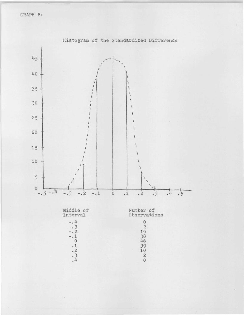
The histogram of the percentage appears to be bell shaped

with the limits being ±.3 (see Graph B). To determine if the

distribution is t-distributed with J4-• = 0 a t-test comparison is

performed after eliminating the outliers. The T value is 1.200.

The test is significant at .2323 which is within a 95% confidence

interval. A t-interval shows that 95% confidence interval is

located between -.0067 and .0071. The expected percentage

error for any given shipment is less than 17%.

The three outliers appear to be a major problem with the

predictive model. The outliers all have a common attribute

that no other shipment possesses. This attribute is that the

customer was charged for a service not included in the linear

model. The service was Transportation Section 9, which is a

storage in transit charge not a "moving" charge. These shipments

should be eliminated from the random sample because the linear

model is not supposed to predict their costs.

Discussion of the Acceptance Criteria

The linear model predicts the actual cost of the move.

A t value of -.299 for a t-test implies that the difference

between the actual cost and predicted cost is due to random

15

fluctuations and not due to inaccuracies. A test of significance

of .7655 implies that 75% of the time any other approximation

would be more inaccurate than this model. This model is more

than an accurate approximation; it is designed to be a predictive

model. The model's accuracy against uncontaminated data adds

credibility to the hypothesis that the linear model is actually

a predictive model.

The raw difference or the difference between the predictive

values and the actual values form a t-distribution with \ = 0.

The advantage of having \ = 0 is that neither the carrier nor

the national account gain or lose revenue from the aggrate of

shipments by using the linear model. Since the difference is

a t-distribution with ±800 as its limits, the range of the

gain or loss is limited and the probability of a large gain

or loss on an individual shipment is minimized.

The standardized values form a t-distribution with -H. = 0 .

The standardized value limits are ±.3 with a 95% confidence

interval of +.07. This demonstrates that the percentage gained

or lost is reasonable with respect to small weight shipments.

Under the old system the average amount of time spent

on rating an individual shipment is 20 minutes for calculation

of the line haul charge, and forty-five minutes for the calcu­

lation of the accessorial charges. These approximations are

supplied by Dow Tillman of Graebel Van Lines. Under the linear

model the amount of time spent on an individual shipment is 20

minutes for the calculation of the line haul charge and

16

approximately five minutes for determining the accessorial

charges. (For a better estimate of the time spent estimating

the accessorial charges see Appendix B.) The linear model has

more than halved the rating time from 65 minutes to 25 minutes.

Therefore, the linear model possesses ease of application.

The linear model possesses pricing adaptability in diverse

situations because criteria One (approximates the current tariff

system) was met in a sample of many national accounts. There­

fore, the model should be an accurate pricing model for any

national account. However, four adverse selection problems must

be discussed.

If the linear model is estimated across many national

accounts and used to price just a few national accounts, a

major problem could arise. The frequencies could be inaccurate

for one national account because consumer preference and the

internal variance may be self-correcting in a large sample. If

this self-correction exists, it would make the linear model

an accurate predictor for a sample of many national accounts

but an inaccurate predictor when applied to a few national

accounts. The linear model was constructed with the assumption

that the internal variance of the frequencies and consumer

preference are independent of their association with a specific

national account. There has yet to be discovered any evidence

that the assumption is invalid. However, the linear model

should never be used commercially for a national account until

its validity is checked against a random sample of that specific

national account's shipments.

17

The second problem, Akerlof adverse selection occurring

with rural and urban consumers, can probably be prevented (by

the model). Because of scheduling, there exists multiple prices

according to the customer's location. If these multiple prices

predict rural prices for the rural consumer and urban prices

for the urban customer, then there exist no incentives for

adverse selection. Since the linear model accurately predicts

the costs of moving a large sample which is a mixture of rural

prices and urban prices, the model might accurately approximate

the different prices experienced by differing consumers. This

should be explored more rigorously using aggregate testing with

a much larger random sample.

A form of adverse selection that the pricing flexibility

cannot eliminate is adverse accessorial selection. The linear

model charges the shipper the expected cost of an accessorial.

Shippers with few accessorials will not select the linear model

because they are being over-charged in comparison to the actual

costs of the move, while shippers with many accessorials will

transfer all of their business to the linear model price.

Although a shipper may know how many accessorials he

has, neither the national account nor the carrier have this

information available to them. Since the national account

decides which moves go to which van line, adverse accessorial

selection is prevented because the use of the model is only

legal at the national account level.

The final problem is adverse selection due to weight.

The linear model, being a line approximation, appears to have

18

an inherent flaw in its construction. The model underestimates

the charges of large weight shipments and overestimates the

charges of small weight shipments. The model was expected

to yield opposite results because of increasing or constant

returns to scale.

There are three possibilities that could explain this

problem. The first is that the actual cost versus weight could

be an S curve function. The second is that the violation of

assumption (the error terms are statistically independent)

might yield this result. The last possibility (I feel) is

the most likely. Many of the approximations were calculated

assuming the p's and m* s (see Appendix A) were fixed for all

weight classes. If either p or m were to minutely vary propor­

tionately with the weight, then this bias should be expected.

If the problem is caused by either the first or the third

possibility then the model may be refined as desired, but would

still remain a close approximation. If the problem is caused

by the violation of the assumption that the error terms are

statistically independent then the model is suspect. Further

work exploring these possibilities should be conducted.

The tariff structure (cash inflow) is determined by the

same standardized system and can be applied across all van

lines. However, the forms of revenue distribution (cash out­

flow) vary from van line to van line. One alogorithmic revenue

distribution method cannot be hypostulated. Therefore, the

discussion will be in the form of a generalization that needs

modification.

19

Revenue distribution is comprised of two parts: distribu­

tion of the line haul charge and distribution of the accessorial

charges. Since the line haul charge portion of the tariff

structure was not approximated, the method of distributing this

should not be changed. The purpose of accessorial revenue

distribution is to compensate agents for the accessorial services

they render. The hypostulated revenue distribution method

will attempt to adjust for the linear .approximation.

The accessorial revenue distribution model will be derived

in a similar manner to the linear model (see Appendix A). The

f• *r.• not only represents the expected cost to the shipper,

but f. *r.. also is the expected revenue of the carrier. The

f• *r. . should be rearranged into a series of estimators of

the total revenue. Since there exist five agents that receive

accessorial revenue distribution (Hauling Agent, Origin Service

Agent, Destination Service Agent, Packing Agent, and Unpacking

Agent), the new estimators will be HR, OR, DR, PR, UR, respec­

tively. Where R stands for revenue and IR =._.y,. such that

y. . is also revenue distribution compensation for accessorial i.

The agent who receives revenue distribution compensation is

responsible to see that the services (f.*r. •) are performed

for all i.

This system works as long as two different agents do

not perform one accessorial service. An example of this overlap

is packing. A packing agent (when he is not the hauler) will

leave a little bit for the hauling agent to pack. If the pack­

ing agent receives all of the packing revenue, the hauler is

20

not being fairly compensated for services rendered.

The accessorial revenue distribution model is easily modi­

fied to correct for this compensation flaw. A van line should

set an arbitrary percentage q of a service that the agent must

perform. If the packing agent must perform q percentage of the

packing, then the packing agent receives q times the packing

revenue and the hauler receives the rest. An illustrative

example:

If q = .97 and 1-q = .03, then

the hauler receives .03[a + b(cwt)], and

the packer receives .97[a + b(cwt)] where

a + b(cwt) = the estimator PR

Any other accessorial that displays overlap should be handled

in a similar fashion.

The problem with the accessorial revenue distribution

model is that the agent receives payment unconditionally.

Therefore, there exist incentives to circumvent the service

rather than to perform it. Since many accessorials (stair

carry, piano, waiting time, etc.) cannot be circumvented, the

problem only occurs in those accessorials that can be circum­

vented. The accessorials that can be circumvented must be

determined individually by case study for each different van

line. For those accessorials that can be circumvented, a system

must be determined that makes it economically unviable to the

agent to avoid rendering service.

The system proposed next has three attributes: economic

disincentives, economic incentives, and policing policy.

21

Penalties should be levied against agents who are derelict

in their performance of a service. The penalties should be

of a magnitude large enough to make it economically disadvanta­

geous to flirt with the system.

A van line is too centralized and removed to check that

all services are performed. Instead, the van line will rely

on agents to cross-check one another. If a penalty is levied,

a percentage should go to the agent who reported the discrep­

ancy. The agents will not protect fellow agents because it

is in the agent's best economic interest to ferret out and

report discrepancies. With agents cross-checking each other,

the probability of cheating going undetected for any length

of time is miniscule.

Some agents, who do not cheat the system, should be re­

warded for their perseverance. The remaining amount of money

from penalties collected should be redistributed among them.

This method of revenue distribution, although lacking direct

application, demonstrates that the linear model is condusive

to an acceptable revenue distribution program.

Summary

This paper established the need for a revised tariff,

derived a generalized linear model to satisfy the need, and

ran data through the generalized model to determine a specific

model. This specific model was compared against a set of four

criteria to determine if it was a viable alternative commercial

pricing mechanism. The model approximates the current tariff

22

(criterion One), possesses ease of application (criterion Two),

and assures an equitable form of revenue distribution (criterion

Four). However, the model may or may not prevent adverse selec­

tion (criterion Three). Two questions were left unresolved:

does the model prevent Akerlof adverse selection? and, can the

systematic bias be accounted for? Preliminary results presented

in this paper offer a tentative confirmation of these two ques­

tions. However, to establish the validity of the preliminary

affirmative findings, aggragate testing should be conducted

on a large sample and tests should be run to determine the

causes of the systematic bias. If the follow-up studies support

the preliminary findings, then the linear model is, without a

doubt, a commercially viable pricing mechanism. If the results

are negative, then the linear model needs some revisions before

it will be an acceptable alternative. No matter what the find­

ings of the follow up studies, the linear model will be either

a viable alternative pricing scheme or the theoretical break­

through that evolves into a new model which will become the

revised tariff.

Appendix A

The mathematical derivation of the linear model,

(a.. + b..(w) approximating Y..) will be explained in detail.

An accessorial charge is equal to the number of service units

performed, multiplied by the cost per unit. Therefore,

Y. . o r. .*f. iD ID i

Where: r. . = rate for accessorial i performed in county j

f. = number of service units perfo rmed.

The expected value of Y.. = Y.. implying that

$.. = E (r±j*f±).

The r. .'s are fixed by ICC regulations, therefore,

Y. . = r. .*E(f•) . ID ID i

Three different methods of determining E(f.) were employed.

The first was to assume f. occurred randomly with regard to

weight. The second was to assume f. varies linearly with weight.

The third was to assume that for a given weight class, (1000-

2500 lbs.) f- occurs randomly, but that the E(f-) of the

weight classes vary linearly with weight.

In the first method, the assumption states that the f.

occurs randomly; therefore, E(f.) can be expressed as a prob­

ability times the expected realization or number of occurrences.

B(f±) = P i* m i

where; p. = probability of accessorial i occurring

and: m. = expected number of occurrences when accessor­

ial i is realized. „

24

The calculation of p. and m. are derived as follows:

p. = s./n where s- is the number of shipments that acces­

sorial i occurred in and n is the total number of shipments.

m. = Q./s. where Q. = —• q.„ such that q-„ = the number 1 1 l l k£s. ^iK ^iK

of occurrences in shipment K.

Therefore, by substitution: E(f.) = Q-/n

In the second method, a linear regression was used to

estimate the expected frequency. Using Minitab II to run the

linear regressions on the actual f. frequencies yielded the

predictive model. This model was verified by inspecting the

2 • 2

R value, T ratio coefficient and F values.

The third method employs a combination of the two ap­

proaches just discussed. Because the accessorial occurs randomly

within a small given weight class (i.e., 1000-1250 lbs.), the

frequency of the accessorial within the weight class was deter­

mined by method one. The assumption made was that the expected

value of the weight class varies linearly with weight, even

though the frequency distribution of the accessorial does not.

The same type of linear regression model used by method two

was run on the expected frequencies for each weight class.

The linear regression was validated in the same manner as before.

In calculating the f-'s, two implicit assumptions were

made. The first was that the f^'s were statistically independent,

The second was that the f.'s were uniform for all counties.

A.3: Cov(f±*f .) = 0 for all i#j . ; A.4: E(f ) = E(fh) for all

g and h.

25

Because there exists so many counties in the U. S., to

simplify the tariff even further, every county j will be given

a designation v. v will aggregate counties with similar charac­

teristics together. Since there exists no method to determine

which counties had similar characteristics, a surrogate measure

was used. EAch county j is given a designation A thru L for

packing by the ICC. Presumably the ICC gives counties with

similar costs of productions the same designation; therefore,

the designations used by the ICC are the ones used by the linear

model.

Now every r.. will be replaced by r. . r. is the weighted

« ^

r. =z_ V- r. . where V • is the proportion of shipments in

average of the r.. _. ' s for all counties j with designation v.

y \

county j. Substituting: y.. = r. *f. which implies ̂ .. = r. J J ^ J1~J I V 1 „ r J11 IV

Q./n . The m u l t i p l i c a t i o n of r . by [Q. /n]Aexpress ion a, + X v IV J 1 ^ XV

b. (w) where a.. + b. (w) is the linear appropriation. IV IV IV ctr tr

The Y.. will be divided into four groups: origin service,

destination service, packing, and unpacking. Because the calcu­

lations for the four groups are identical, only origin service

(0.) will be demonstrated. The rest of the calculations can

be determined in a parallel manner. Define o. . = y. . if n *xi

and

only if y is an origin service accessorial. Since y.. = a.. •* xj i j

+ b..(w) + e. o.. = a. + b. (w) + e, by the previous condition.

Total origin service charge is equal to the summation of the JX>

individual origin service charges: 0. = -A-, o. .. Therefore,

0. = <d_(a. + b. (w) + e. ) which implies that 0. = A + B (w) + E

where Av = J ^ a ^ , B v = £Tibi v

a n d E = fr1e±. The expected

26

origin cost is a linear approximating ie, E(0.) - A + B (w)

because A and B are constants and E(E) = 0. v v

Since the y. .'s are grouped along two dimensions (the ith

dimension, or origin service, destination service, packing,

and unpacking,* and the jth dimension A thru L), a 4 x 12 matric

of costs is generated (see Table 1, Appendix B).

*Unpacking is scheduled 1-5 not A-L. Because unpacking is scheduled 1-5 by the ICC, this old schedule was maintained. Any attempt to rearrange it to fit the A-L designation unnec-cessarily increased the variance of the linear model. The unpacking and packing designations are adjacent, therefore there is not an increase in time or effort.

Appendix B

Table I

Destination Schedule Origin Service Service Packing Unpacking

Fee Cwt Fee Cwt Fee Cwt Fee Cwt

A 40.80 + .17934 (w) 25.93 + .15117(w) 138.30 + 7.4938(w)

B 40.90 + .31071(w) 25.93 + .17530(w) 145.30 + 7.7311(w)

C 41.51 + .33880(w) 26.05 + .19715(w) 148.79 + 7.9986(w)

D 42.15 + .47566(w) 26.25 + .22856(w) 152.78 + 8.2299(w)

E 42.10 + .48589(w) 26.21 + .30901(w) 158.05 + 8.5638(w)

F 42.06 + .49125(w) 26.12 + .34985(w) 163.92 + 8.8759(w)

G 44.62 + ,53755(w) 26.75 + .33046(w) 168.86 + 9.1725(w)

^ H 46.94 + .58655(w) 27.78 + .35728(w) 176.10 + 9.5896(w)

I 47.30 + .51714(w) 28.20 + .38934(w) 181.76 + 9.9634(w)

J 49.40 + .65693(w) 29.88 + -41750(w) 190.86 +10.4391(w)

K 49.05 + .69010(w) 28.43 + .44204(w) 198.85 +10.4312(w)

L 50.68 + .76540(w) 29.17 + .50542(w) 207.34 +11.4332(w)

1

2

3

4

5

24.33 + 1.2458(w)

26.86 + 1.4837(w)

28.25 + 1.5585(w)

31.22 + 1.7347(w)

34.92 + 1.9485(w)

Appendix B

Table II

County Type Charge

Origin Service 1 2

Destination Service 3 4

Packing Service 5 6

Unpacking Service 7 8

Line Haul Charge 9

Sub Total 10

Total Cost 11

Step One: Enter ICC packing destination for the origin county in blanks 1 and 5.

Step Two: Enter the ICC packing designation for the destina­tion county in blank 3.

Step Three: Enter the ICC unpacking designation for the destina­tion county in blank 7.

Step Four: If either packing or unpacking service is not performed, enter zero in the charge column blanks 6 and/or $

Step Five: Determine the appropriate charge from Table I, enter it in blanks 2, 4, 6, 8. (Example: Destina­tion 0 County type "D", the charge for destination service is 26.25 + .22856(cwt)). This number would be entered in blank 4.

Step Six: Enter the line haul charge rate in blank 9.

Step Seven: Add the charges together. (Add blanks 2, 4, 6, 8, 9 Enter in line 10.

Step Eight: In line 10 substitute the cwt of the shipment for w. Do the necessary algebra to simplify to a single number. Enter this number in blank 11. This is the total charge of the shipment.

28

Footnotes

John Hess, The Mobile Society: A History of the Moving Industry (New York, New York: McGraw-Hill, 1973), p. 63.

2Ibid., p. 14 9

3Ibid.

4Ibid., p. lit

5Ibid., p. 119

29

Bibliography

Akerlof, George A. "The Market for "Lemons' Quality Uncertainty and the Market Mechanism*" The Quarterly Journal of Economics, No. 33, August 1970.

Allied Van Lines Regulation Manual. . . . * .

Bekin Van Lines Flat Rate Tariff? REgulation Manual? Tariff 412.

Bunsendahl? Jr«p Sidney P. "Evaluation of Household Good Carrier" s Servic©18 by the Department of Defenser 1980«,

Coxr John R» "Moving Cost Estimating % The Ongoing Controversy."

Csoiego, M. Stro^ Approximations in Probability and Statistics. New Yorks Academic Pressg 1981.

=

Graebel Van Lines Bill of Ladings? Regulation Manual; Tariff 400? Tariff 104.

Bess, John„ The Mobile Societys A History of the Moving Industry7, New Yorks McGraw-Hill^"iffTjI

Household Goods Transportation Act 198® <,

Jessen, Raymond James. Statistical Survey Techniques. New Yorks Wileyt 1978.

Korin, Basil Po Statistical Concepts for the Social Services. CambridgeB Masss Winthrop7 1975.

Motor Carriers Act of 1979 <=

Phillips, Lawrence Do Bayesian Statistics for the Social Scientists. London% Nelson, 1973.

1/1 ]/jtL ft 6lU^

30