A project of Volunteers in Asia

A Sitinu Handbook for Small Wind Mneruv Conversion Svstems

by: Harry L. Wegley, Montie M. Orgill and Ron L. Drake

Published by: United States Department of Energy Washington, DC USA

Paper copies are $ 9.00; quote accession number PNL 2521 when ordering.

Available from: National Technical Information Service U.S. Department of Commerce Springfield, VA 22161 USA

Reproduction of this microfiche document in any form is subject to the same restrictions as those of the original document.

PNL-2521

A SITING HANDBOOK FOR SMALL WIND ENERGY CONVERSION SYSTEMS

HARRY L, WEGLEY, ET AL

BATTELLE PACIFIC NORTHWEST LABORATORIES ZICHLAND, WASHINGTON

MAY 1978

Pacific Northwest laboratory Richland, Washington 99352 Operated for the U.S. Department of Energy

bY

QEPR00UCE0 BV

.

9

.

.

PNL-2521 UC-60

A SITING HANDBOOK FOR SMALL WIND ENERGY CONVERSION SYSTEMS

by !Iarry L. Weqley Montie M. Orgill Ron L. Drake

DAI'TELLE Pacific Northwest Laboratories Richland, Washington 99352

\

Prepared for the U.S. Department of Energy, formerly the Energy Rsearch and Development Administration, under Contract EY-76-C-06-183C.

I-

The primary purpose of this handbook is to provide Siting

guidelines for laymen who are considering the use of small *-ind energy conversion systems. With this purpo e in mind, the handbook is being published in its current form to p e basic strategies to users as early as possible. The handboo son require updating due to rapidly changing technology and the evolving needs af users. Consequently, the authors also intend for this edition to serve as a review copy prior to wider dis

The authors wish to thank Dr. m Pennell for the techni- cal guidance he provided, Dr. Carl Aspliden and Dr. Craig Hansen for their review@ Jeanne McPherson and Chris Gilchrist for their help in editinq, and Rosemary Ellis for her helpful suggestions and the many hours of typing she contributed. The writing of this handbook and the associated research were sponsored by the Depart- ment of Energy, Wind Systems ranch.

iii

CONTENTS

F:;FI:.gk:ORD . 0 . . . . . .

1.0 IkiTRODUCTION , . . . . *

TASK A-- Preliminary Feasibility Study .

TASK B--Site and System Selection . .

2.3 :;mERAL Dk:SCRlPTION OF THE WIND . .

2.1 GENERATION OF THE WIND . . .

2.2 INFLUENCES ON AIRFLOW . . . -I -1 L.2 EFFECTS OF SURFACE ROUGHNESS . .

2.4 AVAILABLE POWER IN THE WIND . .

3.0 ENVIRONMENTAL HAZARDS TO WECS OPERATIONS 3.1

3.2

3.3

3.4

7 E 4.d

3.6

3.7

3.8

3 * 9

TURBULENCE . . . STRONG WIND SHEAR . . EXTREME WINDS . . .

THUNDERSTORMS . . . ICING . 0 .

HEAVY SNOW . . . FLOODS AND SLIDES . . EXTREME TEMPERATURES . SA!~?' SI-RAY AND BLOWING DUST

‘4 . 0 51 ‘I’ING 1 N F’i ~411’ TERRATN . .

4.i UNZFOIIM !?OUGiINLSS . .

4.2 CHANGES IN ROIJGHNESS .

4.3 BARRIERS IN FLAT TERRAIN 4.3.1 Buildings m . 4.3.2 Shelterbelts .

4.3.3 Individual Trees .

4 . 3 e 4 :-:catt.ered Barriers :I Ai: " 1 Id\, IN ivt)F\j-F;,t"\'l' ‘i’F:RF&IN .

‘. I ;? ll)~;l;‘~ . . . .

‘1 . L! ! :I\ ( ~:I,~,'l'::it II I l_:i,:; r\NU MOUNTAINS !, 3 I * ,; :; y , ' I I. /',>I'3 si!D[JI,F::; * . 'I . 4 <:r’il‘i; ;\Ni) r;OJti;l,:S . .

.

.

.

.

.

.

.

.

.

.

.

.

.

.

.

.

.

.

.

.

.

.

.

.

.

.

.

.

.

.

.

.

.

.

.

.

.

.

a

.

.

.

.

.

.

.

e

.

.

.

.

.

.

.

.

.

.

.

.

.

.

.

.

.

.

.

.

.

.

.

.

.

.

0

*

.

.

.

.

.

.

.

.

e

.

.

.

.

.

.

.

.

.

.

.

.

.

.

.

.

.

.

.

.

.

l

.

.

. iii . 1.1 . 1.2 . 1.3

. 2.1

. 2.1

. 2.1

. 2.1

. 2.2

. 3.1

. 3.1 e 3.2 . 3.3 . 3.3 . 3.7 . 3.10

. 3.10 . 3.10 . 3.12 . 4 . 1 . 4.2 . 4.7 . 4.11 . 4.11

. 4.15

. 4.20

. 4.21 . 5. 1 a 5.1 * 5.9 . 5.11 . 5.12

V

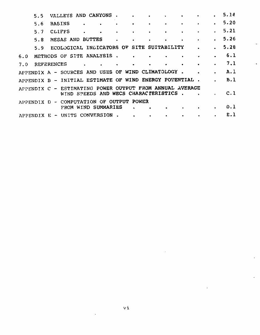
5.5 VALLEYS AND CANYONS . . . e . . 5.6 BASINS . . t . . . . . 5.7 CLIFFS . . . . . . . . 5.8 MESAS AND BUTTES . . . . . . 5.9 ECOLdGICAL INLICATORS OF" SI SUIT ITY .

6.0 METHODS OF SITE ANALYSIS . . . . . . 7.0 REFERENCES . . . . . . . . APPENDIX A - SOURCES AND USES OF WIND CL TOLOGY . . APPENDIX B - INITIAL EST1

APPENDIX C - ESTIMATING P WIND SPEEDS AND WECS

APPENDIX D - COMPUTATION OF OUTPUT PO FROM WIND SUMMARIES . . . . .

APPENDIX E - UNITS CONVERSION . . . . . .

.

.

.

.

.

.

5.14 5.20 5.21 5.26

- 5.28 6.1 7.1 - A.1 B.l

C.l

0.1 E.1

Vi

LIST OF FIGURES

2.1 Effect of Surface Friction on Low-Level Wind . .

2.2 Definition of the Rotor Disc . . . . . 3.1 Simple Method of Detecting Turbulence . . .

3.2 The blaximum Expected Winds for a 5O-yr Me2n Recurrence Interval . o . .

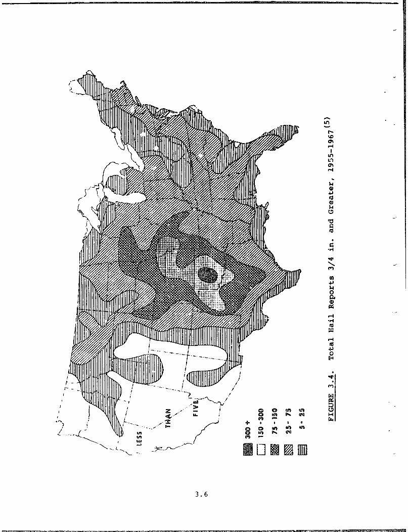
3.3 The Mean AnIlual Number of Days with Thunderstorms . !.4 '12-3ti~ 1 fi,~ 1 I Rl~~~1rt.6 J,'4 in. and Greater, 1955-1967 . 3.5 'l'ornado Strikcl Probability Within S-Degree Squares

. in the Continental Clnited States . . 3.6 Number of Times Ice 0.25 in. or More Thick

Was Ubservcd During the 9-yr Period of the Association of American Railroads Study .

3.7 Extreme Storm Maximum Snow Fall . . 3.8 Annual Percent Frequency of Dusty Hours .

4.1 Determination of Flat Terrain . . . 4.2 Formation of a New Wind Profile

Above Cround Level . . . . . 4.3 Wind Speed Profiles Near a Change in Terrain 4 * 4 Tratlsition Height in Wind Speed Profile

IJut: to a Chanqc RoucJhncss . . . 4.5 ~XdilllIlC C>f Ci '!‘ransition Height Diagram

Depictlllij (jnc: Challgc in Roughness . . 4.6 ,\i ~-flow Rrot;rld rl Block Building . . ,i .7 Zone: of Disturbecl Flow over a Small Building 4.8 I'ht: Effects of a11 undisturbed Airflow

Encountering an Obstruction . . .

.

.

.

4.9 Airflow Near a. Shelterbelt . . . 4.10 Percent Wind Speed at Different Levels Above

the Surface Behind a Row of Trees of Height, 4. il The Zone :~f 'r,urbulence Behind a Shelterbelt :J . 1 !;ciinit ioll or a Ridilt2 . . . .

H

.

.

.

.

.

.

.

.

.

.

.

.

.

.

.

.

.

.

.

.

.

.

.

.

.

.

.

.

.

.

.

.

.

.

.

.

.

.

.

.

.

.

.

1

.

.

2.3

2.4 3.2

3.4 3.5 3.6

3.8

3.9 3.11 3.13

4.2

4.7 4.8

4.9

4.10 4.12 4.13

4.13 4.16

4.17 4.18

5.2 5.3

5.4

5.5

vii

5.5 Percentage Variation on Wind Speed over an Idealized Ridge . . . . .

5.6 Hazardous Wind Shear over a Flat-Topped Ridge 5.7 Effect of Surface Roughness on Wind Flow

over a Low Sharp-Crested Ridge . . . 5.8 Airflow Around an Isolated Hill (Top View) . 5.9 A Schematic of the Wind Pattern and Velocity

Profile Through a Mountain Pass . . . 5.10 A Schematic Illustrat-ion or' Flow Patterns that

May Be Observed Through Gaps and Gorges . . 5.11 The Daily Sequence of Mountain and Valley Wir?ds 5.12

5.13

5.14

5.15

5.16

5.17

5.18

5.19

5.20

5.21

A.1 A.2

A.3 B.l 1%. ,‘

l1‘. 1

c.-. 2

c . 3

D. 1

Vertical Profile of the Mountain Wind . . Possible WECS Sites in Sloping Valleys and Canyons . . . . . . . Possible WECS Sites Where Prevailing Winds are Channeled by Valleys . . . . . Airflow over Cliffs Having Differently-Slcped Faces . . . . . Top View of Airflow over Concave and Convex Portions of a Cliff Face . . . . . Vertical Profiles of Air Flowing over a Cliff The Effects of Upwind Roughness on the Location of the Best WECS Site Downwind from a Cliff . Flow Around and over Buttes and Mesas . . Wind Speed Rating Scale Based on the Shape of the Crown and Degree Twigs, Branches, and Trunk are Bent (Griggs-Putnam Index) . . . Deformation Ratio Computed as a Measure Of the Degree of Flaqcli.ng . . , - l

Sample Wind Rose . . . . l l

Nuclear Power Plant Sites . . l l

Sample Wind Energy Rose . . . . l

Available Wind Power--Annual Average . l

Annull-Averaqe Wind Power at tliqht>r l<lk\v;~tions, in Watts/m 3

0 m Above . . .

1:stimatc of Exi)cctt-d Average Power Output for Wind Turbinc,s . . . . . . Percent Down Time . . . . . .

PiFrcent- Time Running at Rated . . . . Hypothct:1c;lI Output Power Curve . . .

viii

.

.

.

.

.

.

.

.

.

.

.

.

.

.

.

.

.

.

.

.

.

.

.

.

.

.

.

.

.

.

.

.

.

.

.

l

.

.

.

.

.

.

.

.

.

.

.

.

.

.

.

.

5.6

5.7

5.8 5.10

5.13

5.14 5.16 5.17

5.18 r7

5.19

5.22 .I 5.23 5.24

5.25 5.27

5.29

5.30 A.3 A.4 A.5 B.2

B.3

c.2 c.3 c.3 D.3

i,LST QF TABLES --_-- -

2.1 Ferccntage Change in Available Power with Changes in Wind Speed . a . .

4.1

4.2 4 7 .J 4.4

Extrapolation of the Wind Speed from 30 ft to Other Heights Over Flat Terrain of Uniform Roughness . . . l . . .

Power Change Due to Extrapolation to a New Height Wake Behavior of Variously Shaped Buildings . Available Power Loss and Turbulence Increase Downwind from Shelterbelts of Various Porosities

4.5 5.1

5.2 5.3

5.4

Speed and Power Loss in Tree Wakes . . WECS Site Suitability Based Upon Slope of the Ridge . . . . . WECS Site Suitability on Isolated Hills . Mean Annual Wind Speed Versus the Griggs-Puttnam Index . . . . Mean Annual Wind Speed Versus the Deformation Ratio . . . . .

5.5 Griggs-Putnam Index Versus Annual Average Wind Speed for Conifers in the Northeastern United States . . . . . .

6.1 Various Approaches to Site Analysis . A.1 Sample Wind Summary . . . . . 0.1 New Wind Summary . . . . . D.2 Hypothetical Wind Summary . . . D.3 Xypothetical Output Power by Speed Class 1). 4 Conversion of 8 Frequencies to Hours u

.

.

.

.

.

.

.

.

.

.

.

.

.

.

.

.

.

.

.

.

.

.

.

.

.

.

.

.

.

. 2.5

. 4.4

. 4.6

. 4.14

. 4.19

. 4.20

. 5.6

. 5.10

. 5.31

. 5.31

. 5.32

. 6.2

. A.2

. D.l

. D.4

. D.4

. D.4

ix

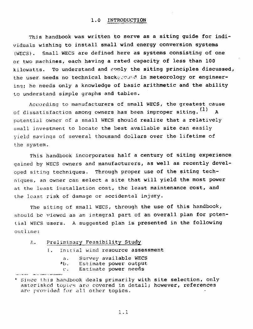
1.0 INTRODUCTION

This handbook was written to serve as a siting guide for indi-

viduals wishing to install small wind energy conversion sys’tems

(WECS). Small WECS are defined here as systems consisting of one

or two machines, each having a rated capacity of less than 100

kilowatts. To understand and c~nly the siting principles discussed,

the user.needs no technical backi ,-o~l*r;\?. in meteorology or engineer-

inq; he needs only a knowledge of basic arithmetic and the ability to understand simple graphs and tables.

According to manufacturers of small WECS, the greatest cause of dissatisfaction among owners has been improper siting. (1) A

potential owner of a small WECS should realize that a relatively small investment to locate the best available site can easily yield savings of several thousand dollars over the lifetime of the system.

This handbook incorporates half a century of siting experience gained by WECS owners and manufacturers, as well as recently devel-

oped siting techniques. Through proper use of the siting tech-

niques, an owner can select a site that will yield the most power at the least installation cost, the least maintenance cost, and the least risk of damage or accidental injury.

The siting of small WECS, through the use of this handbook,

should bc viewed as an integral part of an Overall tial WECS users. A suggested plan is presented in outline:

plan for poten- the following

E: . Preliminary Feasibility Study I A. In;cial wind resource assessment

a . Survey available WECS *I.),. Estimate power output c‘. Estimate power needs

----- I -- _---- * Sillce this handbook deals primarily with site selection, only

asterisked topic-s arc? covered in detail; however, references ark‘ pt-ov ided for 21.1 other topics.

3

2. Economic analysis

E: Analyze cost of WECS Consider legal (and other) factors

C. Formulate working budget

B. Site and System Selection 1. Final wind resource assessment

*a. Select candidate site *b. Determine availab.le power at candidate site

2. Selection of WECS a. Estimate power needs quantitatively

"b. Estimate power output quantitatively C. Choose WECS and storage/backup system

3

The following step-by-step procedure is suggested as a method of integrating the siting handbook and other references to accom-, plish the tasks in the planning outline:

TASK A--Preliminary Feasibility Study

To make the initial wind resource assessment, take the follow- ing steps:

1. Obtain information on costs and operating characteristics of available WECS. The American Wind Energy Association can provide lists of manufacturers and distributors from whom this information can be obtained. The address is:

American Wind Energy Association 54468 CR 31 Bristol, IN 46507

2. Use the information in Appendix B of this handbook to make a rough estimate of wind power potential. If there is lit- tle potential, wind energy will probably not be competitive with other energy sources.

-a J. r’3’7S~:~t <? ‘-,-opy of p;jr,d power for L ., L . Farms, Home, and Small B-usi- ncsses by J. P,lrk and D. Schwind, -- available on written request (see r~efcrellct~ 2) . This booklet contains much practical infor- mation which complcmccts the siting handbook.

4

J

1.2

1. Roughly estimate eneryy needs (both average load and peak

load). Consult a WECS dealer and/or Chapter 4 of Refer-

ellCt? 2 for dssistnrce.

5. Llsing Appendix C of this handbook, estimate power output for several available WECS. Will any of them produce suf-

ficient power? If not, can energy conservation make up the

energy deficit?

o analyze the economics of the WECS, take the following steps:

1. If a WECS appears to meet power requirements, compare esti- mated WECS costs (over the life expectancy of the WECS) to the projected costs of conventional power for the same period. Chapter 6 of Reference 2 gives instructions for a thorough economic analysis.

2. Consider the impact of all economic restraints, such as available funds, legal, environmental, and other concerns (see Chapter 7 of Reference 2).

3. Formulate a working budget from this information if wind energy appears feasible.

'ASK B--Site and System Selection

To m;Ilke the final wind resource assessment, take the follow- ng steps:

1. Read Sections 2 and 3 of the siting handbook for essential information on the nature of wind, wind power, and WECS hazards.

3 L. Read the introduction to Section 4; classify terrain as flat

or non-flat.

.? . Tf Terrain is non-flat: .-- - ----- -- (1) Read %?C:tiCJIlS 4.1 and 4.2 for background. (2) Ticad the l>ortions of Sections 4.3 and 5 that

!I(‘,1 1 ~iih lizrricrs or terrain features in or llr',lr t hc :;itincl area.

1.3

(3) Follow siting guidelines given to select the best candidate site(s).

b. If terrain is flat: (1) Read Sections 4.1 and 4.2 for background. (2) If the surface roughness(a) is uniform, select

candidate sites by reading applicable portions of Section 4.3.

(3) If there are changes in roughnessB consider those effects in conjunction with the applicable por- tions of Section 4.3 to select candidate site(s).

3. Read Section 6 of this handbook and select a method of site evaluation; begin data collection (or arrange to have it done).

To select a WECS, take the following steps:

1.

2.

3.

W!,en all site evaluation data have been collected, use guide- lines in Section 6 of this handbook to make final estimates of output power for.various WECS.

Make a detailed estimate of energy needs if this was not done in the feasibility study (a WECS dealer and/or Chapter 4 of Reference 2 can provide guidance).

Select the WECS that meets energy requirements at the lowest cost.

. - I - - -_ ___- __

(rf) Surface rou!7hness is explained in Section 2.3.

1.4

2.0 GENERAL DESCRIPTION OF THE WIND .-

2.1 GENERATION OF THE WIND

The ultimate energy source which drives the wind is the sun.

Incoming solar energy, which generally decreases from the equator

to the poles, is absorbed and reflected differently by various

parts of the atmosphere and by the various types of surfaces (i.e., oceans, snow, and ice, sandy deserts, forests, etc.). The redis-

tribution of incoming solai' energy tends to produce low and high

pressure areas.

Pressure differences in the atmosphere force the air to move toward lower pressure. Once the air begins to move, other factors

modify both its speed and direction.

2.2 INFLUENCES ON AIRFLOW

Pressure systems (frequently 500 to 1000 miles or more in diameter), which are associated with large-scale wind patterns, tend to migrate from west to east across North America. As the

air in the large-scale wind pattern moves through local areas, its speed and direction may be changed by the local topography and by local heating or cooling. At a particular WECS site,

trees, buildings or other small-scale influences may further dis- turb the wind flow. The combined effects of these three scales

of influence produce hiyhly variable winds.

2.3 EFFECTS OF SURFACE ROUGHNESS

The surface over which the wind flows affects wind speed near that surface. A rough surface (such as trees and buildings) will produce more friction than a smooth surface (such as a lake). The

qrcater the friction the n-:ore the wind speed is reduced near the surface.

2.1

Figure 2.1 illustrates how surface roughness, affects wind speed by means of a vertical wind speed profile--simply a picture of the change in wind speed with height. Within 10 ft of the sur- -

face, wind speec; ';.s greatly reduced by friction. Wind speed 4

increases, howevtir, between the surface and 1000 ft as the effects

of surface roughness are overcome. Knowing how

ness affects the vertical wind speed profile is when determining the most beneficial WECS tower

- the surface rough- extremely valuable height.

2.4 AVAILABLE POWER IN THE WIND

To find a site with the most available wind power, it is essential to have a clear understanding of the variation of power with wind speed. The following equation defines this relationship:

Available Power = 0.5 x D x A x S3

where

D = air density r\, : ;lrc!,s of the\ rotor disc S = the wind speed (S 3 = s x s x s, cube of wind speed).

Rotor discs (mentioned in the above equation) are illustrated in Figure 2.2 for three different types of WECS. Since air density (D) at a site normally varies only 10% or less during the year, the amount of power available depends primarily on the area (A) of the rotor disc and the wind speed (S). Increasing the diameter of the rotor disc (by increasing the blade length) will allow the WFCS to intercept more of the wind, and thereby harness more 1" '\Gl‘l‘ . ( a )

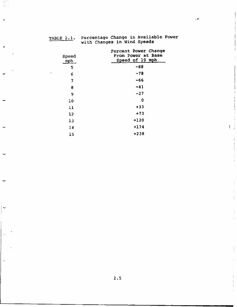
:: i ll('c- I 11t- ;lvlli7nblc power varies with the cube of the b' I IlkI S) wt‘ll , l'llcm:i I1111 ;1 site> where wind speed is greatest is desir- cl 11 1 t.' . T,ll) lc> 2 . 1 ~iemonstrates how even a small change in wind 5Iwcil results in .I larqe change in available power. Suppose that

- (*I! 'I'll, ) I*III 1 i (-1’ ;J t WKS size should not be made solely on this

It,15 i L:, I\111 i11 (~~niunction with the WECS dealer and/or Sec- I il)tl il 01 I II I !: I~‘lllci~lo<~k.

2.2

laa, FEET 2oMPH (SPEED UNAFFECTED BYSURFACE)

; I I 1 ~‘5MPl-l -I------------ i

10 FEET (SPEED REDUCED BY FRICTION WiTH SURFACE)

FIGURE 2.1. Effect of Surface Friction on Low-Level Wind

one computation of available power at a site had been based on a wind speed estimate of 10 mph when the actual speed was 9 mph. The actual available power would be almost 30% less than the esti- mated power due solely to a one mph error in the estimated wind speed.

To estimate the available power in the entire year it is necessary to estimate how frequently each wind speed occurs. The value that the user places on accurate estimations of available power will ultimately determine the time and money he is willing to spend to measure the annual frequencies of wind speeds at his site. Various approaches to wind data collection are discussed in Section 6.

tkfore a site is chosen, the user should know how available power and wind direction vary in the area, A convenient way of expressing this relationship is through the use of a wind energy rose , .I ql:aph i(.- representation of the amount of wind energy asso- c.i at-cd with each wind direction. If a potential WECS user has iivtiJ ;lt a loc,lt:ion for a long period of time, he may intuitively

2.3

(HORIZONTAL AXIS ROTOR)

FIGURE 2.2. Definition of the Rotor Disc -.

know the principal power direction (i.e., the win? direction which

will contain most of the available power).' kowev&, if data from

a nearby observing station are available, a wind energy rose should

be constructed from the sumarized data (see Appendix A for defi- -. nition, methods of construction, and use of'wind ekkgy roses).

2.4

,

TABLE 2.1.

c

Speed mph

5

6

7

8

9

10

11

12

13

14

15

Percentage Change in Available Power with Changes in Wind Speeds

Percent Power Change From Power at Base

Speed of 10 mph

-88

-78

-66

-41

-27

0

+33

+73

+120

at174

a238

2.5

3.0 ENVTRONMHN'I'AL tIAZARDS TO WECS OPERATIONS -__-- --

Fnvircnmental hazards may influence the economic feasibility

of a WECS or the selection of a particular machine. For example,

if salt spray at a coastal site reduces the expected lifetime of

a WECS by one-half, the cost of wind energy to the user sharply

increases. Good siting strategy, therefore, will not only maximize

the wind speed, but also reduce hazards.

Many WECS hazards cannot be avoided. In such cases, the user

must either purchase a WECS designed to survive in the local envi-

ronment or in some way protect the WECS from the hazard. The

potential economic impact of either approach must be evaluated.

3.1 TURBULENCE

Air turbulence consists of rapid changes in speed and/or

direction of the wind. The turbulence most harmful to WECS is the

small-scale, rapid fluctuation often caused by the wind flowing

over a rough surface or a barrier. Turbulence has two adverse

effects: 1) a decrease in harnessable power and 2) vibrations and

unequal loading on the WECS that may eventually weaken and damage

it.

To characterize the turbulence at a site, the user should

ttctermine the prevailing wind power direction (see Use of Wind

!;ummaries in Appendix A). (a) When the prevailing wind is blowing,

Ili~! \l1-cc1olilin,lnt arca:; of turbulence at a proposed WECS site can be tlc\tel-ted by 011~' or marc' 4-ft lenqths of ribbon tied to a long pole,

kite string, or strinq of a large helium-filled balloon. How much

the ribbons flap indicates the amount of turbulence. A second .-;trinq can lx used to pull a balloon or kite into position over t hl> k!F.:C:; , si,te isec' Fiyure 3.1) to determine the height to which

\ .1 ) 1 !’ mL>rc tlmn one KI rid direction frequently occurs, the user ~l~oulci invl?st. i.gatc each to understand the turbulence hazard

3.1

TOP OF BARRIER- . INDUCED TURBULENCE

FIGURE 3.1. Simple Method of Detecting Turbulence r

turbulence extends. The expected location and intensity of turbu-

lence produced by barriers and landforms are described (at least

qualitatively) in Sections 4 and 5.

3.2 STRONG WIND SHEAR

Strong wind shear may pose a hazard to small WECS in some

locations. Wind shear is simply a large change in speed or direc-

tion over a small distance. If a large change occurs over a dis-

tance less than or equal to the diameter of the rotor disc (see

Figure 2.2 for definition of rotor disc), then unequal forces will be acting on the blades. Over a period of time these forces could

damage the WECS.

Ccncrally the longer the blades, the more susceptible the Twl:c-r, is to shear hazards. However, shear can be a hazard to any a:: 'F. :,.,Jsc rotor disc is too near the ground, a canyon wall, a stct:p mollntain side, or the top of a flat-topped ridge, (see Fig- u “<, 5.! ).

3.2

3.3 EXTREME WINDS

WECS blades and the supporting towers are both susceptible

to damage from high winds. The blades become vulnerable if the

protection systems designed into many WECS fail in extreme winds.

Towers must be capable of supporting the WECS in all wind speeds

which normally occur in the local area.

Figure 3.2 shows maximum wind speeds which might occur in a

50-yr period. However, since this is a national map, some local

areas of very high winds (mostly in the Rocky Mountains). have been

omitted. Users in or near mountains should obtain extreme wind

speeds from nearby weather stations when planning a WECS (see

Appendix A for sources of wind data).

The WECS dealer may assist in selecting the best tower, but

before it is purchased, the user should contact local building

inspectors to insure compliance with existing codes.

3.4 THUNDERSTORMS

Thunderstorms produce several hazards, such as severe winds,

heavy rains, lightning, hail, and possibly tornadoes. Figure 3.3

shows that thunderstorms occur on over 40 days per year in most

parts of the United States. The largest number and most intense

tl-iiiri&erstorms occur in Florida and the Great Plains states of

Kansas and Oklahoma.

Though the frequency of lightning is not available, it can be

;)‘I:-tially inferr-ctd from the thunderstorm occurrences shown in

1.’ i ( I I 11-e 3 . 3 . C'clllr;idt:rinq its cost, a WECS should be protected from 1 tL;llt llini; st rl kc>)l; wht~r(:vc~r it is located.

iI;lii cjftcn causes tleavy damage to buildings: it may also

c,:lu:;e clan,acj;e to il wind machine and its support structure. Large h:1il is most frequently observed in Texas, Oklahoma, Kansas and NV !il~.lSL,‘I il'iqllri‘ 3. 4; .

3.3

\

.:

_L MAXIMUM EXPECTED WINDS !iO-YEAR MEAN RECURRENCE INTERVAL”

~acd on data thr&h 19t.S [.i ] .~~ -1

Adant from a M0,000,000-%ule map hy 0”

Entir~m&ml Data Service. Es% p@@e$ in AXE: %& p. 093 III 0 -._- -_ - __--- --.- -----

. . 1 -... ,,r)- II ..)

c

FIGURE 3.2. The Maximum Expected Winds for a SO-yr Mean Recurrence interval(3)

I

I I

1 I 1 I j I

I i

i

P

u

3.6

Tornadoes occur most often in the central part of the United

States in an area called "tornado alley," extending from south-

western Texas to northern Illinois. Figure 3.5 shows the

approximate risk of a tornado strike for different areas of the

continental United States. Since WECS, like houses, are not

designed to withstand tornadoes, the prospective buyer must assess

the risk of tornado damage.

3.5 ICING

rce accumulated on blades, towers, and transmission lines can

cause hazards or reduce the efficiency of wind machines. There

are two types of icing: rime ice and glaze ice.

Rime ice differs from glaze principally because of its source.

It forms from frost or freezing fog rather than rain. Rime icing

occurs mainly at high elevations. It is drier, less dense, and

therefore less hazardous than glaze: however, it can, over a period

of time, build up large accumulations.

Glaze icing, formed from freezing rainc occurs most frequently

in valleys, basins, and other low elevations. When rain falls

through a subfreezing layer of air at the ground, the drops freeze

on contact with the surface. Under favorable conditions, freezing

precipitation can rapidly accumulate on a cold surface to thick-

nesses c)f more than two inches. Data gathered by the Association

of Amcr Lean Railroads, Edison Electric Institute, American

Tc1cphor.c and Tclcql aph, and other orqanizations on ice accumula-

tion on transmission llncs in the United States have been analyzed

for the period 191L-1938; the number of times icing greater than

0.25 in. occurred is shown in Figure 3.6.

3.7

00 9-11

l-2 12-14

3-5 15-18

6-8 18t

FIGURE 3.6. Number of Times Ice 0.25 in. or More Thick Was Observed During the 9-yr Period of the Association of American Railroads Study(T)

3.6 HEAVY SNOW

Snow causes three principal hazards to a WECS: 1) service 4

and maintenance can be made difficult by excessive snow depths;

2) excessively heavy snowfall may damage parts of the turbine; and

3) blowing snow may infiltrate the machine parts and causle break-

age from freezing and thawing.

Figure 3.7, which shows the maximum snow depth for a storm

period, is provided as a guide for estimating snowfall. However,

iIl some mountain regions much more snowfall has been recorded than

is shown on the map. How long a typical storm lasts and how long

SIIC)W rcma ins oii the grcuzd arc also important considerations.

As the figure illustrates, the high wind areas on the eastern

sides of Lake Superior and Lake Michigan receive more snow (as

much as 60 in. or more per year) than the area beyond these snow-

belts. A potential user considering a site on the eastern sides

of the Great Lakes should therefore consider the damaging effects

of heavy snowfalls and blowing snow.

d

4'

&

3.7 FLOODS AND SLIDES --

Floods and slides arc locai problems which users of WECS will

bt- aware of. In cjcncra.l, all structures should be kept out of

f l.oodplains. If an ideal wind site is located in a river valley,

the user should build a structure to withstand flood conditions.

He should also investigate the potential for earth slides and the

stability of the soil foundation at any potential wind site. J

3.8 EXTREME TEMPERATURES --

Extremely high or low temperatures will adversely affect most

hxCS, Lubricants frequently freeze in very cold temperatures, - d , causing rapid wear on moving parts. Many paints, lubricants, and

3.10

FIGURE 3.7. Extreme Storm Maximum Snow Fall (81

other protective materials deteriorate in high temperatures.

user should review the local climatology and then consider the

possible added expense of protecting the WECS against extreme

temperatures.

3.9 SALT SPRAY AND BLOWING DUST

Salt spray and dust may damage a WECS unless the machines are

properly constructed and maintained. The corrosive properties of salt spray should be taken into account for any site within 10 miles

of the sea.

Blowing dust may damage the system if it penetrates the moving

parts, such as the gears and turning shafts. Many diverse regions ef +hn ~.-.a~n++-.- -.I- -,,A*L.l~ (urban,

- ---. cayjr lc=uit~urai, desert, vailey and plain areasj

are subject to suspended dust. However, mountainous, forested and coastal regions have few major dust storms. The highest frequency of dust occurs in the southern Great Plains, but blowing dust also

occurs often in portions of the western states, northern Great

Plains, southern Pacific Coast and the southeast (see Figure 3.8).

3.12

F'igure 3.8. Annual Percent Frequency of busty Hours. (Based on hourly observations from 343 weather observation stat'ons that recorded dust, blowing dust and sand when prevailing visibility was less than 7 mi (11 km). Shaded

areas (N) represent no observations of dust. Period of record is from 1940 to 1970.) (9)

4.0 SITING IN FLAT TERRAIN

Choosing a site in flat terrain is not as complicated as

choosing a site in hilly or mountainous areas. Only two primary

questions need be considered:

0 What surface roughnesses affect the wind profile In the

area?

e What barriers might affect the free flow of the wind?

Terrain can be considered flat if it meets the following three

conditions (Figure 4.1) : (10)

L) the elevation difference between the site and the surround-

ing terrain is less than 200 ft for 3 to 4 miles in any

direction:

‘) I the ratio of !I ! ;I in Figure 4.1 is less than 0.03; and

3 ) the entire rotor disc (see Figure 2 .2) is at a height equal

to or greater than 3 times the largest difference of terrain

for 2 to 3 miles in any direction.

The potential. user can determine if his site meets these conditions

k-tither by inspecting it or by consulting topographical maps. If

that first two criteria are met, the third can sometimes be met by

i!;cre;:sing the tower height. However, the user should determine

if such an increase would be cost effective before making a final

decision.

The conditions siven for determining flat terrai, are very

k'~:r.,:,ervati~,~+- -. If there are nr large hills, mountains, cliffs, etc. : ', L / I ! ,; I 1 .I m I i ( ' I.-I 1' >LO 0 f cIliC 1 :rQposed WECS site, Section 4 can be

i,::c.'ii Lbr S 1 i * Ilii * ! i n bi I.' v e r' , if nearby terrain features might influ- "~‘ice hl:; !:!!oicc ot r.' s I t t“ I the user should read the portion(s) of :Qt>ctio~l 5 deC>lincl with these features to better understand the

i~~:al airflow.

4.1

WINDMILL ELEVATION

h - LARGEST DIFFERENCEOFTERRAIN

a - LENGTHOVERWHICHLARGEST DIFFERENCEOFTERRAINOCCURS

FIGURE 4.1. Determination of Flat Terrain (10)

Wind rose information (see Appendix A) can also guide the

user in determining the influence of nearby terrain. For example,

suppose a 400-ft-high hill lies 3./2 mile northeast of the proposed

site (this classifies the terrain as non-flat); also assume the

wind rose indicates that winds blow from the northeast quadrant

only S% of the time with an average speed of 5 mph. Obviously, so

little power is associated with winds blowing from the hill to the

site that the hill can be disregarded. If there are no terrain

features upwind of the site along the principal wind ower direc- --- __ p -- tionls), the terrain can be considered flat.

4.1 UNIFORM ROUGHNESS

Surface roughness describes the texture of the terrain. The

rougher the surface, the more the wind flowing over it is impeded.

Flat terrain with uniform surface roughness is the simplest type

of terrain for a WECS site. A large area of flat, open grassland

is a good example of uniform terrain. Providing there are no

obstacles (i.e., buildings, trees, or hills), the wind speed at a

cloven heiyht is nearly the same over the entire area.

4.2

The only way to increase the available power in uniform ter-

rain is to raise the machine higher above the ground. A measrlre-

ment or estimate of the average wind speed at one level can be

used to estimate wind speed (thus the available power) at other

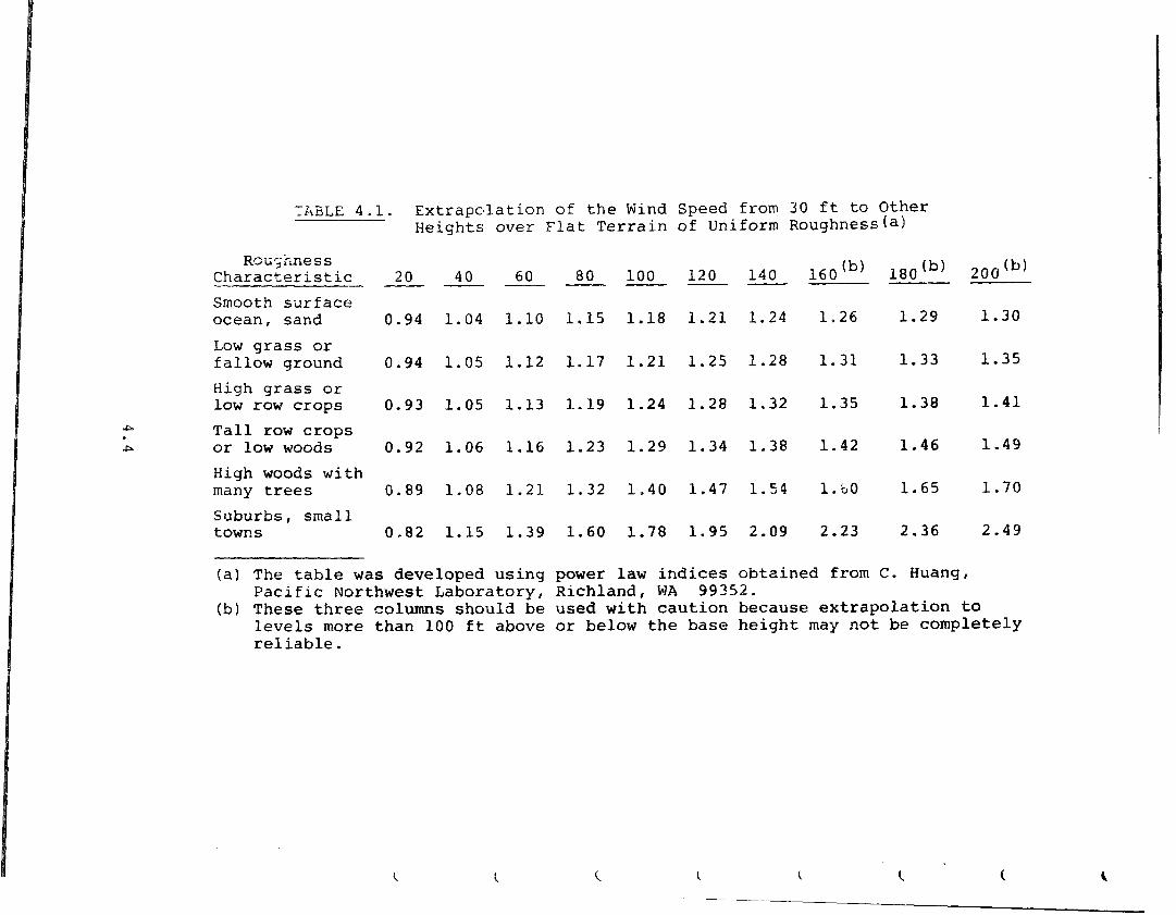
levels. Table 4.1 provides estimates of wind speed changes for

several surface roughnesses at various tower heights. The numbers

IP the table are based on wind speeds measured at 30 ft because

!j:>ti.cnal Weather Service wind data is usually measured at that

nt?iqht. To estimate the wind speed at another level, multiply the

30-ft speed by the factor for the appropriate surface roughness

and height. For example, if the average wind speed at 30 ft over

an area of low grass cover is 10 mph, to determine wind speed at

b0 ft, use the multiplication factor from Table 4.1 (which in this

case is 1.17). Multiply the 10 mph speed by this factor to esti-

!nate the average wind speed at 80 ft: 1.17 x 10 mph = 11.7 mph.

If the height of the known wind speed is not 30 ft, wind

:;_~eec! can be estimated using the following equation:

E Estimated wind speed = K x S

where

I: -1 the table value for the height of the estimated wind

K = the table value for the height of the known wind

S = the known wind speed.

Suppose the 10 mph in the previous example had been measured

dt 20 ft instead of 30 ft. To estimate the speed at 80 ft, divide c kc, .._ 1 . - factor fnr 8@ ft (1,171 by the factor for 20 ft (0.94) to

,~bta:n the corrected factor (1.24); then multiply this corrected

’ act:111- b.?, the known wind speed (10 mph) to estimate the 80-Et wind ';;wE‘il ( : 2 . 4 rll['h) . 'i'h i s ::alculation is shown in equation form ;,I> I !?W (\I:-;! IIt; i!~c* t*cll.icIt ioll above) :

I :; 1 . I7 Ii s i) . 'j-41 s 10 nlI,h - 1.24 x 10 mph = 12.4 mph

4.3

TkELE 4.1. Extrapcllation of the Wind Heights

.b . P

Rouc;iness Characteristic 20 40 -- Smooth surface ocean, sand 0.94 1.04

Low grass or fallow ground 0.94 1.05

High grass or low row crops 0.93 1.05

Tall row crops or low woods 0.92 1.06

High woods with many trees 0.89 1.08

Suburbs, small towns 0.82 1.15

(a) The table was developed

over Flat Terrain

60 80 100 --

1.10 1.15 1.18

120 140 --

1.21 1.24

1.12 1.17 1.21 1.25 1.28

1.13 1.19 1.24 1.28 1.32

1.16 1.23 1.29 1.34 1.38

1.21

1.39

using

1.32 1.40

1.60 1.78

1.47 1.54

1.95 2.09

power law indices obtained from C. Huang, Richland, WA 99352. used with caution because extrapolation to or below the base height may not be completely

Pacific Northwest Laboratory, (b) These three columns should be

levels more than 100 ft above reliable.

Speed from 30 ft to Other of Uniform Roughness(a)

1826 1.29 1.30

1.31 1.33 1.35

1.35 1.38 1.41

1.42 1.46 1.49

1.60 1.65 1.70

2.23 2.36 2.49

'iTable 4.2 cjit'es available wind power changes between levels. (a) -- .-

.rf the height of the known wind is 30 ft, the percentage change of

available power between this level and another can be read directly

from the table. If the known height is other than 30 ft, this equa-

tion can be used to compute the available power change:

Fractional Power Change = lEO-+KK

where

E = the table value for the estimated wind height

K = the table value for the known wind height.

c:~~rnputinq t!?~ available power change for the previous example (i.e.,

~*str~polat~n(l fl.om 20 rt II~ t-o 80 ft over low qrass) , K is -17,

I: is 60. 'I'he fractional L)OWCL' change is:

E-K 60 - t-17) 60 I- 17 77 = = = 100 -t K 100 + (-17) 100 - 17 8-5

= o.93

To express the available power change as a percent, simply multiply

by 100 (0.93 x 100 = 93% increase in available power by raising the

WECS' from 20 ft to 80 ft above a low grass surface).

The heights in Tables 4.1 and 4.2 should not always be thought

of as heights above ground. Over areas of dense vegetation (such

.+:; ;\n orchard or forest) a new "effective ground level" is estab-

lished at approximately the height where branches of adjacent trees

touc11. Below this Level there is little wind; consequently, it is

galled the Icvel of zero wind. In a dense corn field the levei of -__--_-_--.____ ;:<.!rr; wi:lcl w:j~lcl be the average corn height; in a wheat field, the

zverage heic;ht 0;‘ the .&heat, etc. The height at which this level

occurs is c-ailed the "zero displacement height," and is labeled '1 j '1 1p. Fi.liirc> 4.2. !f "d" is less than 10 ft, it can usually be

i L-l ) r\vallablc~ wind power should be used only to compare Sites, not to cstin:+tc ouput power because no WECS can harness all avail- -j5ic: power . I

4.5

Characteristic Roughness

Smooth surface

Low grass

High grass

Tall row crops

High woods

Suburbs

(a) The user is

TABLE 4.2. Power Change Due to Extrapolation to a New Heightta) (Base Height = 30 ft)

20 40 60 80 100 120 - - - - - -

-17 12 33 52 64 77

-17 16 40 60 77 95

-20 16 44 69 91 110

-22 19 56 86 115 141

-30 26 77 130 174 218

-45 52 169 310 464 641

likely to be using National Weather Service (NWS) most NWS wind data is measured at about 30 ft, that level was chosen as the base height for this table. from C. Huang,

The table was developed using power law indices obtained Pacific Northwest Laboratory, Richland, WA 99352.

(b) These three columns should be used with caution because extrapolation to levels more than 100 ft above or below the base height may not be completely reliable.

140 1601b)

91 100

110 125

130 146

163 186

265 310

813 1009

115 120

135 146

163 180

211 231

349 391

1214 1444

wind data. Since

LEVELOF ZERO WIND

VIRTUALLY NO WIND INTHIS REGION

1

FIGURE 4.2. Formation of a New Wind Profile Above Ground Level

disregarded in estimating speed and power changes. However, if

ground level is used when I'd" is actually 10 ft or more, changes

in speed and power from one level to another will be underestimated.

Tables 4.1 and 4.2 express all heights above the "d" height, rather

than above ground.

4 :2 CHANGES IN ROUGHNESS

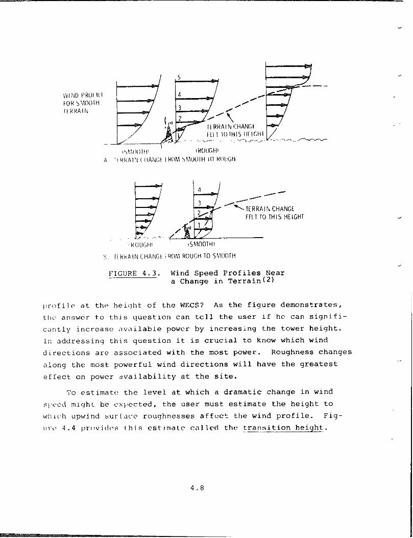
Often roughness varies upwind of the WECS. Figure 4.3 shows

hew a sharp change in roughness affects the wind profile. If a

:L‘FCS were si%ed at the first level in Part A of this figure, the

:.-ier xcu1.d be greatly underutilizing wind energy, since roughness ': il. " ;1." 2 $ cause 3 sharp increase in wind speed slightly above the .: ._ - + _ ; e '7 e 1 . Part B of the figure shows that in smooth terrain

. . /. :-t : .=l AL I if any?hlrlg , wou.ld be gained by increasing tower height

'-l;rf t-cc first ;.evpl. kc even as high as the third. One principle

.;?31idi out: The user will gain more in terms of available power - _-- - - 1-4-~jc:re2s ina , rhe height of a WECS tower located in rough terrain

'.-.??I he will b-1 increasing the height in smoother terrain. ----

a-lcn 3 Lt. i F.0; :L n areas of varying roughness, determining the .,' 1 7 ‘. 1 : 3 r Lilt? !?e17ht I!ri>rn those measured at another presents a new

, a ,- L I '-'.I; : Wk. 1; !I :ipwlnd surface roughness is influencing the wind

4.7

/

\ It RHAI N CHANC t ff.1 I IO THIS tlFIc,til

I.,,--. __

FELT TO THIS HEIGHT

H. It HHAIN CHANGt. I ROM ROUGH TO ShlOOTH

FIGURE 4.3. Wind Speed Profiles Near a Change in Terrain(z)

profile at the height of the WECS? As the figure demonstrates,

tllL: answer to this question can tell the user if he can signifi-

cantly increase available power by increasing the tower height.

In addressing this question it is crucial to know which wind

directions are associated with the most power. Roughness changes

along the most powerful wind directions will have the greatest

effect on power availability at the site.

To estimate the level at which a dramatic change in wind

syecd mlqht be csk,ected, the user must estimate the height to

w2licyh upwind surfarc roughnesses affect the wind profile. Fig- III-~' 4.4 provitl(>s lhis estlmatc called the transition height. _. __ .__

4.8

*;I ;;;'",',",:,""'A"

c- HIGH GRASS

d - TALL ROW CROPS

IT - HIGH WOOS

I SURIIKH5

OiiTA”J: f D<lLVN i’rIN0 iK(l’,\ (.HAYGt It TfRRAIN, FEET

iU KtAD iHI LKAI’H

*if IHtSf lfKkdiNCIAS51tICATIOU~ DO WI APPi b FXACTLY. SEIFCT Iti1 O’J! YARILaI TO Itif RCil~r,tiF\;i‘,(, IiFIT.HT OF Ttif ACTUAL Tt RRAliJ

FIGURE 4.4. Transition Height in Wind Speed Profile Due to a Change in Roughness(2)

The diagram in Figtire 4.5 shows how data from Figure 4.4 can

be used to take advantage of transition height. Since the terrain

cha;qes from an upwind "a" (water) to a downwind "b" (low grass)

ro;lghncss F the upper portion of Figure 4.4 shows that curve I :;;!c;ui;f l;e used. C*iYve 1 in the graph indicates that the transi-

/ I',!-2 tlPl:!!:t at 500 ft Downwind of the shoreline is about 40 ft :~io'.'~' t ilf? :JrrJU!IIl. !;inc*c the smoother surface (water) is upwind,

4.9

PREVAILING POWER.-/ DIRECTION

LOWGRASSLAND ("b" ROUGHNESS)

I*‘1 GUIIrc 4 . 5. F:xamplc of a Transi Lion Iieiqht Diagr;im Depicting Cne Change in Roughr.ess

wind speed should increase sharply around the 40-ft level, 500 ft

downwind from the roughness change. In this example, the WECS

should be located above the transition height because that location

has more available power. Had the rougher surface been upwind,

there would be less to gain by locating the WECS above the transi-

tion height.

The transition height curves in Figure 4.4 are simplified

arlproxirr.ations of a very corr.plex phenomenon. Gradual rather than

stl,rt-p roucfhncss changes may cause the transition to occur in a

!#~yc!r of 10 to LO ft or more J-;lther ttl;ln at a distinct level.

Corlse~lucntly, tllo information in this section should be used orlly

tr) make estimates of +hc wind profile, which then can be used to

select possible WECS sites and tower heights. The best way to l.yerify the wind profile near a change in terrain roughness is to

:-;;A~c a few wind measuremer,ts at various heights during prevailing w : :: ;+ .‘ ‘> ri :?i i LL 1 0 1; F, ? ,h, e i 3 F . L..,o~mafren CIY.. in fh4r .-r.*.d section will help deter- iii; ,;l.f? whcrc to take these mc>;\surements to gain the most useful

i II f L~,rr:~~~t:ion about t.hc willd.

Y

4.10

4. 3 ~3;;.~~.‘iit;:ES I N :t‘L.kT "FHRAIN _ ^ . _ _ _. _-. ._ - . - . -.-,_ .._. _.--. -

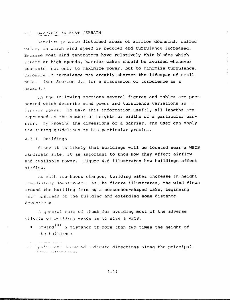
:>arr i F-r.5 ftrC~ci--~re dis -t.Jrbed areas of airflow downwind, called

+./ 2 ;. z :-: , i ri $;!;I c;-, wj, r&d c-p& L - is reduced and turbulence increased.

Recazsn mst wind generatcrs have relatively thin blades which

rotate at high speedss barrier wakes should be avoided whenever

;;(:.s: s j 5 if? , not only to maximize power, but to minimize turbulence.

::sFos\ire to turbulence may greatly shorten the lifespan of small

WECS * (See SectIon 3.1 for a discussion of turbulence as a

hdZdrli. 1

In the following sections several figures and tables are pre-

sented which describe wind power and turbulence variations in .

“2~1 I ?r wakes. L To make this information useful, all lengths are

('xprcssed as the number of heights or widths of a particular bar-

rier. Ey knowing the dimensions of a barrier, the user can apply

the siting guidelines to his particular problem.

3.3.1. Buildings -~

Sll,ce it is likely that buildings will be located near a WECS

candidate site, it is important to know how they affect airflow

and available power. Figure 4.6 illustrates how buildings affect

;Ilrfl9w.

As with roughness changes, building wakes increase in height

1 aI;* cj i ,7 tc> 1 y downs t.rLtam. As the figure illustrates, the wind flows

.:.rou!-1~1 the! hul I(li nq forming a horseshoe-shaped wake, beginning : 11 5 t- ;r~stream of the building and extending some distance

,;i>'&fI.? c :-t'.ll".

.‘I %jc:n.erai I-uie of thumb for avoiding most of the adverse

~fftcts ef bul Iding wakes is to site a !^!ECS:

88 t3pwind'd) - cl distance of more than two times the height of -. i ) P t - t311 i 3 d : nq ;

3 . : ‘.a I :,., ,ii; i<:,.‘,;i:‘: r;,‘, indicate directions along the prii7cLpal : "':,;(; 1 ; , Vi',‘! ; : ,y .

4.11

OUTER LIMIT OFBUILDINCWAKE

FIGURE 4.6. Airflow Around a Block Building (11)

downwindta) a minimum distance of ten times the building

height; or

@ at least twice the building height above ground if the WECS

is to be mounted on the building.

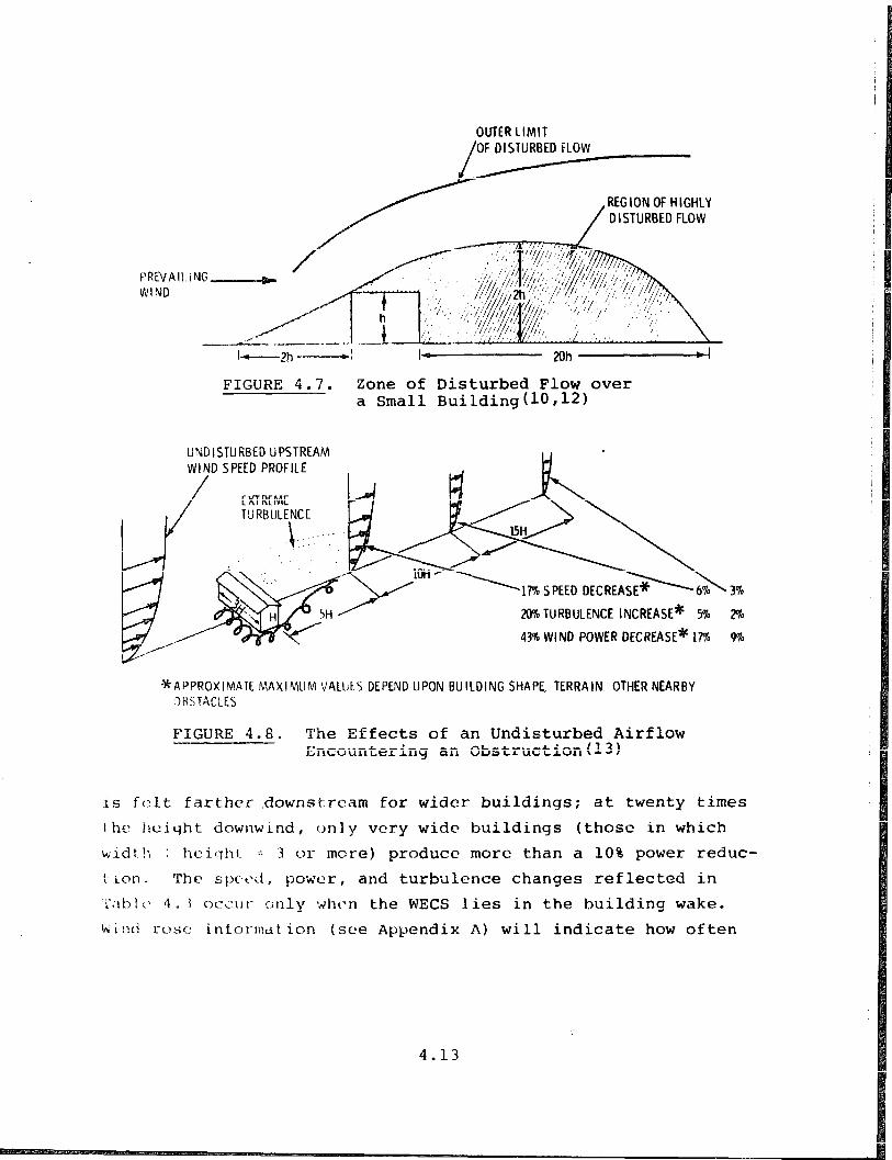
Figure 4.7 illustrates this rule with a cross-sectional view of

the flow wake of a small building.

The above rule of thumb is not foolproof, because the size of

the wake also depends upon the building's shape and orientation to

the wind. Figure 4.8 estimates available power and turbulence in

the wake of a sloped-roof building. All of these estimates apply at a level equal to one building height above the ground. Down- wind from the building, available power losses nearly vanish at a distance equal to 15 building heights.

Table 4.3 summarizes the effects of building shape on wind

speed f availahJe power, and turbulence for buildings oriented per- ~lc~ndicular to the wind flow. Building shape is given by the ratio ":Jidt!; d; VidPd L)\. height . " As might be expected, power reduction

___ -.-.- - - _ - (a) Upwind and downwind indicate directions along the principal

power direct;on.

4.12

OUTER LIMIT OF DISTURBED FLOW

REGION OF HIGHLY DISTURBED FLOW

C’REVAI!.ING~- WI ND

I-zh------d 2Dh -

FIGURE 4.7. Zone of Disturbed Flow over a Small Building(l0,12)

ISTURBED UPSTREAM D SPEED PROFILE

Kf?iTURBULENCE INCREASE* 5% 2%

43% WIND POWER DECREASE* 1% 9%

*APPROXIMATE MAXIMUM VALUES DEPEND UPON BUILDING SHAPE, TERRAIN OTHER NEARBY OBSTACLES

FIGURE 4.8. The Effects of an Undisturbed Airflow Encountering an Obstruction(l3)

is f(:lt farther ,downstrcam for wider buildings: at twenty times

I hc t!eiyht downwind, only very wide buildings (those in which

w i d t !; : hc i 1.~11 t_ 7 3 UT more) produce more than a 10% power reduc-

t- ion. The spc.txi, power, and turbulence changes reflected in i'cib 1 i' 4 . i cYlci111- ijnly *nrhc\n the WECS lies in the building wake.

h’il>ti TI.)SC inforlildtion (see Appendix A) will indicate how often

4.13

4 36 -4 23 14 36 ; 5 14 1

3 24 5 G> 15 11 29 5 4 12 0.5

i 11 -+ 1 5 13 1 i 6 --

0.33 2 .> - . .3 2. 5 1.3 4 0.7; -- -- --

0.25

i:clqht of the i a 7 ‘2 f low rey 1 c.,: +-r. sJildlnq nelyhts)

2 6 2.5 1 3 0.50 me -- --

__.-._- - -_ -.-_ __~ _.__ __ -.--- -

!. 5 2.0 3.0

TABLE 4.3. Wake Behavior of Variously Shaped Buildings (13)

-5, .-’ .A. 7

,

f c

this actually occurs. Annual percentage time of occurrence multi-

plied by the percentage power decrease in the table will give the

net power ioSs. An example of such a calculation is given in

Section 4.3.3.

'If a tower is located on the roof of a building, the turbu-

lence near the roof should be considered. A slanted roof produces

Less turbulence than a flat roof and may actually increase the

wind speed over the building. The zone of speed increase may

extend up to twice the building height if the building is wider

than it is tall and is oriented perpendicular to the prevailing

wind. However, since wide buildings are generally not very high,

the roof is only exposed to the lower wind speeds near the ground.

Rather than attempting to use the power in the wind accelerated

over such a building, it is generally wiser to raise the WECS as

h:.gh as is economically practical, taking advantage of the fact

that winds usually increase and turbulence decreases with height.

4.3.2 Shelterbelts

Shelterbelts are windbreaks usually consisting of a row of

trees. When selecting a site near a shelterbelt, the user should

cithc:r

* choose a site far enough upwind/downwind to avoid the dis-

t-urbcd flow;

* use a tower of sufficient height to avoid the disturbed flow;

or

e if the disturbed flow at the shelterbelt cannot be entirely

(avoided, minimize power loss and turbulence by examining the

nature of the windflow near the shelterbelt and choose a site

L3ccordinqly.

‘I’hl~ til‘q 1 I’(’ to which t-he wind flow is disturbed depends on the

'l~‘l~!lll , lr~~!~~tl~, ,111,1 \hjr-c>:: ity of the shelterbelt. Porosity is the I *II 14 01 IllI: ll,~"ll ,I1 I',1 III A winclbrcl,lk to the total area (expressed !l: !L' .iS t !I<> ~N~~~~~c~I~C~CJP of open area) .

:.15

Figure 4.9 locates the region of greatest turbulence and wind

speed reduction near a thick windbreak. How far upwind and down-

wind this area of disturbed flow extends varies with the height of

the windbreak. Generally, the taller the windbreak is, the farther

the region upwind and downwind that will experience a disturbed

airflow.

Figure 4.10 illustrates the effect of a row of trees on the

wind speed at various heights and distances from the windbreak.

The wind speeds are expressed as percentages of undisturbed upwind

flow at several selected heights. All heights and distances are

expressed in terms of the height of the shelterbelt to make appli-

cation to a particular siting problem easier.

When examining this figure, the reader should note that loose

foliage actually reduces winds behind the windbreak more than dense

foliage. Furthermore, medium-density foliage reduces wind speeds

farther downwind than either loose o.r dense foliage.

For levels l-l/Z H or less, the wind speed begins to decrease

at 5 or 6 H upstream of the shelterbelt. Therefore, if the shelter-

belt is 30 ft high and the WECS tower is only 45 ft high, the site

should be at least 150 ft (5 H) upstream of the windbreak to

entirely av0i.d the speed decrease and turbulence on the windward

side.

d-

WI RlDWARD

d

J

J

FIGURE 4.9. Airflow Near a Shelterbelt(12) _-------

4 .l(l

WINDBREAK

No

80

OL------- lo 5 0 5 la 15 20 25 30

HORIZONTAL DISTANCES INMULTIPLESOFH (H = HEIGHT OFTHEWINDBREAK)

(a'COLORADO SPRUCE-TYPE TREE

'b'PINE TYPE TREE

FIGURE 4.10. Percent Wind Speed at Different Levels Above the Surface Behind a Row of Trees of Height, H(l2)

At a distance of 2-l/2 H downwind, the wind speed at the

2-l/2 M level (for both dense and loose foliage) increases approxi-

~te1.y 5% . At first glance this appears to be a good WECS site.

iirWeVc r , there is a turbulent zone downwind from the shelterbelt

that may make this site undesirable, particularly if the tower is

t LX> short. Figure 4.11 shows this zone of turbulence.

'1'0 capitalize on the acceleration of the wind over a shelter- 17.~ i t , the> entire r-rotor disc must be located above the turbulent

a Lr)ne. To determine where this turbulent zone is located, the user

should study turbulence patterns during prevailing wind conditions.

4.17

4

TOP OF TURBULENT REGION

(IN TERMS OF SHELTER- 3 BELT HE I GHT)

. . . . .

I -- l 1 I _- -- t

1 0 10 20 30 40

SHELTERBELT DI STANCE DOWN WIND (HEIGHTS OF SHELTERBELT!

FIGURE 4.11. The Zone of Turbulence Behind a Shelterbelt

(Section 3.1 presents simple methods of turbulence detection.) He

should also study other frequently occurring wind directions. If

significant turbulence or power loss is possible when the wind

blows from the most powerful directions, another site should be selected.

?';lblc 4 . 4 provides information on the wind speed/availabie power reductions and turbulence increases for sites in the lee of

the shelterbelt. Speed, power, and turbulence changes are expressed as upwind percentages. The porosity of the windbreak can be estimated visually, then Table 4.4 can be used to determine how far downwind the site should be located to minimize power loss

and turbulence. Speed, power, and turbulence changes expressed in the tabie occur only when the WECS lies in the shelterbelt wake.

W i nil rose inform;lt.ion (set Appendix A) will indicate how often

I- 11 is ;l<*tllcllly occ-urs. ,\n~l\i~~l percentaqis time of occurrence multi- 111 icci l)y the> t~tL)l~~ Iwr-c:cnt.,lye will (~ivc! 1 he net change. An example ,I< this t.ytjc of calc.uLation is yiven in t.h(: following section.

.

.

a

- .

J

. -

.

4.18

TABLE 4.4. Available Power Loss and Turbulence Increase Downwind from Shelterbelts of Various Porosities(l3)

Downwind Distances (In Terms of Shelterbelt Heights) ___-.-- 5H 10H 2011 ------ -- -

(a) Percent Percent Percent Percent Percent Percent Percent Percent Percent

Porosity Speed Power Turbulence Speed Power Turbulence Speed Power Turbulence m Area : Total Arear Decrease Decrease Increase Decrease Decrease Increase Decrease Decrease Increase ---- -- -- __--.-.. _____

00 (nc; space between trees)

40 78 ia 15 39 18 3 9 15

20%

(wrth loose foliage such as pine or broadleaf trees)

a0 99 9 40 78 -- 12 32 --

40%

Lwlth dense foliage such as Colorado Spruce)

70 97 34 55 90 -- 20 49 --

-

To11 of Turbulent Zone (in terms of shelter&It height)

2.5 3.0 3.5

(a) Determine the porosity category of the shelterbelt by estimating the percentage of open area and by associating the foliage with the example tree type.

4.3.3 Individual Trees

The trees near a prospective WECS site may not be organized

into a shelterbelt. In such cases the effect of an individual

tree or of several trees scattered over the surrounding area may

be a problem.

The wake of disturbed airflow behind individual trees grows

larger (but weaker) with distanee, much like a building wake.

However, the highly disturbed portion of a tree wake extends far-

ther downstream than does that of a solid object. Table 4.5 may

be used to estimate available power loss downstream. For example, consider a 30-ft wide tree having fairly dense foliage. At 30 tree widths (or 900 ft) downstream, the table indicates a 9% loss of available power whenever the WECS is in the tree wake. The

d numbers in the bottom two rows of the tabie provide estimates of

the width and height of the tree wake. The velocity and power

losses expressed in the table occur only when the WECS lies in the

tree wake. J

TABLE 4.5. Speed and Power Loss in Tree Wakes (13)

Distance Downwind (In Tree Widths) 5 10 15 -.-.-- - ---

Dense-fol iaqe tree\ Maximum percent (such as a Colorado loss of velocity 20 9 6 spruce) Max imum percent

loss of power 49 25 17 Thin-foliage tree Msximum percent (such as a pine) loss of velocity 16 7 4

Maximum percent loss of power 41 18 12

Height of the turbulent flow region (in trcxc heights) 1.5 2.0 2.5

EL'1,lt.h ui turbulent flow region (:I) tree widths) 1.5 2.0 2.5

20 30 --

4 3

13 9

3 2

8 6

3.0 3.5

3.0 3.5

4.20

If available, wind rose information (Appendix A) can be used

tc estimate the percentage of time a site will be in the tree

wake, and ',here,by the total power loss due to the tree. For

instance, suppose that 50% of the time the wind direction places

the site in the tree wake. In the example above, the tree pro-

duced a 9% loss of available power. If the loss occurred 50% of

the time, 4.5% (50% x 9%) of the available power would be lost

annually.

4.3.4 Scattered Barriers

The advantages of increasing tower height are evident from

this example, especially if scattered trees or buildings are in

the vicinity. Since choosing a site not located in any barrier

wake will probably be impossible in these areas, the WECS should

be raised above the most highly disturbed airflow. To avoid most of the undesirable effects of trees and other barriers, the rotor

disc should be situated on the tower at a minimum height of three

times that of the tallest barrier in the vicinity. If this rule

is impractical (for economic or other reasons), the user can

1) find the minimum height required to clear the region of high-

est turbulence by using the turbulence detection techniques out-

lined in Section 3.1, or 2) choose the site so that the WECS will

clear the highest obstruction within a SOO-ft radius by at least

25 ft.(l)

4.21

5.0 SITING IN NON-FLAT TERRAIN

any terrain that does not meet the criteria listed in Fig-

ure 4.1 is considered to be non-flat or complex. To select candi-

date sites in such terrain, the Fotential user should identify the

terrain features (i.e., hills, ridges, cliffs, valleys) located in

or near the siting area and then read the applicable portions of

Section 5.

In complex terrain, landforms affect the airflow to some

height above the ground in many of the same ways as surface rough-

ness does. However, topographical features affect airflow on a

much larger scale, overshadowing the effects of roughness. When

weighing various siting factors by their effects on wind power,

topographical features should be considered first, barriers second,

and roughness third. For example, if a particular section of a

ridge is selected as a good candidate site, the location of bar-

riers and surface roughness should only be considered to pinpoint

the best site on that section of the ridge.

Ridges are defined as elongated hills rising from about 500

to 2000 ft above surrounding terrain and having little or no flat

area on the summit (see Figure 5.1). There are three advantages

to locating a WECS on a ridge: 1) the ridge acts as a huge tower;

2) the undesirable effects of cooling near the ground are avoided;

and 3) the ridge may accelerate the airflow over it, thereby

increasing the available power.

The first two advantages are not unique to ridges, but apply

alI toyoyrak>hical features having high relief (hills, mountains, c*tx.). As Section 2.2 points out, winds generally increase with

A ridge, then, like a tower, raises a WECS into a region

In addition, daily temperature changes affect

5.1

1. H = 500T0 2DDO fl

2. L SAT LEAST 10 x H(l"'

3. ROUNDED OR PEAKEDTOP (NOT FLAT)

FIGURE 5.1. Definition of a Ridge

the wind profile. At night as the earth's surface cools, the air

near the surface cools. This cool, heavy air drains from the hill-

sides into the valleys and may accumulate into a layer several

hundred feet deep by early morning. This cool dome of air dis-

engages from the general wind flow above it to produce the cool,

calm mornings that lowlands often experience. Because of this

phenomenon, a WECS located on a hill or ridge may produce power

all night, but one located at a lower elevation may not.

A similar, but more persistent, situation may occur in the

winter when cold air moves into an area. Much like flowing water,

cold air tends to fill all the low spots. This may cause extended

periods of calm in the lowlands while the surrounding hills experi-

race winds capable of driving a WECS.

R\. siting at hiqher elevations, such as on a ridge, the user Lqs~~~ t.lkc ~dv,lnta(l~~ of more persistent winds. And, since a WECS 1 l'l.'L\ t l,ll lJI1 a r icIql1 t'r<~l:~cc!; more encrqy , it can reduce the amount (J I ent~l-~]y stor,lqc c,\pacity needed (such as batteries) and provide

<I IllOrc cle~)cndclL~lc- and economical sourcf: of power.

5 .2

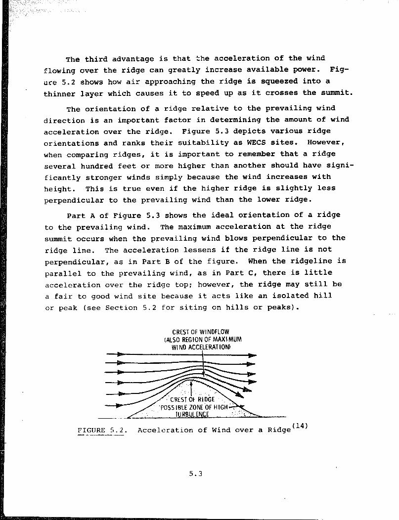
The third advantage is that .Lhe acceleration of the wind

flowing over the ridge can greatly increase available power. Fig-

ure 5.2 shows how air approaching the ridge is squeezed into a

thinner layer which causes it to speed up as it crosses the summit.

The orientation of a ridge relative to the prevailing wind

direction is an important factor in determining the amount of wind

acceleration over the ridge. Figure 5.3 depicts various ridge

orientations and ranks their suitability as WECS sites. However,

when comparing ridges, it is important to remember that a ridge

several hundred feet or more higher than another should have signi-

ficantly stronger winds simply because the wind increases with

height. This is true even if the higher ridge is slightly less

perpendicular to the p--V rev-ailing wind than the lower ridge.

Part A of Figure 5.3 shows the ideal orientation of a ridge

to the prevailing wind. The maximum acceleration at the ridge

summit occurs when the prevailing wind blows perpendicular to the

ridge line. The acceleration lessens if the ridge line is not

perpendicular, as in Part B of the figure. When the ridgeline is

parallel to the prevailing wind, as in Part C, there is little

acceleration over the ridge top; however, the ridge may still be

a fair to good wind site because it acts like an isolated hill

or peak (see Section 5.2 for siting on hills or peaks).

CREST OF WINDFLOW (ALSO REGION OF MAXI MUM

Wi ND ACCEJmERATION)

-._. - __

FIGURE 5.2. Acceleration of Wind over a Ridge (14) -.-

5.3

ORIENTATION

A. PERPENDICULAR (BEST) 6. OBLIQUE (GOOD) C. PARALLEL (FAIR)

SHAPE

D. CONCAVITY lGO@DI E. CONVEXITY (LESS DESIR<ABLETHANCONCAVEI

FIGURE 5 . 3 . The Effects of Ridge Orientation and --- Shape Upon WECS Site Suitability

The orientation of concave or convex ridges (or such portions

of a ridqc) can further modify the wind flow. Part D of Figure 5.3

shuws how concavity on the windward side may enhance acceleration

over the ridge by funneling the wind. On the other hand, convexity

on the windward side (Part E) reduces acceleration by deflecting

the wind flow around the ridge.

Figure 5.4 shows the cross-sectional shapes of seve.fal ri.dc;ei;

and ranks them by the amount of acceleration they produce. Notice +hDt . ..*u L ;. triaiiyuiar-shaped ridge causes the greatest acCe~erati@n,

and that the rounded ridge is a close second. The data used In

ranking these shapes were collected in laboratory experiments using

wind tunnels to simulate real ridges. Though few wind experiments

have been conducted over actual ridges, the results are similar to

t\li~nel simulations. Both indicate that certain slopes, primarily

111 the tle‘lrc:;t 1-c-w llundrcd yards to the summit, (aI increase the ..-_ .-_~ --

-- -- -_--_ (;1) This portion c?f the ridqc has the greatest influence on the

witId l‘rofilc\ immediately above the summit.

. -

5.4

1. TRIANGULARMOSTACCELERATlONl 2. ROUNDED

3. FLATTOP 4. STEEP SLOPE

5. BLUFF (LEAST ACCELERATION) l

FIGURE 5.4. Ranking of Ridge Shape by Amount of Wind Acceleration(l1)

, wind more effectively than others. Table 5.1 classifies smooth,

regular ridge slopes according to their value as wind power sites.

Figure 5.5 gives percentage variations in wind speed for an

ideally-shaped ridge. Since these numbers are taken from wind

tunnel experiments, they should not be taken too literally: never-

theless, the user should expect similar windspeed patterns along

the path of flow. Generally, wind speed decreases significantly

at the foot of the ridge, then accelerates to a maximum at the

ridge crest. It only exceeds the upwind speed on the upper half

of the ridge.

Another consideration in choosing a site on a ridge is the

turbulent zone which often forms in the lee of ridges (Figure 5.2).

The stet?per the ridge slope and the stronger the wind flow, the

more l.ih,cly turbulence will form in the lee of the ridge. Thus, it is safest to site at the summit of the ridge, both to maximize

[rower sn:! to <Ivoid Lee turbulence.

TABLE 5.1. WECS Site Suitabilit Slope of the Ridget 5 )

Based Upon

WECS Site Suitability Ideal

Very good Good

Fair

Avoid

Slope of the Hill Near the Summit

Percent Slope - Grade(a) Anule ----

29 160

17 lo0 10 6O

5 3O

less than 5 less than 3" greater than 50 greater than 27*

(a) Percent grade as used above is the number or‘ feet of rise per 100 ft horizontal distance.

FIGURE 5.5. Percentage Variation in Wind Speed ~-- over an Idealized Ridgef2)

Shoulders (ends) of ridges are often good WECS sites. Eve:':

for a very long ridge, as much as one-third of the air approaching

at low levels may flow around, rather than over, the ridge. (21 To

move such a volume of air around the ridge, the wind must acceder-

ate as it flows around the ends. No quantitative estimates of thi$,

acceleration are available at this time, but it appears that from

the standpoint of available wind power the ends of ridges may :.srlk

second behind the ridge crest as the best potential WECS sites.

Flat-topped ridges present special problems because they can

actually create hazardous wind shear at low levels, as Figure 5.6

illustrates. Consequently, the slope classifications used in

Table 5.1 do not apply to these ridges. The hatched area at the

top of the flat ridge indicates a region of reduced wind speed due

to the "separation" of the flow from the surface. Immediately

above the separation zone is a zone of high wind shear. This shear

zone is located just at the top of the shaded area in the figure. Siting a WECS in this region will cause unequal loads on the blade

ds it. rotates through areas of different wind speeds and could

decrease performance and the life of the blade. The wind shear

problem can be avoided by increasing tower height to allow the

blade to clear the shear zone or by moving the WECS toward the

windward slope.

SPEED-UPCAUSED BY THERIDCE

I REGIONOF HIGH

SPEED IS REDUCED INTHIS DCE InN IN IF Tn TUF FI AT nL" IvIm ""L I" II 1- SURFACE

FIGURE 5.6. Hazardous Wind Shear over a Flat-Topped Ridge --

5.7

As in the case of flat terrain, the effects of barriers and

roughness should not be overlooked. Figure 5.7 shows how a rough

surface upwind of a ridge can greatly decrease the wind speed.

After selecting the best section of a ridge based upon its geometry,

the potential user should consider the barriers, then the upwind

surface roughness.

The most important considerations in siting WECS on or near

ridges are summarized below:

1) The best ridges or sections of a single ridg,e are those most

nearly perpendicular to the prevailing wind. (However, a

ridge several hundred feet higher than another and only

slightly less perpendicular to the wind is preferable.)

2) Ridges or sections of a single ridge having the most ideal

slopes within several hundred yards of the crest should be

selected (use Table 5.1). Ridge sites meriting special

consideration are those with features such as gaps, passes,

or saddles (Sections 5.3 and 5.4).

WIND SPEED

ROUGH SURFACE

z c3 lzi I: SMOOTH SURFACE

J

I'IG'JRE 5.7. Effect of Surface Roughness on Wind Flow - ~--- over a 1,o.w Sharp-Crested Ridqetll)

/

3)

4)

5)

6)

5.2

Sites where turbulence or excessive wind shear cannot be avoided should not be considered.

Roughness and barriers must be considered.

If siting on the ridge crest is not possible, the site should be either on the ends or as high as possible on the windward slope of the ridge. The foot of the ridge should be avoided.

vegetation may indicate the ridge section having the strong- est winds (Section 5.9).

ISOLATED HILLS AND MOUNTAINS

An isolated hill is 500 to 2000 ft high, is detached from any ridges, and has a length of less than 10 times its height. Hills greater than 2000 ft high will be referred to as mountains.

Hills, like ridges, may accelerate the wind flowing over them but not as much as ridges, since air tends to flow around the hill (Figure 5.8). Not enough information is currently available to make quantitative estimates of wind accelerations either over or around isolated hills. However, Table 5.1 can be used to rank hills according to their slope.

Two benefits are gained by siting on hills: 1) airflow can be accelerated, and 2) the hill acts as a huge tower, raising the WECS into a stronger airflow aloft and above part of the nocturnal cooling and resulting calm periods.

The best WECS sites on an isolated hill may be along the sides of the hill tangent to the prevailing wind (shown as hatched areas in E'igure 5.8). (11) However, further research is required to verify this supposition. Currently, simultaneous wind recordings are the surest method of comparing hillside and hilltop sites.

Table 5.2 ranks the suitability of WECS sites on hills. How- C'VE!!I‘ , the effects vf surface roughness and barriers should also be wc-iqhod before a WECS site is selected.

5.9

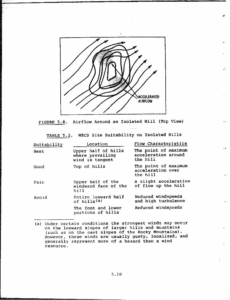
FIGURE 5.8. Airflow Around an Isolated Hill (Tcp View)

TABLE 5.2. WECS Site Suitability on Isolated Hills

Suitability Location

Best Upper half of hills where prevailing wind is tangent

Good Top of hills

Fair Upper half of the windward face of the hill

Avoid Entire leeward half of hills(a)

The foot and lower portions of hills

Flow Characteristics ---ulye The point of maximum acceleration around the hill

The point of maximum acceleration over the hill

A slight acceleration of flow up the hill

Reduced windspeeds and high turbulence

Reduced windspseds

-I

(a) Under certain conditions the strongest winds may occur cn the leeward slopes of larger hills and m6clntains (such as on the east slopes of the Rocky Mountains). However, these winds are usually gusty, localized, and generally represent more of a hazard than a wind resource.

When choosing a site on isolated mountains, the potential user

should consider all the factors discussed for hills. However,

because of the greater size, greater relief, and more complex ter-

rain configurations of mountains, other factors must be considered.

Inaccessability may create logistical problems, and thunderstorms,

hail, snow, and icing hazards will occur more frequently than at

lower elevations.

in spite of the drawbacks, an isolated mountain may still be

the most promising WECS site in an area. To select the best site(s)

in the favorable areas of the mountain, use the criteria for hills

in Table 5.2. For mountains, these favorable areas may be very

large, containing many different terrain features, barriers, and

-surface roughnesses. To pinpoint the best site(s), consider the

largest terrain features first; then evaluate the barriers and sur-

face roughness.

5.3 I'ASSES AND SADDLES ----

Passes and saddles are low spots or notches in mountain bar-

riers. Such sites offer three advantages to WECS operations.

First, since they are often the lowest spots in a mountain chain,

they are more accessible than other mountain locations. Second, hccaUSe they are flanked by much higher terrain, the air is fun-

r!clcd as it is forced through the passes. Third, depending upon the steepness of the slope near the summit, wind may accelerate

over the crest as it does over a ridge.

Factors affecting airflow through passes are orientation to

the i)revai.ling wind, width and length of the pass, elevation dif-

t~1:'rc!:Ic'cs bctwcon the pass and adjacent mountains, the slope of : !:~a (dss ncdr t.llt> crest , and the surface roughness. At this time, t.hetc? has not been sufEi.cient research to allow classification of !j 1; c s :;ltc suit&iLity in terms of these factors. However, some ?iL‘S I I AIL>! ,' 4-'l~,lr‘1(‘tc1~-ist its of passes are listed below:

5.11

z

.

4

1)

2)

3)

4)

the pass should be open to the prevailing wind (preferably

parallel to the prevailing wind);

the pass should have high hills or mountains on both sides

(the higher the better);

the slope (grade) of the pass near the summit should be suf-

ficient to further accelerate the wind like a ridge (see

Table 5.1 for slope suitability); and

the surface should be smooth (the smoother the better). (IF

the pass is very narrow, the user should consider the rough-

ne.;s of the sides of the pass.)

Figure 5.9 shows two views of the wind profiles in a pass.

Part A is a view through the pass. A core of maximum wind (denoted by the innermost circle) is located in the center of the

pass I well above the surface. Part B is looking across the pass.

In this view, a strong increase in wind from the ground up to the

wind maximum is clearly shown. The WECS should be sited near the center of the pass at a level as near the core of maximum winds

as possible. Below this level there may be very strong vertical

wind shear and much turbulence. Since the location of the core will vary from pass to pass, wind measurements are recommended before a final decision on WECS placement is made.

Passes to avoid are those not open to the prevailing wind

(because there will be much less flow through them) and passes,

or portions of passes, which are extremely narrow and canyon-Like

(bccausc these> may have turbulence and strong horizontal wind

shc?ar) .

4

I

4

. -

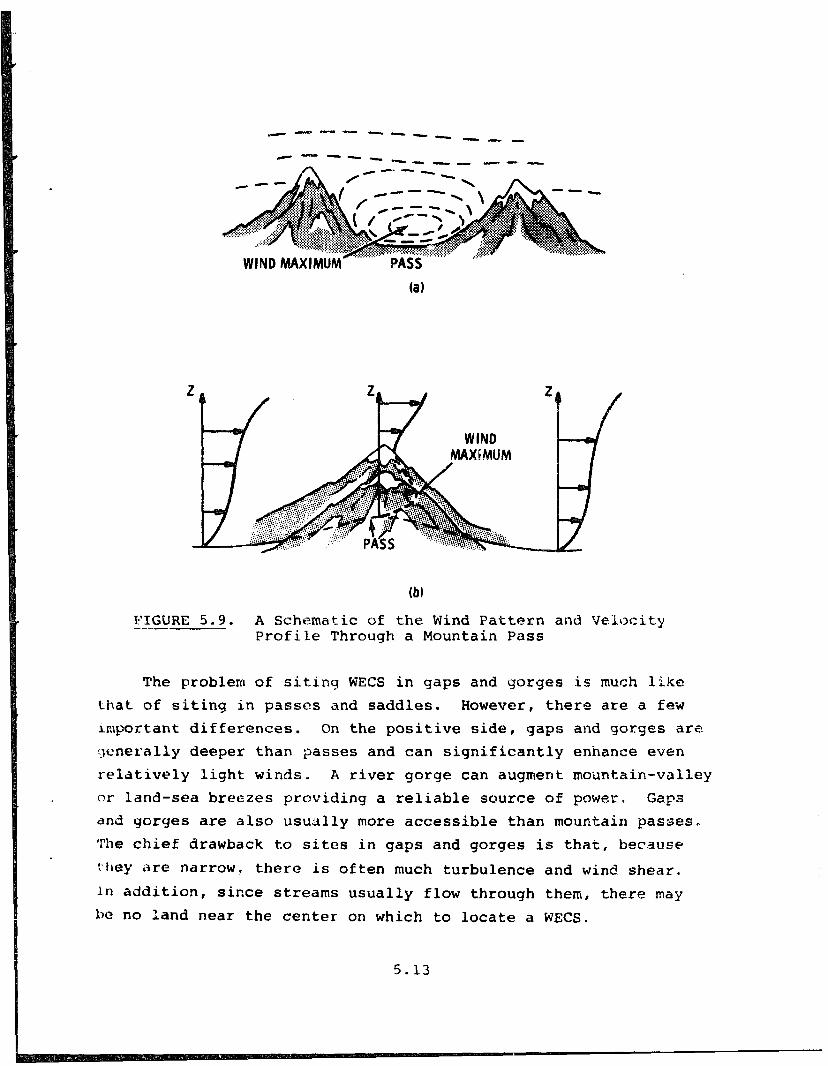
WIND MAXIMUM (a)

FIGURE 5.9. -...- A Schematic of the Wind Pattern and Yelixity Profile Through a Mountain Pass

The problem of siting WECS in gaps and yorges is much like

that of siting in passes and saddles. However, there are a few

important differences. On the positive side, gaps and gorges are

fdenerally deeper than >asses and can significantly enhance even

relatively light winds. A river gorge can augment mountain-valley

or land-sea breezes providing a reliable source of power, Gaps

and gorges are also usually more accessible than mountain passes.

The chief drawback to sites in gaps and gorges is that, because

:-trey are narrow, there is often much turbulence and wind shear.

In addition, since streams usually flow through them, there may

be no land near the center on which to locate a WECS.

5.13

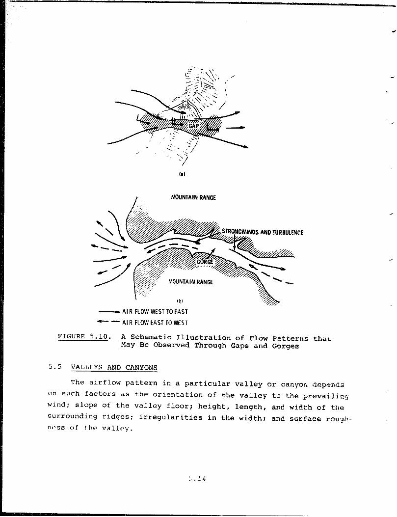
(8)

r MCIUNTA IN RANGE

MQUKTA IN RANGE

- AIR FLOW WEST TO EAST

- - AIR FLOW tAST TO WEST

JRONGWINDS AND TURBULENCE

FIGURE 5.10. A Schematic Illustration of Flow Pirtterns that May Be Observed Through Gaps and Gorges

5.5 VALLEYS AND CANYONS

The airflow pattern in a particular valley or canyon depe?nds on such factors as the orientation of the valley to the ?revailjzc,

wind; slope of the valley floor; height, length, and width of tire surrounding ridges: irregularities in the width: and surface rou#- nc'ss of t-hr, vallr-y.

Valleys and canyons which do not slope downward from moun-

tains are usually Rot gcjod Sites. Perhaps the only benefit to

siting in non-sloping valleys is the possible funneling effect

when the large-scale prevailing wind blows parallel to the valley.

Funneling occurs only if the valley or canyon is constricted at

some point. Unless the vallel; is constricted, the surrounding

ridges will provide better WECS sites than the valley floor.

Three types of flow patterns occur in valley-mountain systems.

'I'hc first , known as valley (mountain)-slope winds, occurs when the

large-scale wind over the area is weak, and the daily hearing and

cooliny cycle dominates. This happens most often during tile warmer

months (May to September).

The daily sequence of vail (mountain)-slope winds is shown

in Figure 5.11. Shortly after sl *ise when the valley is ccld and

the plains are warm, upslope winds (w!litt xrows) and the! continu-

,tion of the mountain winds (black arrows) combine (Part A). At

forenoon when the plains and the valley floor are the same tempera-

ture, the slope winds are strong and there is a transition from

mountain to valley winds (Part B). At noon and during early after-

noon, the slope winds diminish. The valley wind is fuily developed

and the valley is warmer than the plains (Part C). In late after-

I loon , the slope winds cease ~:i; the valley winds continue. The

..~,271 Lc*y is still warmer than the plains (Part D). Shortly after

sunset when the valley is only slScJht1 I warmer than the plains,

downslope winds begin and the valley H' xis weaken (Part Ej. In

c>arly night downslope winds are well developed. The valleys and

plains are at the same temperature. This overall condition is

.rharactcristic of the transition period between valley and moun-

:.\in winds (Part F). In the middle of the night, the valley, is

. xldcr than the plains. Hence, the downslope winds continue and

the mountain wind is fully developed (Part G). From late night

ICI m@rn1ntl when the valley is colder than the plains, downslope h I IKi.~ 4'~‘.\?5C .ind the mountain wind fills the valley (Figure H) .

5.15

(A) SUNRISE (EARLY MORNING) (BI FORENOON

(Cl EARLY AFTERNOON (0) LATE AFIERNOON

(El EVENING (AFTER SUNSET1 (F) EARLYNIGHT ,

(G) MIDDLE OF NIGH1 (HI LATE NIGHT

F-1. :LRE 5.11. -.- -~ l'tx Daily Sequence of Mountain and Valley Winds (Source : Reference 16, reprinted by permission of the American Meteorological Society)

The winds vf c;reatest interest for small WECS users are the

nlc>u;lcain wind at niIlht (l';lrts A, G and II of Figure 5.13.) and the

l.,x1 ity wlr.ci dur?ncl the afternoon (Parts C, D and E) ti Figure 5.12

illustrates a wind profile observed for mountain winds in Vermont.

S'!?L wirld z!c-ccleratcbs down the valley, with the strongest mountain

Is . 1 (j

THIS PROFILE IS BASED UPON A LIMITED NUMBER OF OBSERVATIONS ii\i A SINGLE AREA OF THE UNITED STATES

FIGURE 5.12. Vertical Profile of the Mountain Wind (2)

-- --

winds occurring at the mouth (lower end) of the valley, and the

lightest winds at the head (upper end). In the vertical direz-

tion, the wind speed increases upward from the valley floor and

iids reached a maxrmum in the center of the valley at about two- -- tklrds the height of the surrounding ridges. At the point of --~ maximum wind, the speed may reach as high as 25 mph. The moun-

tain wind is generally well developed for valleys betweenLie

i !dq~zs and/or rather steeply sloping valley floors. The upper -.-- ijalf of the wind profile is very smooth while the lower ha3.f

l>ccasionally becomes qusty and turbulent.

'!-hl. daytime wind blowing up the valley tends to be more sen-

:;I! jiJc> io frl~tc?rs SGC:~ as heating by the sun (the driving force

! !>I t I-1 I s wi~kt 1 .rnL1 Lhcs winds blowing high overhead. As a rc->sult,

5.17

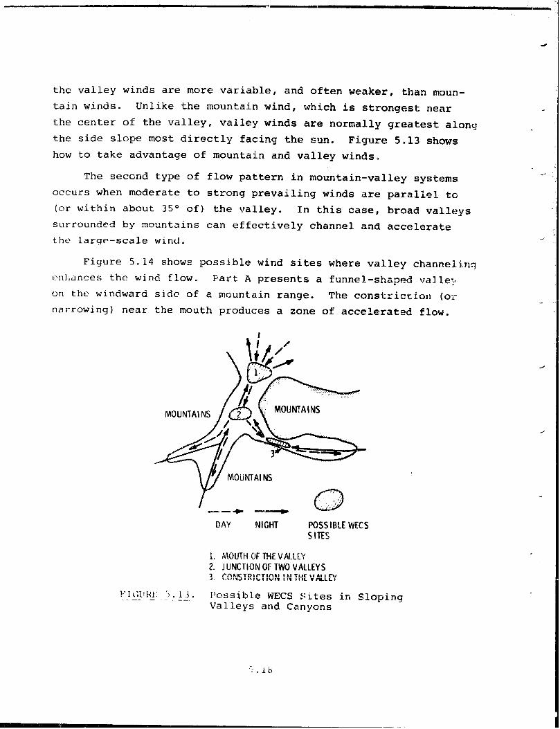
the valley winds are more variable, and often weaker, than moun-

tain winds. Unlike the mountain wind, which is strongest near

the center of the valley, valley winds are normally greatest along the side slope most directly facing the sun. Figure 5,13 shows how to take advantage of mountain and valley winds.,

The second type of flow pattern in mountain-valley systems

occurs when moderate to strong prevailing winds are paraliel to

(or within about 35O of) the valley. In this case, broad valleys surrounded by mountains can effectively channel and accelerate

the large-scale wind.

Figure 5.14 shows possible wind sites where valley channeling t:nl,anres the wind flow. Part A presents a funnel-shaped \ralle:# on the windward side of a mountain range. The constriction (oic narrowing) near the mouth produces a zone of accelerated flow.

I ---a- -4

w

DAY NIGHT POSSIBLE WECS SITES

1. MOUTH OF THE VALLLY 2. JUNCTION Of: TWO VALLEYS 1 ,. Cgp!STra!rTmrd ty IKE vk~yy I*. \r,,“IW II

VI C;llHi: r:. 1 3. Possible WECS Sites in Sloping Valleys and Canyons

;b,

iONE OF ACCELERATED Al RROW

MOUNTA I NS

- ZONE OF HIGH WIND VELOCITIES

75 MILES

PREVAILING WINDS

FTGURE 5.13. possible WECS Sites Where Prevailing Winds are Channeled by Valleys

7 ,- 1 _. chit; ?Xal?.pie, the valley is large (approximately 60 miles wide1 - ._ 2 a. i'i sFen to the prevailiplg wind. Part i3 shows a narrow vailey in

t.hc- ice of a mountain range. It is parallel to the prevailing

.\;.Zd and constricted slightly near its mouth.

A ?:.?lley which is both parallel to the prevailing wind and

.-..:i‘ei- i enccs rnou,i~t~~iri-\~ alLey winds will provide sites which are

~.~-5:?er1ddt)Lc! sources of power. Moderate to strong prevailinq winds

n wylnter and spring will drive the WECS. During the warmer ."'-.t):, t,'-.s , mountain-valley winds can be utilized.

5.19

J

The third type of valley flow occurs when the prevailing wind

is perpendicular to the valley (or crosses it at an angle greater

than 35'). A vailey eddy may be set up by a combination of solar

heating and cross-valley winds. Though there may be times when

this eddy could be exploited by a WECS located on either side slope

of the valley, it is not a dependable power source because it only

occurs on sunny days and is very turbulent.

1)

2)

3)

4)

5)

I, !

7i

i - ,

To site WECS in valleys and canyons, the potential user should

select wide valleys parallel to the prevailing wind or long

valleys extend.ing down from mountain ranges;

choose sites in possible constrictions in the valley or can-

yon where the wind flow might be enhanced;

avoid extremely short and/or narrow valleys and canyons, as

well as those perpendicular to the prevailing winds:

choose sites near the mouth of valley where mountain-valley

winds occur;

insure that the tower i: high enough to place the WECS as

near to the level of maximum wind as is practical;

use vegetation to indicate high wind areas (see Section 5.9);

and

consider nearby topographical features, barriers, and surface

roughness (after favorable areas in the valley or canyon are

located).

t;AS 1 NS -...-

Ba.!al!lS are depressions surrounded by higher terrain. Large c

T<hal?oi< inland basins (such as the Columbia Basin in southeast K.ist! iny ton ) n.;ty have daily wind cycles during the warmer months

Of :he year which can be used to drive small WECS. The flow into

:ci;ci glut of a basin is similar to the mountain-valley cycle in UT i -;cr e 5.11. :!t fact, val!eps sloping dcwn into basins may pro- '\. ! !CJ sufficient ehannelinq to warrant ,;fJ;~s;dczza$--eg 35 \b;r;::>; s; :,, I*

- -.

.

The flow of cool ok- f Porn surrounding mountains and hills

into the basin during tke zkight is usuaily stronger than the flow

out of the basin caused by daytime heating. Well-developed night-

time flow into a basin may average from lo-20 mph for several :

hours during the night, and occasionally more than 25 mph for

periods of one or two hours. Afternoon flow out of the basin is

generally lighter, averaging f-15 mph.

Winter and spring storms combined with the summer wind cycles

:::.;y provide suffi cient wind power in basins for most of the year.

: i o:ie v c r , in the fall and portions of the winter, basins frequently

fiil with cold air. During these periods the air in the basin may

r-d2 ::taq;lact for days or even weeks. Consequently, WECS in basins

ma v require larger energy storage systems or possibly backup power

for the calm periods.

The following guidelines are helpful when siting WECS in basins:

1’ consider only large, shallow inland basins:

2: use vegetation indicators of wind (see Section 5.9! to

locate areas of enhanced winds in basins; and

31 c,?nsider all topographical features, barriers, and surface

roughness effects.

5 . r i:iIFFS - .__.-

?. cliff I as discussed in this report, is a topographical fca-

r. u r e c; f sufficient length (10 or more times the height) to force

the II 1 rflcw over rather than around its face. For such long cliffs

t tie fact-ors affecting The airflow are the slope (both cn the wind-

~J,il-tl .i!lCi !c-C sides) , the height of the cliff, the curvature along '. !'.‘l :ace, and the surface roughness upwind.

t’iyure 5 .I5 shows how the air flows over cliffs of different :-; lr_,: ,-\:q. :'he sw; rls i:l %hc flow near the base and downwind from I i 5 . . c:Liff edge are turbulent regions which must be avoided.

5.21

FIGURE 5.15. Airflow over Cliffs Havina Differently-Sloped Faces -

Ttirbulent swirls (which we will call areas of flow separation)

become larger as the face of the cliff leans more into the wind.

&hen the cliff slopes downward on the lee side, as in Yart C slf

the figure, the zone of turbulence moves more downwind from tbs

face. Part of the turbulence can be avoided by siting a WECI; '?'F;-TN

close to the face of such hill-shaped cliffs. Seiecting a section

of the cliff having a more gradual slope (as in Part rZ; is some-

times advantageous because the tower height required to clear t!:e

turbulent zone is reduced.

Any

siciered.

s P (-- t ion .

I‘cjl:t.‘LiVk’ 1.

curvature alonq the face of a cliff should also be con-

Figure 5.16 illustrates a top view of a curved cliff

The curvature of the face channels the winds into the

!ortions. Although no estimates are available of how much

(s> WIND TURBINE SITE

FIGURE 5.16. Top View of Airflow over Concave and Convex Portions of a Cliff Face

wind s~leeil is enhanced in these concave areas, they are probably

hctter WEclS sites than convex areas because more air may be forced

through them.

Laboratory and field experiments both indicate that cliffs do

enhance the wind speed (much like ridges discussed in Section 5.1).

Figure 5.17 shows the vertical wind profile of air flowing over a

cliff. The longer arrows in Profile 3 compared to those in Pro-

file 1 illustrate how wind speed is enhanced. The dotted regions

show turbulent areas of flow separation. Wind speed rapidly

increases near the top of the flow separation. This region of

shear should be avoided, either by choosing a new site or by rais-

ing the WECS so that the rotor disc is above the shear zone.

Sinct:? this turbulent zone continually changes size and shape,

I t is wise to choose as high a tower as is practical (this will

~1s~ increase available power). To estimate the size of the zone,

fc~llow the procedures for turbulence detection discussed in Sec- t. . . _I_ (3 l-l 3.1. Measurements should be made on several different days

xhen the prevailing wind is blowing. In general, sunny days will

;%l-ciilicc? larger turbulent zones. If the turbulence extends too :; , ;h, *-onsider sites ver; near the cliff edge.

i’! I~tbt- !:a,: t ,>rs to cons i der when siting on cliffs are the sur-

tit I i~u~llllll2ss lipstream and the prevailing wind direction. For

'1 t :i : lll~irl c~riilLlllCr~!llcJrl t of thc wind speed, the prevailing wind clirec- / ', i : :I~'II I ,I b<x , lI~~~~.~tinriicular to the cliff section on which the

idI.\::; 1%' I 11 IN2 lOi', tri1 .

5.23

FIGURE 5.17. Vertical Profilea of Air .- Flowing over a Cliff

Studies of airflow over cliffs made in wind tunnels and with

theoretical models show that the Location of the zone of strongest

winds depends on the height of the cliff. Provided the user can

site above the separation zone, the best location on a cliff

appears to lie between 0.25 and 2.5 times the cliff height down-

wind. For example, on a lOO-ft cliff the best site would lie

somewhere between 25 ft and 250 ft downwind from the cliff edge.

For very rough surfaces upwind of the cliff (see Part A of Fig-

ure 5.18) , the best site would be at about 0.25 times the cliff

height downwind from the edqc (or 25 ft in this example). Consid-

ering proqressively smoother surfaces upwind, the ideal site would be farther downwind from the cliff. For very smooth upwind S'ir-

faces (I'art B of Figure 5.18), the best site would be 2.5 times

the cliff height downwind (or 250 ft in this example).

Since the location of the best site may depend on a complex

con:bination of local influences, the best strategy is to make wind

mt7‘*surt>n\cnts to lxate tne best site. When in doubt, however,

the sd!!est policy is to select a site as near to the cliff edge

as klossible.

-

-

A.

B.

PREVAILING WIND t

PREVAILING WI ND

(SMOOTH)

FIGURE 5.18. The Effects of Upwind Roughness on the Location of the Best WECS Site Downwind from a Cliff(lO)

The following summarizes major points to consider when choos- ing a site on a cliff:

1) the best cliffs (or portions of a single cliff) are well eqosed to the wind (i.e., they are not sheltered by tall trees) ;

- -j the best cliffs (or portions of a single cliff) are oriented

Ferpendicular to the prevailing winds;

3: if the face of the cliff is curved, a concave portion is the best location (Figure 5.16);

4; the shape and slope of the cliff (or section of a cliff1 . which cause the least turbulence should be selected (Fig- ure 5.15);

5.25

5)

7)

8)

5.8

general wind patterns near cliffs may be revealed by the

deformation of trees and vegetation (Section 5.9);

the best sites -will be between 0.25 and 2,.5 times the cliff

height downwind from the cliff;

a conservative strategy is to site as close to the cliff

edge as possible; and

the entire rotor disc should clear the zone of separation.

MESAS AND BUTTES

Mesas and buttes are flat-topped mountains or hills bounded

on all sides by cliffs. In the United States they are found almost exclusively in the western half of the country@ primarily in the

Southwest. Although they are generally high enough to intercept

the stronger winds aloft, they are often found in regions of rela-

tivel;l light winds and frequently are inaccessible due to their

steep sides.

Smaller buttes (those less than 2000 ft in height, and less

than about five times as long as they are high) can be considered

flat-topped hills. Consequently, they may have considerable tur- bulence and wind shear at low levels (Figure 5.6). The best WECS sites on such buttes appear to be along the windward edgc.

Figure 5.19 shows some flow patterns over and around mesas

and buttes. In Part A of the figure, the wind accelerates over the top, although not as much as over triangular or rounded hills.

When a mesa or butte is located in an area where the winds are

al~-ead\. enhanced by valley funneling or other effects, additiona:.

pc'wer benefits may be gained.

If the mesa or butte is more than 10 times longer than it is hicih, there should be enough flow over it (rather than around it)

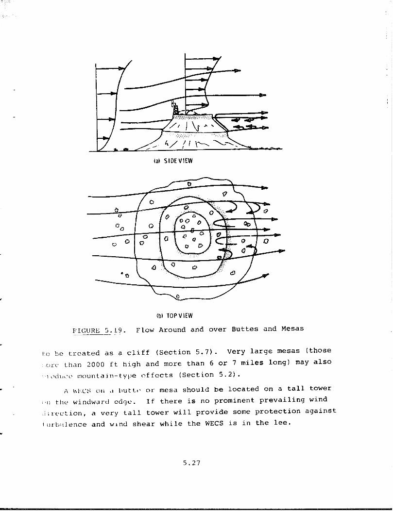
(al SIDE VIEW

(bl TOP VIEW

FIGURE 5.19. Flow Around and over Buttes and Mesas -___-

tto Se treated as a cliff (Section 5.7). Very large mesas (those

; (JLC than 2000 ft high and more than 6 or 7 miles long) may alSO

: 1 idll~-t., mountain-type c!ffects (Section 5.2j.

tl \%l~:c.'; 011 -1 t>uttc> or mesa should be located on a tall tower

1.11 the windwarcj edge. If there is no prominent prevailing wind

:ik-~~tion, '. . a very tall tower will provide some protection against

!ilr-bi!lence and wind shear while the WECS is in the lee.

5.27

Y

5.9 ECOLOGICAL INDICATORS OF SITE SUITABILITY

Vegetatior‘. deformed by high average winds

estimate the average speed (thus power) and to

can be used both to

compare candidate

sites. This technique works best in three regions: 1) along

coasts, 2) in river valleys and gorges exhibiting strong channel-

ing of the wind, and 3) in mountainous terrain. Ecological indi- cators are especially useful in remote mountainous terrain not

only because there are little w.:nd data, but because the winds are

often hiqhly variable over small areas and difficult to character-

ize. The most easily observed deformities of trees (illustrated

in Figure 5.20) are listed and defined below:

0 Brushing-- Branches and twigs bend downwind like the hair of

a pelt s:lhich has been brushed in one direction only. This

deformity can be observed in deciduous trees after their

leaves have fallen. It is the most sensitive indicator of

light winds.

0 Flagging--Branches stream downwind, and the upwind branches

are short or have been stripped away.

0 Throwing --A tree is windthrown when the main trunk and the

branches lean away from the prevailing wind.

0 Clipping--Because _ strong winds prevent the leader branches

from extending up to their normal height, the tree tops are

held to an abnormally low level.

0 Carpeting--This deformity occurs because the winds are so

strong that every twig reaching more than several inches above

the ground is killed, allowing the carpet to extend far downwi nd .

F 1 ,!Ul‘C> 7s .?I) 1s one of the best guides to ranking tree deform- : t I C','. IJ->. wind sk"‘l>d. Both 3 top view and a side view of the tree Ii f' sllc~wr~ to cil~ntonstr'ate the brushing of individual twigs and

5.28

PREVAILING WIND

=

kYRONG FLAGG I NG

V CLIPPING AND FL&GING

VI R

VII THROWING EXTREME AND FLAGG I NG

@??cfzr

FLAGG I NG

FIGURE 5.20. Wind Speed Rating Scale Based on the -- Shape of the Crown and Degree Twigs, Branches, and Trunk are Bent (Griggs-Putnam Index)(lT)

branches and the shape of the tree trunk and crown. The figure

uses the Griggs-Putnam classification of tree deformities described

by indices from 0 to VII. When WECS sites are ranked by this

scheme, ol?l 1 should be compared, because

IilTf~~l~~nt types c>f trees may not be deformed to the same degree.

i\r~ot.h~~r .locxi indicat.or of relative wind speeds is the defor- I~i,~t-ioll rdt io. (17) It also measures how much the tree crown has 1N’C~II f laqqcd . Figure 5.21 shows the two angles, a and b, that

5.29

PREVAILING

WIND

D I RECT ION

FIGURE 5.21.

d

*

c

must be measured to compute the deformation ratio “D”. To measure these angles, the trees can either be photographed or sketched to

scale. (The user might sketch the tree on clear acetate while he

loc>ks at it through the acetate.) He should draw or take the tree

p.Yctures while viewing the tree perpendicular to the prevailing

wind direction so that he can see the full effects of flagging.

USE ONLY THE UPPER l/3 OF THE TREE FOR THIS MEASUREMENT

Deformation Ratio Computed as a Measure of the Degree of Flaqqinq(l~)

To compute D, the two angles shown in the figure (a on the

downwind side and L on the upwind side) should be measured in

degrees using a protractor and then divided (D = a .: b). The

larger the value of D, the stronger the average wind speed.

Nean annual wind speed is correlated with the Griqqs-Putnam

Index (Fiqure 5.20) in Table 5.3, and with the Deformation Patic (P'igurc 5.21) in T~blc 5.4. These reflect only preliminary research

results based on studies of two species of conifers, the Douglas Fir aI;d t hc Ponderosa Pine. Further studies are examining these and c:thcr tree species to improve predictions of mean annual winds with ~~~~~~l~~~ ica i ind ic;it.ors.

TABLE 5.3. Mean Annual Wind Speed Versus the Griqqs-Puttnam Index(a)

Griqqs-Putnam Index (as in Figure 5.20) I II III IV V - - - -

Probable Mean Annual Wind Speed Range (mph) 6-10 8-12 11-15 12-19 13-22

(a) These data were prepared by E. W. Hewson, J. E. Wade, and R. W. Baker of Oregon State University.

TAELE 5.4. Mean Annual Wind Speed Versus the Deformation Ratioia)

Deformation Ratio (as in Figure 5.21) I II III IV v VI VII -- - -

Probable Mean Annual Wind Speed Range (mph) 4-8 7-10 10-12 12-15 14-18 15-21 16-24

(a) These data were prepared by E. W. Hewson, J. E. wade, and R. W. Baker of Oregon State University.

Because they are based upon limited data, Tables 5.3 and 5.4

should only be used to locate possible areas of high wind energy

and to select candidate sites within such areas. The user should

not select a particular WECS based on ecological indicators alone.

A wind measurement proqram is recommended before the type of WECS

and final site are selected.

Table 5.5 gives the results of some early attempts (about 1948)

to estimate average annual wind speeds based on the Grigqs-Putnam

indcs for certain everqrcens in the Northeast. Though different

:;~'eci(:s are often deformed to different extents by the same winds,

ver1' strong winds (those capable of causing strong flagging, clip-

i:inq , or carpeti.nq) affect different species the same. Comparison

c)f the d:tta presented in Table 5.3 (based on Douglas Fir and

i’onderosa Pine) and Table 5.5 (based primarily on Balsam) bears

cut this fact.

5.31

TABLE 5.5. Griggs-Putnam Index Versus Average Annual Wind Speed for Conifers in the Northeastern United States (Adapted from Reference 18, Power from the Ws by Palmer Cosslett Putnam, 01975 by Allis Chalmers Corporation. Reprinted by permission of Van Nostrand Reinhold Company, a Division of Litton Educational Publishing, Inc.)

T\*~es of DcformatiOn Tree Height Velocity at Tree (Gt-iLqs-Putnam Indes) Description (Feet) Heigh_!t_ (mph) ____.. . --_- --

c‘.lt-p*t incl I3alsam, sl)rucc 1 27.0 (VlIl) ‘111ti f i I- held to

1 ft Clipping (V,

Balsam, spruce 4 21.5 and fir held to 4 it

Throwing (VI) f'laqqing (IV)

Ralsam thrown

Balsam StrOngly

flagged

25 19.2

30 18.6

Fldgging Balsam moder- (111) ately flagged

30 17.9

Flagging Balsam mini- (III mally flagged

40 17.3

Bt-ushiny Balsam not ( I i flagged

40 15.5

Flaqqinq (II)

ticmlcck and white pint she-d minima!. f laqqiny

40 lo.6

Though the presence of one type of deformity (or a combina-

tion) may indicate an area of high average winds, and the degree

of deformity may give estimates of the relative strengths of the

Wl nrls, there are still pitfalls to rating sites according to tree

deformity. Because past or present growing cond.itions can greatly

affect the size and shape of trees, only isolated trees appearing

to have grown under similar conditions should be compared. For cs.l:npl t', a tree in or near a dense stand of timber shouid not be Cc)mj2al-c>il to an isolated tree. Another fact to be aware of is that

limbs are stripped from trees not only by strong flagging. They c.13 be ci,lmayed b;, man, disease, other trees that once grew nearby,

5.32

or possibly ice storms. Misinterpreting such signs could lead to

the wrong assumptions about the prevailing wind direction and the

average speed. Common sense, however, should reveal whether or

not all the deformities observed in an area fit together into a B

consistent pattern.

The following guidelines summarize this section and suggest

how to use ecological indicators effectively:

1) detect ecological indicators of strong wind;

2) compare isolated trees within the strong wind areas to select

candidate sites;

consider flow patterns over barriers, terrain features, and

surface roughness in the final selection:

measure the wind to insure that the best site in complex

terrain is selected: and

base selection of a particular WECS and estimation of its

power output on wind measurements, not on ecological indi-

cators alone.

5.33

6.0 METHODS OF SITE ANALYSIS

Winds at a particular site may be recorded and analyzed by

any one of three methods described in Table 6.1. Once the winds

are recorded, the expected power output of a WECS may be computed.

The first method is the same one suggested in the preliminary

feasibility study (page 1.2). It requires only a knowledge of the

average annual wind speed, which can be obtained for nearby sta-

tions. Appendix A lists sources of wind climatology.

With this method, how frequently wind speeds occur is assumed

to del'end only on the mean wind speed. This allows computation

of tl-.c out})ut power from the mean annual wind speed and the WECS's

operating characteristics (i.e., cut-in, rated, and cut-out wind

speeds). However, care must be exercised in assuming that the

mean wind at the site is about the same as that at a nearby weather

station. That assumption may be true if both locations are within

a few miles of each other and if both are in the same large area

of flat ;lerrain (e.g., the Great Plains, a large plateau, or a

large basin).

The second method is more accurate than the first. An odometer-

t)'lx wind recorder, which measures the miles of wind passing by the

51t.e itIlt: wind run) , should be used for a minimum of three months

1.0 ctlllect onsitc? data, preferably during the three most windy

fi?OIltfl~j . A simple? method of correlating wind and computing output

iJower is presented in Appendix D.

The third method Is the only reliable one for estimating

:CWCI- CjUtpUt in complex terrain. Mountains, valleys, and other

f.cypo(:ra;-,t;ical features cause the wind to vary from one location tc‘ 31~(~thCt-, and )idst attempts to correlate such winds have not : (“‘1, 'Q1l, -t .'i:,: i, I . :';II c‘lit i 1-c year of data should be r:olle,:ted at

~'.lIICI I (!<I 11' s I I<‘!< I II ~.'l)!i\l‘i ('1. tci-rain.

0 . 1

__

.

TABLE 6.1. Various Approaches to Site Analysis

Method Approach

1 Use only mean annual speed from a nearby station: determine annual power output (using Appendix C).

2 More accurate than first method. Works well in all but very hi 1 ly or mountainous terrain.

Make 1 imi ted onsi to wind measurements, c.stablish rouqh cor- rc*lat ion with nearby station, then com- IJute power outpllt (usinq Appcndlx I)).

cc>i lcct wind data for tto site and analyze It to obtain annual power output (using methods in Appendix DJ .

Most accurate method. Works in all types of terrain.

Advantages

Little time or ex- pense required for collecting and analyz- ing data. If used properly, can be highly accurate.

Disadvantages -- Only works well in large area of flat terrain where average annual wind speeds are 10 mph or greater.

Requires time to collect data. Data period must represent typical wind conditions. Added cost of wind recorders. Works poorly in mountains.

Requires a year of data collection. Added costs of wind recorders. Data period must represent typical wind conditions.

Simple odometer-type devices can be purchased for about $100

or can possibly be rented from WECS dealers. By recording the

miles of wind monthly and dividing miles by the number of hours

in the month, the monthly average wind speeds (and in the same

manner the anni;al average wind speed) can be computed. With that

data anti Appendix C, average output power can be estimated.

T11ca wind recorrfina equipment used will dictate how the data

> .z ; . dllalyzed. An odometer-type recorder is the least expensive,

but iJro.Jidcs no wind direction information. More sophisticated

re:.ordinG equipment is available which can gather the type of data

cant aincd in the wind summaries described in Appendix D, as -well

as other useful wind information. Some of this sophisticated

C‘ L: Ii 1 Ume i i t costs under $1000, but can possibly be rented from WECS

dlstrlbntors. Since this ecjuipment will sort winds by both direc- t :(“l a:11i s { )CCCl , ' it will provide a more accurate estimate of out&ut ;‘(Jhl'! , tt w~l! better- tinable the user to select the most suitable WI, C. , and : t ~:ay also cnabi? him to select a site less affected by ii :f . :et c is2c CB.U~;I) lr in Section 4.3.3 and use of wind summaries i " . ; :‘t I‘ .- : : :'.. !

Those wishing to perform their own analysis may contact the

American Wind Energy Association (AWEA) for lists of manufacturers

. who produce various types of wind-measuring devices and accessories

(see Section 1 for the address). If such equipment is bought or

rented, it should be located according to the same guidelines sug-

gested in this handbook for an actual WECS.

The rcadcr might also consult the following reference on wind

measurement:

Snertcch Corporation Planning a Wind-Powered Generating System -- Box 420 Norwich, Vermont 05055.

Another method of collecting onsite data might be considered.

Some WECS dealers have equipment which can be programmed to simu-

late the power output of a particular WECS. This method permits

direct readout of power output for one type of WECS, but decreases

the ability to select the best WECS for the site.

If the user prefers, WECS dealers and meteorological consul-

tants can be employed to analyze a site. The AWEA can furnish the

names of some firms which provide such a service.

tihcn the sit<, analysis is completed and the final choice of

.I WCS is made, the: usc!r should remember that the operating char-

Jcteristics of the most suitable WECS for a particular site will - depend on his power needs and the wind characteristics at the - c: +e. -&c The need for a backup or energy storage system will depend

on the maximum expected return time of the wind (MERT). MERT is

t he longest interval in which the wind might remain below the WECS

-kit-in speed (i.e., the longest period in which no power will be

17.3tti 011 blt'K1' is s\vailable for some weather stations, but, if

.: ic; not available for a nearby station, it can be estimated dur- i IlCj t-hc! data co1 lecti<jn process. If sophisticated wind recorders

6.3

are used, they can probably be programmed to determine return times

automatically. If simple wind odometers are used, they must be

read at least once or twice daily during low wind periods to esti-

-.

mate the MERT. Though maximum return times often occur in autumn,

it is best to examine an entire year of data to estimate the return

time.

.

- *

S.-i

7.0 REFERENCES

1 -.

2.

3.

4.

5.

6.

7.

a.

(1 .

i0.

Survey of Historicai and Current Site Selection Techniques for the Placement of Small Wind Energy Conversion Systems. Report to Battelle, Pacific Northwest Laboratories by American Wind Energy Association, Bristol, IN 46507, February 1977.

J. Park and D. Schwind, Wind Power for Farms, Homes, and Small Industry. Prepared for the Energy Research and Development Administration by Nielsen Enqineering and Research, Inc., Mountain View, CA 94043 (in-press, scheduled for publication in June 1978).

II . c . s . Thorn , "New 1)istributions of Extreme Winds in the United Statcsi" Journal of the Structual Division, Proceedings of the Amer. Sec.-of Civil Eng. 94(ST7):1787-1801, July 1978. - - -

The National Atlas of the United States of America. Compiled by the U-S ;.ept. of Interior, Geological Survey, Washington, DC, 1970.

M. E. Pautz, Severe Local Storm Occurrences, 1955-1967. ESSA Technical Memorandum, WBTM FCST 12, reprinted by and available from iu’&Qi, Siiver Spring, MD 209i0, May 1974.

John D. Stevenson, "Application of Tornado Technoiogy to Nuclear Industry." Proceedings of the Symposium on Tornadoes, Assessment of Knowledge and Implications for Man, June 22-24, 1976, Institute for Disaster Research, Texas Tech University, 1‘ . 0 . Box 4089, Lubbock, TX 79409.

I ven Bcllnct , Gldzc: : Its Meteorology and Climatology, Gcograph- 7----- -.-I_ ical Distribution. and Economic Effect. EF-105, QuartermastY?r,

Technical Report Research and Engineering Center,

Natick, MA, March 1959.

T (I. I-* . Daniels, ed., Terrestrial Environment (Climatic) Cri- tcria Guidelines for Use in Space Vehicle Development. NASA- -- __------ 'i'M-X-645891 Marshall Space Flight Center, AL, I.971 (revised).

?1 . ?i . c)rlli 11 .lntl !:. A. Sehmel, "Frequency and Diurnal Varia- tion of Dust Storms ii1 the Cont.iguous U.S.A." Atmos. Environ. 10(10):813-825, 1376.

I?: . Pros,t and II). Nowak, flandbook of Wind Turbine Generator Siting Techniques Relative to%xensional Terrain Features. -- fiepared f(lTl'-battello, Pacific Northwest Laboratories by FWG f%sociatcs, Inc., Tullahoma, TN 37388, November 1977.

7.1

11.

12.

13.

14.

15.

16.

17.

18.

1. 9 .

20.

21.

LL!.

V. A. Sandborn, Placement of Wind-Power Systems. EY-76-S-06- 2438, Colorado State University, Fort Collins, CO, 1977.

J. Van Eimern, R. Karschon, L. A. Razumova, and G. W. Robertson, Windbreaks and Shelterbelts. Technical Note 59, World Meteor-

,

ological Organization, Geneva, Switzerland, 196'4.

R. N. Meroney, "Wind in the Perturbed Environment: Its Influ- - ence on WECS." Presented at American Wind Energy Association Conference, Boulder, Co, May 11-14, 1977, Colorado State Univ., Fort Collins, CO, 1977.

F. R. Eldridge, Wind Machines. NSF-RA-N-75-051, National Science Foundation Report prepared by Mitre Corp., available from U.S. Government Printing-Office; Washington, DC 20402, 1975.

J. Frenkeil, "Wind Profiles over Hills (in Relation to Wind- Power Utilization)." Quarterly Journal of the Royal Meteoro- logical Society 88(376):156-169, April 1962. -

F. Defant, "Local Winds," Compendium of Meteorology. T. F. Malone, ed., American Meteorology Society, Boston, MA, PP- 655-672, 1951.

E . A . I7 HeWSOn J . F. Wade , and R. W. Baker, Indicator of'High Wind Velocity.

Vxetation as an Prepared for the Energy

Research and Development Administration by Oregon State IJniversity: Corvallis, OR 97331, June 1977.

P. c. Putnam, Power from the Wind. Van Nostrand Reinhold Co., New York, NY, 1948, p. 84.

M. c:. Vcrhol c:h , Summar _ --.__ Sites.

y of Wind Data from Nuclear Power Plant ENWL-2220 WIND-I, Battelle, Pacific Northwest

Laboratories, Richland, WA 99352, 1977.

J . Reed, "Wind Power Climatology." Weatherwise 27(6):237-242, December 1974.

- --

D. L. Elliott, Synthesis of National Wind Energy Assessments. BXWL-2220 WIND-5, Battelle, Pacific Northwest Laboratories, Richland, WA 99352, 1977.

iv‘ . c . r'liff, 'J'hc Effect of Generalized Wind Characteristics on Annual Power Estimates from Wind Turbine Generators. -- PNL-2436, Biattelle, Pacificmhwest Laboratories, Richland, WA 99352, October 1977.

7 . 2

.

APPENDIX A

SOURCES AND USES OF WIND CLIMATOLOGY

SOURCES OF WIND CLIMATOLOGY

. The National Climatic Center (NCC! at Asheville, North

Carolina is usually the best source of wind data. NCC will, for

the cost of reproduction (usually a few cents per copy), provide

available summaries for sites in or near a locality. These data

may be obtained by writing to:

Director National Climatic Center Federal Building Asheville, North Carolina 28801

The wind summaries are generally similar to Table A.l. Frequently

wind roses have been constructed for stations. Figure A.1 illus-

trates a typical wind rose.

An index has been developed which lists all sites for which

wind summaries are available. These sites include past and present

National Weather Service Stations, Federal Aviation Administration

and Civil Aeronautics Administration sites, and military installa- L;^-^ Ll"‘,b. The index entitled index--Summarized Wind Data, by M. J.

Changery, W. T. Hodge, and J. V. Ramsdell, (BNWL-2220 WIND-ll),

September 1977, can be obtained from:

National Technical Information Service U.S. Department of Commerce 5285 Port Royal Road Springfield, Virginia 22151.

Wind climatology may also be obtained from utilities operat-

ing nuclear power plants. Reference 19 may also be helpful because

it contains summarized wind data from over 100 nuclear sites at the

locations shown in Figure A.2. The summaries include wind speed

I frcqucncies by direction, qraphs of wind speed versus duration of S~'CC?Cl , ht>irlht and lr~~ltion of the wind sensor, the average wind s[leed, the available wind power, and descriptions of the site and

. Chc surrounding terrain.

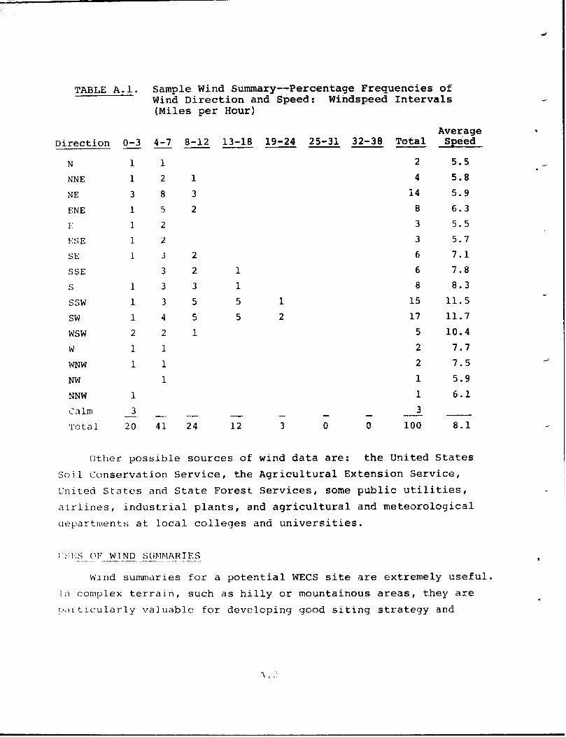
TABLE A.1.

Direction o-3 4-7 8-12

N NNE NE ENE F: I,:SE

SE SSE S ssw SW

wsw w

W-NW NW NNW Calm Total

1 1 3 1 1 1 1

1 1 1 2 1 1

1 3

1 2 8 5 2 2 3 3 3 3 4 2

1 1 1

20 41 24

Sample Wind Summary --Percentage Frequencies of Wind Direction and Speed: Windspeed Intervals (Miles per Hour)

13-18 19-24 25-31 32-38 Total c_L_--- 2 4

i4 8 3

1 1 5 1

5 2

3 6 6 8

15 17

5 2 2

1 1 3 - - -

12 3 0 0 100

Other possible sources of wind data are: the United States

Average Speed

5.5 5.8 5.9 6.3 5.5 5.7 7.1 7.8 8.3

11.5 11.7 10.4

7.7 7.5

5.9 6.1

8.1

Soil Conservation Service, the Agricultural Extension Service,

IJnited States and State Forest Services, some public utilities,

alrlines, industrial plants, and agricultural and meteorological

departments at local colleges and universities.

, TL. .,!,:5 OF WIND SLI~IMARIES ---

Wind summaries for a potential WECS site are extremely Useful. 711 complex terrain, such as hilly or mountainous areas, they are I:',\L'ticularly valuable for developing good siting strategy and

.

W

FIGURE A-1. Sample Wind Rose (constructed from Table A.l). Each arrow shaft is proportional in length to the percentage of time that the wind blows along the arrow. Numbers at the head of each arrow indicate the average wind speed for that direction.

estimating power output. Wind summaries from nearby weather sta-

tions can be used for flat terrain.

Wind roses (Figure A.l) show the percentage of time that the

wind blows from certain directions and the mean wind speed from

those directions. The user can construct a crude wind energy rose

from a wind summary table by first cubing the average wind speed

for each direction, then multiplying the cubed speeds by the per-

centage frequency of occurrence for each wind direction. An

example of this technique is given in Figure A.3, where Table A.1

has been used to construct the wind energy rose. The derived

numbers ;lre roughly proportional to the energy contained in winds

L)lowinli from eac'n direction.

A.3

.

.

SAMPLE CALCUATION: INTABLE A.lWIND FROIV\ THE NORTH BLOWS B(O.021 OFTHETIMEAND AVERAGES 5.5MPH.

5.5 x 5.5 x5.5x 0.02 = 3.3 (WHICH IS PLOllED ATTHEHEADOFTHEARROW SHAFTCOMINGFROMA NORTHERLYDIRECTIONI

W

N

21.5 - \ 272.3

f

7.8 ,: 2.3

S

E

I> LGuRl; A. 3. Smq)lc Wind Rncrrgy Rose (constructed .-- .-x- from Table A.11

c,

In Fiyure A.3 most of the wind power is associated with winds

blowing from the southwest, the prevailing power direction. The

tiser should determine the prevailing power direction for his siting

area and any other directions with which significant wind power is

associated. To minimize the adverse effects of barriers, he should

locate the> WT:CS so that there are no barriers upwind, along any of

.

A .5

.

APPENDIX B

INITIAL ESTIMATE OF WIND ENERGY POTENTIAL

IN~,~~I;L BST.TXATE OF WIND ENERGY POTENTIAL ----------

The best indicator of the practicality of WECS is the local history of WECS use. If WECS have been or are being used in the vicinity, users can supply useful information about the type, size, and application of their WECS; adequacy of the power output; sltiny procedures used; and accuracy of the estimated power output.

If there is no local history of WECS use, Figure B.1 provides ;r rot:cjh estimation of the wind power potential over the continental Ilnited States. In general, areas where available wind power is above 100 watts per square meter (wpsm) merit further investiga- t :. tin s Good WECS sites do exist in regions where available power is less than 100 wpsm, but are generally limited to small areas of T .,.ocallY enhanced winds, such as hills, mountains, ridges or sea-

CQaS ts l Figure B.2 illustrates this by presenting available power fcr only the higher elevations. The figure indicates that consid- erable wind energy is available even in the Southeast and the Southwest, which are shown as low power regions in Figure B.l.

Before deciding against using wind energy, the reader should examine the parts of Section 5 that discuss local landforms. But I.? the annual average wind speeds at nearby weather stations are less than 8 mph, and if there are no local terrain features to enhance the wind, small WECS are probably not practical.

B-l&'

I L-- ----- __.--. --- - ---.--_a .---.- -A.---

b ‘Z L

I R

I

/ Js / -

B.3

APPENDIX C

ESTIMATING POWFLR OUTPUT FROM ANNUAL AVERAGE WIND SPEEDS AND WECS CHARACTERISTICS

ESTIMATING POWER OUTPUT FROM ANNUAL AVERAGE WIND SPEEDS AND WECS CHARACTERISTICS

WECS CHARACTERISTICS NEEDED

cx = cut-In Speed = Wind speed below which the generator produces no electricity.

RS = Rated Speed = The lowest speed at which the generator produces power at its rated capacity.

CC? = Cut-Out Speed = The speed above which the generator does not operate (due to hazardous winds). If the machine does not cut-out, use a high speed (such as 50 mph).

PRK'EDURE TO ESTIMATE AVERAGE ANNUAL POWER OUTPUT -._._- __-. --

1.

7 L.

3.

4.

AA = Annual Average Wind Speed

The fcllowing relationships give the two required ratios:

co AA is-' RS

These two ratios are used in Figure C.l to determine

average power output rated power

This value multiplied by the rated power of the WECS gives the average power output (this will probably be in kilowatts).

Finally, the average power output in (in kW) multiplied by the i7 timber of hours per year (24 x 365 = 8760) gives the average ;I:lnual powr;r output (kW hours per year).

:-~m;igq I. ,*a- USEFili ESTIMATES L

'i'o estimate down time and running time:

I . Compute these two ratios:

CO CI Gi' AA

0.8

I '0 I 0.1 I 0.2 0.3 0.4 I 0.5 I 0.6 I 0.7 I 0.8 I 0.9 I 1.0 I 1.1 I 1.2 I 1.3 1 1.4 ! 1.5 I

’ ANNUAL MEAN WIND SPEED RATED WIND SPEED

CUT-OUT SPEED Rf!ED’ SPEEd

FIGURE C.l. Estimate of Expected Average Power Output for Wind Turbines.(22) (The dotted lines refer to the example given on Page C.4.)

2. These ratios were used in Figure C.2 to estimate the per- centage of the time the WECS will not be generating (100 - % down time = % running time).

To kstimate the percent of the time the WECS will be running at rated capacity:

1. Compute these ratios:

co Rs AA' AA -

\ . Estimate how much of the time the WECS will run at rated cal>acity from these ratios and the information in Figure C.3.

. . .

20

10

0 0 0.2 0.4 0.6 0.R 1.0 1.2 1.4

Cl11 IN VELOCITY ANNiJAL MiiItiVELOCIT?

FIGURE C.2. Percent Down Time. (22) (The dotted lines refer to the example given on Page C.4.)

c, 7

z 7 3 CY

?JY ---____ CUTOUT VELGCITY

\ \\\ 30

31

il 0. 2 0.4 0.h 0.8 1.0 1.2 1.4 1.6 + 1.8 2.0 RATtDVELOCITY

ANNUAL MEAN VELOCI iY 1.67

k'IGlIRE: C. 3. Percent Time Running at Rated. (22) (The dotted lines refer to the example given on Page C.4.)

c.3

Given:

Estimate:

/ EXAMPLE'PROBLEM

CI = 1.0 .mph RS = 2~0 fficiah

’

Rated Power = 5 kW

co = 40 w&l AA= 12 mph

1. Average annual power- output 2. Percent running tiine

1. 3. Percent time running at rated

co RS = 40 m 72 2.0 ii RS= 12 20= 0.60

Average power =

h

average power rated power x rated power = 0.34 x 5 kW - 1.7 kW

Annual power =

hours Average power x - = year 1.7 kW x 8760 hours = year

14892 kW hours -_- ----- _year-

2. co 40 -= m 12=3.33 CI 10 AA = 12 = 0.83

% down time = 45% .-I running time = 100% - 45% = 55% -

3. co - = -- 40 AA = 12 3.33 1.67

% running at rated = 10% .B

APPENDIX D

COMPUTATION OF OUTPUT POWER FROM WIND SUMMARIES

COMPUTATION OF OUTPUT POWER FROM WIND SUMMARIES

Two simple methods can be used to compute the output power from a WECS using a wind summary:

1) correlation of onsite data with nearby weather stations (see Method 2 presented in Section 61, and

;1 j computation of output power from a wind summary.

CuRRELATION OF WINDS WITH A NEARBY WEATHER STATION --

Select a nearby weather station located in the same type of terrain as the WECS site. (This technique does not work well in ritiu'ltainous terrain.) Collect wind speed data for at least three L*:ndy months of the year (late winter and spring are suggested) ,~nd use them to compute the average wind speed at the site for the period. Obtain the average wind speed at the weather station for this time period, as well as the long-term wind summary; then divjde the three-month average at the site by the three-month average at the station to get the correction factor. Using the !ony-term wind summary for the weather station, select the midpoint of each speed class and multiply it by the correction factor. In this manner a new wind summary can be constructed for the site wf!~ch uses the corrected midpoints of each speed class and the clriginal wind speed frequencies from the weather station summary. !.:;e the new wi.ld summary to compute power output.

t'~;AYF'LL CORRELATION PRQBLEM --~--

;:;veIi: 1: a three-month site average speed of 12.2 mph

-‘I a three-month weather station average speed of 10.1 mph L

3) the long-term wind summary from the weather station (use Table A.1 in Appendix A).

D. 1n

Construct a new wind summary (shown in Table D.l for the WECS

candidate site).

Midpoints of speed classes

0 - 3 = 1.5 13 - 18 = 15.5 4 - 7 = 5.5 19 - 24 = 21.5 8 - 12 = 10.0 25 - 31 = 27.5

4

?

r

4

Correction factor

Site 3-month average 12.2 Station 3-month average = m= 1.2

TABLE D.l. New Wind Summary

New Midpoints (old midpoints x 1.2) = 1.8 6.6 12.0 18.6 25.8 33.0 Old Frequencies of Wind Speeds (Table A.l) = 20 41 24 12 3 0

The next step would be to use the newly computed wind summary to compute output power according to guidelines in the following section of Appendix D.

COMPUTATION OF OUTPUT POWER FROM A WIND SUMMARY

The data needed are the output power graphs or tables for the WECS being considered (see Figure D.l) and a wind summary (provided in Table D-2). First, determine the midpoints of each speed class in the wind summary. (Speed classes entirely below the cut-in speed of the WECS need not be considered.) If the wind summary from a nearby weather station is used to compute output power directly (i.e., with no correlation), the midpoints of each speed class may need to be multiplied by a height correction factor. Tf the height of the wind sensor at the weather station is known, i I C‘.III bf* usctl <ts the base height. The correction factor can then I)#' cl(-! 1'1 111i ncvf 11:; I ncj tlic pl-oposed WECS height, Table 4.1, and the I list l‘lict i C’llS i II :;tv- t ion 4 . 1. (The user need not make the height

d

d

.-’

4

CUT-IN RATED CUT OUT

.- - --$----

,3.6-----t -- - I I

I I

2 I /I I I ;

a c -1.3 - .i -- a3 t-1 2 4 ’

i I 1 I I I

I I I I I I I I

19:o I

2+,5 I I

8.5 0 I I 1 I 37;u

0 5 10 15 20 25 30 35 40

WIND SPEED, MILES PER HOUR

FIGURE D-1. Hypothetical Output Power Curve

correction if the height of the wind sensor and the WECS height are within 10 ft of one another.) Using the power output graph or table for a particular WECS (such as Figure D.11, determine the output power for the midpoint of each speed class (Table D.3). Rc certain to convert all wind speeds to the same units before reading the output power. The final step is to multiply the out- put power for each speed class by the hours that the speed occurred (Table D.4); then add these products to obtain the total power expected per year.

Lsample of an Output Power Calculation from a Wind Summary -

Given: 1) the hypothetical power curve for a WECS in Figure D.l

2) the hypothetical percentage frequency of wind speed L and direction summary in Table 13.2.

~'~'lqnlt C' the> ti~~~~~uk~l power output of the WECS.

D.3

TABLE D.2. Hypoth+.c~&:Wind Summary (%'PreqUency of~~U+iP~eii~~)

E

ESE

SE SSE

S

ssw

SW

wsw

w

WNW

NW

NNW

CALM

% OF 'rime Winti 111 Spcxd ILIII~~"

0.1

0.4

0.4 0.3

0.4

0.4

0.7

0.6 0.9

0.4 0.5

0.3

0.6 0 . h

0.8

0.6

8.6 74.1 25.3 20.4 8.1

TABLE D.3. Hypothetical Output Power by Speed Class

z-. 2.0

1.2

1.3

0.7

0.1

0.8

1.5

1.7

2.1

1.6 1.5

0.9

1 . 6

1.7

2.5

2.2

2.3 1.7 0.6

1.4 1.3 0.4 1.4 0.6 0.2 0.4 Q.3 0.0

0.3 0.1 0.1 0.3 0.1 0.0 1.2 0.4 0.1 1.2 0.4 0.1 2.0 0.7 0.2 2.4 1.6 0.2

2.3 3.0 1.0

1.1 1.0 0.3 1.4 1.2 0.4

1.8 1.9 1.1

3.0 3.6 2.2

2.8 2.5 1.3

Midpoints of Speed Classes (mph) (Table D.2) Power at Midpoints (kW) from Figure D-1

0.0

0.0 0.0

0.1 0.0

0.4 0.1

0.1 0.0

0.6 0.1 100.0 8.8

Percbnt

: 7.5

4.7

3.9 1.7

1.7

1.7

3.9

4.0

5.9 6.3 8.3

3.6

5.3

7'. 6

14.0

10.0

9.8

Mean t+nd Speed

9.3

9.8 8.1 6.8

6.5

5.6 6.7

6.8

7.3 8.9

11.0

9.6

9.0

11.3

12.8

11.0

13.5 19.0 24.5 30.5 37.0

1.3 3.6 4.0 4.0 4.0

TABLE D.4. Conversion of % Frequencies to Hours Ihr/yr = 365 x 24 = 876-O)

Speed Class 13.5 19.0 24.5 30.5 37.0 Percent Frequency 20.4 8.1 3.0 0.6 0.1 Ilr ot. Occurrcncc/Yr (P x 8760 : 100) 1787 709 263 52 9

D.4

power at midpoint (kW) x hr of occurrence/yr = kW hr/yr.

1.3 x 1787 = 2323.1 3.6 x 709 = 2552.4 4.0 x 263 = 1052.0 4.0 x 52 = 208.0 4.0 x 9 = 36.0

Total kW hr/yr g171.5

If the user has collected and summarized a year of onsite winds, he should determine if the collected data is typical for the area. To do that wind statistics for the current year at a nearby station (i.e., the year in which onsite data were collected) can 1~ corn)>arctl with the lonq-term average at the station. All wind ~l)ecd c,bservations can bc corrected for an abnormal year by multi- plyinq them by this ratio: D/L, where "D" is the weather station annual average speed for the year of data, and "L" is the lonq- term average speed. For example, suppose the year examined was unusually windy. Assume that "L" for the nearest weather station was 10 mph, and "D" was 13 mph. To make the correction the mid- point of each speed class in Table D.3 should be multiplied by D/L, which equals lo/13 or 0.77. In this example multiplying by the ratio will reduce the power at the midpoints obtained from Fig- ure D.l. Completing the annual output power calculations will yield a lower, but more typical, annual power.

The output power computed above is the power flowing directly from the generator before any losses from resistance in the wiring or from an inefficient storage system. Such losses of power depend upon the system's design, and should be discussed with the dealer Lxforc a particular machine and storage/backup system is selected.

0.5

APPENDIX E

UNITS CONVERSION

UNITS CONVERSION

Length

Feet = Meters x 3.28 Meters = Feet x 0.305

Miles = Kilometers x 0.621 Kilometers = Miles x 1.609

Miles = Nautical miles x 1.15 Nautical Miles = Miles x' 0.869

Kilometers = Nautical miles x 1.852

Speed

Miles per hour (mph) = Meters per second x 2.24 Meters per second = mph x 0.447

mph = Knots x 1.15 Knots = mph x 0.869 Knots = Meters per second x 1.94

Meters per second = Knots x 0.514 Kilometers per hour = Meters per second x 3.6

Area

Square feet = Square meters x 10.76 Square meters = Square feet x 0.093

Power

Horsepower = Watts x 0.00134 Watts = Horsepower x 746

Horsepb-ver = Kilowatts x 1.34 Kilowatts = Horsepower x 0.746 Kilowatts = Watts x 1000

1,:. 13'