309-1

A Program for Robust Calculation of Drillhole Spacing in Three Dimensions

David F. Machuca Mory and Clayton V. Deutsch

Centre for Computational Geostatistics (CCG) Department of Civil & Environmental Engineering

University of Alberta

A robust algorithm and program to calculate the drillhole spacing in 3-D is developed. This program overcomes issues such as artefacts in regular grids, irregularity and over-smoothing of the resultant maps when a very small or very large constant search radius is used. Grade continuity and anisotropy are taken in account. Program performance is tested with synthetic and real data sets. The relation between geometric and probabilistic criteria is shown and used to define the limits for the resources categories.

Introduction

Different Resources and Reserves reporting codes highlight the data distribution/configuration as an important criterion to confirm the geological and/or grade continuity and thus, to classify the resources in Measured, Indicated and Inferred in order of decreasing geological confidence. These codes do not specify the thresholds for data spacing or other factors for mineral resource categories delimitation, giving a wide margin to the judgment and expertise of the Competent Person over the choice of the appropriate classification criteria.

Although the use of probabilistic criteria is not required by the resources and reserves reporting codes, they encourage the quantification of grade uncertainty. A purely probabilistic criterion of resources classification can be based in confidence intervals of the grade derived from the mean and standard deviation of simulated values scaled-up to SMU scale or production volumes in a certain period. These confidence intervals highly depend of the volume considered and have two components: the precision, expressed as an interval centered at the estimated grade, and the probability to be within this precision. The use of pure probabilistic criteria can be perceived as an objective and quantitative approach for resources classification, however they are affected by several issues (Deutsch, Leuangthong, Ortiz, 2006): Dependency of uncertainty in the modeling methods and parameters used, counter intuitive and non-transparent relation of the parameters with the uncertainty, the parameters uncertainty in itself, and the high sensitivity in the arbitrarily chosen probability thresholds, which can not be universal but very dependent of the deposit type.

Data spacing is very often directly related to grade uncertainty, it has been used traditionally as a determinant factor for resources classification, and it can be compared to the dimensions of relevant geological features for defining their continuity. Thus, a more complete criterion for mineral resources classification should be one that combines the geometrical features of data, as spacing and density, with different geological considerations, and is supported by probabilistic measures.

With the goal to implement these criteria a robust algorithm for local drill hole density and spacing mapping is needed. Spatial pattern point analysis has developed several methods for data density (intensity) calculation, such as kernel estimators (Cressie, 1994), which needs an

309-2

appropriate choice of the kernel bandwidth and smoothing function. However, a simpler methodology is developed here for meet the particular requirements of drilling for exploration and resources estimation. The main requirements are:

• The results must be smoothed enough to present a close to constant density and reproduce the nominal grid spacing for every point in areas where the drilling pattern regular.

• Over smoothing must be avoided in order to keep local precision and to detect areas where the grid spacing changes, i.e. from areas drilled for ore delimitation to sampling resources estimation.

• The algorithm must be easy to implement and use. The results must be easy to interpret and correlate to geological and operational aspects of drilling.

• The algorithm must be valid even when the drill holes are inclined or non parallel.

This algorithm developed and implemented in the Fortran program Spacing3D, reduces considerably the artefacts produced by the application of a constant area search window on a regular drill hole grid, provides a mean to control over smoothing or patchiness in the results, accounts for the anisotropy in grade continuity and can be used from regular to random 2D sampling and 3D drill hole arrays. When used in three dimensions, the program is not aimed to calculate the three dimensional data density, i.e. the number of data point per volume unit, but the equivalent bi-dimensional drillhole density and spacing.

Density and Spacing Calculation Criteria

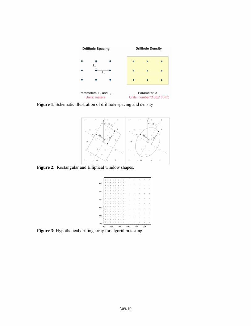
Sample density (or intensity, as it is called in spatial point pattern analysis) is defined as the number of data points per unit area. Sample or drillhole spacing has a particular definition for ore resources exploration where sampling and drilling is usually carried out in systematic regular patterns defined by a nominal grid spacing, particularly in the stages of delineation and sampling drilling. Thus, in this context, spacing can be defined as the average side length of the drilling mesh (see Figure 1).

In two dimensions, local sample density for a location u is calculated by the number of samples, ns(u), found within the limits of an anisotropic window of rectangular or ellipsoidal shape centered in u, (see figure 2) divided by the isotropic area A:

( )( ) 10000s unu

Aδ = × (1)

The sample density is expressed as the number of samples or drillholes per hectare. The initial dimensions and orientation of the search window are set in relation to the dimensions and orientation of the anisotropy ellipsoid, which is defined by the variogram model parameters.

When the search area has an elliptical shape, the isotropic area is calculated as the area of a circle with radius equivalent to the minor radius of the search ellipsoid:

( )2max hA sh aπ= ⋅ ⋅ (2)

Where shmax is the maximum horizontal search radius, and ah is the horizontal anisotropy factor defined as the quotient between the minimum and maximum horizontal anisotropy axis lengths,

minh and maxh , respectively:

309-3

min

maxh

ha

h= (3)

If a rectangular search area is used, the isotropic area is calculated as: 2

max(2 )hA sh a= ⋅ ⋅ (4)

The use of an anisotropic search area for counting the closest samples, but an isotropic area for density calculation, is meant to account for the anisotropic distances from the node to the surrounding samples.

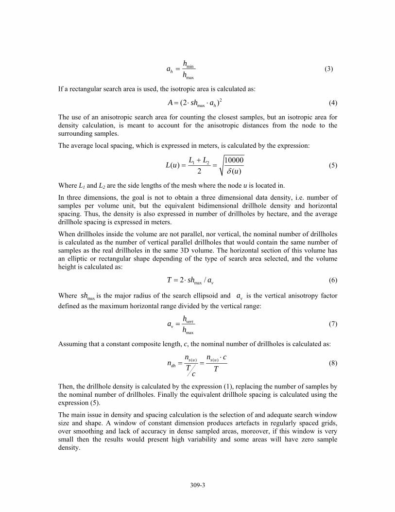
The average local spacing, which is expressed in meters, is calculated by the expression:

1 2 10000( )2 ( )

L LL u

uδ+

= = (5)

Where L1 and L2 are the side lengths of the mesh where the node u is located in.

In three dimensions, the goal is not to obtain a three dimensional data density, i.e. number of samples per volume unit, but the equivalent bidimensional drillhole density and horizontal spacing. Thus, the density is also expressed in number of drillholes by hectare, and the average drillhole spacing is expressed in meters.

When drillholes inside the volume are not parallel, nor vertical, the nominal number of drillholes is calculated as the number of vertical parallel drillholes that would contain the same number of samples as the real drillholes in the same 3D volume. The horizontal section of this volume has an elliptic or rectangular shape depending of the type of search area selected, and the volume height is calculated as:

max2 / vT sh a= ⋅ (6)

Where maxsh is the major radius of the search ellipsoid and va is the vertical anisotropy factor defined as the maximum horizontal range divided by the vertical range:

max

vertv

hah

= (7)

Assuming that a constant composite length, c, the nominal number of drillholes is calculated as:

( ) ( )s u s udh

n n cn T Tc

⋅= = (8)

Then, the drillhole density is calculated by the expression (1), replacing the number of samples by the nominal number of drillholes. Finally the equivalent drillhole spacing is calculated using the expression (5).

The main issue in density and spacing calculation is the selection of and adequate search window size and shape. A window of constant dimension produces artefacts in regularly spaced grids, over smoothing and lack of accuracy in dense sampled areas, moreover, if this window is very small then the results would present high variability and some areas will have zero sample density.

309-4

A methodology to overcome these drawbacks is described next. First the search window area A(d0,i) is defined as a function of the anisotropic distance d0,i between the node being estimated and the surrounding data points. Then the number of samples within the search area can be defined as the function:

0, 0,1

( ( )) ( , ( ))n

i j ij

N A d I u A d=

= ∑

Where n is the total number of samples in the data set, and ( , )j iI u d is an indicator variable of the form:

0,0,

0,

1 if ( )( , ( ))

0 if ( )j i

j ij i

u A dI u A d

u A d

∈⎧⎪= ⎨ ∉⎪⎩

Thus, the local density is calculated as:

max

min

0, 0,0

max min 0, 0,

( ( ) ) ( ( ))1 1( ) 100002 ( ) ( )

ni i

i n i i

N A d A N A du

n n A d A A dδ

=

⎛ ⎞− ∂= + ×⎜ ⎟⎜ ⎟− − ∂⎝ ⎠

∑

This expression can be understood as the mean of the average of density values before and after the search window area, A(d0,i), grows in a negligible area differential, A∂ , but enough to incorporate a new number of close samples within it. In the same way, the sample spacing can be calculated as:

max

min

0, 0,0

max min 0, 0,

( ) ( )1 1( ) 10000 100002 ( ( ) ) ( ( ))

ni i

i n i i

A d A A dL u

n n N A d A N A d=

⎛ ⎞− ∂= × + ×⎜ ⎟⎜ ⎟− − ∂⎝ ⎠

∑

The next section exposes the algorithm implemented in the spacing3d program; this is not only valid for sampling in two dimensions, as the last two expressions are, but also for the equivalent three-dimensional drillhole density and spacing calculation.

Implementation

In order to demonstrate and test the methodology introduced above, a hypothetical drilling pattern was designed. This is comprised of two regions: in the west side drillholes are located in a square grid of 40m spacing, and in the east side the spacing is 120m. Figure 3 shows this drilling array, a block model of 20m x 20m x 20m was superposed on it. For three selected sample blocks, located inside both grids and in the transition between them, the density and spacing was calculated using several sizes for the search window just before and after the limits of the search window grow enough to include a new sample or samples within it. For each one of the three sample blocks, figures 4a, 4b, 4c, 4d, 4e and 4f present these results as the relation of the anisotropic distances from the block to each surrounding sample versus the density and spacing calculated using such distance as the search window radius just before and after the sample falls within the search window area. For each new sample inclusion, the average of this pair of results is plotted as a continuous line in the graphs. As it can be observed in these graphs, neither density nor spacing are constants as the size of the search window changes, spacing grows until the search area grows without including new samples, then it drops abruptly. The inverse behaviour

309-5

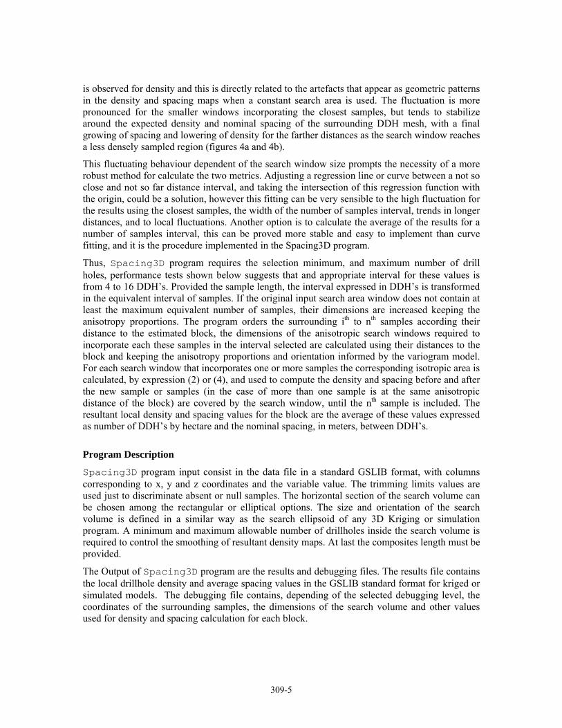
is observed for density and this is directly related to the artefacts that appear as geometric patterns in the density and spacing maps when a constant search area is used. The fluctuation is more pronounced for the smaller windows incorporating the closest samples, but tends to stabilize around the expected density and nominal spacing of the surrounding DDH mesh, with a final growing of spacing and lowering of density for the farther distances as the search window reaches a less densely sampled region (figures 4a and 4b).

This fluctuating behaviour dependent of the search window size prompts the necessity of a more robust method for calculate the two metrics. Adjusting a regression line or curve between a not so close and not so far distance interval, and taking the intersection of this regression function with the origin, could be a solution, however this fitting can be very sensible to the high fluctuation for the results using the closest samples, the width of the number of samples interval, trends in longer distances, and to local fluctuations. Another option is to calculate the average of the results for a number of samples interval, this can be proved more stable and easy to implement than curve fitting, and it is the procedure implemented in the Spacing3D program.

Thus, Spacing3D program requires the selection minimum, and maximum number of drill holes, performance tests shown below suggests that and appropriate interval for these values is from 4 to 16 DDH’s. Provided the sample length, the interval expressed in DDH’s is transformed in the equivalent interval of samples. If the original input search area window does not contain at least the maximum equivalent number of samples, their dimensions are increased keeping the anisotropy proportions. The program orders the surrounding ith to nth samples according their distance to the estimated block, the dimensions of the anisotropic search windows required to incorporate each these samples in the interval selected are calculated using their distances to the block and keeping the anisotropy proportions and orientation informed by the variogram model. For each search window that incorporates one or more samples the corresponding isotropic area is calculated, by expression (2) or (4), and used to compute the density and spacing before and after the new sample or samples (in the case of more than one sample is at the same anisotropic distance of the block) are covered by the search window, until the nth sample is included. The resultant local density and spacing values for the block are the average of these values expressed as number of DDH’s by hectare and the nominal spacing, in meters, between DDH’s.

Program Description

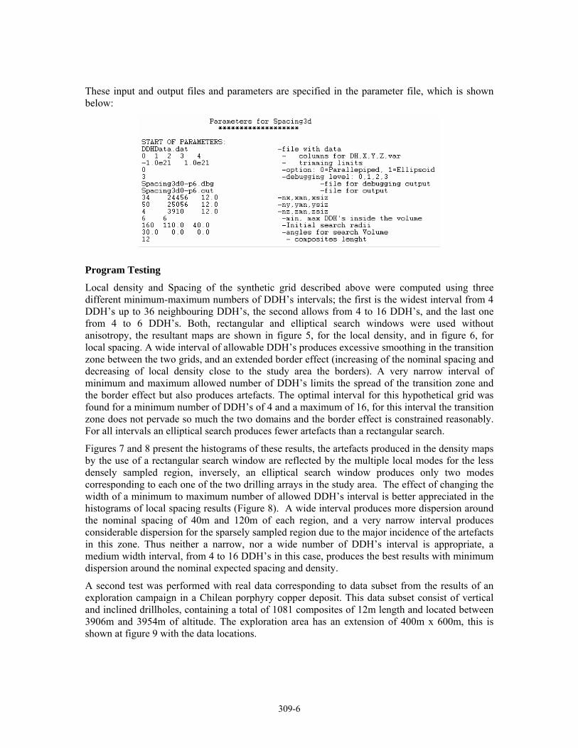
Spacing3D program input consist in the data file in a standard GSLIB format, with columns corresponding to x, y and z coordinates and the variable value. The trimming limits values are used just to discriminate absent or null samples. The horizontal section of the search volume can be chosen among the rectangular or elliptical options. The size and orientation of the search volume is defined in a similar way as the search ellipsoid of any 3D Kriging or simulation program. A minimum and maximum allowable number of drillholes inside the search volume is required to control the smoothing of resultant density maps. At last the composites length must be provided.

The Output of Spacing3D program are the results and debugging files. The results file contains the local drillhole density and average spacing values in the GSLIB standard format for kriged or simulated models. The debugging file contains, depending of the selected debugging level, the coordinates of the surrounding samples, the dimensions of the search volume and other values used for density and spacing calculation for each block.

309-6

These input and output files and parameters are specified in the parameter file, which is shown below:

Program Testing

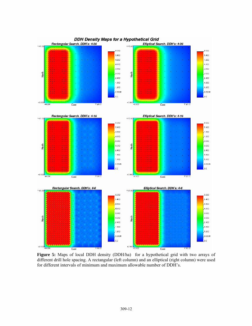
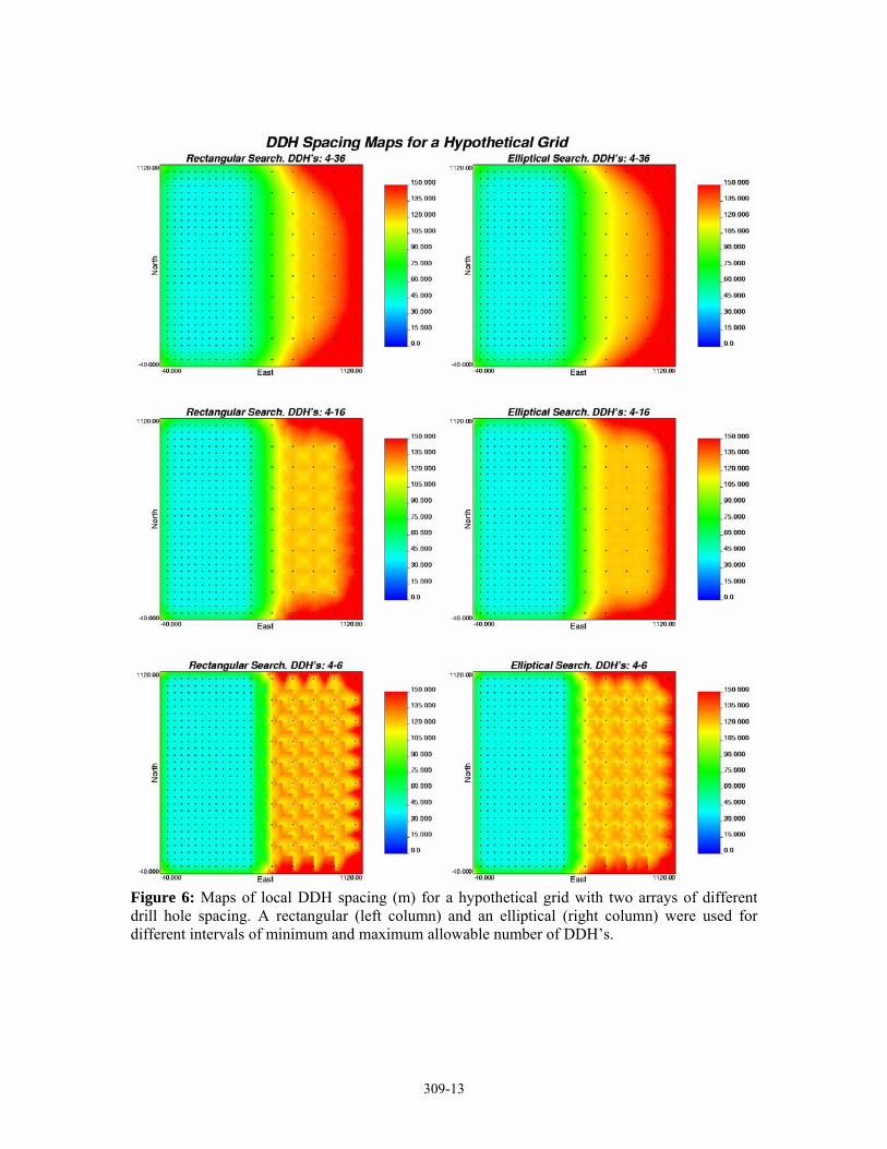
Local density and Spacing of the synthetic grid described above were computed using three different minimum-maximum numbers of DDH’s intervals; the first is the widest interval from 4 DDH’s up to 36 neighbouring DDH’s, the second allows from 4 to 16 DDH’s, and the last one from 4 to 6 DDH’s. Both, rectangular and elliptical search windows were used without anisotropy, the resultant maps are shown in figure 5, for the local density, and in figure 6, for local spacing. A wide interval of allowable DDH’s produces excessive smoothing in the transition zone between the two grids, and an extended border effect (increasing of the nominal spacing and decreasing of local density close to the study area the borders). A very narrow interval of minimum and maximum allowed number of DDH’s limits the spread of the transition zone and the border effect but also produces artefacts. The optimal interval for this hypothetical grid was found for a minimum number of DDH’s of 4 and a maximum of 16, for this interval the transition zone does not pervade so much the two domains and the border effect is constrained reasonably. For all intervals an elliptical search produces fewer artefacts than a rectangular search.

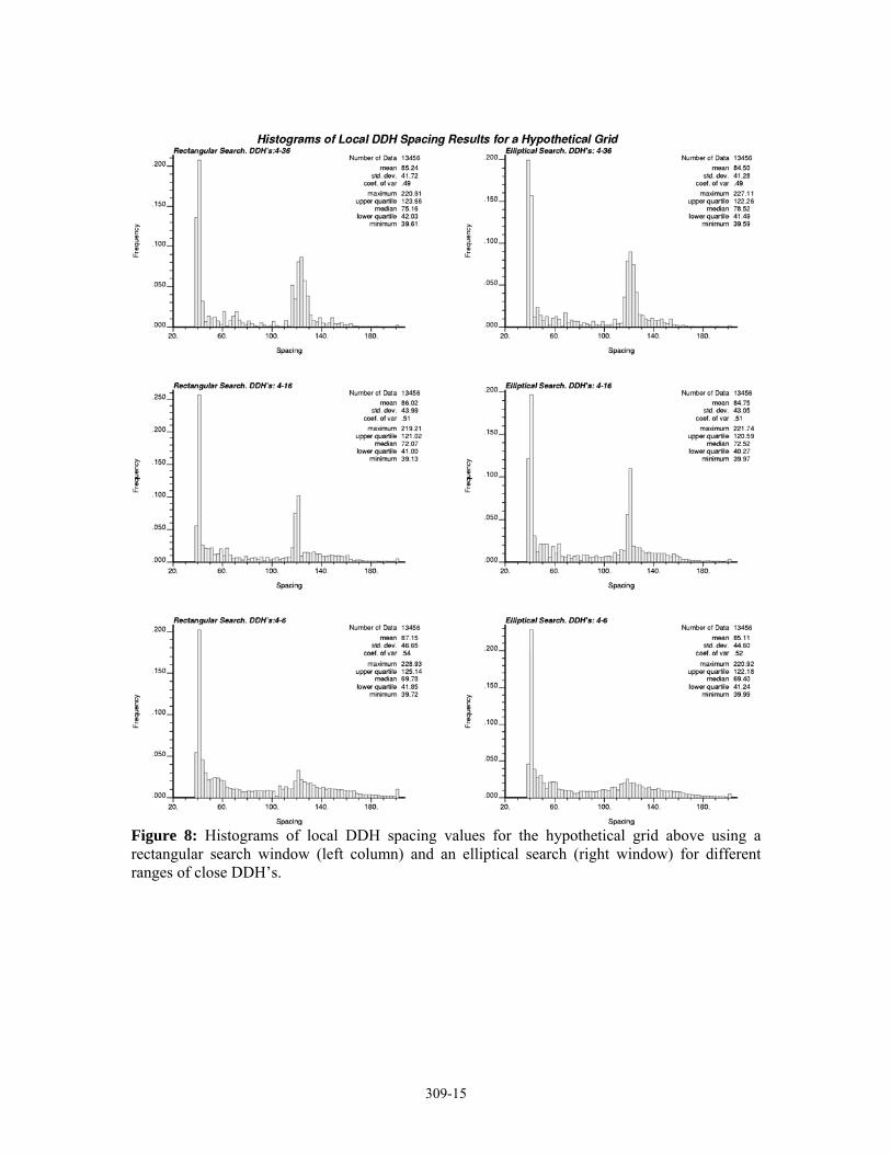
Figures 7 and 8 present the histograms of these results, the artefacts produced in the density maps by the use of a rectangular search window are reflected by the multiple local modes for the less densely sampled region, inversely, an elliptical search window produces only two modes corresponding to each one of the two drilling arrays in the study area. The effect of changing the width of a minimum to maximum number of allowed DDH’s interval is better appreciated in the histograms of local spacing results (Figure 8). A wide interval produces more dispersion around the nominal spacing of 40m and 120m of each region, and a very narrow interval produces considerable dispersion for the sparsely sampled region due to the major incidence of the artefacts in this zone. Thus neither a narrow, nor a wide number of DDH’s interval is appropriate, a medium width interval, from 4 to 16 DDH’s in this case, produces the best results with minimum dispersion around the nominal expected spacing and density.

A second test was performed with real data corresponding to data subset from the results of an exploration campaign in a Chilean porphyry copper deposit. This data subset consist of vertical and inclined drillholes, containing a total of 1081 composites of 12m length and located between 3906m and 3954m of altitude. The exploration area has an extension of 400m x 600m, this is shown at figure 9 with the data locations.

309-7

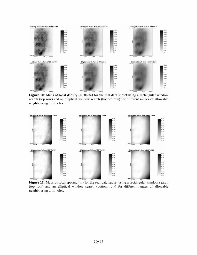
The Spacing3D program was executed using this data in a 408m x 600m x 48m volume discretized in a 12m x 12m x 12m three-dimensional mesh. An example of the resultant maps of local density and drillhole spacing are shown in figures 10 and 11. The rectangular and elliptical search options were tried for different selections of minimum and maximum allowed number of drillholes. The results show clearly the consequences of changing the search area shape and the allowed number of drillholes.

The dimensions and orientation of the search area were defined from the spatial continuity analysis, thus the major horizontal axis is 160m with 30° of azimuth, and the minor horizontal axis and the vertical axis lengths are 110m and 40m, respectively. The plunge and dip of the search area were set as 0.

The same effect of changing the interval width of allowed number of DDH’s observed for the synthetic grid is observer for the this real data subset, this is, scattered maps and presence of artefacts related to sampling pattern for narrow intervals, and over smoothing in the maps created using a very wide interval.

Relation between geometric and probabilistic criteria for resources classification

In basis of geological observations and the results of grade variability analysis, a geologist can determine for each domain in the deposit the sampling or DDH spacing that define the limits of measured / indicated and indicated / inferred resources. These limits usually are lower that the maximum variogram range, since the uncertainty of estimates can grow very quickly as the samples distance to the estimated block increases, even if this distance is lower than the variogram range. Moreover geological features as spacing of mineralized structures, geological controls, and others may complement the variogram analysis to define the appropriate spacing thresholds for resource classification. In order to illustrate the geometric criteria of resources classification, it has been supposed that, for the real data subset described above, the geological and grade continuity can be confirmed within 24m, therefore, in concordance with the Resources Reporting Codes, measured resources can be enclosed within the zones where DDH spacing does not exceeds this distance. In the same way, it could be stated that for areas where DDH spacing exceeds 48m, the geological and grade continuity can only be assumed but not verified, then the inferred resources are located in the areas where spacing is greater than this length.

By the other side, a pure probabilistic criterion was applied to the results of 100 realizations generated by Sequential Gaussian Simulation with a variogram of major anisotropy axis of 160 meters, 30º of azimuth and an anisotropy ratio of 1.45. The resources where classified as measured, indicated and inferred using probabilistic confidence intervals on the mean and standard deviation of the simulated values of each block. The limit between measured and indicated resources was defined for a precision of 20% with a confidence value of 75%, and the limit between indicated and inferred resources, for a precision of 45% with the same confidence. These values can be transformed to coefficient of variation (CV) values, thus, the first limit expressed as the CV becomes 0.289 and the second 0.406.

The resources classification maps using both criteria are shown in figure 13 and the scatter plots of the CV vs. local density and CV vs. local spacing are presented in figures 14 and 15. As expected, the CV and local density approaches to an inverse hyperbolic relationship, while the relationship between the CV and the local DDH spacing is direct. The moderate correlation coefficients reflect the fact that the probabilistic criterion can classify as measured resources

309-8

blocks in areas where the local DDH density is very low, and the presence of more than one population of blocks with high CV in relation to the local DDH spacing.

If the geometric criterion is taken as the principal resources classification criteria, a combined geometric and probabilistic criterion can be summarised, for this particular case, in the next table:

Table 1: Equivalence between parameters of Geometric Resources Classification Criteria and Probabilistic Criteria

Coefficient of Variation

Precision Value at 75% confidence Resource

Category DDH Spacing DDH Density Min. Mean Max Min. Mean Max Measured ≤ 24 ≤ 17.36 0.102 0.184 0.289 11.7% 21.2% 33.2% Indicated > 24, ≤ 48 > 17.36, ≤ 4.34 0.097 0.218 0.406 11.2% 25.1% 46.7%

Inferred > 48 > 4.34 0.133 0.298 0.543 15.2% 34.3% 62.5%

Discussion and Conclusions

Drillhole spacing calculation is dependent of the search window area used. A fixed window size leads to certain geometric artefacts. Smoothed maps are required, but excessive smoothing cause imprecise maps and removal of local details. The algorithm developed and implemented in the Spacing3D program reduces the artefacts and controls smoothing. For each location, the calculation results for a series of window sizes required to include each drillhole within an interval of minimum to maximum number of surrounding drillholes. A narrow interval produces artefacts; a wider one can smooth the results so much. The orientation and proportions of the search window are defined by the variogram anisotropy orientation and ratios. The algorithm allows the use of rectangular or elliptical search window section; elliptical work better. Once the appropriate interval of minimum and maximum number of drillholes is found (the tests show that best results can be obtained with a interval of around 4 to 16) the resultant density and spacing maps are smoothed enough to delimit continuous regions for each resource category, consistent with local information density and without the category rings around the drill holes that often pure probabilistic and other methods of resources classification present.

Classification criteria based primarily on information availability and spacing can be more directly and intuitively linked to geological features of the deposit than probabilistic criteria. In general, data density and the values of probabilistic measures of estimation uncertainty are related. It is recommended that the geometric criteria of classification be supported with estimation accuracy measures such as confidence intervals or coefficients of variation calculated from the mean and standard deviation of several simulated realizations.

References Cressie, N.A.C., 1991. Statistics for Spatial Data. Wiley-Interscience, New York.

Deutsch, C.V., Leuangthong O. Ortiz C, J. 2006. A Case for Geometric Criteria in Resources and Reserves Classification. CCG Meeting 2006. Centre for Computational Geostatistics (CCG), University of Alberta.

Deutsch, C.V. and Journel, A.G., 1998. GSLIB: Geostatistical Software Library: and User’s Guide. Oxford University Press, New York, 2nd Ed.

309-9

The Joint Ore Reserves Comitee of The Australasian Institute of Mining and Metallurgy, Australasian Institute of Geoscientists and Minerals Council of Australia (JORC), 2004. Australasian Code for Reporting of Exploration Results, Mineral Resources and Ore Reserves. The JORC Code.2004 Ed.

Snowden, D. V., 2001, Practical interpretation of mineral resource and ore reserve classification guidelines, in Edwards, A. C., ed., Mineral Resource and Ore Reserve Estimation – The AusIMM Guide to Good Practice: The Australasian Institute of Mining and Metallurgy, Monograph 23, Melbourne, p. 643-652.

309-10

Figure 1: Schematic illustration of drillhole spacing and density

Figure 2: Rectangular and Elliptical window shapes.

Figure 3: Hypothetical drilling array for algorithm testing.

309-11

F ig. 4b: Spacing values vs. search windo w radius

B lo ck co o rdinates: (245,545) . 40m x 40m grid zo ne.

3032343638404244464850

0 50 100 150 200 250 300 350 400

R adius ( m)

spacing (r-dr)spacing (r+dr)Average spacing

F ig. 4d: Spacing values vs. search windo w radius

B lo ck co o rdinates: (545,545) . T ransit io n zo ne.

50

60

70

80

90

100

110

120

130

0 50 100 150 200 250 300 350 400

R ad ius ( m)

spacing (r-dr)spacing (r+dr)Average spacing

F ig. 4a: D ensity values vs. search windo w radius

B lo ck co o rdinates: (245,545) . 40m x 40m grid zo ne.

4.00

5.00

6.00

7.00

8.00

9.00

10.00

0 50 100 150 200 250 300 350 400

R ad ius ( m)

density (r-dr)density (r+dr)Average density

F ig. 4c: D ensity values vs. search windo w radius

B lo ck co o rdinates: (545,545) . T ransit io n zo ne.

0.00

0.50

1.00

1.50

2.00

2.50

3.00

3.50

0 50 100 150 200 250 300 350 400

R ad ius ( m)

density (r-dr)density (r+dr)Average density

F ig. 4e: D ensity values vs. search windo w radius

B lo ck co o rdinates: (845,545) . 120m x 120m grid zo ne.

0.20

0.40

0.60

0.80

1.00

1.20

1.40

1.60

0 50 100 150 200 250 300 350 400

R ad ius ( m)

density (r-dr)density (r+dr)Average density

F ig. 4f : Spacing change vs. search windo w radius

B lo ck co o rdinates: (845,545) . 120m x 120m grid zo ne.

8090

100110120130140150160170

0 50 100 150 200 250 300 350 400

R adius

spacing (r-dr)spacing (r+dr)Average spacing

309-12

Figure 5: Maps of local DDH density (DDH/ha) for a hypothetical grid with two arrays of different drill hole spacing. A rectangular (left column) and an elliptical (right column) were used for different intervals of minimum and maximum allowable number of DDH’s.

309-13

Figure 6: Maps of local DDH spacing (m) for a hypothetical grid with two arrays of different drill hole spacing. A rectangular (left column) and an elliptical (right column) were used for different intervals of minimum and maximum allowable number of DDH’s.

309-14

Figure 7: Histograms of local DDH density values for the hypothetical grid above using a rectangular search window (left column) and an elliptical search (right window) for different ranges of close DDH’s.

309-15

Figure 8: Histograms of local DDH spacing values for the hypothetical grid above using a rectangular search window (left column) and an elliptical search (right window) for different ranges of close DDH’s.

309-16

Figure 9: Vertical view of the real data subset used in the Spacing3D program testing. This belongs to a exploration campaign of a Chilean porphyry copper deposit.

309-17

Figure 10: Maps of local density (DDH/ha) for the real data subset using a rectangular window search (top row) and an elliptical window search (bottom row) for different ranges of allowable neighbouring drill holes.

Figure 11: Maps of local spacing (m) for the real data subset using a rectangular window search (top row) and an elliptical window search (bottom row) for different ranges of allowable neighbouring drill holes.

309-18

Figure 12: Resource Classification maps using different probabilistic and geometric criteria.

Figure 13: Local density values vs. the simulated realizations coefficient of variation.

Figure 14: Local spacing values vs. the simulated realizations coefficient of variation.