A Procedure to Compensate for the Response Drift of aLarge Set of Thermistors

ANDREA A. CIMATORIBUSa

Royal Netherlands Institute for Sea Research (NIOZ), Het Horntje, North Holland, Netherlands, and Ecological

Engineering Laboratory (ECOL), Environmental Engineering Institute, School of Architecture, Civil and

Environmental Engineering, École Polytechnique Fédérale de Lausanne, Lausanne, Switzerland

HANS VAN HAREN

Royal Netherlands Institute for Sea Research (NIOZ), Het Horntje, North Holland, Netherlands

LOUIS GOSTIAUX

LMFA UMR CNRS 5509 École Centrale de Lyon, Université de Lyon, Lyon, France

(Manuscript received 30 November 2015, in final form 31 March 2016)

ABSTRACT

The drift of temperature measurements by semiconductor negative temperature coefficient thermistors is a

well-known problem. This study analyzes the drift characteristics of the thermistors designed and used at the

Royal Netherlands Institute for Sea Research for measuring high-frequencyO(1Hz) temperature fluctuations

in the ocean. These thermistors can be calibrated to high precision and accuracy (better than 1mK) and have

very low noise levels. The thermistors canmeasure independently for long periods of time (more than one year),

and the identification and compensation of the drift are thus essential processing steps. A laboratory analysis

showing that the drift is similar, in its functional form, to the drift of commercial thermistors described in the

literature is presented. An effective procedure to estimate this drift from ocean observations is described and

tested using three datasets from the deepAtlantic Ocean. Since the functional formof the drift rate is, with good

approximation, universal among different sensors, the procedure could easily be adapted to other datasets and,

the authors argue, to measurements from thermistors by other manufacturers too.

1. Introduction

Measurements of temperature in the ocean have a

centuries-old tradition. Today, temperature mea-

surements remain important for monitoring the mean

state of the ocean and its variability at different scales.

Temperature measurements at sufficiently high reso-

lution also provide a way to estimate turbulence

parameters relatively simply, building on the ideas

first put forward by Osborn and Cox (1972) and

Thorpe (1977).

In this context, high-resolution thermistors have been

developed at the Royal Netherlands Institute for Sea Re-

search [Nederlands Instituut voor Zeeonderzoek (NIOZ)]

during the last decade. A description of the thermistors is

provided in van Haren et al. (2009), even if the design has

been constantly revised and improved afterward. The

thermistors provide a precision that can be better than

0.5mK (depending on the calibration). They can sample

independently at frequencies up to 2Hz for long periods of

time, up to several months. These instruments have been

successfully used in several oceanographic studies (e.g.,

vanHaren andGostiaux 2009, 2010; vanHaren et al. 2012,

2015; Cimatoribus and van Haren 2015, 2016).

Negative temperature coefficient thermistors are small

semiconductor sensors that exhibit large nonlinear changes

Publisher’s Note: This article was revised on 26 July 2016 to correct

the incomplete inclusion of the first author’s current affiliation to the

title page of the article.

a Current affiliation: Ecological Engineering Laboratory, ÉcolePolytechnique Fédérale de Lausanne, Lausanne, Switzerland.

Corresponding author address: AndreaA. Cimatoribus, ECOL,

IIE, ENAC, EPFL, GR A1 435, Station 2, CH-1015 Lausanne,

Switzerland.

E-mail: andrea.cimatoribus@epfl.ch

JULY 2016 C IMATOR I BUS ET AL . 1495

DOI: 10.1175/JTECH-D-15-0243.1

� 2016 American Meteorological Society

in resistance as a function of temperature. It is well known

that the response of thermistors to temperature is not

constant (Wood et al. 1978), but rather drifts in time at a

rate that depends on temperature, as well as on the age and

build characteristics of the sensor.A standard procedure to

compensate for this drift in an oceanographic context,

however, is not well established. This is possibly because

thermistors are seldom deployed for long enough periods

to make this drift detectable, or because the recorded

signals aremost oftenmuch larger than the drift (e.g., large

seasonal cycle). In most NIOZ thermistors, this drift can

be detected in deep ocean observations on time scales of

at least a few weeks; typical drift rates can reach up to

1mK week21. In this paper, we describe a physically moti-

vated processing algorithm to compensate for this drift.

While the procedure is designed and tested on NIOZ in-

struments alone, we argue it could be easily adapted and

applied to data from other devices. The main aim of the

procedure is to increase the precision of the instruments,

that is, to reduce the relative drift of the temperature

measured by different thermistors. While accuracy is obvi-

ously desirable as well, precision is generally the main re-

quirement for turbulence parameter estimation, since only

temperature variations (in time and in the vertical direction)

are used. It will be discussed that vertical resolution is the

main factor determining the applicability of the method.

In section 2, the drift of a set of NIOZ thermistors is

analyzed in carefully controlled laboratory conditions.

In section 3, a drift estimation algorithm for observa-

tional data is described and applied on a dataset having a

very high signal-to-noise level and no missing data. The

procedure is further tested using two other more chal-

lenging datasets in section 4. A summary and concluding

remarks follow in section 5.

2. Laboratory analysis of the drift

The thermistors are usually calibrated at NIOZ,

exploiting a custom-built calibration bath, enabling ac-

curate calibrations in the range between238 and1308C.This calibration bath was originally designed to increase

the temperature stepwise within this range. At each step,

the temperature is maintained constant for approxi-

mately 30min. Spatial fluctuations are below 0.1mK in

the 0.03-m-thick titanium plate at the bottom of the bath.

The sensor tips, when immersed in the bath, are fixed into

this titanium plate. The uniformity of the temperature in

the plate has been verified during several experiments by

(re)distributing the sensors randomly and by using two

Sea-Bird Electronics (model 35) standard platinum high-

precision thermometers. These reference thermometers

are aged and calibrated by the manufacturer and have an

estimated drift rate of less than 1mKyr21 (according to

the manufacturer). The working fluid of the bath is a mix

of water and glycol to prevent ice formation.

This calibration bath was adapted to analyze the drift

of the sensors. A total of 40 NIOZ thermistors of dif-

ferent ages and designs have been used in the experi-

ment. In particular, 10 thermistors are NIOZ3 sensors

built in 2005 and 30 thermistors are more recent NIOZ4

sensors, built in 2009. The thermistors were previously

stored in air at room temperature.

The drift experiment itself consisted of keeping the

sensors in the calibration bath for approximately 25 days

while temperature is maintained at 10.58 6 0.18C. Since thebath was not originally designed for these working condi-

tions, frequent manual tuning of the bath had to be per-

formed in order to avoid excessive departures from a

constant temperature. Spatial inhomogeneity in the bath

during this kind of experiment, as estimated from the two

Sea-Bird thermometers, is below 2mK. Note that this rel-

atively high value is at least one order of magnitude larger

than estimated during several calibrations performed with

this apparatus. Relatively large fluctuations of temperature

in time and space are due to the fact that we are using the

calibration bath for a purpose for which it was not built; the

bath is designed to hold temperature uniform and constant

only for approximately 30min. The results of the experi-

ment are summarized in Fig. 1. The figure shows the tem-

perature as measured by the thermistors and by the

reference Sea-Bird thermometer (the only one available in

this case and during calibration), averaged in a moving

window of 2h to remove the effect of any fast temporal

fluctuation (smaller than 1mK). The data from the first

FIG. 1. Overview of the laboratory experiment, showing the

temperature measured by the Sea-Bird thermometer (black) and

the temperatures measured by each thermistor (colored lines). The

legend shows the unique identification number of each thermistor

in the experiment, ranging from 10 to 20 for NIOZ3 sensors

and from 311 to 342 for newer NIOZ4 sensors. Moving averages in

2-h-long windows are shown.

1496 JOURNAL OF ATMOSPHER IC AND OCEAN IC TECHNOLOGY VOLUME 33

5 days of the experiment are excluded from further anal-

ysis, due to the relatively large temperature fluctuations.

The thermistors were calibrated in the same bath after

the drift estimation experiment, evaluating the response of

the thermistors to changes in temperature between 58 and148C in steps of 18C. This limited temperature range of the

calibration bath is used to reduce the calibration time and

to reduce the nonlinearity of the calibration curve, thus

increasing its accuracy.Data from twoNIOZ3 sensorswere

excluded from the analysis, having a maximum calibration

error higher than 0.2mK. This strict requirement is used to

guarantee that the sensor drift can be distinguished from

the calibration error during the relatively short experiment.

Thenonlinear response of the thermistors to temperature is

fitted, using the least squares method, by the function

1

TSeabird

5a3ln3R1a

2ln2R1a

1lnR1a

0, (1)

whereR is the digitized reading of the thermistor, TSeabird

is the temperature measured by the Sea-Bird thermome-

ter, anda3,...,0 are the coefficients determined in the fit. The

noise level of the instruments is below 1mK, in most

sensors bymore than one order ofmagnitude (not shown).

Figure 2a shows the difference between the measure-

ment of each thermistor and the reference Sea-Bird

thermometer. Deviations from the reference are asym-

metrically spread around zero, with more negative de-

viations in the first part of the experiment and more

positive afterward. These systematic biases are likely due

to the combined effect of the thermistor drift and of the

temporal and spatial fluctuations of temperature in the

bath during the long experiment. Since the calibrationwas

performed after this experiment (after collecting the data

in Fig. 2), it looks as if the drift is taking place backward in

time, with a larger spread around the reference at the

beginning of the experiment. The figure also shows that

the signal from the thermistors has a small (#1mK)

fluctuating component that is similar among different

sensors. This shared fluctuating component is the result of

small variations in time of the water temperature due to,

for example, changes in the settings of the bath, opening

of the bath lid to performmaintenance (spike at day 16 in

Figs. 1 and 2a), and variations in room temperature, for

which the bath is not able to immediately compensate.

This shared fluctuating component T 0 is estimated by

taking the average of the deviation of each thermistor

from the Sea-Bird thermometer. If Titherm is the tem-

perature measured by the ith thermistor and TSeabird is

the reference temperature measured by the Sea-Bird

thermometer, then T 0 is defined as

T 0(t)5 hTitherm(t)i2T

Seabird(t) , (2)

where the angle brackets indicate averaging among the

thermistors and the time dependence is made explicit.

This shared deviation is shown as a black line in Fig. 2a.

The drift of each sensor DTi can then be estimated as

the deviation from both the Sea-Bird thermometer and

this shared fluctuating component T 0:

DTi(t)5Titherm(t)2T 0(t)2T

Seabird(t)

5Titherm(t)2 hTi

therm(t)i . (3)

The estimates of the thermistor drift based on this relation

are shown in Fig. 2b. Equation (3) states that the drift can

be estimated without any information on the reference

temperature, but this result should obviously be taken

with a grain of salt. This derives from the definition of the

shared fluctuating component in Eq. (2), which implies

that there is no systematic error in the temperature aver-

aged among all the thermistors (and, equivalently, that the

drift is not correlated among different sensors). If such a

systematic bias were present, then Eq. (2) should include a

filtering operation (e.g., time average, low pass, or other on

FIG. 2. (a) The deviations of the temperature measured by the

thermistors (colors as in Fig. 1) from the temperature measured

by the Sea-Bird thermometer. The black line is the shared fluc-

tuating component discussed in the text. (b) The estimate of the

thermistors drift.

JULY 2016 C IMATOR I BUS ET AL . 1497

the thermistors’ measurements), isolating such a compo-

nent. Our attempts to extract such a bias, however, in-

variably lead to inconsistencies (.1mK) with respect to

the calibration. Since the calibrations are performed a few

days after the end of this experiment, using exactly the

same setup, it is highly unlikely for such inconsistencies to

have a physical cause. We are thus confident that this ap-

proach is correct for this particular experimental setup.

In section 3, it will be shown that, if ocean observa-

tions are considered, only a few thermistors can be av-

eraged to estimate the shared fluctuations and the drift.

It is thus useful to provide a lower bound for the error

due to the use of a limited number of thermistors. We

compute the drift estimate [Eq. (3)] using, for each

sensor, the average temperature of three thermistors

alone, instead of all the thermistors:

DTi,k3 (t)5Ti

therm(t)2 hTitherm(t)i3,k,

where the subscript 3 denotes that only three thermis-

tors are used. All possible combinations (index k) of the

three thermistors including thermistor i are considered.

The error is then estimated by the difference between

these drift estimates and the estimate computed using

the average from all the thermistors:

«i,k(t)5 jDTi,k3 (t)2DTi(t)j.

The standard deviation of all the «i,k(t) is below 0.6mK

during the whole experiment (increasing with the dis-

tance in time from the calibration). Figure 3 shows the

maxima among the combinations for each thermistor,

«i(t)5maxk(«i,k)(t), during the whole experiment. The

figure demonstrates that the drift of the sensors in-

troduces an uncertainty in the reference estimation. It

also suggests that, in order to minimize this error, the

reference should be estimated at intervals of a few days.

The figure also suggests that the temperature inhomo-

geneity estimated using the two reference thermometers

may be overestimated («i is below 1mK for all sensors at

the end of the experiment).

To remove the drift estimate [Eq. (3)] from the mea-

sured temperature signal, a functional form for the drift

is derived. Both Fig. 2b and previous studies (Wood

et al. 1978) suggest that the thermistors, when kept at

fixed temperature, approach a constant drift rate after

some time. If, on the other hand, the temperature of the

environment in which the thermistors are kept is

changed significantly, then their drift rate changes, ap-

proaching after some time the new asymptotic value

associated with the new environmental temperature. At

first, the drift rate changes faster, while on a longer time

scale the ‘‘equilibrium’’ drift rate is approached.

A few laboratory tests indicate that changes of 58–108C are needed to cause a detectable change in the drift

rate of NIOZ thermistors. This is what happened during

the experiment discussed above, when the thermistors

previously kept at approximately 208C were deployed in

the bath at 10.58C. The new asymptotic value is usually

reached in a few weeks, as Fig. 2 also suggests. The

change in drift rate is caused by changes in temperature

rather than pressure, which is virtually the same inside

the bath as outside (the response of earlier versions of

the instruments had a weak dependence on pressure; see

van Haren et al. 2009).

The drift rate ›DT/›t is modeled as follows:

›DT

›t5m1 a exp

�2t

t

�b

, (4)

with a, t, b, and m as four constants with appropriate di-

mension (a, t, and b are positive). The first term on the

right-hand side of Eq. (4),m, is the constant drift rate that

is approached at a constant temperature after a suffi-

ciently long time. While the aging of sensors may actually

affect m, this could not be detected in either the labora-

tory or field observations, likely for being too slow a

process. It is probably relevant only on time scales longer

than one year and for more recently built sensors. The

second termon the right-hand side of Eq. (4) is a stretched

exponential term. We are unaware of the previous use of

this functional form in this context. Originally introduced

to represent the relaxation of a capacitor by Kohlrausch

(1854), the stretched exponential has possibly been most

successfully used to represent mechanical relaxation in

glassy materials (Phillips 1996). It represents here the re-

laxation toward the constant drift rate at some specific

temperature.

FIG. 3. Estimates of the error of the drift if only three thermistors

are used to compute it. The colors are the same as in Fig. 1. See text

for details.

1498 JOURNAL OF ATMOSPHER IC AND OCEAN IC TECHNOLOGY VOLUME 33

The drift DT at time t is obtained by integrating

Eq. (4):

DT5

ðt0

›DT

›tdt5DT

01mt1Ag

�1

b,�tt

�b�, (5)

where g is the lower incomplete gamma function

g(s, x)5Ð x0ys21e2y dy, A is an amplitude factor [differ-

ent from a in Eq. (4)], and DT0 is a constant bias that

represents possible systematic errors. This is the func-

tional form expected for the thermistors drift. Without

loss of generality, it is fitted on the estimated drift from

Eq. (3) in the form

DTg(t;DT

0,m,A,b, t)5DT

01m t1Ag

�1

b,t

t

�, (6)

which, in comparison to Eq. (5), avoids the inconve-

nience of the explicit dependence between the two pa-

rameters of the incomplete gamma function. Of course,

the two parameters can be (and in fact are) nonetheless

correlated.

The fitting function DTg is highly nonlinear, and

obtaining a satisfactory fit of the data is not trivial. The

fitting algorithm, defined after several tests and careful

tuning, is detailed below.

1) Let the drift of one thermistor be estimated as DTj

through Eq. (3), at a set of equally spaced discrete

times tj, for j5 1, . . . , N.

2) A least squares linear fit of the drift is performed,

obtaining a first guess of the functional form of the

drift DTj 5DT0,l 1ml tj, where the subscript l refers

to ‘‘linear.’’ The coefficient of determination of this

fit is R2l .

3) Provided thatN is sufficiently large (N. 20), two fits

of Eq. (6) are attempted using a simplex algorithm

(Nelder and Mead 1965). The fits are performed

from an initial guess with DT0 5DT0,l, m5ml, and

t5 2. One series uses as an initial guess of b5 2,

while the other series uses b5 1/2; the initial guess

for A is 0:005ml.

4) The coefficient of determination of each of the two

fits, if successful, is computed. The best fit is selected

as the provisional fit of DTg with the coefficient of

determination R2g.

5) The amplitude A is increased by a factor of 1.5, and

points 3 and 4 are iterated, always storing the best fit.

The iteration is repeated for up to 40 times. The

iteration stops before 40 iterations if several in-

creases of A do not improve Rg further.

6) Once the iteration is completed, the nonlinear

fit of DTg is preferred over the linear one if

Rg .Rl 1 0:3(12Rl).

This relatively elaborate fitting procedure is used to

minimize the dependence on the initial conditions, by

scanning a broad range of amplitudes A and two values

of b. More values of b could, in principle, be used, but

this increases the computational effort without any

substantial improvement of the results. The final con-

dition at step 6 is used to make sure that the nonlinear fit

is a significant improvement over the linear one, ex-

plaining at least 30% of the variance not explained by

the linear one.

The fitting procedure gives good results, with co-

efficients of determination very close to 1 with the ex-

ception of the thermistors that hardly show any drift. For

those sensors, the fitting algorithm still provides rea-

sonable results, by fitting a straight line approximately

horizontal and close to the zero axis. Four examples of

the results of the fit are shown in Fig. 4. The function

defined in Eq. (6) provides an excellent model for the

deviations from Eq. (3), even when the drift rate is

rapidly changing during the experiment.

The temperature measurements from the thermistors,

once compensated for this drift, deviate from the ref-

erence temperature by less than 0.1mK. This value is

likely smaller than the actual error of the overall cali-

bration procedure. However, the fact that the thermis-

tors measure very small fluctuations (less than 1mK) at

periods shorter than approximately one hour (not

shown) suggests that inhomogeneities are indeed small

in the calibration bath and that the procedure is accurate

to better than 1mK at least. A more detailed analysis of

the accuracy of the calibration procedure goes beyond

the scope of this article.

3. Application to ocean observational data

The laboratory analysis of the thermistor drift pro-

vides the basis for a drift compensation algorithm to be

applied on ocean data. The main difficulty, when

dealing with observational data, is the lack of a refer-

ence temperature measurement. In other words, the

term hTitherm(t)i in Eq. (3) has to be substituted. This

average among the thermistors cannot be used since

thermistors, usually deployed at different depths, mea-

sure on average different temperatures. We illustrate the

approach using the dataset described briefly in Table 1

(mooring 1) and in more detail in Cimatoribus and van

Haren (2015). During this deployment, the thermistors

worked particularly well, with very low noise levels, ac-

curate calibrations, and no missing data.

a. First guess of the reference temperature profile

The drift identification procedure is composed of two

steps. During the first step, measurements from each

JULY 2016 C IMATOR I BUS ET AL . 1499

thermistor are divided and averaged over consecutive,

independent time windows. The length of the time

window can vary depending on the oceanographic con-

ditions. The guiding principle is that the window should

be as short as possible, averaging only the isothermal

displacements due to gravity waves and unstable tur-

bulent overturns.1 The drift rate changes quickly after

the deployment, and shorter windows better resolve

these variations. In practice, based on tests using dif-

ferent datasets and configurations, and after comparison

with nearby shipborne conductivity–temperature–depth

(CTD) profiles, we find that a length of one day gener-

ally gives the best results. Longer windows provide

comparable results if the first weeks after the deploy-

ment are not considered.

Figure 5 shows the measurements from the therm-

istors (mooring 1 of Table 1), averaged over one day

(9 July 2013, randomly chosen). The main figure shows

the entire depth range of the mooring, while the inset

is a zoom-in of a smaller interval. The black line shows

the measurements from the thermistors. Differently

from the laboratory experiment described in the pre-

vious section, some thermistors use a calibration per-

formed before deployment, some use a calibration

performed after deployment, and some use a combi-

nation of the two. Multiple calibrations are combined,

averaging the coefficients a0,...,3 of Eq. (1). This is a

common situation, since the bath cannot hold all the

FIG. 4. Four examples of the results of the fit described in the text, using the drift estimates shown in Fig. 2b (blue

dots). The thermistor identification number is reported on top of each panel. The final results of the fitting pro-

cedure are shown as a continuous red line. If the nonlinear fit is selected as the final result, then the linear fit is shown

as a dashed red line. The coefficient of determination of the linear (R2l ) and, if finally selected, of the nonlinear (R

2g)

fit are reported in each panel. The vertical scale is different in every panel.

1 If this first guess of the drift is, for some reason, the only one

that can be computed, then it is more reasonable to use a longer

time window, in order to average any internal wave motion at in-

ertial and tidal frequencies.

1500 JOURNAL OF ATMOSPHER IC AND OCEAN IC TECHNOLOGY VOLUME 33

sensors at the same time. Time constraints are often a

limiting factor as well.

The temperature profile in Fig. 5 (black line) clearly

shows that some thermistors have suffered from a

strong drift, and overall the profile is not as smooth as

we would expect from a 1-day average computed from

1-Hz data. To make progress, we have to assume that,

on average, the overall stratification is still captured

by the thermistors, and we must make a guess of this

average stratification within each averaging window.

Various interpolation methods have been tested, in-

cluding polynomial fits of different order, piecewise

cubic Hermite interpolating polynomials, Fourier fil-

tering, and smoothed splines. Overall, we find that a

polynomial fit, generally of degree 3 or 4, gives a good

estimate of the average profile with a minimum

amount of configuration (the degree of the poly-

nomial alone). Also smoothed splines give good re-

sults, better in some ocean stratification conditions,

but they require more careful tuning. The smoothed

profile of this example, from a least squares fit of a

polynomial of degree 4, is shown in the figure with

blue crosses.

Extra care has to be taken when, for some reason, the

data from one ormore thermistors are missing, or when

some thermistors have a systematic bias with respect to

the others (in Fig. 5, one such biased thermistor is

visible at approximately 35m above the seafloor). In

this latter case, we found it useful to exclude these

thermistors from the fit (thermistors marked by a gray

square in Fig. 5), to prevent biases of the estimated

average stratification. A practical way to do this is

setting a threshold on the value of the second de-

rivative of temperature with respect to depth, esti-

mated from the nonsmoothed profile. In Fig. 5, a

threshold of 0.088Cm22 was used.

A first guess of the drift of a thermistor within a single

averaging time window is the difference between the

thermistor measurement and the smoothed profile. This

first guess of the drift, of thermistor i in the time window

j, is represented by gDTi(tj).

b. Identification of the time-dependent drift

Compensating the drift by subtracting gDTi(tj) from a

thermistor measurement may be acceptable if accu-

racy is not a concern and if a rather short portion of the

data is used (comparable to the averaging window

length). In principle, we could try to extract the

thermistor drift by fitting the function DTg [Eq. (6)]

directly on the sequence of gDTi(tj) of each thermistor.

However, this is generally unfeasible, since the drift

signal is small compared to the fluctuations due to

natural variability (see section 4 for an example of the

opposite).

Amore reliable estimation (and compensation) of the

drift is possible by following an approach inspired by the

one used in the laboratory. Figure 6a shows gDTi(tj) of

three nearby thermistors in the mooring, respectively

21.1 (red), 21.8 (blue), and 22.5m (green) above the

seafloor. These three thermistors can also be identified

in the inset of Fig. 5, with the thermistor 21.8m above

the seafloor positively biased with respect to the others.

As in the laboratory, we recognize that there is a similar

fluctuating component among the three nearby therm-

istors. In this case, these fluctuations are the effect of the

variability of stratification due to currents and waves. A

FIG. 5. The black line shows the temperature measured by the

thermistors of mooring 1 (see Table 1), averaged over one day (9

Jul 2013). The gray squares mark thermistors that are excluded

from the fit of the polynomial. Blue crosses show the smoothed

temperature profile, and the red line is the final estimate of

temperature after the full drift compensation procedure is ap-

plied. See text for further details. The inset is an enlarged view

over a short depth interval. The acronym h.a.b. stands for height

above the bottom.

TABLE 1. Description of the moorings from which the data used

in this work were collected. Acronym h.a.b. is the height above

the bottom.

Mooring No. 1 2 3

Latitude 36858.8850N 37801.4310N 33800.0100NLongitude 13845.5230W 13839.4790W 22804.8410WDeepest thermistor (m) 2205 2932 1522

Deepest thermistor

h.a.b. (m)

5 5 3750

Thermistor version NIOZ4 NIOZ4 NIOZ3

No. of thermistors 144 140 54

Thermistor spacing (m) 0.7 1.0 2.5

Length (m) 100.1 139 135

Deployment 13 Apr 2013 12 Aug 2013 10 Jun 2006

Recovery 12 Aug 2013 18 Oct 2013 22 Nov 2007

JULY 2016 C IMATOR I BUS ET AL . 1501

first guess of this shared fluctuating component is com-

puted as

fT 0,i(tj)5

1

3�

21,0,11

k

fDTi1k(tj)2 fDTi1k

(tj) , (7)

where the overline indicates temporal averaging. In Eq.

(7), data from three thermistors are used, i2 1, i, and

i1 1—that is, the three nearby thermistors centered on

the one we are studying. The subtraction of the time-

averaged gDTi(tj) removes constant systematic biases

(e.g., due to calibration) from the shared fluctuating

component. The second guess of the drift is then

given by gDTi(tj)2 fT 0,i(tj). This second guess of the drift isthen fitted using the same procedure used for the labo-

ratory data and described in section 2. We indicate the

function resulting from the fit as gDTgi [either a straight

line or the function of Eq. (6)].We use this preliminary fit

for detrending the gDTi(tj) sequence:

gDTi(tj)2 gDT

g

i;

the detrended gDTi(tj) are averaged in groups of three,

similarly to what is done in Eq. (7), to obtain the shared

fluctuating component T 0,i(tj):

T 0,i(tj)5

1

3�

21,0,11

k

fDTi1k(tj)2 gDT

g

i1k(tj) . (8)

The detrending is needed to compensate for the very

different magnitude that the drift rate can take in

different sensors and systematic biases that cannot be

averaged out among only three sensors. This issue was

not relevant in the laboratory, since averaging could

be performed among several sensors therein, mini-

mizing the influence of individual, above average,

drift rates.

This relatively complex procedure guarantees a good

estimate of the drift also at the beginning of a dataset,

when the drift rate is relaxing to its new value set by

the temperature of the deployment environment. The

shared fluctuating component of the thermistor at 21.8m

is shown as a black line in Fig. 6a, where we can see that

the detrending successfully avoided the inclusion of the

drift in the fluctuating component. By removing this

shared fluctuating component from the initial sequence

of gDTi(tj), reported in Fig. 6b with blue crosses, we ob-

tain the final estimate of the drift, shown as black circles

in the same panel:

DTi(tj)5 fDTi(t

j)2T 0,i(t

j) . (9)

This estimate of the drift DTi(tj) can finally be fitted

using again the same procedure, obtaining DTig, the fit-

ted functional form of the drift. The linear (dashed red

line) and stretched exponential (continuous red line, the

one actually used) fits are shown in Fig. 6b, with their

respective coefficients of determination.

The thermistors drift compensation is performed by

repeating this procedure for each thermistor and sub-

tracting the results of the fit from the temperature

measurements. For the top and bottom thermistors, only

the nearest sensor is used to identify the shared fluctu-

ating part. The good results shown in Fig. 6 are in no way

exceptional but are instead representative of what is

obtained with the other thermistors in the mooring. In

Fig. 5, the red line shows the temperature profile after

the complete drift compensation procedure (1-day av-

erage). Note that the drift compensation procedure

retains finer structure in the stratification, in comparison

to the first guess of the profile.

The overall effect of the drift compensation can be

qualitatively evaluated from Fig. 7. Figures 7a and 7b

show temperature measurements, and Figs. 7c and 7d

show the vertical temperature gradient during one

hour on the first day of deployment of the instruments.

The full-resolution data are plotted without any in-

terpolation or smoothing. This time interval is chosen

because, while the value of the drift is larger at the end

FIG. 6. Summary of the procedure for the identification and fit of

the thermistor drift in observational data. (a) The gDTi(tj) (above

the seafloor) for three nearby thermistors: 21.1m (red), 21.8m

(blue), and 22.5m (green) lines. TheT 0,i(tj) is shown as a thick blackline. (b) The gDTi(tj) for the thermistor 21.8m above the seafloor are

shown again as blue crosses [corresponding to the blue line in (a)],

and DTi(tj) is shown as black circles. Note that the vertical scale is

different in the two panels. Two fits of the drift are shown in red,

a linear one (dashed line) and one using the function DTg defined in

Eq. (6) (continuous line). The coefficients of determination for the

two fits are reported.

1502 JOURNAL OF ATMOSPHER IC AND OCEAN IC TECHNOLOGY VOLUME 33

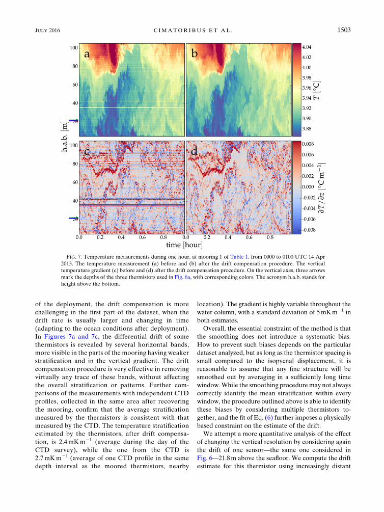
of the deployment, the drift compensation is more

challenging in the first part of the dataset, when the

drift rate is usually larger and changing in time

(adapting to the ocean conditions after deployment).

In Figures 7a and 7c, the differential drift of some

thermistors is revealed by several horizontal bands,

more visible in the parts of the mooring having weaker

stratification and in the vertical gradient. The drift

compensation procedure is very effective in removing

virtually any trace of these bands, without affecting

the overall stratification or patterns. Further com-

parisons of the measurements with independent CTD

profiles, collected in the same area after recovering

the mooring, confirm that the average stratification

measured by the thermistors is consistent with that

measured by the CTD. The temperature stratification

estimated by the thermistors, after drift compensa-

tion, is 2.4mKm21 (average during the day of the

CTD survey), while the one from the CTD is

2.7mKm21 (average of one CTD profile in the same

depth interval as the moored thermistors, nearby

location). The gradient is highly variable throughout the

water column, with a standard deviation of 5mKm21 in

both estimates.

Overall, the essential constraint of the method is that

the smoothing does not introduce a systematic bias.

How to prevent such biases depends on the particular

dataset analyzed, but as long as the thermistor spacing is

small compared to the isopycnal displacement, it is

reasonable to assume that any fine structure will be

smoothed out by averaging in a sufficiently long time

window.While the smoothing proceduremay not always

correctly identify the mean stratification within every

window, the procedure outlined above is able to identify

these biases by considering multiple thermistors to-

gether, and the fit of Eq. (6) further imposes a physically

based constraint on the estimate of the drift.

We attempt a more quantitative analysis of the effect

of changing the vertical resolution by considering again

the drift of one sensor—the same one considered in

Fig. 6—21.8m above the seafloor. We compute the drift

estimate for this thermistor using increasingly distant

FIG. 7. Temperature measurements during one hour, at mooring 1 of Table 1, from 0000 to 0100 UTC 14 Apr

2013. The temperature measurement (a) before and (b) after the drift compensation procedure. The vertical

temperature gradient (c) before and (d) after the drift compensation procedure. On the vertical axes, three arrows

mark the depths of the three thermistors used in Fig. 6a, with corresponding colors. The acronym h.a.b. stands for

height above the bottom.

JULY 2016 C IMATOR I BUS ET AL . 1503

sensors, rather than the two nearest ones alone. To bemore

specific, the sum S21,0,11k in Eqs. (7) and (8) is substituted

with S2m,0,1mk with m5 1, 2, 3, 4, . . . . Every estimate at

larger m mimics a lower vertical-resolution measurement.

The results of this exercise are shown in Fig. 8, which re-

ports the deviation from the original, full-resolution

(m5 1, 0.7m), drift estimate for m5 2, 3, 4, 6 (with a

vertical resolution of 1.4, 2.1, 2.8, and 4.2m, respectively).

From the figure we conclude that the method pro-

duces consistent results (with a precision of approxi-

mately 1mK) for vertical spacing up to approximately 3m.

For larger spacing, deviations from the full-resolution es-

timate are larger, and large fluctuations and a decreasing

trend in time are evident. Only the 4.2-m resolution is

shownas an example, but larger spacings provide similar or

worse results.

While this test gives some guidance for estimating the

vertical-resolution requirements in similar conditions,

we stress that these results should not be taken as gen-

eral. The resolution requirements will change markedly

with—to name a few examples—stratification, coher-

ence of vertical motions throughout the mooring, pres-

ence of strong horizontal gradients, etc. Ultimately,

only a careful analysis of the results obtained from a

particular mooring can provide an answer.

4. Examples of applications

We now briefly present two other applications of the

described procedure, using data from two other moor-

ings. First, we consider data from mooring 2 in Table 1,

deployed immediately after mooring 1 at a nearby,

deeper location. This dataset was used and described in

more detail in Cimatoribus et al. (2014) and van Haren

et al. (2015). This mooring used 140 thermistors of dif-

ferent ages, attached with a 1-m spacing between them.

Because of the deeper location, stratification is weaker.

Furthermore, battery failures and calibration issues af-

flicted this deployment, with 7 out of 140 thermistors

providing either unreadable or unusable data (white

stripes in Figs. 10a and 10b). These instrumental issues,

in combination with the weaker stratification, make

this a more challenging test for the drift compensation

procedure. The drift compensation procedure is per-

formed in the sameway as formooring 1, and it performs

time averaging in windows of 1 day but uses a poly-

nomial of degree 3 (instead of 4) as a guess of the real

stratification, since stratification is closer to linear at this

location. The drift of thermistors next to a missing one is

estimated using the available data alone; that is, no in-

terpolation is performed, and no sensors other than the

nearest ones are used.

Figure 9 shows an example of the drift estimation and

fit for the thermistor 51m above the seafloor. We see

that also in this case the drift is extracted and fitted re-

liably, with the negative drift rate identified from the

initial estimates (blue line in Fig. 9a) despite a nearby

thermistor having a stronger, opposite trend (red line in

Fig. 9a). Figure 10 confirms that the drift compensation

is effectively removing the drift from the observations,

and it shows that the procedure is not significantly af-

fected by the lack of data from some of the thermistors.

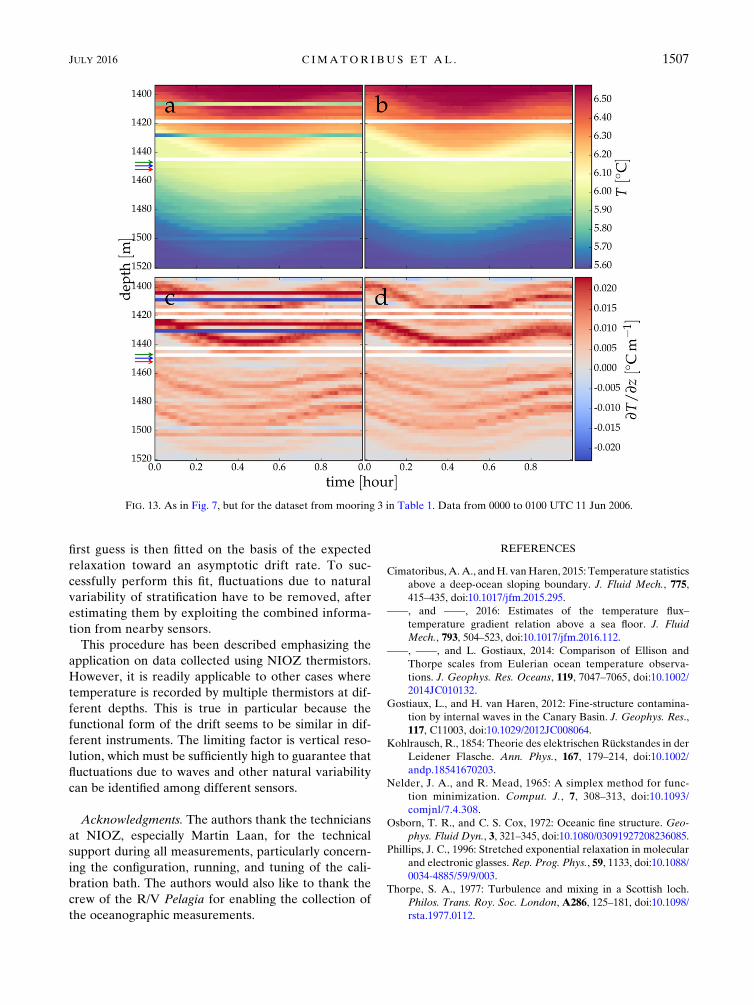
The last dataset considered has been collected be-

tween years 2006 and 2007 using older, NIOZ3, therm-

istors. This dataset was described in more detail in

FIG. 8. Estimate of the error on the drift reducing vertical reso-

lution. Different colors refer to different vertical resolutions (see

legend), obtained by subsampling in the vertical direction the

dataset of mooring 1 (Table 1). The drift estimate is computed for

the sensor 21.8m above the seafloor; see text for details.FIG. 9. As in Fig. 6, but for the dataset from mooring 2 in Table 1.

(a) Data from thermistors at a height above the seafloor of 55 (red),

56 (blue) and 57m (green). (b) Drift estimation for thermistor 56.

1504 JOURNAL OF ATMOSPHER IC AND OCEAN IC TECHNOLOGY VOLUME 33

van Haren et al. (2009), van Haren and Gostiaux (2009),

and Gostiaux and van Haren (2012). The mooring was

anchored in deep water (5275m), but the thermistors

were attached below a top buoy at a shallower depth,

approximately 1500m. The water column is more

stratified at this depth than in the other two moorings.

However, the calibration had to be performed in the

field at the time of the deployment, using concurrent

CTD measurements, since the calibration bath had not

been built yet. This posed stronger limitations on the

accuracy of the thermistor measurements. Furthermore,

some of these older thermistors suffered from an extreme

drift (in particular, the thermistor at 1410m in Figs. 11

and 13a). Finally, during the long deployment, some

thermistors failed due to battery depletion, so that not

every time series has the same length.

Despite these issues, the drift-compensating pro-

cedure can still be applied successfully, with minimal

changes. In particular, a smoothed spline is used in this

case rather than a polynomial fit for the initial esti-

mation of stratification, since the vertical temperature

gradient at this depth has more vertical structure

than in the deeper moorings (see Fig. 11). The drift

estimation is then performed first on the thermistor

with the strong drift at 1410m alone. This thermistor

has a drift of more than 18C in one year, and for this

reason its drift can be estimated without removing the

fluctuations, which are much smaller than the total

drift. Then, the drift of all other thermistors can be

estimated as done for the other moorings. This two-

step procedure enables the correct estimation of the

drift of the sensors adjacent to the one with extreme

drift, which would otherwise suffer from a biased esti-

mation of the fluctuating part.

Figure 12 shows the drift identification and fit for the

thermistor at 1450m. Nearby thermistors (red and

green lines) stop measuring before this thermistor

(black line), but this does not affect the drift estimation

significantly, because the drift rate has approximately

reached its asymptotic value by the time the other

thermistors stop. Note that the fluctuations (black line)

show a clear positive trend, which can be attributed to

the passage of a warm mesoscale structure at the

mooring location when the complete dataset is consid-

ered (van Haren et al. 2009). This trend is correctly in-

cluded in the common fluctuations and thus removed

FIG. 10. As in Fig. 7, but for the dataset from mooring 2 in Table 1. Data from 1200 to 1300 UTC 13 Aug 2013. The

acronym h.a.b. stands for height above the bottom.

JULY 2016 C IMATOR I BUS ET AL . 1505

from the drift estimate (i.e., it is left in the natural

temperature variation signal).

The fit represents the drift very well also in this case.

We note that these older thermistors generally have

higher drift rates and that the drift is often fitted suffi-

ciently well by a straight line in this dataset. Despite the

challenges encountered in processing this last dataset,

the results of the drift compensation are convincing

(Fig. 13), even at the beginning of the deployment. The

temperature stratification is negative in large parts of

this dataset due to the density compensation of salinity

variations at this location.

5. Summary and concluding remarks

We presented a characterization of the drift of the

temperature sensors designed at NIOZ and used in

several oceanographic moorings. The characterization

is done in the custom-built calibration bath of NIOZ.

The laboratory experiment supports the hypothesis

that the drift rate relaxes in time toward an asymptotic

value, which is itself a function of temperature. Using

this information, we develop a procedure to estimate

the drift rate of thermistors deployed in the field,

where no reference temperature measurements are

available. This procedure implies a guess of the aver-

age stratification computed from the thermistor mea-

surements in independent time windows, by means of a

smoothed interpolation. The drift estimated from this

FIG. 11. As in Fig. 5, but for the dataset from mooring 3 in Table 1. Data are 1-day averages from 27 Oct 2006.

FIG. 12. As in Fig. 6, but for the dataset frommooring 3 inTable 1.

(a)Data from thermistors at a depth of 1452 (red), 1449.5 (blue), and

1447m (green).

1506 JOURNAL OF ATMOSPHER IC AND OCEAN IC TECHNOLOGY VOLUME 33

first guess is then fitted on the basis of the expected

relaxation toward an asymptotic drift rate. To suc-

cessfully perform this fit, fluctuations due to natural

variability of stratification have to be removed, after

estimating them by exploiting the combined informa-

tion from nearby sensors.

This procedure has been described emphasizing the

application on data collected using NIOZ thermistors.

However, it is readily applicable to other cases where

temperature is recorded by multiple thermistors at dif-

ferent depths. This is true in particular because the

functional form of the drift seems to be similar in dif-

ferent instruments. The limiting factor is vertical reso-

lution, which must be sufficiently high to guarantee that

fluctuations due to waves and other natural variability

can be identified among different sensors.

Acknowledgments. The authors thank the technicians

at NIOZ, especially Martin Laan, for the technical

support during all measurements, particularly concern-

ing the configuration, running, and tuning of the cali-

bration bath. The authors would also like to thank the

crew of the R/V Pelagia for enabling the collection of

the oceanographic measurements.

REFERENCES

Cimatoribus,A.A., andH. vanHaren, 2015: Temperature statistics

above a deep-ocean sloping boundary. J. Fluid Mech., 775,

415–435, doi:10.1017/jfm.2015.295.

——, and ——, 2016: Estimates of the temperature flux–

temperature gradient relation above a sea floor. J. Fluid

Mech., 793, 504–523, doi:10.1017/jfm.2016.112.

——, ——, and L. Gostiaux, 2014: Comparison of Ellison and

Thorpe scales from Eulerian ocean temperature observa-

tions. J. Geophys. Res. Oceans, 119, 7047–7065, doi:10.1002/2014JC010132.

Gostiaux, L., and H. van Haren, 2012: Fine-structure contamina-

tion by internal waves in the Canary Basin. J. Geophys. Res.,

117, C11003, doi:10.1029/2012JC008064.Kohlrausch, R., 1854: Theorie des elektrischen Rückstandes in der

Leidener Flasche. Ann. Phys., 167, 179–214, doi:10.1002/

andp.18541670203.

Nelder, J. A., and R. Mead, 1965: A simplex method for func-

tion minimization. Comput. J., 7, 308–313, doi:10.1093/

comjnl/7.4.308.

Osborn, T. R., and C. S. Cox, 1972: Oceanic fine structure. Geo-

phys. Fluid Dyn., 3, 321–345, doi:10.1080/03091927208236085.

Phillips, J. C., 1996: Stretched exponential relaxation in molecular

and electronic glasses. Rep. Prog. Phys., 59, 1133, doi:10.1088/

0034-4885/59/9/003.

Thorpe, S. A., 1977: Turbulence and mixing in a Scottish loch.

Philos. Trans. Roy. Soc. London, A286, 125–181, doi:10.1098/

rsta.1977.0112.

FIG. 13. As in Fig. 7, but for the dataset from mooring 3 in Table 1. Data from 0000 to 0100 UTC 11 Jun 2006.

JULY 2016 C IMATOR I BUS ET AL . 1507

van Haren, H., and L. Gostiaux, 2009: High-resolution open-ocean

temperature spectra. J.Geophys. Res., 114, C05005, doi:10.1029/

2008JC004967.

——, and——, 2010: A deep-oceanKelvin-Helmholtz billow train.

Geophys. Res. Lett., 37, L03605, doi:10.1029/2009GL041890.

——, M. Laan, D.-J. Buijsman, L. Gostiaux, M. G. Smit, and

E. Keijzer, 2009: NIOZ3: Independent temperature sensors

sampling yearlong data at a rate of 1Hz. IEEE J. Oceanic

Eng., 34, 315–322, doi:10.1109/JOE.2009.2021237.

——, L. Gostiaux, M. Laan, M. van Haren, E. van Haren, and

L. J. A. Gerringa, 2012: Internal wave turbulence near a texel

beach. PLoSOne, 7, e32535, doi:10.1371/journal.pone.0032535.

——,A.Cimatoribus, andL.Gostiaux, 2015:Where large deep-ocean

waves break. Geophys. Res. Lett., 42, 2351–2357, doi:10.1002/

2015GL063329.

Wood, S. D., B.W.Mangum, J. J. Filliben, and S. B. Tillet, 1978:An

investigation of stability of thermistors. J. Res. Natl. Bur.

Stand., 83, 247–263, doi:10.6028/jres.083.015.

1508 JOURNAL OF ATMOSPHER IC AND OCEAN IC TECHNOLOGY VOLUME 33