A PRO-FORMA APPROACH TO CAR-CARRIER DESIGN
98
A PRO-FORMA APPROACH TO CAR-CARRIER DESIGN Richardt Benade A dissertation submitted to the Faculty of Engineering and the Built Environment, of the University of the Witwatersrand, in fulfilment of the requirements for the degree of Master of Science in Engineering Johannesburg 2016
Transcript of A PRO-FORMA APPROACH TO CAR-CARRIER DESIGN

A PRO-FORMA APPROACH TO
CAR-CARRIER DESIGN
Richardt Benade
A dissertation submitted to the Faculty of Engineering and the Built Environment, of the
University of the Witwatersrand, in fulfilment of the requirements for the degree of
Master of Science in Engineering
Johannesburg 2016

DECLARATION
I declare that this dissertation is my own unaided work. It is being submitted to the degree
of Master of Science in Engineering to the University of the Witwatersrand,
Johannesburg. It has not been submitted before for any degree or examination to any
other University. I further declare that I have been an employee of the Council for
Scientific and Industrial Research during the course of my post-graduate studies.
…………………………
(Signature of Candidate)
29th day of February, year 2016

i
ABSTRACT
To mitigate accidents, reduce loss of life and to protect road infrastructure, it is important that heavy
vehicles are regulated. Regulatory frameworks can be divided into two main groups: prescriptive and
non-prescriptive. The prescriptive regulatory framework is currently the norm in South Africa and the
majority of countries worldwide. Road safety in this framework is governed by placing constraints on
vehicle mass and dimensions. These parameters can be measured by the law enforcer and if these are
found to exceed prescribed limits, the vehicle is deemed unfit for road use. Although such a legislative
framework is simple to enforce and manage, prescriptive standards inherently impose constraints on
innovative design and productivity, without guaranteeing vehicle safety. An alternative regulatory
framework is the performance-based standards (PBS) framework. This alternative non-prescriptive
framework provides more freedom and directly (as opposed to indirectly) regulates road safety. Limits
regarding overall length and gross combination mass (GCM) are relaxed but other safety-ensuring
standards are required to be met. These standards specify the safety performance required from the
operation of a vehicle on a network rather than prescribing how the specified level of performance is to be
achieved. On 10 March 2014, the final version of the South African roadmap for car-carriers was
accepted by the Abnormal Loads Technical Committee. The roadmap specified that, from thereon, all car-
carriers registered after 1 April 2013 would only be granted overall length and height exemptions (which
logistics operators have insisted are essential to remain in business) if the design is shown to meet level 1
PBS performance requirements. This resulted in an increased demand for car-carrier PBS assessments.
One significant drawback of the PBS approach is the time and expertise required for conducting PBS
assessments. In this work a pro-forma approach is developed for assessing future car-carrier designs in
terms of their compliance with the South African PBS pilot project requirements. First, the low-speed
PBS were considered and a low-speed pro-forma design was developed by empirically deriving equations
for frontal swing, tail swing and low speed swept path. These were incorporated into a simplified tool for
assessing the low-speed PBS compliance of car-carriers using a top-view drawing of the design.
Hereafter, the remaining PBS were considered, incorporating additional checks to be performed when
evaluating a potential vehicle. It was found necessary to specify a minimum drive axle load in order to
meet the startability, gradeability and acceleration capability standards. The required drive axle load was
determined as 19.3% of the GCM. It was confirmed that the static rollover threshold performance can
accurately be predicted by means of the applicable New Zealand Land Transport Rule method. The study
is limited to 50/50-type car-carriers, however the methodology developed will be used to construct
assessment frameworks for short-long and tractor-and-semitrailer combinations. The pro-forma approach
offers a cost-effective and simplified alternative to conventional TruckSim® PBS assessments. This
simplified approach can significantly benefit the PBS pilot project by offering a sustainable way to
investigate the PBS conformance of proposed car-carriers.

ii
PUBLISHED WORK
Aspects of this dissertation have been published:
Conference Paper- South African Transport Conference July 2015
R. Benade, F. Kienhöfer, R. Berman, and P. A. Nordengen, “A Pro-Forma Design for Car-Carriers : Low-
Speed Performance-Based Standards,” in Proceedings of the 34th South African Transport Conference,
pp. 253–265, 2015.

iii
ACKNOWLEDGEMENTS
I would like to thank my supervisor, Dr Frank Kienhöfer for his continuing support and guidance.
Thanks to the following individuals for offering technical guidance
Robert Berman (CSIR)
Christopher de Saxe (CSIR/University of Cambridge)
Dr Paul Nordengen (CSIR)
Dr John de Pont (Ternz, New Zealand)
Thanks to the following industry partners for providing the necessary technical information
Andrew Colepeper (Unipower Natal)
Justin Michau (Lohr)
Gary Spowart (Volvo)
Clifford Steele (Renault/Volvo)
Christo Kleynhans (Daimler)
Gunther Heyman (BPW Axles)

iv
TABLE OF CONTENTS
TABLE OF CONTENTS ..................................................................................................................... iv
LIST OF FIGURES ............................................................................................................................. vi
LIST OF TABLES ............................................................................................................................. viii
ABBREVIATIONS .............................................................................................................................. ix
SYMBOLS ............................................................................................................................................. x
1. INTRODUCTION .......................................................................................................................... 1
1.1. Prescriptive regulation ............................................................................................................ 1
1.2. Australian performance-based standards (PBS) ..................................................................... 2
1.3. PBS demonstration project: South Africa ............................................................................... 3
1.4. Literature review ..................................................................................................................... 5
1.4.1. Pro-forma approach .................................................................................................... 5
1.4.2. Influence of typical design features on PBS ............................................................... 7
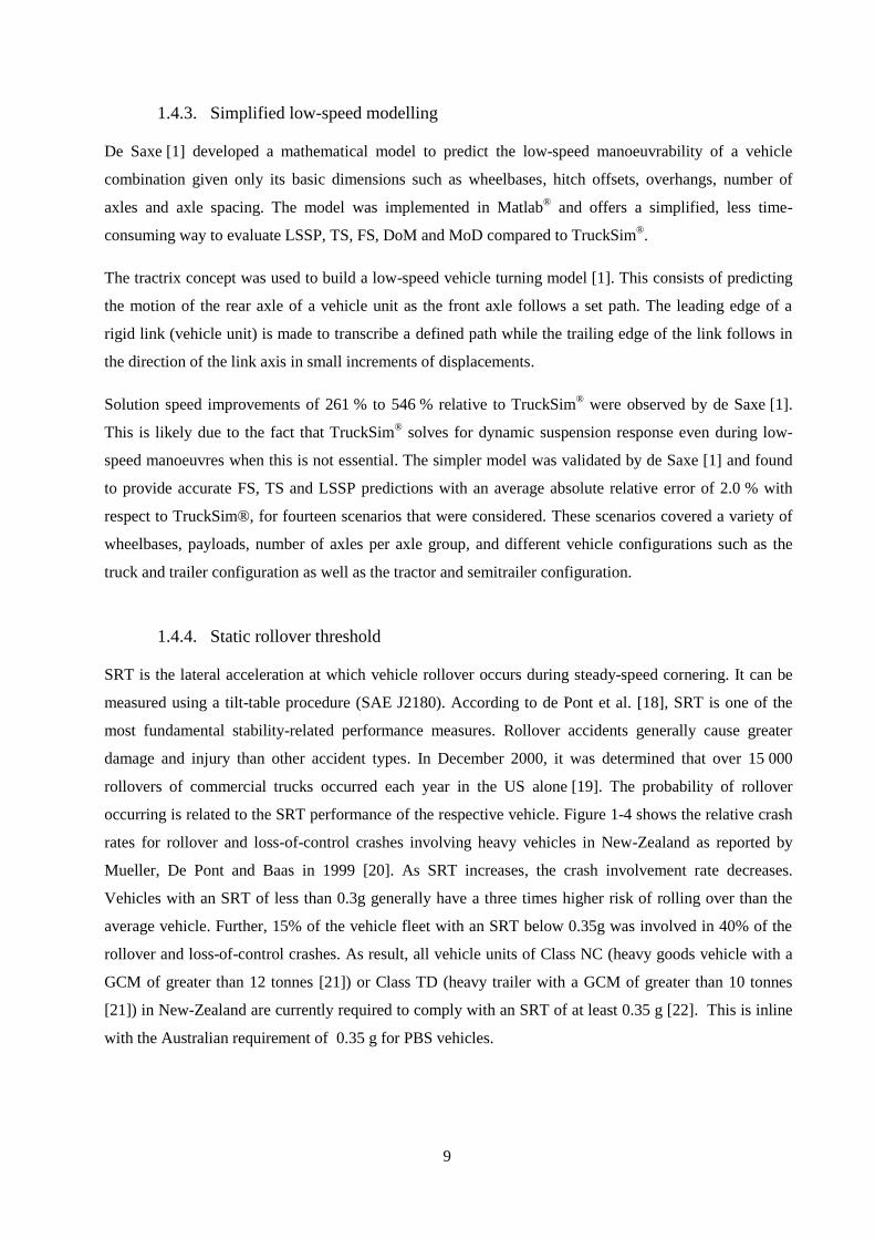
1.4.3. Simplified low-speed modelling ................................................................................. 9
1.4.4. Static rollover threshold.............................................................................................. 9
1.5. Purpose of the study .............................................................................................................. 14
1.6. Overview of remaining chapters ........................................................................................... 15
2. PBS ASSESSMENT OF A COMMERCIAL CAR-CARRIER ............................................... 16
2.1. Vehicle description ............................................................................................................... 16
2.2. Payload description ............................................................................................................... 18
2.3. PBS standards and assessment results: commercial car-carrier ............................................ 19
2.3.1. Startability ................................................................................................................ 19
2.3.2. Gradeability A .......................................................................................................... 20
2.3.3. Gradeability B .......................................................................................................... 21
2.3.4. Acceleration capability ............................................................................................. 21
2.3.5. Tracking ability on a straight path ............................................................................ 22
2.3.6. Low speed swept path............................................................................................... 24
2.3.7. Frontal swing ............................................................................................................ 25
2.3.8. Tail swing ................................................................................................................. 26
2.3.9. Steer tyre friction demand ........................................................................................ 28
2.3.10. Static rollover threshold............................................................................................ 30

v
2.3.11. Rearward amplification ............................................................................................ 30
2.3.12. High-speed transient offtracking .............................................................................. 32
2.3.13. Yaw damping coefficient.......................................................................................... 33
2.3.14. Summary and discussion of results .......................................................................... 34
2.4. Chapter conclusion: PBS assessment of a commercial car-carrier ....................................... 36
3. DEVELOPMENT OF A PRO-FORMA DESIGN .................................................................... 37
3.1. Low-speed PBS ..................................................................................................................... 37
3.1.1. Validation: low-speed mathematical model ............................................................. 38
3.1.2. Development of a low-speed pro-forma ................................................................... 40
3.2. Remaining PBS ..................................................................................................................... 69
3.2.1. Typical PBS performance of 50/50-type car-carriers ............................................... 70
3.2.2. Startability, gradeability A and acceleration capability ............................................ 72
3.2.3. Static rollover threshold............................................................................................ 74
4. CONCLUSION ............................................................................................................................. 77
5. RECOMMENDATIONS FOR FURTHER WORK ................................................................. 78
REFERENCES .................................................................................................................................... 79
...................................................................................................................................... 82 APPENDIX A

vi
LIST OF FIGURES
Figure 1-1 Types of South African car-carriers (a) tractor and semitrailer, (b) truck and trailer [1] ........... 4
Figure 1-2 Steady state low-speed turning of a 2-axle vehicle..................................................................... 6
Figure 1-3 Pro-forma design: truck and full trailer [14] ............................................................................... 7
Figure 1-4 Relative crash rate versus SRT [18] ......................................................................................... 10
Figure 1-5 Vehicle roll notation: land transport rule method [22] ............................................................. 11
Figure 1-6 Suspension and axle lash [22]................................................................................................... 12
Figure 2-1 Mercedes Benz Actros 2541 with Macroporter trailer [24] ...................................................... 16
Figure 2-2 Worst-case payload: truck ........................................................................................................ 19
Figure 2-3 Worst-case payload: trailer ....................................................................................................... 19
Figure 2-4 Startability: commercial car-carrier .......................................................................................... 20
Figure 2-5 Gradeability B: commercial car-carrier .................................................................................... 21
Figure 2-6 Acceleration capability: commercial car-carrier....................................................................... 22
Figure 2-7 Tracking ability on straight path: swept width [4] .................................................................... 23
Figure 2-8 Tracking ability on a straight path: commercial car-carrier...................................................... 23
Figure 2-9 Manoeuvre and measurement of LSSP [4] ............................................................................... 24
Figure 2-10 Front section of truck (top view, obtained from Unipower) ................................................... 24
Figure 2-11 Low speed swept path: commercial car-carrier ...................................................................... 25
Figure 2-12 Measuring frontal swing (left) and outside wheel reference point (right) [4] ........................ 25
Figure 2-13 Frontal swing: commercial car-carrier .................................................................................... 26
Figure 2-14 Measuring tail swing [4] ......................................................................................................... 27
Figure 2-15 Rear section of trailer (top view, obtained from Unipower) ................................................... 27
Figure 2-16 Rear section of truck (top view, obtained from Unipower) .................................................... 28
Figure 2-17 Tail swing: commercial car-carrier ......................................................................................... 28
Figure 2-18 Steer tyre friction demand: commercial car-carrier ................................................................ 29
Figure 2-19 Static rollover threshold: commercial car-carrier ................................................................... 30
Figure 2-20 Rearward amplification: commercial car-carrier .................................................................... 31
Figure 2-21 High-speed, single lane change manoeuvre and measuring HSTO [4] .................................. 32
Figure 2-22 High-speed transient offtracking: commercial car-carrier ...................................................... 32
Figure 2-23 Amplitudes for damping ratio calculation [4]......................................................................... 33
Figure 2-24 Yaw damping coefficient: commercial car-carrier ................................................................. 34

vii
Figure 2-25 Top-laden load case of the truck and the trailer (decks lowered) ........................................... 35
Figure 3-1 Input parameters required by LSMM [1] .................................................................................. 38
Figure 3-2 Illustration of LSMM parameters (modified from Unipower drawings) .................................. 39
Figure 3-3 PSF wrt FS for increased parameters........................................................................................ 41
Figure 3-4 PSF wrt TS for increased (left) and decreased (right) parameters ............................................ 42
Figure 3-5 PSF wrt LSSP for increased parameters ................................................................................... 43
Figure 3-6 Performance of designs tested (original IEwid bounds) .............................................................. 45
Figure 3-7 Performance of designs tested (revised IEwid bounds) .............................................................. 45
Figure 3-8 Performance of designs tested (original WB1) .......................................................................... 47
Figure 3-9 Performance of designs tested (updatedWB1) ........................................................................... 48
Figure 3-10 Grid search of critical FC locations ........................................................................................ 49
Figure 3-11 Shaped search of critical FC locations .................................................................................... 50
Figure 3-12 Frontal corner boundary ......................................................................................................... 51
Figure 3-13 Grid search of critical RC locations ........................................................................................ 52
Figure 3-14 Shaped search of critical RC locations ................................................................................... 52
Figure 3-15 Rear corner boundary ............................................................................................................. 53
Figure 3-16 Grid search of critical RC locations ........................................................................................ 54
Figure 3-17 Shaped search of critical RC locations ................................................................................... 55
Figure 3-18 Rear corner boundary ............................................................................................................. 56
Figure 3-19 Grid search of critical FC locations in terms of LSSP ............................................................ 57
Figure 3-20 Shaped search of critical FC locations in terms of LSSP ....................................................... 57
Figure 3-21 Volvo FM62TT hauling the Macroporter MK3 ..................................................................... 59
Figure 3-22 Assessment tool: low-speed PBS (input) ................................................................................ 67
Figure 3-23 Assessment tool: low-speed PBS (output) .............................................................................. 68
Figure 3-24 Assessment of the Mercedes-Benz Actros 2541+ Macroporter MK3 .................................... 68
Figure 3-25 Assessment of the Volvo FM 62TT + Macroporter MK3 ...................................................... 68
Figure 3-26 Assessment of the Volvo FM400 + Lohr MHR 3.10 EHR 2.10 ............................................ 68
Figure 3-27 Assessment of the Mercedes-Benz Actros 2541-54 + Lohr MHR 3.30 AS D1 2.03 XS ....... 69
Figure 3-28 Assessment of the Scania P410 LB 6x2 MNA + Lohr MHR EHR ........................................ 69
Figure 3-29 Startability for various drive axle loads .................................................................................. 73
Figure 3-30 Gradeability A for various drive axle loads ............................................................................ 73
Figure 3-31 Acceleration capability for various drive axle loads .............................................................. 74

viii
LIST OF TABLES
Table 1-1 Truck crash statistics for various countries [2] ............................................................................ 1
Table 1-2 Safety standards and their description [1] .................................................................................... 2
Table 1-3 Influence of typical design features on PBS [17] ........................................................................ 8
Table 2-1 Specification of truck ................................................................................................................. 17
Table 2-2 Summarised axle and suspension data of combination .............................................................. 17
Table 2-3 Unladen sprung mass properties ................................................................................................ 17
Table 2-4 Payload properties ...................................................................................................................... 18
Table 2-5 Unsprung mass properties .......................................................................................................... 18
Table 2-6: PBS assessment results ............................................................................................................. 35
Table 2-7 SRT and high-speed PBS assessment results: additional load cases ......................................... 36
Table 3-1 Input parameters required by LSMM [1] ................................................................................... 37
Table 3-2 LSMM input parameters: commercial car-carrier...................................................................... 39
Table 3-3 LSMM validation results: Macroporter ..................................................................................... 39
Table 3-4 Parameter limits wrt FS ............................................................................................................. 41
Table 3-5 Parameter limits wrt TS ............................................................................................................. 42
Table 3-6 Parameter limits wrt LSSP ......................................................................................................... 43
Table 3-7 Preliminary low-speed pro-forma .............................................................................................. 44
Table 3-8 Parameter combinations tested................................................................................................... 46
Table 3-9 Assessing a new concept design using pro-forma design .......................................................... 60
Table 3-10 Vehicle parameters of five 50/50- type car-carriers ................................................................. 61
Table 3-11 Customisable pro-forma limits................................................................................................. 62
Table 3-12 Parameter description for FS prediction .................................................................................. 63
Table 3-13 Parameter description for LSSP prediction .............................................................................. 64
Table 3-14 Parameter description for TS (truck) prediction ...................................................................... 65
Table 3-15 Parameter description for TS (trailer) prediction ..................................................................... 66
Table 3-16 PBS standards to consider ........................................................................................................ 70
Table 3-17 PBS performance of five commercial 50/50 car-carriers ......................................................... 71
Table 3-18 SRT performance using various predictor tools...................................................................... 76

ix
ABBREVIATIONS
AC Acceleration capability
ALTC Abnormal Loads Technical Committee
CoG Centre of gravity
CSIR Council for Scientific and Industrial Research
DoM Difference of maxima
FC Front corner
FS Frontal swing
GCM Gross combination mass
GrA Gradeability A
GrB Gradeability B
HSTO High-speed transient offtracking
IRI International Roughness Index
LSMM Low-speed mathematical model
LSSP Low-speed swept path
MoD Maximum of difference
NHVR National Heavy Vehicle Regulator
NRTA National Road Traffic Act
NTC National Transport Commission
NZLTR New Zealand Land Transport Rule
OEM Original equipment manufacturer
PBS Performance-based standards
PSF Parameter significance factor
rrcc Rear roll-coupled unit
RA Rearward amplification
RCC Roadmap for car-carriers
RTMS Road Transport Management System
SASTRP South African Smart Truck Review Panel
SRT Static rollover threshold
St Startability
STFD Steer tyre friction demand
TASP Tracking ability on a straight path
TS Tail swing
UMTRI University of Michigan Transportation Research Institute
VDAM Vehicle Dimensions and Mass
YDC Yaw damping coefficient

x
SYMBOLS
Steer tyre friction demand
𝑭𝒙𝒏 Longitudinal tyre force at nth
tyre (N)
𝑭𝒚𝒏 Lateral tyre force at nth
tyre (N)
𝑭𝒛𝒏 Vertical tyre force at nth
tyre (N)
𝑵 Number of tyres on steer axle or axle group
𝝁𝒑𝒆𝒂𝒌 Peak value of prevailing tyre/road friction
Low-speed mathematical model
T Outside track width of steer tyres (m)
WBj Geometric wheelbase (m)
FClong,j Longitudinal position of front corner (positive forward of the
steer axle/hitch) (m)
FCwid,j Vehicle width at front corner (m)
RClong,j Longitudinal position of rear corner (positive rearward of the
steer axle/hitch) (m)
RCwid,j Vehicle width at rear corner (m)
nj Number of non-steering rear axles
dj Axle spacing between non-steering rear axles (m)
IEwid,j Vehicle width at inner edge (m)
Hj Hitch point location (positive rearward of the steer axle/hitch)
(m)
Static rollover threshold
T Track width (m)
H CoG height of entire vehicle including payload (m)
WP Payload mass (kg)
We Empty vehicle mass (kg)
Hp Height of CoG of payload (m)
Ms Sprung mass (kg)
hc Sprung mass CoG height from ground (m)
hb Roll centre height from ground (m)
kr Composite suspension roll stiffness (Nm/rad)
M Total mass (kg)
Mu Unsprung mass (kg)
ha Axle CoG height from ground (m)
kt Tyre stiffness (N/m)
ks Spring stiffness (N/m)
t Suspension track (m)
kaux Auxiliary roll stiffness (Nm/rad)
θ Sprung mass roll angle (rad)
φ Axle roll angle (rad)
ζ Suspension roll angle (rad) due to lash

1
1. INTRODUCTION
Heavy vehicle regulation is imperative to mitigate accidents, reduce loss of life and to protect road
infrastructure. Regulatory frameworks can be divided into two main groups: prescriptive and non-
prescriptive.
1.1. Prescriptive regulation
The prescriptive regulatory framework is currently the norm in South Africa and the majority of countries
worldwide. Road safety in this framework is governed by placing constraints on vehicle mass and
dimensions. These parameters can be measured by the law enforcer and if these are found to exceed
prescribed limits, the vehicle is deemed unfit for road use. Although such a legislative framework is
simple to enforce and manage, prescriptive standards inherently impose constraints on innovative design
and productivity. Further, prescriptive standards do not guarantee acceptable levels of vehicle safety or
road wear [1]. Under prescriptive regulation, South Africa has shown undesirable crash statistics
compared to a number of other countries, also operating under prescriptive regulation [2]. Table 1-1
shows the number of fatalities per 100 million kilometres travelled by trucks for various countries world-
wide. South Africa showed the largest number of fatalities per 100 million kilometres (12.5), over four
times that of Denmark- the country with the second highest number. Based on the 2013 State of Logistics
survey, logistics costs make up 12.5% of South Africa’s gross domestic product, with transportation
accounting for 61.6% of this [3]. Proper regulation of heavy vehicles thus plays a significant role in
maintaining a healthy economy. An alternative regulatory framework is performance-based standards
(PBS), a non-prescriptive framework as discussed in the following section.
Table 1-1 Truck crash statistics for various countries [2]
Country Fatalities per 100 million
kilometres of truck travel Year
South Africa 12.5 2005
Switzerland 0.8 2005
Belgium 1.9 2005
United States 1.5 2005
France 2.0 2005
Germany 1.5 2006
Australia 1.7 2005
Canada 2.0 2005
Sweden 1.6 2005
Great Britain 1.7 2005
Denmark 3.0 2004

2
1.2. Australian performance-based standards (PBS)
In Australia, the National Transport Commission (NTC) established a performance-based
standards (PBS) scheme [4] which is now managed by the National Heavy Vehicle Regulator (NHVR).
This alternative legislative framework or PBS scheme provides more freedom and directly (as opposed to
indirectly) regulates road safety [1]. Limits regarding overall length and gross combination mass (GCM)
are relaxed but other safety-ensuring standards are required to be met. These standards specify the
performance required from the operation of a vehicle on a network rather than prescribing how the
specified level of performance is to be achieved [5].
The PBS scheme governs longitudinal performance, low-speed directional performance and high-speed
directional performance of heavy vehicles. A summary of the standards is given in Table 1-2.
Longitudinal performance (described by standards 1 to 3) is mainly affected by the GCM, engine capacity
and drivetrain characteristics of the vehicle. Low-speed directional performance (standards 4 to 7) is
mainly affected by the geometry of the vehicle such as length, width and axle positions. High-speed
directional performance (standards 8 to 12) is affected by the vehicle’s suspension characteristics, tyre
properties, centre of gravity (CoG) location and GCM. Most standards have four levels of compliance
whereas some standards, for example static rollover threshold (SRT), simply have a pass or fail
criterion [4]. The achieved performance level designates the allowable route clearance.
Table 1-2 Safety standards and their description [1]
Manoeuvre Safety Standard Description
Accelerate from rest on an incline 1. Startability (St) Maximum upgrade on which the vehicle
can start from rest.
Maintain speed on an incline
2.a. Gradeability A (GrA) Maximum upgrade on which the vehicle
can maintain forward motion.
2.b. Gradeability B (GrB) Maximum speed that the vehicle can
maintain on a 1% upgrade
Cover 100 m from rest 3. Acceleration capability (AC) Intersection/rail crossing clearance times.
Low-speed 90° turn
4. Low-speed swept path (LSSP) “Corner cutting” of long vehicles.
5. Frontal swing (FS) Swing-out of the vehicle’s front corner.
5a. Maximum of Difference (MoD) The difference in frontal swing-out of
adjacent vehicle units where one of the
units is a semitrailer. 5b. Difference of Maxima (DoM)
6. Tail swing (TS) Swing-out of the vehicle’s rear corner.
7. Steer-tyre friction demand (STFD) The maximum friction utilised by the steer-
tyres.
Straight road of specified
roughness and cross-slope
8. Tracking ability on a straight path
(TASP)
Total road width utilised by the vehicle as it
responds to the uneven road at speed.
Constant radius turn (increasing
speed) or tilt-table testing 9. Static rollover threshold (SRT)
The maximum steady lateral acceleration a
vehicle can withstand before rolling.
Single lane-change
10. Rearward amplification (RA) “Whipping” effect of trailing units.
11. High-speed transient offtracking
(HSTO) “Overshoot” of the rearmost trailing unit.
Pulse steer input 12. Yaw damping coefficient (YDC) The rate at which yaw oscillations settle.

3
1.3. PBS demonstration project: South Africa
The Australian PBS scheme has been adapted and operated as a demonstration project in South Africa [6]
in parallel with the prescriptive legislative framework that is defined by the National Road Traffic Act
(NRTA) [7]. The demonstration project has proved a fourfold benefit since its inception in 2004 [6]:
More economic payload transportation
Increased vehicle safety
Reduced road infrastructure damage
Reduced emissions
Heavy vehicle operators looking to participate in the project are required to be accredited with the Road
Transport Management Scheme (RTMS). This requirement is to ensure that the transport operator, and in
particular the relevant fleet, is being managed and operated in accordance with prescribed minimum
safety and loading standards [5]. The RTMS scheme aims to improve vehicle management through
audited self-regulation [6]. A further requirement is to show, usually through simulation, that the road
wear of the proposed vehicle is acceptable and that the vehicle complies with the Australian PBS
standards [5]. Road-wear assessments are conducted using the South African Mechanistic Pavement
Design Method [8]. The Council for Scientific and Industrial Research (CSIR) have developed a software
package, MePADS, to simplify the road-wear assessments. PBS assessments are generally conducted by
the CSIR or the University of the Witwatersrand using commercially available vehicle dynamics
simulation software such as TruckSim®. Assessments can also be done through Australian NTC-
accredited PBS assessors such as Advantia [9] and ARRB [10]. The South African Smart Truck Review
Panel (SASTRP), consisting of various industry, regulatory as well as academic partners evaluates the
assessments and approves or rejects the proposed applications on a bimonthly basis.
One significant drawback of the PBS approach is the time and expertise required for conducting PBS
assessments; gathering input data, developing models, analysing results and compiling reports. The back-
and-forth exchanging of design modifications between designers and PBS assessors, trying to arrive at a
PBS compliant design, is also particularly time-consuming. This is troublesome in South Africa, where
there are only four accredited PBS assessors while the industry is starting to show substantial interest in
the PBS project. The cost of one TruckSim® license, as quoted by Mechanical Simulation Corporation on
05 June 2015 was $36 000. Adding to the existing practical challenges of conducting PBS assessments,
this relates to roughly R480 000.
South African roads are travelled by mainly two types of car-carriers as shown in Figure 1-1. The tractor-
and-semitrailer combination (a) is typically used in short-haul applications whereas the truck-and-trailer
combination (b) is mainly used for long-haul applications. The truck-and-trailer combination has a further
classification; the so-called short-long, which can accommodate three passenger vehicles on the truck and

4
seven to ten passenger vehicles on the trailer, and the so-called 50/50 type, which can accommodate five
passenger vehicles on the truck and seven to eleven passenger vehicles on the trailer.
Figure 1-1 Types of South African car-carriers (a) tractor and semitrailer, (b) truck and trailer [1]
On 10 March 2014, the final version of the South African roadmap for car-carriers (RCC) was accepted
by the Abnormal Loads Technical Committee (ALTC) [11]. The RCC specified that, from thereon, all
car-carriers registered after 1 April 2013 would only be granted overall length and height exemptions if
the design is shown to meet level 1 PBS performance requirements. This exemption allows truck and
trailer car-carriers to operate up to an overall length of 23 m (including payload projection) and an overall
height of 4.6 m, slightly less strict than the NRTA’s limits of 22 m and 4.3 m respectively [7]. These
slightly relaxed limitations offer significant benefits to industry in terms of productivity and resulted in an
increased demand for car-carrier PBS assessments. One of the main challenges with car-carrier PBS
assessments is that each car-carrier design (superstructure and trailer) needs to be assessed with each
hauling unit that the operator aims to utilise as any change in suspension or other design characteristics
could potentially compromise compliance in terms of PBS. Currently, three commercial car-carrier
manufacturers Unipower (Natal), Lohr Transport Solutions ZA, and Rolfo South Africa have had PBS
assessments conducted in South Africa and have developed eight PBS car-carrier designs.
If each trailer design is assessed with three hauling units, this would require twenty-four assessments. If
each assessment is estimated to cost R66,000 in consulting fees, the PBS car-carrier assessments would
cost the industry R1,584,000. Apart from the financial burden, the PBS assessment process causes
significant delays in getting the vehicles on the road. Furthermore if a hauling unit model is updated then

5
this would require a new assessment. Unique PBS assessments for each unique tractor make and model
and trailer type is not a sustainable solution for the car-carrier industry.
1.4. Literature review
An overview will be given of studies implementing PBS in a semi-prescriptive manner, after which
findings of the influence of vehicle design features on PBS performance will be introduced. A
mathematical model that was developed for assessing the low-speed performance of combination vehicles
will be described. Lastly, the significance of the SRT standard and various existing prediction tools will
also be discussed.
1.4.1. Pro-forma approach
In New Zealand, a semi-prescriptive or “pro-forma” approach is followed where vehicle manufacturers
are offered designs indicating dimension ranges that are pre-approved using the relevant framework and
thus exempted from assessment [12]. A similar approach is followed in Australia where these vehicle
designs are referred to as “blueprints” [13]. Such an approach speeds up the process of approving PBS
vehicles significantly as less formal PBS assessments are required. If a manufacturer however decides on
a design that falls outside of the pre-approved bounds, a full PBS assessment is required. As yet, the
semi-prescriptive approach has not been attempted within the South African demonstration project.
In 2010, low-speed pro-forma designs were developed for three widely-used heavy vehicles in New
Zealand [14]. These included a truck and full trailer, B-train, and a truck and simple trailer. The term “full
trailer” implies that the trailer can fully support itself, having both front and rear running gear, as opposed
to a “semi-trailer” that requires vertical support from the towing vehicle as it has no front running
gear [15]. The “B” in “B-train” indicates a roll-coupled connection between the vehicle units, usually by
means of a fifth-wheel hitch [15]. Based on a legal vehicle, it was decided that the maximum swept width
(similar to LSSP) for the low-speed pro-forma design should be 7.6 m when executing a 120° turn at a
12.5 m radius.
As De Pont [14] explains, consider a 2-axle vehicle such as a car or small truck executing a steady-state
low-speed manoeuvre as shown in Figure 1-2 (modified from diagrams drawn by Gillespie [16] and De
Pont [14]). Note that the radius of the path followed by the front axle (R1) is greater than the radius of the
path followed by the rear axle (R2). The difference between R1 and R2 is known as off-tracking. R2 can be
calculated from R1 and WB using Pythagoras’ theorem.

6
Figure 1-2 Steady state low-speed turning of a 2-axle vehicle
When considering a combination vehicle, the same approach can be repeated for each vehicle unit to
calculate an equivalent wheelbase of the combination vehicle [14]:
2 2_equivalent i i
i i
WB WB Hitch Offset
(1-1)
Where:
iWB = wheelbase of vehicle unit 𝑖
_ iHitch Offset = distance between the rear axle and the coupling on vehicle unit 𝑖
The amount of off-tracking during a steady state constant radius turn can easily be calculated using the
equivalent wheelbase of a combination vehicle. During the 120° turn (that was modelled by De Pont [14])
as well as a 90° turn (as per the Australian PBS standards [4]), steady state is not likely reached according
to De Pont [14]. This means that the amount of off-tracking cannot be accurately predicted by the
equivalent wheelbase. As a substitute, multi-body dynamics computer simulation packages such as Yaw-
Roll were used to predict off-tracking. The equivalent wheelbase is however useful for identifying
improvements to vehicle combinations. As De Pont [14] explains, a lower equivalent wheelbase generally
results in less off-tracking allowing the following deductions to be made from Eq.(1-1):
Equally matched unit wheelbases produce less offtracking. For example two units with a 6 m
wheelbase produce a smaller equivalent wheelbase than a unit with an 8 m wheelbase and a unit
with a 4 m wheelbase.
Larger hitch offsets reduce offtracking (for both positive and negative offsets).
Figure 1-3 shows the pro-forma design that was developed for the truck and full trailer [14]. Through
some reasoning and modelling, semi-prescriptive limits were imposed on critical vehicle parameters in
order to comply with a maximum swept width limit of 7.6 m when executing a 120° turn at a 12.5 m
R2
WB

7
radius. A 22 m commercial truck-and-full-trailer combination was originally assessed and found to
comfortably meet the maximum swept width requirement. There was thus some scope to vary certain
parameters while still complying with the maximum swept width limit. Note that for all vehicles a front
vehicle width of 2.4 m was assumed. It was found that the truck forward length (distance from the rear
axis to the front of the vehicle) and trailer wheelbase could be increased to 7.5 m simultaneously as long
as the hitch offset remained above 2.6 m and the drawbar length was limited to 2.9 m. An amendment to
the Vehicle Dimensions and Mass (VDAM) rule stated that the hitch offset may not be more than 45% of
the truck wheelbase which implied a minimum wheelbase of 5.8 m. A short drawbar and long hitch offset
negatively influences high-speed stability [14], thus a minimum drawbar length of 2.5 m was imposed.
The distance from the trailer coupling to centre of the trailer’s rear axle group was limited to 10.4 m in an
attempt to satisfy both high-speed and low-speed performance requirements.
Figure 1-3 Pro-forma design: truck and full trailer [14]
Note that this pro-forma design formally only governs swept width. Vehicles participating in the South
African PBS demonstration project are required to meet all 12 standards as described in Table 1-2.
1.4.2. Influence of typical design features on PBS
A study was conducted by Prem et al. [17] in which 139 representative heavy vehicles from the
Australian fleet were considered and assessed in terms of PBS. This study revealed useful trends in terms
of the effect that certain typical vehicle design features have on PBS performance. A summary of these
trends are shown in Table 1-3.

8
Table 1-3 Influence of typical design features on PBS [17]
Performance measure
Parameter
Incr
ease
en
gin
e p
ow
er/t
orq
ue
Incr
ease
dri
vel
ine
gea
r ra
tio
Incr
ease
Co
G h
eig
ht
Incr
ease
ax
le l
oad
s
Lo
ng
er p
rim
e m
ov
er w
hee
lbas
e
Lo
ng
er t
rail
er w
hee
lbas
e
Lo
ng
er d
oll
y w
hee
lbas
e
Incr
ease
nu
mb
er o
f ar
ticu
lati
on
po
ints
Incr
ease
ax
le g
roup
sp
read
Incr
ease
co
up
lin
g r
ear
ov
erh
ang
Incr
ease
su
spen
sio
n r
oll
sti
ffn
ess
Incr
ease
ty
re c
orn
erin
g s
tiff
nes
s
Incr
ease
fro
nt
ov
erh
ang
Incr
ease
rea
r o
ver
han
g
Dec
reas
e sp
eed
Startability
++
--
Gradeability A ++ ++
--
Gradeability B ++ +/-
-
Acceleration capability + -
-
+
Tracking ability on a straight
path -- -- - - - - + - + ++
++
Low-speed offtracking
-- -- - ++
+
-
Frontal swing
--
--
Tail swing
+
--
Steer tyre friction demand
++
--
Static rollover threshold
-- -
+
Rearward amplification
- - + ++ + -- + - + ++
++
High-speed transient
offtracking -- -- + ++
+ -
++
++
Yaw damping coefficient
--
++
+
++
++
GM per SAR
-
Horisontal tyre forces --
--
--
Maximum effect relative to
reference vehicles -- ++ ++ +
+
Key
Simbol Effect on performance
++ Significant positive effect
+ Moderate positive effect
blank Little or no effect
- Moderate negative effect
-- Significant negative effect
9
1.4.3. Simplified low-speed modelling
De Saxe [1] developed a mathematical model to predict the low-speed manoeuvrability of a vehicle
combination given only its basic dimensions such as wheelbases, hitch offsets, overhangs, number of
axles and axle spacing. The model was implemented in Matlab® and offers a simplified, less time-
consuming way to evaluate LSSP, TS, FS, DoM and MoD compared to TruckSim®.
The tractrix concept was used to build a low-speed vehicle turning model [1]. This consists of predicting
the motion of the rear axle of a vehicle unit as the front axle follows a set path. The leading edge of a
rigid link (vehicle unit) is made to transcribe a defined path while the trailing edge of the link follows in
the direction of the link axis in small increments of displacements.
Solution speed improvements of 261 % to 546 % relative to TruckSim® were observed by de Saxe [1].
This is likely due to the fact that TruckSim® solves for dynamic suspension response even during low-
speed manoeuvres when this is not essential. The simpler model was validated by de Saxe [1] and found
to provide accurate FS, TS and LSSP predictions with an average absolute relative error of 2.0 % with
respect to TruckSim®, for fourteen scenarios that were considered. These scenarios covered a variety of
wheelbases, payloads, number of axles per axle group, and different vehicle configurations such as the
truck and trailer configuration as well as the tractor and semitrailer configuration.
1.4.4. Static rollover threshold
SRT is the lateral acceleration at which vehicle rollover occurs during steady-speed cornering. It can be
measured using a tilt-table procedure (SAE J2180). According to de Pont et al. [18], SRT is one of the
most fundamental stability-related performance measures. Rollover accidents generally cause greater
damage and injury than other accident types. In December 2000, it was determined that over 15 000
rollovers of commercial trucks occurred each year in the US alone [19]. The probability of rollover
occurring is related to the SRT performance of the respective vehicle. Figure 1-4 shows the relative crash
rates for rollover and loss-of-control crashes involving heavy vehicles in New-Zealand as reported by
Mueller, De Pont and Baas in 1999 [20]. As SRT increases, the crash involvement rate decreases.
Vehicles with an SRT of less than 0.3g generally have a three times higher risk of rolling over than the
average vehicle. Further, 15% of the vehicle fleet with an SRT below 0.35g was involved in 40% of the
rollover and loss-of-control crashes. As result, all vehicle units of Class NC (heavy goods vehicle with a
GCM of greater than 12 tonnes [21]) or Class TD (heavy trailer with a GCM of greater than 10 tonnes
[21]) in New-Zealand are currently required to comply with an SRT of at least 0.35 g [22]. This is inline
with the Australian requirement of 0.35 g for PBS vehicles.

10
Figure 1-4 Relative crash rate versus SRT [18]
Static rollover threshold (SRT), as modelled using TruckSim®, incorporates all suspension and dynamic
properties of the vehicle as a tilt-table procedure is simulated. By solving systems of multibody dynamic
equations for small time steps, TruckSim® accurately predicts the SRT of a vehicle. A number of
simplified approaches to predicting SRT have been developed over the years.
The simplest approximation of predicting SRT as explained by Gillespie [16] is as follows:
2
TSRT
H (1-2)
where:
T = track width (m)
H = CoG height of entire vehicle including payload (m)
This method neglects the effects of deflection in the suspension and tyres. According to Gillespie [16],
this method is a first-order estimate, and although it is a good tool to compare vehicle performance, it is
not a good predictor of absolute SRT performance.
An improvement to Eq. (1-2) is an approximation developed by Elischer and Prem [23], incorporating a
factor, F, empirically derived to approximate the lateral shift of the sprung mass CoG as the body rolls.
Elischer and Prem [23] confirmed that this model was found to produce SRT results accurate to 7% for
vehicles with a variety of load densities and configurations. The approximation is as follows:

11
2
TSRT
HF (1-3)
where:
T = track width (m)
H =CoG height of entire vehicle including payload (m)
F =
1p p e
e p
W H H
H W W
where:
pW = payload mass (kg)
eW = empty vehicle mass (kg)
pH = height of CoG of payload (m)
eH = height of CoG of empty vehicle (m)
An even more detailed approximation is required by New Zealand’s Land Transport Rule (NZLTR) [22].
This method calculates the roll of the axle itself due to tyre compliance ( φ ), as well as the roll of the
sprung mass relative to the axle due to suspension compliance ( θ ) as shown in Figure 1-5. Various
physical suspension properties are incorporated into the model allowing for more accurate prediction.
Figure 1-5 Vehicle roll notation: land transport rule method [22]

12
As per NZLTR “Case 1”, when there is zero lash SRT can be calculated as:
22
12
s c b
r s c b s b u a t
M g h hT MgSRT
H k MH M g h h M h M h k T
(1-4)
where:
T = Wheel track width (m)
H = Overall CoG height (m)
sM = Sprung mass (kg)
ch = Sprung mass CoG height from ground (m)
bh = Roll centre height from ground (m)
rk = Composite suspension roll stiffness (Nm/rad)
M = Total mass (kg)
uM = Unsprung mass (kg)
ah = Axle CoG height from ground (m)
tk = Tyre stiffness (N/m)
Most steel suspensions have some form of lash. Lash occurs when the spring load changes from
compression to tension and the axle experiences some resistance-free displacement before the spring is
re-engaged as illustrated in Figure 1-6. This phenomena has a detrimental effect on SRT performance.
Figure 1-6 Suspension and axle lash [22]

13
The NZLTR “Case 2” incorporates the effect of lash under three potentially critical conditions. The
conditions, together with the respective formulae for calculating SRT are:
Condition A: Lash is initiated
2
s c b r s c b s b u a
2
s s t c b
T M g(h h ) 2g(k MH M g(h h )(M h M h ))SRT
2H k tMH k tk T (h h )
(1-5)
Condition B: Full extent of lash is applied
2 2
s c b s c b r aux
r s c b s b u a t r s c b s b u a
T M g(h h ) Mg M (h h )l((k k )SRT 1
2H (k MH M g(h h ) (M h M h )) k T t(k MH M g(h h ) (M h M h ))
(1-6)
Condition C: Lash is in the process of being applied (for suspensions with high auxiliary roll stiffness)
2
s c b s c b r aux
t s aux s c b s b u a
T Mg M g h h )(Tk t(h - h ) - 2(k - k )H)SRT
2H k T 2Hk t(k MH - M g(h - h ) (M h M h ))
(1-7)
where
sk = Spring stiffness (N/m)
t = Suspension track (m)
auxk = Auxiliary roll stiffness (Nm/rad)
If the roll stiffness of individual axles in a vehicle unit differs substantially, it is possible that a wheel of a
particular axle may lift off of the table during the tilting procedure while the wheels of the remaining
axles are still in contact with the table. This is particularly applicable to trucks (as opposed to trailers) as
steering axles and drive axles typically have different suspension characteristics. The NZLTR “Case 1”
and NZLTR “Case 2” do not account for this. The NZLTR “Case 3” incorporates this effect, but with a
significant increase in calculation complexity.
The method for calculating SRT in accordance with NZLTR “Case 3” now follows. Note that for this
section, the subscript “front” refers to the steer axle/axle group and the subscript “rear” refers to the drive
axle/axle group and the subscript “gen” refers to the lumped combination. In order to calculate SRT, Eqs.
(1-8), (1-9) and (1-10) are to be solved simultaneously, at each of the critical points of the solution path.
front front front rear rear rear gen genθ ζ φ θ ζ φ θ φ (1-8)
Where
θ = Sprung mass roll angle (rad) as per Figure 1-5
φ = Axle roll angle (rad) as per Figure 1-5
ζ = Suspension roll angle (rad) due to lash. For the lumped case this is included in genφ

14
tyre_front tyre_rear
front front front rear rear front s gen gen front front
front front
M M1 1A 1- B φ A φ B C (θ φ ) D ζ - 1-
MF MF MHg MHg
(1-9)
tyre_front tyre_rear
front front rear rear rear rear s gen gen rear rear
rear rear
M M1 1A φ A 1- B φ B C (θ φ ) D ζ - 1-
MF MHg MF MHg
(1-10)
Where
2
front front front
t_front front front front
t_front front t_front
front tyre_front
front
front front
t_front front
T M g M gk MF , φ 0, φ
2MHg k T k T
A M
M gMF , φ
k T
front
front front front
front
t_front front
2
rear reart_rear rear rear
t_rear rear
rear
rearrear rear
t_rear rear
M gT M g, φ
2 k T
T M gk MF , φ
2MHg k T
A
M gMF , φ
k T
rearrear
t_rear rear
tyre_rear
rear rear rearrear
t_rear rear
M g0, φ
k T
M
M gT M g, φ
2 k T
r_front r_rear s c bfront rear s
front rear
k k M (h h ) B , B , C
MF MHg MF MHg MH
aux_front r_front aux_rear r_rear
front rear
front rear
k k k kD , D
MF MHg MF MHg
s_front b_front u_front a_front s_rear b_rear u_rear a_rear
front rear
(M h M h ) (M h M h )MF , MF
MH MH
The SRT of all potentially critical conditions can subsequently be calculated as:
2 2front rear s c b
t_front front front t_rear rear rear gen gen
T T M (h h )SRT k MF φ k MF φ (θ φ )
2MHg 2MHg MH
(1-11)
The highest value of SRT calculated this way indicates the vehicle unit’s overall SRT.
1.5. Purpose of the study
The purpose of this study is to develop a pro-forma approach for assessing future car-carrier designs in
terms of their compliance with the South African PBS pilot project requirements. The pro-forma approach
should offer a “best of both worlds” solution by maintaining the simplicity of prescriptive standards but
allowing the flexibility and innovation of PBS. It should allow various parties a cost-effective alternative
to TruckSim® for assessing the PBS compliance of car-carriers. The study is limited to 50/50-type car-
carriers, however the methodology developed will be used to construct assessment frameworks for short-
long and tractor-and-semitrailer combinations.

15
1.6. Overview of remaining chapters
We start off by conducting a full PBS assessment on a South African 50/50-type car-carrier to illustrate
the standard assessment procedure as part of the South African PBS pilot project and to introduce the
reader to the PBS standards. Hereafter a pro-forma design is developed for the vehicle configuration.

16
2. PBS ASSESSMENT OF A COMMERCIAL CAR-CARRIER
This chapter describes the PBS assessment of a commercial 50/50-type car-carrier, as required by the
South African PBS pilot project. First, the vehicle and payload configuration is described after which
each performance standard is explained in more detail and the vehicle’s performance with respect to this
performance measure is calculated.
2.1. Vehicle description
The vehicle combination as shown in Figure 2-1 consists of a Mercedes Benz Actros 2541 truck, fitted
with a superstructure and a two-axle Macroporter MK3 trailer designed and manufactured by Unipower.
The two vehicle units are connected via an A-type coupling (according to the Australian nomenclature)
resulting in negligible roll-coupling between the vehicle units. As the vehicle falls well within the legal
combination mass limit of 56 tonnes [7], a road wear assessment is not required by the SASTRP.
Figure 2-1 Mercedes Benz Actros 2541 with Macroporter trailer [24]
The CSIR’s database of TruckSim® models was investigated and found to hold a complete model for the
Actros 2541 truck which was set up by an accredited PBS assessor. The model incorporates all relevant
vehicle properties such as suspension and tyre characteristics, inertia and mass properties, and
geometrical layout of the vehicle. The PBS assessor obtained these specifications from the original
equipment manufacturer (OEM). This model was assumed to be accurate. As part of the current work, the
design details for the trailer were obtained from Unipower and BPW and modelled accordingly. The
trailer model was then linked to the existing truck model. The technical specifications are summarised in
Table 2-1 to Table 2-5.

17
Table 2-1 Specification of truck
Vehicle Parameter Description
Model designation Mercedes Benz Actros 2541L 6x2
Engine
12 litre turbo-intercooled
4 valves per cylinder
V6 direct injection diesel
Maximum torque 2 000 Nm @ 1080 rpm
Maximum power 300 kW @ 1 800 rpm
Gearbox Mercedes PowerShift G211-410
Rear axle ratio 2.533:1
Table 2-2 Summarised axle and suspension data of combination
Vehicle Parameter Units Steer axle Drive axle Tag axle Trailer axles
Model/designation Actros 2541/54
front axle
Actros 2541/54
drive axle
Actros 2541/54
tag axle
BPW NHZFUSLUY 11010-15
ECO MAXX 30K
Steel/air springs - Steel Air Air Air
Load rating kg 7 500 13 000 7500 9 000
Axle track width mm 2 036 1 804 1959 1970
Vertical spring stiffness
(per side) N/mm 202
Airbag (x2)
Mercedes Benz
A 942 320 29 21
(Appendix A.1.1)
Airbag
Mercedes Benz
A 942 320 35 21
(Appendix A.1.1)
BPW 30K airbag
(Appendix A.1.1)
Auxiliary roll stiffness N·m/° 4 725
(Stabiliser)
5 519
(Stabiliser)
5 519
(Stabiliser)
30 599
(Suspension geometry)
Steer/Roll ratio (Deg/Deg) 0.0278 0 0 0.096
Dampers -
Mercedes Benz
A 006 323 72 00
(Appendix A.1.2)
Mercedes Benz
A 006 326 05 00
(Appendix A.1.2)
Mercedes Benz
A 006 326 05 00
(Appendix A.1.2)
BPW TD-1724.0
(Appendix A.1.2)
*Tyres - 315/80 R22.5
315/80 R22.5
dual fitment,
350 mm spacing
315/80 R22.5 single
fitment
245/70 R17.5 dual fitment,
285 mm spacing
*Tyre properties were obtained from de Saxe’s work [1] which was based on data from Michelin and
extensive work conducted by the University of Michigan Transportation Research Institute (UMTRI) in
the 1980s. The properties include lateral stiffness, longitudinal stiffness, aligning moment stiffness, rated
load, vertical stiffness and effective rolling radius as well as unladen radius.
Table 2-3 Unladen sprung mass properties
Unit Description Mass (kg) CoG height above
ground (mm)
MOI (kg.m2)
(Ixx, Iyy, Izz)
1 Prime-mover 5034 1253 (2731, 23646, 23646)
2 Trailer 5770 1462 (11548, 70179, 69148)

18
Table 2-4 Payload properties
Unit Description Mass (kg) CoG height above
ground (mm)
MOI (kg.m2)
(Ixx, Iyy, Izz)
1
Driver
Diesel
Superstructure
Payload (worst case)
75
496
4420
10100
1815
670
2018
2745
(7,8,4)
(40,79,79)
(8157, 35982, 36624)
(12859, 110881, 103743)
2 Payload (worst case) 10000 2448 (15030, 107573, 98207)
Table 2-5 Unsprung mass properties
Unit Axle Mass (kg) CoG height above
ground (mm)
1 Steer 768 502
1 Drive axle 1 1132 515
1 Tag axle 721 497
2 Trailer 1200 375
2.2. Payload description
Presently, South African PBS assessments are generally conducted for one specific vehicle configuration
under a worst-case payload. This approach is sufficient when a limited number of well-defined payloads
are proposed. The commodity with the lowest density is usually selected for modelling as this ensures a
worst-case centre of gravity (CoG) height for the same payload. Permits are then issued based on type of
payload, axle loads and GCM. Car-carrier operators are not able to specify such a worst-case payload.
Although the inertial, mass and CoG properties of the individual cars within a load case can be obtained,
the operator can often not specify the exact car models and the specific combinations that will be
transported, as this depends on the contracts that the operator will have during future operation.
In order to estimate a worst-case payload for a car-carrier PBS assessment, De Saxe [1] considered a
database of passenger vehicles compiled by Heydinger et al [25]. The database contains inertial and
dimensional data for various vehicles from 1971 to 1998. The database includes SUVs, compact hatches,
sedans and cabriolets. The cars were ranked by product of mass and centre of gravity height. The highest
ranking vehicle was found to be a 1998 Ford Expedition SUV with a mass of 2 562 kg and centre of
gravity of 777mm above the ground. De Saxe [1] conservatively chose this vehicle to be modelled as the
payload, even though the positioned SUVs overlapped, implying an unrealistically high payload. This is
an over-conservative estimation and unnecessarily negatively affects the PBS performance of the vehicle.
For this study, a more representative worst-case payload configuration was identified in corroboration
with an experienced car-carrier manufacturer. The identified worst-case payload configuration is shown
in Figure 2-2 and Figure 2-3.

19
Figure 2-2 Worst-case payload: truck
Figure 2-3 Worst-case payload: trailer
2.3. PBS standards and assessment results: commercial car-carrier
The PBS assessment was performed using TruckSim® multibody heavy vehicle dynamics software with
the exception of the longitudinal standards which were calculated from first principles in Matlab®. As part
of the South African PBS demonstration project, TruckSim®
is currently regarded acceptable in terms of
accuracy based on international validation with other software such as Yaw Roll as well as physical
testing. In the following sections, each standard is briefly described after which the simulation result of
the commercial car-carrier is shown.
2.3.1. Startability
Startability is a measure of the highest gradient that the proposed vehicle can successfully pull away on
and maintain a steady (or increasing) forward speed for at least 5 meters. This is generally dependent on

20
engine torque, overall driveline gear ratio (Appendix A.2), engine and wheel inertia, and available
traction. As shown in Figure 2-4, the maximum achievable gradient (16%) of the commercial car-carrier
is achieved in third gear, with the performance limited by traction. The engine inertia (and assumed
vehicle acceleration of 0.4 m/s2) results in a reduced performance when the vehicle pulls away in first and
second gear. In reality however, the vehicle would be able to achieve a gradient of 16% in these gears, but
at a slower engine acceleration.
Figure 2-4 Startability: commercial car-carrier
2.3.2. Gradeability A
This standard is similar to startability, the difference being that here the vehicle may have an initial speed
i.e. does not need to pull away from standstill. Considering that traction was the limiting factor under
startability, this will again be the limiting factor as the available traction remains constant while engine
power is now more effectively utilised as inertial factors are eliminated. Gradeability then reduces to a
simple relationship as shown below:
*100 18%9.81*
MaxTractionGradA RRCoef
GCM
(2-1)

21
Where:
MaxTraction = Maximum available traction (N)
GCM = Gross combination mass of the entire vehicle (kg)
RRCoef =Rolling resistance coefficient
2.3.3. Gradeability B
Gradeability B is a measure of the highest speed that a vehicle is able to achieve on a 1% gradient. Here
traction is generally not the limiting factor but rather the power generating capability of the engine. Figure
2-5 shows the highest speed (88 km/h) is achieved in 10th gear.
Figure 2-5 Gradeability B: commercial car-carrier
2.3.4. Acceleration capability
Acceleration capability is a measure of the shortest possible time that the proposed vehicle is able to
cover a distance of 100 m starting from a standstill and accelerating at maximum capacity. Figure 2-6

22
shows the vehicle position over time for the manoeuvre, indicating that 100 m is cleared after 16.1
seconds. This was achieved with the vehicle pulling away in third gear and incorporating a gear-change
interval of 1.
Figure 2-6 Acceleration capability: commercial car-carrier
2.3.5. Tracking ability on a straight path
Tracking ability on a straight path (TASP) is evaluated by determining the maximum width of road used
by a vehicle as it traverses a 1000 m long section of road with a defined roughness and cross-slope [4].
The roughness level in each wheel path is required to be greater than 3.8 m/km IRI (International
Roughness Index). The average cross-slope is required to be more than 3.0%. The road roughness and
cross-slope result in the rear unit following a path which is slightly off-set from that of the lead unit as
shown in Figure 2-7. The swept path is calculated using reference points on the outermost edges of the
units.

23
Figure 2-7 Tracking ability on straight path: swept width [4]
TASP is calculated by considering the reference point trajectories over an entire 1000 m section of road
as shown in Figure 2-8. Note that the vehicle is required to travel at 90km/h or faster during this
manoeuvre. Post-processing revealed the TASP of the commercial car-carrier traveling at 90km/h to
be 2.9 m.
Figure 2-8 Tracking ability on a straight path: commercial car-carrier

24
2.3.6. Low speed swept path
Low speed swept path (LSSP) is a measure of the amount of road width that a vehicle utilises when
performing a low-speed 90° turn at a radius of 12.5 m as shown in Figure 2-9. The maximum width of
swept path, or LSSP, is the maximum distance between the outer and inner path trajectories. The
outermost path should be projected using the outermost and furthest forward point on the vehicle whereas
the innermost path should be projected by using the innermost point on the trailer. Note that the straight-
line segment measuring LSSP is required to intersect both trajectories perpendicularly. This manoeuvre is
required to be performed with the vehicle moving at no more than 5 km/h in the laden and unladen
condition.
Figure 2-9 Manoeuvre and measurement of LSSP [4]
For the outermost and furthest forward point of the commercial car-carrier truck, a few possibilities
existed as shown in Figure 2-10:
Point A: Superstructure [1352a;1298]
Point B: Truck Chassis [1440 a;1200]
Point C: Payload projection [1940 a;900]*
aDistance (m) ahead of steer axle
*Not shown in Figure 2-10, specified by an experienced car-carrier manufacturer
Figure 2-10 Front section of truck (top view, obtained from Unipower)

25
The LSSP was evaluated at a vehicle speed of 5 km/h for each of the possible points and point A was
identified as the critical point, resulting in the worst LSSP performance of 7.0 m as shown in Figure 2-11.
Figure 2-11 Low speed swept path: commercial car-carrier
2.3.7. Frontal swing
Frontal swing (FS) is measured during the same low-speed manoeuvre that is used for measuring LSSP.
FS is measured using the projection of the same outermost and furthest forward point as described for
LSSP but with the innermost path traditionally being projected by the outermost point on the outer steer
tyre sidewall as shown in Figure 2-12. Note that the straight-line segment measuring FS (shown in Figure
2-12, left) is required to intersect both trajectories perpendicularly.
Figure 2-12 Measuring frontal swing (left) and outside wheel reference point (right) [4]

26
Using the outermost point on the outer steer tyre as a reference is reasonable when this point is inline with
the widest point of the vehicle unit. However, as explained by de Saxe [1], when a truck with a narrow
steer tyre track width (and relatively wide most forward point) is selected as prime mover, the
combination is unfairly penalised. It was subsequently decided by the SASTRP on 17 April 2012 that the
tyre sidewall reference point should be replaced by the widest point on the lead vehicle unit.
The FS was evaluated as 0.7 m for the commercial car-carrier and as shown in Figure 2-13.
Figure 2-13 Frontal swing: commercial car-carrier
2.3.8. Tail swing
Tail swing (TS) is measured during the same low-speed manoeuvre that is used for measuring LSSP. TS
is defined as the maximum outward deviation of the outer rearmost point on a vehicle unit from the entry
tangent line when the turn is commenced as shown in Figure 2-14. As with FS, the entry path tangent line
is defined by the NTC as the outermost point on the outer steer tyre sidewall before the commencement of
the turn. However, as explained by de Saxe [1], when a truck with a narrow steer tyre track width (and a
relatively wide rearmost point) is selected as prime mover, the combination is unfairly penalised. It was
subsequently decided by the SASTRP on 17 April 2012 that the tyre sidewall reference point should be

27
replaced by the widest point on the respective vehicle unit. Tail swing of each vehicle unit is to be
investigated individually reporting the worst (largest value) TS.
Figure 2-14 Measuring tail swing [4]
For the outer rearmost point on the commercial car-carrier trailer, a few possibilities existed as shown in
Figure 2-15:
Point D: Superstructure extension boards [-13235b;1050]
Point E: Payload projection [-13735 b;900]*
Point F: Superstructure [-12735 b;1290)]
bDistance (m) behind (hence the negative sign) trailer hitch point
*Not shown in Figure 2-15, specified by an experienced car-carrier manufacturer
The TS was evaluated for each of the possible points and point F was identified as the critical point on the
trailer.
Figure 2-15 Rear section of trailer (top view, obtained from Unipower)
For the outer rearmost point on the commercial car-carrier truck, a few possibilities existed as shown in
Figure 2-16:
Point G: Superstructure [-9325c;1290]
Point H: Superstructure [-10025 c;1150]
Point I: Payload projection [-11025 c;900]*
cDistance (m) behind (hence the negative sign) steer axle
*Not shown in Figure 2-16, specified by an experienced car-carrier manufacturer

28
The TS was evaluated for each of the possible points and point H was identified as the critical point on
the truck. Post-processing revealed the TS of the commercial car-carrier to be 0.25 m, limited by the
trailer’s TS performance, as indicated in Figure 2-17.
Figure 2-16 Rear section of truck (top view, obtained from Unipower)
Figure 2-17 Tail swing: commercial car-carrier
2.3.9. Steer tyre friction demand
Steer tyre friction demand (STFD) is a measure of the amount of available friction that is utilised by the
vehicle’s steer tyres when executing the LSSP manoeuvre. This is intended to limit the potential for

29
understeer and thus the vehicle deviating from its lane during the manoeuvre. STFD is calculated using
the following equation [4]:
2 2
1
1 % 100 100
N
xn ynn
N
znn
peak
F F
FfrictionrequiredSTFD
frictionavailable
(2-2)
Where
xnF = Longitudinal tyre force at 𝑛th tyre (N)
ynF = Lateral tyre force at 𝑛th tyre (N)
znF = Vertical tyre force at 𝑛th tyre (N)
N = Number of tyres on steer axle or axle group
peak = Peak value of prevailing tyre/road friction
The STFD is calculated for each time step of the LSSP manoeuvre and the maximum value was
determined to be 24% (see Figure 2-18). Note that 𝜇𝑝𝑒𝑎𝑘 was taken as 0.8 as specified by the NTC [4].
Figure 2-18 Steer tyre friction demand: commercial car-carrier

30
2.3.10. Static rollover threshold
Static rollover threshold (SRT) is a measure of the maximum lateral acceleration that a vehicle can
withstand without rolling over during turning [4]. The point of roll instability is when the vertical load on
all of the non-steering tyres on the lightly loaded side of the vehicle have reduced to zero or when the roll
angle of any unit exceeds 30° according to the NTC. SRT performance can either be measured with a
constant radius turn or a tilt table.
To assess SRT of the commercial car-carrier, a tilt table test was simulated in accordance with SAE J2180
as prescribed by the NTC. Figure 2-19 shows the result for the SRT tilt table test. The maximum SRT
was found to be 0.37 g, limited by the 30° rule.
Figure 2-19 Static rollover threshold: commercial car-carrier
2.3.11. Rearward amplification
Rearward amplification (RA) is a measure of the amplification of lateral acceleration that each successive
unit experiences during a high speed evasive single lane change manoeuvre. The manoeuvre is performed
in accordance with the “Single Lane-Change”, “Single Sine-Wave Lateral Acceleration Input” specified
by ISO 14791:2000(E). RA is defined by [4]:

31
max
max
AY of following vehicleunitRA
AY of first vehicleunit (2-3)
Where
max
AY of following vehicleunit = Maximum absolute value of the lateral acceleration (g) of the centre of mass
of the sprung mass of the following vehicle unit or rear roll-coupled unit (rrcu)
max
AY of first vehicleunit = Maximum absolute value of the lateral acceleration (g) of the centre of the front
axle
Figure 2-20 shows the result for RA of the commercial car-carrier. The measured RA was 1.26. To pass
the RA standard, the RA value is required to be less than 5.7 times the SRT of the rearmost unit or roll-
coupled unit, in this case, the trailer. For this vehicle the limit is therefore 2.11, which the vehicle easily
met.
Figure 2-20 Rearward amplification: commercial car-carrier

32
2.3.12. High-speed transient offtracking
High-speed transient offtracking (HSTO) is a measure of the overshoot of the rearmost axle of the vehicle
combination during the same high-speed, single lane change manoeuvre as specified for the RA
manoeuvre. The overshoot is illustrated in Figure 2-21.
Figure 2-21 High-speed, single lane change manoeuvre and measuring HSTO [4]
Figure 2-22 shows the HSTO of 0.4 m that was achieved by the commercial car-carrier.
Figure 2-22 High-speed transient offtracking: commercial car-carrier

33
2.3.13. Yaw damping coefficient
Yaw damping (YD) coefficient is a measure of the rate at which “snaking” or yaw oscillations decay after
a severe steering input at high speed as specified by the “Pulse Input” and “Steer Impulse” method in
ISO 14791:2000(E). The variables to be investigated are articulation angle, or angular velocity between
units, or yaw rate of a unit- whichever gives the lowest damping. The mean value of the amplitude ratios
is calculated as follows [4]:
1 2 3 1
2 3 4
1
1
n
n
A A A AA
n A A A A
(2-4)
Where 1A … nA is illustrated in Figure 2-23. Note that amplitude nA must be at least 5% of 1A in order to
be considered.
Figure 2-23 Amplitudes for damping ratio calculation [4]
The following formula is used to calculate the yaw damping coefficient [4]:
2
2
ln
ln
AD
A
(2-5)
Figure 2-24 shows the amplitudes of the hitch articulation angle, resulting in a YD coefficient of 0.28.

34
Figure 2-24 Yaw damping coefficient: commercial car-carrier
2.3.14. Summary and discussion of results
A summary of the PBS assessment results is given in Table 2-6. For most of the standards, different pass
criteria are applicable depending on the vehicle’s intended routes. The NTC specifies four defined road
access levels of which level 1 represents unrestricted road access (with the most stringent pass criteria)
and level 4 represents the most restricted road access (with the most lenient pass criteria). The criteria for
some standards such as FS, STFD, SRT and YD are however consistent for all road access levels. The
NTC dictates that PBS performance is evaluated with the vehicle fully laden and, for certain standards,
also evaluated in the unladen load case as shown in Table 2-6. The poorest performance is regarded as the
decisive performance for that standard. The overall PBS performance level of the vehicle is taken as the
worst level of performance achieved in all standards. All performance results have been rounded
according to the conventions of the NTC. The assessment results show the vehicle combination to meet
level 1 PBS requirements for all standards except gradeability A, for which level 2 requirements are met.
The gradeability A performance is limited by traction as result of a relatively low drive axle load. At this
stage, the SASTRP accepts level 2 startability and gradeability performance as level 1, as these standards,
after consultation with ARRB and the NTC in Australia, are considered too conservative.

35
Table 2-6: PBS assessment results
In the car-carrier industry, a large number of potentially critical load cases exist, that would belong to a
category in-between the fully laden and unladen load cases. Based on the original load case as described
in section 2.2, potentially critical load case variations were envisaged, similar to de Saxe’s [1] methods.
These included loading scenarios in which the upper loading platform of the truck or trailer is laden while
the lower platform is unladen as shown in Figure 2-25. Although the payload mass is reduced, the
payload CoG height is effectively increased which could potentially cause the combination to fail in terms
of SRT, RA, HSTO, YD and TASP as per Table 1-3. Note that, in practice, before the vehicle operates in
the top-laden scenario, the loading decks are slightly lowered as shown in Figure 2-25 in an attempt to
reduce the aerodynamic drag.
Figure 2-25 Top-laden load case of the truck and the trailer (decks lowered)
The relevant PBS performance for the envisaged loading scenarios were assessed as summarised in Table
2-7. Level 1 compliance was achieved for all scenarios except when both the truck and trailer were
modelled as top-only laden without lowering the deck heights. In this case an SRT performance of 0.34
was achieved which failed to meet the minimum acceptable performance of 0.35 [4].

36
Table 2-7 SRT and high-speed PBS assessment results: additional load cases
2.4. Chapter conclusion: PBS assessment of a commercial car-carrier
A commercial car-carrier was assessed according to the PBS framework. The car-carrier was found to
meet level 1 requirements of the South African PBS demonstration project under condition that the deck
height is lowered during the top-laden load cases. This design was approved by the SASTRP.

37
3. DEVELOPMENT OF A PRO-FORMA DESIGN
This chapter describes the methodology that was followed to develop a pro-forma design, based on a
benchmark vehicle design, the commercial car-carrier that was assessed in chapter 2. The aim of the pro-
forma design is to identify critical parameters of a potential car-carrier design and determine to what
extent these parameters should be limited to ensure level 1 PBS compliance. First, the low-speed PBS
were considered and a low-speed pro-forma design was developed. Hereafter, the remaining PBS were
considered, incorporating additional checks to be performed when evaluating a potential vehicle.
3.1. Low-speed PBS
The low-speed standards can accurately be modelled using TruckSim®. One disadvantage of using
TruckSim® is the software’s relatively long computational time. An alternative is the low-speed
mathematical model (LSMM) developed by de Saxe [1] which has the ability to model the low-speed
PBS in significantly less time using Matlab®. The LSMM requires several geometrical vehicle properties
as described in Table 3-1 and illustrated in Figure 3-1 for a generic vehicle. Note that in each case, the
subscript “j” refers to the vehicle unit number. For example, a truck would be “j=1”, the unit (trailer or
dolly) directly coupled to the truck would be “j=2” and any further trailers or dollies would be “j=3,4,5…” up
to the end of the vehicle combination.
Table 3-1 Input parameters required by LSMM [1]
Parameter Description
T Outside track width of steer tyres (m)
WBj Geometric wheelbase (m)
FClong,j Longitudinal position of front corner (positive forward of the steer axle/hitch) (m)
FCwid,j Vehicle width at front corner (m)
RClong,j Longitudinal position of rear corner (positive rearward of the steer axle/hitch) (m)
RCwid,j Vehicle width at rear corner (m)
nj Number of non-steering rear axles
dj Axle spacing between non-steering rear axles (m)
IEwid,j Vehicle width at inner edge (m)
Hj Hitch point location (positive rearward of the steer axle/hitch) (m)

38
Figure 3-1 Input parameters required by LSMM [1]
Before using the LSMM for efficiently exploring the low-speed standards, the model needed to be
validated. Extensive validation was originally performed by de Saxe [1] using TruckSim®. This included
considering fourteen realistic hypothetical vehicle configurations covering ranges of wheelbases, 1 to 3
axles per trailer axle group, single and dual tyres, laden and unladen load cases, and different vehicle
layouts such as a truck and trailer combination and a tractor and semitrailer combination. Each of the low-
speed standards were modelled and individually validated. The model was found to provide an average
absolute error of 2.0% over the full range of validation results. To confirm the validity of using the LSSM
for assessing the commercial car-carrier from chapter 2, we performed a further validation as described in
the following section.
3.1.1. Validation: low-speed mathematical model
The source code for the LSMM was obtained from de Saxe together with the necessary permission to use
and modify the code. The LSMM’s method for calculating FS and TS was amended to comply with the
latest reference path definitions as agreed upon by the SASTRP on 17 April 2012. The LSMM was
configured to assess the low-speed performance of the commercial car-carrier design which was already
assessed using TruckSim® in chapter 2. The input parameters are shown in Table 3-2 and illustrated in
Figure 3-2.

39
Table 3-2 LSMM input parameters: commercial car-carrier
Parameter Value Unit Parameter Value Unit
T 2.351 m H2 0 m
WB1 6.075 m WB2 8.5 m
*FClong,1 1.352 m FClong,2 0 m
*FCwid,1 2.596 m FCwid,2 0 m
*RClong,1 10.025 m *RClong,2 12.735 m
*RCwid,1 2.3 m *RCwid,2 2.58 m
n1 2 n2 2
d1 1.35 m d2 1.5 m
IEwid,1 2.58 m IEwid,2 2.58 m
H1 7.825 m
*Critical corners identified in full PBS assessment
Figure 3-2 Illustration of LSMM parameters (modified from Unipower drawings)
The results of the LSMM versus that of using TruckSim® are shown in Table 3-3. The average absolute
error was calculated as 2.3% with the largest individual parameter deviation of 4.40% for tail swing.
Table 3-3 LSMM validation results: Macroporter
LSSP (m) FS (m) TS (m)
TruckSim®
6.91 0.674 0.245
LSMM 7.08 0.674 0.234
LSMM vs. TruckSim®
-2.43% 0.070% 4.40%
Average absolute error: 2.3%

40
Based on the good correlation between the LSMM and TruckSim® results, and the significant
computational time saving associated with using the LSMM, the LSMM was selected as the preferred
instrument to use for the development of a low-speed pro-forma.
3.1.2. Development of a low-speed pro-forma
A sensitivity analysis was performed to identify the critical parameters influencing specific low-
speed PBS. These parameters were initially constrained based on the sensitivity results, general intuition
and some additional modelling in an attempt to ensure level 1 compliance in terms of the low-speed PBS.
Once these limits were set, several tests runs were performed to identify those combinations that failed to
meet level 1 requirements despite of falling within the bounds of the initial pro-forma design. These
exceptions were investigated and the pro-forma constraints were modified to ensure level 1 compliance.
The practicality of the initial pro-forma design was then evaluated and found to be too limiting. A
customisable pro-forma design was subsequently developed offering more flexibility. This section
contains work presented by the author at the South African Transport Conference in July 2015 [26].
Sensitivity analysis
A sensitivity analysis was performed on the commercial car-carrier input data (described in Table 3-2 and
Figure 3-2). Each parameter was individually modified to investigate the effect that the parameter in
question has on each of the low-speed standards. Firstly, all parameters were individually increased by
10% except for the “n1” and “n2” parameters that were increased by 1 as these parameters indicate the
number of non-steering axles and a fraction value would be nonsensical. Thereafter, all parameters were
individually decreased by 10% from the original value except for the “n1” and “n2” parameters that were
decreased by 1. Note that the RClong,1 and RClong,2 were altered by 10% of the difference between RClong
and the respective WB as rear overhang is traditionally measured from the centre of the rear axle group
backwards. For each parameter change, the LSSP, TS and FS performance factors were evaluated using
the LSMM and compared with the commercial car-carrier performance as benchmark. For all three
standards, a larger performance value implies worse performance. The percentage deviation from the
benchmark was calculated in each case and normalised by dividing the deviation by the percentage
change in input parameter (10%) to obtain a parameter significance factor (PSF). Limits were placed on
the parameters which when deviated were showing a positive PSF, detrimentally affecting the low-speed
performance. In order to provide the potential car-carrier designer with maximum flexibility in terms of
vehicle layout, the parameter limits were generally extended up to just before the point where the vehicle
no longer met level 1 PBS requirements.

41
Sensitivity results and initial parameter limitations:
Considering that FS would inherently only be influenced by the parameters concerning unit 1, this
standard was selected as the starting point for developing the low-speed pro-forma. Figure 3-3 compares
the relative size of all positive PSF for the case of increasing the parameter values as described earlier.
Note that we are only interested in positive PSF as these are the parameters that could potentially cause
the vehicle combination to fail the FS standard if increased excessively. For the case of decreasing
parameter values, no parameter was found to increase the FS.
Figure 3-3 PSF wrt FS for increased parameters
FClong,1 was found to be the most significant parameter that needed to be constrained in order to prevent
the frontal swing performance of the proposed design from failing. This, together with the large
significance of WB1 correlates well with the study conducted on the Australian heavy vehicle fleet by
Prem et al. [17] in 2002, as shown in Table 1-3. By constraining FClong,1 to a maximum value equal to that
of the benchmark vehicle, a large range of each of the less-significant parameters can be tolerated as
described in Table 3-4.
Table 3-4 Parameter limits wrt FS
Parameter Min Max Comments
FClong,1 1.352 Equal to benchmark
n1 2 Number of drive axles for a car-carrier will unlikely exceed this
d1 1.36 Maximum axle spacing according to the CSIR’s database of car-carrier tractors
T
2.542
Based on the axle spacing of the benchmark vehicle while also allowing for
385 mm wide tyres to be used plus an additional 5% to allow for further
uncertainty
WB1 6.185
Modelled up to just before the point of FS failing to meet level 1 standards given
the parameter values described in this table
Next, the TS standard was considered. Figure 3-4 compares the relative size of all positive PSF for the
case of increasing (left) and decreasing (right) all parameter values as described earlier. The parameters

42
that were found to cause the TS to increase when the specific parameter is increased (left) were assigned
an upper limit as shown at the bottom of Table 3-5 to partly ensure level 1 TS compliance. Among these
parameters, the most significant parameter was found to be RClong,2. This correlates well with the study
conducted on the Australian heavy vehicle fleet by Prem et al. [17] in 2002, as shown in Table 1-3. By
constraining this parameter to a maximum value equal to that of the benchmark vehicle, a large range of
each of the less-significant parameters can be tolerated. The parameters that were found to cause the TS
to increase when the specific parameter is decreased (right) were assigned a lower limit to ensure level 1
TS compliance. Under such parameters, the most significant parameter was WB2. This correlates well with
the study conducted on the Australian heavy vehicle fleet by Prem et al. [17] in 2002, as shown in Table
1-3. By constraining this parameter to a minimum value equal to that of the benchmark vehicle, a large
range of each of the less-significant parameters can be tolerated as described in Table 3-5.
Figure 3-4 PSF wrt TS for increased (left) and decreased (right) parameters
Table 3-5 Parameter limits wrt TS
Parameter Min Max Comments
WB1 5.665
Modelled up to the point just before the tractor fails to meet level 1 TS
standards after the limitations described below were set
n1 1
Not a significant influence and it would be useful to also allow single drive
axles on the tractor
d1 1.34
Not a significant influence. Minimum limit chosen 20 mm smaller than
maximum that is stated in Table 3-4 to allow some freedom.
WB2 8.5
Equal to benchmark
n2 1
Not a significant influence and it would be useful to also allow single axles on
the trailer
d2 1.34
Not significant influence, equal to d1
RClong,1
10.025 Equal to benchmark
RCwid,1
2.3 Equal to benchmark
H1
8.025 Modelled up to the point just before the trailer fails to meet level 1 TS
standards after the other limitations were set
RClong,2
12.735 Equal to benchmark

43
Next, the LSSP standard was considered. Figure 3-5 compares the relative size of all positive PSF for the
case of increasing parameter values as described earlier. Upper limits were thus assigned to these
parameters as described at the bottom of Table 3-6. WB1 and WB2 were found to be the most significant
parameters, correlating well with the study conducted on the Australian heavy vehicle fleet by
Prem et al. [17] in 2002, as shown in Table 1-3. For the case of decreasing the parameter sizes, only the
H1 parameter was found to increase the LSSP and subsequently, a lower limit was assigned to this
parameter as shown in Table 3-6.
Figure 3-5 PSF wrt LSSP for increased parameters
Table 3-6 Parameter limits wrt LSSP
Parameter Min Max Comments
H1 7.8
To allow some deviation from the benchmark
WB1
6.185 From FS limit (Table 3-4)
FClong,1
1.352 From FS limit (Table 3-4)
FCwid,1
2.596 Equal to benchmark
n1
2 From FS limit (Table 3-4)
d1
1.36 From FS limit (Table 3-4)
T
2.542 From FS limit (Table 3-4)
WB2
8.85
Modelled up to just before the point of LSSP failing to meet
level 1 standards after the other limitations described in this
table were set
n2 3
Not a significant influence and it would be useful to allow
tridem axles on the trailer
d2
1.6 Not a significant influence, offers reasonable range
IEwid,2
2.6 Legal limit in terms of maximum vehicle width

44
Summary of initial parameter limitations
The limits as described in Table 3-4 to Table 3-6 were combined into a preliminary low-speed pro-forma
as shown in black in Table 3-7. Note that the limits in green are not part of the formal requirements but
were imposed to provide realistic bounds within which test runs could be performed.
Table 3-7 Preliminary low-speed pro-forma
Parameter Min Max Unit Parameter Min Max Unit
T 2.3 2.542 m H2 0 0 m
WB1 5.665 6.185 m WB2 8.5 8.85 m
FClong,1 0.5 1.352 m FClong,2 0 0 m
FCwid,1 1.8 2.596 m FCwid,2 0 0 m
RClong,1 7 10.025 m RClong,2 9 12.735 m
RCwid,1 1.8 2.3 m RCwid,2 1.8 2.6 m
n1 1 2 n2 1 3
d1 1.34 1.36 m d2 1.34 1.6 m
IEwid,1 2.3 (2.55) 2.6 m IEwid,2 2.3 (2.55) 2.6 m
H1 7.8 8.025 m
Test runs
A test module was developed in the Matlab® workspace to generate 10 000 potential vehicle designs at
random within the individual parameter constraints as described in Table 3-7. Matlab’s built-in function
rand generates uniformly distributed pseudorandom numbers between zero and one. For each
combination vehicle, each parameter was generated as follows:
, , ,( )* 1 i i max i min i minParameter Parameter Parameter rand Parameter (3-1)
where i is the vehicle design number. The 10 000 combinations were then evaluated using the updated
LSMM. A total of 13 (0.13%) combinations were found not to comply with level 1 low-speed standards
as shown in Figure 3-6. In each case, non-compliance was due to poor tail-swing performance. The worst
TS performance was 0.354 m, 18% above the Level 1 TS limit of 0.3 m. Further investigation revealed
that each of the combinations that failed also had a relatively low IEwid as assigned by the random
generator. In these unique cases the IEwid was however also the widest point of the respective vehicle unit
from where tail swing is measured. It was found that by increasing the minimum IEwid of both the first and
second unit to 2.550m (from 2.3m) as shown in Table 3-7, all 13 cases would comply with level 1
standards. By evaluating a further 10 000 randomly generated combinations with these new constraints,
no cases of non-compliance were found as shown in Figure 3-7.

45
Figure 3-6 Performance of designs tested (original IEwid bounds)
Figure 3-7 Performance of designs tested (revised IEwid bounds)

46
Although using the random generator as explained in Eq. (3-1) to produce virtual designs might give an
acceptable representation of vehicle configurations likely to be found in industry, it doesn’t necessarily
cater for the absolute worst-case vehicle design. It is in fact highly unlikely that for a specific standard the
most critical values for each of the 19 parameters will be generated in one run and grouped as a potential
design, even though a large number (10 000) of combinations are generated.
An alternative vehicle design generator was subsequently developed in Matlab®. Instead of generating a
random value for a particular parameter within the upper and lower bounds as described in Eq. (3-1), the
bounds themselves were now selected for testing as shown in Table 3-8.
Table 3-8 Parameter combinations tested
Parameter Min Max Unit Value(s) modelled
Number of
statistical
combinations
( 𝑘1,2,3…)
T 2.3 2.542 m Min & Max 2
WB1 5.665
(5.690) 6.185 m Min & Max 2
FClong,1 0.5 1.352 m Max 1
FCwid,1 1.8 2.596 m Max 1
RClong,1 7 10.025 m Max 1
RCwid,1 1.8 2.3 m Max 1
n1 1 2 Min & Max 2
d1 1.34 1.36 m Min & Max 2
IEwid,1 2.55 2.6 m Min & Max 2
H1 7.8 8.025 m Min & Max 2
WB2 8.5 8.85 m Min & Max 2
FClong,2 0 0 m Max 1
FCwid,2 0 0 m Max 1
*RClong,2 9 12.735 m Max 1
*RCwid,2 1.8 2.6 m Max 1
n2 1 3 1,2,3 3
d2 1.34 1.6 m Min & Max 2
IEwid,2 2.55 2.6 m Min & Max 2
H2 0 0 m Max 1
Number of potential vehicle designs ( 𝑘1 × 𝑘2 × 𝑘3…× 𝑘19) 1536
A total of 1536 potential vehicle designs were generated which included every possible combination of
maximum and minimum parameter limitations. Each potential design was evaluated using the LSMM.
Following this approach, a total of 104 (6.8%) combinations were found not to comply with the level 1
low-speed standards as shown in Figure 3-8. In each case, TS performance marginally failed to meet the
level 1 requirement. The worst TS performance was 0.302 m, only 0.68% or 2 mm above the allowed

47
0.3 m. In order to ensure level 1 TS compliance, several parameters could be constrained more
conservatively as identified earlier in Figure 3-4. To avoid eliminating the benchmark vehicle from the
pro-forma design, it was decided to constrain the WB1 parameter further. By first investigating the
combinations that produced the largest TS it was found that the minimum WB1 value needed to be
increased from 5.665 to 5.690 m to ensure level 1 TS compliance.
Figure 3-8 Performance of designs tested (original WB1)
The test was rerun using the new WB1 limit and it was found that all of the 1536 combinations complied
with level 1 low-speed performance as shown in Figure 3-9.

48
Figure 3-9 Performance of designs tested (updatedWB1)
Refining the low-speed pro-forma: front and rear vehicle unit corners
The front (FClong, FCwid) and rear corner (RClong, RCwid) boundaries as shown in Table 3-8 hold
practical challenges when using the pro-forma for approving a potential car-carrier design. Consider
the commercial car-carrier design that was assessed in chapter 2 where a few options existed for the
critical front corner of the truck in terms of the LSSP standard. The payload projection corner, point
C[1940;900], was identified as a non-critical corner for that particular design, but yet would fail to
meet the 1.352 m FClong,1 limitation as specified in Table 3-8. Similarly the non-critical point
B[1440;1200] would fail to meet the requirements of the pro-forma whilst in actual fact being a less
critical point than Point A[1352;1298]. Some relaxation of the FClong,1 limitation for points closer to
the lateral centre of the vehicle thus needed to be introduced. The rear corner boundaries (RClong,
RCwid) pose a similar predicament. To quantify the relaxation, a grid search was performed in an
attempt to identify a range of corner locations that complies with level 1 low-speed standards.
First, the critical front corner location of the lead unit was investigated. The benchmark vehicle
parameter setup (Table 3-2) was selected as initial model and was modified to match the respective
FS limit-case parameters as described in Table 3-4. This configuration represented the worst-case

49
combination in terms of FS that the pro-forma design would permit. Using this configuration, a grid
of possible front corner locations (defined by FClong,1 and FCwid,1) was then assessed using the
LSMM. Figure 3-10 shows the top view of the front section of the benchmark lead unit (from the
steer axle, 𝑥 = 0 to the front of the lead unit, 𝑥 = 1.44). The blue cross marks indicate FC locations
that passed in terms of FS and the red cross marks indicate FC locations that failed. A strong border
between passing and failing locations was found as expected. The general trend was that the further
forward a point is selected, the closer it has to be located to the vehicle’s lateral centre in order to
achieve FS compliance. This is only up to a certain point where after FS is failed regardless of the
lateral location.
Figure 3-10 Grid search of critical FC locations
Investigating a rectangular grid is unnecessarily computationally expensive considering that we are only
interested in the locations that are bordering between compliance and non-compliance in terms of level 1
FS performance. The grid was subsequently shaped to the region of interest, which allowed a higher
resolution of front corner locations as shown in Figure 3-11. Note that we are only interested in locations
below the legal width as specified by the NRTA [7]. The lower boundary cut-off in terms of width was
selected at 𝑦 = 0.5 which gives a reasonable scope for longer, narrower payload projections.

50
Figure 3-11 Shaped search of critical FC locations
A second order polynomial was fitted to the blue cross marks adjacent to the red cross marks:
20.0647 0.4616 2.0257y x x (3-2)
Eq. (3-2) defines the critical FC location for the worst-case FS vehicle configuration for the region
1.371: 2. 8][ 45x . The lower limit can however be reduced to 1.326 without compromising compliance and
ensures that the polynomial intersects with the legal width line to form an easy-implementable boundary
function defined by:
For:
0 :1.326x : 1.3y (3-3)
1.326 : 2.458x : 20.0647 0.4616 2.0257y x x (3-4)
This boundary is shown in Figure 3-12.

51
Figure 3-12 Frontal corner boundary
The critical rear corner location of the lead unit was similarly investigated in terms of tail swing. The
benchmark vehicle configuration was selected and modified such that the relevant parameters matched
the worst-case tail swing combination parameters as described in Table 3-5. Using this configuration, a
grid of possible rear corner locations (defined by RClong,1 and RCwid,1) was then assessed using the LSMM.
Figure 3-13 shows the top view of the rear section of the benchmark lead unit (from the steer axle, 0x to
the rear of the lead unit, 10.025x ). The blue cross marks indicate RC locations that passed in terms of
TS and the red cross marks indicate RC locations that failed. A strong border between passing and failing
locations was found as expected. The general trend was that the further rearward a point is selected, the
closer it has to be located to the vehicle’s lateral centre in order to achieve level 1 TS compliance. This is
only up to a certain point where after TS is failed regardless of the lateral location.

52
Figure 3-13 Grid search of critical RC locations
The grid was again shaped to the region of interest as shown in Figure 3-14. Note that we are only
interested in border-line locations below the legal width. The lower boundary cut-off in terms of width
was selected at 0.5y which gives a reasonable scope for longer, narrower payload projections.
Figure 3-14 Shaped search of critical RC locations

53
A second order polynomial was fitted to the blue cross marks adjacent to the red cross marks:
20.0530 0.7987 1.5234y x x (3-5)
Eq.(3-5) defines the critical RC location for the worst-case TS vehicle configuration for the region
𝑥 ɛ [−11.85: −9.455]. The upper limit can however be increased (moved towards the right) to -9.407
without compromising compliance and ensures that the polynomial intersects with the legal width line to
form an easy-implementable boundary function defined by:
For:
11.85: 9.407x : 20.0530 0.7987 1.5234y x x (3-6)
9.407 : 0x : 1.3y (3-7)
This boundary is shown in Figure 3-15.
Figure 3-15 Rear corner boundary
The critical rear corner location of the trailer was similarly investigated in terms of tail swing. The
benchmark vehicle configuration was selected and modified such that the relevant parameters matched
the worst-case tail swing combination parameters as described in Table 3-5. A grid of possible rear corner

54
locations (defined by RClong,2 and RCwid,2) was then assessed using the LSMM. Figure 3-16 shows the top
view of the rear section of the benchmark trailer (from the hitch, 0x to the rear of the trailer,
12.735x ). The blue cross marks indicate RC locations that passed in terms of TS and the red cross
marks indicate RC locations that failed. A strong border between passing and failing locations was found
as expected. The general trend was that the further rearward a point is selected, the closer it has to be
located to the vehicle’s lateral centre in order to achieve level 1 TS compliance. This is only up to a
certain point where after TS is failed regardless of the lateral location.
Figure 3-16 Grid search of critical RC locations
The grid was again shaped to the region of interest as shown in Figure 3-17. Note that we are only
interested in locations below the legal width. The lower boundary cut-off was selected at y=0.5 which
gives a reasonable scope for longer, narrower payload projections.

55
Figure 3-17 Shaped search of critical RC locations
A second order polynomial was fitted to the blue cross marks adjacent to the red cross marks:
20.0614 1.4092 6.7217y x x (3-8)
Eq.(3-8) defines the critical RC location for the worst-case TS vehicle configuration for the region
15.23: 12.77x . The upper limit can however be increased (moved towards the right) to -12.5 without
compromising compliance and ensures that the polynomial intersects with the legal width line to form an
easy-implementable boundary function defined by:
For:
15.23: 12.5x : 20.0614 1.4092 6.7217y x x (3-9)
12.5 : 0x : 1.3y (3-10)
This boundary is shown in Figure 3-18.
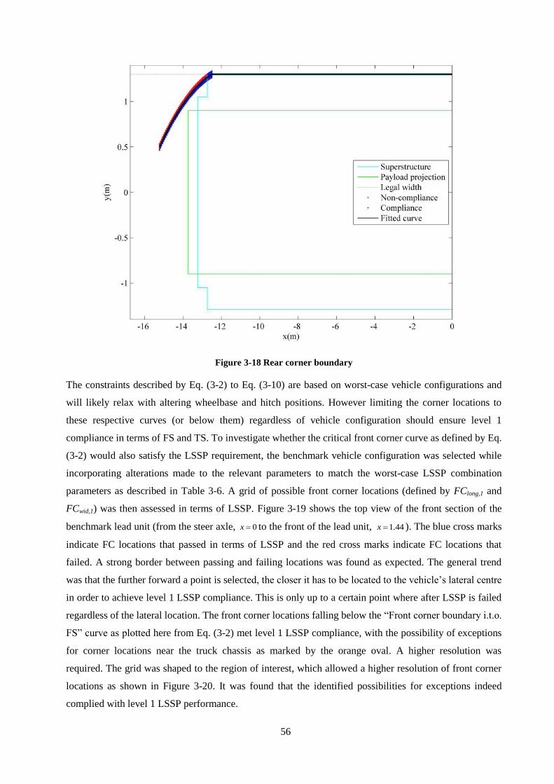
56
Figure 3-18 Rear corner boundary
The constraints described by Eq. (3-2) to Eq. (3-10) are based on worst-case vehicle configurations and
will likely relax with altering wheelbase and hitch positions. However limiting the corner locations to
these respective curves (or below them) regardless of vehicle configuration should ensure level 1
compliance in terms of FS and TS. To investigate whether the critical front corner curve as defined by Eq.
(3-2) would also satisfy the LSSP requirement, the benchmark vehicle configuration was selected while
incorporating alterations made to the relevant parameters to match the worst-case LSSP combination
parameters as described in Table 3-6. A grid of possible front corner locations (defined by FClong,1 and
FCwid,1) was then assessed in terms of LSSP. Figure 3-19 shows the top view of the front section of the
benchmark lead unit (from the steer axle, 0x to the front of the lead unit, 1.44x ). The blue cross marks
indicate FC locations that passed in terms of LSSP and the red cross marks indicate FC locations that
failed. A strong border between passing and failing locations was found as expected. The general trend
was that the further forward a point is selected, the closer it has to be located to the vehicle’s lateral centre
in order to achieve level 1 LSSP compliance. This is only up to a certain point where after LSSP is failed
regardless of the lateral location. The front corner locations falling below the “Front corner boundary i.t.o.
FS” curve as plotted here from Eq. (3-2) met level 1 LSSP compliance, with the possibility of exceptions
for corner locations near the truck chassis as marked by the orange oval. A higher resolution was
required. The grid was shaped to the region of interest, which allowed a higher resolution of front corner
locations as shown in Figure 3-20. It was found that the identified possibilities for exceptions indeed
complied with level 1 LSSP performance.

57
Figure 3-19 Grid search of critical FC locations in terms of LSSP
Figure 3-20 Shaped search of critical FC locations in terms of LSSP

58
Test runs: Using defined critical corners
The low-speed pro-forma bounds were again tested, this time placing all corners according to their
relevant critical boundary equations as per Eq. (3-4), Eq.(3-6) and Eq.(3-9). Three equally spaced
locations for each corner was assessed in combination with the remaining parameters as described in
Table 3-8 and incorporating the revised WB1 lower limit. Following this approach, a total of 4932 (11.9%
of total of 41472) combinations were found not to comply with the level 1 low-speed standards due to FS
and/or TS performance. The worst FS recorded was 0.713 m, only (1.9% over the allowed 0.7 m). The
worst TS performance was 0.326 m (8.7% over the allowed 0.3 m). Considering that Eq.(3-4), Eq.(3-6)
and Eq.(3-9) are based on a polynomial fitting that will inherently have a small error depending on the
resolution, it is understandable that some points on the defined line will not comply with the applicable
standard. The combination that resulted in the worst FS was re-assessed while reducing the FCwid,1 value
until it passed the FS requirement. It was found that the FCwid,1 value needed to be reduced by 0.04 m and
Eq. (3-3) and Eq. (3-4) needed to be altered to Eq. (3-11) and Eq. (3-12) respectively:
For:
0 :1.294x : 1.3y (3-11)
1.294 : 2.433x : 20.0647 0.4616 2.0257 0.02y x x (3-12)
Similarly, the combination that produced the worst TS (on the tractor) was re-assessed while reducing the
RCwid,1 value until it passed the TS requirement. It was found that the RCwid,1 value needed to be reduced
by 0.05 m and Eq. (3-6) and Eq. (3-7) needed to be altered to Eq. (3-13) and Eq. (3-14) respectively:
For:
11.792 : 9.276x : 20.0530 0.7987 1.5234 0.025y x x (3-13)
9.276 : 0x : 1.3y (3-14)
Similarly, the combination that produced the worst TS (on the trailer) was re-assessed while reducing the
RCwid,2 value until it passed the TS requirement. It was found that the RCwid,1 value needed to be reduced
by 0.06 m and Eq. (3-9) and Eq. (3-10) needed to be altered to Eq. (3-15) and Eq. (3-16) respectively:
For:
15.161: 12.22x : 20.0614 1.4092 6.7217 0.03y x x (3-15)
12.22 : 0x : 1.3y (3-16)
The test as described above was rerun using the updated corner definitions as given by Eq. (3-12), Eq.
(3-13), Eq. (3-15). The number of equally spaced locations for each corner was increased from three to
five to further check the boundaries. This resulted in 192000 potential designs that needed to be evaluated

59
which was computationally expensive requiring six days of computer processing. It was found that
190080 (99%) out of 192000 combinations complied with level 1 low-speed performance. The cases of
non-compliance (1%) were all due to TS failing to meet level 1 performance. The most severe non-
compliance was the combination that produced a TS of 0.3004 m, only 0.13% over the allowed limit.
This is an acceptable amount of non-compliance considering the limited accuracy of the LSMM as
described in section 3.1.1.
Practicality of proposed low-speed pro-forma
The proposed low-speed pro-forma has been shown to ensure level 1 compliance for low-speed PBS. It is
however important that the limits are lenient enough that a 23 m overall length (including payload) is still
achievable as per the RCC. The maximum potential vehicle length was calculated as follows:
Assuming a frontal projection width of 1.800 m (equal to that of the commercial car-carrier) the frontal
overhang can be calculated using Eq. (3-12) which gives a front overhang of 1.89 m as per Eq. (3-17).
The trailer’s rear overhang can similarly be calculated using Eq. (3-15) as per Eq. (3-18) which gives a
rear overhang (measured from the hitch point) of 14.1 m. Considering that the maximum allowable hitch
position, H1 (measured from the steer axle of the truck) is 8.025 m as per Table 3-8, the maximum length
of the combination (including payload projection) is thus the sum of these values, 24.0 m. This shows that
there is some room for design variations within the pro-forma design.
1.294 : 2.433x : 21.8
0.0647 0.4616 2.0257 0.022
x x (3-17)
15.161: 12.22x : 21.8
0.0614 1.4092 6.7217 0.032
x x (3-18)
To test the robustness of the pro-forma, a new 50/50 car-carrier concept design was obtained from the
commercial car-carrier manufacturer consisting of a Volvo FM62TT hauling the Macroporter MK3 as
shown in Figure 3-21.
Figure 3-21 Volvo FM62TT hauling the Macroporter MK3

60
Formal PBS assessment showed this design to comply with level 1 PBS. The design was subsequently
assessed using the pro-forma design as shown in Table 3-9. Here, six parameters failed in terms of the
low-speed pro-forma as shown in red. These included the front and rear corners, truck axle spacing, as
well as the two wheelbases. The current pro-forma design may thus be regarded as too strict for use in
practice. One could argue that the pro-forma limit range set for WB1 should have been designed to allow
for higher wheelbase values. However, according to Prem et al. [17] (as summarised in Table 1-3 and
confirmed in Figure 3-3), increasing the prime mover wheelbase has a significantly negative effect on
frontal swing performance. This would imply more strict limiting of the front corner which was already
not complying with the pro-forma limit as shown in red in Table 3-9. A similar situation exists in terms of
tail swing considering WB2 and the trailer’s rear corner failing to meet the pro-forma design.
Table 3-9 Assessing a new concept design using pro-forma design
Pro-forma limits Volvo FM 62TT +
Macroporter MK3
Parameter Min Max
T 2.3 2.542 2.494
WB1 5.690 6.185 6.2825
FClong,1 1.35
FCwid,1 *2.529 2.596
RClong,1 9.96
RCwid,1 *2.298 2.3
n1 1 2 2
d1 1.34 1.36 1.365
IEwid,1 2.550 2.6 2.55
H1 7.8 8.025 8.025
WB2 8.5 8.85 8.3
FClong,2 0 0 0
FCwid,2 0 0 0
RClong,2 12.585
RCwid,2 *2.52 2.58
n2 1 3 2
d2 1.34 1.6 1.5
IEwid,2 2.550 2.6 2.58
H2 0 0 0
*Calculated according to the relevant formulae as per Eq. (3-11) to Eq. (3-16).
As shown by the sensitivity analysis conducted earlier, WB1, WB2 and H1 have significant influence on the
low-speed standards. In order to have these parameters limited to a simple-to-enforce minimum and
maximum, the allowed projections had to be calculated at the worst-case WB1, WB2 and H1 for the
applicable standard to ensure compliance for all WB1, WB2 and H1 design variations. This resulted in
over-conservative projection limitations, compromising the practicality of the pro-forma design.

61
Customisable pro-forma design
An alternative approach was investigated which would allow the user of the pro-forma design to specify a
particular WB1, WB2 and H1 from which customised allowed projections could be predicted. To ensure a
practical solution, the vehicle parameters from five level 1 SASTRP PBS-approved 50/50-type car-
carriers were investigated. The individual parameter values were extracted from the relevant PBS report
and are summarised in Table 3-10. The vehicle parameter values shown in red would not have passed the
original pro-forma design and was incorporated into the new, customisable pro-forma design’s limits to
ensure a more practical solution.
Table 3-10 Vehicle parameters of five 50/50- type car-carriers
Parameter Commercial 50/50 Car-Carriers
Mercedes-Benz
Actros 2541+
Macroporter
MK3
Volvo FM 62TT
+ Macroporter
MK3
Volvo FM400 +
Lohr MHR 3.10
EHR 2.10
Mercedes-Benz
Actros 2541-54 +
Lohr MHR 3.30 AS
D1 2.03 XS
Scania P410 LB
6x2 MNA + Lohr
MHR EHR
T 2.351 2.494 2.494 2.1935 2.2245
WB1 6.075 6.2825 6.2825 6.075 6.175
FClong,1 1.94 1.89 1.86 1.84 1.852
FCwid,1
RClong,1 10.025 10.04 10.93 10.687
RCwid,1
n1 2 2 2 2 2
d1 1.35 1.365 1.365 1.35 1.35
IEwid,1 2.58 2.55 2.502 2.5
H1 7.825 8.025 8.465 8.08 8.37
WB2 8.5 8.3 7.97 8.275 7.97
FClong,2 0 0 0 0 0
FCwid,2 0 0 0 0 0
*RClong,2 13.7 13.585 13.175 13.48 13.072
*RCwid,2
n2 2 2 2 2 2
d2 1.5 1.5 1.36
IEwid,2 2.58 2.58 2.54 2.542
H2 0 0 0 0 0
The minimum and maximum parameter values for the customisable pro-forma were selected based on the
extremities shown in Table 3-10, while also incorporating additional practical recommendations made by
the experienced car-carrier manufacturer. These proposed limits are shown in Table 3-11. In order to
specify the projection permitted for level 1 low-speed PBS compliance, an accurate prediction of FS, TS
and LSSP is required based on each customised vehicle design. To achieve this, the LSMM was used to
evaluate, firstly, the frontal swing of 2000 randomly generated potential vehicle designs. The vehicle

62
designs were generated by assigning a randomly generated value to all the parameters indicated by “var”
within the respective minimum and maximum bounds as shown in the FS column, using a similar
approach as demonstrated earlier by Eq. (3-1). These parameters represent the customisable parameters
for FS. The remaining vehicle parameters in the FS column were selected as the minimum or maximum,
whichever had the most detrimental effect on frontal swing performance as previously determined by the
sensitivity analysis. Note that the values shaded grey do not influence the FS and were arbitrarily chosen
as that of the commercial car-carrier.
Table 3-11 Customisable pro-forma limits
Proposed limits Bounds for LSMM
Standard
Parameter Min Max FS LSSP TS (Truck) TS (Trailer)
T 2.1935 2.494 2.494 2.351 2.351 2.351
WB1 5.75 6.35 var var var var
FClong,1 0.5 1.94 var var 1.352 1.352
FCwid,1 1 2.5 var var 0.2596 2.596
RClong,1 8.35 11.93 10.025 10.025 var 6.45
RCwid,1 1 2.5 2.3 2.3 var 0.23
n1 2 2 2 2 2 2
d1 1.3 1.5 1.5 1.5 1.3 1.3
IEwid,1 2.5 2.6 var 2.6 var 2.58
H1 7.5 8.5 7.825 var 7.825 var
WB2 7.5 9.2 8.5 var 8.5 var
FClong,2 0 0 0 0
FCwid,2 0 0 0 0
RClong,2 11.2 14.7 12.735 12.735 8.6 var
RCwid,2 1 2.5 2.58 2.58 0.258 var
n2 2 2 2 2 2 2
d2 1.3 1.8 1.5 1.8 1.5 1.3
IEwid,2 2.5 2.6 2.58 2.6 2.58 var
H2 0 0 0 0
Linear multivariate polynomial regression was performed using an algorithm developed by Cecen [27].
The algorithm predicts how the frontal swing performance change as result of changes to the four variable
parameters, indicated by “var” in the FS column in Table 3-11. The algorithm was allowed to “learn”
from 50% of the 2000 vehicle designs and their respective frontal swing performance. Based on the
regression, a relationship was found as shown in Eq. (3-19) and Table 3-12. The remaining designs and
respective frontal swing performance were then used to test the accuracy of the prediction. The maximum
absolute error was 0.18% and and the average absolute error was 0.02%. These errors were regarded
acceptable considering the accuracy of the LSMM.

63
1 4
2 3
3 3* 4
4 2
5 2 * 4
6 2 * 3
7 1
.8 1* 4
9 1* 3
10 1* 2
11 1.0
12 1^ 2
13 2 ^ 2
14 3 ^ 2
15 4 ^ 2
C x
C x
C x x
C x
C x x
C x x
C x
FSC x x
C x x
C x x
C
C x
C x
C x
C x
(3-19)
Table 3-12 Parameter description for FS prediction
Parameter Value/Description
1C -0.4948000
2C 0.5298000
3C 0.0002533
4C 0.1981000
5C 0.0004618
6C -0.0152800
7C 0.1147000
8C -0.0006721
9C -0.0166900
10C 0.0513800
11C -0.3372000
12C -0.0050510
13C 0.0236600
14C 0.0027080
15C -0.0004205
1x WB1
2x FClong,1
3x FCwid,1
4x IEwid,1
The same approach was used for developing a conservative prediction of LSSP as shown in Eq. (3-20)
and Table 3-13, but here five parameters were selected to have varying values, indicated by “var” in the
LSSP column in Table 3-11. The maximum absolute error was 0.02% and and the average absolute error
was 0.002%. These errors were regarded acceptable considering the accuracy of the LSMM.

64
1 5
2 4
3 4 * 5
4 3
5 3* 5
6 3* 4
7 2
8 2 * 5
9 2 * 4
10 2 * 3
.11 1
12 1* 5
13 1* 4
14 1* 3
15 1* 2
16 1
17 1^ 2
18 2 ^ 2
19 3 ^ 2
20 4 ^ 2
21
C x
C x
C x x
C x
C x x
C x x
C x
C x x
C x x
C x x
C x
C x x
C x x
C x x
C x x
C
C x
C x
C x
C x
C
5 ^ 2
LSSP
x
(3-20)
Table 3-13 Parameter description for LSSP prediction
Parameter Value/Description
1C -0.0492100
2C 0.3416000
3C 0.0032430
4C 0.5047000
5C -0.0004602
6C 0.0003142
7C 0.2469000
8C 0.0016760
9C -0.0011290
10C -0.0124300
11C 0.3526000
12C 0.0413600
13C -0.0171000
14C -0.0098050
15C 0.0345300
16C -0.0785800
17C -0.0062910
18C 0.0219700
19C 0.0017660
20C 0.0123300
21C -0.0197700
1x WB1
2x FClong,1
3x FCwid,1
4x WB2
5x H1

65
The same approach was used for developing a conservative prediction of TS of the truck as shown in Eq.
(3-21) and Table 3-14, but here four parameters were selected to have varying values, indicated by “var”
in the TS (Truck) column in Table 3-11. The maximum absolute error was 1.0% and the average absolute
error was 0.069%. These errors were regarded acceptable considering the accuracy of the LSMM.
1 4
2 3
3 3 4
4 2
5 2 * 4
6 2 * 3
7 1
.8 1* 4
9 1* 3
10 1* 2
11 1.0
12 1^ 2
13 2 ^ 2
14 3 ^ 2
15 4 ^ 2
C x
C x
C x x
C x
C x x
C x x
C x
TS truckC x x
C x x
C x x
C
C x
C x
C x
C x
(3-21)
Table 3-14 Parameter description for TS (truck) prediction
Parameter Value/Description
1C -0.5241000
2C -0.0221500
3C 0.0030720
4C 0.5212000
5C 0.0000974
6C 0.0153200
7C 0.0040830
8C 0.0001888
9C -0.0912300
10C -0.0129300
11C 0.0340700
12C 0.0395400
13C 0.0012850
14C 0.0539800
15C 0.0006801
1x RClong,1
2x RCwid,1
3x WB1
4x IEwid,1
The same approach was used for developing a conservative prediction of TS of the trailer as shown in Eq.
(3-22) and Table 3-15, but here six parameters were selected to have varying values, indicated by “var”

66
in the TS (Trailer) column in Table 3-11. The maximum absolute error was 2.7% and and the average
absolute error was 0.23%. These errors were regarded acceptable considering the accuracy of the LSMM.
1 6
2 5
3 5* 6
4 4
5 4 * 6
6 4 * 5
7 3
8 3* 6
9 3* 5
10
11
12
13
14.
15
16
17
18
19
20
21
22
23
24
25
26
27
28
C x
C x
C x x
C x
C x x
C x x
C x
C x x
C x x
C x
C
C
C
C
C
C
C
C
C
C
C
C
C
C
C
C
C
C
3* 4
2
2 * 6
2 * 5
2 * 4
2 * 3
1
1* 6
1* 5
1* 4
1* 3
1* 2
1
1^ 2
2 ^ 2
3 ^ 2
4 ^ 2
5 ^ 2
6 ^ 2
x
x
x x
x x
x xTS trailer
x x
x
x x
x x
x x
x x
x x
x
x
x
x
x
x
(3-22)
Table 3-15 Parameter description for TS (trailer) prediction
Parameter Value/Description
1C -0.007489
2C 0.02337
3C -0.04914
4C -0.7791
5C -0.00927
6C -0.02116
7C 0.02756
8C -0.00888
9C 0.02072
10C -0.009909
11C 0.5652
12C -0.004087
13C -0.002367
14C 0.03594

67
15C 0.02263
16C -0.03022
17C 0.004978
18C -0.01521
19C 0.009211
20C -0.0872
21C -0.02283
22C 0.2575
23C 0.04017
24C -0.0006539
25C 0.04803
26C 0.07101
27C 0.03056
28C 0.02553
1x RClong,2
2x RCwid,2
3x WB2
4x IEwid,2
5x WB1
6x H1
An assessment tool was developed in Microsoft Excel using Visual Basic as shown in Figure 3-22. The
tool accepts five vehicle-specific parameters covering all “var” parameters from Table 3-11. Using Eq.
(3-19) to Eq. (3-22), the tool calculates the allowed projections for level 1 low-speed PBS compliance and
superimposes these limits onto a top-view drawing of the proposed vehicle as shown in Figure 3-23. If all
corners of the vehicle and payload projection falls within the boundaries indicated in red, the vehicle is
deemed to comply with level 1 FS and TS requirements. LSSP is also predicted, notifying the user when
level 1 LSSP compliance is not achieved. Furthermore, the output gives a simple visual indication to the
vehicle designer of where critical areas/non-critical areas are without the vehicle designer being required
any understanding of PBS.
Figure 3-22 Assessment tool: low-speed PBS (input)

68
Figure 3-23 Assessment tool: low-speed PBS (output)
All five of the the commercial car-carriers from Table 3-10 were assessed using the Excel tool and found
to pass the low-speed pro-forma as shown below. Note that in some cases, the top-view drawing was
rotated in the interest of sign convention.
Figure 3-24 Assessment of the Mercedes-Benz Actros 2541+ Macroporter MK3
Figure 3-25 Assessment of the Volvo FM 62TT + Macroporter MK3
Figure 3-26 Assessment of the Volvo FM400 + Lohr MHR 3.10 EHR 2.10

69
Figure 3-27 Assessment of the Mercedes-Benz Actros 2541-54 + Lohr MHR 3.30 AS D1 2.03 XS
Figure 3-28 Assessment of the Scania P410 LB 6x2 MNA + Lohr MHR EHR
Steer tyre friction demand
MoD and DoM are not applicable to the 50/50 car-carrier type as the trailers have no front overhang.
Based on Table 1-2, the only remaining low-speed PBS standard to consider is steer tyre friction demand
(STFD). The commercial car-carrier PBS assessment showed a STFD performance of only 27%. This is
well below the maximum allowed limit of 80%. According the the Australian PBS rules [4], STFD is
typically only a concern for multi-combination vehicles with tri-axle drive combinations that have a
widely spread drive axle layout. It is further specified that STFD is generally not an issue for prime
movers with single-axle or tandem-axle drive axle configurations. Following Table 3-11 our customisable
pro-forma design only allows for tandem-axle drive systems (n1 = 2) and as such, vehicles complying
with the pro-forma requirements will inherently comply with STFD requirements.
3.2. Remaining PBS
The remaining PBS standards are shown in Table 3-16, with the low-speed PBS standards that were
covered in the previous section being blocked out in grey.

70
Table 3-16 PBS standards to consider
Manoeuvre Safety Standard Description
Accelerate from rest on an incline 1. Startability (St) Maximum upgrade on which the vehicle
can start from rest.
Maintain speed on an incline
2.a. Gradeability A (GrA) Maximum upgrade on which the vehicle
can maintain forward motion.
2.b. Gradeability B (GrB) Maximum speed that the vehicle can
maintain on a 1% upgrade
Cover 100 m from rest 3. Acceleration capability (AC) Intersection/rail crossing clearance times.
Low-speed 90° turn
4. Low-speed swept path (LSSP) “Corner cutting” of long vehicles.
5. Frontal swing (FS) Swing-out of the vehicle’s front corner.
5a. Maximum of Difference (MoD) The difference in frontal swing-out of
adjacent vehicle units where one of the
units is a semitrailer. 5b. Difference of Maxima (DoM)
6. Tail swing (TS) Swing-out of the vehicle’s rear corner.
7. Steer-tyre friction demand (STFD) The maximum friction utilised by the steer-
tyres.
Straight road of specified
roughness and cross-slope
8. Tracking ability on a straight path
(TASP)
Total road width utilised by the vehicle as it
responds to the uneven road at speed.
Constant radius turn (increasing
speed) or tilt-table testing 9. Static rollover threshold (SRT)
The maximum steady lateral acceleration a
vehicle can withstand before rolling.
Single lane-change
10. Rearward amplification (RA) “Whipping” effect of trailing units.
11. High-speed transient offtracking
(HSTO) “Overshoot” of the rearmost trailing unit.
Pulse steer input 12. Yaw damping coefficient (YDC) The rate at which yaw oscillations settle.
Before attempting to develop a pro-forma for each of the remaining standards, we consider the PBS
performance of the five commercial car-carriers as described earlier in Table 3-10 to identify the critical
standards for 50/50-type car-carriers.
3.2.1. Typical PBS performance of 50/50-type car-carriers
The PBS performance of five commercial 50/50-type car-carriers are shown in Table 3-17. The top half
of this table indicates the PBS performance while the bottom half shows the performance achieved as a
fraction of the relevant level 1 limit. Naturally, for standards where the performance is required to be less
than a certain value, such as acceleration capability, the fraction was calculated as the performance
divided by the required performance. For the standards where the performance is required to be greater
than a certain value, such as SRT, the inverse fraction was calculated, that is, the limit (0.35g in this case)
divided by the relevant performance. Using the latter approach slightly skews the results as the
benchmark/denominator is not consistent, but gives a useful indication of what the critical standards are
for 50/50-type car-carriers. Cases where the performance is close to the limit (~=100 %) are shaded red
and those far from the limits (<<100 %) are shaded blue.

71
Table 3-17 PBS performance of five commercial 50/50 car-carriers
The performance of the combinations in terms of startability, gradeability A and acceleration capability is
borderline for a number of combinations as shown in Table 3-17. It is thus important that these standards
are further investigated to specify a rule or model to ensure compliance for the pro-forma design.
Gradeability B was found not to be a concern, especially considering the revised requirements of the
SASTRP. The TASP performance was borderline but the SASTRP has previously relaxed the TASP
requirements on a case-by-case basis as South African road widths are wider than Australian road widths
and can thus accommodate poorer TASP performance. When operating within the pro-forma design,
LSSP, FS and TS have been accounted for. FS, which is the most critical PBS standard based on Table
3-17, will thus inherently be governed. In coherence with the NTC’s arguments, STFD was found to be
non-critical for the five combinations. The SRT performance of four of the five combinations were close
to the limit. SRT will thus be investigated further especially considering the significance of this standard
as shown in the literature review. The RA performance of all five car-carriers was far from the relevant
limit. This is typical for this vehicle configuration and low number of articulation points. HSTO and YD
were far from their respective limits.
We now consider the standards that were identified as borderline and not regulated by the low-speed pro-
forma with the aim of finding a simple method to insure compliance.
13 13 15 13 24 ≥ 12%
Gradeability A (Maintain motion) (%) 18 15 16 16 25 ≥ 15%
Gradeability B (Maintain speed) (km/h) 88 95 89 89 89 ≥ 70 km/h
Acceleration Capability (s) 16.5 16.0 18.1 16.6 18.9 ≤ 20.0 s
Tracking Ability on a Straight Path (m) 2.8 2.8 2.7 2.8 2.7 ≤ 2.9 m
7.0 7.1 6.7 6.7 6.7 ≤ 7.4 m
0.7 0.7 0.7 0.7 0.7 ≤ 0.7 m
0.25 0.24 0.26 0.26 0.18 ≤ 0.30 m
Steer-Tyre Friction Demand (%) 24 35 29 23 34 ≤ 80%
Static Rollover Threshold (g) 0.37 0.38 0.45 0.38 0.37 ≥ 0.35·g
Rearward Amplification 1.30 1.83 1.68 1.10 1.94 ≤ 5.7·SRT_rrcu*
High-Speed Transient Offtracking (m) 0.4 0.5 0.5 0.5 0.5 ≤ 0.6 m
Yaw Damping Coefficient @ 80 km/h 0.28 0.30 0.36 0.29 0.19 ≥ 0.15
* 5.7·SRT_rrcu (g) 2.11 2.17 2.57 2.51 2.68
92% 92% 80% 92% 50% ≥ 12%
Gradeability A (Maintain motion) (%) 83% 97% 97% 94% 60% ≥ 15%
Gradeability B (Maintain speed) (km/h) 80% 74% 79% 79% 79% ≥ 70 km/h
Acceleration Capability (s) 83% 80% 91% 83% 95% ≤ 20.0 s
Tracking Ability on a Straight Path (m) 96% 97% 93% 97% 93% ≤ 2.9 m
95% 96% 91% 91% 91% ≤ 7.4 m
100% 100% 100% 100% 100% ≤ 0.7 m
83% 80% 87% 87% 60% ≤ 0.30 m
Steer-Tyre Friction Demand (%) 30% 44% 36% 29% 43% ≤ 80%
Static Rollover Threshold (g) 95% 92% 78% 92% 95% ≥ 0.35·g
Rearward Amplification 62% 84% 65% 44% 72% ≤ 5.7·SRT_rrcu*
High-Speed Transient Offtracking (m) 67% 83% 85% 83% 82% ≤ 0.6 m
Yaw Damping Coefficient @ 80 km/h 54% 50% 42% 52% 79% ≥ 0.15
Tail Swing (m)
Low Speed Swept Path (m)
Frontal Swing (m)
Startability (%)
Tail Swing (m)
Low Speed Swept Path (m)
Frontal Swing (m)
Required
performance
Level 1
Startability (%)
Performance relative to level 1 limit
Mercedes Benz
Actros 2541 +
Macroporter
MK3
Volvo FM 62TT
+ Macroporter
MK3
Volvo FM400 +
Lohr MHR 3.10
EHR 2.10
Mercedes Benz
Actros 2541-54 +
Lohr MHR 3.30
AS D1 2.03 XS
Scania P410
LB 6x2 MNA
+ Lohr MHR
EHR

72
3.2.2. Startability, gradeability A and acceleration capability
In South Africa, engine power is governed by the NRTA’s strict power to weight ratio regulations [7].
Subsequently, the general trend in the PBS demonstration project thus far has been that startability,
gradeability A, and acceleration capability performance are typically limited by traction, rather than by
engine power. This is particularly applicable to 6x2 car-carrier trucks as the load on the drive axle is low.
Ensuring an acceptable drive axle load is thus the main priority when attempting to ensure acceptable
startability, gradeability A and acceleration capability performance.
A simple, effective method to ensure that sufficient drive axle load is achieved is to specify a minimum
drive axle load per ton GCM. To specify such a value for 50/50-type car-carriers, we assessed a worst-
case hypothetical design at 100 kg drive axle load increments to find the minimum required drive axle
load allowing level 1 startability, gradeability A, and acceleration capability performance to be achieved.
In the light of hypothesising a worst-case design, the GCMs of all five commercial car-carriers were
considered. The combination with the highest GCM was the Mercedes Benz Actros 2541-54 + Lohr
MHR 3.30 AS D1 2.03 XS, with a GCM of 43 300 kg. This was conservatively rounded up to 44 000 kg
for the hypothetical worst-case. The driveline data of the Volvo FM 62TT was assumed to be
representative. A worst case frontal area was assumed as 4.6 m x 2.6 m, the maximum allowed height and
width based on NRTA [7] and RCC [11].
The results are shown in Figure 3-29 to Figure 3-31. The minimum required drive axle loads based on
startability, gradeability A, and acceleration capability were 7 340 kg, 8480 kg and 4200 kg respectively.
The critical standard is gradeability A, requiring the highest drive axle load, 8480 kg. As a fraction of
GCM (44 000kg) this means that 19.3% (or more) of the total GCM is required to be loaded onto the
drive axle to ensure compliance.

73
Figure 3-29 Startability for various drive axle loads
Figure 3-30 Gradeability A for various drive axle loads

74
Figure 3-31 Acceleration capability for various drive axle loads
3.2.3. Static rollover threshold
In this section we evaluate the accuracy of the respective SRT prediction tools that have been identified in
the literature review (section 1.4.4), specifically for 50/50-type car-carriers as per Table 3-17. We
compare the SRT results obtained using each of the identified SRT tools with that of TruckSim®, with the
aim of identifying an acceptable tool to be used in conjunction with the pro-forma design to ensure
overall PBS compliance.
It is important to note that the NTC rules dictate that SRT be evaluated based on the complete hitched-up
vehicle combination, whereas using any of the identified tools, the SRT of only one single vehicle unit
can be evaluated at a time. The NTC further defines the point of roll instability as when the vertical load
on all of the non-steering tyres on the lightly loaded side of the combination have reduced to zero or when
the roll angle of any unit exceeds 30°. The identified tools generally defines instability when the load on
all tyres on the lightly loaded side of the vehicle unit have reduced to zero. Generally, 50/50-type car-
carrier trailers are hauled by pintle hitches with negligible roll-coupling. It is therefore expected that the
SRT performance of the worst-performing vehicle unit will correlate well with the overall combination
performance. The SRT tools were all programmed using Matlab® and the payload and suspension data

75
were sourced from the CSIR’s TruckSim® database as well as the relevant PBS reports as approved by the
SASTRP.
Results
Table 3-18 compares the SRT performance of various 50/50-type car-carriers as calculated using different
SRT prediction tools. For all the combinations, the trucks (as assessed using TruckSim®) were the worst-
performing vehicle units and their results correlated well with the results of the respective “Full
Combination”, also assessed using TruckSim®. Assessing the trucks using the methods of Gillespie [16],
Elischer & Prem [23], NZLTR “Case1” and NZLTR “Case2” required some assumptions to be made to
arrive at an effective suspension i.e. combining the front and rear suspension of the truck. The axle track
width, for example, was taken as the average of that of the front and rear suspensions, weighted by the
axle group load. Similar assumptions were made for spring track and roll centre heights. Stiffness features
were summed as these function in parallel. For NZLTR “Case3”, the front and rear suspension
characteristics are required to be specified separately, however again the concept of averaging was
applied in combining the drive and tag axles where non-identical. As expected, when compared to the
TruckSim® vehicle unit results as a baseline, the method of Gillespie [16] did not provide accurate results,
with an average absolute error of 40.5% for trucks and 18.5% for trailers. The method of Elischer &
Prem [23] provided more accurate results, especially considering the simplicity of the model with an
average absolute error of 7.4% for trucks and 11.4% for trailers. With the truck assessments, NZLTR
“Case1” proved to be less accurate than Elischer & Prem’s [23] method, with an absolute average error of
14.5%. NZLTR “Case2” was only applicable to the third truck, the Volvo FM400, which showed a 1.15%
error. The remainder of the trucks experienced wheel lift-off before lash could occur and was thus not
assessed using NZLTR “Case2”. The reason for this is the high auxiliary roll stiffness of the respective
trucks’ averaged suspensions. When using NZLTR “Case3”, the individual axle groups characteristics
were incorporated allowing an improved accuracy of 4.66%. No NZLTR “Case3” solution was found for
the two Volvo trucks. With the trailer assessments, the NZLTR “Case1” provided excellent accuracy with
an average absolute error of 0.82%. Here lash was also not achieved due to the high auxiliary roll
stiffness of the trailer axles. The methods of the NZLTR for predicting SRT was found to provide the best
correlation with TruckSim® results. This is likely due to the fact that the NZLTR approach incorporates
customised suspension characteristics, such as spring stiffness, auxiliary roll stiffness, tyres stiffness and
lash, allowing for improved prediction accuracy.

76
Table 3-18 SRT performance using various predictor tools
0.375 0.387 0.446 0.391 0.369
0.375 0.384 0.428 0.393 0.363
0.528 0.542 0.564 0.552 0.538
0.397 0.405 0.430 0.427 0.422
0.418 0.448 0.436 0.443 0.470
N/A N/A 0.432 N/A N/A
0.397 0.412 0.352
0.439 0.446 0.484 0.468 0.475
0.504 0.511 0.585 0.570 0.572
0.373 0.376 0.440 0.434 0.428
0.446 0.453 0.482 0.468 0.472
Average
absolute
error
Maximum
absolute
error
Gillespie 40.9% 41.2% 31.8% 40.6% 48.1% 40.5% 48.1%
Elischer & Prem 6.0% 5.4% 0.7% 8.6% 16.2% 7.4% 16.2%
NZLTR “Case 1” 11.4% 16.7% 2.0% 12.9% 29.3% 14.5% 29.3%
NZLTR “Case 2” N/A N/A 1.1% N/A N/A 1.1% 1.1%
NZLTR “Case 3” 6.0% N/A N/A 5.0% -3.0% 4.7% 6.0%
Gillespie 14.8% 14.5% 20.9% 21.7% 20.4% 18.5% 21.7%
Elischer & Prem -15.1% -15.8% -9.0% -7.3% -9.9% 11.4% 15.8%
NZLTR “Case 1” 1.7% 1.4% -0.4% 0.0% -0.6% 0.8% 1.7%
TruckSim
NZLTR “Case 3”
Gillespie
Elischer & Prem
NZLTR “Case 1”
SRT Model
Mercedes Benz
Actros 2541 +
Macroporter MK3
Volvo FM 62TT +
Macroporter
MK3
Volvo FM400 +
Lohr MHR 3.10
EHR 2.10
TruckSim (Full Combination)
Truck
Mercedes Benz
Actros 2541-54 +
Lohr MHR 3.30 AS
D1 2.03 XS
Scania P410 LB
6x2 MNA +
Lohr MHR
EHR
Truck
Trailer
TruckSim
Gillespie (Averaged)
Elischer & Prem (Averaged)
NZLTR “Case 1” (Averaged)
NZLTR “Case 2” (Averaged)
Trailer
Percentage error w.r.t vehicle unit's TruckSim SRT performance

77
4. CONCLUSION
A pro-forma approach has been developed for assessing 50/50-type car-carrier designs in terms of
compliance with the South African PBS pilot project requirements. All the relevant PBS were considered
and simplified means of assessing the critical standards were established. The low-speed PBS were
considered and a customisable low-speed pro-forma design was developed by empirically deriving
equations for the frontal swing, tail swing and low speed swept path standards, with a maximum absolute
error of 2.7%. These equations were incorporated into a simplified tool for assessing the low-speed PBS
compliance of car-carriers using a top-view drawing of the design. The minimum drive axle load required
was determined as 19.3% of the GCM to ensure that the vehicle passes startability, gradeability A and
acceleration capability. It was determined that the SRT performance can accurately be predicted by means
of the NZLTR method, with a maximum absolute error of 6% for the truck and 1.7% for the trailer.
The pro-forma approach offers a cost-effective and sustainable alternative to conventional TruckSim®
PBS assessments. The study is limited to 50/50-type car-carriers, however the methodology developed
will be used to construct assessment frameworks for short-long and tractor-and-semitrailer car-carrier
combinations as well as heavy combinations in other industries. The pro-forma will have a significantly
positive impact on the South African PBS pilot project by allowing for the efficient and sustainable PBS
assessment of future 50/50-type car-carrier combinations.

78
5. RECOMMENDATIONS FOR FURTHER WORK
The NZLTR method for calculating SRT specifies various default suspension parameters such as typical
spring stiffness, suspension track width, composite roll stiffness, axle lash and roll centre height for
generic steer, steel and air suspensions. For our validation, the exact values of these properties were
sourced from TruckSim® and the relevant PBS reports. As this information is time-consuming to gather
from OEMs, it is recommended that further investigation is done to assess the impact of using the generic
NZLTR suspension characteristics when assessing SRT for 50/50-type car-carriers. If these generic
characteristics provide acceptable results, it would streamline the assessment process significantly.

79
REFERENCES
[1] C. C. De Saxe, “Performance-Based Standards for South African Car-Carriers,” MSc disseration,
University of the Witwatersrand, Johannesburg, 2012.
[2] OECD Publishing, “Moving Freight with Better Trucks: Improving Safety, Productivity and
Sustainability,” 2011.
[3] Council for Scientific and Industrial Research, “10th Annual State of Logistics Survey for South
Africa,” Pretoria, 2013.
[4] National Transport Commission, “Performance Based Standards Scheme – The Standards and
Vehicle Assessment Rules,” Melbourne, 2008.
[5] Smart Truck Steering Committee and CSIR Built Environment, “Smart Truck Programme: Rules
for the Development and Operation of Smart Trucks as Part of the Performance-Based Standards
Research Programme in South Africa,” Pretoria, 2012.
[6] P. A. Nordengen, “The Development and Evaluation of a Performance-Based Standards Approach
for Regulating the Use of Heavy Vehicles in South Africa,” PhD thesis, University of KwaZulu-
Natal, Durban, 2014.
[7] Department of Roads and Transport, “National Road Traffic Act No. 93,” Republic of South
Africa, 1996.
[8] H. L. Theyse, M. De Beer, and F. C. Rust, “Overview of the South African Mechanistic Pavement
Design Analysis Method,” in Proceedings of the 75th Annual Transportation Research Board
Meeting, Washington D.C., pp. 96-137, 1996.
[9] “Advantia Transport Consulting.” [Online]. Available: http://www.advantia.com.au/. [Accessed:
25-Nov-2015].
[10] “ARRB Group: Advisor on Roads Transport.” [Online]. Available:
https://www.arrb.com.au/home.aspx. [Accessed: 25-Nov-2015].
[11] Abnormal Load Technical Committee, “Roadmap for the Regulation of Car Carriers in South
Africa,” 2014.
80
[12] NZ Transport Agency, “High Productivity Motor Vehicle Permits: Pro-Forma Designs,” 2014.
[Online]. Available: http://www.nzta.govt.nz/vehicle/your/hpmv/proforma.html#application.
[Accessed: 04-Aug-2014].
[13] Department of Transport, “PBS Blueprints and Resources,” 2014. [Online]. Available:
https://www.nhvr.gov.au/road-access/performance-based-standards/pbs-blueprints-and-resources.
[Accessed: 04-Aug-2014].
[14] J. De Pont, “The Development of Pro-Forma Over-Dimension Vehicle Parameters,” TERNZ,
2010.
[15] P. Fancher and C. Winkler, “Directional Performance Issues in Evaluation and Design of
Articulated Heavy Vehicles,” Vehicle System Dynamics., vol. 45, pp. 607–647, 2007.
[16] T. D. Gillespie, “Fundamentals of Vehicle Dynamics,” Society of Automotive Engineers, 1992.
[17] H. Prem, J. De Pont, B. Pearson, and J. McLean, “Performance Characteristics of the Australian
Heavy Vehicle Fleet,” Melbourne, 2002.
[18] J. De Pont, P. Baas, D. Hutchinson, and D. Kalasih, “Including Performance Measures in
Dimensions and Mass Regulations,” in Proceedings of the 7th International Symposium on Heavy
Vehicle Weights and Dimensions, pp. 349–358, 2002.
[19] C. Winkler, “Rollover of Heavy Commercial Vehicles,” UMTRI Research Review, vol. 31, no. 4,
pp. 1–20, 2000.
[20] T. Mueller, J. De Pont, and P. Baas, “Heavy Vehicle Stability Versus Crash Rates,” 1999.
[21] NZ Transport Agency, “Vehicle Classes,” 2015. [Online]. Available:
https://www.nzta.govt.nz/vehicles/vehicle-types/vehicle-classes-and-standards/vehicle-
classes/#NC.
[22] New Zealand Government, “Land Transport Rule : Vehicle Dimensions and Mass 2002,” New
Zealand, 2014.
[23] M. Elischer and H. Prem, “Stability of Over-Height Low-Density Freight Vehicles and Its
Prediction,” in Proceedings of the 5th International Symposium on Heavy Vehicle Weights and
Dimensions, pp. 147–160, 1998.

81
[24] R. Benade, R. Berman, and F. Kienhöfer, “PBS Assessment: Macroporter Truck-and-Trailer Car-
Carrier,” Technical Report, Pretoria, 2014.
[25] G. J. Heydinger, R. A. Bixel, W. R. Garrott, M. Pyne, J. G. Howe, and D. A. Guenther, “Measured
Vehicle Inertial Parameters-NHTSA’s Data Through November 1998,” SAE Progress in
Technology, vol. 101, pp. 531–554, Mar. 2004.
[26] R. Benade, F. Kienhöfer, R. Berman, and P. A. Nordengen, “A Pro-Forma Design for Car-
Carriers : Low-Speed Performance-Based Standards,” in Proceedings of the 34th South African
Transport Conference, pp. 253–265, 2015.
[27] A. Cecen, “Multivariate Polynomial Regression,” Mathworks, 2015.

82
APPENDIX A
The modelling of the commercial car-carrier is described in more detail in this section.
Suspension characteristics A.1.
The information presented here represents the final characteristics as inputted into TruckSim®. It is worth
noting that several lever calculations were performed based on the suspension geometry arriving at the
following final effective characteristics:
A.1.1. Force/displacement characteristics
The different airbags fitted to the different axles resulted in the following force/displacement
characteristics:
Figure A - 1 Truck drive axle (per side)

83
Figure A - 2 Truck tag axle (per side)
Figure A - 3 Trailer axle (per axle, per side)

84
A.1.2. Force/velocity characteristics
The different dampers fitted to the different axles resulted in the following force/velocity characteristics:
Figure A - 4 Truck steer axle (per side)
Figure A - 5 Truck drive axle (per side)
Rebound Bump
Rebound Bump

85
Figure A - 6 Truck tag axle (per side)
Figure A - 7 Trailer axle (per axle, per side)
Rebound Bump
Rebound Bump

86
Driveline characteristics A.2.
The following engine characteristics were obtained from the OEM:
Table A - 1 Engine torque output
Engine
speed
(rpm)
Torque
developed
(Nm)
1050 1970
1100 2000
1150 2000
1200 1990
1300 1960
1400 1930
1500 1870
1600 1770
1700 1680
1800 1585
1900 1450
1980 1300
The following gear ratios and respective efficiencies were obtained from the OEM. The differential ratio
was specified as 2.533:1 with an efficiency of 97%.
Table A - 2 Gearbox efficiency
Gear Ratio Efficiency
1 14.93 96
2 11.67 96
3 9.02 96
4 7.06 96
5 5.63 96
6 4.4 96
7 3.39 96
8 2.65 96
9 2.05 96
10 1.6 96
11 1.28 96
12 1 98