A primer to scaffolded DNA origami -...
31
Nature Methods A primer to scaffolded DNA origami Carlos Ernesto Castro, Fabian Kilchherr, Do-Nyun Kim, Enrique Lin Shiao, Tobias Wauer, Philipp Wortmann, Mark Bathe & Hendrik Dietz Supplementary Figure 1 Scaffold / staple layout for the straight ‘robot’ object. Supplementary Figure 2 Scaffold / staple layout for the 18 helix bundle. Supplementary Figure 3 Scaffold / staple layout for the 24 helix bundle. Supplementary Figure 4 Scaffold / staple layout for the 32 helix bundle. Supplementary Figure 5 Scaffold / staple layout for a tetrameric 60 helix bundle. Supplementary Protocol 1 Step-by-step scaffold production from phage DNA. Supplementary Protocol 2 Setting up folding reactions. Supplementary Protocol 3 Agarose Gel Electrophoresis (EtBr) with DNA origami objects. Supplementary Protocol 4 Negative-Staining for Transmission Electron Microscopy. Supplementary Protocol 5 Imaging DNA origami shapes with atomic force microscopy. Supplementary Note 1 Understanding caDNAno diagrams and source files. Supplementary Note 2 Computer-aided engineering for DNA origami: ‘CanDo’. Supplementary Methods Nature Methods: doi.10.1038/nmeth.1570
-
Upload
vuongtuong -
Category
Documents
-
view
216 -
download
0
Transcript of A primer to scaffolded DNA origami -...
Nature Methods
A primer to scaffolded DNA origami Carlos Ernesto Castro, Fabian Kilchherr, Do-Nyun Kim, Enrique Lin Shiao, Tobias Wauer, Philipp Wortmann, Mark Bathe & Hendrik Dietz Supplementary Figure 1 Scaffold / staple layout for the straight ‘robot’ object.
Supplementary Figure 2 Scaffold / staple layout for the 18 helix bundle.
Supplementary Figure 3 Scaffold / staple layout for the 24 helix bundle.
Supplementary Figure 4 Scaffold / staple layout for the 32 helix bundle.
Supplementary Figure 5 Scaffold / staple layout for a tetrameric 60 helix bundle.
Supplementary Protocol 1 Step-by-step scaffold production from phage DNA.
Supplementary Protocol 2 Setting up folding reactions.
Supplementary Protocol 3 Agarose Gel Electrophoresis (EtBr) with DNA origami objects.
Supplementary Protocol 4 Negative-Staining for Transmission Electron Microscopy.
Supplementary Protocol 5 Imaging DNA origami shapes with atomic force microscopy.
Supplementary Note 1 Understanding caDNAno diagrams and source files.
Supplementary Note 2 Computer-aided engineering for DNA origami: ‘CanDo’.
Supplementary Methods
Nature Methods: doi.10.1038/nmeth.1570
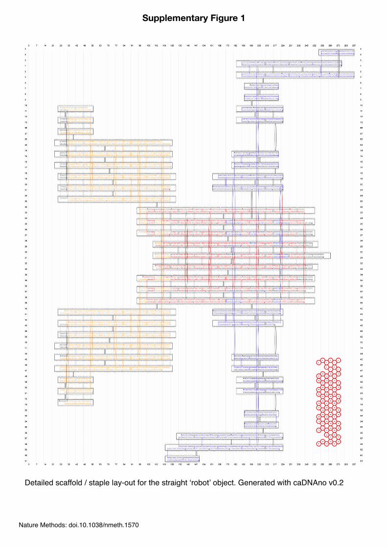
Supplementary Figure 1
Detailed scaffold / staple lay-out for the straight ʻrobotʼ object. Generated with caDNAno v0.2
Nature Methods: doi.10.1038/nmeth.1570
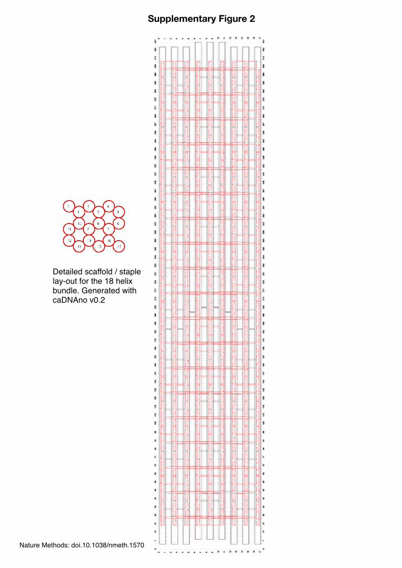
Detailed scaffold / staple lay-out for the 18 helix bundle. Generated with caDNAno v0.2
Supplementary Figure 2
Nature Methods: doi.10.1038/nmeth.1570
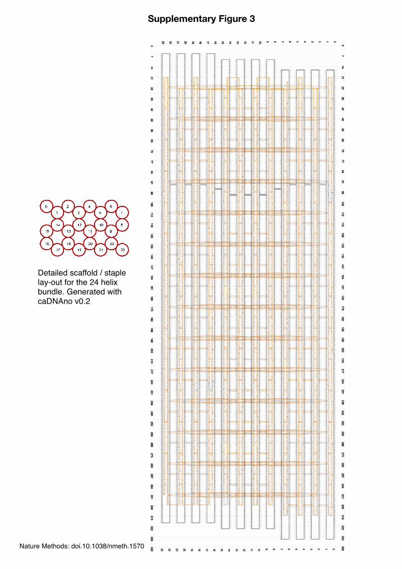
Detailed scaffold / staple lay-out for the 24 helix bundle. Generated with caDNAno v0.2
Supplementary Figure 3
Nature Methods: doi.10.1038/nmeth.1570
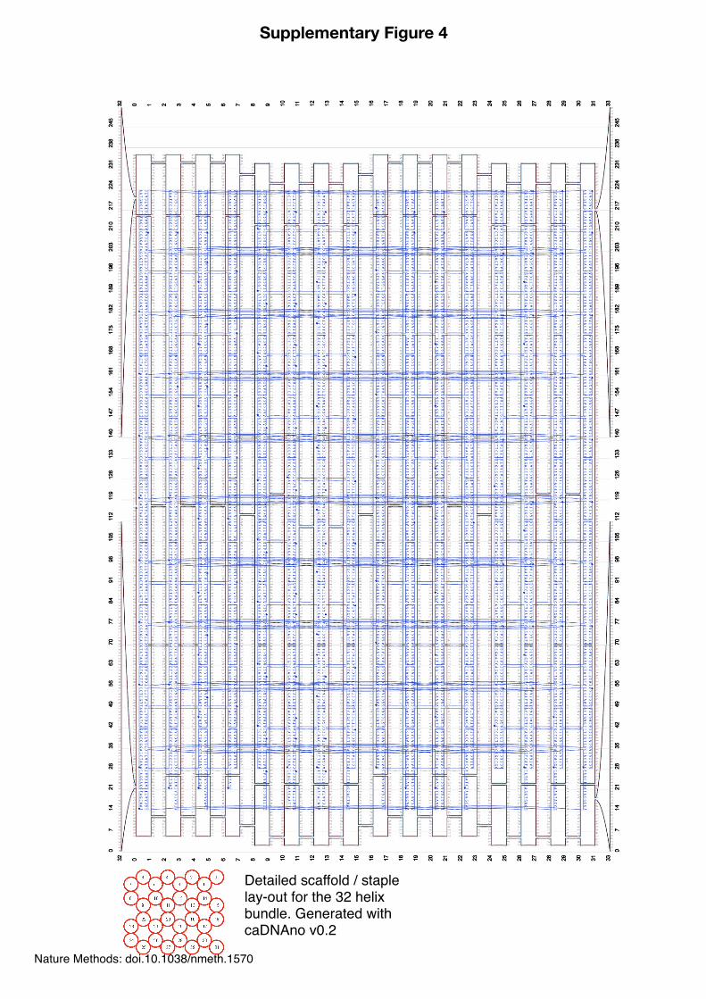
Detailed scaffold / staple lay-out for the 32 helix bundle. Generated with caDNAno v0.2
Supplementary Figure 4
Nature Methods: doi.10.1038/nmeth.1570
obje
ct 1
obje
ct 2
obje
ct 3
obje
ct 4
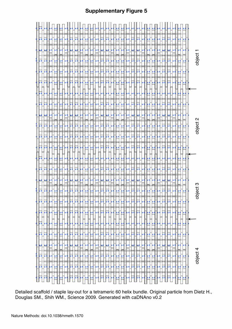
Detailed scaffold / staple lay-out for a tetrameric 60 helix bundle. Original particle from Dietz H., Douglas SM., Shih WM., Science 2009. Generated with caDNAno v0.2
Supplementary Figure 5
Nature Methods: doi.10.1038/nmeth.1570
Supplementary Protocol 1
This protocol is based on Sambrook, J., Russell, D. “Molecular Cloning: A Laboratory Manual”. Third ed.
2001, Cold Spring Harbor Laboratory Press. It was adapted and used for DNA origami purposes with
JM-109 strains first in Douglas, SM., Chou, JJ., Shih, WM. “DNA-nanotube-induced alignment of
membrane proteins for NMR structure determination”, Proc Natl Acad Sci U.S.A., 104, 6644-6648, (2007).
This is a further adaptation for the use with XL-1 Blue strains. Cite Douglas et al when using this protocol.
Step-by-step scaffold production from phage DNA.
(1) Transforming single-stranded M13-derived plasmid DNA into phage-competent E.coli cells.
• Materials:
• Transformation-competent E.Coli strain carrying F' plasmid, or is capable of
growing pili. This protocol works with XL1-Blue. JM-109 is another possible strain.
• LB0 (Luria Bertani) medium.
• Agarplates with tetracyclin [12,5µg/ml], IPTG [40µg/ml], and X-gal [100µg/ml]. If
using JM-109 do NOT include tetracyclin in the plates.
• single stranded phage-plasmid DNA (prepare a dilution with ~ 50 nM concentration)
• single stranded p7249 (i.e wild-type M13mp18 DNA) as a positive control
• Procedure:
• Obtain competent E.coli aliquots (usually 50µl, you'll need at least two if you
include p7249) from -80ºC freezer, let thaw on ice for 20 min.
• Gently pipet 5µl ssDNA on to the cell suspension.
• Let sit on ice for 10 min.
• Heatshock for 30 seconds at 42ºC (60 seconds for p8064)
• Let sit on ice for another 5 min.
• Add 200µl LB0 to the cell suspension
• Shake-incubate at 37ºC for 30 minutes
• Plate onto pre-warmed agarplates. Incubate agarplates overnight at 37ºC
• Store at 4ºC.
Nature Methods: doi.10.1038/nmeth.1570
• Expected Results:
• On the following morning you should discover a bacterial lawn on the plates
covered individual phage plaques that appear like clear "holes" in the lawn. If the
phage density is very high, plaque may also cover larger areas.
• On the wildtype p7249 plate the plaque should be blue, while on clonal variants
such as p7560 or else the plaque should be clear. By the color test you can check
whether inserts are still present and avoid clones that have kicked out the insert
(happens, plaque turn then blue again).
• Comment:
• XL-1 is preferred over XL-10. Plaque do also form with XL-10 but to a much lesser
extent (20-fold reduction).
(2) Growing and harvesting phage in liquid culture.
Note: This protocol is written for XL-1 Blue. If using JM-109, do NOT include tetracyclin selection.
• Materials:
• Agar-plate with M13-derived plaques
• 10 ml LB0 containing tetracyclin in a 125 ml flask
• 250 ml 2xYT Medium containing tetracyclin and 5mM MgCl2 (add 1.25 ml 1M
MgCl2) in a 2-liter flask. Important: Use the 2-liter flask for proper oxygen
circulation.
1. Recipe for 2xYT (use flow hood):
a. Measure ca. 900 ml of distilled water
b. Add 16 g Bacto Tryptone
c. Add 10 g Bacto Yeast Extract
d. Add 5 g NaCl
e. Adjust pH to 7.0 with 5N NaOH
f. Adjust to 1 L distilled water
g. Sterilize by autoclaving
• 10 g dry PEG8000, 7.5 g NaCl
• 10 mM TRIS pH 8.5
Nature Methods: doi.10.1038/nmeth.1570

• Procedure:
• Start overnight culture by scraping -80ºC XL-1 Blue aliquot with a pipet tip followed
by injecting the tip directly into the 10 ml LB0-flask. Shake-incubate at 37ºC
overnight.
• Inoculate the 250 ml 2xYT flask with 3 ml bacterial suspension derived from the
overnight culture.
• Shake-incubate at 37ºC until OD 0.4 is reached. Takes about 1.5 to 2 hrs. It is
important to not overgrow the culture!
• Use the open-end of a pipet tip to scrape plaques from the agar plate prepared
earlier. E.g: gently scrape a lane across an entire plate to collect reasonable
amounts of phages. Inject the scraped-plaques directly into the 250-ml bacteria
culture.
• Shake-incubate at 37ºC at 250 rpm for another 4 hours.
• Pellet bacteria by centrifugation at 4000 rct at 4ºC. Convince yourself that
supernatant is clear.
• Transfer supernatant into a fresh and clear centrifuge bottle. Add 10 g dry PEG8000
and 7.5 g NaCl.
• Mix 30 minutes using magnetic stir bar while incubating bottle in an ice bath. If
there is phage, they should precipitate at this step, causing the solution to turn
cloudy.
• Pellet phage at 4000 rcf for 15 min at 4ºC.
• Decant supernatant, allow bottle to sit at an angle, and carefully remove remainder
of supernatant using a pipette. The remaining pellet/smear should be phage
particles.
• Resuspend pellet/smear in 2.5 ml 10mM Tris pH 8.5 (or 1/100 of original volume).
Active resuspension by up-and-down pipetting may be necessary.
• Pellet residual E.coli cells by centrifugation at 15000 rcf for 15 min at 4ºC.
• Transfer phage supernatant to fresh container. Store at -20ºC or proceed to next
step.
• Expected Results:
Nature Methods: doi.10.1038/nmeth.1570

• Step 8 should result in a cloudy solution and a visible pellet/smear should appear
when pelleting the phage. If this does not happen, the yield will be probably very
low. Consider re-starting from the beginning.
(3) Purify ssDNA from phage / stripping proteins by alkaline/detergent denaturation.
• Materials:
• Lysis-Buffer (0.2 M NaOH, 1% SDS or the one from Qiagen Plasmid Prep Kit)
• Neutralization-Buffer (3 M KOAc pH 5.5 or the one from Qiagen Plasmid Prep Kit)
• Pure Ethanol and 75% Ethanol.
• 10 mM TRIS-base buffer pH 8.5
• Procedure:
• Add 2 volumes (5 ml if continuing from step (2)) lysis buffer, gently mix by inversions.
• Add 1.5 volumes (3.75 ml if continuing from step (2)) neutralization buffer, gently mix by
inversions.
• Incubate in ice-water bath for 15 minutes.
• Spin at 16000 rcf at 4ºC for 10 minutes.
• Transfer supernatant into fresh container (recommend 50 ml falcon tube).
• Add 1 volume pure ethanol (ca. 8 ml) to the transferred supernatant.
• Incubate in ice-water bath for 30 minutes.
• Spin at 16000 rcf for 15 minutes at 4ºC.
• Discard supernatant. Carefully pipet-out residual supernatant.
• Add 1.5 ml 75% ethanol to the pellet. Mix by swirling.
• Incubate in ice-water bath for 10 minutes.
• Spin at 16000 rcf for 15 minutes at 4ºC.
• Discard supernatant. Carefully pipet-out residual supernatant.
• Resuspend pellet in 1 ml 10 mM TRIS pH 8.5.
• Use spectrophotometer to estimate concentration of resuspended ssDNA.
• Run a 2% agarose gel containing 11 mM MgCl2 and 0.5 mg/ml EtBr. Running buffer 0.5x
TBE with 11mM MgCls. Include a positive control!
Nature Methods: doi.10.1038/nmeth.1570
• Store purified DNA at -20ºC.
• Expected Results: expect a yield of approx 1 mg ssDNA for this prep-scale at a concentration of
about 350 nM.
Nature Methods: doi.10.1038/nmeth.1570
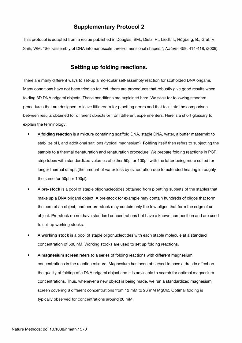
Supplementary Protocol 2
This protocol is adapted from a recipe published in Douglas, SM., Dietz, H., Liedl, T., Högberg, B., Graf, F.,
Shih, WM. “Self-assembly of DNA into nanoscale three-dimensional shapes.”, Nature, 459, 414-418, (2009).
Setting up folding reactions.
There are many different ways to set-up a molecular self-assembly reaction for scaffolded DNA origami.
Many conditions have not been tried so far. Yet, there are procedures that robustly give good results when
folding 3D DNA origami objects. These conditions are explained here. We seek for following standard
procedures that are designed to leave little room for pipetting errors and that facilitate the comparison
between results obtained for different objects or from different experimenters. Here is a short glossary to
explain the terminology:
• A folding reaction is a mixture containing scaffold DNA, staple DNA, water, a buffer mastermix to
stabilize pH, and additional salt ions (typical magnesium). Folding itself then refers to subjecting the
sample to a thermal denaturation and renaturation procedure. We prepare folding reactions in PCR
strip tubes with standardized volumes of either 50µl or 100µl, with the latter being more suited for
longer thermal ramps (the amount of water loss by evaporation due to extended heating is roughly
the same for 50µl or 100µl).
• A pre-stock is a pool of staple oligonucleotides obtained from pipetting subsets of the staples that
make up a DNA origami object. A pre-stock for example may contain hundreds of oligos that form
the core of an object, another pre-stock may contain only the few oligos that form the edge of an
object. Pre-stock do not have standard concentrations but have a known composition and are used
to set-up working stocks.
• A working stock is a pool of staple oligonucleotides with each staple molecule at a standard
concentration of 500 nM. Working stocks are used to set up folding reactions.
• A magnesium screen refers to a series of folding reactions with different magnesium
concentrations in the reaction mixture. Magnesium has been observed to have a drastic effect on
the quality of folding of a DNA origami object and it is advisable to search for optimal magnesium
concentrations. Thus, whenever a new object is being made, we run a standardized magnesium
screen covering 8 different concentrations from 12 mM to 26 mM MgCl2. Optimal folding is
typically observed for concentrations around 20 mM.
Nature Methods: doi.10.1038/nmeth.1570

Step 1: Write down a pipetting guide
A useful starting point is to develop a pipetting guide for the DNA origami shape as exemplified by the
scheme shown below that was prepared for a set of staple oligonucleotides on two 96-well plates named
HD_P013 and HD_P014 at normalized concentration of 100 µM each. The guide is useful for preparing the
pre- and working stocks. It is advisable to prepare the pipetting guide together with the staple order and to
store it for later reference.
Step 3: Pipet the pre- and working stocks according to the pipetting guide
For this step one will need a multi-channel pipette and some patience. Pool for example 10µl from source
wells belonging to a certain structural module of the target structure into a common reservoir. This will
become a prestock. To prepare the working stock, combine stoichiometric volumes from each prestock
(see the column indicated with Σ in the scheme above) into a new tube. Add water to normalize to a desired
target concentration.
Nature Methods: doi.10.1038/nmeth.1570
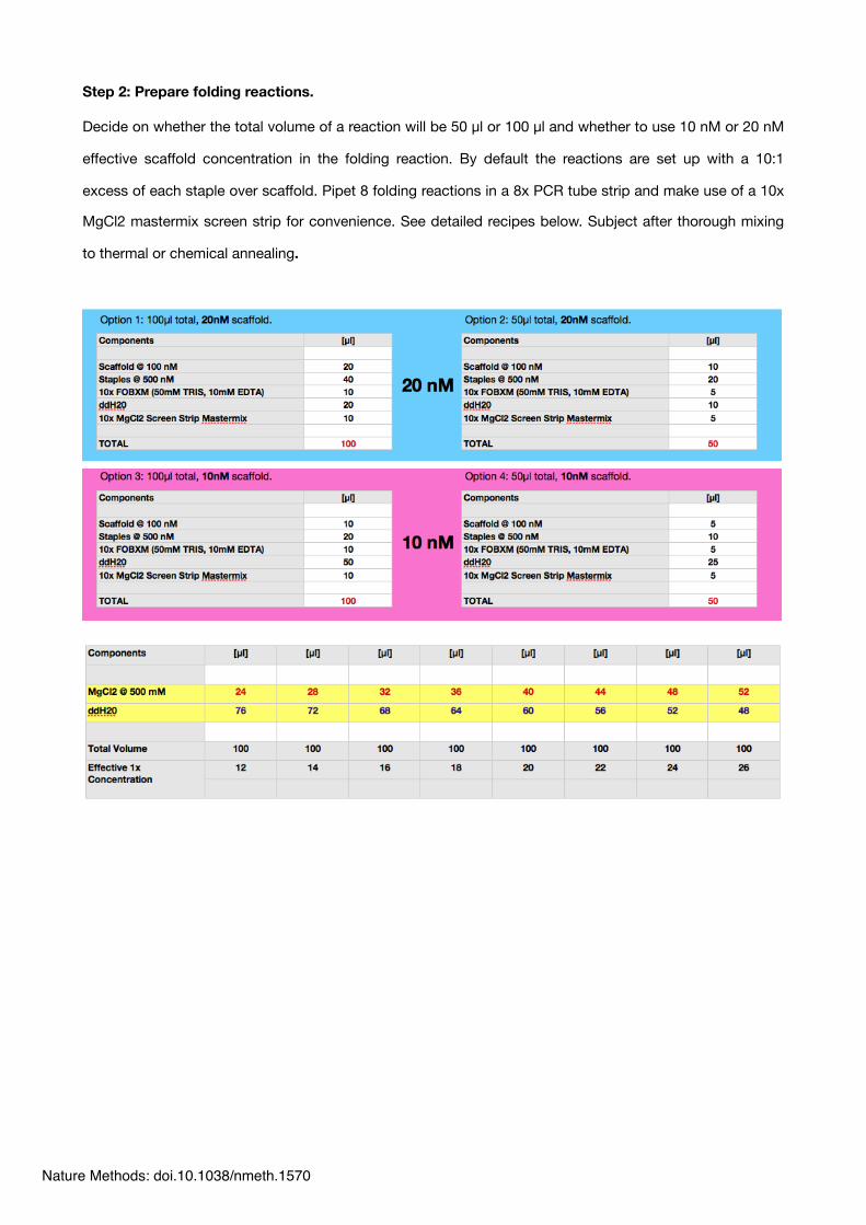
Step 2: Prepare folding reactions.
Decide on whether the total volume of a reaction will be 50 µl or 100 µl and whether to use 10 nM or 20 nM
effective scaffold concentration in the folding reaction. By default the reactions are set up with a 10:1
excess of each staple over scaffold. Pipet 8 folding reactions in a 8x PCR tube strip and make use of a 10x
MgCl2 mastermix screen strip for convenience. See detailed recipes below. Subject after thorough mixing
to thermal or chemical annealing.
Nature Methods: doi.10.1038/nmeth.1570
Supplementary Protocol 3
This protocol is adapted from Douglas, SM., Dietz, H., Liedl, T., Högberg, B., Graf, F., Shih, WM. “Self-
assembly of DNA into nanoscale three-dimensional shapes.”, Nature, 459, 414-418, (2009).
Agarose Gel Electrophoresis (EtBr) with DNA origami objects
Gel Preparation
Prepare a 2% agarose gel. (Here we assume 125 ml gel slab volume)
• weigh 2.5 g agarose ultra pure (Invitrogen) into a beaker
• fill up to 125 g with 0.5x TBE-Puffer
• boil in microwave until the agarose is completely dissolved (2 min @ 800 watts)
• fill up again to 125 g with ddH2O
• cool it under the water tap until hand warm
• add 1 ml of 1.375 M MgCl2 solution (gives total MgCl2-concentration of 11mM)
• add 7 µl ethidium bromide from a 10 mg/ml stock solution)
• fill the gel tray and install desired comb immediatly
• once gel is solid, fill the gel box with TBE/11mM MgCl2 buffer
• remove comb
Gel Loading
(applies for folding-reactions containing ~10nM scaffold DNA)
sample preparation
• mix gently 12 µl sample with 3 µl 6x-loading dye (containing at least 30% glycerole)
• pipet the mix into a gel pocket
reference preparation
• mix
• 1.2 µl single-stranded phage DNA (@100nM)
• 10.8 µl ddH2O
• 3 µl 6x-loading dye
• load the mix into a gel pocket
Nature Methods: doi.10.1038/nmeth.1570
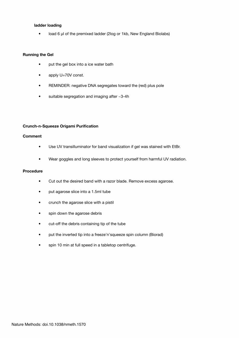
ladder loading
• load 6 µl of the premixed ladder (2log or 1kb, New England Biolabs)
Running the Gel
• put the gel box into a ice water bath
• apply U=70V const.
• REMINDER: negative DNA segregates toward the (red) plus pole
• suitable segregation and imaging after ~3-4h
Crunch-n-Squeeze Origami Purification
Comment
• Use UV transilluminator for band visualization if gel was stained with EtBr.
• Wear goggles and long sleeves to protect yourself from harmful UV radiation.
Procedure
• Cut out the desired band with a razor blade. Remove excess agarose.
• put agarose slice into a 1.5ml tube
• crunch the agarose slice with a pistil
• spin down the agarose debris
• cut-off the debris containing tip of the tube
• put the inverted tip into a freeze'n'squeeze spin column (Biorad)
• spin 10 min at full speed in a tabletop centrifuge.
Nature Methods: doi.10.1038/nmeth.1570
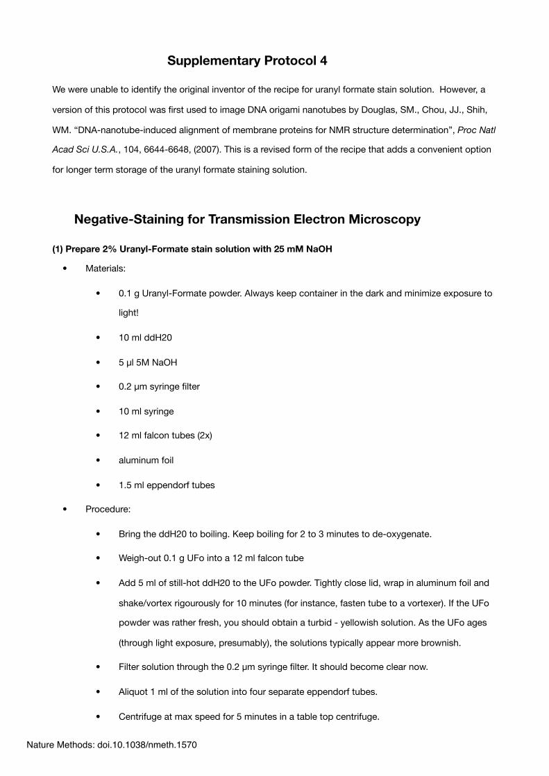
Supplementary Protocol 4
We were unable to identify the original inventor of the recipe for uranyl formate stain solution. However, a
version of this protocol was first used to image DNA origami nanotubes by Douglas, SM., Chou, JJ., Shih,
WM. “DNA-nanotube-induced alignment of membrane proteins for NMR structure determination”, Proc Natl
Acad Sci U.S.A., 104, 6644-6648, (2007). This is a revised form of the recipe that adds a convenient option
for longer term storage of the uranyl formate staining solution.
Negative-Staining for Transmission Electron Microscopy
(1) Prepare 2% Uranyl-Formate stain solution with 25 mM NaOH
• Materials:
• 0.1 g Uranyl-Formate powder. Always keep container in the dark and minimize exposure to
light!
• 10 ml ddH20
• 5 µl 5M NaOH
• 0.2 µm syringe filter
• 10 ml syringe
• 12 ml falcon tubes (2x)
• aluminum foil
• 1.5 ml eppendorf tubes
• Procedure:
• Bring the ddH20 to boiling. Keep boiling for 2 to 3 minutes to de-oxygenate.
• Weigh-out 0.1 g UFo into a 12 ml falcon tube
• Add 5 ml of still-hot ddH20 to the UFo powder. Tightly close lid, wrap in aluminum foil and
shake/vortex rigourously for 10 minutes (for instance, fasten tube to a vortexer). If the UFo
powder was rather fresh, you should obtain a turbid - yellowish solution. As the UFo ages
(through light exposure, presumably), the solutions typically appear more brownish.
• Filter solution through the 0.2 µm syringe filter. It should become clear now.
• Aliquot 1 ml of the solution into four separate eppendorf tubes.
• Centrifuge at max speed for 5 minutes in a table top centrifuge.
Nature Methods: doi.10.1038/nmeth.1570
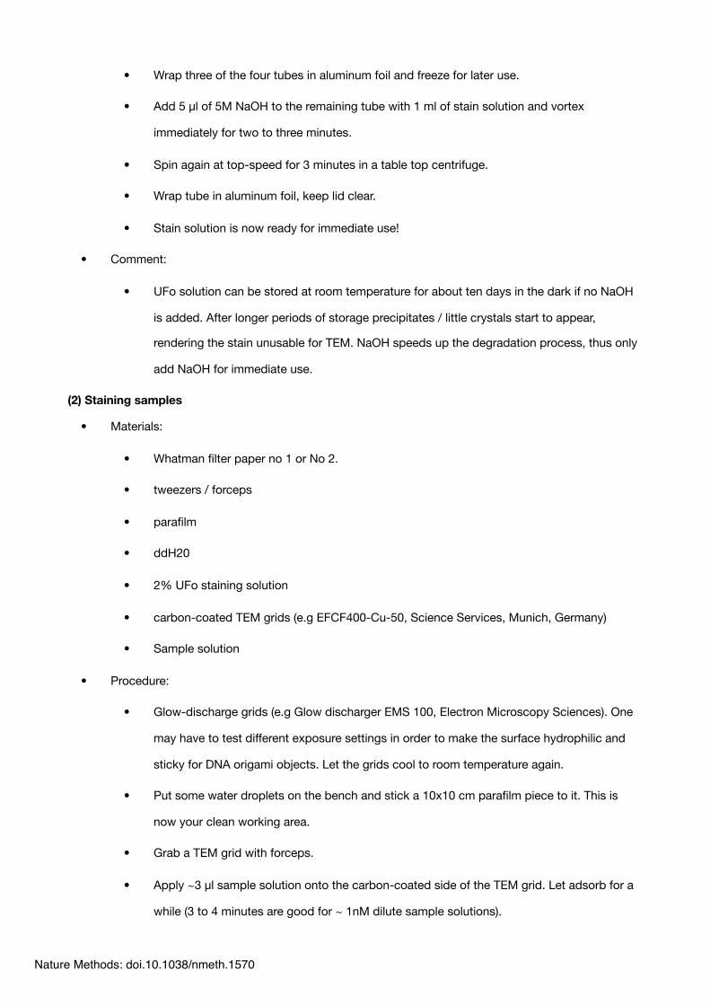
• Wrap three of the four tubes in aluminum foil and freeze for later use.
• Add 5 µl of 5M NaOH to the remaining tube with 1 ml of stain solution and vortex
immediately for two to three minutes.
• Spin again at top-speed for 3 minutes in a table top centrifuge.
• Wrap tube in aluminum foil, keep lid clear.
• Stain solution is now ready for immediate use!
• Comment:
• UFo solution can be stored at room temperature for about ten days in the dark if no NaOH
is added. After longer periods of storage precipitates / little crystals start to appear,
rendering the stain unusable for TEM. NaOH speeds up the degradation process, thus only
add NaOH for immediate use.
(2) Staining samples
• Materials:
• Whatman filter paper no 1 or No 2.
• tweezers / forceps
• parafilm
• ddH20
• 2% UFo staining solution
• carbon-coated TEM grids (e.g EFCF400-Cu-50, Science Services, Munich, Germany)
• Sample solution
• Procedure:
• Glow-discharge grids (e.g Glow discharger EMS 100, Electron Microscopy Sciences). One
may have to test different exposure settings in order to make the surface hydrophilic and
sticky for DNA origami objects. Let the grids cool to room temperature again.
• Put some water droplets on the bench and stick a 10x10 cm parafilm piece to it. This is
now your clean working area.
• Grab a TEM grid with forceps.
• Apply ~3 µl sample solution onto the carbon-coated side of the TEM grid. Let adsorb for a
while (3 to 4 minutes are good for ~ 1nM dilute sample solutions).
Nature Methods: doi.10.1038/nmeth.1570

• Meanwhile, apply a 25 µl stain solution droplet onto the para film.
• Use filter paper edge to drain excess liquid from the edge of the grid. Do not touch the grid
surface. Remaining liquid film will evaporate in a few seconds, so act quickly now.
• Immerse grid sample-side first into the stain-solution droplet. Incubate for 40 seconds.
• Use filter paper edge to dap off excess liquid from the edge of the grid. Do not touch the
grid surface.
• Let the grid dry completely before injecting into the TEM! (30 minutes)
• Ready for imaging!
• Comments:
• Depending on the carbon quality, sample concentration / composition, incubation times
may have to be varied. Washing the grid with 0.5 MgCl2 prior to applying the sample can
influence orientations on the grid (more interface views).
Preparing Custom Grids for Transmission Electron Microscopy
(1) Coat grids with a thin collodion plastic film.
• Materials:
• Collodion
• minimum 20 cm diameter bowl/basin
• ddH20
• TEM copper grids 200 or 400
• vellum paper ('Pergament-Papier')
• tweezers, forceps
• razor blade
• 200 pipet
• Procedure:
• Completetly fill basin with ddH20 right to the rim
• Use razor blade to shorten a 200er pipet tip to create a 3mm diameter aperture
• Pipet out 50µl collodion solution.
Nature Methods: doi.10.1038/nmeth.1570

• Eject the collodion from approx 10 cm onto the calm water surface. CAUTION: collodion is
toxic! Ensure proper ventilation and hold breath while handling the collodion!
• A collodion film will spread across the water surface and harden. Wait for 5 min.
• Use forceps to position copper grids onto the collodion film. Put shiny (specular-reflecting)
side of the grids facing the collodion. Arrange in a neat hexagonal or square pattern.
• Position vellum paper on top of grids. Let soak with water.
• Cut collodion film around the circumference of the vellum paper by using the razor blade.
• Carefully pick up the vellum paper at one corner/edge and pull out of the water.
• Turn the vellum paper with the grids facing up, put into petri dish, partially cover and let dry
overnight in a clean, dust free area (i.e. in a hood)
• Ready!
(2) Evaporate carbon film onto grids.
Nature Methods: doi.10.1038/nmeth.1570
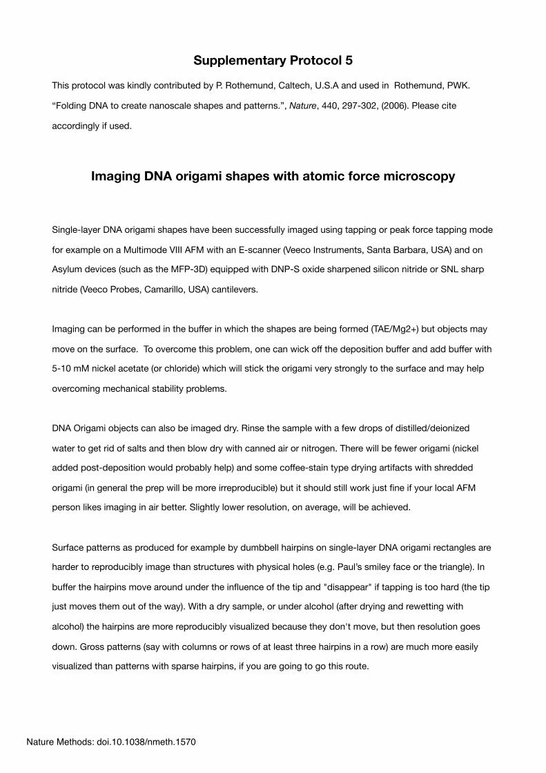
Supplementary Protocol 5
This protocol was kindly contributed by P. Rothemund, Caltech, U.S.A and used in Rothemund, PWK.
“Folding DNA to create nanoscale shapes and patterns.”, Nature, 440, 297-302, (2006). Please cite
accordingly if used.
Imaging DNA origami shapes with atomic force microscopy
Single-layer DNA origami shapes have been successfully imaged using tapping or peak force tapping mode
for example on a Multimode VIII AFM with an E-scanner (Veeco Instruments, Santa Barbara, USA) and on
Asylum devices (such as the MFP-3D) equipped with DNP-S oxide sharpened silicon nitride or SNL sharp
nitride (Veeco Probes, Camarillo, USA) cantilevers.
Imaging can be performed in the buffer in which the shapes are being formed (TAE/Mg2+) but objects may
move on the surface. To overcome this problem, one can wick off the deposition buffer and add buffer with
5-10 mM nickel acetate (or chloride) which will stick the origami very strongly to the surface and may help
overcoming mechanical stability problems.
DNA Origami objects can also be imaged dry. Rinse the sample with a few drops of distilled/deionized
water to get rid of salts and then blow dry with canned air or nitrogen. There will be fewer origami (nickel
added post-deposition would probably help) and some coffee-stain type drying artifacts with shredded
origami (in general the prep will be more irreproducible) but it should still work just fine if your local AFM
person likes imaging in air better. Slightly lower resolution, on average, will be achieved.
Surface patterns as produced for example by dumbbell hairpins on single-layer DNA origami rectangles are
harder to reproducibly image than structures with physical holes (e.g. Paul’s smiley face or the triangle). In
buffer the hairpins move around under the influence of the tip and "disappear" if tapping is too hard (the tip
just moves them out of the way). With a dry sample, or under alcohol (after drying and rewetting with
alcohol) the hairpins are more reproducibly visualized because they don't move, but then resolution goes
down. Gross patterns (say with columns or rows of at least three hairpins in a row) are much more easily
visualized than patterns with sparse hairpins, if you are going to go this route.
Nature Methods: doi.10.1038/nmeth.1570
Supplementary Note 1
Refer to Douglas, SM., Marblestone, AH., Teerapittayanon, S., Vazquez, A., Church, GM., Shih, WM. “Rapid
prototyping of 3D DNA-origami shapes with caDNAno”, Nucleic Acids Res, 37, 5001-5006, (2009) and
please visit http://cadnano.org for online tutorials to the design of DNA origami shapes with caDNAno. We
provide here a short introduction that may help understanding the concept of caDNAno-generated
scaffold / staple lay-outs and source files.
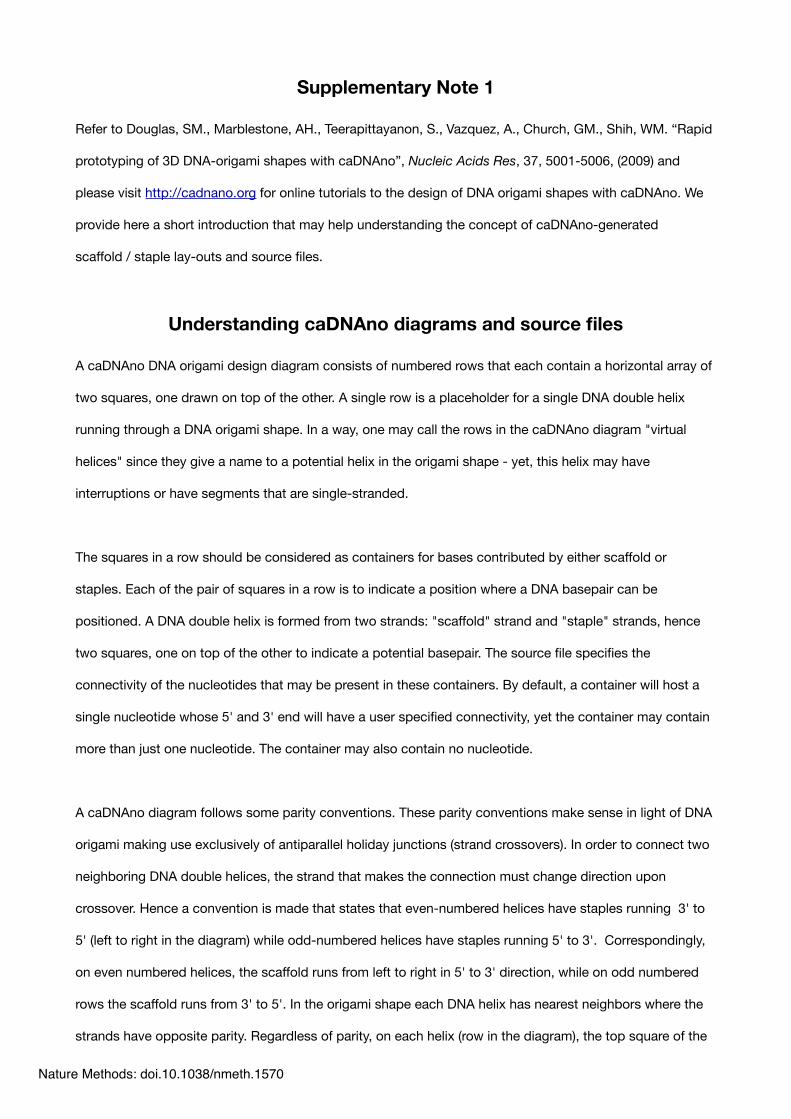
Understanding caDNAno diagrams and source files
A caDNAno DNA origami design diagram consists of numbered rows that each contain a horizontal array of
two squares, one drawn on top of the other. A single row is a placeholder for a single DNA double helix
running through a DNA origami shape. In a way, one may call the rows in the caDNAno diagram "virtual
helices" since they give a name to a potential helix in the origami shape - yet, this helix may have
interruptions or have segments that are single-stranded.
The squares in a row should be considered as containers for bases contributed by either scaffold or
staples. Each of the pair of squares in a row is to indicate a position where a DNA basepair can be
positioned. A DNA double helix is formed from two strands: "scaffold" strand and "staple" strands, hence
two squares, one on top of the other to indicate a potential basepair. The source file specifies the
connectivity of the nucleotides that may be present in these containers. By default, a container will host a
single nucleotide whose 5' and 3' end will have a user specified connectivity, yet the container may contain
more than just one nucleotide. The container may also contain no nucleotide.
A caDNAno diagram follows some parity conventions. These parity conventions make sense in light of DNA
origami making use exclusively of antiparallel holiday junctions (strand crossovers). In order to connect two
neighboring DNA double helices, the strand that makes the connection must change direction upon
crossover. Hence a convention is made that states that even-numbered helices have staples running 3' to
5' (left to right in the diagram) while odd-numbered helices have staples running 5' to 3'. Correspondingly,
on even numbered helices, the scaffold runs from left to right in 5' to 3' direction, while on odd numbered
rows the scaffold runs from 3' to 5'. In the origami shape each DNA helix has nearest neighbors where the
strands have opposite parity. Regardless of parity, on each helix (row in the diagram), the top square of the
Nature Methods: doi.10.1038/nmeth.1570
duplex-square-array always refers to a strand running from 5' to 3', while the bottom square refers to a
strand running 3' to 5'. Thus, the scaffold portion of a DNA double helix is drawn in the top squares on even
rows (helices), while it is drawn in the bottom squares on odd rows. The scaffold portion in a row is always
labeled in cyan-blue, while the staple color may be chosen by the user.
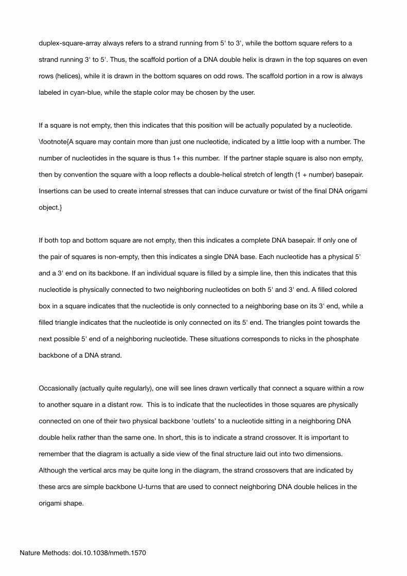
If a square is not empty, then this indicates that this position will be actually populated by a nucleotide.
\footnote{A square may contain more than just one nucleotide, indicated by a little loop with a number. The
number of nucleotides in the square is thus 1+ this number. If the partner staple square is also non empty,
then by convention the square with a loop reflects a double-helical stretch of length (1 + number) basepair.
Insertions can be used to create internal stresses that can induce curvature or twist of the final DNA origami
object.}
If both top and bottom square are not empty, then this indicates a complete DNA basepair. If only one of
the pair of squares is non-empty, then this indicates a single DNA base. Each nucleotide has a physical 5'
and a 3' end on its backbone. If an individual square is filled by a simple line, then this indicates that this
nucleotide is physically connected to two neighboring nucleotides on both 5' and 3' end. A filled colored
box in a square indicates that the nucleotide is only connected to a neighboring base on its 3' end, while a
filled triangle indicates that the nucleotide is only connected on its 5' end. The triangles point towards the
next possible 5' end of a neighboring nucleotide. These situations corresponds to nicks in the phosphate
backbone of a DNA strand.
Occasionally (actually quite regularly), one will see lines drawn vertically that connect a square within a row
to another square in a distant row. This is to indicate that the nucleotides in those squares are physically
connected on one of their two physical backbone ‘outlets’ to a nucleotide sitting in a neighboring DNA
double helix rather than the same one. In short, this is to indicate a strand crossover. It is important to
remember that the diagram is actually a side view of the final structure laid out into two dimensions.
Although the vertical arcs may be quite long in the diagram, the strand crossovers that are indicated by
these arcs are simple backbone U-turns that are used to connect neighboring DNA double helices in the
origami shape.
Nature Methods: doi.10.1038/nmeth.1570
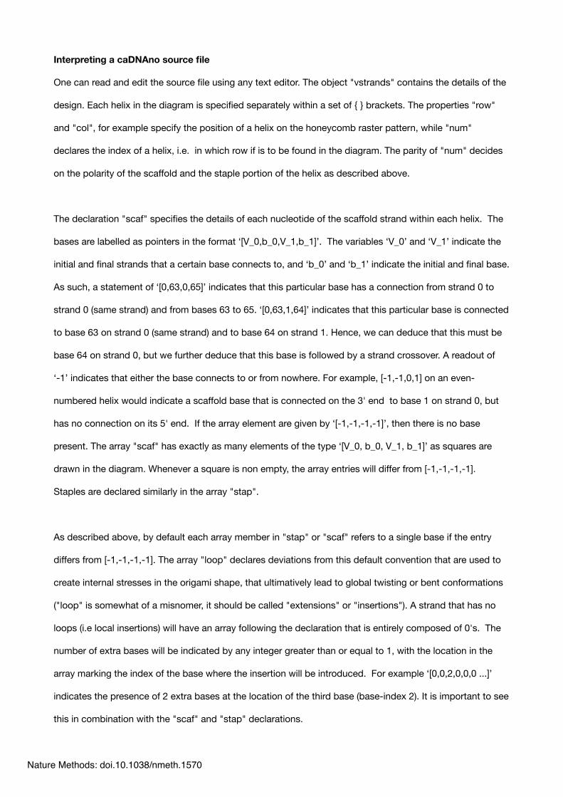
Interpreting a caDNAno source file
One can read and edit the source file using any text editor. The object "vstrands" contains the details of the
design. Each helix in the diagram is specified separately within a set of { } brackets. The properties "row"
and "col", for example specify the position of a helix on the honeycomb raster pattern, while "num"
declares the index of a helix, i.e. in which row if is to be found in the diagram. The parity of "num" decides
on the polarity of the scaffold and the staple portion of the helix as described above.
The declaration "scaf" specifies the details of each nucleotide of the scaffold strand within each helix. The
bases are labelled as pointers in the format ‘[V_0,b_0,V_1,b_1]’. The variables ‘V_0’ and ‘V_1’ indicate the
initial and final strands that a certain base connects to, and ‘b_0’ and ‘b_1’ indicate the initial and final base.
As such, a statement of ‘[0,63,0,65]’ indicates that this particular base has a connection from strand 0 to
strand 0 (same strand) and from bases 63 to 65. ‘[0,63,1,64]’ indicates that this particular base is connected
to base 63 on strand 0 (same strand) and to base 64 on strand 1. Hence, we can deduce that this must be
base 64 on strand 0, but we further deduce that this base is followed by a strand crossover. A readout of
‘-1’ indicates that either the base connects to or from nowhere. For example, [-1,-1,0,1] on an even-
numbered helix would indicate a scaffold base that is connected on the 3' end to base 1 on strand 0, but
has no connection on its 5' end. If the array element are given by ‘[-1,-1,-1,-1]’, then there is no base
present. The array "scaf" has exactly as many elements of the type ‘[V_0, b_0, V_1, b_1]’ as squares are
drawn in the diagram. Whenever a square is non empty, the array entries will differ from [-1,-1,-1,-1].
Staples are declared similarly in the array "stap".
As described above, by default each array member in "stap" or "scaf" refers to a single base if the entry
differs from [-1,-1,-1,-1]. The array "loop" declares deviations from this default convention that are used to
create internal stresses in the origami shape, that ultimatively lead to global twisting or bent conformations
("loop" is somewhat of a misnomer, it should be called "extensions" or "insertions"). A strand that has no
loops (i.e local insertions) will have an array following the declaration that is entirely composed of 0's. The
number of extra bases will be indicated by any integer greater than or equal to 1, with the location in the
array marking the index of the base where the insertion will be introduced. For example ‘[0,0,2,0,0,0 ...]’
indicates the presence of 2 extra bases at the location of the third base (base-index 2). It is important to see
this in combination with the "scaf" and "stap" declarations.
Nature Methods: doi.10.1038/nmeth.1570
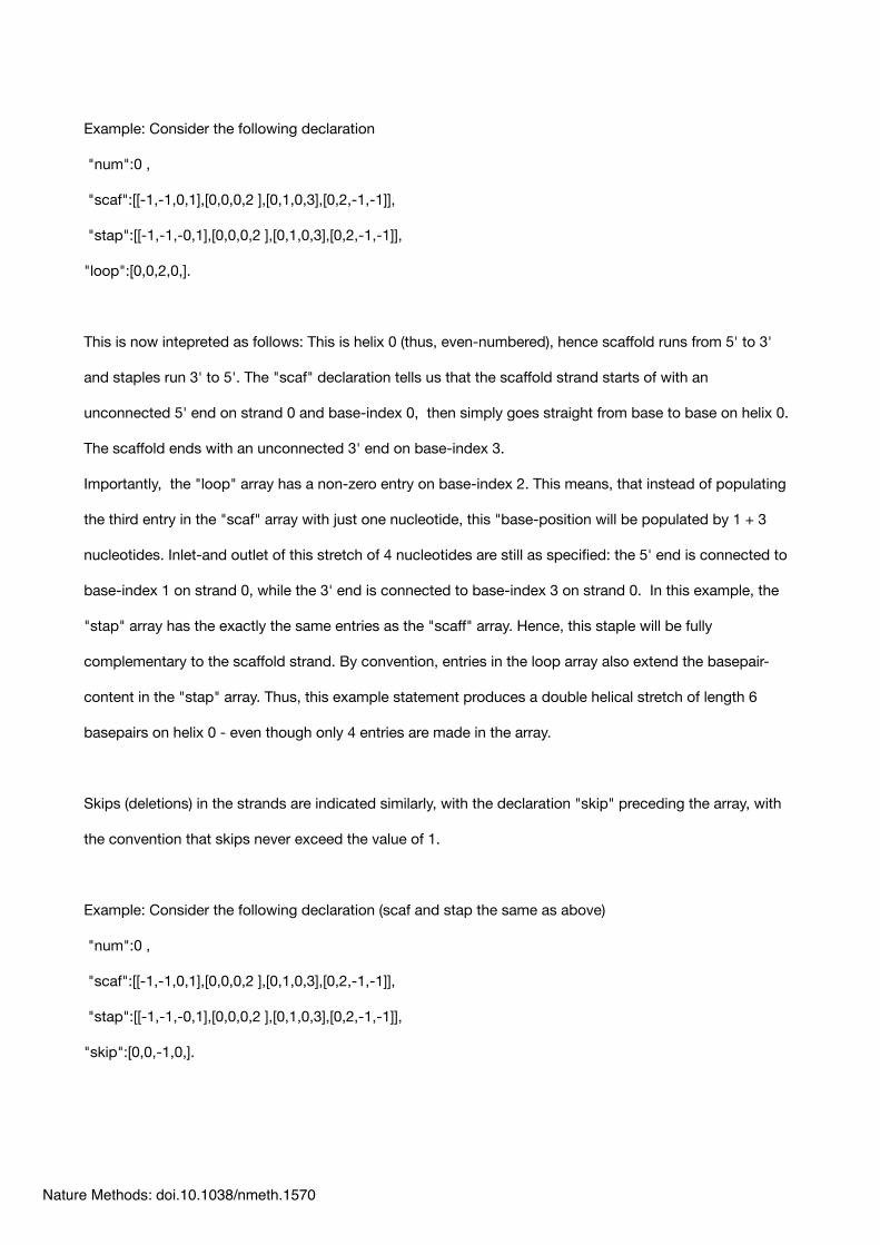
Example: Consider the following declaration
"num":0 ,
"scaf":[[-1,-1,0,1],[0,0,0,2 ],[0,1,0,3],[0,2,-1,-1]],
"stap":[[-1,-1,-0,1],[0,0,0,2 ],[0,1,0,3],[0,2,-1,-1]],
"loop":[0,0,2,0,].
This is now intepreted as follows: This is helix 0 (thus, even-numbered), hence scaffold runs from 5' to 3'
and staples run 3' to 5'. The "scaf" declaration tells us that the scaffold strand starts of with an
unconnected 5' end on strand 0 and base-index 0, then simply goes straight from base to base on helix 0.
The scaffold ends with an unconnected 3' end on base-index 3.
Importantly, the "loop" array has a non-zero entry on base-index 2. This means, that instead of populating
the third entry in the "scaf" array with just one nucleotide, this "base-position will be populated by 1 + 3
nucleotides. Inlet-and outlet of this stretch of 4 nucleotides are still as specified: the 5' end is connected to
base-index 1 on strand 0, while the 3' end is connected to base-index 3 on strand 0. In this example, the
"stap" array has the exactly the same entries as the "scaff" array. Hence, this staple will be fully
complementary to the scaffold strand. By convention, entries in the loop array also extend the basepair-
content in the "stap" array. Thus, this example statement produces a double helical stretch of length 6
basepairs on helix 0 - even though only 4 entries are made in the array.
Skips (deletions) in the strands are indicated similarly, with the declaration "skip" preceding the array, with
the convention that skips never exceed the value of 1.
Example: Consider the following declaration (scaf and stap the same as above)
"num":0 ,
"scaf":[[-1,-1,0,1],[0,0,0,2 ],[0,1,0,3],[0,2,-1,-1]],
"stap":[[-1,-1,-0,1],[0,0,0,2 ],[0,1,0,3],[0,2,-1,-1]],
"skip":[0,0,-1,0,].
Nature Methods: doi.10.1038/nmeth.1570
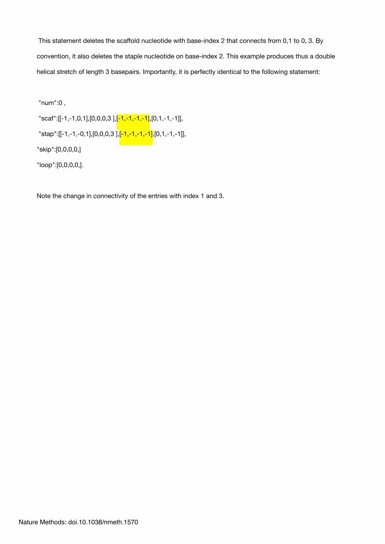
This statement deletes the scaffold nucleotide with base-index 2 that connects from 0,1 to 0, 3. By
convention, it also deletes the staple nucleotide on base-index 2. This example produces thus a double
helical stretch of length 3 basepairs. Importantly, it is perfectly identical to the following statement:
"num":0 ,
"scaf":[[-1,-1,0,1],[0,0,0,3 ],[-1,-1,-1,-1],[0,1,-1,-1]],
"stap":[[-1,-1,-0,1],[0,0,0,3 ],[-1,-1,-1,-1],[0,1,-1,-1]],
"skip":[0,0,0,0,]
"loop":[0,0,0,0,].
Note the change in connectivity of the entries with index 1 and 3.
Nature Methods: doi.10.1038/nmeth.1570
Supplementary Note 2
Please refer to http://cando.dna-origami.org for submitting files for analysis and additional resources.
Computer-aided engineering for DNA origami: ‘CanDo’.
1. DNA model
DNA double helices are modeled as continuous and homogeneous, isotropic Euler–Bernouilli beams
characterized by stretch, twist, and bend moduli (1). This approximation ignores potential sequence-specific
mechanical properties. The DNA double-helix is assumed to have axial rise 0.34 nm/bp and diameter 2.25
nm (2) with stretch modulus 1100 pN, bend modulus 230 pNnm2, and twist modulus 460 pNnm2 (3-7).
Twist-stretch coupling is ignored in the current implementation (3). Strand crossovers that couple
deformations of neighboring helices are modeled as rigid links that fully constrain the stretch, twist, and
bend degrees of freedom of joined helices. Two-node Hermitian beam finite elements are used in the finite
element method, which describes stretch, bend, and twist deformations using three translational degrees of
freedom, two rotational degrees of freedom for bending, and one rotational degree of freedom for twisting
at each finite element node along the neutral axis of the beam.
2. Prediction of 3D structure
caDNAno design files are parsed by CanDo to read geometric data including helix location on the cubic or
honeycomb lattice, locations of inserted and/or deleted basepairs, and crossover positions. An initial
configuration is first generated where all helices are arranged linearly and co-axially in space. Next, finite
element nodes of basepairs that are coupled by inter-helical crossovers are displaced axially to the
corresponding crossover positions based on the crossover spacing rule from the average helicity of B-form
DNA. In this deformed configuration, rigid links are placed between nodes joined by a crossover, after which
all external loads are released so that the structure is allowed to deform to satisfy the full equations of
equilibrium (8). The deformation analysis may be performed using either geometrically linear or nonlinear
analysis (8).
Nature Methods: doi.10.1038/nmeth.1570
3. Calculation of 3D structural flexibility
Root-mean-square fluctuations (RMSF) of the deformed 3D structure in thermal equilibrium are calculated in
the standard way (9,10) using the equipartition theorem of statistical mechanics and normal mode analysis
(NMA). The RMSF for each FE node i is calculated by considering contributions from 200 low frequency
normal modes using where is the displacement vector of node i
due to normal mode k, is the eigenvalue associated with mode k, is the Boltzmann constant and
is temperature, assumed to be 298 K.
Detailed description about the model and the analysis procedure will appear in a manuscript in preparation
by Kim, D.-N., Dietz H., and Bathe, M.
1.! Peters, J.P. and Maher, L.J. (2010) DNA curvature and flexibility in vitro and in vivo. Q Rev Biophys,
43, 23-63.
2.! Dietz, H., Douglas, S.M. and Shih, W.M. (2009) Folding DNA into twisted and curved nanoscale
shapes. Science, 325, 725-730.
3.! Gore, J., Bryant, Z., Nollmann, M., Le, M.U., Cozzarelli, N.R. and Bustamante, C. (2006) DNA
overwinds when stretched. Nature, 442, 836-839.
4.! Bustamante, C., Smith, S.B., Liphardt, J. and Smith, D. (2000) Single-molecule studies of DNA
mechanics. Curr. Opin. Struct. Biol., 10, 279-285.
5.! Bryant, Z., Stone, M.D., Gore, J., Smith, S.B., Cozzarelli, N.R. and Bustamante, C. (2003) Structural
transitions and elasticity from torque measurements on DNA. Nature, 424, 338-341.
6.! Smith, S.B., Cui, Y.J. and Bustamante, C. (1996) Overstretching B-DNA: The elastic response of
individual double-stranded and single-stranded DNA molecules. Science, 271, 795-799.
7.! Wang, M.D., Yin, H., Landick, R., Gelles, J. and Block, S.M. (1997) Stretching DNA with optical
tweezers. Biophys J, 72, 1335-1346.
8.! Bathe, K.J. (1996) Finite Element Procedures. Prentice Hall Inc., Upper Saddle River, New Jersey.
9.! Brooks, B.R., Janezic, D. and Karplus, M. (1995) Harmonic analysis of large systems. 1.
Methodology. J. Comput. Chem., 16, 1522-1542.
Nature Methods: doi.10.1038/nmeth.1570

10.! Kim, D.-N., Nguyen, C.-T. and Bathe, M. (In press) Conformational dynamics of supramolecular
protein assemblies. J Struct Biol.
Nature Methods: doi.10.1038/nmeth.1570
Supplementary Methods
Thermal stability of DNA origami structures
Melting profiles for the three test structures as well as a 6 helix bundle and a 20 nucleotide DNA duplex
were taken using a real time PCR machine (Stratagene MX3005P, Agilent Inc). DNA origami objects were
purified by agarose gel electrophoresis and subsequent crunch and squeeze purification resulting in a yield
of approximately 4 nM (~20% yield). These structures were diluted to a final concentration of ~1 nM in a
total volume of 50 µl in a solution containing 16 mM MgCl2, 5 mM TRIS, 1 mM EDTA, and 5 mM NaCl, as
well as 1 µM of a specific intercalating dye SYBR green (Invitrogen) whose fluorescence is ~1000 times
enhanced when bound to double-stranded DNA. The buffer conditions were chosen to be similar to the
optimal folding conditions for all structures. The mixture was heated from 25 to 80 oC at a speed of 0.29
oC/min (1 oC every 3.5 minutes) while simultaneously recording SYBR green fluorescence. The control 20-
nucleotide duplex was subjected to an identical thermal ramp at a concentration of 2.4 uM at similar buffer
conditions.
Purified 18-, 24-, and 32-helix bundles in TE buffer (1mM EDTA, 10 mM TRIS) with 11 mM MgCl2 were also
subjected to elevated temperatures for extended periods of time using a tetrad thermal cycling engine
(Biorad, formerly MJ Research). 35 µl of gel purified structures were subjected to 37, 55, and 65 oC for two
hours. Structure deterioration was subsequently quantified by agarose gel electrophoresis and imaging by
negative stain TEM.
Stability of multi-layer DNA origami objects against nucleases
Purified 18-, 24-, and 32-helix bundles were subjected to enzyme digestion for a series of endo- and
exonucleases, specifically DNase I, T7 endonuclease I, T7 exonuclease, exonuclease I, lambda
exonuclease, and Mse I. All enzymes were obtained from New England Biolabs, Ipswich, USA. Purified
structures were mixed to a final concentration of ~2nM in NEB buffer #4 (New England Biolabs) containing
10U of enzyme and 8.25 mM MgCl2 (residual salt from the gel purification) in a 40 µl volume. The mixture
was then incubated at 37 oC for 1 hour. Structure degradation was evaluated by both agarose gel
electrophoresis and imaging by negative stain TEM. Lambda phage DNA-BstlI digest was used as a control
to verify enzyme activity at a concentration of 7.5 µg/ml at similar enzyme concentrations and buffer
conditions. Lambda phage DNA degradation was verified by agarose gel electrophoresis.
Enzyme kinetics were measured for digestion by DNase I for both origami structures and a control duplex
DNA plasmid pET24b. The origami structures were mixed at similar concentrations and buffer conditions
as described above, but using 1U instead of 10 U of DNase I in order to slow down enzyme digestion.
Nature Methods: doi.10.1038/nmeth.1570
Each reaction was set up to a total volume of 20 µl after enzyme addition and incubated at 37 oC. The
enzyme solution was added sequentially in specific time intervals (see figure 5G) to each sample. All
reactions were then evaluated by agarose gel electrophoresis. About 65 ng of the control plasmid pET24b
was subjected to 1 U DNase I in the same, time-resolved fashion and the result was evaluated by agarose
gel electrophoresis.
Stability of DNA origami structures at different buffer conditions
Structure stability was tested in the presence of 0.5X Dulbecco’s Modified Eagle Medium (DMEM, common
cell culture medium) by mixing 20 µl of purified structure (structures are always in a solution of TE buffer
with 11 mM MgCl2 directly after purification) with 20 ul of DMEM. The sample was then incubated
overnight and structure degradation was evaluated by agarose gel electrophoresis. Similarly stability of test
structures against crowding agents was tested by mixing 20 ul of purified structure with 20 µl of 100 mg/ml
bovine serum albumin, and separately mixing 20 µl of purified structure with 20 µl 100 mg/ml dextrane.
Both samples were incubated at 23 oC and samples were then imaged by TEM.
Structure stability against extremely acidic conditions (pH 2) was tested for all three structures. Since the
pH could not directly be measured in the necessary small samples, a large bath (50 mL) of the post-
purification buffer (pH8.3) was prepared and titrated down to pH 2 using 2.4 ml of 1M HCl. The bath was
then titrated back up to pH 8 using 2.4 ml of 1M NaOH. The required volumes of acid and base were
scaled down to the volume size of purified test structures. 0.96 µl of 1M HCl was added to 20 µl of purified
test structures and then incubated at 37 oC for 1h. 0.96 µl of 1M NaOH was then added and samples were
then evaluated by TEM.
Structures were also subjected to high salt conditions. Structure stability in 1M MgCl2 conditions was
tested by mixing 20 µl of purified test structure to 10 µl 3M MgCl2. 1M NaCl conditions were tested by
mixing 5 µl of 5M NaCl to 20 µl of purified structure. Both solutions were incubated overnight and then
evaluated by TEM imaging. 50 µl of purified structures were dialyzed with ddH20 using a dialysis membrane
with 12-14 kDa cutoff. The structure was pipetted into the lid of an eppendorf tube and the membrane was
then places between the lid and the tube and the lid was closed. The dialysis was performed for 6 hours
with 500 ml of ddH20, followed by exchanging the dialysis volume and dialysis for another 6 hours. 40 µl of
dialyzed solution were retrieved and incubated over night at room temperature. The structures were then
evaluated by direct TEM imaging.
Nature Methods: doi.10.1038/nmeth.1570


![ResearchArticle DNAOrigamiModelforSimpleImageDecodingrole in the research of DNA origami “orbit” [5]. In 2014, DNA origami robots were designed for conventional computing [6].](https://static.fdocuments.us/doc/165x107/60a1eb279f9b154ce86971c8/researcharticle-dnaorigamimodelforsimpleimagedecoding-role-in-the-research-of-dna.jpg)