A Primer For Conant And Ashby's Good-Regulator Theorem€¦ · representational activity that goes...
44
A Primer For Conant & Ashby's “Good-Regulator Theorem” by Daniel L. Scholten Copyright 2010 by Daniel L. Scholten
Transcript of A Primer For Conant And Ashby's Good-Regulator Theorem€¦ · representational activity that goes...

A Primer For Conant & Ashby's
“Good-Regulator Theorem”
by Daniel L. Scholten
Copyright 2010 by Daniel L. Scholten

Page 2 of 44
Table of ContentsIntroduction......................................................................................................................3What the theorem claims..................................................................................................4Proving the claim.............................................................................................................9
The Regulator's Responsiveness to the System...........................................................9The Outcomes Produced by R's Responses to S........................................................12Optimal Regulation....................................................................................................15A “Useful and Fundamental Property of the Entropy Function”...............................18Expressing H(Z) in terms of P(R|S)...........................................................................20A Lemma Regarding Successful Regulators.............................................................29The Simplest Optimal Regulator................................................................................36
Conclusion: a “Rigorous Theorem”...............................................................................41
A Primer For Conant & Ashby's “Good-Regulator Theorem”Copyright 2010 by Daniel L. Scholten
Page 3 of 44
Introduction
Unless you have sufficient confidence in your math skills and especially a basic familiarity with information theory, it can seem a daunting task to understand the proof given by Roger C. Conant and W. Ross Ashby (henceforth C&A) of their theorem that establishes that “every good regulator of a system must be a model of that system”1. The purpose of the present paper is to train the reader to accomplish this task.
As to why any reader might want to accomplish this task I will only say here that Humanity's increasing dependence on its already huge, still growing, and increasingly complicated system of models and representations strongly suggests that every civilized person really should have some sort of enriched and high-level understanding of this fundamental result from the System Sciences. It is my belief that this theorem ought to be included in the standard science curriculum along side such other basics as the germ-theory of disease, the sun-centered view of the solar system and the meaning of symbolic scribbles such as “2+2=4”. I have elsewhere explored this topic in greater detail and in this essay I will focus somewhat narrowly on the theorem itself2.
In the pages that follow I will attempt to provide a self-contained exposition of the proof of this “Good-Regulator Theorem” in a way that requires a minimum of prerequisites so that any literate adult with sufficient motivation and some prior experience with very basic probability theory, the logarithm function, and perhaps a very little bit of calculus3 might follow their argument. Although this will substantially lengthen the argument (44 pages to explain what amounts to a single page in the original article), the hope is that the much longer argument will be easier to understand.
Please notice that I said that I will “attempt” to provide this. Whether I succeed will have to be determined by readers like you, and if you should determine that I have fallen short of this goal, you are invited to send me your suggestions for improvement so that future versions of this essay will come closer to it4.
Let’s begin with the authors’ main objective:
1 Roger C. Conant and W. Ross Ashby, “Every Good Regulator of a System Must be a Model of that System,” International Journal of Systems Science, 1970, vol 1., No. 2, 89-97. 2 For an accessible, non-specialist treatment of the theorem, see The Three Amibos Good-Regulator Tutorial. A somewhat more advanced technical analysis can be found in “Every Good Key Must Be A Model Of The Lock It Opens”. Both of these resources are available free of charge on the “Education Materials” page at www.goodregulatorproject.org .3The brief passage involving Calculus can be skimmed with little loss to overall understanding.4 Please forward your comments to me at [email protected].
A Primer For Conant & Ashby's “Good-Regulator Theorem”Copyright 2010 by Daniel L. Scholten
Page 4 of 44
What the theorem claims
We will begin by taking a closer look at what C&A actually proved by their theorem. As the title of their paper proclaims: “Every good regulator of a system must be a model of that system”. This assertion uses the terms regulator, system and model, and because each of these can be interpreted in various ways we are going to first clarify what they mean in the context of the Good-Regulator Theorem.
First of all, the terms system and regulator are being used here to refer to dynamic entities, meaning that they can exhibit various state-changes. We will refer to these state-changes somewhat colloquially as “behaviors”, so that even a randomly changing system, such as a weather system, will be described as exhibiting behaviors. Furthermore, the regulator in question is such that its behaviors can be goal-directed, which is to say that it can execute its behaviors in the service of some preferred state-of-affairs. Although this does not imply that the regulator must therefore be a human being (a mechanical device such as a Watt Governor can be legitimately described as “goal-directed”) it just happens to be the case that human beings make great examples of such regulators. Now, it might also be the case that the system in question is goal-directed, but in the current context this is not a necessary attribute of the system. The system might be a goal-directed human being, but it might also be no more goal-directed than the weather.
Another point to recognize is that the system and the regulator are interacting. As it concerns the current context, what this means specifically is that the regulator is attempting to attain a goal and the system keeps doing things that make it difficult for the regulator to accomplish this. In this sense, then, the system is really a system of obstacles and it is the regulator's job to handle or respond to those obstacles in such a way that the goal is achieved. Also, the Good-Regulator Theorem makes specific reference to something called a “good regulator”. In this context, the word good means quite specifically that the regulator in question is both optimal and maximally simple. It is optimal in the sense that it does the best possible job of achieving its goal under the given circumstances, and it is maximally simple in the sense that it does this best-possible-job with the least possible amount of effort or expense.
Next, the term model is being used to describe a representational relationship that can exist between some given object – the so-called “model” – and some other object – the thing being modeled. Here we have to be somewhat careful about what this actually means. The term model has a colloquial interpretation that tends to imply a visual resemblance between the model and what it represents, but this sort of definition is too narrow for our purposes. It would exclude, for example, the type of representational activity that goes on, say, whenever we make a grocery list. Such a list can hardly be said to have any sort of visual resemblance to the actual items represented on the list, and yet a grocery list is clearly a representation of those items. Or consider the type of modeling that is used during a Monday lunch-hour recap of
A Primer For Conant & Ashby's “Good-Regulator Theorem”Copyright 2010 by Daniel L. Scholten

Page 5 of 44
Sunday's football game: the pepper shaker represents the quarterback, the ketchup bottle represents a lineman, etc., and yet none of these items bears any sort of visual resemblance to an actual football player. Although our definition of model will certainly allow for the possibility of such visual resemblance, it will not be a requirement. Instead, the definition we will use is grounded in the mathematical idea of a mapping (a.k.a. Function)5. The essence of such a mapping is that it somehow associates all of the various component “bits and pieces” of the thing-modeled to the component “bits and pieces” of the model. In the current context, the model is going to be the regulator, the thing-modeled will be the system and the component “bits and pieces” will be their respective behaviors.
A specific example will make all of this clearer while introducing some of the mathematical symbolism we will need to prove the theorem. First, let’s suppose we are hoping to regulate some system, call it S 6, which can exhibit, say, six distinct and mutually exclusive behaviors. Note that the requirement here that the behaviors be mutually exclusive simply means that if it seems that the system can do two or more behaviors at once – perhaps sing a song while standing on its head – then such composite behaviors need to be treated as separate behaviors. Thus, a behavior such as singing while standing on it head would be considered distinct from either merely singing or merely standing on its head. Using some simple set-builder notation we can represent the complete behavioral repertoire of this system as { }1 2 3 4 5 6, , , , ,S s s s s s s= . Note also that S is understood to be the complete behavioral repertoire of the system meaning that it contains every possible distinct and mutually exclusive behavior that the system could ever execute, even if one of those behaviors is some sort of null behavior such as “sit and do nothing”. If we can recognize it as something that the system can do it, then it needs to be represented in S as well. Furthermore, let's suppose that the only thing we really understand about the inner workings of this system is the relative frequencies with which it is executing these behaviors. That is, suppose we have a probability distribution of the form
( ) ( ) ( ) ( ) ( ) ( ) ( ){ }1 2 3 4 5 6, , , , ,=p S p s p s p s p s p s p s where ( )jp s is the probability
that S executes behavior js . Although for now we won't really do much with this probability distribution, when we get to the actual proof of the theorem we are going to need it and so I want to at least introduce it here.
5 http://en.wikipedia.org/wiki/Map_(mathematics)6 In their original paper, Conant and Ashby emphasized the distinction between a system as a thing and the set comprised of that thing’s possible behaviors. They did this by using the symbol “S” (without italics) to represent the thing and “S” (with italics) to represent that thing’s behavioral repertoire, i.e. the set comprised of every behavior that S can perform. They did something similar with the regulator, using “R” and “R” to distinguish between the regulator as a thing and its behavioral repertoire, respectively. Although I agree that this is an important distinction to maintain, I will not use two different font styles to maintain it. Instead, I will rely on the reader’s good judgment and ability to recognize the distinction from contextual clues. Thus, I will write S or R (with italics) to sometimes represent the thing (system or regulator, respectively) and sometimes to represent that thing’s behavioral repertoire.
A Primer For Conant & Ashby's “Good-Regulator Theorem”Copyright 2010 by Daniel L. Scholten

Page 6 of 44
Next, let’s suppose that off to the side some where we have built a device that we are hoping to use to regulate that system – a candidate regulator, although to streamline our discussion we will refer to this device simply as a regulator regardless of whether it is actually regulating the system. Also, let's suppose that we have built this device to exhibit just four distinct and mutually exclusive behaviors and – similarly to what we did with the system – let's call this regulator R and use
{ }1 2 3 4, , ,R r r r r= to represent the complete behavioral repertoire of this regulator.
Now, we have built this regulator as an isolated entity; that is, we can set it running and it will start performing its various behaviors in some sort of sequence, but because it is currently a separate entity its behaviors will not interact in any way with the behaviors of S . Later on we will consider how to set this regulator up so that it does interact with the system and in fact regulates that system, but for now we are only going to consider how it might be set up to represent or model that system.
As mentioned above, the sort of modeling relationship we are going to use requires only that the component “bits and pieces” of the system be associated in some way with the component “bits and pieces” of the model, where in our current context these “bits and pieces” are understood to be the behaviors of the system and regulator respectively. Now, having set aside for the time being our hope of using our regulator-device to actually regulate the system, and given only our desire to use it as a model of that system, there are actually lots and lots of ways this might be done. Consider the following example:
1 2 3 4 5 6
3 1 3 2 3 1
s s s s s sh r r r r r r↓
The diagram shown above is simply a look-up table that displays the essential details of what is meant by the statement “ R is a model of S ”. Reading from the table, we see that the statement “ R is a model of S ” simply means that:
• Whenever S does 1s then R always does 3r ;
• Whenever S does 2s then R always does 1r ;
• Whenever S does 3s then R always does 3r ;
• Whenever S does 4s then R always does 2r ;
• Whenever S does 5s then R always does 3r ; and
• Whenever S does 6s then R always does 1r .
We can observe two other points about this table. First of all, the table has a name – “ h ”, and second, there is also an arrow that helps us distinguish between the model
A Primer For Conant & Ashby's “Good-Regulator Theorem”Copyright 2010 by Daniel L. Scholten

Page 7 of 44
and the thing-modeled. Notice that this arrow points downward from the system side of the table toward the regulator side of the table. This is meant to show that in this case it is the regulator that is the model and that it is the system that is the thing being modeled. The standard mathematical shorthand used to symbolize this sort of relationship between h , S and R is just “ : →h S R ”, which is read “ h is a mapping from the set S to the set R .”
The above is just one somewhat arbitrary example of how our regulator could be used to represent or model the system. Here are a few others:
1 2 3 4 5 6
4 4 1 2 2 2↓
s s s s s sf r r r r r r
1 2 3 4 5 6
2 3 4 1 2 3↓
s s s s s sm r r r r r r
1 2 3 4 5 6
3 3 3 3 3 3↓
s s s s s sq r r r r r r
Remember that we are not yet saying anything about whether the regulator is actually regulating the system. Maybe it is and maybe it isn't. We will get to that shortly, but at this point we are only examining this idea of using the regulator as a model of the system. In order to establish such a representational relationship between the regulator and the system we first need to map the system's behaviors to the regulator's behaviors, and there are lots and lots of ways this might be done. The above mappings ( h , f , m and q ) are just four of these.
Another important point to recognize about these sorts of mappings is that in each case all of the elements in the set S are associated to an element in the set R , but the opposite is not necessarily true. In the last example shown ( : →q S R ) all of the system's behaviors are being represented by just one of the regulator's behaviors and the regulator's remaining behaviors do no real “representational work” at all. This situation corresponds to the type of modeling being done, say, when we use a pepper shaker as a model of a quarterback. In that case, all of the complex “bits and pieces” of the actual quarterback are mapped on to a single simple attribute of the pepper shaker – the fact that it is a solid, discrete object that can stand – and all of the pepper shaker's other “bits and pieces” (the pepper, the screw-on lid, the glass body, etc.) do no actual “representational work”. On the other hand, the situation illustrated by
: →m S R – in which all of the regulator's behaviors have been used but because R has fewer behaviors than S , some of these do more “representational work” than the others – this type of situation corresponds to the use, say, of a toy car as a model of a real car. In that case, all of the obvious component “bits and pieces” of the toy car –
A Primer For Conant & Ashby's “Good-Regulator Theorem”Copyright 2010 by Daniel L. Scholten

Page 8 of 44
the wheels, windshield, bumpers, etc. – have been associated with analogous “bits and pieces” of the real car, but some of these have been used more than once. For example, the simple slab of plastic that runs along the bottom of the toy car is used to represent all of the complex “bits and pieces” that are beneath the real car – the muffler, chassis, break lines, etc.
To summarize the above analysis of the term model: whenever we have two sets – call them A and B – and some mapping – call it t – where this mapping is from the elements in A to the elements in B , then we will symbolize this relationship between the three of them by writing : →t A B , and we will also say that B is a model of A . Within the context of our system and regulator, a more colloquial way to paraphrase all of this is to say that “R is a model of S in the sense that R's behaviors are just S's behaviors as seen through some mapping”.
Equipped with this much more precise vocabulary, we are now ready to examine what the C&A theorem claims which is that whenever a given regulator is acting as a so-called “good-regulator” of some given system, then it must also be true that the regulator is a model of the system in the sense that the regulator's behaviors are just the system's behaviors as seen through some mapping. Another way to say this last part is that whenever the system executes some given behavior, the regulator always responds in exactly the same way. Conversely, to the extent that a regulator varies its responses to any given system behavior (and thus ceases to be a model of the system), it must also be the case the the regulator is either not doing as well as it might, or else it is doing so in an unnecessarily complicated fashion.
The author’s pack everything we’ve discussed above into a concise theorem which we can be stated as follows:
Theorem : The simplest optimal regulator R of a system S produces behaviors
from { }1 2, , , RR r r r= L which are related to the behaviors in
{ }1 2, , SS s s s= L by a mapping : →h S R .7
The above is the actual statement that we are working toward proving. (Note: the symbols R and S are just mathematical shorthand for the number of elements in the sets R and S respectively).
7Conant and Ashby's wording is slightly different, but equivalent.
A Primer For Conant & Ashby's “Good-Regulator Theorem”Copyright 2010 by Daniel L. Scholten
Page 9 of 44
Proving the claim
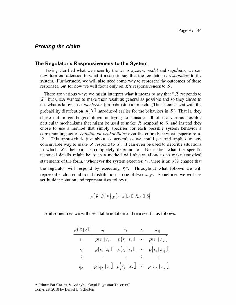
The Regulator's Responsiveness to the SystemHaving clarified what we mean by the terms system, model and regulator, we can
now turn our attention to what it means to say that the regulator is responding to the system. Furthermore, we will also need some way to represent the outcomes of these responses, but for now we will focus only on R 's responsiveness to S .
There are various ways we might interpret what it means to say that “ R responds to S ” but C&A wanted to make their result as general as possible and so they chose to use what is known as a stochastic (probabilistic) approach. (This is consistent with the probability distribution ( )p S introduced earlier for the behaviors in S ) That is, they chose not to get bogged down in trying to consider all of the various possible particular mechanisms that might be used to make R respond to S and instead they chose to use a method that simply specifies for each possible system behavior a corresponding set of conditional probabilities over the entire behavioral repertoire of R . This approach is just about as general as we could get and applies to any conceivable way to make R respond to S . It can even be used to describe situations in which R 's behavior is completely determinate. No matter what the specific technical details might be, such a method will always allow us to make statistical statements of the form, “whenever the system executes js , there is an %x chance that the regulator will respond by executing ir ”. Throughout what follows we will represent such a conditional distribution in one of two ways. Sometimes we will use set-builder notation and represent it as follows:
( ) ( ){ }| | : ,p R S p r s r R s S= ∈ ∈
And sometimes we will use a table notation and represent it as follows:
( )( ) ( ) ( )( ) ( ) ( )
( ) ( ) ( )
1 2
1 1 1 1 2 1
2 2 1 2 2 2
1 2
|
| | |
| | |
| | |
L
L
L
M M M M M
L
S
S
S
R R R R S
p R S s s s
r p r s p r s p r s
r p r s p r s p r s
r p r s p r s p r s
A Primer For Conant & Ashby's “Good-Regulator Theorem”Copyright 2010 by Daniel L. Scholten

Page 10 of 44
In either case, for any regulator behavior, say ir R∈ , and any system behavior, say
js S∈ , the number ( )|i jp r s is the conditional probability that the regulator will
respond by executing behavior ir given the condition that the system executes behavior js . Note that in dealing with such conditional distributions it should always be kept in mind that each number in the distribution is between 0 and 1 inclusive and that the sum of the numbers in any column must total 1. More formally, we will write:
( )
( )1
0 | 1, for all and all
and
| 1, for all
i j i j
R
i j ji
p r s r R s S
p r s s S=
≤ ≤ ∈ ∈
= ∈∑
To return to our current example, since there are an infinite number of real numbers between 0 and 1, then clearly there are an infinite number of ways we might create such a conditional distribution in order to specify out regulator’s responsiveness to the system. One (somewhat complicated) example would be the following:
( ) 1 2 3 4 5 6
1
2
3
4
|.20 .45 .50 .85 1.0 .40.30 .19 .21 0.1 0 .310 .19 .19 14.9 0 .14
.50 .17 .10 0 0 .15
p R S s s s s s srrrr
What the above distribution tells us, for example, is that whenever the system executes behavior 1s the regulator will never respond by doing behavior 3r (since
( )3 1| 0p r s = ) but that it will do behavior 4r on roughly half of all such occasions
(since ( )4 1| .50p r s = ), and that it will do behaviors 1r and 2r on roughly 20% and
30% respectively of all such occasions ( ( )1 1| .20p r s = and ( )2 1| .30p r s = ). As another example, the above table tells us that R will execute 1r in response to 85% of the times that the system executes behavior 4s , that R will do 2r and 3r on 0.1% and 14.9% of all such occasions respectively, and that it will never do 4r on such occasions. As a third example, the above schedule tells us that the R will always do
A Primer For Conant & Ashby's “Good-Regulator Theorem”Copyright 2010 by Daniel L. Scholten

Page 11 of 44
1r in response to the system doing 5s and never do any of its other behaviors in such a situation.
Clearly the above distribution fulfills the two conditions for any such conditional distribution. That is, each number in the distribution is between 0 and 1 inclusive, and if you pick any column and sum the numbers in that column you arrive at a total of 1. The meaning of this latter fact is that the regulator’s behavioral repertoire
{ }1 2 3 4, , ,R r r r r= is really a complete inventory of all possible regulator behaviors and since it is a tautology to say that the regulator must always be doing something that it can do then the probability that it does something it can do (given the system has done, say js ) must equal 1. In other words, and since R ’s behaviors are mutually exclusive,
{ }{ }( ) ( ) ( ) ( )
1 2 3 4
1 2 3 4
the regulator does something it can do | the system has done
the regulator does or or or | the system has done
| | | | 1
j
j
j j j j
p s
p r r r r s
p r s p r s p r s p r s
=
= + + + =
Now, the previously displayed conditional distribution represents just one of the infinite number of ways we might set up the regulator R so that it is responsive to S and most of these infinite ways are rather complicated. But there is a much simpler way we might do this. For example, we might use the following distribution:
( ) 1 2 3 4 5 6
1
2
3
4
|0 1 0 0 0 10 0 0 1 0 01 0 1 0 1 00 0 0 0 0 0
p R S s s s s s srrrr
What this much simpler sort of distribution tells us is that whenever the system does some particular behavior, the regulator’s response is always the same. (That should sound familiar, for reasons to be explained shortly). For example, given that the system does, say 1s , then the probability that the regulator does 3r is 1 (that is,
( )3 1| 1p r s = ), meaning that it is certain that the regulator does 3r whenever the system does 1s and that the regulator will never do any other behavior in its repertoire
A Primer For Conant & Ashby's “Good-Regulator Theorem”Copyright 2010 by Daniel L. Scholten
Page 12 of 44
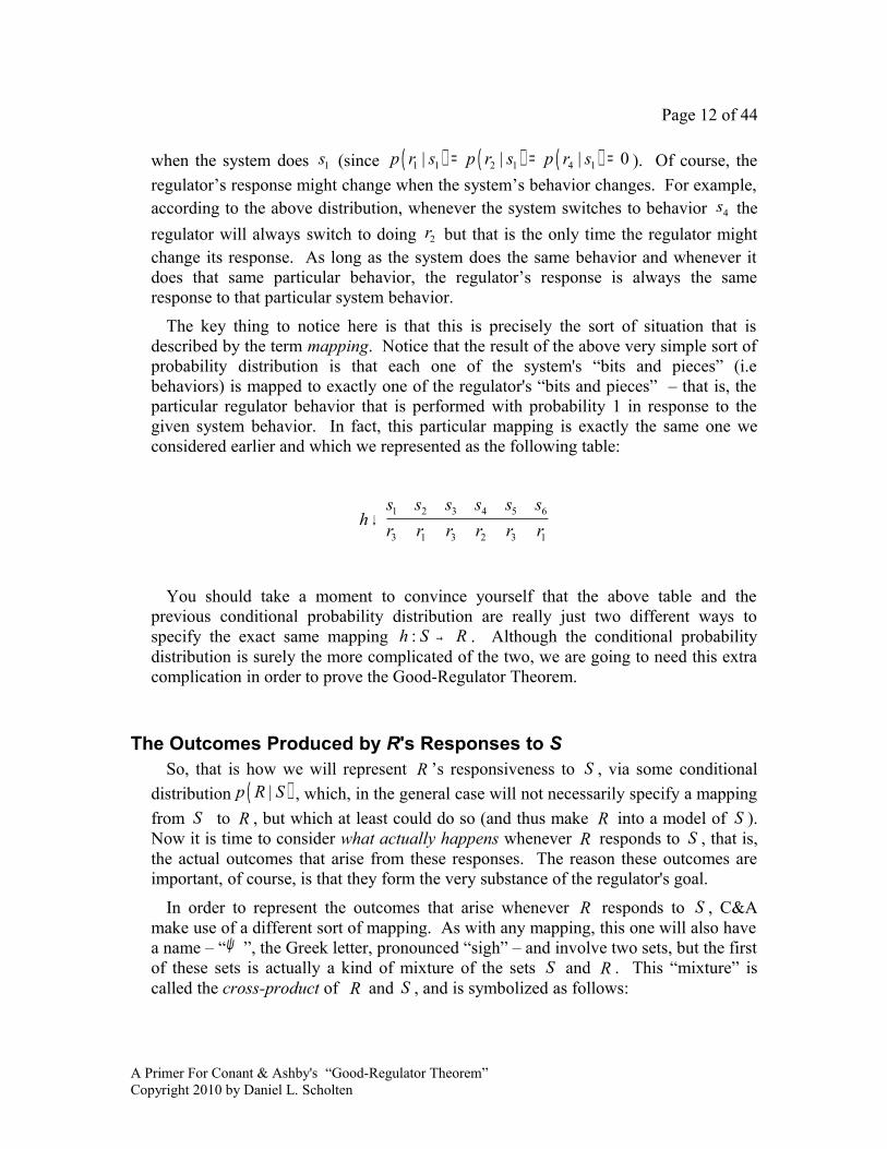
when the system does 1s (since ( ) ( ) ( )1 1 2 1 4 1| | | 0p r s p r s p r s= = = ). Of course, the regulator’s response might change when the system’s behavior changes. For example, according to the above distribution, whenever the system switches to behavior 4s the regulator will always switch to doing 2r but that is the only time the regulator might change its response. As long as the system does the same behavior and whenever it does that same particular behavior, the regulator’s response is always the same response to that particular system behavior.
The key thing to notice here is that this is precisely the sort of situation that is described by the term mapping. Notice that the result of the above very simple sort of probability distribution is that each one of the system's “bits and pieces” (i.e behaviors) is mapped to exactly one of the regulator's “bits and pieces” – that is, the particular regulator behavior that is performed with probability 1 in response to the given system behavior. In fact, this particular mapping is exactly the same one we considered earlier and which we represented as the following table:
1 2 3 4 5 6
3 1 3 2 3 1
s s s s s sh r r r r r r↓
You should take a moment to convince yourself that the above table and the previous conditional probability distribution are really just two different ways to specify the exact same mapping : →h S R . Although the conditional probability distribution is surely the more complicated of the two, we are going to need this extra complication in order to prove the Good-Regulator Theorem.
The Outcomes Produced by R's Responses to SSo, that is how we will represent R ’s responsiveness to S , via some conditional
distribution ( )|p R S , which, in the general case will not necessarily specify a mapping from S to R , but which at least could do so (and thus make R into a model of S ). Now it is time to consider what actually happens whenever R responds to S , that is, the actual outcomes that arise from these responses. The reason these outcomes are important, of course, is that they form the very substance of the regulator's goal.
In order to represent the outcomes that arise whenever R responds to S , C&A make use of a different sort of mapping. As with any mapping, this one will also have a name – “ψ ”, the Greek letter, pronounced “sigh” – and involve two sets, but the first of these sets is actually a kind of mixture of the sets S and R . This “mixture” is called the cross-product of R and S , and is symbolized as follows:
A Primer For Conant & Ashby's “Good-Regulator Theorem”Copyright 2010 by Daniel L. Scholten

Page 13 of 44
The cross-product of R and S = { }, : ,R S r s r R s S× = ∈ ∈
The elements in this set are known as ordered pairs and each ordered pair in that set consists of a single element from the set R along with a single element from the set S. For example, if the element from R is ir and the element from S is js , then we can
symbolize the ordered pair that consists of these two elements as ,i jr s . The cross-product of R and S, then, is the set that consists of every possible such ordered pair.
That describes the first set involved in the mapping we are calling “ψ ”.The second set is just the set of every possible outcome that could arise from some combination of an S behavior and an R behavior. We’re treating the most general case here so we won’t be concerned with any particular details of such outcomes, but
we will introduce a third set { }1 2, , , ZZ z z z= K to represent these possible outcomes.
Thus, the purpose of the mapping ψ is to link each particular combination of a regulator behavior and a system behavior, that is, each ordered pair ,r s R S∈ × , to a unique result or outcome in the set Z . Using the standard shorthand introduced above we can represent this mapping as : R S Zψ × → . (Of course, based on our earlier discussion of models, the existence of this mapping means that we can also say that “Z is a model of ×R S ”, but this particular model is not the one we are really concerned with here and so we will just ignore this option. As it concerns our present discussion of the outcomes that arise from the regulator's responses to the system, we are only interested in the actual mapping : R S Zψ × → .)
Now, if we happen to know, for example that the particular ordered pair ,i jr s R S∈ × maps under ψ to the particular result kz Z∈ , then we could represent
this particular fact as ( ),i j kr s zψ = , or perhaps the more streamlined ( ),i j kr s zψ = ,
as C&A do, which renders the angle brackets “ ” implicit.
To illustrate all of this with a more concrete example, let’s use the sets { }1 2 3 4 5, , , ,R r r r r r= and { }1 2 3 4 5, , , ,S s s s s s= and for the set of possible results we’ll use { }1 2 3 4 5 6 7 8, , , , , , ,Z z z z z z z z z= . The sizes of the sets R and S in this example are a
little different from the ones we used earlier, but these differences are superficial and the only reason I’ve made them different is to illustrate that the differences don’t really matter. One thing we should recognize about these sorts of examples is that they are not meant to imply any restrictions on the sizes of the sets R , S or Z , (represented by R , S and Z , respectively) either in an absolute sense or relative to each other, and in practice any of these, in fact, may be infinite. Thus, although in this example we have that RSZ ==>= 58 this is really just a matter of haphazard
A Primer For Conant & Ashby's “Good-Regulator Theorem”Copyright 2010 by Daniel L. Scholten
Page 14 of 44
convenience. In the general case we might have any of the following: RSZ ≤≤ , SRZ ≤≤ , RZS ≤≤ , ZRS ≤≤ , ZSR ≤≤ or SZR ≤≤ .
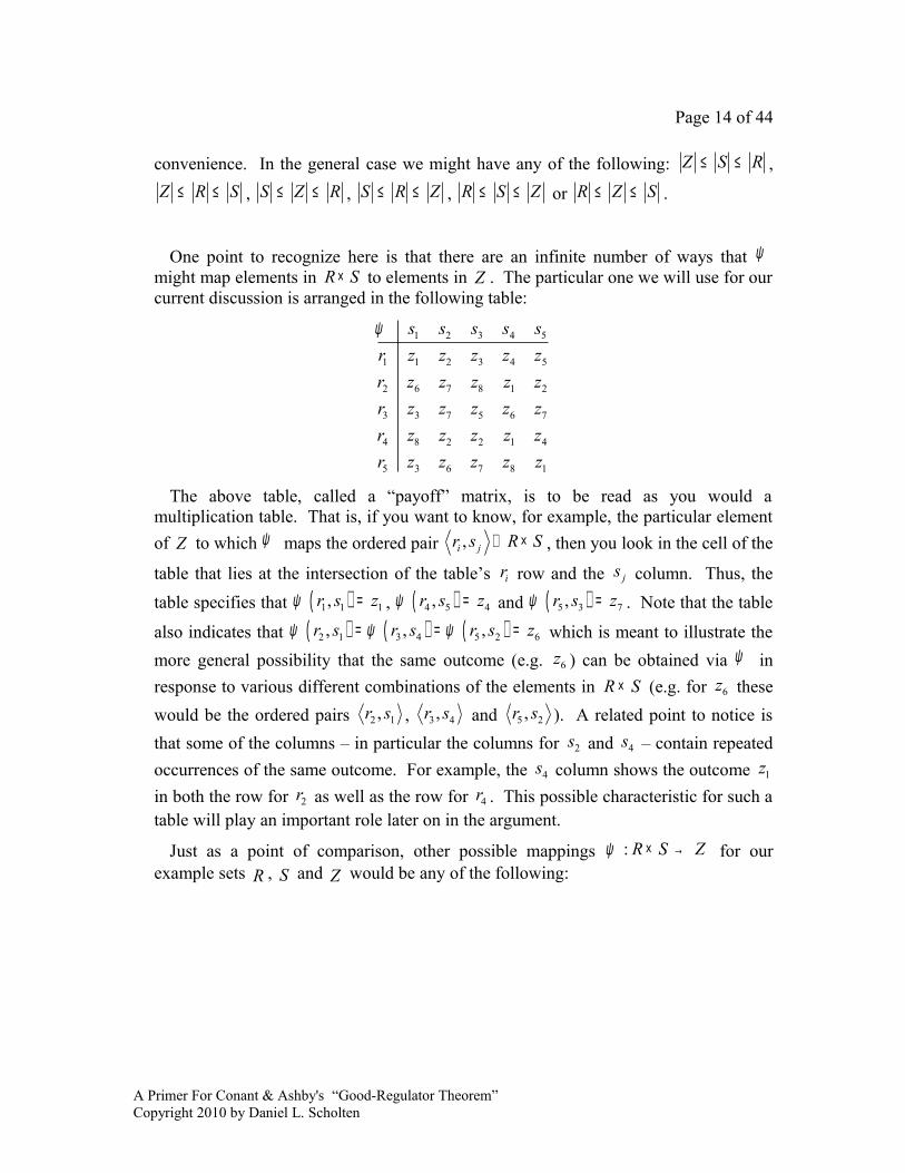
One point to recognize here is that there are an infinite number of ways that ψ might map elements in R S× to elements in Z . The particular one we will use for our current discussion is arranged in the following table:
1 2 3 4 5
1 1 2 3 4 5
2 6 7 8 1 2
3 3 7 5 6 7
4 8 2 2 1 4
5 3 6 7 8 1
s s s s sr z z z z zr z z z z zr z z z z zr z z z z zr z z z z z
ψ
The above table, called a “payoff” matrix, is to be read as you would a multiplication table. That is, if you want to know, for example, the particular element of Z to which ψ maps the ordered pair ,i jr s R S∈ × , then you look in the cell of the
table that lies at the intersection of the table’s ir row and the js column. Thus, the table specifies that ( )1 1 1,r s zψ = , ( )4 5 4,r s zψ = and ( )5 3 7,r s zψ = . Note that the table
also indicates that ( ) ( ) ( )2 1 3 4 5 2 6, , ,r s r s r s zψ ψ ψ= = = which is meant to illustrate the more general possibility that the same outcome (e.g. 6z ) can be obtained via ψ in response to various different combinations of the elements in SR × (e.g. for 6z these would be the ordered pairs 2 1,r s , 3 4,r s and 5 2,r s ). A related point to notice is that some of the columns – in particular the columns for 2s and 4s – contain repeated occurrences of the same outcome. For example, the 4s column shows the outcome 1z in both the row for 2r as well as the row for 4r . This possible characteristic for such a table will play an important role later on in the argument.
Just as a point of comparison, other possible mappings ZSR →×:ψ for our example sets R , S and Z would be any of the following:
A Primer For Conant & Ashby's “Good-Regulator Theorem”Copyright 2010 by Daniel L. Scholten

Page 15 of 44
1 2 3 4 5
1 3 2 6 6 1
2 3 7 8 1 2
3 3 8 5 6 7
4 8 2 4 7 4
5 5 6 4 8 1
s s s s sr z z z z zr z z z z zr z z z z zr z z z z zr z z z z z
ψ
1 2 3 4 5
1 4 4 4 4 4
2 4 4 4 4 4
3 4 4 4 4 4
4 4 4 4 4 4
5 4 4 4 4 4
s s s s sr z z z z zr z z z z zr z z z z zr z z z z zr z z z z z
ψ
1 2 3 4 5
1 1 2 3 4 5
2 6 7 8 1 2
3 3 4 5 6 7
4 8 1 2 3 4
5 5 6 7 8 1
s s s s sr z z z z zr z z z z zr z z z z zr z z z z zr z z z z z
ψ
And as an illustration of examples involving different sets R , S and Z consider the following:
1 2 3 4 5 6 7
1 11 4 6 8 3 1 3
2 1 1 3 5 2 7 5
3 10 1 8 5 11 1 6
s s s s s s sr z z z z z z zr z z z z z z zr z z z z z z z
ψ
and
1 2 3 4
1 1 5 11 9
2 14 2 6 8
3 15 1 3 13
4 10 15 1 4
5 8 7 8 12
6 12 6 6 9
s s s sr z z z zr z z z zr z z z zr z z z zr z z z zr z z z z
ψ
Optimal RegulationOnce we have specified a conditional distribution ( )|p R S and the mapping : R S Zψ × → , then we have everything that we need to know both about the
regulator's responsiveness to the system as well as what actually happens as a result of that responsiveness. The next question we have to address concerns what it means to say that a regulator is “optimal”, or, that it is “doing the best-possible job under the given circumstances”. We can also refer to this as “successful regulation”.
In order to define what it means to say that a regulator behaves optimally, let’s start by considering an actual regulator. For example, suppose we want to purchase a thermostat in order to regulate room temperature. How could we tell if a thermostat is a good thermostat? Clearly, a thermostat is successful when it behaves in such a way as to keep the room temperature constant, or as close to constant as possible, especially when the outside temperatures are fluctuating. Generalizing from this example we might conclude that any regulator can be considered successful if it behaves in such a way as to achieve as much constancy or as little change as possible in the set of outcomes it produces. Another way to say this is that a successful regulator should reduce as much as possible the unpredictability in the set of outcomes it produces.
But hold on. Suppose we purchase a thermostat and discover once it is installed that it does a fantastic job of maintaining a constant room temperature, but that the only
A Primer For Conant & Ashby's “Good-Regulator Theorem”Copyright 2010 by Daniel L. Scholten

Page 16 of 44
constant room temperature it maintains is 350°F! Should we still consider this regulator successful? Suppose furthermore that it does such a great job of maintaining the room temperature at 350°F that it could do so even if the room were placed on the surface of the planet Mercury where the outside temperatures range from a low of -300°F to a high of 800°F. Now how should we evaluate the success of this thermostat?
On the one hand, 350°F is a lousy room temperature so we might conclude that the regulator in question is doing a lousy job. On the other hand, any device that could maintain a constant room temperature in the face of such extreme outside temperature variation as is found on the surface of Mercury is a pretty amazing device indeed – regardless of what that constant temperature might be. Furthermore, suppose we actually needed to maintain such a constant 350°F temperature under such extreme conditions. That is, suppose we wanted to open, say, a high volume cupcake factory on the surface of Mercury, where we needed to bake cupcakes at 350°F around the clock all year long. In that albeit bizarre situation such a regulator would be just what the doctor ordered. Under such circumstances, such a regulator would clearly be successful.
The point of this example is to illustrate that regulator success can be defined in at least a couple of ways. On the one hand, we might say that a regulator is successful as long as it can minimize changes in the outcomes it produces, regardless of what those outcomes might be. Such a definition would always count as successful such regulators as the above thermostat. On the other hand, we might add the additional requirement that a regulator should be able to receive some user's arbitrary temperature request – 350°F, 25°F, 118°F, etc. – and then adjust itself so as to maintain that requested temperature. Such a definition would exclude the above thermostat in some situations (if we were planning to use it, say, to regulate living room temperature) and it would include it in others (if we wanted to use it to maintain temperature in a cupcake oven on Mercury).
Presumable because the first approach is more general, and because the second approach depends on the somewhat arbitrary requirements of the context in which the regulator is actually used, Conant and Ashby use the first approach. That is, they define regulator success strictly in terms of stability – the minimization of the changes in the outcomes produced by the regulator's responses to the system. If it turns out that a given regulator produces a constant (or relatively constant) set of outcomes that happen to be undesirable in one context, well, then that just means we have to find the right context for the regulator, but we will still count it as a good regulator.
Next we need a way to measure the extent to which the regulator is able to achieve such a set of (relatively) constant outcomes. Now, if the outcomes are associated with some numeric variable, such as temperature in the case of a thermostat, then the standard measuring tool would be the statistical variance which is defined as the expected value of the squared differences between the outcomes obtained and the expected value of those outcomes. Formally, letting X represent the numeric variable
A Primer For Conant & Ashby's “Good-Regulator Theorem”Copyright 2010 by Daniel L. Scholten

Page 17 of 44
associated with the outcome, and letting ( )E X represent the expected value of X , then the variance of X is defined as,
( ) ( )( ) 2Var X E X E X = −
But this approach requires that we have some numeric variable we can measure and Conant and Ashby wanted to treat those cases as well as cases in which no such numeric variable was available. In order to accomplish this they use a device from Information Theory called the Shannon Entropy Function which is basically a measure of variation that depends only on the probability distribution that governs whatever particular process whose variation we are trying to measure. In the current context the process that concerns us involves the occurrences of the various outcomes in Z that result from combining regulator behaviors with system behaviors and so, letting
( )kp z represent the probability that some particular result kz Z∈ is obtained, the
probability distribution of interest is ( ) ( ) ( ){ }1 2( ) , , ,= K Zp Z p z p z p z and the
entropy function for the set Z of outcomes is defined as follows:
( ) ( ) ( )1
logZ
k kk
H Z p z p z=
≡ − ∑
Thus, C&A define an optimal regulator as one that responds to the system so as to make the entropy ( )H Z as small as possible, given R , S , Z , ( )p S and
: R S Zψ × → . Notice that in that definition the only variable not assumed given is the conditional distribution ( )|p R S which specifies the regulator’s responsiveness to the system. The reason for this is that, in our present context, the whole point of regulator design is the specification of this conditional probability distribution. That is, we are assuming that we, as regulator designers, have total control over choosing this distribution in our search for an optimal regulator and also that this is really the only thing we can control. In other words, we are assuming that someone has plunked down onto our workbench some system with a behavioral repertoire S and an associated probability distribution ( )p S , along with some regulator with a behavioral repertoire R , a set of possible results Z , and a mapping : R S Zψ × → , and that we have been asked to find a way to make R responsive to S – that is, to design a conditional distribution ( )|p R S – in such a way as to minimize the associated value
of the entropy function ( )H Z . Of course, this raises the question as to how we are supposed to accomplish this. We will return to this question shortly.
A Primer For Conant & Ashby's “Good-Regulator Theorem”Copyright 2010 by Daniel L. Scholten

Page 18 of 44
Actually, C&A make an additional implicit assumption which I want to go ahead and make explicit. It’s a small but important detail, and I want to get it out of the way. This assumption is that the system’s behavioral repertoire only contains behaviors that the system actually might perform. Another way to say this is that S is such that every probability in ( )p S is greater than zero. This is easy enough to do. If we start off with some version of S that contains a behavior, say sα , that cannot occur, that is, which is such that ( ) 0p sα = , then we can just create a new version of S from which sα has been excluded. Since sα could never occur anyway, its exclusion from S has no impact beyond making every probability in ( )p S greater than zero and this is
necessary if we want to define ( )|p R S without having to resort to any special notational gymnastics, and that’s why I want to make this assumption explicit.
A “Useful and Fundamental Property of the Entropy Function”
Generally speaking, the entropy function has a number of properties that make it a useful measure of unpredictability. First of all, for an arbitrary process with event
repertoire { }1 2, , , XX x x x= K the entropy function ( )H X can take on values that
range between an absolute minimum of ( ) 0H X = and an absolute maximum of( ) logH X X= . When ( ) 0H X = then the process is said to be completely
predictable and when ( ) logH X X= the process is said to be completely
unpredictable. A situation in which ( )0 logH X X< < is somewhere between these two extremes.
The entropy function has another attribute that we will need shortly. The authors describe this characteristic of the entropy function as a “useful and fundamental property” which is that if we pick any two probabilities used to calculate the entropy, and we then increase the imbalance between those two probabilities, that is, if we make the bigger one even bigger and the smaller one even smaller, and then if we recalculate the entropy using these new probabilities, then the recalculated entropy will be smaller than the original entropy.
I am going to use a little basic calculus now to prove that this property holds, but if you aren't comfortable with calculus you can just skip this next part and take it on faith that this truly is a property of the entropy function. If you are comfortable with calculus, the argument proceeds as follows.
A Primer For Conant & Ashby's “Good-Regulator Theorem”Copyright 2010 by Daniel L. Scholten

Page 19 of 44
First of all we start with any set of numbers, say 1 2, ,..., np p p , where each is assumed to be between 0 and 1 inclusive, and then we choose any two of them, say ap and bp , where we can assume, without loss of generality, that a bp p≥ (otherwise we just re-label them). Then we choose any positive number δ , where 10 << δ , such that 1 0a a b bp p p pδ δ≥ + > ≥ > − ≥ (which actually implies that 0 bpδ< < ). Then the claim we wish to prove is the following:
( ) ( )1 2 1 2, ,..., ,..., ,... , ,..., ,..., ,...a b n a b nH p p p p p H p p p p pδ δ+ − <
In order to prove this result, we hold constant the 1 2, ,..., np p p and define the following function ( )H δ , where 0 bpδ≤ < ,
( ) ( )
( ) ( ) ( ) ( )1 2
1,,
, ,..., ,..., ,...
log log log
a b n
n
a a b b i iii ai b
H H p p p p p
p p p p p p
δ δ δ
δ δ δ δ=≠≠
= + −
= − + + − − − − ∑
Notice that when 0=δ , this function ( )H δ is equal to the original entropy of
( ) ( ) ( )1 2 1 20 , ,..., 0,..., 0,... , ,..., ,..., ,...a b n a b nH H p p p p p H p p p p p= + − =
Next, still holding constant the 1 2, ,..., np p p , we take the derivative of ( )H δ with respect toδ :
( )( ) ( ) ( )
( ) ( )
( ) ( )
( )( )
( 1)log ( 1) log
1 log 1 log
log
a ba b
a b
a b
b
a
p pdH p pd p p
p p
pp
δ δδ δ
δ δ δ
δ δ
δδ
− + − − −= − + + − − −
+ −
= − − + + + −
−=
+
Now we observe that 0<δd
dH for any δ such that 0 bpδ< < . How do we know
this? Well, first of all, remember that we assumed that a bp p≥ and so 0 bpδ< <
A Primer For Conant & Ashby's “Good-Regulator Theorem”Copyright 2010 by Daniel L. Scholten

Page 20 of 44
implies that a bp pδ δ+ > − and thus that 1b
a
pp
δδ
− <+ and since the logarithm function
is strictly increasing over its entire domain we can conclude that
log log1 0b
a
pdHd p
δδ δ
−= < = + . The fact that 0<
δddH
when 0 bpδ< < means that the
function H is strictly decreasing on the interval 0 bpδ< < which means that
( ) ( )( )( )
1 2
1 2
1 2
, ,..., ,..., ,...
, ,..., ,..., ,...
, ,..., 0,..., 0,... (0)
a b n
a b n
a b n
H H p p p p p
H p p p p p
H p p p p pH
δ δ δ= + −
<
= + −=
.
The important thing to notice in all of that is the following fact:
( ) ( )1 2 1 2, ,..., ,..., ,... , ,..., ,..., ,...
a b n a b nH p p p p p H p p p p pδ δ+ − <
Assuming always, of course, that 0 bpδ< < and that a bp p≥ , as stated earlier, meaning, as claimed, that if we increase the imbalance between any two probabilities, we cause a decrease in the entropy.
Expressing H(Z) in terms of P(R|S)Let's get back to the question we asked a few pages ago. That is, how are we
supposed to find a conditional distribution ( )|p R S that will minimize ( )H Z , given the various above mentioned assumptions? Well, the first thing we need in order to answer this question is some way of relating the entropy function to the conditional distribution ( )|p R S . We will now derive this relationship, but in order to guide our derivation and to make it a bit more concrete we will use the particular example we have already been using. That is, we will use the following for R , S , Z , ( )p S and
ZSR →×:ψ :
{ }1 2 3 4 5, , , ,R r r r r r=
{ }1 2 3 4 5, , , ,S s s s s s=
A Primer For Conant & Ashby's “Good-Regulator Theorem”Copyright 2010 by Daniel L. Scholten

Page 21 of 44
{ }1 2 3 4 5 6 7 8, , , , , , ,Z z z z z z z z z=
( ) ( ) ( ) ( ) ( ) ( ){ }1 2 3 4 5, , , ,p S p s p s p s p s p s=
1 2 3 4 5
1 1 2 3 4 5
2 6 7 8 1 2
3 3 7 5 6 7
4 8 2 2 1 4
5 3 6 7 8 1
s s s s sr z z z z zr z z z z zr z z z z zr z z z z zr z z z z z
ψ
Now, as mentioned earlier on, once any regulator has been built to exhibit the various behaviors in R , be it an optimal regulator or otherwise, the act of setting it up to respond to that system corresponds to the specification of the conditional probability distribution ( )|p R S which we can reproduce in its general form as it applies to our example as follows:
( )( ) ( ) ( ) ( ) ( )( ) ( ) ( ) ( ) ( )( ) ( ) ( ) ( ) ( )( ) ( ) ( ) ( ) ( )( ) ( ) ( ) ( ) ( )
1 2 3 4 5
1 1 1 1 2 1 3 1 4 1 5
2 2 1 2 2 2 3 2 4 2 5
3 3 1 3 2 3 3 3 4 3 5
4 4 1 4 2 4 3 4 4 4 5
5 5 1 5 2 5 3 5 4 5 5
|| | | | || | | | || | | | || | | | || | | | |
p R S s s s s sr p r s p r s p r s p r s p r sr p r s p r s p r s p r s p r sr p r s p r s p r s p r s p r sr p r s p r s p r s p r s p r sr p r s p r s p r s p r s p r s
Remember that each entry ( )|i jp r s in the table represents a number that is understood to be the conditional probability that the regulator responds to an occurrence of js S∈ with the response ir R∈ . Remember also that because these are probabilities, each must be a number between zero and one, and because they are conditional probabilities (each being conditioned on a particular column) we require that the sum of the numbers in any given column must equal exactly one. More formally, we can write:
( )0 | 1i jp r s≤ ≤ , for each 1,2, ,i R= K , and 1,2, ,j S= K ; and
( ) ( ) ( ) ( )1 21
| | | | 1R
i j j j jRi
p r s p r s p r s p r s=
= + + + =∑ L , for each 1,2, ,j S= K .
Of course, for our particular example we have that 5=S and 5=R .
A Primer For Conant & Ashby's “Good-Regulator Theorem”Copyright 2010 by Daniel L. Scholten

Page 22 of 44
Now, as it concerns our particular example, one of the infinite ways we might assign actual numbers to this distribution is as we did earlier:
( ) 1 2 3 4 5
1
2
3
4
5
|.01 .05 0 0 .25.08 .09 0 .50 .39.60 .15 0 .50 .06.25 .40 1 0 0.06 .31 0 0 .30
p R S s s s s srrrrr
One important property to notice about such conditional probability distributions that we will make use of a little later on is that as long as we respect the two basic conditions (that each number in the table is between zero and one and that the numbers in any column sum to one) then we are free to take any valid such distribution
( )|p R S and play around with any one of its columns in any way we like to create a
different distribution, say ( )|p R S′ , that is equally valid. Using our example above, we can, for example, change its third column as shown here:
1 2 3 4 5
1
2
3
4
5
( | ).01 .05 .26 0 .25.08 .09 .2 .50 .39.60 .15 .15 .50 .06.25 .40 .15 0 0.06 .31 .42 0 .30
p R S s s s s srrrrr
′
And the resulting distribution, which I’ve called ( )|p R S′ , is equally valid, meaning that it still respects the two basic conditions. The point here is that whenever we change a column in such a table, we only have to worry about the numbers in that particular column. Another way to say this is that each column is independent of the other columns.
Now, with the distribution ( )p S assumed given, the specification of the conditional
distribution ( )|p R S determines the joint distribution ( ),p R S , since for any js S∈ and ir R∈ we have that the probability that both of these occur together is
( , ) ( ) ( | )i j j i jp r s p s p r s= for each 1,2, ,i R= K , and 1,2, ,j S= K . For our particular example, we can represent this joint probability distribution for R and S in its most general form as follows:
A Primer For Conant & Ashby's “Good-Regulator Theorem”Copyright 2010 by Daniel L. Scholten

Page 23 of 44
( )( ) ( ) ( ) ( ) ( )( ) ( ) ( ) ( ) ( )( ) ( ) ( ) ( ) ( )( ) ( ) ( ) ( ) ( )( ) ( ) ( ) ( ) ( )
1 2 3 4 5
1 1 1 1 2 1 3 1 4 1 5
2 2 1 2 2 2 3 2 4 2 5
3 3 1 3 2 3 3 3 4 3 5
4 4 1 4 2 4 3 4 4 4 5
5 5 1 5 2 5 3 5 4 5 5
,, , , , ,, , , , ,, , , , ,, , , , ,, , , , ,
p R S s s s s sr p r s p r s p r s p r s p r sr p r s p r s p r s p r s p r sr p r s p r s p r s p r s p r sr p r s p r s p r s p r s p r sr p r s p r s p r s p r s p r s
But the specification of ( )|p R S also determines the probability distribution
( ) ( ) ( ) ( ){ }1 2, , , Zp Z p z p z p z= K and thus the entropy function for ( )H Z .
How so? To see this, let’s consider our example. Take another look at the table for our example mapping ZSR →×:ψ , which I’ll reproduce here:
1 2 3 4 5
1 1 2 3 4 5
2 6 7 8 1 2
3 3 7 5 6 7
4 8 2 2 1 4
5 3 6 7 8 1
s s s s sr z z z z zr z z z z zr z z z z zr z z z z zr z z z z z
ψ
Notice that in this table, the element 6z appears three times; once each in the columns 1s , 2s and 4s . That is, 2 1 3 4 5 2 6( , ) ( , ) ( , )r s r s r s zψ ψ ψ= = = . Given this information along with the probabilities in the joint distribution ( ),p R S , we can calculate 6( )p z , the probability of the outcome 6z . In order to calculate 6( )p z we first recognize that each of the js S∈ are mutually exclusive as are each of the ir R∈ which means that each of the events { }2 1,r s , { }3 4,r s and { }5 2,r s are also mutually
exclusive. Furthermore, the event { }6z occurs if and only if any one of the mutually
exclusive events { }2 1,r s , { }3 4,r s or { }5 2,r s occurs. And this means that we can calculate 6( )p z as the simple sum of each of the probabilities 2 1( , )p r s , 3 4( , )p r s and
5 2( , )p r s . That is,
6 2 1 3 4 5 2( ) ( , ) ( , ) ( , )p z p r s p r s p r s= + +
A Primer For Conant & Ashby's “Good-Regulator Theorem”Copyright 2010 by Daniel L. Scholten

Page 24 of 44
Reasoning in the same way for each of the elements of Z yields the following for the distribution ( )p Z :
( )
( ) ( ) ( ) ( ) ( )( ) ( ) ( ) ( ) ( )( ) ( ) ( ) ( )( ) ( ) ( )( ) ( ) ( )( ) ( ) ( ) ( )( ) ( ) ( ) ( ) ( )( ) ( )
1 1 1 2 4 4 4 5 5
2 1 2 2 5 4 2 4 3
3 1 3 3 1 5 1
4 1 4 4 5
5 1 5 3 3
6 2 1 3 4 5 2
7 2 2 3 2 3 5 5 3
8 2 3 4
, , , , ,
, , , , ,
, , , ,
, , ,
, , ,
, , , ,
, , , , ,
, ,
p z p r s p r s p r s p r s
p z p r s p r s p r s p r s
p z p r s p r s p r s
p z p r s p r sp Z
p z p r s p r s
p z p r s p r s p r s
p z p r s p r s p r s p r s
p z p r s p r
= + + +
= + + +
= + +
= +=
= +
= + +
= + + +
= + ( ) ( )1 5 4,s p r s
+
Now, equipped with this probability distribution for the elements of Z, we can now calculate the entropy of Z for our particular example as follows:
( ) ( ) ( ) ( ) ( ) ( ) ( )
( ) ( ) ( ) ( ) ( ) ( ) ( ) ( )( ) ( ) ( ) ( ) ( ) ( ) ( ) ( )( ) ( ) ( )
8
1 1 8 81
1 1 2 4 4 4 5 5 1 1 2 4 4 4 5 5
1 2 2 5 4 2 4 3 1 2 2 5 4 2 4 3
1 3 3 1 5 1
log log log
, , , , log , , , ,
, , , , log , , , ,
, , ,
k kk
H Z p z p z p z p z p z p z
p r s p r s p r s p r s p r s p r s p r s p r s
p r s p r s p r s p r s p r s p r s p r s p r s
p r s p r s p r s
=
= − = − − −
= − + + + + + + − + + + + + + − + +
∑ L
( ) ( ) ( )( ) ( ) ( ) ( )( ) ( ) ( ) ( )( ) ( ) ( ) ( ) ( ) ( )( ) ( ) ( ) ( )
1 3 3 1 5 1
1 4 4 5 1 4 4 5
1 5 3 3 1 5 3 3
2 1 3 4 5 2 2 1 3 4 5 2
2 2 3 2 3 5 5 3
log , , ,
, , log , ,
, , log , ,
, , , log , , ,
, , , , lo
p r s p r s p r s
p r s p r s p r s p r s
p r s p r s p r s p r s
p r s p r s p r s p r s p r s p r s
p r s p r s p r s p r s
+ + − + + − + + − + + + + − + + + ( ) ( ) ( ) ( )
( ) ( ) ( ) ( ) ( ) ( )2 2 3 2 3 5 5 3
2 3 4 1 5 4 2 3 4 1 5 4
g , , , ,
, , , log , , ,
p r s p r s p r s p r s
p r s p r s p r s p r s p r s p r s
+ + + − + + + +
It will be useful later to be able to write these equations out for the general case. The problem is that we cannot predict which of the ( ),i jp r s will find their way into
A Primer For Conant & Ashby's “Good-Regulator Theorem”Copyright 2010 by Daniel L. Scholten

Page 25 of 44
the summation for a given ( )kp z and so we cannot use the standard index method to represent the summation. That is, in the general case, we cannot write anything like the following:
( ) ( )1 1
,M N
k i jj i
p z p r s= =
= ∑ ∑
However, one way around this is as follows:
( ) ( )( )1
,k
kz
p z p r sψ −
= ∑
Where ( )1kzψ − is the set of all and only those ordered pairs ,r s R S∈ × that map
to kz Z∈ under ψ . More formally, ( ) ( ){ }1 , : ,k kz r s R S r s zψ ψ− ≡ ∈ × = .
Furthermore, if want to indicate that we are only summing the joint probabilities for, say, the particular column js , we can use the following notational device:
( ) ( )( )1
,s kj
k jz
p z p r sψ −
= ∑
Where ( )1js kzψ − is the set of all and only those ordered pairs , jr s R S∈ × that map
to kz Z∈ under ψ , for some particular js S∈ . More formally,
( ) ( ){ }1 , : ,js k j j kz r s R S r s zψ ψ− ≡ ∈ × = . Note that for any two distinct ,j hs s S∈ , the
sets ( )1js kzψ − and ( )1
hs kzψ − are mutually exclusive. Also, the union of all such sets
over S is just the set ( )1kzψ − . Putting this formally, we have
( ) ( ) ( ) ( ) ( )1 2
1 1 1 1 1
1jS
S
k s k s k s k s kj
z z z z zψ ψ ψ ψ ψ− − − − −
=
= ∪ ∪ ∪ =L U
Using this latter notation we can now write ( )kp z as a double sum using a hybrid indexing style as follows:
A Primer For Conant & Ashby's “Good-Regulator Theorem”Copyright 2010 by Daniel L. Scholten

Page 26 of 44
( ) ( )( )11
,s kj
S
k jj z
p z p r sψ −=
= ∑ ∑
This notation allows us to write ( )kp z in terms of the conditional distribution ( )|p R S as follows:
( ) ( )( )
( ) ( )( )( )
( ) ( )( )
1 1
1
1 1
1
, ,
|
s k s kj j
s kj
S Sj
k j jj jz z j
S
j jj z
p sp z p r s p r s
p s
p s p r s
ψ ψ
ψ
− −
−
= =
=
= =
=
∑ ∑ ∑ ∑
∑ ∑
Let’s take another look at that last expression. In particular, let’s focus on the expression used in the inner sum:
( )( )1
|s kj
jz
p r sψ −
∑
The first thing to realize about this expression is that it is the conditional probability that the regulator produces the outcome kz in response to js S∈ . That is,
( ) ( )( )1
| |s kj
j k jz
p r s p z sψ −
=∑
Secondly, in the general case, and for every js S∈ , this quantity is always between zero and one (inclusively). That is,
( ) ( )( )1
0 | | 1s kj
j k jz
p r s p z sψ −
≤ = ≤∑
A Primer For Conant & Ashby's “Good-Regulator Theorem”Copyright 2010 by Daniel L. Scholten
Page 27 of 44
Thirdly, for any particular js S∈ , it may be the case either that there are no
occurrences of kz in the js column in which case ( )1js kzψ − = ∅ or that for every
occurrence of kz in the js column ( )| 0jp r s = . If either of these is true then we
would have, for that particular js ,
( ) ( )( )1
| | 0s kj
j k jz
p r s p z sψ −
= =∑
And fourth, again for any particular js S∈ , it may be the case that kz is the only
outcome in the js column for which ( )| 0jp r s > . When this is true then we would
have, for that particular js ,
( ) ( )( )1
| | 1s kj
j k jz
p r s p z sψ −
= =∑
To illustrate all of this with our particular example we would have the following sets for ( )1
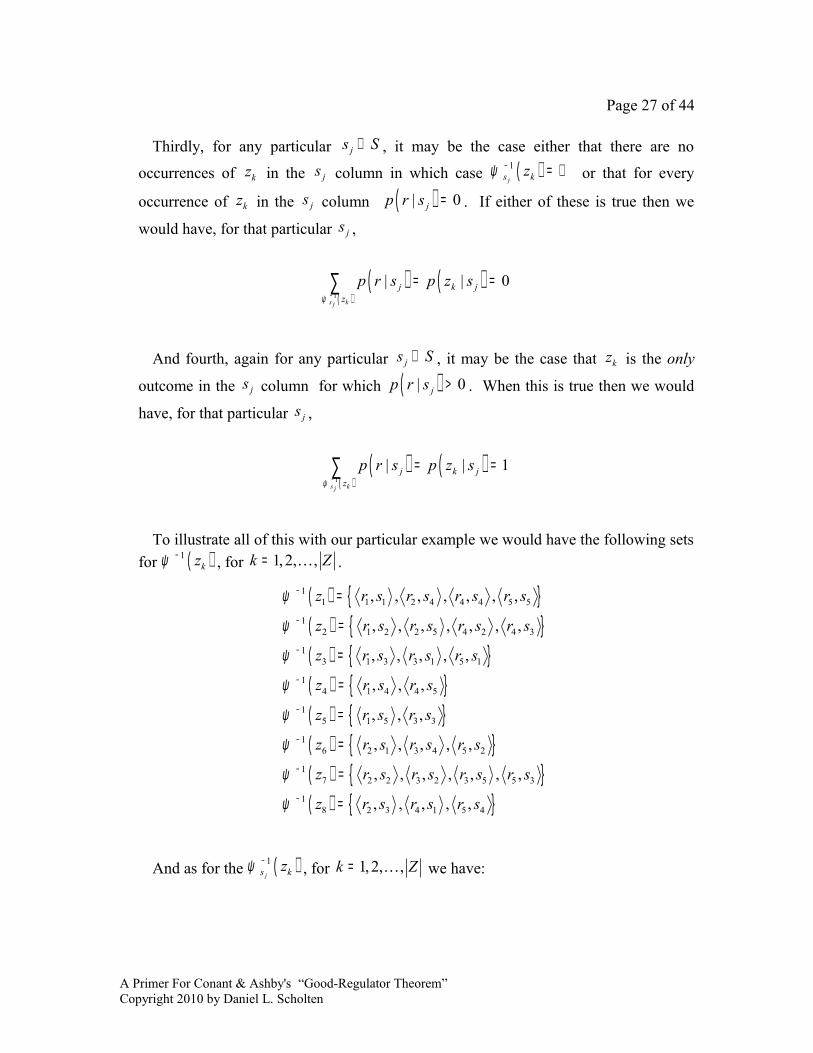
kzψ − , for 1, 2, ,k Z= K .
( ) { }( ) { }( ) { }( ) { }( ) { }( ) { }( ) { }( ) { }
11 1 1 2 4 4 4 5 5
12 1 2 2 5 4 2 4 3
13 1 3 3 1 5 1
14 1 4 4 5
15 1 5 3 3
16 2 1 3 4 5 2
17 2 2 3 2 3 5 5 3
18 2 3 4 1 5 4
, , , , , , ,
, , , , , , ,
, , , , ,
, , ,
, , ,
, , , , ,
, , , , , , ,
, , , , ,
z r s r s r s r s
z r s r s r s r s
z r s r s r s
z r s r s
z r s r s
z r s r s r s
z r s r s r s r s
z r s r s r s
ψ
ψ
ψ
ψ
ψ
ψ
ψ
ψ
−
−
−
−
−
−
−
−
=
=
=
=
=
=
=
=
And as for the ( )1js kzψ − , for 1, 2, ,k Z= K we have:
A Primer For Conant & Ashby's “Good-Regulator Theorem”Copyright 2010 by Daniel L. Scholten

Page 28 of 44
( ) { }( ) { }( ) { }( ) { }( ) { }
1
2
3
4
5
11 1 1
11
11
11 2 4 4 4
11 5 5
,
, , ,
,
s
s
s
s
s
z r s
z
z
z r s r s
z r s
ψ
ψ
ψ
ψ
ψ
−
−
−
−
−
=
=
=
=
=
( ) { }( ) { }( ) { }( ) { }( ) { }
1
2
3
4
5
12
12 1 2 4 2
12 4 3
12
12 2 5
, , ,
,
,
s
s
s
s
s
z
z r s r s
z r s
z
z r s
ψ
ψ
ψ
ψ
ψ
−
−
−
−
−
=
=
=
=
=
( ) { }( ) { }( ) { }( ) { }( ) { }
1
2
3
4
5
13 3 1 5 1
13
13 1 3
13
13
, , ,
,
s
s
s
s
s
z r s r s
z
z r s
z
z
ψ
ψ
ψ
ψ
ψ
−
−
−
−
−
=
=
=
=
=
( ) { }( ) { }( ) { }( ) { }( ) { }
1
2
3
4
5
14
14
14
14 1 4
14 4 5
,
,
s
s
s
s
s
z
z
z
z r s
z r s
ψ
ψ
ψ
ψ
ψ
−
−
−
−
−
=
=
=
=
=
( ) { }( ) { }( ) { }( ) { }( ) { }
1
2
3
4
5
15
15
15 3 3
15
15 1 5
,
,
s
s
s
s
s
z
z
z r s
z
z r s
ψ
ψ
ψ
ψ
ψ
−
−
−
−
−
=
=
=
=
=
( ) { }( ) { }( ) { }( ) { }( ) { }
1
2
3
4
5
16 2 1
16 5 2
16
16 3 4
16
,
,
,
s
s
s
s
s
z r s
z r s
z
z r s
z
ψ
ψ
ψ
ψ
ψ
−
−
−
−
−
=
=
=
=
=
( ) { }( ) { }( ) { }( ) { }( ) { }
1
2
3
4
5
17
17 2 2 3 2
17 5 3
17
17 3 5
, , ,
,
,
s
s
s
s
s
z
z r s r s
z r s
z
z r s
ψ
ψ
ψ
ψ
ψ
−
−
−
−
−
=
=
=
=
=
( ) { }( ) { }( ) { }( ) { }( ) { }
1
2
3
4
5
18 4 1
18
18 2 3
18 5 4
18
,
,
,
s
s
s
s
s
z r s
z
z r s
z r s
z
ψ
ψ
ψ
ψ
ψ
−
−
−
−
−
=
=
=
=
=
Equipped with these more compact notational devices we can write the general form of the entropy function in terms of both the joint distribution ( ),p R S and the
conditional distribution ( )|p R S as follows:
A Primer For Conant & Ashby's “Good-Regulator Theorem”Copyright 2010 by Daniel L. Scholten

Page 29 of 44
( ) ( ) ( ) ( )( )
( )
( )( )
( )
( ) ( )( )
( )
( ) ( )( )
1 1
1 1
this is this is
1 1
this is this is
1 1
log , log ,
| log |
k k
k k
k
s k s kj j
p z p zZ Z
k kk k z z
p z p z
S S
j j j jj jz z
H Z p z p z p r s p r s
p s p r s p s p r s
ψ ψ
ψ ψ
− −
− −
= =
= =
= − = −
= −
∑ ∑ ∑ ∑
∑ ∑ ∑ ∑
64748 64748
64444744448 ( )
1
k
Z
k =
∑64444744448
Note that this is the general form of the entropy function in terms of ( ),p R S and ( )|p R S not simply the version that pertains to our example. (To obtain the version
that applies to our particular example we would have only to plug in the values 8Z =
, 5R = and 5S = ). And equipped with this expression for the entropy function we
are reading to return to the question of how to go about designing ( )|p R S so that ( )H Z is made as small as possible (given R , S , Z , ( )p S and : R S Zψ × → ).
A Lemma Regarding Successful RegulatorsThe next thing we need to accomplish this is to define, as do C&A, the set π that
contains exactly the sort of conditional probability distributions ( )|p R S that we are
looking for – that is, that make the resulting entropy function ( )H Z as small as possible. Actually, π is not really as simple as that because another point the authors make is that it is possible for two different ( )|p R S distributions, say ( )1 |p R S and
( )2 |p R S to determine two different ( )p Z distributions, say ( )1p Z and ( )2p Z ,
where ( ) ( )1 2p Z p Z≠ , in such a way that the resulting entropies ( )1H Z and ( )2H Z are equal. They claim that to consider this possibility would complicate unnecessarily their proof and so they place the additional restriction on π that each of its members determines (via the given ( )p S and ψ ) the same unique ( )p Z . To make this point
more vivid, let’s call the minimum attainable entropy ( )minH Z . Now, if we discover
that, say, both ( )1 |p R S and ( )2 |p R S achieve ( )minH Z , but that ( )1 |p R S
determines ( )1p Z and that ( )2 |p R S determines ( )2p Z where ( ) ( )1 2p Z p Z≠ , then
what the authors want to do is to exclude from the set π either ( )1 |p R S or ( )2 |p R S
A Primer For Conant & Ashby's “Good-Regulator Theorem”Copyright 2010 by Daniel L. Scholten

Page 30 of 44
Thus, π does not contain all of the distributions ( )|p R S that achieve ( )minH Z .
The specification of π requires that we first pick one of the ( )p Z distributions that
achieves ( )minH Z , and that we include only those ( )|p R S distributions in π that
achieve the chosen ( )p Z distribution that in turn determines ( )minH Z . I would like to examine this simplification in more detail, but not at this point. For now, let’s assume the trick is valid and choose an arbitrary ( )|p R S from π .
Now we come to a result that Conant and Ashby call a lemma and which they describe as the heart of their proof. To put it simply, this lemma tells us that the only way to build an optimal regulator (one that makes ( )H Z minimal) is to make sure that it never acts so as to produces different outcomes on different occasions when confronted with the same system behavior. The way they prove this claim is by the method of contradiction, which means that they start by assuming the contrary claim – that it is possible to build an optimal regulator that might produce different outcomes when confronted on different occasions with the same system behavior – and then they deduce a logical contradiction. The deduction of the logical contradiction under the assumption that the original claim is false proves that the original claim is true. We will now walk through Conant and Ashby’s proof of their lemma.
Perhaps the most difficult thing to understand about this lemma is the symbol-dense mathematically terse way they state what it claims which resembles the following:
Lemma : For an arbitrary ( )|p R S in π and for all js S∈ , the set
( ) ( ){ }, : , 0i j i jr s p r sψ > has only one element.
I think the best way to unpack what this lemma is saying is as I already did in the previous paragraph, but in case the connection isn’t obvious we can start with the following. What the above lemma is claiming, is that provided we are looking at an optimal conditional distribution ( )|p R S π∈ , then for any given system behavior
js S∈ , the conditional distribution ( )| jp R S s= is such that if ( )| 0h jp r s > and
( )| 0i jp r s > for any , , h i h ir r R r r∈ ≠ , then it must be the case that
( ) ( ), ,h j i j kr s r s zψ ψ= = , for some kz Z∈ . In case that is still too abstruse, let’s try walking through it using our specific example. Remember that our goal is to specify the following table:
A Primer For Conant & Ashby's “Good-Regulator Theorem”Copyright 2010 by Daniel L. Scholten

Page 31 of 44
( )( ) ( ) ( ) ( ) ( )( ) ( ) ( ) ( ) ( )( ) ( ) ( ) ( ) ( )( ) ( ) ( ) ( ) ( )( ) ( ) ( ) ( ) ( )
1 2 3 4 5
1 1 1 1 2 1 3 1 4 1 5
2 2 1 2 2 2 3 2 4 2 5
3 3 1 3 2 3 3 3 4 3 5
4 4 1 4 2 4 3 4 4 4 5
5 5 1 5 2 5 3 5 4 5 5
|| | | | || | | | || | | | || | | | || | | | |
p R S s s s s sr p r s p r s p r s p r s p r sr p r s p r s p r s p r s p r sr p r s p r s p r s p r s p r sr p r s p r s p r s p r s p r sr p r s p r s p r s p r s p r s
And that we want to specify this table so that the resulting entropy ( )H Z is at a minimum. Now, suppose we have done just that, so that the above table contains a bunch of numbers, all of which are between 0 and 1 such that the sum of the numbers in any given column equals 1 and that if we use these number to calculate ( )H Z then the number we come up with will be the smallest we could achieve. Now, the lemma is telling us that if we first focus our attention on any of the js S∈ , which we can represent as follows:
( )( )( )( )( )( )
1 1
2 2
3 3
4 4
5 5
|
|
|
|
|
|
j
j
j
j
j
j
p R S s
r p r s
r p r s
r p r s
r p r s
r p r s
L L
L L
L L
L L
L L
L L
And if we then notice that ( )| 0h jp r s > and ( )| 0i jp r s > which we can visualize as follows:
( )
( )
( )
|
| 0
| 0
j
h h j
i i j
p R S s
r p r s
r p r s
>
>
L LM L L L
L L
M L L L
L L
M L L L
A Primer For Conant & Ashby's “Good-Regulator Theorem”Copyright 2010 by Daniel L. Scholten

Page 32 of 44
Then according to the lemma, it must be the case that ( ) ( ), ,h j i j kr s r s zψ ψ= = for
some particular kz Z∈ . That is, our table for ψ must look as follows:
j
h k
i k
s
r z
r z
ψ L LM L M LL L
M L M LL L
M L M L
In other words, and as I explained above, the lemma is telling us that the only way to build an optimal regulator (one that makes ( )H Z minimal) is to make sure that it never produces two different outcomes when confronted with the same js S∈ . That is, given some particular js S∈ , when faced with any two responses, say xr and yr , that might otherwise produce different outcomes, then at least one of them should have a probability of zero; that is, if ( ) ( ), ,x j y jr s r sψ ψ≠ then we better make sure that
either ( | ) 0x jp r s = or ( | ) 0y jp r s = , because otherwise ( )H Z cannot be minimal.
In any case, that’s what the lemma is claiming. And as I said above, the authors use a proof by contradiction to establish this result. That is, they first assume, contrary to what the lemma claims is possible, that there does exist a conditional distribution
( )|p R S π∈ (i.e. that minimizes ( )H Z ) which is such that there exists some js S∈
such that ( )| 0x jp r s > and ( )| 0y jp r s > , for , , x y x yr r R r r∈ ≠ , where the outcomes
under ψ are different, that is, ( ) ( ), ,x j k l y jr s z z r sψ ψ= ≠ = , for some ,k lz z Z∈ . After making this assumption, they then deduce a contradiction, which implies that their assumption could not have been true, which, in turn, implies that the lemma must be true.
The details of the proof are as follows. Let’s review the assumptions. First we are assuming, contrary to what the lemma claims is possible, that there does exist a conditional distribution ( )|p R S π∈ (i.e. that minimizes ( )H Z ) which is such that
there exists some js S∈ such that ( )| 0x jp r s > and ( )| 0y jp r s > , for , , x y x yr r R r r∈ ≠ , where the outcomes under ψ are different, that is,
( ) ( ), ,x j k l y jr s z z r sψ ψ= ≠ = , for some ,k lz z Z∈ .
A Primer For Conant & Ashby's “Good-Regulator Theorem”Copyright 2010 by Daniel L. Scholten

Page 33 of 44
Now, let’s consider ( )kp z and ( )lp z . Using the notation we worked out earlier we can write each of these as simple sums of the probabilities in the distribution of
( ),p R S . That is, we can write
( ) ( )( )
( ) ( )( )
1
1
,
and ,
k
l
kz
lz
p z p r s
p z p r s
ψ
ψ
−
−
=
=
∑
∑
But we are assuming that ( ),x j kr s zψ = and ( ),y j lr s zψ = which means that
( )
( )
1
1
,
and
,
x j k
y j l
r s z
r s z
ψ
ψ
−
−
∈
∈
Therefore we can write
( ) ( ) ( )( )
( ) ( ) ( )( )
1
1
,
,
, ,
and
, ,
k x j
l y j
k x jz r s
l y jz r s
p z p r s p r s
p z p r s p r s
ψ
ψ
−
−
−
−
= +
= +
∑
∑
Where we are using the notation ( )1 ,k x jz r sψ − − to represent the set of all ordered
pairs ,r s R S∈ × such that ( ), kr s zψ = but that excludes the particular ordered pair
,x jr s . Similarly the notation ( )1 ,l y jz r sψ − − represents the set of all ordered pairs
,r s R S∈ × such that ( ), lr s zψ = but that excludes the particular ordered pair
,y jr s . More formally we can write,
A Primer For Conant & Ashby's “Good-Regulator Theorem”Copyright 2010 by Daniel L. Scholten

Page 34 of 44
( ) ( ){ }
( ) ( ){ }
1
1
, , : , , , ,
and
, , : , , , ,
k x j k x j
l y j l y j
z r s r s R S r s z r s r s
z r s r s R S r s z r s r s
ψ ψ
ψ ψ
−
−
− = ∈ × = ≠
− = ∈ × = ≠
.
Because these expressions are a bit bulky, let’s make use of the following symbol substitutions:
( )( )
( )( )
1
1
,
,
( , ),
( , ),
, ,
and ,
k x j
l y j
k x j
l y j
kz r s
lz r s
p p r sp p r s
p r s
p r s
ψ
ψ
ε
ε
−
−
−
−
=
=
=
=
∑
∑
Using these substitutions our expressions for ( )kp z and ( )lp z become,
( )
( )and
k k k
l l l
p z p
p z p
ε
ε
= +
= +
With the above streamlined expressions for ( )kp z and ( )lp z we can now express the entropy function as follows:
( ) ( )( )
( )( )
( )( )
( )( )
( ) ( )
( )( )
( )( )
( )( )
this is this is this is this is
1,,
this is this is this is
log log log
log log
k k l l
k k l
p z p z p z p zZ
k k k k l l l l h hhh kh l
p z p z p z
k k k k l l
H Z p p p p p z p z
p p p
ε ε ε ε
ε ε ε
=≠≠
= − + + − + + −
= − + + − +
∑64748 64748 64748 64748
64748 64748 64748( )
( )this is lp z
l lp ε ρ+ +64748
.
A Primer For Conant & Ashby's “Good-Regulator Theorem”Copyright 2010 by Daniel L. Scholten

Page 35 of 44
Where we have introduced yet another space saving substitution in the above by setting
( ) ( )1,
,
logZ
h hhh kh l
p z p zρ=≠≠
= − ∑
Now, remember, this is supposed to be the smallest possible value for ( )H Z that is
attainable because we are using ( )|p R S π∈ to calculate it. More specifically, we
have used ( )|x jp r s and ( )|y jp r s from ( )|p R S to calculate both ( ),x jp r s and
( ),y jp r s (since ( ) ( ) ( ), |x j j x jp r s p s p r s= and ( ) ( ) ( ), |y j j y jp r s p s p r s= ), which
we then used to calculate each of ( )kp z and ( )lp z . So really, we should write
( ) ( )( )
( )( )
( )( )
( )( )this is this is this is this is
min log logk k l lp z p z p z p z
k k k k l l l lH Z p p p pε ε ε ε ρ= − + + − + + +64748 64748 64748 64748
But now if we first figure out which of kp and lp is bigger and then we increase the imbalance between them by adding some δ such that ( )0 min ,k lp pδ< < to the larger of the two and subtracting the same δ from the smaller of the two then by the useful and fundamental property of the entropy function mentioned above we conclude that the resulting ( )H Z will be yet smaller than ( )minH Z , which is, of course, a contradiction! For example, let’s just assume that k lp p≥ . Then by our useful and fundamental property of the entropy function, we conclude that
( ) ( ) ( ) ( ) ( )( ) ( ) ( ) ( )
min log log
log logk k k k l l l l
k k k k l l l l
H Z p p p p
p p p p
ε ε ε ε ρ
δ ε δ ε δ ε δ ε ρ
= − + + − + + +
> − + + + + − − + − + +.
But this is a contradiction. For the case in which k lp p< then we subtract δ from
kp and add δ to lp in order to obtain the same contradiction. Thus, by assuming that the lemma is false, we derive a logical contradiction, which means that the lemma must be true. That is, for any conditional distribution ( )|p R S π∈ (i.e. that minimizes
( )H Z ) and for any js S∈ , if ( )| 0x jp r s > and ( )| 0y jp r s > , for x yr r≠ , then it must be the case that the overall outcomes are the same, that is, that
A Primer For Conant & Ashby's “Good-Regulator Theorem”Copyright 2010 by Daniel L. Scholten

Page 36 of 44
( ) ( ), ,x j k y jr s z r sψ ψ= = . To summarize this in words, whenever faced with a given
js S∈ , any optimal regulator must always produce the same outcome. Notice that it might produce this identical outcome with different responses, say xr and yr , but it can only use such different responses provided they both map with js under ψ to the same kz Z∈ . Any regulator that responds to some particular js S∈ in such a way as to produce, say, kz Z∈ on some occasions and, say, lz Z∈ on different occasions will not be able to minimize ( )H Z .
The Simplest Optimal RegulatorWhat we have established so far is that an optimal (i.e. maximally successful)
regulator will always produce the same outcome, say kz Z∈ , in response to a given
js S∈ . The only thing left now is to prove that the simplest way to accomplish this is to pick any one of the responses that map with js under ψ to that unique outcome kz and to have the regulator always do that response. For example, if it turns out that the responses , ,w x yr r r R∈ are such that ( )| 0w jp r s > , ( )| 0x jp r s > , ( )| 0y jp r s > and
that ( ) ( ) ( ), , ,w j x j y j kr s r s r s zψ ψ ψ= = = , and of course that ( )H Z is minimized, then
what we should do is to pick any one of these responses, say xr , and set ( )| 1x jp r s = ,
which means, of course, that we have to set ( ) ( )| | 0w j y jp r s p r s= = .
Actually, it’s pretty obvious that this would be the simplest thing to do, provided it doesn’t increase ( )H Z . The authors claim that this won’t happen, but how can we be sure? One approach is as follows. First let’s take an arbitrary kz Z∈ , and express
( )kp z using the notation we developed earlier:
( ) ( ) ( )11 ( )
|s kj
S
k j jj z
p z p s p r sψ −=
= ∑ ∑
Now, let us focus our attention on an arbitrary hs S∈ and separate its term out from the rest of the summation as follows:
A Primer For Conant & Ashby's “Good-Regulator Theorem”Copyright 2010 by Daniel L. Scholten

Page 37 of 44
( ) ( ) ( ) ( ) ( )1 11,( ) ( )
| |s k s kh j
S
k h h j jjz zj h
p z p s p r s p s p r sψ ψ− −=
≠
= +∑ ∑ ∑
Although this much is true for any kz Z∈ and any hs S∈ , let us now consider a more specific case. That is, let us suppose, first of all, that we are looking at an optimal regulator, so that ( )|p R S π∈ . Furthermore, let us also suppose that kz is the particular outcome that our regulator always produces when confronted with hs . Under these conditions, it must be the case that
( )1 ( )
| 1s kh
hz
p r sψ −
=∑
And thus, that
( ) ( ) ( ) ( ) ( )
( ) ( ) ( ) ( )
( ) ( ) ( )
1 1
1
1
1,( ) ( )
1, ( )
1, ( )
| |
1 |
|
s k s kh j
s kj
s kj
S
k h h j jjz zj h
S
h j jj zj h
S
h j jj zj h
p z p s p r s p s p r s
p s p s p r s
p s p s p r s
ψ ψ
ψ
ψ
− −
−
−
=≠
=≠
=≠
= +
= +
= +
∑ ∑ ∑
∑ ∑
∑ ∑
What we have established here is that under the stated conditions ( )kp z is
completely independent of the details of the conditional distribution ( )| hp R s and so
we can re-arrange ( )| hp R s however we wish without having any impact on ( )kp z . The only conditions we have to respect are that we have to make sure that
( )0 | 1i hp r s≤ ≤ for all ir R∈ and also that ( )1
| 1R
i hi
p r s=
=∑ .
Now, the fact that ( )kp z is completely independent of the details of the conditional
distribution ( )| hp R s , along with the fact that the details of ( )| hp R s are completely
independent of the details of all of the other column distributions ( )| jp R s , for all
A Primer For Conant & Ashby's “Good-Regulator Theorem”Copyright 2010 by Daniel L. Scholten
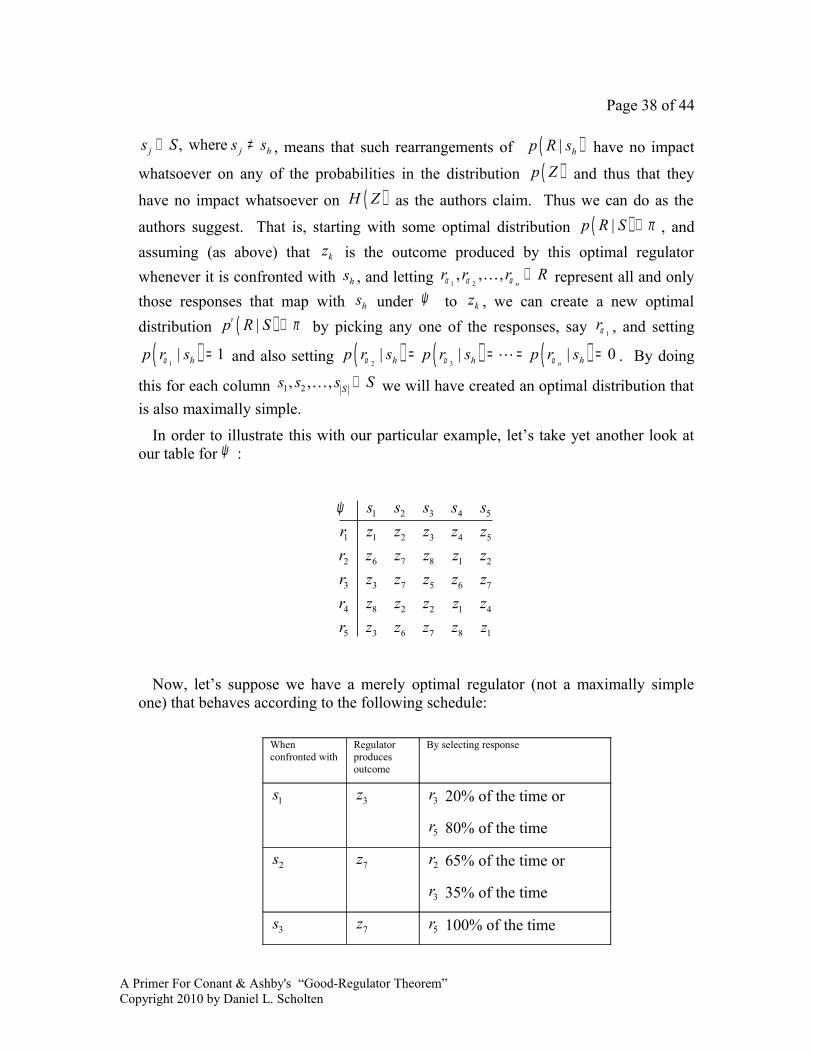
Page 38 of 44
, where j j hs S s s∈ ≠ , means that such rearrangements of ( )| hp R s have no impact
whatsoever on any of the probabilities in the distribution ( )p Z and thus that they
have no impact whatsoever on ( )H Z as the authors claim. Thus we can do as the
authors suggest. That is, starting with some optimal distribution ( )|p R S π∈ , and assuming (as above) that kz is the outcome produced by this optimal regulator whenever it is confronted with hs , and letting 1 2
, , ,n
r r r Rα α α ∈K represent all and only those responses that map with hs under ψ to kz , we can create a new optimal distribution ( )|p R S π′ ∈ by picking any one of the responses, say 1
rα , and setting
( )1| 1hp r sα = and also setting ( ) ( ) ( )2 3
| | | 0nh h hp r s p r s p r sα α α= = = =L . By doing
this for each column 1 2, , , Ss s s S∈K we will have created an optimal distribution that is also maximally simple.
In order to illustrate this with our particular example, let’s take yet another look at our table for ψ :
1 2 3 4 5
1 1 2 3 4 5
2 6 7 8 1 2
3 3 7 5 6 7
4 8 2 2 1 4
5 3 6 7 8 1
s s s s sr z z z z zr z z z z zr z z z z zr z z z z zr z z z z z
ψ
Now, let’s suppose we have a merely optimal regulator (not a maximally simple one) that behaves according to the following schedule:
When confronted with
Regulator produces outcome
By selecting response
1s 3z 3r 20% of the time or
5r 80% of the time
2s 7z 2r 65% of the time or
3r 35% of the time
3s 7z 5r 100% of the time
A Primer For Conant & Ashby's “Good-Regulator Theorem”Copyright 2010 by Daniel L. Scholten

Page 39 of 44
When confronted with
Regulator produces outcome
By selecting response
4s 1z 2r 15% of the time or
4r 85% of the time
5s 7z 3r 100% of the time
Notice that all of the above information can be stored in special hybrid table that combines the tables for ( )|p R S and ψ as follows:
( )1 2 3 4 5
1
27 1
33 7 7
41
53 7
|
0 0 0 0 0.65 .150 0 0
.20 .35 10 0
.850 0 0 0
.80 10 0 0
p R S s s s s s
r
r z z
r z z z
r z
r z z
ψ
Now, if we want to convert this optimal regulator to one that is maximally simple, we just have to fix columns 1s , 2s and 4s so that all of the probability is concentrated on a single response where it really doesn’t matter which response we pick, provided it is one of the responses that already has a positive probability. Let’s just pick response
3r for columns 1s and 2s , and response 4r for column 4s . Now our hybrid table for the maximally simple optimal regulator looks as follows:
A Primer For Conant & Ashby's “Good-Regulator Theorem”Copyright 2010 by Daniel L. Scholten

Page 40 of 44
( )1 2 3 4 5
1
2
33 7 7
41
57
|
0 0 0 0 00 0 0 0 0
1 1 10 0
10 0 0 0
10 0 0 0
p R S s s s s s
rr
r z z z
r z
r z
ψ
Removing the outcome elements from the above table gives us our pure table for the distribution ( )|p R S as follows:
( ) 1 2 3 4 5
1
2
3
4
5
|0 0 0 0 00 0 0 0 01 1 0 0 10 0 0 1 00 0 1 0 0
p R S s s s s srrrrr
And as discussed in the opening of this paper, this sort of distribution ( )|p R S which consists entirely of ones and zeros specifies a mapping :h S R→ . For this current example, the mapping can be represented as follows:
1 2 3 4 5
3 3 5 4 3:S s s s s s
h R r r r r r
A Primer For Conant & Ashby's “Good-Regulator Theorem”Copyright 2010 by Daniel L. Scholten

Page 41 of 44
Conclusion: a “Rigorous Theorem”
Congratulations. If you have made it this far you have successfully understood the proof of Conant and Ashby's Good-Regulator Theorem. In closing I would like to discuss the following assertion that Conant and Ashby make in their paper:
The first effect of this theorem is to change the status of model-making from optional to compulsory. As we said earlier, model-making has hitherto largely been suggested (for regulating complex dynamic systems) as a possibility: the theorem shows that, in a very wide class (specified in the proof of the theorem), success in regulation implies that a sufficiently similar model must have been built, whether it was done explicitly, or simply developed as the regulator was improved. Thus the would be model-maker now has a rigorous theorem to justify his work. [page 97, emphasis added]
This is a strong statement, but it contains some subtlety that needs to be understood. The subtlety revolves around the phrase “whether it was done explicitly, or simply developed as the regulator was improved.” To really see what this entails, let's take another look at the statement of the theorem:
Theorem : The simplest optimal regulator R of a system S produces behaviors
from { }1 2, , , RR r r r= L which are related to the behaviors in
{ }1 2, , SS s s s= L by a mapping : →h S R .
Notice that this statement actually refers to what we can recognize as two distinct models. On the one hand there is the actual regulator device R which is a dynamic entity and which, through its simplest optimal regulation of the system S , comes to be a dynamic model of that system. This is the so-called “good-regulator model” referred to by the title of C&A's paper: every good regulator of a system must be a model of that system. But the statement of the theorem also refers to the mapping : →h S R , which is also a model. More specifically, this mapping is a model of the representational relationship between the good-regulator and the system it regulates. This mapping is a model for the same reason that the good-regulator itself is a model, because there is yet another mapping, call it k , that is set up between the component “bits and pieces” of the regulator/system ensemble and the component “bits and pieces” of the mapping : →h S R . Of course, this mapping we are calling k is just the one we build in our own minds so that we can understand the theorem.
This second model : →h S R is really just a description of the good-regulator model. We can think of it as the “technical specification” of that model. It is a
A Primer For Conant & Ashby's “Good-Regulator Theorem”Copyright 2010 by Daniel L. Scholten
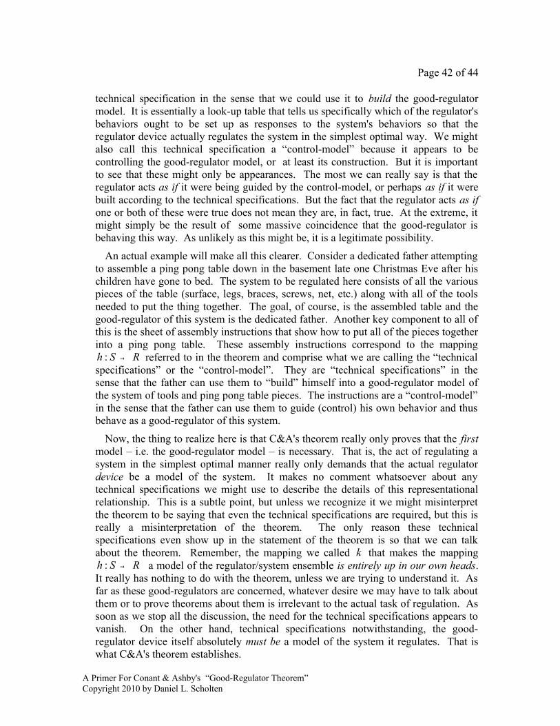
Page 42 of 44
technical specification in the sense that we could use it to build the good-regulator model. It is essentially a look-up table that tells us specifically which of the regulator's behaviors ought to be set up as responses to the system's behaviors so that the regulator device actually regulates the system in the simplest optimal way. We might also call this technical specification a “control-model” because it appears to be controlling the good-regulator model, or at least its construction. But it is important to see that these might only be appearances. The most we can really say is that the regulator acts as if it were being guided by the control-model, or perhaps as if it were built according to the technical specifications. But the fact that the regulator acts as if one or both of these were true does not mean they are, in fact, true. At the extreme, it might simply be the result of some massive coincidence that the good-regulator is behaving this way. As unlikely as this might be, it is a legitimate possibility.
An actual example will make all this clearer. Consider a dedicated father attempting to assemble a ping pong table down in the basement late one Christmas Eve after his children have gone to bed. The system to be regulated here consists of all the various pieces of the table (surface, legs, braces, screws, net, etc.) along with all of the tools needed to put the thing together. The goal, of course, is the assembled table and the good-regulator of this system is the dedicated father. Another key component to all of this is the sheet of assembly instructions that show how to put all of the pieces together into a ping pong table. These assembly instructions correspond to the mapping
: →h S R referred to in the theorem and comprise what we are calling the “technical specifications” or the “control-model”. They are “technical specifications” in the sense that the father can use them to “build” himself into a good-regulator model of the system of tools and ping pong table pieces. The instructions are a “control-model” in the sense that the father can use them to guide (control) his own behavior and thus behave as a good-regulator of this system.
Now, the thing to realize here is that C&A's theorem really only proves that the first model – i.e. the good-regulator model – is necessary. That is, the act of regulating a system in the simplest optimal manner really only demands that the actual regulator device be a model of the system. It makes no comment whatsoever about any technical specifications we might use to describe the details of this representational relationship. This is a subtle point, but unless we recognize it we might misinterpret the theorem to be saying that even the technical specifications are required, but this is really a misinterpretation of the theorem. The only reason these technical specifications even show up in the statement of the theorem is so that we can talk about the theorem. Remember, the mapping we called k that makes the mapping
: →h S R a model of the regulator/system ensemble is entirely up in our own heads. It really has nothing to do with the theorem, unless we are trying to understand it. As far as these good-regulators are concerned, whatever desire we may have to talk about them or to prove theorems about them is irrelevant to the actual task of regulation. As soon as we stop all the discussion, the need for the technical specifications appears to vanish. On the other hand, technical specifications notwithstanding, the good-regulator device itself absolutely must be a model of the system it regulates. That is what C&A's theorem establishes.
A Primer For Conant & Ashby's “Good-Regulator Theorem”Copyright 2010 by Daniel L. Scholten
Page 43 of 44
As these observations relate to our dedicated father, the Good-Regulator Theorem only proves that the father must act as if his behavior were being guided by the assembly instructions. It does not prove that the actual assembly instructions themselves are necessary to the successful assembly of the table. Of course, having observed all of this, it does appear to be a matter of empirical fact that such technical specifications are also necessary, or at least extremely useful. A disciplined glance throughout the world of human behavior reveals that most of what makes modern civilization “modern” would be practically impossible without these sorts of technical specifications. Ping pong table assembly instructions, architectural blueprints, computer software specifications, library catalogs, cooking recipes, road maps, grocery lists, income tax returns, contracts, etc. – these are all examples of control-models or technical specifications that we humans use to help ourselves become good-regulator models of the systems we need to regulate and it is hard to imagine how we could ever hope to manage all of that complexity without these kinds of artifacts.
But it's important to acknowledge here that the Good-Regulator Theorem does not prove that any of these sorts of artifacts are necessary to accomplish the regulation that we wish to accomplish. The only thing it proves is that to the extent that we wish to manage all of that complexity in the simplest, optimal manner possible, then we have to become (or find or build) good-regulator models of those systems. If it should turn out that we do happen to need these artifacts in order to become (find or build) these good-regulator models, well, then that's what we had better do, but this is really an empirical question. We really can't use C&A's theorem to argue that we must have, say, assembly instructions, blueprints or grocery lists. The best we could say is that the theorem proves that we must act as-if we had these artifacts. This in itself is a fairly strong statement, but to the extent that we can act this way without them then clearly we don't actually need them.
The upshot here is that when Conant and Ashby write that “the would-be model-maker now has a rigorous theorem to justify his work” it is important to recognize that it isn't simply the Good-Regulator theorem that justifies the model-maker's work. The fact is that most real-world model makers are primarily concerned with the development of technical specifications that are then used to build these good-regulator models, and as we have seen, the theorem does not prove that these technical specifications are really necessary. What does justify the model-maker's work is actually an inductive argument that begins with the Good-Regulator Theorem and then adds the empirical fact that without some sort of technical specification to guide the construction of the good-regulator model, the whole process is either doomed to fail completely or at least be very awkward and expensive.
This is, I believe, what Conant and Ashby mean when they write “whether it was done explicitly, or simply developed as the regulator was improved.” Somehow or another the good-regulator must become a model of the system it regulates. Although it is a legitimate possibility that this could just happen as the result of some massive binary coincidence, and although it might also occur as the result of a protracted blind and incremental struggle towards successful regulation, as it concerns the types of
A Primer For Conant & Ashby's “Good-Regulator Theorem”Copyright 2010 by Daniel L. Scholten

Page 44 of 44
real-world applications to which Conant and Ashby were referring, the whole point of model-making is to bring about this regulatory representational relationship between the system and its regulator explicitly. This means that first the technical specifications are developed, and then the good-regulator is actually built. Of course, such an ordering does not mean that the whole process can't also be iterative and require many micro-cycles of this plan-first-then-build approach, but it does imply that the planning (modeling) part is a crucial part of the process.
The last observation I would like to make has to do with the fact that the Good-Regulator Theorem is really just a statement about a very special type of regulator: one that finds the absolute minimum output entropy that is possible to attain under the circumstances and which attains this minimum entropy in the simplest possible manner. This is actually a very strict standard and when we consider that many real world situations could involve both systems and regulators rather large behavioral repertoires, it becomes apparent that the search space we must look through in order to find these highly idealized good-regulators is astronomically huge. This suggests that it could be very unlikely that the types of regulators we encounter on a daily basis come anywhere close to these idealized entropy-minimizing good-regulator models. To the extent that this is true, we might wonder about the applicability of C&A's theorem to all of these possibly sub-optimal regulators. Do they also have to be models of the systems they regulate?
As it turns out, the answer to this question is “yes, they do”. The reason they do is that C&A's theorem is actually a special case of a much more general theorem which can be paraphrased as “Even decent regulators must be models of the systems they regulate.” And although the proof of this assertion is actually much, much simpler to follow than the proof we have studied in this essay, it also falls outside the scope of this essay and so I will now refer you to this essay's sequel in which this proof is given along with a number of other results8.
8See the essay “Every Good Key Must Be A Model Of The Lock It Opens” available on-line on the “Educational Materials” page at www.goodregulatorproject.org.
A Primer For Conant & Ashby's “Good-Regulator Theorem”Copyright 2010 by Daniel L. Scholten