A PRICE THEORY OF VERTICAL AND

LATERAL INTEGRATION∗

Patrick Legros†and Andrew F. Newman‡

March 2009; revised March 2013

This article presents a perfectly-competitive model of firm boundary decisions and

study their interplay with product demand, technology, and welfare. Integration is

privately costly but is effective at coordinating production decisions; nonintegration

is less costly, but coordinates relatively poorly. Output price influences the choice

of ownership structure: integration increases with the price level. At the same time,

ownership affects output, since integration is more productive than nonintegration.

For a generic set of demand functions, equilibrium delivers heterogeneity of ownership

and performance among ex-ante identical enterprises. The price mechanism trans-

mutes demand shifts into industry-wide re-organizations and generates external effects

from technological shocks: productivity changes in some firms may induce ownership

changes in others. If the enterprise managers have full title to its revenues, market

equilibrium ownership structures are second-best efficient. When managers have less

than full revenue claims, equilibrium can be inefficient, with too little integration.

Keywords: Integration, incomplete contracting, market price, organizational welfare

loss.

JEL: D21, D23, D41, L11, L14, L22 .

∗We had useful comments from Roland Benabou, Patrick Bolton, Phil Bond, Estelle Can-tillon, Paola Conconi, Jay Pil Choi, Mathias Dewatripont, Matthew Ellman, Robert Gibbons,Ricard Gil, Oliver Hart, Bengt Holmstrom, Kai-Uwe Kuhn, Giovanni Maggi, Armin Schmut-zler, Ilya Segal, George Symeonidis, Michael Whinston, four anonymous referees and theeditors of this journal, and workshop participants at Boston University, Washington Univer-sity, ESSET Gerzensee, the Harvard/MIT Organizational Economics Seminar, the NBER ITOWorking Group, and Toulouse. Legros benefited from the financial support of the Commu-naute Francaise de Belgique (projects ARC 98/03-221 and ARC00/05-252), and EU TMRNetwork contract no FMRX-CT98-0203.

†Universite libre de Bruxelles (ECARES) and CEPR.‡Boston University and CEPR.

I. Introduction

There is wide agreement that organizational design is a crucial determinant

of the behavior and performance of the business firm. Yet there is little con-

sensus that it matters at the industry level. Indeed, Industrial Economics, at

bottom the study of how firms deliver the goods, has largely ignored the internal

organization of its key players; instead, the stage on which they perform, the

imperfectly competitive market, dominates the show.

There are good reasons for this. Analytical parsimony is one. More fun-

damental is the presumption that departures from Arrow-Debreu behavior by

the individual firm will be weeded out by the discipline of competition: in ef-

fect, imperfection in the market is the root of all distortion. Any challenge to

this view requires a clear demonstration that imperfections within firms can, by

themselves, affect industry conduct and performance. In other words, if orga-

nizational design matters for the concerns of Industrial Economics, it ought to

be apparent in the simplest of all industrial models, perfect competition.

This article provides such a model and shows that internal organization

— specifically ownership and control in the incomplete-contract tradition of

Grossman-Hart (Grossman and Hart 1986; Hart and Moore 1990) — has dis-

tinctive positive and normative implications for industry behavior. It presents

a simple textbook-style industry model in which “neoclassical black-box” firms

are replaced by partnerships of manager-led suppliers who choose ownership

structures to govern trade-offs between private costs and coordination benefits.

All other aspects of the model are standard for perfect competition: enterprises

and consumers are price takers, the formation of the partnerships between sup-

pliers is frictionless, and entry is allowed.

The organizational building block for the analysis is an adaptation of the

model in Hart and Holmstrom (2010). In order to produce a unit of the con-

1

sumer good, two complementary suppliers, each consisting of a manager and

his collection of assets, must enter into a relationship. The managers operate

the assets by making noncontractible production decisions. Technology requires

mutual compatibility of the decisions made for different parts of the enterprise.

The problem is that decisions that are convenient for one supplier will be

inconvenient for the other, and vice versa, which generates private costs for

each manager. This incompatibility may reflect a technological need for adapt-

ability (the BTU and sulphur content of coal needs to be optimally tailored to

a power plant’s boiler and emissions equipment), or occupational backgrounds

(engineering favors elegant design and low maintenance; sales prefers redundant

features and user-friendliness). Each party will find it costly to accommodate

the other’s approach, but if they don’t agree on something, the enterprise will

be poorly served.

The main organizational decision the managers have to make is whether

to integrate. If they retain control over their assets and subsequently make

their decisions independently, this may lead to low levels of output, since they

overvalue the private costs and are apt to be poorly coordinated. Integration

addresses this difficulty via a transfer of control rights over the decisions to a

third party called an “HQ” who, like the managers, enjoys profit, but unlike

them, has no direct concern for the decisions. Since HQ will have a positive

stake in enterprise revenue, she maximizes the enterprise’s output by enforcing a

common, compromise decision. The cost of this solution is that the compromise

will be moderately inconvenient to both managers.

The industry is composed of a large number of suppliers of each type who

form enterprises in a matching market, at which time they decide whether to

integrate and how to share revenues. The industry supply curve will embody

a relationship between the price and ownership structure, as well as the usual

2

price-quantity relationship. Once this “Organizationally Augmented Supply”

curve (OAS) has been derived, it is feasible to perform a textbook-style supply-

and-demand analysis of both the comparative statics and the economic perfor-

mance of equilibrium ownership structures.

One set of findings concerns the positive implications of the structure of the

OAS. First is the relationship between market price and ownership structure. At

low prices, managers do not value the increase in output brought by integration

since they are not compensated sufficiently for the high costs they have to bear.

At higher prices, managers value output enough that they are willing to forgo

their private interests in order to achieve coordination, and therefore choose to

integrate. Thus, demand matters for ownership structure because it affects the

market price. And because the price is common to the whole industry, a demand

shift provides a natural source of widespread restructuring, as in a “wave” of

mergers or divestitures.

Second is a theory of heterogeneity in ownership structure and performance.

Endogenous coexistence of different ownership structures, even among firms

facing similar technology, is a generic outcome of market equilibrium. The het-

erogeneity is an immediate consequence of the productivity difference between

integration and nonintegration: while managers may be indifferent between the

two, integration produces more output. Thus if per-firm demand is in between

the output levels associated with each ownership structure, there must be a

mixture of the two in equilibrium. In this part of the supply curve, changes

in demand are accommodated less by price adjustments than by ownership

changes.

Third, product price is also a key source of “external” influence on orga-

nizational design, which raises the possibility of supply-induced restructuring.

For instance, technological shocks that occur in a few firms will affect market

3

price and therefore potentially the ownership choice of many other firms. One

implication of this external effect is that positive technological progress may

have little impact on aggregate performance because of “re-organizational ab-

sorption”: the incipient price decrease from increased productivity among some

firms may induce the remaining firms to choose nonintegration, thereby lowering

their output and keeping industry output unchanged.

These results help with interpreting some recent empirical findings on the de-

terminants of ownership structure and performance in the air travel and ready-

mix concrete industries. Evidence from air travel corroborates our basic result

concerning the relation of integration to product price: the tendency for major

airlines to own local carriers is greatest in markets where routes are most valu-

able (Forbes and Lederman, 2009; 2010). In their study of the concrete industry,

Hortacsu and Syverson (2007) report that enterprises with identical technology

make different integration choices, a finding that is difficult to reconcile with a

model of integration that is based only on technological considerations, but is

easily understood in terms of the heterogeneity result. Moreover, their other

findings, which relate price and the degree of integration in the market, are

explained in terms of supply-driven restructuring.

The model is amenable to simple consumer-producer surplus calculations,

which deliver two main welfare results. First, the competitive equilibrium is

“ownership efficient,” when managers fully internalize the effect of their deci-

sions on the profit, as in small or owner-managed firms. That is, a planner

could not increase the sum of consumer and producer surplus by forcing some

enterprises to re-organize.

Second, when instead the managers’ financial stakes are lower, there is a

generic set of demand functions for which equilibria are ownership inefficient.

Specifically, integration favors consumers because it produces more than non-

4

integration. Thus, inefficiencies assume the form of too little integration: man-

agers without full financial stakes overvalue their private costs. A counterpart

to the Harberger triangle measure of deadweight loss from market power can be

identified: this “Leibenstein trapezoid” measures the extent of organizational

deadweight loss.1 But in contrast to the case of market power, in which welfare

losses are greatest when demand is least elastic, organizational welfare losses

are greatest when demand is most elastic.

These distortions are unlikely to be mitigated by instruments that reduce

frictions. Indeed, if managers have access to positive cash endowments or can

borrow the cash with which to make side payments to each other, they are more

likely to adopt nonintegration, which hurts consumers. This result offers a new

perspective on the costs of “free cash flow”: managers use it to pursue their

private interests, but here it may take the form of too little rather than too

much integration. In a similar vein, free entry into the product market does not

significantly affect results: the “long run” OAS typically has a similar shape

to the short run OAS, in particular admitting generic heterogeneity, and the

long-run welfare results parallel those of the short run.

Related Literature

There is a long line of research that examines various aspects of organiza-

tional behavior and how it interacts with the market environment.2 Perhaps

the earliest relates the degree of competition to managerial incentives, either

in a competitive setting (Machlup 1967; Hart 1983; Sharfstein 1988) or in an

imperfectly competitive framework (Fershtman and Judd 1987; Schmidt 1997;

Raith 2003). The focus there is on the power of compensation schemes, leaving

1. The idea that persistent underperformance or departures from profit maximization mayhave organizational origins is related to the “X-inefficiency” tradition started by Leibenstein(1966); see also Bertrand and Mullainathan (2003).

2. Legros and Newman (2013) surveys this literature.

5

organizational design (and firm boundaries in particular) exogenous. There is

also a literature that relates market forces to investment in monitoring technolo-

gies (Banerjee and Newman 1993; Legros and Newman 1996), but allocations

of decision rights, firm boundaries and ownership are not considered.

Earlier work on the external determinants of ownership structure under per-

fect competition (Legros and Newman 2008) studies how relative scarcities of

different types of suppliers determine the allocation of control. It does not ex-

amine the effects of the product market, nor does it consider consumer welfare.

Marin and Verdier (2008) and Alonso, Dessein and Matouschek (2008) con-

sider models of delegation in imperfectly competitive settings; firm boundaries

are fixed in these models and the issue is whether information acquisition is

facilitated by delegated or centralized decision making.

There is also a literature containing models that explain the pattern of out-

sourcing and integration in imperfectly competitive industries when there is

incomplete contracting. McLaren (2000) and Grossman and Helpman (2002)

proceed in the Williamsonian tradition, where integration alleviates the hold-up

problem at an exogenous fixed cost, and use search frictions to create relation-

ship specificity. McLaren (2000) shows that globalization, interpreted as market

thickening, leads to nonintegration and outsourcing. Grossman and Helpman

(2002) adds monopolistic competition with free entry to examine the effects of

technological and demand elasticity parameters on the propensity to integrate;

it also obtains endogenous heterogeneity in organizational choices, but only as

a nongeneric phenomenon. Aghion, Griffith and Howitt (2006) also considers

the impact of the degree of competition on the degree of integration and finds

a nonmonotonic relationship. There is also a literature in international trade

(e.g., Antras 2003; Antras and Helpman 2004), which embeds the Grossman and

Hart (1986) framework into models of monopolistic competition, and is focused

6

on how technological or legal parameters (capital intensity, productivity, con-

tract enforceability) affect the the locational as well as firm-boundary decisions

of multinational firms.

Generic heterogeneity of ownership is obtained in the recent paper by Gib-

bons, , and Powell (2012), though via a very different mechanism. It studies a

model in which ownership structure, through its impact on incentives, affects

the firm’s ability to acquire information about an aggregate state, while that

information is also incorporated into market prices. Rational expectations equi-

librium entails that some firms acquire information while the rest infer it from

prices.

None of these papers addresses the impact of organizational design on per-

formance, which is one of the chief motivations for an organizational Industrial

Economics. A perfectly competitive framework allows for transparent treatment

of this issue. The model in this article highlights the basic relationship between

price levels and integration embodied in the OAS. Its organizational hetero-

geneity is coupled with performance differences among firms. And it provides

a simple characterization of the impact of equilibrium ownership structures on

consumer and social welfare. The model also points to issues that have received

little consideration in the Organizational and Industrial Economic literatures,

such as the role of corporate governance on consumer welfare, and the connec-

tion among industry performance, finance, and ownership structure that stands

in contrast to the strategic use of debt that has been studied in the IO literature

(e.g., Brander and Lewis 1986).

II. Model

This section presents the basic model, where managers are full claimants to

the revenue. The basic organizational building block is a single-good, continuous-

7

action version of Hart and Holmstrom’s (2010) model. The aim is to derive an

industry supply curve that summarizes the relationships among price, quantity

and ownership structure. This is best thought of as a “short run” supply curve,

for which entry into the industry is limited. Discussion of entry and long-run

supply is deferred to Section IV.A.

II.A. Environment

1. Technology, Preferences and Ownership Structures

There is one consumer good, the production of which requires the coordi-

nated input of one A and one B. Call their union an “enterprise.” Each supplier

can be thought of as collection of assets and workers, overseen by a manager,

that cannot be further divided without significant loss of value. Examples of

A and B might include “lateral” relationships such as manufacturing and cus-

tomer support, as well as vertical ones such as microchips and computers. The

industry will comprise a continuum of each type of supplier, but for the moment

confine attention to a single pair.

For each supplier, a noncontractible decision is rendered indicating the way

in which production is to be carried out. For instance, networking software and

routing equipment could conform to many different standards; material inputs

may be well- or ill-suited to an assembler’s production machinery. Denote the

decision in an A supplier by a ∈ [0, 1], and a B decision by b ∈ [0, 1]. The

decision might be made by the supplier’s manager, but could also be made by

someone else, depending on the ownership structure, as described below.

As the examples indicate, these decisions are not ordered in any natural way;

what is important for expected output maximization is not which particular

decision is made in each part of the enterprise, but rather that it is coordinated

with the other. Formally, the enterprise will succeed, in which case it generates

8

1 unit of output, with probability 1− (a− b)2; otherwise it fails, yielding 0.

The manager of each supplier is risk-neutral and bears a private cost of the

decision made in his unit (these costs are also noncontractible, else decisions

could effectively be contracted upon by contracting on costs). The managers’

payoffs are increasing in income, but they disagree about the direction decisions

ought to go: what is easy for one is hard for the other, and vice versa. Specif-

ically, the A manager’s utility is yA − (1 − a)2, and the B manager’s utility

is yB − b2, where yA and yB are the respective realized incomes. A manager

must live with the decision once it is made: his function is to implement it and

convince his workforce to agree; thus regardless of who makes a decision, the

manager bears the cost.3

Managers have limited liability (thus yA ≥ 0, yB ≥ 0) and do not have any

means of making fixed side payments, that is, they enter the scene with zero

cash endowments. The significance of this assumption is that the equilibrium

division of surplus between the managers, which is determined in the supplier

market, will influence the choice of ownership structure. By contrast, if cash

endowments were sufficiently large, the “ most efficient” ownership structure

(from the managers’ point of view) would always be chosen, independent of

supplier market conditions. Arbitrary finite cash endowments are considered in

Section IV.C.

The ownership structure can be contractually assigned. Here there are two

options; following the property rights literature, each implies a different allo-

cation of decision making power. First, the production units can remain two

separate firms (nonintegration), in which case the managers retain control over

their respective decisions. Alternatively, the managers can integrate into a sin-

3. Thus, the cost function need not be a characteristic of the individual manager, althoughthat is one interpretation, so much as an inherent property of the type of input or employeehe oversees: if the managers switched assets, they’d “switch preferences” (as happens whena professor of economics becomes a dean of a business school). Similar results could also begenerated by a model in which managers differ in “vision,” as in van den Steen (2005).

9

gle firm, re-assigning control in the process. They do so by selling the assets to

a headquarters (HQ), empowering her to decide both a and b and at the same

time giving her title to (part of) the revenue stream.4 Assume that HQs always

have enough cash to finance the acquisition.

HQ’s payoff is simply her income yH ≥ 0; thus she is motivated only by

monetary concerns and incurs no direct cost from the a and b decisions, which are

always borne by the managers of the two units. As a self-interested agent, HQ

can no more commit to a pair of decisions (a, b) than can A and B. Integration

simply trades in one incentive problem for another.5

2. Contracts

The enterprise’s revenue is contractible, allowing for the provision of mon-

etary incentives via sharing rules: any “ budget-balancing” means of splitting

the managerial share of realized revenue is permissible. For the benchmark

analysis, assume that the entire revenue generated by the enterprise accrues to

the managers and HQ.6 The assumption will be relaxed later to allow for the

possibility that the managers and HQ accrue only a fraction of the revenue, the

rest of which goes to “shareholders.”

A contract for A,B is a choice of ownership structure and conditional on

that a share of revenues accruing to each manager.

4. In fact, as discussed below, giving HQ the power to decide (a, b) implies that she willget a positive share of the revenue.

5. An alternate way to integrate would be to have one of the managers sell his assets to theother. It is straightforward to show (Section II.C.1) that this form of integration is dominatedby other ownership structures in this model — the cost imposed on the subordinate manageris simply too great.

6. Since there is a single product produced by the enterprise and the revenue from its saleis contractible, it does not matter in which hands the revenue is assumed to accrue initially. Amore general formulation would suppose that the suppliers produce complementary products(e.g., office suite software and operating systems) that generate separate revenue streams,which accrue separately to each supplier; the present model corresponds to the case wherethese streams are perfectly correlated. A full treatment of that case, which not only admitsthe possibility of richer sharing rules in which each manager gets a share of the other’s revenue,but also would form the basis for a property-rights theory of multi-product firms, is beyondthe scope of this paper, so to speak.

10

• Under nonintegration, a contract specifies a share s accruing to A when

output is 1; B then gets a share 1− s. By limited liability, each manager

gets a zero revenue when output is 0.7

• Under integration, HQ buys the assets A,B for prices of πA and πB in

exchange for a share structure s = (sA, sB , sH) where s ≥ 0 and sA+sB+

sH = 1.

The revenue shares along with the asset prices πA and πB are endogenous, and

will be determined in the overall market equilibrium.

3. Markets

The product market is perfectly competitive. On the demand side, consumers

take P as given and maximize a smooth, quasilinear utility function taking.

This optimization yields a differentiable demand D(P ). Suppliers also take the

(correctly anticipated) price P as given when they sign contracts and make their

production decisions.

In the supplier market, there is a continuum of A and a continuum of B sup-

pliers with potentially different measures. In the HQ market, HQs are supplied

perfectly elastically with an opportunity cost normalized to zero.

II.B. Equilibrium

Equilibrium in this model consists of a stable match in the supplier market

and market clearing in the product market. There are two types of enterprise,

which correspond to the formation of the following coalitions:

7. There is no allowance for third-party budget breakers: as is well known, they can improveperformance only if they stand to gain when the enterprise fails. (Note also that becauseoutput in case of failure is equal to zero, budget breaking is not effective when managers havezero cash endowments.) For simplicity, borrowing from third parties to make side paymentsis also not allowed; this assumption is relaxed in Section IV.C.

11

• Coalitions consisting of one A supplier and one B supplier. The feasible

set for these coalitions will depend, among other things, on the product

market price and corresponds to the set of payoffs that are achievable

through contracts when supplier A has ownership of asset A and supplier

B has ownership of asset B.

• Coalitions consisting of one A supplier, one B supplier and one HQ. The

feasible set for these coalitions will depend on the product market price

and corresponds to the set of payoffs that are achievable through contracts

where HQ has ownership of the assets of A,B.

The feasible set of payoffs for each type of enterprise is derived in the following

subsection.

Equilibrium may also involve trivial coalitions consisting of singleton agents.

These have feasible sets that are independent of the price and coincide with

payoffs no larger than an exogenous opportunity cost. For HQs, this cost is

zero, but for the other agents it may be positive. 8

For a given coalition, the contract that is chosen determines the decisions

that will be taken and thereby the probability that the enterprise produces a

positive output. Though output is a random variable at the enterprise level, the

law of large numbers implies that industry output is deterministic. Hence, once

coalitions are formed and contracts are signed, there is a well defined industry

supply S(P ).

Definition 1. An equilibrium consists of a partition of agents into coalitions,

a payoff to each agent and a product price P satisfying:

(1) Feasibility: the payoffs to the agents in an equilibrium coalition are feasible

given the equilibrium price P ;

8. While there are many other (larger) potential coalitions, the production technology issuch that none of them can achieve payoffs different from what can be achieved by unions ofthe ones already described.

12

(2) Stability: no coalition can form and find feasible payoffs for its members that

are strictly greater than their equilibrium payoffs;

(3) Market Clearing: the total supply in the industry S(P ) is equal to the

demand D(P ).

II.C. Choice of Organization

Consider a matched pair A and B who will accrue the entire enterprise

revenue P in case of success (0 in case of failure). For each possible contract,

they anticipate behavior and resulting payoffs, and choose one that optimizes

B’s payoff while guaranteeing A his equilibrium payoff. To construct the Pareto

frontier for A and B, it is convenient to treat each ownership structure in turn.

1. nonintegration

Since each manager retains control of his activity, given a share s, A chooses

a ∈ [0, 1], B chooses b ∈ [0, 1]. A’s payoff is (1− (a− b)2)sP − (1− a)2 and B’s

is (1− (a− b)2)(1− s)P − b2.

The (unique) Nash equilibrium of this game is:

(1) a = 1− s P

1 + P, b = (1− s) P

1 + P.

The resulting expected output is:

(2) QN (P ) ≡ 1− 1

(1 + P )2.

For a given value of s, as the revenue P increases, A and B are more willing

to concede to each other (a decreases and b increases). Output is therefore

increasing in the price P : larger values raise the relative importance of the

revenue motive against private costs, and this pushes the managers to better

13

coordinate. The functional forms generate a convenient property for the model,

namely that the output generated under nonintegration does not depend on s,

i.e., on how the managers split the firm’s revenue. This will also be true of

integration.

Of course, the managers’ payoffs depend on s; they are:

uNA (s, P ) ≡ QN (P )sP − s2(

P

1 + P

)2

(3)

uNB (s, P ) ≡ QN (P )(1− s)P − (1− s)2(

P

1 + P

)2

.(4)

Varying s, one obtains a Pareto frontier given nonintegration. It is straightfor-

ward to verify that it is strictly concave in uA-uB space, a result of the convex

cost functions. The total managerial payoff

(5) UN (s, P ) ≡ QN (P )P − (s2 + (1− s)2)

(P

1 + P

)2

varies from P 2

1+P at s = 0 (or s = 1) to ( 32 + P )

(P

1+P

)2

at s = 12 .

Nonintegration has clear incentive problems: A and B managers put too

little weight on the organizational goal in favor of their private benefits. The

alternative is integration, but this introduces other incentive problems: whoever

makes the decision will put too little weight on the private costs. An extreme

version of this is when integration gives title to A or B: in this case the deci-

sions made are so costly to the other manager that the ownership structure is

dominated by nonintegration. To see this, note that if B were to have control

(the argument is similar for A), he would choose a and b to maximize his own

payoff (1− (a− b)2)(1− s)P − b2, which entails a = b = 0. This maximizes A’s

cost, and the total surplus is only P − 1, which is less than P 2

1+P , the lowest

14

nonintegration surplus. Thus B-control is Pareto dominated by nonintegration,

and the only other organizational form of interest is when control is given to an

HQ.

2. Integration

Consider an integration contract in which the shares of the success revenue

are s = (sA, sB , sH), and suppose that HQ has financed the asset acquisition

with cash.9 As long as sH > 0, HQ will choose to maximize output since her

objective function is (1−(a−b)2)sHP . Hence the decisions that will be taken by

an HQ must satisfy a = b; assume that HQ opts for a = b = 1/2, which minimizes

the total managerial cost (1− a)2 + b2 among all such choices. The cost to each

manager is then 1/4. Since HQs compete and have zero opportunity cost, the

purchase prices for the assets must total sHP . Total managerial welfare under

integration is therefore U I(P ) ≡ P − 1/2, which is fully transferable between A

and B via adjustments in s or the asset prices. The reason for transferability is

simple: the actions taken by HQ and the costs borne by A and B do not depend

on their shares. Neither, of course, does integration output. Hence, the Pareto

frontier under integration is uB = P − 1/2− uA.

Notice that the cost of integration is fixed, independent of P . This is a result

of the fact that HQ is an incentive-driven agent who has a stake in the firm’s

revenue. If she had no stake (sH = 0), HQ would be acting as a “disinterested

authority,” indifferent among all decisions (a, b) ∈ [0, 1]2, and hypothetically she

could be engaged by the managers to make the first-best choices.10

The problem with this is that she would be equally happy to choose the

9. The Appendix shows that HQ needs to have some cash in order for integration to emerge,although the level of cash may be arbitrarily small; she will always have a positive successrevenue, and that is all that matters here.

10. These maximize (1− (a− b)2)P − (1− a)2 − b2, yielding (a∗, b∗) = ( 1+P1+2P

, P1+2P

) (thus

a∗ 6= b∗) and costs 2P2

(1+2P )2, which do depend on P . The first-best surplus is 2P2

1+2P.

15

“doomsday option,” setting a = 0, b = 1, thereby inflicting maximal costs on

the managers and generating zero output. For this reason, disinterested au-

thority is not feasible: HQ would always use the doomsday threat (or a suitably

mollified one) to renegotiate a zero-share contract to one with a positive share.11

Anticipating this renegotiated outcome, the managers will give her a positive

stake in the first place.12

3. Comparison of Ownership Structure

Ownership structure presents a tradeoff for the A and B managers: relative

to the first best, nonintegration generates too little coordination; integration

generates too much. The choice of ownership structure will depend on distribu-

tional as well as efficiency considerations: given P, total managerial welfare is

constant under integration, independent of how it is distributed, while for nonin-

tegration, it depends on s and therefore on surplus division. In general, neither

Pareto dominates the other, so that supplier market equilibrium, which deter-

mines the distribution of surplus and s, as well as product market equilibrium,

which determines P, will both influence the decision whether to integrate.

The relationship between ownership choice and market price has a simple

characterization in the managers’ payoff space. Since the minimum nonintegra-

tion welfare is P 2

1+P (corresponding to s = 0 or 1), which exceeds P − 1/2 if and

only if P < 1, nonintegration dominates integration at low prices. Because the

frontiers are symmetric about uA = uB , with the integration frontier linear and

the nonintegration frontier strictly concave, they intersect twice. Of course, as

11. See Legros and Newman (2012) for a more detailed argument.12. There are of course other reasons why an agent with significant control rights would

have a positive stake of contractible revenue. Moral hazard is one: if enforcing the decisionsinvolves any non verifiable cost, giving HQ a large enough share will ensure she acts. Or, ifshe has an ex-ante positive opportunity cost of participating, the cash-constrained managerswould have to give her a positive revenue share to compensate. Finally, the managers couldengage in a form of influence activities, lobbying for their preferred outcomes with shares ofrevenue.

16

P increases, both managers may accrue higher payoffs, and the frontiers shift

away from the origin. The loci of intersections is given by |uA − uB | = P1+P .13

To summarize:

Proposition 1.

(a) Integration is chosen when product price P > 1 and |uA − uB | > P1+P .

(b) nonintegration is chosen when P < 1 or |uA − uB | < P1+P .

(c) Either ownership structure may be chosen when P ≥ 1 and |uA−uB | = P1+P .

The result is depicted in Figure I, where the |uA − uB | = P1+P locus is repre-

sented by the dark heavy curves; the integration regions (I) and nonintegration

region (N) are also shown, along with integration (straight) and nonintegration

(curved) frontiers for some price exceeding 1.

0

uB

uA

1

1

0.5

0.5

N

I

I

P − 12

P − 12

P 2

1+P

P 2

1+P

Figure I: Division of the surplus and integration decisions

13. To see this, use (3) and (4) to get the absolute difference in payoff |uA − uB | =

|2s− 1| P2

P+1; setting P − 1/2 =

(P

1+P

)2(2 + P − s2 − (1− s)2) to solve for s (solutions

exist only for P ≥ 1) gives |2s− 1| = 1/P, from which the result follows.

17

The last result (c) will play a significant role in generating heterogeneity of

organizational form (co-existence of integrated and nonintegrated enterprises).14

Parts (a) and (b) underscore the role of finite cash endowments, for they show

how integration emerges partly as a consequence of inequality in managerial

surplus division, and partly in response to the industry price.

If endowments were unbounded, then for any price, the managers would

choose the surplus-maximizing organization, namely nonintegration with s =

1/2, and settle their distributional claims with cash side payments. But with

zero endowments, an given ownership structure, allocations of surplus between

the managers must be accommodated via other instruments, namely changes

in the shares of revenue or asset prices (for the positive finite case, the situa-

tion is similar: see Section IV.C). Under integration, such changes do not alter

incentives, because the decisions are made by HQ, who always acts in a revenue-

maximizing way. But under nonintegration, changing the shares is nonneutral:

inequality of surplus division implies inequality of incentives, and the result is

poor overall performance of the nonintegrated enterprise. Integration there-

fore has a comparative advantage in distributing surplus. If supplier market

conditions (relative scarcities, opportunity or entry cost differences) lead to a

mismatch between the division of surplus and nonintegration’s optimal division

of incentives, integration prevails. Thus, surplus division is one determinant of

ownership structure.

The other determinant of ownership structure is the industry price level.

Some intuition for its role can be obtained by considering different exogenously

set payoffs uA for the As. Suppose first that uA = 0. Then under nonintegration

s = 0, and the A manager has no interest in revenue. He sets a = 1, thereby

bearing no cost. Manager B’s cost will increase with P , since his large interest

14. Though nonconvexities in the overall Pareto frontier create an incentive to engage inthem, for simplicity lotteries between ownership structures are not allowed.

18

in revenue will induce him to increase his concession to A. As revenue becomes

large, B’s cost is driven close to the maximum, which because of the convexity

of the cost functions, leads to large total cost. Integration has the benefit of

forcing A to compromise; he needs to be compensated with a positive share of

revenue or the asset sale proceeds, but if the total revenue is large, this is a

small sacrifice. Thus, when P is high enough, B will prefer integration. If P

is small, though, then the fixed cost of integration is not worth its improved

output performance, which has little value in the market.

On the other hand, for a larger value of uA, the revenue share under nonin-

tegration is closer to 1/2, and A will take account of the revenue as well as his

private costs. Letting uA increase with P in such a way as to keep s close to

1/2 (i.e., moving along the 45-line in the figure), the concession increases with

P . The decisions will remain on either side of 12 , so output will fall short of the

integration level, but at high revenues this is a small gap. Taking account of

the private costs, nonintegration remains preferable.

As the price increases, the contribution of inequality to the integration deci-

sion diminishes: if the price is large, nonintegration is chosen only if the surplus

division is close to perfect equality.15

The incomplete contracts literature has tended to emphasize the techno-

logical (supply-side) aspects, though distributional aspects have received some

attention (Aghion and Tirole 1994, Legros and Newman 2008). The present

analysis emphasizes the additional role played by demand, and Proposition 1

illustrates the interplay of demand (P ) and distribution (uA, uB).

15. A measure of inequality on the indifference loci is|uA−uB |uA+uB

= I(P ) ≡ 2P(1+P )(2P−1)

,

which has a maximum value of 1 at P = 1 and declines monotonically to 0 as P gets large.Integration occurs whenever inequality exceeds I(P ); thus integration becomes more likely asenterprise value increases.

19

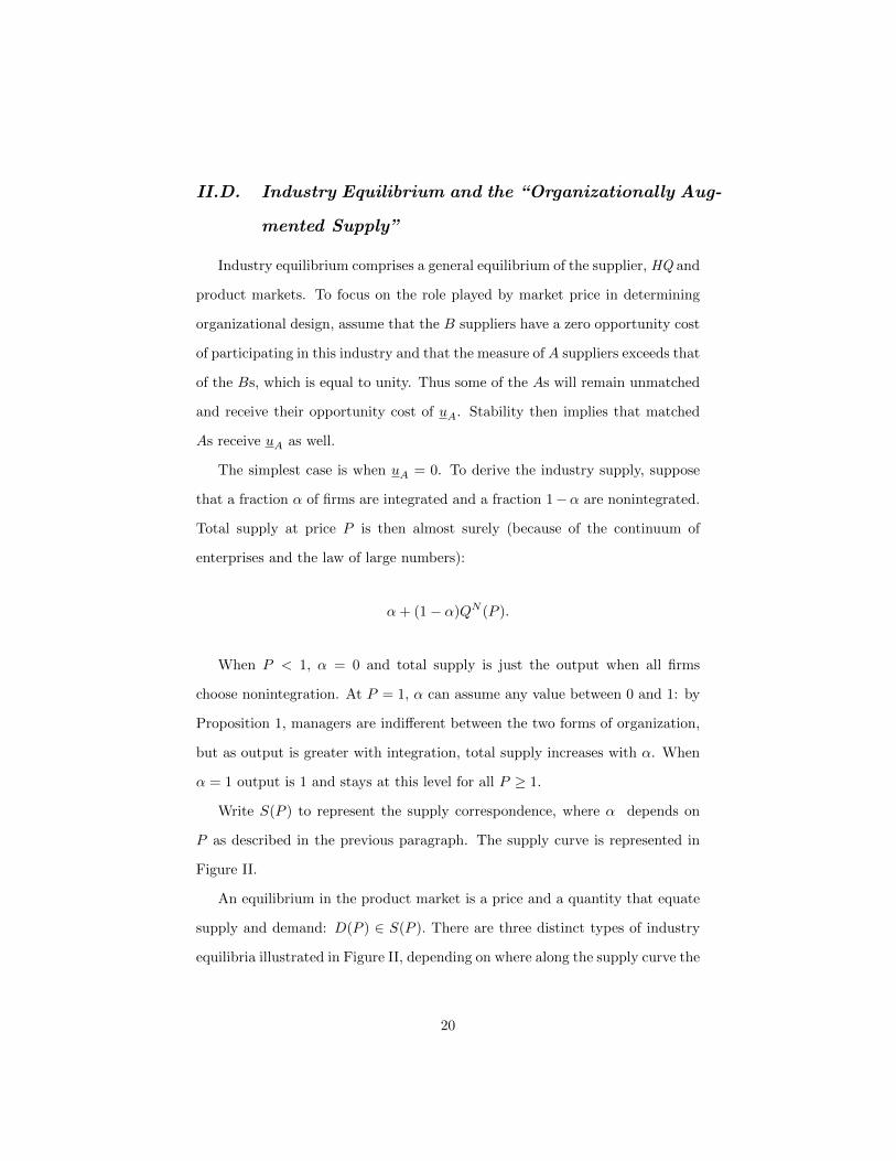
II.D. Industry Equilibrium and the “Organizationally Aug-

mented Supply”

Industry equilibrium comprises a general equilibrium of the supplier, HQ and

product markets. To focus on the role played by market price in determining

organizational design, assume that the B suppliers have a zero opportunity cost

of participating in this industry and that the measure of A suppliers exceeds that

of the Bs, which is equal to unity. Thus some of the As will remain unmatched

and receive their opportunity cost of uA. Stability then implies that matched

As receive uA as well.

The simplest case is when uA = 0. To derive the industry supply, suppose

that a fraction α of firms are integrated and a fraction 1−α are nonintegrated.

Total supply at price P is then almost surely (because of the continuum of

enterprises and the law of large numbers):

α+ (1− α)QN (P ).

When P < 1, α = 0 and total supply is just the output when all firms

choose nonintegration. At P = 1, α can assume any value between 0 and 1: by

Proposition 1, managers are indifferent between the two forms of organization,

but as output is greater with integration, total supply increases with α. When

α = 1 output is 1 and stays at this level for all P ≥ 1.

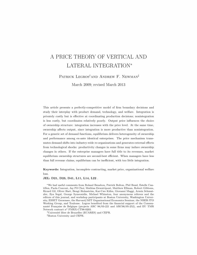
Write S(P ) to represent the supply correspondence, where α depends on

P as described in the previous paragraph. The supply curve is represented in

Figure II.

An equilibrium in the product market is a price and a quantity that equate

supply and demand: D(P ) ∈ S(P ). There are three distinct types of industry

equilibria illustrated in Figure II, depending on where along the supply curve the

20

Q

P

1

N

M

3/4

I

1

Figure II: Organizationally Augmented Supply Curve when uA = 0

equilibrium price occurs: those in which firms integrate (I), the mixed equilibria

in which some firms integrate and others do not (M), and a pure nonintegration

equilibrium (N). The model predicts a monotonic relationship between price

and integration. As demand increases, the equilibrium price increases, inducing

a greater tendency to integrate.

For small positive values of uA (specifically, uA < 1/2) the supply curves

are the same as when uA = 0 except that (i) the shift to integration happens

at a price P ∗(uA) that is greater than 1 and increasing in uA; and (ii) supply is

positive only if P is large enough to generate a surplus of at least uA.16

The airline industry displays a pattern of ownership between major and re-

gional carriers that can be interpreted as movement along the OAS (see Forbes

16. Use the equilibrium condition uA = uA, the indifference locus uA = uB − P1+P

, and A’s

value of integration there uA = P − 12− uB to obtain P ∗(uA) as the solution to

uA = P2

2(1+P )− 1

4. The case uA > 1

2leads to the interesting theoretical possibility of a

nonmonotonic supply curve.

21

and Lederman, 2009; 2010). The good required by a traveller will often con-

sist of two complementary flight segments, one served by the regional carrier

and one served by the major, which corresponds rather closely to the situation

modeled here. Majors own some regional flights (integration) and outsource to

independent firms for others (nonintegration).

The evidence suggests first that integrated relationships perform better (fewer

delays and cancellations), just as in the model, and second, that integration is

more prevalent on routes with high demand or where there are higher costs of

delay (regional routes with endpoints that have more of the major’s departing

flights or that involve a hub). Because P is the revenue lost when a good fails

to be delivered, it is a cost of delay as well as a reflection of demand. Whether

one interprets the involvement of a hub or a high number of connections as

high demand or large delay cost, the model’s basic prediction that integration

is associated with higher enterprise value (P ) is consistent with this evidence.

III. Conduct and Performance of an

Organizational Industry

This section discusses three properties of the model that pertain to industry

conduct and performance. First, there is robust coexistence of different own-

ership structures. Second, the organization of one enterprise depends not only

on its own technology and managers’ preferences but also on prices determined

outside it, implying that “local” changes can have industry-wide effects. Third,

equilibrium has welfare properties readily characterized in terms of consumer

and producer surplus. The model is then used to make sense of evidence from

the ready-mix concrete industry.

22

III.A. Heterogeneity of Ownership Structure

In the mixed region of the OAS (M) there is coexistence of organizational

forms (ownership structure) within the industry. Notice that this organizational

heterogeneity is an endogenous consequence of market clearing given a discrete

set of ownership structures, and occurs even though all firms are ex-ante iden-

tical.

There is much evidence of productivity variation within industries even

among apparently similar enterprises; Syverson (2011) notes that within 4-digit

SIC industries in the U.S. manufacturing sector, a “plant at the 90th percentile

of the productivity distribution makes almost twice as much output with the

same measured inputs as the 10th percentile plant” and that other work on

Chinese or Indian firms find even larger differences. Moreover, as pointed out

by Gibbons (2006, 2010), there is much evidence of correlation between orga-

nizational and productivity variation. The airline case (Forbes and Lederman

2009, 2010) discussed earlier is an example: major airlines own some of their

regional flights (integration) and outsource others (nonintegration), even among

flights with the same origin airport on the same day, and despite the superior

performance of the integrated relationships. But there is little theoretical work

attempting to explain how these organizational and performance differences can

persist.17 The model here provides a simple explanation for part of this cor-

relation, since whenever they coexist, a nonintegrated enterprise generates less

expected output than an integrated one.

Observe that while there is only a single price at which the heterogeneous

outcome occurs, it is generated by a generic set of demand functions:

17. Beside the recent paper by Gibbons, Holden and Powell (2012) discussed in the Intro-duction, there is an early contribution by Hermalin (1994), which obtains heterogeneity inincentive schemes in a principal-agent model when the product market is imperfectly compet-itive.

23

Proposition 2. Consider any demand function D(P ) that is positive and has

finite elasticity at P = P ∗(uA). There exists a nonempty open interval

(δ, δ) ⊂ R+ such that for any demand function δD(P ), with δ ∈ (δ, δ), there

is a mix of nonintegrated and integrated firms in equilibrium.

Recall that the pool of HQs is large enough to integrate every enterprise. If in-

stead the HQs are in short supply, heterogeneity is even more endemic. Indeed,

at all prices exceeding P ∗(uA), managers would prefer integration if the HQs

continued to accrue zero net surplus, but since there are not enough HQs to go

around, some enterprises must be nonintegrated; in equilibrium, HQs extract

enough surplus to render managers indifferent between integration and nonin-

tegration. Similarly, admitting lotteries among ownership structures would also

make heterogeneity easier to obtain.

In contrast to the robust co-existence of ownership structures found here,

other papers investigating endogenous heterogeneity (notably Grossman and

Helpman 2002) have found it to be nongeneric, occurring only for a singular set

of parameters. Further consideration of the difference in results is deferred to

the discussion of entry in Section IV.A.

III.B. Supply Shocks and External Effects

All enterprises face the same price, so anything that affects it – a demand

shift, foreign competition, or a tax on profits – can lead to widespread and si-

multaneous reorganization, as in a merger or divestiture wave. Straightforward

demand and supply analysis can be used to study these phenomena. For in-

stance, growth in demand might raise the price from below P ∗(uA) to above it,

resulting in a merger wave as firms switch from nonintegration to integration.

By the same token, the organization of a particular enterprise depends not

only on its own technology and managers’ preferences but also on prices (prod-

24

uct price and surplus division) determined outside it. In particular, techno-

logical “shocks” that directly affect some firms may induce reorganizations to

other firms that are unaffected by the shock, as well as to themselves; in fact,

sometimes only the unaffected firms reorganize, as in the following example.

A positive technological shock (e.g., a product or process innovation) raises

the success output in joint production to R > 1 for a fraction z of the B-

suppliers. For these affected enterprises, expected output is now equal to

QN (RP )R under nonintegration and to R under integration. Assuming that

uA = 0, so that P ∗(uA) = 1 (positive uA is similar), managers are indifferent

between the two ownership structures when PR = 1: integration occurs for

the innovating firms if the new equilibrium price is greater than 1/R. For the

unaffected firms, the supply correspondence is unchanged. The industry supply

is a convex combination of the supplies for the affected and unaffected firms. In

particular, the supply is increasing in z.

Let demand have constant elasticity, D(P ) = P−ε, with ε > 1. In the

absence of a shock (z = 0), the market clearing condition S(P ) = D(P ) requires

that P = 1; in this case S(1) = D(1) = 1 and though managers are indifferent

between the two ownership structures, market clearing requires that all firms

are integrated.

Consider two cases.

Homogeneous shocks: z = 1. All firms success output is now R∗ > 1. If

all firms are integrated, which requires that in the new equilibrium, P ∗ > 1/R∗,

the market clearing condition is R∗ = (P ∗)−ε, or P ∗ = 1/R∗(1/ε) > 1/R∗,

where the inequality follows from the fact that R∗ and ε both exceed 1. If

a positive measure of firms were nonintegrated, then P ∗ ≤ 1/R∗, but then

demand (P ∗)−ε ≥ (R∗)ε> R∗ would exceed supply. Thus, the only equilibrium

has no change in organization after the shock – all firms remain integrated, and

25

industry output increases to R∗.

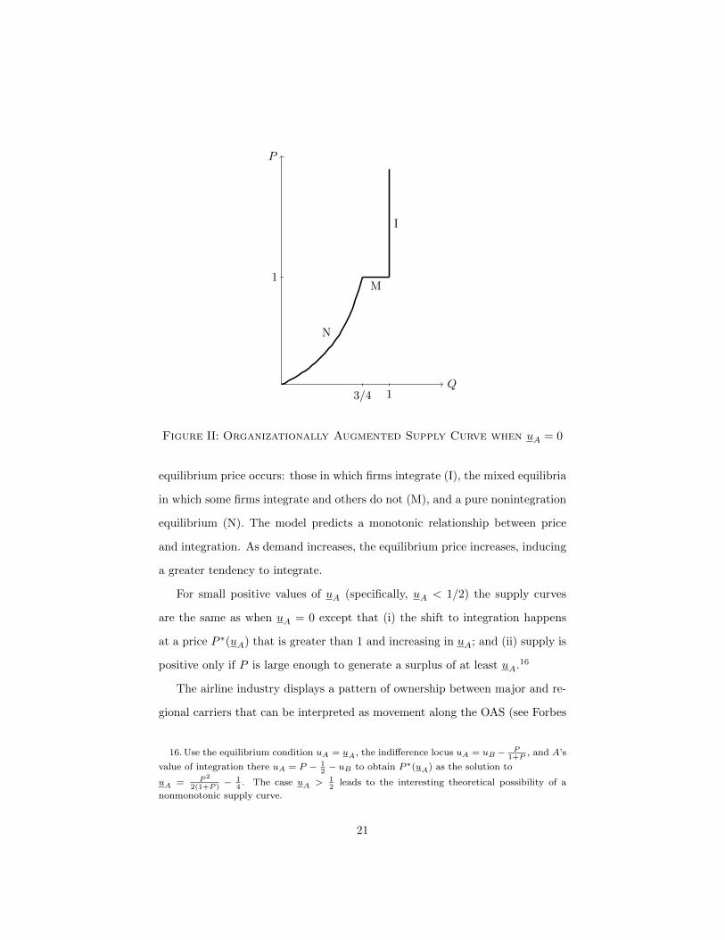
Heterogeneous shocks: z < 1. Suppose the affected enterprises are sub-

ject to a larger shock R > R∗, where the average productivity change is the

same, that is:

zR+ 1− z = R∗.

Since supply is increasing in z, the new equilibrium price cannot exceed 1.

On the other hand, since supply is bounded above by R∗, from the calcula-

tion done above for homogeneous shocks, equilibrium price will always exceed

1/R∗ > 1/R, so none of the shocked firms re-organize. In fact, market clearing

will require that at least some of the unshocked firms reorganize by becoming

nonintegrated: if the price falls below 1, all of them do, and if it remains at 1,

they cannot all remain integrated, for supply would be R∗, exceeding demand,

which is 1. This is an example of an organizational external effect : the impetus

for organizational change may come from outside the firm, transmitted by the

market.

Because the newly nonintegrated enterprises produce less then they did

before, there is a “reorganizational dampening” effect from the heterogenous

shocks: in contrast to the homogeneous case, aggregate output must end up

being less than R∗. In fact, in case the price remains at 1, which obtains for

an open set of parameter values, all of the productivity increase is absorbed

by reorganization; some managers (the innovating Bs) benefit, but consumers

do not.18 It would be difficult to get this kind of effect in a competitive model

with neoclassical firms: two distributions of shocks that lead to the same aggre-

gate production set, as in this case, would lead to the same output and price

outcome.

18. For the price to remain at 1 requires that demand exceed supply when all unshockedenterprises are nonintegrated, or zR+ (1− z)QN (1) ≤ D(1) = 1; using the defining equationfor R and QN (1) = 3

4, this is equivalent to z + 4R∗ < 5.

26

This example may be summarized by saying:

• A firm benefiting from a significant change in technology need not re-

organize.

• A firm that undergoes a large re-organization need not have experienced

any change in technology.

• Re-organizational dampening may substantially absorb the aggregate ben-

efit of heterogenous technological improvements.

Much empirical work in the property rights or transaction cost tradition on

the determinants of integration has focused on “ supply-side” factors, e.g., asset

specificities or complementarities (see, e.g., Whinston 2001 for a summary). The

present model points to the importance of demand: once taken into account,

the simple intuition of supply-side analysis may be overturned.

III.C. Welfare

Since integration is the more productive ownership structure, consumers

benefit when more firms integrate. A natural question to ask is whether there

are equilibria that suffer from “too little” integration. If one follows the indus-

trial organization convention and focuses on total welfare of all the industry’s

participants, then the benefits that consumers experience from more integra-

tion must outweigh any losses in terms of private costs that others (particularly

managers) might suffer.

Consider a central planner who imposes an ownership structure on each

enterprise, but allows participation, noncontractible decisions, prices and quan-

tities to be determined by the market. Define an equilibrium to be ownership

efficient if welfare cannot be increased by imposing on some enterprises an

ownership structure that differs from the one they choose in equilibrium. Since

27

such forced re-organization may hurt the B managers (A managers always get

their opportunity cost), if the planner can make lump sum transfers from the

beneficiaries of the reorganization to the managers, then ownership inefficient

equilibria are also Pareto inefficient. Notice this criterion is weak in the sense

that it does not empower the planner to set the managerial shares s, let alone

the decisions a and b, for any enterprise.19 In what follows, confine attention to

the most straightforward case, where uA <12 .

1. Full Revenue Claims

The analysis of ownership efficiency follows the familiar competitive logic.

Let π denote the success revenue of the managers. Since every A manager gets

his opportunity cost regardless of the ownership decision, a marginal B manager

effectively decides to integrate if the revenue from the extra expected output

generated by integration, valued at π per unit, exceeds his private cost. If in

turn π is also the value to consumers of that extra output, then their willingness

to pay equals the cost, and the outcome is efficient. In equilibrium, consumers

value the extra output at the price P . Thus, π ≡ P implies:

Proposition 3. When managers have full residual claim on revenues, equilib-

ria are ownership efficient.

2. Managerial Firms

One thing that distinguishes the welfare analysis of an organizational indus-

try from the standard competitive one is that often the architects of ownership

19. A stronger concept of efficiency would also allow the planner to impose the share s.In this case, it is welfare maximizing to set s = 1/2 whenever there is nonintegration, whichwould never be part of an equilibrium when the opportunity cost uA is low and managershave no initial wealth. However, this higher welfare would be generated at the expense ofthe B-managers in favor of the As, who would not be able to make lump-sum compensatingtransfers. Indeed, as is shown in Section IV.C, if the As had the cash to make such transfers,they would choose s = 1/2 themselves.

28

structure do not have a full pecuniary stake in the enterprise. If the managers

claim only a fraction of the revenue per unit of output (π < P ), with the re-

mainder accruing to “shareholders,” then they will tend to underweight output,

relative to its social value, in favor of their private costs. Production and orga-

nization decisions are governed by the managers’ unit return π rather than the

market price P , and the industry supply curve will be shifted to the left: output

under nonintegration will be smaller at each price than in the case of full residual

claims (integration output will continue to be equal to 1). More interestingly,

the market price at which firms integrate will increase, since managers will be

content to integrate only when π ≥ P ∗(uA). The fact that marginal output

has a social value of P means that in the managerial firm case, the choice of

organization need not maximize social welfare: there is now a possibility of too

little integration.

To pursue this point, consider the simplest possible representation of di-

luted pecuniary stakes, in which shareholders are “passive” and receive a price-

independent dividend of 1− γ per unit of revenue. The shareholders, like HQs,

only care about income. However they are unable to choose either the revenue

share accruing to the managers or the contractual variables (ownership struc-

ture and s), decisions over which remain with the managers.20 Similarly, the

planner is not empowered to alter γ.

For managerial enterprises, ownership inefficiency is quite common:

Proposition 4. Suppose that managers pay a proportion 1− γ of the revenue

as dividends to shareholders (γ < 1). There is a generic set of demand

20. Section IV.D provides a summary discussion of how the presence of active shareholders,who choose only their dividend share 1 − γ optimally, potentially as a function of the pricelevel, has little impact on the results, whereas if they choose ownership structure as well,they are apt to integrate too often. As long as the managers cannot “buy the firm” from theshareholders by using cash (borrowing for this purpose will not help since the debt repaymentis akin to having γ < 1 from the managers’ perspective), any second-best contract betweenshareholders and managers will entail a residual share γ < 1 for them, leading to ownershipinefficient choices, either by them or by shareholders if the latter are “active”.

29

functions for which equilibrium is ownership inefficient.

To see this, suppose the equilibrium price is P , with the fraction α of integrated

enterprises less than one; thus D(P ) < 1 and P ≤ P ∗(uA)/γ. Each noninte-

grated enterprise bears managerial cost φ(γP ), while integrated ones bear cost

12 .21 Suppose the planner forces a single enterprise to increase its output via a

small increase in (the probability of) integration dα (there is no effect on the

market price). This raises its output by (1 − QN (γP ))dα and the enterprise’s

managerial cost by ( 12 − φ(γP ))dα. Thus the marginal cost of this output in-

crease is12−φ(γP )

1−QN (γP ). If this is less than the consumers’ marginal willingness

to pay, which is equal to the equilibrium price P , then the planner’s forced

integration has increased welfare, and equilibrium is ownership inefficient.

It is not hard to find prices at which this can happen: simply let P =

P ∗(uA))/γ, the market price at which managers are indifferent between the two

ownership structures. Then the planner’s marginal cost is12−φ(P

∗(uA))

1−QN (P∗(uA)), which by definition is equal to P ∗(uA). Since γ < 1, P > P ∗(uA),

i.e., it exceeds the planner’s marginal cost, and there is ownership inefficiency.

Notice that this equilibrium price also generates coexistence of the two owner-

ship structures. Thus, with managerial firms, heterogeneity implies inefficiency.

From Proposition 2, the set of demands that generate coexistence, and therefore

ownership inefficiency, is generic.

Typically, though, inefficiency is more endemic than heterogeneity.22 Mak-

ing γ small ensures a wide range of inefficient equilibrium prices, including some

21. Denote by φ(π) the total private cost for a pair of managers under nonintegration whentheir revenue is π, which is (s2+(1−s)2)(π)2(1+π)−2, where s satisfies sπQN (π)−s2(π)2(1+π)−2 = uA. The notation suppresses the dependence of φ(·) on uA.

22. Since the inverse demand and the planner’s marginal cost are continuous in P , thestrict inequality between them that holds at P ∗(uA)/γ also holds on an open interval ofprices below that, so there is inefficiency there. Moreover, since s2 + (1− s)2 ≥ 1

2, φ(γP )) ≥

12

(γP )2(1+γP )−2, and the planner’s marginal cost is bounded by 12

+γP . Thus, for ownership

inefficiency it suffices that P lie betweenP∗(uA)

γand 1

2(1−γ) , a range that is nonempty if

γ < 2/3, since P ∗(uA) ≥ 1.

30

below P ∗(uA) (γ need only be less than 1/2). The reason forced integration is

beneficial at such low prices is that nonintegration is especially poor at output

production when managers are not full revenue claimants — a kind of “inten-

sive margin” inefficiency, which supplements the “extensive margin” inefficiency

wherein they only integrate at excessively high prices.

All of this says little about the size of the welfare loss, or precisely the

extent to which the planner should integrate to maximize welfare. For more

than marginal amounts of forced integration, there will be a decrease in the

market price: this reduces the welfare gains from such policy, both because of

the reduction in willingness to pay and (at least when uB > uA) reduced costs of

nonintegration. Thus, demand elasticity plays a role in determining the extent

of inefficiency, just as it does in market power settings, but as is shown next, its

effect is quite different.

3. Graphical Analysis and the Role of Demand Elasticity

A simple illustration of Propositions 3 and 4 can be obtained when uA = 0.

In this case, under nonintegration s ≡ 0 and A therefore chooses a = 1 regardless

of the output price. B’s choice of b therefore determines expected output. Since

s ≡ 0, φ(π) = π2(1 + π)−2. It is helpful to write this in terms of quantity q

using the invertibility of QN (·): if q = QN (π), φ(π) = c(q) ≡ (1−√

1− q)2.

Suppose the enterprise produces expected output Q ≤ 1 by randomizing

between integration with output 1, and nonintegration with expected output q.

Then the integration probability α must be Q−q1−q , and the cost of this production

strategy is α 12 +(1−α)c(q). Let C(Q) ≡ minq≤Q α 1

2 +(1−α)c(q) (the constraint

q ≤ Q derives from the requirement α ≥ 0). The solution is the interior optimum

34 if Q > 3

4 ; else the constraint binds and the optimum is q = Q. Thus the

marginal cost is C ′(Q) = c′(Q) for Q < 34 and C ′(Q) = 1 for Q > 3

4 .

Maximizing B’s payoff πQ − C(Q) subject to A receiving his opportunity

31

cost of 0 implies that the equilibrium level of output solves π = C ′(Q). If γ =

1, π = P (full revenue claims), yielding the conventional efficient equilibrium

characterization that price equals marginal cost, as in Proposition 3. In other

words, when uA = 0, the full-revenue-claim supply coincides with the marginal

cost schedule. Efficient production corresponds to the intersection of demand

with this schedule. But for γ < 1, π = γP < P : the marginal cost of production

is lower than the price (when the price is less than 1/γ), and there is too little

production, both because nonintegration produces less than it should (intensive

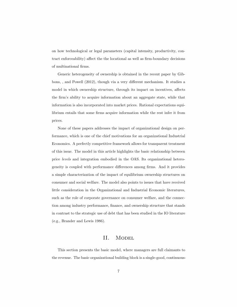
margin) and because there is too little integration (extensive margin).

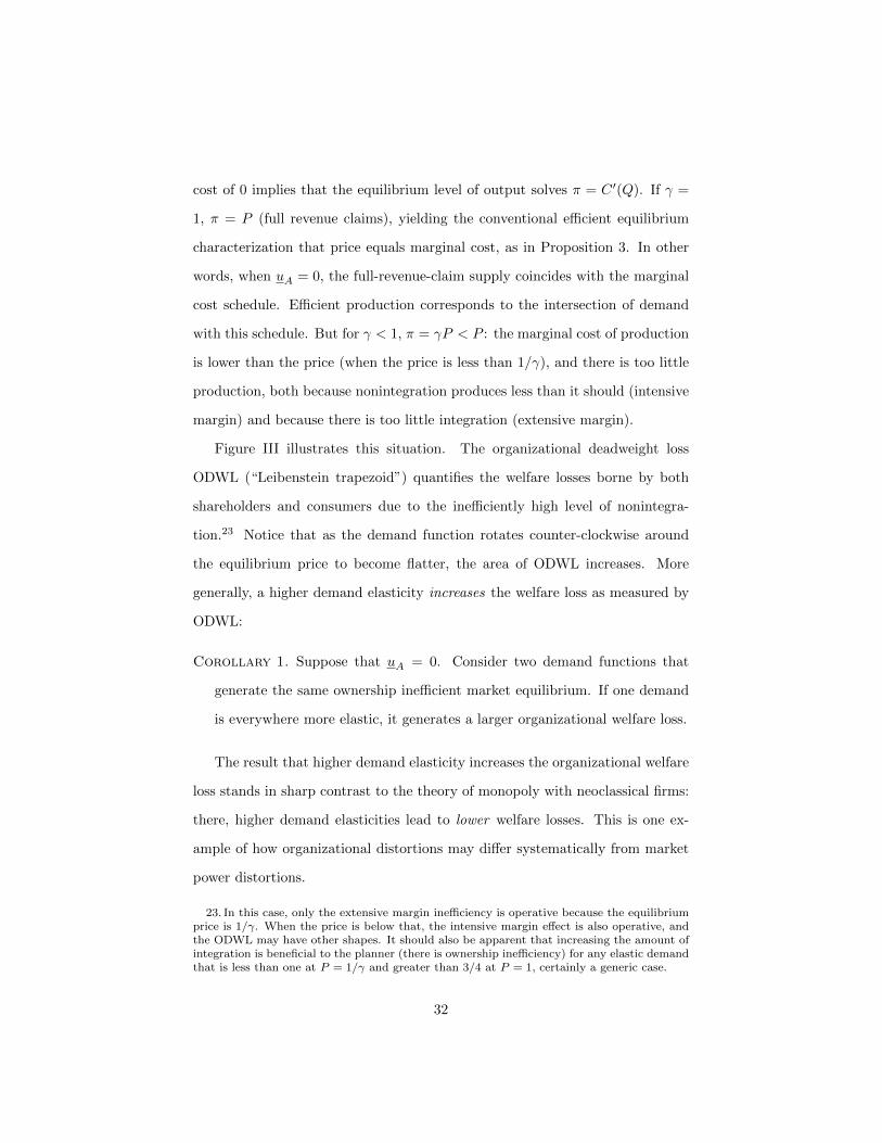
Figure III illustrates this situation. The organizational deadweight loss

ODWL (“Leibenstein trapezoid”) quantifies the welfare losses borne by both

shareholders and consumers due to the inefficiently high level of nonintegra-

tion.23 Notice that as the demand function rotates counter-clockwise around

the equilibrium price to become flatter, the area of ODWL increases. More

generally, a higher demand elasticity increases the welfare loss as measured by

ODWL:

Corollary 1. Suppose that uA = 0. Consider two demand functions that

generate the same ownership inefficient market equilibrium. If one demand

is everywhere more elastic, it generates a larger organizational welfare loss.

The result that higher demand elasticity increases the organizational welfare

loss stands in sharp contrast to the theory of monopoly with neoclassical firms:

there, higher demand elasticities lead to lower welfare losses. This is one ex-

ample of how organizational distortions may differ systematically from market

power distortions.

23. In this case, only the extensive margin inefficiency is operative because the equilibriumprice is 1/γ. When the price is below that, the intensive margin effect is also operative, andthe ODWL may have other shapes. It should also be apparent that increasing the amount ofintegration is beneficial to the planner (there is ownership inefficiency) for any elastic demandthat is less than one at P = 1/γ and greater than 3/4 at P = 1, certainly a generic case.

32

0Q

P

QN (γP )

Supply(γ < 1)

1/γ

1

d

d

C ′(Q)

ODWL

3/4 1

Figure III: Ownership Inefficiency when γ < 1 and uA = 0

III.D. An Empirical Illustration: Cement and Concrete

Hortacsu and Syverson (2007) studies the vertical integration levels and

productivity of U.S. cement and ready-mixed concrete producers over several

decades and many local markets. They find that these industries are fairly com-

petitive, that demand is relatively inelastic, and that there is little evidence that

vertical-foreclosure effects of integration are quantitatively important. Three of

their major findings are (a) prices are lower and quantities are higher in markets

with more integrated firms, (b) high productivity producers are more likely to be

integrated, and (c) some of the more productive firms are nonintegrated. They

tie the productivity advantages to improved logistics coordination afforded by

large local concrete operations, regardless of whether it presides in integrated

or nonintegrated enterprises.

Though the negative correlation between integration and prices would go

against a single-productivity version of the model, shutting down productivity

variation is obviously a simplification imposed to highlight the importance of

33

demand in determining ownership structure. The importance of supply-side

factors (relationship specificity, complementarity of assets and investments, and

the like) has received the bulk of the emphasis in the literature.

As shown in Section IV.B, higher productivity implies integration will occur

at lower prices, so the Hortacsu-Syverson findings (a) and (b) are explained by

the presence, which is documented in the paper, of multiple productivity levels,

interpreted as exogenous — markets with more integrated firms are likely to be

those with more productive firms, so equilibrium prices will be lower, assuming

equal demands.

However, technological variability by itself (and models which exploit this

as their only source of variation in organizational form) cannot fully explain

the findings either: if higher productivity causes integration, why aren’t all

productive firms integrated, in contradiction to finding (c)? Neither supply

alone, nor demand alone would seem to be able to explain the facts of the U.S.

concrete and cement industries. But together they can.

Suppose, as in Section III.B, that there is exogenous variation in the pro-

ductivity of the enterprises in the industry, specifically two productivity levels,

1 and R, with 1 < R. Demand is isoelastic, with D(P ) = 34P−1, and uA = 0.

Letting z be the proportion of high productivity firms, the equilibrium price at

z = 0 is P = 1 and all (low productivity) firms are nonintegrated. As z increases

in the interval (0, 1) the equilibrium price will decrease from 1 to 1/R.

If the price is strictly larger than 1/R, low productivity firms choose non-

integration while high productivity firms choose integration. If price is equal

to 1/R, some of the high productivity firms will be nonintegrated. Either way,

high productivity firms are more likely to be integrated, as in finding (b).

As long as P > 1/R, the proportion of integrated firms is z, and the equi-

34

librium price solves:

zR+ (1− z)QN (P ) =3

4P−1,

where the left hand side is the industry supply given the organizational choices

of high and low productivity firms, and the right hand side is the demand. As

z increases, the equilibrium price decreases. Thus, consistent with finding (a),

price is negatively correlated with the degree of industry integration.

For z above z∗, where z∗R+ (1− z∗)QN (1/R) = 34R, the equilibrium price

is 1/R. At this price managers in high productivity enterprises are indifferent

between integration and nonintegration. Some high productivity firms will have

to be nonintegrated in order to satisfy the market clearing condition, whereas

the low-productivity firms continue to be nonintegrated. Hence, there will be

heterogeneity of ownership structure among high productivity enterprises, as in

finding (c). Of course, this computation assumes the coexistence of integrated

and nonintegrated plants is within a local market. For coexistence across mar-

kets, it is enough to posit that they have different demands. Either way, the

evidence on cement and ready-mix concrete highlights the importance of de-

mand as well as supply for understanding the determinants of ownership and

its relation to industry performance.

IV. Extensions

This section sketches some extensions of the basic model and some directions

for future research.

35

IV.A. Entry

The model considered so far has a fixed population of price-taking suppliers,

corresponding to the standard Arrow-Debreu notion of competition. Industrial

Economics is also concerned with ease of entry, which in the present model

would also include the choice of “side” (A or B). Since managers (particularly

Bs) earn rents, it is fair to ask what happens if these rents could be competed

away.

Consider the following simple model of entry. There is an unlimited popula-

tion of ex-ante identical potential entrants, each of whom receives zero outside

the industry and can choose to become an A or a B. If nA and nB are the

measures of people choosing A and B respectively, the cost of entry borne by

an individual entrant is eA(nA) = e(nA), eB(nB) = βe(nB) where e(·) is a non-

decreasing function: one side takes a larger investment than the other, unless

β = 1, and resources devoted to training for either side become scarce as the

industry expands.24

A (long-run) equilibrium will consist of measures nA and nB of entrants

on each side; a market clearing product price P and quantity D(P ); and fea-

sible payoffs uA and uB for each of the entrants, according to which side they

take. In equilibrium agents are indifferent among the two occupations and re-

maining outside the industry, and markets clear; this requires in particular that

nA = nB . The scale (measure of A-B pairs) of the industry will be the com-

mon value n. In the product market, supply embodies ownership choice, as

before; following Proposition 1 the ownership decisions, and therefore industry

output, are determined jointly by |uA − uB | and P. The supply of the industry

24. The baseline model is equivalent to having a fixed set of B suppliers, while entry or exitinto A or HQ supply is permitted; then uA = e(1), while as before the opportunity cost ofHQs is zero. The long run analysis also allows entry into B supply. This abstracts from issuessurrounding the financing of entry, which in light of the discussion in Section IV.C below,alters little.

36

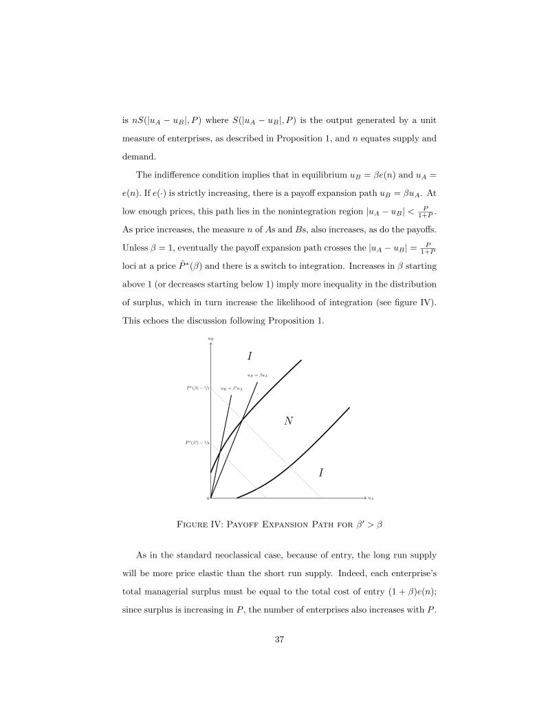
is nS(|uA − uB |, P ) where S(|uA − uB |, P ) is the output generated by a unit

measure of enterprises, as described in Proposition 1, and n equates supply and

demand.

The indifference condition implies that in equilibrium uB = βe(n) and uA =

e(n). If e(·) is strictly increasing, there is a payoff expansion path uB = βuA. At

low enough prices, this path lies in the nonintegration region |uA − uB | < P1+P .

As price increases, the measure n of As and Bs, also increases, as do the payoffs.

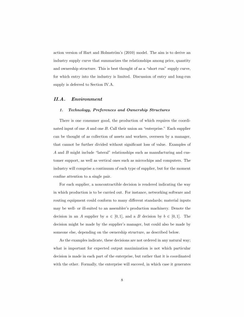
Unless β = 1, eventually the payoff expansion path crosses the |uA − uB | = P1+P

loci at a price P ∗(β) and there is a switch to integration. Increases in β starting

above 1 (or decreases starting below 1) imply more inequality in the distribution

of surplus, which in turn increase the likelihood of integration (see figure IV).

This echoes the discussion following Proposition 1.

0

uB

uA

N

I

I

uB = βuA

uB = β′uAP ∗(β)− 1/2

P ∗(β′)− 1/2

Figure IV: Payoff Expansion Path for β′ > β

As in the standard neoclassical case, because of entry, the long run supply

will be more price elastic than the short run supply. Indeed, each enterprise’s

total managerial surplus must be equal to the total cost of entry (1 + β)e(n);

since surplus is increasing in P , the number of enterprises also increases with P .

37

Thus the price response of each enterprise is augmented by an increase in their

number, leading to a more elastic supply than in the short run (in particular,

the integration portion of the long run supply is no longer vertical).

Where managers are indifferent between integration and nonintegration, the

quantity supplied will depend on the fraction of integrated enterprises, but their

number is fixed. Thus, as in the short run, the supply curve has a horizontal

segment at P ∗(β), and there is generic heterogeneity of organizational forms in

a free-entry equilibrium.

In the special case where e(n) is a constant, the payoff expansion path is de-

generate; the payoffs uA, uB are independent of demand. For almost all values

of the cost of entry, the vector of equilibrium payoffs will lie either in the non-

integration or integration region, making heterogeneity of organizational forms

a nongeneric outcome. This is similar to the Grossman and Helpman (2002)

finding.

Finally, the short run welfare results extend to the long run; the equilibrium

will be ownership efficient if γ = 1 but not in general otherwise.

IV.B. Scale and Scope

So far, enterprises produce at most one unit of output, but it is not difficult

to extend the model to allow for variation in enterprise scale, employee quality

or other contractible input level. Suppose that enterprises may increase the

volume of successful production by a multiplicative factor f(l), a function of

some contractible input l that represents quantity or quality, at cost represented

by the schedule w(l). Then expected profit is (1 − (a − b)2)f(l)P − w(l). For

simplicity assume that the private managerial cost is unaffected by l. The

input is paid contingently on success: the amount paid, d(l), satisfies (1− (a−

b)2)d(l) = w(l), with a, b assuming their equilibrium values (equivalently, a loan

38

can be procured ex-ante to pay the input and the loan is repaid upon success).

When enterprises form, managers contract on shares, ownership structure, and

scale; then noncontractible decisions a, b are chosen last.

As before, the success probability under integration will be 1; assuming

differentiability of f(·) and w(·), the integration scale lI will satisfy:

Pf ′(lI) = w′(lI).

For the nonintegrated enterprise, a straightforward computation shows that its

scale lN satisfies:

QPf ′(lN ) = w′(lN ),

where Q = QN (Pf(lN )− d(lN )). Thus marginal returns to l are greater under

integration. From Topkis’s theorem, lI > lN . And as before, there will be a

price at which managers are indifferent between integration and nonintegration.

Hence, when they coexist, integrated firms are bigger or “smarter” (in the

alternative interpretation of l as quality) than nonintegrated ones.25 Therefore

the output gap between the two kinds of enterprises is amplified. Whether these

endogenous output differences could explain the large productivity differences

that observed in many industries is left for further research. Some indication of

its plausibility is offered by Hortacsu and Syverson (2007), which reports that

integrated cement and concrete producers are larger and more capital intensive,

as well as more productive, than nonintegrated ones.

Another extension of the model involves the analysis of firm scope, wherein

each supplier produces its own distinct good for sale on the market, as in

the original Hart-Holmstrom model. Because it involves strategic interactions

25. This result persists if l represents a vector of complementary inputs, or if managerialcosts are a function of the scale, as long as these costs do not grow too quickly with respectto l. Details available upon request.

39

among different parts of the enterprise, this case is somewhat intricate, particu-

larly if the number of suppliers is greater than two. Legros and Newman (2010)

considers such a model. As here, integration yields coordination but at a high

cost for the managers of individual product lines. Moreover, an integrated firm

provides coordination benefits not only to its members, but also for “outsiders,”

who can free ride. The integrated firm is typically tempted to follow the pref-

erences of the outsiders, who therefore enjoy coordination benefits at lower cost

than insiders. This mechanism provides a limit to the extent of integration,

and the paper shows that the scope of multi-product firms depends on both the

mean and the variance of individual product prices.

IV.C. Finance

The responsiveness of ownership choice to industrial conditions in the model

emerges in large measure because managers have finite (in fact, zero) wealth.

This assumption implies that the ownership structure is dependent on the dis-

tribution of surplus between them, and that in turn leads to the relationship

between industry price and degree of integration embedded in the OAS. It is

worth devoting some attention to the comparative statics of the wealth endow-

ments, as this appears to be connected more generally to the role that financial

contracting would have in affecting industry performance.

One important difference between integration and nonintegration is the de-

gree of transferability in managerial surplus: while managerial welfare can be

transferred 1 to 1 with integration (that is one more unit of surplus given to B

costs one unit of surplus to A) by adjusting the revenue shares, this is not true of

nonintegration. If the A manager has cash that can be transferred without loss

to the B manager before production takes place, the advantage of integration

in terms of transferability is reduced. This has immediate consequences for the

40

OAS.

Proposition 5. Positive increases in the cash endowments of A suppliers shift

the OAS to the left and decrease the level of integration.

In particular, if managers have access to infinite amounts of cash, they will

always contract for equal sharing in nonintegrated organizations. However, for

any finite cash holdings, there is a level of price high enough for which there

will be integration.

These observations apply with equal force when the managers are not full

residual claimants on the revenues of the firm. Since integration is output

maximizing, giving managers cash increases the inefficiencies from the point of

view of consumers and shareholders. Thus, in contrast to previous literature

that has suggested that managerial cash holdings may lead to firms that are too

large, this model suggests it may generate firms that are too small.26

Borrowing can sometimes be a substitute for cash, but its efficacy depends

on the ownership structure. In general, if the income stream one is borrowing

against is subject to incentive problems, then borrowing is a poor substitute;

if not then it is at best equivalent. Thus, under integration, a cash-poor HQ

can finance the acquisition with debt without affecting output, and in fact may

borrow essentially up to the value of the enterprise P , provided she puts up at

least some cash. The managers could also use debt for side payments, though

nothing is gained (or lost) by this: re-dividing the asset purchases or the revenue

would accomplish the same thing (recall the integration Pareto frontier is the

off diagonal).

By contrast, under nonintegration, borrowing for side payments is more

limited. If a debt D has to be repaid when the output is high, it is as if the

26. As in Jensen (1986) managers will tend to use cash for their own interest rather thanthat of shareholders or consumers, but while in the free cash flow theory they will tend to usecash for “empire building” or over-expansion, here they use cash to keep firms small and buya “quiet life”.

41

managers face a success revenue of P−D, and expected output will decrease from

QN (P ) to QN (P−D); this leads to a decline in ex-post total managerial welfare

that has to be weighed against the ex-ante lump-sum payment. In the appendix

it is shown that there is no gain to using such contracts when the managerial

surplus allocation is either very unequal (along the axes) or approximately equal

(in a neighborhood of the 45-line). Thus the debt-enhanced nonintegration

frontier “adheres” to the no-debt frontier in those regions; in particular, debt for

side payments does not approximate cash transfers (for instance, cash is Pareto

improving near the 45-line, significantly so near the axes). In between the axes

and the 45-line, small amounts of debt for side-payments may raise managerial

welfare, enlarging slightly the set of prices for which nonintegration is chosen.

Qualitatively, the responses of the integration decision to prices and surplus

division go much as before, but the possibility of borrowing for side payments

not only may reduce the output performance of nonintegrated enterprises, but

also may increase their number. If the managers are not full revenue claimants,

debt may therefore lower total welfare.

Proposition 6. Integrated firms (HQ) may use debt to finance the purchase of

assets. nonintegrated enterprises do not use debt for ex-ante side-payments

if As receive either zero surplus or share surplus equally with Bs.

Note that debt is used here only to finance ex-ante side payments and not

acquisition of assets from outside the relationship. If firms have investment

opportunities, e.g., to expand their scale of production, nonintegrated firms are

at a disadvantage for borrowing since debt has a depressing effect on expected

output.

42

IV.D. Active Shareholders

The model assumes managers have control over the integration decisions

and ownership inefficiencies take the form of too little integration. Since share-

holders have similar objectives to consumers — as price takers, they value high

output — a reasonable conjecture is that efficiency may be improved when

shareholders have control over integration decisions and compensation to man-

agers. Corporate governance is now relevant not only for shareholders but also

for consumers.

Providing good incentives is costly to shareholders under nonintegration,

since it entails giving up a share of profit to management. Hence, if shareholders

have control over the share of revenue accruing to managers, nonintegration will

underperform relative to how it does when managers retain all the revenue. By

contrast, integration performs well at all managerial shares. Shareholders will

therefore tend to integrate “too often.” Thus, while shareholder control may

implement a planner’s forced integration as a means of protecting consumers,

it can be taken too far.

Proposition 7. Suppose that the shareholders control the decision to integrate

and the shares of output going to the two managers. The minimum price at

which shareholders choose integration is strictly lower than the ownership

efficient level.

The policy question of how to regulate governance when consumers are af-

fected by firm’s organizational choices is still open and an important subject for

future research.

43

V. Conclusion

By embedding a simple model of the determination of firm boundaries into

a perfectly competitive setting, this paper suggests that internal organizational

effects can have significant consequences at the industry level, quite apart from

the strategic and collusive interactions among firms that have dominated the

Industrial Economics literature. The model’s organizational industry equilib-

rium offers an explanation for heterogeneity in firm performance and shows that

the response of the industry to demand or technology shocks is dependent on

integration decisions. At the same time, it illustrates how market forces can be

important determinants of organizational design.

This model of industry equilibrium is based on one important tradeoff be-

tween nonintegration and integration: nonintegration is strong on internalizing

private costs and weak on coordinating decisions; integration has the opposite

strength and weakness. And though there is evidence of the model’s relevance

for the cement and airlines industries, an organizational Industrial Economics

is hardly restricted to this tradeoff. Other underlying models of integration or

other aspects of organizational design may generate other relationships among

prices, quantities and organization: the OAS may have different shapes for

different theories. One benefit of unifying Organizational and Industrial Eco-

nomics is that market data become a proving ground for different organizational

tradeoffs, which can help to identify the relative importance of each in different

contexts.

Although the model goes some way toward the objective of jointly deter-

mining market structure, ownership structure, and industry conduct and per-

formance, much remains to be done. In particular, rather than assuming perfect

competition, environments where market power would play a role could also be

considered, so that the degree of competition would be endogenous.

44

Finally, on the welfare side, the analysis also shows that consumers have

an interest in the organization of the firms that make the products they buy.

An influential strand of thought asserts that competition in the product market

must assure efficient outcomes: firms that do not deliver the goods at the lowest

feasible cost, whatever the reason, including inefficient organization, will be

supplanted by ones that do.27 The present framework confronts such claims

directly. While efficient ownership may prevail when managers have full title

to enterprise revenue, in the general case, organizational choices may not be

efficient. Much as Leibenstein argued, and as quantified by the eponymous

trapezoid, the welfare losses from this kind of organizational inefficiency may

be significant.

Appendix: Proofs

A. Proof of Proposition 3

Suppose that demand is perfectly elastic. With integration, B gets P − 12 −

uA, while with nonintegration he gets uNB (s(P ;uA), P ) = UN (s(P ;uA), P )−uA,

where s(P ;uA) is the sharing rule solving uNA (s, P ) = uA, with uNA (s, P ) defined

in (3).

It follows that the B manager chooses the organization that maximizes the

total managerial welfare. Since with perfectly elastic demand, the total welfare

coincides with the total managerial welfare, the result follows.

With a less elastic demand, suppose that at the market equilibrium some

firms are not integrated. If any firms are forced to integrate, industry sup-

ply increases and therefore the new equilibrium will be at P ′ < P since de-

mand is decreasing. However, the difference in total welfare between forced

27. The “form of organization that survives... is the one that delivers the product demandedby customers at the lowest price while covering costs.” (Fama and Jensen, 1983).

45

integration at price P ′ and nonintegration at price P is bounded above by

U I(P ) − UN (s(P ;uA), P ), which is negative by the previous argument. Hence

the initial equilibrium is ownership efficient.

Finally, if in equilibrium all firms are integrated, forcing some firms not to

integrate will decrease consumer surplus (since the quantity supplied decreases)

and decrease managerial surplus (since managers prefer integration), so equilib-

rium is efficient in this case as well.

B. Proof of Corollary 1

Consider demand functions DL and DH yielding the same ownership ineffi-

cient equilibrium with price P e and proportion αe ≥ 0 of integrated firms (thus

DH(P e) = DL(P e)), and suppose DH has larger elasticity than DL at all prices.

Let Ωi(P ) be the consumer welfare corresponding to the demand Di, i = H,L.

Fix γ < 1 and write the sums of shareholder and managerial payoffs under

integration and nonintegration respectively as

V I(P ) = P − 1

2

V N (P ) = PQN (γP )− φ(γP ).

A planner can choose to force a proportion α firms to integrate in order to

maximize total welfare when demand is Di:

maxα

Ωi(P ) + αV I(P ) + (1− α)V N (P )

s.t. Di(P ) = α+ (1− α)QN (γP ).

The constraint defines a one-to-one relationship between α and P and ρi(α) is

the price solving the constraint for a given value of α. The problem is then

46

equivalent to choosing α to solve:

maxα

Ωi(ρi(α)) + αV I(ρi(α)) + (1− α)V N (ρi(α)).(6)

Clearly, for any α, ρL(α) < ρH(α) < P e.

Fact (i) If DH has larger elasticity than DL at any price, the two demand curves

intersect only once at P e and DH(P ) > DL(P ) for any P < P e.

(ii) For all P < P e, ΩH(P )− ΩH(P e) > ΩL(P )− ΩL(P e).

(iii) If P ≤ P ′ < P e and DH(P ′) = 1, ΩH(P ′)− ΩH(P e) + P ′ − P > ΩL(P )−

ΩL(P e).

Proof. (i) At P e, since DH(P e) = DL(P e), DH is flatter than DL. If

single crossing fails, there is a price less than P e where the demand curve DH

crosses DL from above, hence DH is steeper than DL at P ′, contradicting the

assumption that DH has larger elasticity than DL at any price. (ii) Now, for

P < P e, DH is above DL, implying that the incremental consumer welfare is

larger for DH than DL, as claimed. (iii) By (ii), ΩH(P ′)−ΩH(P e) > ΩL(P ′)−

ΩL(P e). It is clear that ΩL(P ) − ΩL(P ′) < P ′ − P ; substituting ΩL(P ′) >

ΩL(P )− (P ′ − P ) in the previous inequality yields the result.

Case 1. Suppose first that the solution of (6) is obtained at αL = 1, leading

to an equilibrium price of PL = ρL(1). Then total welfare gain is GL(1) =

ΩL(PL) − ΩL(P e) + V I(PL) − V N (P e). If the planner imposes α = 1 with

demand DH (this may not be optimal), the price will be PH = ρH(1); by the

Fact (i), PH > PL and the gain in welfare is GH(1) = ΩH(PH) − ΩH(P e) +

V I(PH)− αeV I(P e)− (1− αe)V N (P e). Therefore:

GH(1)−GL(1) = [ΩH(PH)− ΩH(P e)]− [ΩL(PL)− ΩL(P e)] + PH − PL

47

which is positive by Fact (iii). Because the maximum welfare loss with DH is

at least GH(1), the result follows. Note that this case does not use the fact that

uA = 0.

Case 2. Suppose now that the solution to (6) is obtained at an interior point

αL ∈ (αe, 1), and let PL = ρL(αL). Then:

(7) V I(PL)− V N (PL) > 0.

To see this, use Ω′L(PL) = −DL(PL) to obtain the variation of the planner’s

objective function with respect to α at the optimum as:

dρL(αL)

dα

dQN (γPL)

dP(1− α)γ

[PL − c′(QN (γPL))

]+ V I(PL)− V N (PL).

Because dρL(αL)dα < 0 and P − c′(QN (γPL)) = (1 − γ)PL > 0 (recall from the

text that the nonintegrated enterprise sets π = c′(q)), αL solves the first order

condition only if V I(PL)− V N (PL) > 0, as claimed.

Case 2a. Suppose there is α ∈ (0, 1) such that DH(PL) = α + (1 −

α)QN (γPL). Then α > αL, since DH(PL) > DL(PL). The total gains in sur-

plus when α firms integrate under demand function DH and αL firms integrate

under demand DL are therefore:

GH(α) = ΩH(PL)− ΩH(P e) + V N (PL) + α[V I(PL)− V N (PL)]

− αeV I(P e)− (1− αe)V N (P e),

GL(αL) = ΩL(PL)− ΩL(P e) + V N (PL) + αL[V I(PL)− V N (PL)]

− αeV I(P e)− (1− αe)V N (P e),

48

implying:

GH(PL)−GL(PL) = ΩH(PL)− ΩH(P e)− [ΩL(PL)− ΩL(P e)]

+ (α− αL)[V I(PL)− V N (PL)]

which is positive by Fact (ii), (7), and α > αL. Because the maximum gain

under DH is greater than GH(PL) while GL(PL) is the maximum gain under

DL, the result follows.

Case 2b. The last possibility is that there does not exist α ∈ (0, 1) such that

DH(PL) = α + (1− α)QN (γPL). Then DH(PL) > 1. Let PH = ρ(1). If under

DH all firms are forced to integrate the total surplus is ΩH(PH) +V I(PH). Be-

cause V I(PL) > V N (PL), V I(PH)− [αLVI(PL)+(1−αL)V N (PL)] > V I(PH)−

V I(PL) = PH − PL. Hence:

GH(PH)−GL(PL) = [ΩH(PH)− ΩH(P e)]− [ΩL(PL)− ΩL(P e)]

+ V I(PH)− αLV I(PL)− (1− αL)V N (PL)

> [ΩH(PH)− ΩH(P e)]− [ΩL(PL)− ΩL(P e)] + PH − PL

> 0.

where the last inequality follows Fact (iii).

C. Proof of Proposition 5

Under nonintegration, cash is a more efficient instrument for surplus allo-

cation than the sharing rule s between managers A and B since a change of s

affects total costs. By contrast, when firms are integrated, a change in s has no

effect on output or costs and therefore shares are as efficient at allocating surplus

as cash. Hence, introducing managerial cash endowments favors nonintegration,

49

and there will be fewer integrated firms.

Return to the baseline environment where the population of Bs is fixed and

let uA = 0. Assume for simplicity that all A managers have the same cash

holding `. A contract now specifies a lump sum transfer t from the A manager

to the B manager together with a share s of output and an organization. Be-

cause the managerial surplus is transferable under integration, cash transfers

are neutral. For nonintegration however, since the total surplus is increasing on

s ∈ [0, 1/2], the ability for the A managers to make cash transfers in exchange

for a greater share of output will increase managerial surplus. Final payoffs are

then uNA (s, P )− t and uNB (s, P ) + t, where uNA , uNB are given by (3).

By competition, the marginal manager A must have zero surplus. For a

given market price P , if ` > UN (1/2, P ), A managers are able to transfer t =

UN (1/2, P )/2 to the B manager at the signing of the contract in exchange for

a share of 1/2 of the output. In this case, the payoff to the B managers is

UN (1/2, P ). If ` < UN (1/2, P ), the A manager uses a transfer t = ` in exchange

for a share s`(P ) of the revenue satisfying:

uNA (s`(P ), P ) = `.

In this case, managers B have, after the transfer of t = `, a payoff of:

uNB (s`(P ), P ) + ` = UN (s`(P ), P ).

Recall that UN (s`(P ), P ) = PQN (P ) − ψ(s`(P ))c(QN (P )) with ψ(s) ≡ s2 +

(1 − s)2. Since ψ(s) is a decreasing function of s ∈ [0, 1/2], and since as `

increases, s`(P ) increases, total managerial welfare increases in `. By contrast,

managerial welfare under integration is U I(P ) = P − 1/2 which is independent

of `. Therefore the shift to integration happens at higher prices.

50

D. Proof of Proposition 6

Debt and nonintegration. Suppose that A makes a side payment T to B that

is financed with a debt. Specifically, an amount D is repaid in case of success,

and by limited liability, there is no repayment in case of failure. Then A’s

revenue share s must satisfy sP ≥ D, and the payoffs to the two managers are

respectively uA = (1−(a−b)2)(sP−D)−(1−a)2 and uB = (1−(a−b)2)(1−s)P−

b2+T . By making the change of variable s = sP−DP−D , the payoffs can be written as

uA = (1−(a−b)2)s(P−D)−(1−a)2 and uB = (1−(a−b)2)(1−s)(P−D)−b2+T .

The game in (a, b) played by the managers is then equivalent to the baseline

model of nonintegration with a price equal to P−D. The probability of success is

QN (P −D) and therefore in equilibrium T = QN (P −D)D. Since QN (P −D)

is declining in D, consumers are harmed if nonintegrated enterprises borrow

for side payments. Moreover, the total managerial surplus is QN (P − D)P −

ψ(s)(

P−D1+P−D

)2

, which is decreasing in D for any sized value of s.

Now, if uA = 0, then s = 0, and the optimal choice of D maximizes B’s

payoff, which can be written QN (P −D)P −(

P−D1+P−D

)2

. Maximizing this over

D yields as the optimum D = 0. Hence, manager A will not use debt to make

lump-sum payments to manager B, as claimed.

In general, starting with a contract with share s0 and no debt, suppose there

is a contract with debt D > 0 that yields the same payoff for A; then there is

s(D) satisfying s(D)(P − D)QN (P − D) − s(D)2(

P−D1+P−D

)2

= s0PQN (P ) −

s20

(P

1+P

)2

. The total surplus under the debt contract is then PQN (P −D) −

ψ(s(D))(

P−D1+P−D

)2

. Whether B benefits from debt for side payments can now

be assessed by comparing the total surplus without debt PQN (P )−ψ(s0)(

P1+P

)2

to the total surplus with debt PQN (P −D)−ψ(s(D))(

P−D1+P−D

)2

. If s0 = 1/2,

ψ(s(D)) is larger than ψ(s0) (since ψ(·) is minimized at 1/2), and PQN (P ) −

ψ( 12 )

(P

1+P

)2

> PQN (P )−ψ(s(D))(

P1+P

)2

> PQN (P−D)−ψ(s(D))(

P−D1+P−D

)2

.

51

The surplus without debt strictly exceeds that with debt. Thus debt will not

be used under nonintegration in a neighborhood of the 45-line, as claimed in

the text.

Debt and Integration. Unlike the nonintegration case, when there is integration,

debt may have substantial value. From Section II.C, HQ must have a strictly

positive share sH of the firm’s revenue. The maximum ex-ante transfer she is

then willing to make to the managers is sHP . If her cash endowment is positive

(however small), she can always finance the rest of the asset purchase with debt,

since debt has no distortionary effects on her incentives. Indeed, if she owes D,

her interim payoff is sH(1− (a− b)2)(P −D), which still results in a = b = 1/2,

provided D < P .

If however she is fully leveraged, with D = P , then neither she nor the

managers have a positive stake in the revenue, and ex-post they would all agree

to implement (a, b) = (1, 0), resulting in zero expected revenue, in order to

minimize costs. Anticipating this, a lender would refuse a loan. It follows that

HQs must finance their acquisitions partly with cash.

E. Proof of Proposition 7

Under integration, shareholders obtain P − 1/2 when managers have a zero

opportunity cost. Under nonintegration, shareholders have an expected revenue

QN (π)(P − π) if they give a total compensation π to the managers. Let π(P )

be the optimal solution to this problem and V (P ) be the value at the optimum.

Because the objective function has positive cross partials in (π, P ), π(P ) is

an increasing function of P . By the envelope theorem, V ′(P ) = QN (π(P ))

is positive and since π(P ) is increasing in P , V (P ) is a convex and increasing

function of P . Note that limP→∞ V ′(P ) = 1; hence there is a unique solution to

V (P ) = P−1/2 at a unique value. Moreover, this solution is less than 1 because

52

at P = 1, V (1) < 1/2. Because π(1) solves the equation (1+π)3 = 3−π, we have

π(1) ≈ 0.38, and therefore V (1) ≈ 0.29 which is less than 1/2 as claimed. Since

the minimum price at which it is efficient to switch to integration is P = 1 (this

follows from Proposition 3 and the fact that managers never choose integration

below this price), there is “too much integration” when shareholders have full

control.

References

Aghion, Philippe, Rachel Griffith, and Peter Howitt, “Vertical Integrationand Competition,” American Economic Review Papers and Proceedings, 96(2006), 97-102.

Aghion, Philippe and Jean Tirole, “The Management of Innovation,” The Quar-terly Journal of Economics, 109 (1994), 1185-1209.

Alonso, Roberto, Dessein, Wouter and Matouschek, Niko: “Centralization Ver-sus Decentralization: An Application to Price Setting By a Multi-MarketFirm,” Journal of the European Economic Association, 6 (2008), 457-67.

Antras, Paul and Helpman, Elhanan, “Global Sourcing,” Journal of PoliticalEconomy, 112 (2004), 552-80.

Antras, Paul, “Firms, Contacts, and Trade Structure,” Quarterly Journal ofEconomics, 118 (2003), 1357-1418.

Banerjee, Abhijit V., and Andrew F. Newman, “Occupational Choice and theProcess of Development,” Journal of Political Economy, 101 (1993), 274-298.

Bertrand, Marianne and Sendhil Mullainathan, “Enjoying the Quiet Life? Cor-porate Governance and Managerial Preferences,” Journal of Political Econ-omy, 111 (2003), 1043-1075.

Brander, James A., and Tracy R. Lewis, “Oligopoly and Financial Structure:The Limited Liability Effect.” The American Economic Review, 76 (1986),956-970.

Fama, Eugene F., and Michael C. Jensen, “Separation of Ownership and Con-trol,” Journal of Law and Economics, 26 (1983), 301-325.

Fershtman, Chaim, and Kenneth L Judd, “Equilibrium Incentives in Oligopoly,”American Economic Review 77 (1987),: 927-940.

Forbes, Silke J., and Mara Lederman, “Adaptation and Vertical Integration inthe Airline Industry,” American Economic Review 99 (2009), 1831-1849.

, “Does vertical integration affect firm performance? evidence from theairline industry,” The RAND Journal of Economics 41 (2010), 765-790.

Gibbons, Robert, “What the Folk Theorem doesn’t tell us,” Industrial andCorporate Change, 15 (2006), 381-386.

53

, “Inside Organizations: Pricing, Politics, and Path Dependence,” An-nual Review of Economics, 2 (2010), 337-365.

Gibbons, Robert, Richard Holden and Michael Powell, “Organization and Infor-mation: Firm’s Governance Choices in Rational Expectations Equilibrium,”Quarterly Journal of Economics, 127 (2012), 1813-1841.

Grossman, Sanford and Oliver Hart, “The Costs and Benefits of Ownership: ATheory of Vertical and Lateral integration,” Journal of Political Economy,94 (1986), 691-719.

Grossman, Gene M. and Helpman, Elhanan, “Integration Versus Outsourcingin Industry Equilibrium,” The Quarterly Journal of Economics, 117 (2002),85-120.

Hart, Oliver, “The Market Mechanism as an Incentive Scheme” Bell Journal ofEconomics , 14 (1983), 366-382.

Hart, Oliver and Bengt Holmstrom, “A Theory of Firm Scope,” The QuarterlyJournal of Economics, 125 (2010), 483-513.

Hart, Oliver and John Moore, “Property Rights and the Nature of the Firm,”Journal of Political Economy, 98 (1990), 1119-1158.

Hermalin, Benjamin E., “Heterogeneity in Organizational Form: Why Other-wise Identical Firms Choose Different Incentives for Their Managers?” TheRAND Journal of Economics, 25 (1992), 518-34.

Hortacsu, Ali, and Chad Syverson, “ Cementing Relationships: Vertical Integra-tion, Foreclosure, Productivity, and Prices,” Journal of Political Economy,113 (2007), 250-301.

Jensen, Michael C., “Agency Cost of Free Cash Flow, Corporate Finance, andTakeovers,” American Economic Review, 76 (1986), 323-329.

Legros, Patrick and Andrew F. Newman, “Wealth Effects, Distribution and theTheory of Organization” Journal of Economic Theory, 70 (1996), 312-41.

, “Competing for Ownership,” Journal of the European Economic As-sociation, 6 (2008), 1279-1308.

, “A Price Theory of Firm Scope,” mimeo, ECARES, 2010., “Contracts, Ownership, and Industrial Organization: Past and Fu-

ture,” mimeo ECARES and BU, 2013., “On the Impossibility of Disinterested Authority,” mimeo ECARES

and BU, 2012.Leibenstein, Harvey, “Allocative Efficiency Vs. ‘X-efficiency’,” American Eco-

nomic Review, 56 (1966), 392-415.Machlup, Fritz, “Theories of the Firm: Marginalist, Managerial, Behavioral,”

American Economic Review, 57 (1967), 1-33.Marin, Dalia and Verdier, Thierry, “Power Inside the Firm and the Market: A

General Equilibrium Approach,” Journal of the European Economic Asso-ciation, 6 (2008), 752-88.

Mclaren, John, “Globalization and Vertical Structure,” The American Eco-nomic Review, 90(2000), 1239-54.

Raith, Michael, “Competition, Risk, and Managerial Incentives,” The AmericanEconomic Review 93 (2003), 1425-1436.

54

Schmidt, Klaus, “Managerial Incentives and Product Market Competition”, Re-view of Economic Studies 64 (1997), 191-214.

Scharfstein, David, “Product-Market Competition and Managerial The RANDJournal of Economics” 19 (1988), 147-155.

Syverson, Chad, “What determines productivity?” Journal of Economic Liter-ature, 49 (2011), 326-365.

van den Steen, Eric, “ Organizational beliefs and managerial vision,” Journalof Law, Economics, and Organization, 21 (2005), 256-283.

Whinston, Michael D., “Assessing the Property Rights and Transaction-CostTheories of Firm Scope,” The American Economic Review, Papers and Pro-ceedings of the Hundred Thirteenth Annual Meeting of the American Eco-nomic Association, 91 (2001), 184-188.

55