a PractIcal IntroductIon to landMarK-based geoMetrIc...

In QuantItatIve Methods In PaleobIology, PP. 163-188, PaleontologIcal socIety short course, october 30th, 2010. the PaleontologIcal socIety PaPers, voluMe 16, John alroy and gene hunt (eds.). coPyrIght © 2010 the PaleontologIcal socIety

a PractIcal IntroductIon to landMarK-based geoMetrIc MorPhoMetrIcs

MarK Webster

Department of the Geophysical Sciences, University of Chicago, 5734 South Ellis Avenue, Chicago, IL 60637

and

h. davId sheets

Department of Physics, Canisius College, 2001 Main Street, Buffalo, NY 14208

ABSTRACT.—Landmark-based geometric morphometrics is a powerful approach to quantifying biological shape, shape variation, and covariation of shape with other biotic or abiotic variables or factors. The resulting graphical representations of shape differences are visually appealing and intuitive. This paper serves as an introduction to common exploratory and confirmatory techniques in landmark-based geometric morphometrics. The issues most frequently faced by (paleo)biologists conducting studies of comparative morphology are covered. Acquisition of landmark and semilandmark data is discussed. There are several methods for superimposing landmark configu-rations, differing in how and in the degree to which among-configuration differences in location, scale, and size are removed. Partial Procrustes superimposition is the most widely used superimposition method and forms the basis for many subsequent operations in geometric morphometrics. Shape variation among superimposed con-figurations can be visualized as a scatter plot of landmark coordinates, as vectors of landmark displacement, as a thin-plate spline deformation grid, or through a principal components analysis of landmark coordinates or warp scores. The amount of difference in shape between two configurations can be quantified as the partial Procrustes distance; and shape variation within a sample can be quantified as the average partial Procrustes distance from the sample mean. Statistical testing of difference in mean shape between samples using warp scores as variables can be achieved through a standard Hotelling’s T2 test, MANOVA, or canonical variates analysis (CVA). A nonparametric equivalent to MANOVA or Goodall’s F-test can be used in analysis of Procrustes coordinates or Procrustes distance, respectively. CVA can also be used to determine the confidence with which a priori specimen classification is supported by shape data, and to assign unclassified specimens to pre-defined groups (assuming that the specimen actually belongs in one of the pre-defined groups).

Examples involving Cambrian olenelloid trilobites are used to illustrate how the various techniques work and their practical application to data. Mathematical details of the techniques are provided as supplemental online material. A guide to conducting the analyses in the free Integrated Morphometrics Package software is provided in the appendix.

INTRODUCTION

MORPHOMETRICS IS the quantitative study of bio-logical shape, shape variation, and covariation of shape with other biotic or abiotic variables or factors. Such quantification introduces much-needed rigor into the description of and comparison between morphologies. Application of morphometric techniques therefore ben-efits any research field that depends upon comparative morphology: this includes systematics and evolutionary

biology, biostratigraphy, and developmental biology (including studies of growth patterns within species, modularity, and evolutionary patterns such as heter-ochrony, etc.).

Three general styles of morphometrics are often recognized, distinguished by the nature of data being analyzed. Traditional morphometrics involves sum-marizing morphology in terms of length measurements, ratios, or angles, that can be investigated individually (univariate analyses) or several at a time (bivariate and

164 the PaleontologIcal socIety PaPers, vol.16

multivariate analyses). Landmark-based geometric morphometrics involves summarizing shape in terms of a landmark configuration (a constellation of discrete anatomical loci, each described by 2- or 3-dimensional Cartesian coordinates; Fig. 1; Table 1), and is inherently multidimensional. Outline-based geometric morpho-metrics involves summarizing the shape of open or closed curves (perimeters), typically without fixed land-marks. (This categorization is somewhat arbitrary: the three styles of morphometrics share much in terms of underlying analytical machinery, and landmark data can provide the initial data for all [e.g., MacLeod, 2002]. Furthermore, the divide between styles is bridged by morphometric approaches such as Euclidean distance matrix analysis [EDMA, based on interlandmark dis-tances] and analysis of semilandmarks [which allows incorporation of information about curves or perimeters into a landmark-based framework].)

Geometric morphometrics (both landmark-based and outline) is powerful and popular because informa-tion regarding the spatial relationship among landmarks on the organism is contained within the data. This gives the ability to draw evocative diagrams of morphological transformations or differences, offering an immediate visualization of shape and the spatial localization of shape variation. Such graphical representation is easier to intuitively understand than a table of numbers.

This paper serves as an introduction to common exploratory and confirmatory techniques in landmark-based geometric morphometrics. A number of publica-tions deal extensively with the theory, development, and/or application of landmark-based geometric morphometrics (e.g., Kendall, 1984; Bookstein, 1986, 1989, 1991, 1996b; Rohlf and Bookstein, 1990; Good-all, 1991; Marcus et al., 1996; Small, 1996; Dryden and Mardia, 1998; Elewa, 2004; Zelditch et al., 2004; Claude, 2008); and papers summarizing the utility of landmark-based geometric morphometric techniques to various research fields are regularly published (e.g., Rohlf, 1990, 1998; Rohlf and Marcus, 1993; Bookstein, 1996a; O’Higgins, 2000; Roth and Mercer, 2000; Richtsmeier et al., 2002, 2005; Adams et al., 2004; Slice, 2007; Lawing and Polly, 2010). Here, emphasis is put on acquiring a basic understanding of how the techniques work and their practical application to data; mathematical details are confined to the supplemen-tary online material (SOM). The worked examples provided here involve trilobites (Appendix 1), but

the methods introduced here are applicable to many groups of organisms. The paper focuses on analysis of two-dimensional (2D) landmark data because, even though the mathematics is often easily extended to three-dimensional (3D) data, graphical representation of results is simpler for the former case. All analyses presented herein were performed in free morphometrics software (Appendix 2.1).

The topics covered in this paper include acquiring landmark data, superimposition methods, visualizing shape variation, quantifying and statistically compar-ing the amount of shape variation, statistical testing of difference in mean shape, and statistical assignment of specimens to groups. These topics cover the issues most frequently faced by (paleo)biologists conducting studies of comparative morphology. Space limitation does not permit discussion of the complete range of powerful analytical tools such as shape regression: an account of these methods is provided by Zelditch et al. (2004). Extension of geometric morphometric tech-niques into studies of ontogeny (involving allometry, comparing ontogenetic trajectories, and size standard-ization) similarly cannot be included (see Zelditch et al., 2004; for applied paleontological examples see Webster et al., 2001; Webster and Zelditch, 2005, 2008; Webster, 2007). For simplicity we omit any coverage of the important topic of regression, and pretend that growth is isometric over the sampled portion of ontog-eny of each species: that is, size is uncorrelated with shape. Methods for studying modularity/integration using landmark-based geometric morphometric data are discussed by Goswami and Polly (this volume). Phylogenetic comparative methods, which should be applied when statistically comparing shape and shape variation among species that are not equally related, are discussed in Hunt and Carrano (this volume).

acQuIrIng landMarK data

Geometric morphometric data consist of 2D or 3D Cartesian landmark coordinates (relative to some arbitrarily chosen origin and axes). Landmarks are points of correspondence on each specimen that match between and within populations or, equivalently, bio-logically homologous anatomical loci recognizable on all specimens in the study (Bookstein, 1991; Dryden and Mardia, 1998; Fig. 1.5). Each specimen has one form (summarized by the collection of points in its

Webster and sheets—IntroductIon to landMarK-based geoMetrIc MorPhoMetrIcs 165

FIGURE 1.—1-4, Representative morphologically mature cephala of the four species of olenelloid trilobites analyzed herein. 1, Olenellus gilberti Meek in White, 1874 (CMC P2336b). 2, O. chiefensis Palmer, 1998 (FMNH PE57383). 3, O. terminatus Palmer, 1998 (ICS-1044.29). 4, O. fowleri Palmer, 1998 (ICS-1044.17). All specimens are internal molds and have experienced compaction-related deformation. Scale bars in millime-ters. See Appendix 1 for locality details. 5, Sketch of a morphologically mature O. gilberti cephalon showing the location of landmarks digitized for inclusion in the analyses presented herein. Landmark definitions: 1, anteriormost point of cephalic margin (on sagittal axis); 2, anteriormost point of preglabellar field (on sagittal axis); 3, anteriormost point of glabella (on sagittal axis); 4, posteriormost point of occipital ring (on sagittal axis); 5, intersection of axial furrow with posterior cephalic margin; 6, intersection of SO glabellar furrow with axial furrow; 7, intersection of S1 glabellar furrow with axial furrow; 8, intersection of S3 glabellar furrow, posterior margin of ocular lobe, and axial furrow; 9, intersection of anterior margin of ocular lobe with axial furrow; 10, posteriormost tip of ocular lobe; 11, intersection of adaxial margin of genal spine with posterior cephalic margin. Only the right-side member of paired exsagittal landmarks 5-11 is depicted for clarity: these landmarks were digitized on the left and right sides of the cephalon, then coordinates for the landmarks on the left side were computationally reflected and averaged with their paired homologues on the right side prior to analysis (see Appendix 1). In terms of the shape data analyzed here, the cephalon of O. fowleri is proportion-ally much wider than all other species (i.e., landmark 11 further from the sagittal axis); that of O. chiefensis bears a proportionally much longer preglabellar field relative to all other species (i.e., larger separation between landmarks 2 and 3); that of O. terminatus is most similar to O. gilberti, differing in possessing a narrower anterior cephalic border (i.e., smaller separation between landmarks 1 and 2).


landmark configuration), but that form is described by km variables (where k is the number of landmarks in the configuration, digitized in m = 2 or 3 dimensions per landmark; Table 1).

Landmark Selection.—When deciding which and how many landmarks to include in a given study, several factors should be considered. First, by defini-tion, each landmark must be a homologous anatomi-cal locus recognizable on each specimen in the study. Second, landmark configurations should be selected to offer an adequate summary of morphology. Landmarks provide the only data in any analysis within the geo-metric framework: shape variation restricted to regions between landmarks cannot be detected. When curves or perimeters of structures on an organism appear to be critical to a specific research question, semiland-marks can be added (below). If a specific hypothesis is of interest (e.g., species A and B are distinguish-able in terms of palpebral lobe position relative to the sagittal axis) then the landmark configuration should minimally include landmarks appropriate for testing it (e.g., on the palpebral lobe and on the sagittal axis). Such a minimalistic criterion for landmark selection does not take full advantage of the powerful geometric morphometric techniques, however: analysis of more comprehensive landmark configurations can lead to additional (sometimes unexpected) insight into the structure of shape variation. In general, it is preferable to attempt to achieve the most complete coverage of the structure possible, given the constraints of time, sample size, and patience. Third, landmarks should be reliably digitizable (i.e., consistently replicable with a high degree of accuracy). Fourth, for 2D data, land-marks should be coplanar. Finally, landmarks should have conserved topological positions relative to other landmarks: geometric morphometric methods are typi-cally most effective when used to compare biological structures that are fundamentally quite similar, rather than wildly different. This lessens problems associated with analytical data distortion when projecting data from non-Euclidean shape space to Euclidean tangent space (below; SOM).

Ideas for landmark selection can sometimes be gleaned from the literature: standard landmark configurations or interlandmark length measures may have been proposed for the study group (e.g., Shaw, 1956, 1957). Different landmark configurations may be needed for different studies, as when some subset of

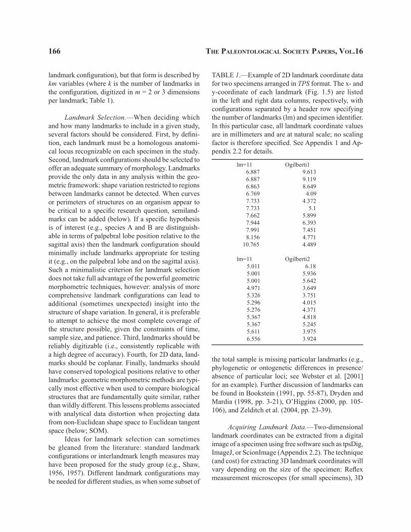
TABLE 1.—Example of 2D landmark coordinate data for two specimens arranged in TPS format. The x- and y-coordinate of each landmark (Fig. 1.5) are listed in the left and right data columns, respectively, with configurations separated by a header row specifying the number of landmarks (lm) and specimen identifier. In this particular case, all landmark coordinate values are in millimeters and are at natural scale; no scaling factor is therefore specified. See Appendix 1 and Ap-pendix 2.2 for details.

lm=11 Ogilberti1 6.887 9.613 6.887 9.119 6.863 8.649 6.769 4.09 7.733 4.372 7.733 5.1 7.662 5.899 7.944 6.393 7.991 7.451 8.156 4.771 10.765 4.489

lm=11 Ogilberti2 5.011 6.18 5.001 5.936 5.001 5.642 4.971 3.649 5.326 3.751 5.296 4.015 5.276 4.371 5.367 4.818 5.367 5.245 5.611 3.975 6.556 3.924

the total sample is missing particular landmarks (e.g., phylogenetic or ontogenetic differences in presence/absence of particular loci; see Webster et al. [2001] for an example). Further discussion of landmarks can be found in Bookstein (1991, pp. 55-87), Dryden and Mardia (1998, pp. 3-21), O’Higgins (2000, pp. 105-106), and Zelditch et al. (2004, pp. 23-39).

Acquiring Landmark Data.—Two-dimensional landmark coordinates can be extracted from a digital image of a specimen using free software such as tpsDig, ImageJ, or ScionImage (Appendix 2.2). The technique (and cost) for extracting 3D landmark coordinates will vary depending on the size of the specimen: Reflex measurement microscopes (for small specimens), 3D


scanners, MicroScribe digitizers, and MRI or CT scans (for large specimens) are potential options.

A key and easily overlooked issue is the quality of the specimen and/or photograph; these will determine the quality of the final data. Reliable landmark data are unlikely to be obtained from a poor-contrast, out-of-focus photograph of a specimen. Do not compromise image quality for speed of data collection! Great at-tention should be paid to maximizing the quality of the specimen and/or photograph prior to digitizing the landmarks. Depending on the study organism, this may include specimen cleaning (e.g., removal of rock matrix), whitening (sometimes preceded by blackening), careful mounting, illumination, and im-age shooting. Image processing software (e.g., Adobe Photoshop) can help enhance a digital image, but will be of limited use if the image is initially out-of-focus or poorly illuminated.

Many taxonomic groups have an established standard orientation for mounting prior to photography or measurement (e.g., Shaw, 1957). The mounting medium used will depend on the size of the specimen. Common options include an SEM stub, toothpick/steel pin (with a temporary adhesive such as gum tragacanth), lead shot, small fishing weights, sand, or modeling clay (although this can leave a residue on the specimen). It is essential to check with museums before preparing and mounting loaned material.

The intricate issues of obtaining a high-quality digital image of a specimen are beyond the scope of this paper, but useful guidelines can be found in Feldmann et al. (1989) and Zelditch et al. (2004, pp. 39-49). Always include a scale bar in the photograph so that the scale of the landmark configuration can be computed. Extracting landmark data from published images offers a quick and easy way to collect data, but has many caveats. It must be assumed that the figured specimen was mounted in the standard orientation, and that the quoted scale is accurate. There is also no guarantee that the specimen was optimally illuminated for extraction of landmark data: some journals have a preference for asymmetrical illumination (e.g., stronger lighting from the upper left) that can create shadows in regions where landmarks are to be digitized. Not all published images will be appropriate for landmark data extraction: a general principle of “if in doubt, throw it out” should be followed.

Landmarks must be digitized in the same order

for all specimens. When collecting data, keep track of any missing landmarks. A specimen with missing data for a landmark cannot be included in an analysis involving that landmark. However, it may be included in other analyses not involving that landmark, and may therefore be worth digitizing.

Semilandmarks.—Semilandmarks are points ar-rayed along an outline that capture information about curvature, making it possible to study complex curv-ing morphologies where landmarks are sparse (Green, 1996; Sampson et al., 1996; Bookstein, 1997; Sheets et al., 2004; Perez et al., 2006). Specialized methods are needed to superimpose semilandmarks (Green, 1996; Sampson et al., 1996; Bookstein, 1997; Andresen et al., 2000; Bookstein et al., 2002; Gunz et al., 2005; below; SOM). However, once superimposed, their coordinates can be analyzed just like those of landmarks (except that semilandmarks have only one degree of freedom; be-low). Incorporation of semilandmarks into a landmark configuration greatly expands the summary of shape, and is becoming increasingly routine in geometric morphometric analyses.

Unlike standard landmarks, semilandmarks are not discrete, anatomical loci and their coordinates are not directly digitized from the specimen. Rather, semilandmark coordinates are calculated from initial curve coordinate data through a complicated procedure (SOM). The logic behind this procedure is that the shape of the curve is biologically interesting, but the number, spacing, and placement of points along the curve is not. Several approaches to reducing the diffi-culties associate with representing a curve by a series of points have been developed. These either minimize the shape difference between forms (Sampson et al., 1996; Sheets et al., 2004; Perez et al., 2006) or produce a series of curves that represent maximally smooth defor-mations of the average curve (Bookstein, 1997). In the first approach semilandmarks are computationally slid along the curve so that their spacing minimally impacts the amount of shape difference between forms (SOM). The coordinates of these optimally slid semilandmarks are incorporated into the final configuration. For 2D data, the location of each semilandmark is specified by two coordinates. However, spacing of semilandmarks along the curve is uninformative: the shape of the curve in the vicinity of a semilandmark is described by the or-thogonal displacement of that semilandmark relative to


a line between its immediately neighboring points. Each semilandmark therefore contributes only one degree of freedom in any comparison. Configurations containing semilandmarks therefore have 2(k + s) variables and 2k – 4 + s degrees of freedom (where k is the number of standard landmarks and s is the number of semiland-marks) when placed in shape space (below). Statistical analysis of configurations that include semilandmarks must therefore be based on nonparametric bootstrap resampling methods (below) or on other approaches where the mismatch of degrees of freedom and number of variables is explicitly taken into account.

Measurement Error.—The process of extracting landmark coordinates will always be associated with some degree of measurement error. This can result from inconsistent tilting (pitch or roll) of specimens relative to the plane of digitization, non-coplanarity of land-marks, and/or difficulty in pinpointing the landmark locus (through biological vagueness, or differences in illumination or focus). Image distortion on the screen (e.g., pixelation) can also introduce non-biological signal. Measurement error can be minimized by careful mounting, photography, and landmark selection, but

can never be totally eliminated. Replicate imaging and digitizing of specimens should be a component of any study: results of among-specimen shape comparison should always be interpreted with respect to within-specimen measurement error (below; Table 2).

suPerIMPosItIon Methods

Having obtained the raw landmark data for a number of specimens, the next step of any analysis is to translate and rotate the landmark configurations into a common position and remove size differences between them. This operation, called superimposi-tion, eases comparison of configurations by removing variation associated with differences in their location, orientation, and size. Such differences are irrelevant in a comparison of configuration shape, because shape is all the geometric information that remains when loca-tion, scale, and rotational effects are filtered out from an object (following the definition by Kendall, 1977). The specialized software available for the analysis of geometric morphometric data will typically handle superimposition internally (Appendix 2.3). However, it is important to understand the issues involved in order

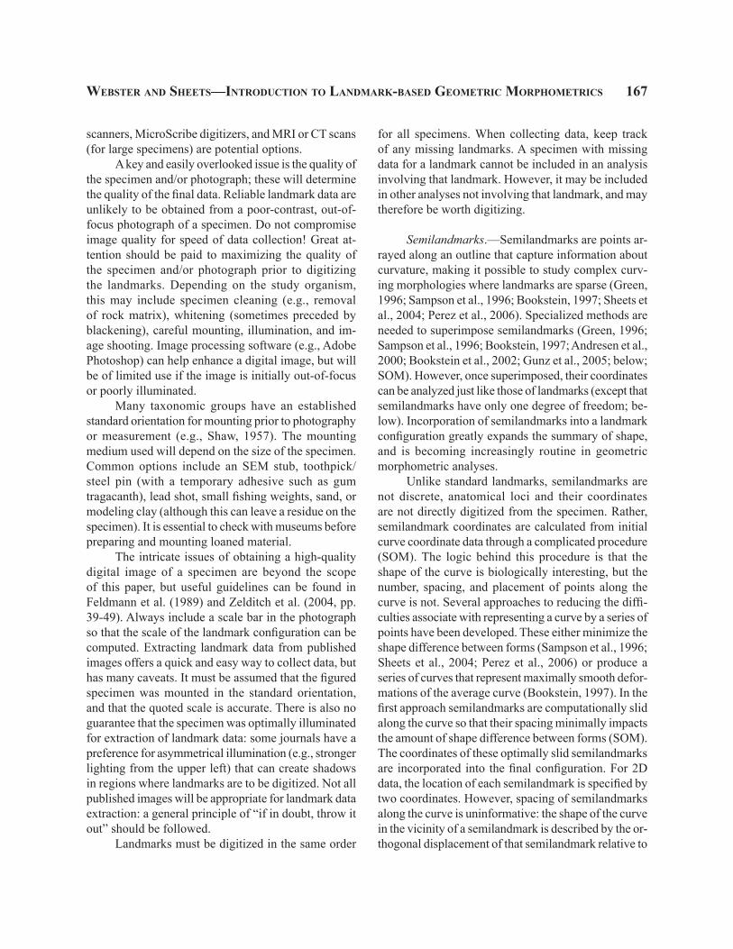
TABLE 2.—Within-species variation, among-species disparity, partial disparity, and measurement error for four species of olenelloid trilobites (Fig. 1). Shape variation for any sample is quantified as average partial Procrustes distance of specimens away from the mean form of that sample (see text for details). Upper and lower confidence limits are based on bootstrap resampling (1600 replicates). Measurement error was assessed for one specimen of Olenellus chiefensis (FMNH PE57383), which was cleaned, mounted, photographed, and dismounted a total of ten times. A landmark configuration was digitized from each of these replicate images, providing an estimate of apparent shape variation associated with measurement error. In this case, measurement error is two orders of magnitude smaller than intraspecific shape variation and is considered negligible. Nevertheless, estimates of variation must be interpreted with caution because biological variation is compounded with compaction-related taphonomic overprint in this particular case study. Species show statistically indistinguishable differences in in-traspecific variation. Partial disparity values reveal that O. chiefensis and O. fowleri make a greater contribution to total among-species disparity than do O. terminatus and O. gilberti. This is consistent with the results of PCA of the total sample (Fig. 5).

n variance Lower 95% Upper 95% Partial Disparity

Olenellus chiefensis error 10 0.000061 0.000029 0.000085 -Olenellus chiefensis 63 0.001799 0.001524 0.002034 0.004475Olenellus fowleri 23 0.002387 0.001554 0.003054 0.004608

Olenellus gilberti 58 0.002377 0.002020 0.002684 0.000662Olenellus terminatus 37 0.001908 0.001544 0.002218 0.001712

Among-species Disparity 181 0.011457 0.010495 0.012524 -


to make reasonable choices about the options offered by such software, and to avoid mistakes when trying to analyze geometric morphometric data with standard statistical tests (below; SOM).

There are several superimposition methods, dif-fering in how and in the degree to which differences in location, scale, and size are removed. Partial Procrustes superimposition is introduced below. Summaries of other superimposition methods (full Procrustes super-imposition, resistant-fit methods, Bookstein registra-tion, and sliding baseline registration), and mathemati-cal details of these methods, are provided in the SOM. The related and equally important issue of shape spaces is discussed in the SOM.

Partial Procrustes Superimposition.—This is the most widely used superimposition method and forms the basis for many subsequent operations in geometric morphometrics (e.g., the thin-plate spline, calculation of warp scores, etc.; below). It is often referred to sim-ply as Procrustes superimposition, a convention that is followed here. Removal of differences in location is achieved by centering configurations. This involves calculating the centroid of each configuration (Text Box 1), and then making the centroid the origin of a new co-ordinate system (SOM). Removal of differences in size between configurations is achieved by rescaling each configuration so that they share a common centroid size of 1 (Text Box 1; SOM). Removal of differences in orientation between two configurations is achieved by rotating one configuration (the target form) around its centroid until it shows minimal offset in location of its landmarks relative to the other configuration (the reference form). The mismatch in landmark locations between the target and reference configurations is quantified as the squared distance between their cor-responding landmarks, summed over all landmarks: the square root of this is the partial Procrustes dis-tance between those configurations (Text Box 2). The two configurations are optimally aligned when this value is minimized (i.e., the rotation produces a least-squares fit; Text Box 2; SOM). (Use of this optimality criterion assumes that variance is equal and circularly [randomly] distributed at each landmark. Resistant-fit superimposition methods can be used if this assumption is grossly violated, although these methods have other substantial disadvantages [SOM].) The procedure of translating all landmark configurations to a common location, rescaling all to unit centroid size, and rotat-

boX 1—centroId and centroId sIZe

The centroid of a configuration is literally its center: the x- and y- (and z-) coordinates of the configuration’s centroid are simply the mean values of the x- and y- (and z-) coordinates for all k landmarks in the configuration.

Centroid size is the square root of the sum of the squared distances between each landmark and the centroid of the form (Bookstein, 1991; this is proportional to the square root of the mean of all squared interlandmark distances). Centroid size is not an immediately intuitive size measure, because the centroid size calculated for any specimen will change if different landmark configurations are used to summarize its shape. (This, of course, is not true for more traditional size measures such as body length, which is constant for any given specimen irrespective of what other variables are measured to summarize its shape.) However, cen-troid size is a useful measure of overall size of a landmark configuration because (1) in the absence of allometry it is mathematically uncorrelated with Kendall’s (1977) definition of shape (i.e., it does not induce a correlation between size and shape in the presence of circular normal landmark errors [see Bookstein, 1991, chapters 4, 5]); and (2) all landmarks in a configuration are equally weighted in the calculation of centroid size, unlike a size proxy such as body length (which is an interland-mark distance and therefore involves only two landmarks in its calculation).

ing all into an optimal least-squares alignment with an iteratively estimated mean reference form is called Gen-eralized Procrustes Analysis (GPA) or, equivalently, or least-squares theta-rho analysis (LSTRA)(Figs. 2, 3.1, 4; Gower, 1975; Rohlf and Slice, 1990; Dryden and Mardia, 1998). Because all differences in location, scale, and orientation have been removed by this proce-dure, any differences in coordinates of corresponding landmarks between configurations must be the result of differences in shape between those configurations.

Procrustes superimposition places configurations in a non-Euclidean shape space, a [km - m - 1 - {m(m - 1)/2}]-dimensional surface of a hypersphere centered


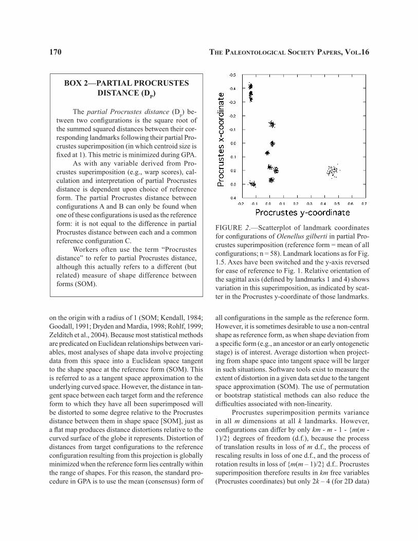
FIGURE 2.—Scatterplot of landmark coordinates for configurations of Olenellus gilberti in partial Pro-crustes superimposition (reference form = mean of all configurations; n = 58). Landmark locations as for Fig. 1.5. Axes have been switched and the y-axis reversed for ease of reference to Fig. 1. Relative orientation of the sagittal axis (defined by landmarks 1 and 4) shows variation in this superimposition, as indicated by scat-ter in the Procrustes y-coordinate of those landmarks.

BOX 2—PARTIAL PROCRUSTES DISTANCE (DP)

The partial Procrustes distance (Dp) be-tween two configurations is the square root of the summed squared distances between their cor-responding landmarks following their partial Pro-crustes superimposition (in which centroid size is fixed at 1). This metric is minimized during GPA.

As with any variable derived from Pro-crustes superimposition (e.g., warp scores), cal-culation and interpretation of partial Procrustes distance is dependent upon choice of reference form. The partial Procrustes distance between configurations A and B can only be found when one of these configurations is used as the reference form: it is not equal to the difference in partial Procrustes distance between each and a common reference configuration C.

Workers often use the term “Procrustes distance” to refer to partial Procrustes distance, although this actually refers to a different (but related) measure of shape difference between forms (SOM).

on the origin with a radius of 1 (SOM; Kendall, 1984; Goodall, 1991; Dryden and Mardia, 1998; Rohlf, 1999; Zelditch et al., 2004). Because most statistical methods are predicated on Euclidean relationships between vari-ables, most analyses of shape data involve projecting data from this space into a Euclidean space tangent to the shape space at the reference form (SOM). This is referred to as a tangent space approximation to the underlying curved space. However, the distance in tan-gent space between each target form and the reference form to which they have all been superimposed will be distorted to some degree relative to the Procrustes distance between them in shape space [SOM], just as a flat map produces distance distortions relative to the curved surface of the globe it represents. Distortion of distances from target configurations to the reference configuration resulting from this projection is globally minimized when the reference form lies centrally within the range of shapes. For this reason, the standard pro-cedure in GPA is to use the mean (consensus) form of

all configurations in the sample as the reference form. However, it is sometimes desirable to use a non-central shape as reference form, as when shape deviation from a specific form (e.g., an ancestor or an early ontogenetic stage) is of interest. Average distortion when project-ing from shape space into tangent space will be larger in such situations. Software tools exist to measure the extent of distortion in a given data set due to the tangent space approximation (SOM). The use of permutation or bootstrap statistical methods can also reduce the difficulties associated with non-linearity.

Procrustes superimposition permits variance in all m dimensions at all k landmarks. However, configurations can differ by only km - m - 1 - {m(m - 1)/2} degrees of freedom (d.f.), because the process of translation results in loss of m d.f., the process of rescaling results in loss of one d.f., and the process of rotation results in loss of {m(m – 1)/2} d.f.. Procrustes superimposition therefore results in km free variables (Procrustes coordinates) but only 2k – 4 (for 2D data)


or 3k – 7 (for 3D data) d.f., which means that standard statistical tests cannot be used to test for difference in shape using Procrustes coordinates (below). (The degrees of freedom differ if the configuration includes semilandmarks; above.)

Another potential drawback of Procrustes su-perimposition is that the orientation of biologically relevant axes is not respected during rotation. For example, unless asymmetry is a focus of interest it is common practice to use landmarks from only one half of a bilaterally symmetrical organism in order to reduce data redundancy (e.g., the examples used here). However, Procrustes superimposition may result in considerable variation in relative orientation of the axis of symmetry within a sample (Fig. 2). This can be inconvenient if differences in shape are to be described in terms of landmark locations relative to the axis of symmetry. Another concern raised about the method is susceptibility to the “Pinocchio Effect”, in which large differences or variances at one or a few landmarks are effectively smeared out over many landmarks by the least-squares rotation (SOM). The least-squares method assumes equal variance at all landmarks, which may not be true generally. Despite these limitations, Procrustes methods are generally the most statistically robust and should be strongly considered in most studies (e.g., Rohlf, 2000, 2003; SOM).

VISUALIZING SHAPE VARIATION

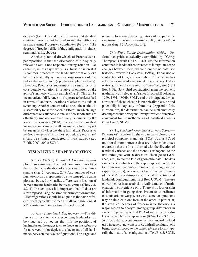
Scatter Plots of Landmark Coordinates.—A plot of superimposed landmark configurations offers the simplest visualization of shape variation within a sample (Fig. 2; Appendix 2.4). Any number of con-figurations can be represented on the same plot. Scatter plots can be used to visualize differences in location of corresponding landmarks between groups (Figs. 3.1, 3.2, 4). In such cases it is important that all data are superimposed using the same superimposition method. All configurations should be aligned to the same refer-ence form (typically the mean of all configurations) if a Procrustes superimposition method is used.

Vectors of Landmark Displacement.—The dif-ference in location of corresponding landmarks can be visualized by vectors that link the positions of landmarks on the target form to those on the reference form. A vector plot depicts displacement of all land-marks between the two configurations. The target and

reference forms may be configurations of two particular specimens, or mean (consensus) configurations of two groups (Fig. 3.3; Appendix 2.4).

Thin-Plate Spline Deformation Grids.—De-formation grids, classically exemplified by D’Arcy Thompson’s work (1917, 1942), use the information contained in landmark coordinates to interpolate shape changes between them, where there are no data (see historical review in Bookstein [1996a]). Expansion or contraction of the grid shows where the organism has enlarged or reduced a region relative to others. Defor-mation grids are drawn using the thin-plate spline (Text Box 3; Fig. 3.4). Grid construction using the spline is mathematically elegant (if rather involved; Bookstein, 1989, 1991, 1996b; SOM), and the interpolated visu-alization of shape change is graphically pleasing and potentially biologically informative (Appendix 2.4). Furthermore, the deformation can be mathematically decomposed into orthogonal “warps” which often prove convenient for the mathematics of statistical analysis (Text Box 3; SOM).

PCA of Landmark Coordinates or Warp Scores.—Patterns of variation in shape can be explored by a principal components analysis (PCA). Just as PCs of traditional morphometric data are independent axes ordered so that the first is aligned with the direction of maximal variance and the second is orthogonal to the first and aligned with the direction of next greatest vari-ance, etc., so are the PCs of geometric data. The data can be the coordinates of the superimposed landmarks (with invariant landmarks removed, if using baseline superimposition), or variables known as warp scores (derived from a thin-plate spline of superimposed landmark configurations; Text Box 3; SOM). The use of warp scores in an analysis is really a matter of math-ematically convenience only. There is no loss or gain of information in going from Procrustes coordinates of landmarks to warp scores, but some computations may be simpler in one form or the other. In particular, the statistical degrees of freedom issue (below) is a major reason to analyze among-group differences in shape using warp scores. A PCA of warp scores is also known as a relative warp analysis (RWA; Figs. 3.5, 3.6, 5). Procrustes superimposition is the standard method used in generating warp scores, with all configurations being superimposed to the same reference form (typi-cally the mean of all configurations; Text Box 3; SOM).


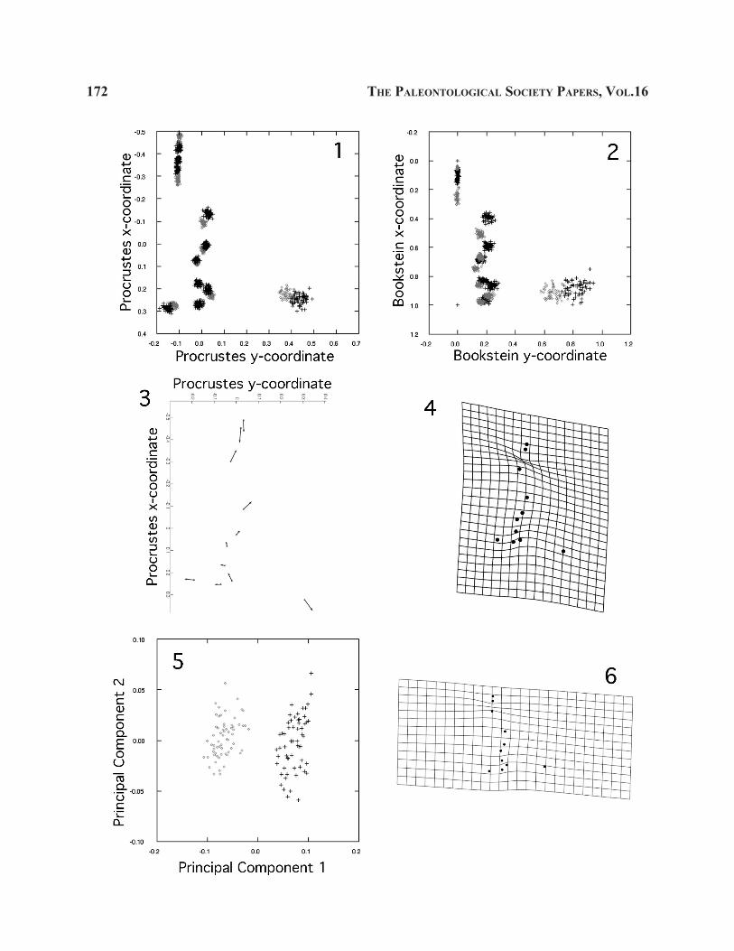
FIGURE 4—Scatterplot of landmark coordinates for configurations of Olenellus gilberti (black crosses; n = 58), O. chiefensis (gray circles; n = 63), O. terminatus (gray squares; n = 37) and O. fowleri (black triangles; n = 23) superimposed using GPA (reference form = mean of all configurations). Landmark locations as for Fig. 1.5. Axes in have been switched and the y-axis reversed for ease of reference to Fig. 1. The most striking inter-specific shape differences (Fig. 1) are evident in these superimposed landmark configurations.

PCA (Appendix 2.4) represents a quick and con-venient way to explore data: outliers (including mis-digitized specimens) and clusters of specimens with similar morphology can be revealed, for example (Figs. 3.5, 5.1, 5.2). It also provides a means of reduction in data dimensionality. In a PCA of Procrustes landmark coordinates, four or seven PCs (for 2D and 3D data, respectively) will have zero eigenvalues due to super-imposition; these PCs can be excluded from subsequent analyses. In any PCA, much of the variance within a sample can typically be explained by relatively few PCs (Figs. 3.5, 5.1, 5.2). Workers familiar with PCA

←FIGURE 3.—1, 2, Scatterplots of landmark coordi-nates for configurations of Olenellus gilberti (black crosses; n = 58) and O. chiefensis (gray circles; n = 63) superimposed using GPA (1; reference form = mean of all configurations) and Bookstein registration (2; baseline = landmarks 1 and 4). 3, Vectors of land-mark displacement showing shape change from mean shape of O. chiefensis to mean shape of O. gilberti (Procrustes superimposition; reference form = mean of all configurations). 4, Thin-plate spline deforma-tion grid showing shape change from mean shape of O. chiefensis to mean shape of O. gilberti (Procrustes superimposition; reference form = mean of all configu-rations). 5, 6, Results of PCA of warp scores (relative warp analysis) of Olenellus gilberti (black crosses; n = 58) and Olenellus chiefensis (gray circles; n = 63); reference form = mean of all configurations. 5, PC1 versus PC2. PC1 explains 75.15% of total variance; PC2 and all higher PCs explain < 8% of total variance and describe trivial aspects of intraspecific variation. 6, Thin-plate spline deformation grid showing shape variation along PC1 in a positive direction. Landmark locations as for Fig. 1.5. Axes in Figs. 3.1-3 have been switched and the y-axis reversed for ease of reference to Fig. 1. Relative to O. chiefensis, O. gilberti is char-acterized by a proportionally shorter preglabellar field (i.e., smaller separation between landmarks 2 and 3), a slightly more anteriorly located posterior tip of the ocular lobe (landmark 10 more anteriorly located), and a proportionally wider cephalon (landmark 11 further from the sagittal axis). The similarity between Fig. 3.6 and Fig. 3.4 confirms that the largest axis of variation among specimens in this total sample relates to inter-specific difference in mean shape.

of traditional data are used to examining axes loadings of the different measurements in a study to determine what the biological importance of PC axes might be, whereas in geometric morphometrics methods the axes encode information about shape change over the entire set of landmarks, and are graphically interpreted as changes in landmark positions (Figs. 3.6, 5.3-5). In particular, it is common to interpret the first PC axis of traditional morphometric data as “size”: this may no longer be as prevalent when working with shape data due to the removal of scale information.

QuantIFyIng and statIstIcally coMParIng the aMount oF

shaPe varIatIon

The magnitude of the difference in shape between two configurations can be quantified by a morphometric distance, the partial Procrustes distance (Text Box 2; SOM). This measure is also useful when quantifying


shape variation within a sample (e.g., intraspecific vari-ation or interspecific disparity), and when statistically testing for differences in mean shape or in variance among samples (e.g., comparisons across age classes or across species). It can also be used to assess mea-surement error by quantifying shape variation across replicates of a single individual (Table 2).

Sample Variation and Disparity.—Variation in shape can be quantified by the average partial Pro-crustes distance of specimens from the sample mean (SOM; Appendix 2.5; Table 2). Bootstrap resampling permits estimation of confidence limits on the observed within-sample variation. The original data set is resa-mpled (with replacement) many times to estimate the range of disparity values possible under resampling. This procedure naturally includes assessment of un-certainty in centroid location (i.e., mean form) of the sample.

The amount of shape variation within one sample can also be statistically compared to that within another based on this bootstrapping procedure. Variation is calculated for each sample separately (as above) and the difference in variation between samples is found by subtraction. Each sample is then resampled (with re-placement) many times, with the variation within each sample and difference in variation between samples be-ing recalculated for each iteration. Confidence intervals for the difference in variation between the samples are calculated from the bootstrapped distribution: if zero is not included within a given confidence interval, then the null hypothesis is rejected at that level of confidence.

Partial Disparity.—Disparity as quantified by the dispersion measure above is sensitive to the distribution of data within the total sample. Addition of a group to a sample can increase or decrease the disparity of the total sample depending on whether the additional group lies far from or close to the grand mean shape of the total sample. Partial disparity (Foote, 1993) is a metric that quantifies the contribution of a particular group to the total morphological disparity of a more inclusive sample (SOM; Appendix 2.5; Table 2). Bootstrap resampling permits estimation of confidence limits on the observed partial disparity. The original data set is resampled (with replacement) many times to generate a distribution of the range of possible partial disparity values. This resampling is done at the specimen (not the group) level, and so includes assessment of the

uncertainty in both the average form of the group and average form of the total sample.

statIstIcal testIng oF dIFFerence In Mean shaPe

Determining whether groups differ in mean shape is a common focus of morphometric analyses. Groups are often delimited by a categorical variable (e.g., spe-cies assignment, sex, geographic locality). Procedures for statistical testing of difference in mean shape with a categorical variable are introduced below (also Ap-pendix 2.6). Some independent variables can be treated as continuously varying covariates (e.g., ontogenetic or stratigraphic absolute age, size). Statistical testing of difference in mean shape with a covariate requires a MANCOVA regression model including an interaction term: space limitations prohibit discussion of such an analysis here (but see Zelditch et al., 2004, pp. 242-248; also Appendix 2.6). Tests based on Procrustes coordinates (and warp scores derived from those) are discussed here. Tests appropriate for coordinates from alternative superimposition methods are mentioned in the SOM.

Tests Based on Procrustes Coordinates.—Pro-crustes superimpostion results in the number of free variables exceeding the number of degrees of freedom (above), so Procrustes coordinates cannot be used as variables in standard multivariate statistical tests of difference in mean shape such as Hotelling’s T2 test or MANOVA. Nevertheless, a nonparametric alterna-tive involving bootstrap resampling (and therefore not demanding estimation of the degrees of freedom) does permit the significance of any difference in mean shape between two groups to be tested (Appendix 2.6; Table 3). This nonparametric test is also appropriate for comparing data that include semilandmarks.

Goodall’s F-test (Goodall, 1991; Dryden and Mardia, 1998; Appendix 2.6; Table 3) is a statistical approach that partitions variance of Procrustes distance rather than of landmark coordinates; it is otherwise analogous to MANOVA. The test measures devia-tions from group and grand means as sums of squared Procrustes distances: Goodall’s F-statistic is the ratio of explained (between-group) to unexplained (within-group) variation in these distances. There are V(G – 1) degrees of freedom for the between-group measure,


boX 3—the thIn-Plate sPlIne and WarP scores

The thin-plate spline (TPS; Bookstein, 1989, 1991, 1996b) is a mathematical model for producing a smooth grid depicting how one shape (the reference form) can be deformed into another (the target form). Warp scores, convenient variables used in many statistical analyses, can be generated through mathemati-cal decomposition of the spline. TPS is a reliable and repeatable mathematical approach to producing the transformation grids introduced by D’Arcy Thompson (1917, 1942). Offset in the locations of corresponding landmarks between the two configurations provides the only data, and the TPS interpolates (using a curve-smoothing spline function) deformation in regions between the landmarks, much in the same way kriging is used to interpolate in other geostatistical applications. Generation of the spline involves elegant matrix algebra (SOM), but can be summarized as follows:

1. One configuration is designated as the “reference form”. The other (“target”) configuration will be compared to this.

2. The target configuration is placed in Procrustes superimposition with the reference form. All non- shape differences between the configurations are therefore removed, and the configurations lie in shape space. Statistical operations can now be carried out in the associated linear tangent space.

3. Vectors of displacement between the superimposed reference and target forms are calculated for each landmark. Each vector has an x- and a y-component.

4. An orthogonal grid is fit over the reference form, “pinned” to it at the landmarks.5. At each landmark, the x-component of the vector of displacement between the reference and tar-

get forms is converted into a vertical displacement of the grid.6. The orthogonal grid is deformed based on the magnitudes of the vertical vectors at the landmarks.

Deformation at all points in the grid not located at the landmark points is interpolated by the spline. Bending of the grid is minimized by a curve-smoothing spline function (see below). The result is that the grid is minimally and smoothly deformed to fit the data.

7. The deformed grid surface is projected back into two dimensions, with the vertical displacements being represented as displacements in the x-direction. Changes in slope of the surface are therefore represented as spatially localized deformations in the x-direction.

8. Steps 4 through 7 are repeated using the y-component of the vector of displacement between the reference and target forms as the vertical displacement, and projecting the deformed grid surface back into two dimensions with the smoothed vertical displacements being represented as displace ments in the y-direction.

Combining the projections produced in steps 7 and 8, a single deformation grid is produced that de-picts how the observed difference in shape between reference and target configurations (i.e., displacement at the landmarks) can be achieved in terms of spatially localized linear deformations. Employment of the curve-smoothing spline function (below) ensures that localized shape change is not interpolated unless the data demand it.

The Curve-Smoothing Spline Function and Bending Energy.—The curve-smoothing spline function serves the critical role of minimizing deformation of the spline surface. It ensures that the smoothest pos-sible topography is maintained as the spline surface is flexed to produce the observed displacement at the landmarks. A summary of how the function operates follows; mathematical details are provided in the SOM.

The deformed grid (spline) is a curved surface, and can be mathematically continuously differentiated: the first derivative being the slope of the surface, the second derivative being the rate of change in slope of the surface. This second derivative is minimized by the smoothing function so that the spline surface passes through each landmark (the data) without introducing unnecessary sharp creases or folds.

By analogy to the deformation of thin, isotropic metal sheets (the mathematical modeling of which


provides the basis for the TPS calculations), the “ease” with which a given amount of vertical deformation is achieved is proportional to the spatial scale over which that deformation is restricted: it requires less “work” to achieve a given amplitude of deformation if the whole surface is allowed to flex than if the flexure is con-strained to occupy only a small portion of the surface. The amount of “work” involved in a given deforma-tion is formally couched in terms of “bending energy”. Bending energy is a function of the arrangement of landmarks on the reference form. Deformations of large spatial scale (i.e., involving differential displacement of landmarks that are widely separated on the reference configuration) require less bending energy than do deformations of a smaller spatial scale (i.e., involving differential displacement of landmarks that are more closely spaced on the reference configuration). Minimizing the second derivative over the entire surface of the spline equates to minimizing bending energy of (and therefore the contribution of spatially localized components to) the total deformation.

Deformations can be split into uniform terms (those which leave parallel lines parallel) and non-uniform terms (those which bend lines that start as parallel lines)(SOM). The TPS method describes all the possible non-uniform deformations of a landmark configuration, but two uniform components (shear and dilation) are also required to form a mathematically complete description of the deformation (SOM). The TPS itself does not include these two factors of shape change, but they are needed to completely describe the differ-ence in shape between the two forms. Most recent discussions refer to warp scores or partial warp scores with the understanding that this also includes the uniform component terms needed to completely describe the deformation. However, some early work in geometric morphometrics drew a distinction between the two types of deformation based on their geometry (affine or non-affine), which seems inappropriate if one is interested in biological causes or factors.

Warp scores are calculated through mathematical decomposition of the TPS (details in the SOM). Each warp score quantifies the contribution of a mathematically independent style of deformation (a warp or one of the two uniform components discussed above) to the shape difference between the reference and target forms. Although the warp scores of any given shape transformation relate to mathematically independent styles of deformation of the reference form, they cannot be treated as biologically independent and should not be analyzed or interpreted in isolation, nor should the uniform components be treated independently of the scores derived from the TPS. In any given shape comparison of 2D data there are 2k – 6 warp scores plus 2 uniform components (SOM) for a total of 2k – 4 variables, which equals the degrees of freedom of the shapes in shape space. (Similarly, there are 3k – 7 warp scores plus uniform terms and 3k – 7 degrees of freedom for 3D data.) This permits standard statistical analyses (e.g., Hotelling’s T2) to be conducted on the full suite of warp scores plus uniform terms to test for the significance of any difference in shape between groups. The warp scores form the variables in a relative warp analysis (see text).

and V(N – G) degrees of freedom for the within-group measure, where V is the dimensionality of shape space (= 2k – 4 for 2-D data or 3k – 7 for 3D data), G is the number of groups, and N is the total number of speci-mens. Goodall’s F-test is useful in that it is a parametric test performed in shape space, so all differences in non-shape factors between forms have been removed. However, variance is assumed to be equal at all land-marks (i.e., the method assumes an isotropic normal distribution of landmark points around the mean). This condition may not be met by empirical data.

Goodall’s F-test is often used as the test statistic for permutation- (Good, 2000) or bootstrap- (Manly,

1997; Efron and Tibshirani, 1998) based tests of dif-ferences in the mean shape of two groups (Appendix 2.6; Table 3). In these approaches, the F-statistic is calculated as discussed above, but then a numerical procedure is used to test for significance (rather than relying on an analytic estimate of the significance of the observed F-value). This avoids the assumption of an isotropic normal distribution of landmark points around the mean (above). In this procedure, the range of F-values obtained by randomly assigning specimens to populations is used to assess the probability that the observed F-value could be due to a random subdivi-sion of an underlying single population. Generalized


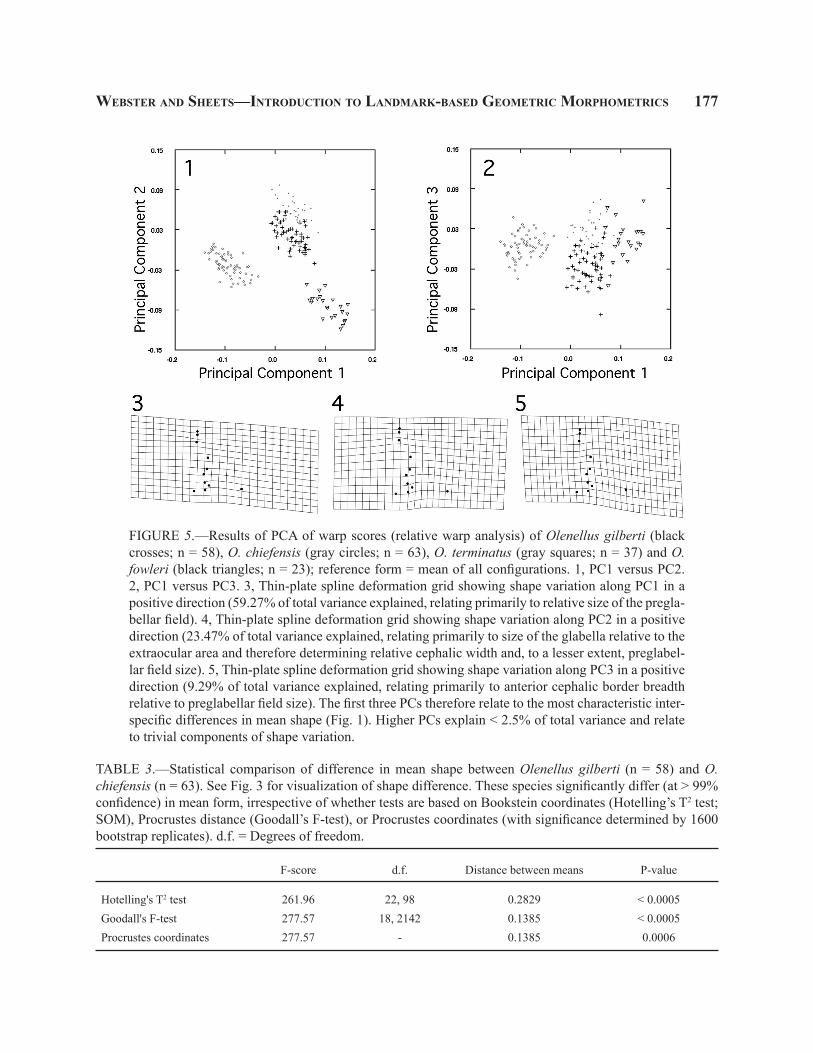
FIGURE 5.—Results of PCA of warp scores (relative warp analysis) of Olenellus gilberti (black crosses; n = 58), O. chiefensis (gray circles; n = 63), O. terminatus (gray squares; n = 37) and O. fowleri (black triangles; n = 23); reference form = mean of all configurations. 1, PC1 versus PC2. 2, PC1 versus PC3. 3, Thin-plate spline deformation grid showing shape variation along PC1 in a positive direction (59.27% of total variance explained, relating primarily to relative size of the pregla-bellar field). 4, Thin-plate spline deformation grid showing shape variation along PC2 in a positive direction (23.47% of total variance explained, relating primarily to size of the glabella relative to the extraocular area and therefore determining relative cephalic width and, to a lesser extent, preglabel-lar field size). 5, Thin-plate spline deformation grid showing shape variation along PC3 in a positive direction (9.29% of total variance explained, relating primarily to anterior cephalic border breadth relative to preglabellar field size). The first three PCs therefore relate to the most characteristic inter-specific differences in mean shape (Fig. 1). Higher PCs explain < 2.5% of total variance and relate to trivial components of shape variation.

TABLE 3.—Statistical comparison of difference in mean shape between Olenellus gilberti (n = 58) and O. chiefensis (n = 63). See Fig. 3 for visualization of shape difference. These species significantly differ (at > 99% confidence) in mean form, irrespective of whether tests are based on Bookstein coordinates (Hotelling’s T2 test; SOM), Procrustes distance (Goodall’s F-test), or Procrustes coordinates (with significance determined by 1600 bootstrap replicates). d.f. = Degrees of freedom.

F-score d.f. Distance between means P-value

Hotelling's T2 test 261.96 22, 98 0.2829 < 0.0005Goodall's F-test 277.57 18, 2142 0.1385 < 0.0005Procrustes coordinates 277.57 - 0.1385 0.0006


BOX 4—CANONICAL VARIATES ANALYSIS

Canonical variates analysis (CVA) determines whether pre-defined groups can be statistically distin-guished based on multivariate data (e.g., warp scores or Bookstein coordinates). In this respect it is analogous to MANOVA, although the mathematics of the two techniques are very different (SOM). CVA is also crudely similar to PCA in that new axes are constructed, each a linear combination of the original variables and or-thogonal to all others, and specimens are then ordered along these new axes. However, each CV is oriented (under the constraints of orthogonality) to summarize the maximal difference between groups (relative to within-group variance) remaining unsummarized by all previous CVs (SOM). CVA therefore fundamentally differs from PCA in that it assumes specimens may be assigned to pre-defined groups, and then tests how well the data (shape in this instance) can be used to support that assignment. (Of course, support may be weak if groups were not originally diagnosed by differences in shape.) Furthermore, CV axes are scaled according to patterns of within-group variation and are not simple rotations of the original coordinate system: a distance between specimens (or groups) in a morphospace defined by CV axes is not necessarily equal to the distance between those same specimens (or groups) in the morphospace defined by the original axes. CVA therefore also differs from PCA in that it efficiently summarizes the description of differences among groups relative to within-group variation (irrespective of how this relates to variation across all specimens).

CVA assumes that all variables are multivariate normal, and that groups share similar variance-covariance structure. In a CVA of k variables measured on specimens assigned to G groups, total sample size must be larger than [(2k – 4) + (G – 1)] in order to obtain a reliable estimate of the variance-covariance structure in the data, and there will be at most (G – 1) distinct canonical axes. In some cases it may not be possible to generate (G – 1) distinct axes, but in such cases the CVA may still reliably assign all specimens.

Wilk’s λ is used to determine how many CVs are statistically distinct from one another. Finding that one or more CVs are significant means that at least some of the groups can be distinguished on those CVs. This does not necessarily mean that all groups can be distinguished; nor does it reveal which of the groups can be distinguished. It also does not describe how effectively the CV axes will discriminate among those groups.

The effectiveness of the CVA in assigning specimens to groups is typically determined using a cross-validation procedure in which a small number of specimens (typically ranging from 1 specimen up to 10% of the population) are omitted from the initial calculation of the CV axes and used as a test set (Appendix 2.7). The omitted specimens are then treated as unknowns and assigned using the CV axes. By repeatedly omit-ting and assigning different test sets, one can obtain the cross-validation assignment rate that should reflect the how well the CVA would assign newly collected specimens to the groups (assuming that the underlying populations were well sampled without bias). When the same specimens are used to create the CVA and to determine the assignment rate, the resulting resubstitution assignment rate will overestimate both the cross-validation rate and the true assignment rate. In a large and robust data set, the cross-validation rate should approach the resubstitution rate.

forms of Goodall’s F-test utilizing partial Procrustes distance may be applied to determine the statistical significance of regression models (Rohlf, 2009b) or in permutation-based MANOVA methods (Anderson, 2001). Goodall’s F-test has been demonstrated to have high statistical power (Rohlf, 2000) and is therefore generally preferred over tests based on Bookstein coordinates (SOM).

Tests Based on Warp Scores.—For 2D data, mathematical decomposition of the thin-plate spline

deformation grid permits reduction of 2k variables (Procrustes coordinates) into 2k – 4 warp scores (in-cluding two uniform terms; Text Box 3; SOM). For 3D data, 3k – 7 warp scores (including uniform terms) are generated. The number of free variables (warp scores plus uniform terms) then matches the degrees of free-dom by which configurations can differ in shape space, so standard statistical procedures (e.g., Hotelling’s T2 test, MANOVA; also canonical variates analysis [CVA; Text Box 4]) can then be applied to determine the


TABLE 4.—Results of statistical testing of group assignments for total sample of 181 cephala of olenelloid tri-lobites based on CVA of partial warp scores plus uniform terms (reference form = mean of all configurations). See Figs. 4, 5, and 6 for visualizations of shape difference. In this test, based on the cross-validation assignment rate (Text Box 4), one specimen of Olenellus gilberti is statistically closer to O. terminatus in terms of cephalic shape; all other a priori species assignments are statistically supported. Statistical testing based on the less desir-able resubstitution assignment rate (Text Box 4) finds complete agreement between a priori species identification and statistical species assignment based on shape similarity (not shown).

Statistical Assignment

O. chiefensis O. gilberti O. terminatus O. fowleri

A Priori Assignment

O. chiefensis 63 0 0 0O. gilberti 0 57 1 0O. terminatus 0 0 37 0O. fowleri 0 0 0 23

FIGURE 6.—Results of CVA of warp scores of Olenellus gilberti (black crosses; n = 58), O. chiefensis (gray circles; n = 63), O. terminatus (gray squares; n = 37) and O. fowleri (black triangles; n = 23); reference form = mean of all configurations. Three distinct canonical variates (CVs) were recovered (all with p < 0.0001). 1, CV1 versus CV2. 2, CV1 versus CV3. 3, Deformation grid showing shape change along CV1 (eigenvalue = 37.50) in a positive direction, relating primarily to size of preglabellar field and location of posterior tip of ocular lobe. 4, Deformation grid showing shape change along CV2 (eigenvalue = 11.04) in a positive direction, relating primar-ily to size of the glabella relative to the extraocular area and therefore determining relative cephalic width and preglabellar field size. 5, Deformation grid showing shape change along CV3 (eigenvalue = 3.64) in a positive direction, relating primarily to breadth of anterior cephalic border. The similarity between these three CVs and the first three PCs (Fig. 5) confirms that the largest axes of variation among specimens in this total sample relate to axes of statistically significant interspecific differences in mean shape.


significance of any shape difference between groups (Appendix 2.6, 2.7; Table 3; Fig. 6). (This does not hold true for warp scores derived from configurations that included semilandmarks.) In any analysis of warp scores, all configurations must be superimposed to the same reference form.

statIstIcal assIgnMent oF sPecIMens to grouPs

CVA (or multi-axis discriminant function analy-sis) can be used to test for significant differences in shape among groups (above) and to determine the confidence with which a priori specimen classification is supported by shape data (Text Box 4; Appendix 2.7; Table 4). (Strong support is not necessarily expected, because a priori group assignments are often not based on among-group shape difference.) The method can also be used to assign unclassified specimens to pre-defined groups, assuming that the specimen actually be-longs in one of the pre-defined groups (Appendix 2.7). Statistical group assignment is based on the distance (D) between the specimen and a group mean (SOM): the predicted group membership of a specimen is the group mean from which it has the lowest D.

concludIng reMarKs

Geometric morphometric approaches form a dazzling component of the toolkit of comparative (paleo)biologists. They offer a powerful and sophis-ticated array of tools that permit an unrivalled ability to simultaneously visualize and statistically quantify differences in form. Thanks to the ever-increasing ease of digitally acquiring landmark data and the availability of free and user-friendly software packages, geometric morphometric studies are becoming more frequent in the paleontological literature. Given the quantitative rigor of geometric morphometric approaches, we expect to see this trend continue and even accelerate. We are also hopeful that geometric morphometric analyses will become an expected component of publications in systematic paleontology and in empirical studies of phenotypic evolution and descriptive/comparative ontogeny. Adopting such a mindset would certainly help exorcise the specter of speculation that has haunted these fields in the past.

acKnoWledgMents

We thank Gene Hunt and John Alroy for the invitation to write this contribution. Two anonymous reviewers and Gene Hunt provided helpful, construc-tive comments on the manuscript. Much of the material presented herein was developed from portions of gradu-ate courses on morphometrics taught by MW at the University of Chicago and as part of the Paleobiology Database Intensive Workshop in Analytical Methods.

REFERENCES

AdAms, d. C., F. J. RohlF, And d. E. sliCE. 2004. Geometric morphometrics: ten years of progress following the ‘revo-lution’. Italian Journal of Zoology, 71:5-16.

AndERson, m. J. 2001. A new method for non-parametric mul-tivariate analysis of variance. Austral Ecology, 26:32-46.

AndREsEn, P. R., F. l. BookstEin, k. ConRAdsEn, B. ERsBøll, J. mARsh, And s. kREiBoRg. 2000. Surface-bounded growth modeling applied to human mandibles. IEEE Transactions in Medical Imaging, 19:1053–1063.

BookstEin, F. l. 1986. Size and shape spaces for landmark data in two dimensions. Statistical Science, 1:181-242.

BookstEin, F. l. 1989. Principal warps: Thin-plate splines and the decomposition of deformations. IEEE Transactions on Pattern Analysis and Machine Intelligence, 11:567-585.

BookstEin, F. l. 1991. Morphometric Tools for Landmark Data: Geometry and Biology. Cambridge Univeristy Press, 435 p.

BookstEin, F. l. 1996A. Biometrics, biomathematics and the morphometric synthesis. Bulletin of Mathematical Biol-ogy, 58:313-365.

BookstEin, F. l. 1996B. Standard formula for the uniform shape component in landmark data, p. 153-168. In L. F. Marcus, M. Corti, A. Loy, G. J. P. Naylor, and D. E. Slice (eds.), Advances in Morphometrics. NATO ASI Series A: Life Sciences Volume 284. Plenum Press, New York.

BookstEin, F. l. 1997. Landmark methods for forms without landmarks: morphometrics of group differences in outline shape. Medical Image Analysis, 1:97-118.

BookstEin, F. l., A. P. stREissguth, P. d. ssAmPson, P. d. Con-noR, And h. m. BARR. 2002. Corpus callosum shape and neuropsychological deficits in adult males with heavy fetal alcohol exposure. Neuroimage, 15:233-251.

ChAtFiEld, C., And A. J. Collins. 1980. Introduction to Multi-variate Analysis. Chapman and Hall/CRC, Boca Raton, Florida, 246 p.


ClAudE, J. 2008. Morphometrics With R. Springer, New York, 316 p.

dRydEn, I. L., And k. V. mARdiA. 1998. Statistical Shape Analy-sis. John Wiley and Sons, Chichester, England, 347 p.

EFRon, B. And R. J. tiBshiRAni. 1998. An Introduction to the Bootstrap. Chapman and Hall, London, 436 p.

EElEwA, A. m. t. (ED.). 2004. Morphometrics: Applications in Biology and Paleontology. Springer-Verlag, Berlin, 263 p.

FEldmAnm, R. m., R. E. ChAPmAn, And J. t. hAnniBAl (EDS.). 1989. Paleotechniques. Paleontological Society Special Publication Number 4, 358 p.

FootE, M. 1993. Contributions of individual taxa to overall morphological disparity. Paleobiology, 19:403-419.

good, P. 2000. Permutation Tests. Second Edition. Springer, New York, 270 p.

goodAll, C. 1991. Procrustes methods in the statistical analysis of shape. Journal of the Royal Statistical Society, Series B (Methodological), 53:285-339.

gowER, J. C. 1975. Generalized Procrustes analysis. Psy-chometrika, 40:33-50.

gREEn, W. D. K. 1996. The thin-plate spline and images with curving features, p. 79-87. In K. V. Mardia, C. A. Gill and I. L. Dryden (eds.), Image Fusion and Shape Variability. University of Leeds Press, Leeds.

Gunz, P., P. mittERoECkER, And F. l. BookstEin. 2005. Semi-landmarks in three dimensions, p. 73–98. In D. E. Slice (ed.), Modern Morphometrics In Physical Anthropology. Kluwer Academic Publishers/Plenum, New York.

kEndAll, d. g. 1977. The diffusion of shape. Advances in Applied Probability, 9:428-430.

kEndAll, d. g. 1984. Shape manifolds, Procrustean metrics, and complex projective spaces. Bulletin of the London Mathematical Society, 16:81-121.

lAwing, A. m., And P. d. Polly. 2010. Geometric morpho-metrics: recent applications to the study of evolution and development. Journal of Zoology, 280:1-7.

mAClEod, N. 2002. Geometric morphometrics and geological shape-classification systems. Earth-Science Reviews, 59:27-47.

mAnly, B. F. J. 1997. Randomization, Bootstrap and Monte Carlo Methods in Biology. Second Edition. Chapman and Hall, London, 399 p.

mARCus, l. F., m. CoRti, A. loy, g. J. P. nAyloR, And d. E. sliCE (EDS.). 1996. Advances in Morphometrics. NATO ASI Series A: Life Sciences Volume 284. Plenum Press, New York, 587 p.

o’higgins, P. 2000. The study of morphological variation in the hominid fossil record: biology, landmarks and geometry. Journal of Anatomy, 197:103-120.

PAlmER, A. R. 1998. Terminal Early Cambrian extinction of the Olenellina: Documentation from the Pioche Formation, Nevada. Journal of Paleontology, 72:650-672.

PEREz, s. i., V. BERnAl, And P. n. gonzAlEz. 2006. Differences between sliding semi-landmark methods in geometric morphometrics, with an application to human craniofacial and dental variation. Journal of Anatomy, 208:769-784.

RiChtsmEiER, J. t., V. B. dElEon, And s. R. lElE. 2002. The promise of geometric morphometrics. Yearbook of Physi-cal Anthropology, 45:63-91.

RiChtsmEiER, J. t., s. R. lElE, And t. m. ColE iii. 2005. Land-mark morphometrics and the analysis of variation, p. 49-69. In B. Hallgrímsson, and B. K. Hall (eds.), Variation: A Central Concept in Biology. Elsevier Academic Press, Burlington, MA, 568 p.

RohlF, F. J. 1990. Morphometrics. Annual Review of Ecology and Systematics, 21:299-316.

RohlF, F. J. 1998. On applications of geometric morphometrics to studies of ontogeny and phylogeny. Systematic Biol-ogy, 47:147-158.

RohlF, F. J. 1999. Shape statistics: Procrustes superimpositions and tangent spaces. Journal of Classification, 16:197-223.

RohlF, F. J. 2000. Statistical power comparisons among alterna-tive morphometric methods. American Journal of Physical Anthropology, 111:463-478.

RohlF, F. J. 2003. Bias and error in estimates of mean shape in geometric morphometrics. Journal of Human Evolu-tion, 44:665-683.

RohlF, F. J. 2008. TPSUTIL. Version 1.40. Department of Ecology and Evolution, State University of New York. Available at <http://life.bio.sunysb.edu.morph/>.

RohlF, F. J. 2009A. tpsDig. Version 2.14. Department of Ecology and Evolution, State University of New York. Available at <http://life.bio.sunysb.edu.morph/>.

RohlF, F. J. 2009B. tpsRegr. Version 1.37. Department of Ecology and Evolution, State University of New York. Available at <http://life.bio.sunysb.edu.morph/>.

RohlF, F. J., And F. l. BookstEin (EDS.). 1990. Proceedings of the Michigan Morphometrics Workshop. University of Michigan Museum of Zoology Special Publication Number 2, Ann Arbor, Michigan, 380 p.

RohlF, F. J., And l. F. mARCus. 1993. A revolution in morpho-metrics. Trends in Ecology and Evolution, 8:129-132.

RohlF, F. J., And d. sliCE. 1990. Extensions of the Procrustes method for the optimal superimposition of landmarks. Systematic Zoology, 39:40-59.

Roth, V. l., And J. m. mERCER. 2000. Morphometrics in devel-opment and evolution. American Zoologist, 40:801-810.


sAmPson, P. d., F. l. BookstEin, h. shEEhAn, And E. l. Bolson. 1996. Eigenshape analysis of left ventricular outlines from contrast ventriculograms, p. 131-152. In L. F. Marcus, M. Corti, A. Loy, G. J. P. Naylor and D. E. Slice (eds.), Advances in Morphometrics. Nato ASI Series, Series A: Life Science, New York.

shAw, A. B. 1956. Quantitative trilobite studies I. The statisti-cal description of trilobites. Journal of Paleontology, 30:1209-1224.

shAw, A. B. 1957. Quantitative trilobite studies II. Measurement of the dorsal shell of non-agnostidean trilobites. Journal of Paleontology, 31:193-207.

shEEts, h. d., k. kim, And C. E. mitChEll. 2004. A combined landmark and outline-based approach to ontogenetic shape change in the Ordovician trilobite Triarthrus becki, p. 67-82. In Elewa, A. M. T. (ed.), Morphometrics: Ap-plications in Biology and Paleontology. Springer-Verlag, Berlin.

sliCE, D. E. 2007. Geometric morphometrics. Annual Review of Anthropology, 36:261-281.

smAll, C. G. 1996. The Statistical Theory of Shape. Springer Series in Statistics. Springer, New York, 227 p.

thomPson, D. W. 1917. On Growth and Form. Cambridge University Press.

thomPson, D. W. 1942. On Growth and Form. A New Edition. Cambridge University Press, 1116 p.

wEBstER, M. 2007. Ontogeny and evolution of the Early Cambrian trilobite genus Nephrolenellus (Olenelloidea). Journal of Paleontology, 81:1168-1193.

wEBstER, M., And N. C. hughEs. 1999. Compaction-related deformation in Cambrian olenelloid trilobites and its implications for fossil morphometry. Journal of Paleon-tology, 73:355-371.

wEBstER, M., And M. L. zElditCh. 2005. Evolutionary modifica-tions of ontogeny: heterochrony and beyond. Paleobiol-ogy, 31:354-372.

wEBstER, M., And M. L. zElditCh. 2008. Integration and regulation of developmental systems in trilobites, p. 427-433. In I. Rábano, Gozalo, R., and García-Bellido, D (eds.), Advances In Trilobite Research. Cuadernos del Museo Geominero 9. Instituto Geológico y Minero de España, Madrid.

wEBstER, M., H. D. shEEts, And N. C. hughEs. 2001. Allometric patterning in trilobite ontogeny: testing for heterochrony in Nephrolenellus, p. 105-144. In M. L. Zelditch (ed.), Beyond Heterochrony: The Evolution of Development. Wiley and Sons, New York.

wEBstER, M., R. R. gAinEs, And N. C. hughEs. 2008. Mi-crostratigraphy, trilobite biostratinomy, and depositional environment of the “Lower Cambrian” Ruin Wash La-gerstätte, Pioche Formation, Nevada. Palaeogeography, Palaeoclimatology, Palaeoecology, 264:100-122.

whitE, C. A. 1874. Preliminary report upon invertebrate fossils collected by the expeditions of 1871, 1872, and 1873, with descriptions of new species. U. S. Geographic and Geologic Surveys West of the 100th Meridian Report. Pp. 5-27.

zElditCh, M. L., D. L. swidERski, H. D. shEEts, And W. L. Fink. 2004. Geometric Morphometrics of Biologists: A Primer. Elsevier Academic Press, San Diego, 443 p.

aPPendIX 1: case study

The morphometric data analyzed in the examples herein were extracted from a diverse assemblage of olenelloid trilobites from the latest Dyeran (traditional Laurentian “Lower Cambrian”) Ruin Wash Lagerstätte, a deposit unusual in its preservation of abundant articu-lated trilobites (Palmer, 1998; Webster et al., 2008). All specimens have experienced compaction-related deformation. The degree of morphological variation exhibited by each species therefore bears a strong ta-phonomic overprint and cannot be taken to represent an accurate measure of biological variation (Webster and Hughes, 1999). Nevertheless, the abundance and otherwise high preservational quality of the material (Fig. 1) make this assemblage convenient for applica-tion of the morphometric techniques introduced herein.

A total of 18 landmarks (four on the sagittal axis and seven abaxial pairs; Fig. 1.5) were digitized on internal molds of cephala of Olenellus gilberti (n = 58), O. chiefensis (n = 63), O. terminatus (n = 37), and O. fowleri (n = 23). Specimens are housed in the collections of the Institute for Cambrian Studies, De-partment of the Geophysical Sciences, University of Chicago (ICS), the Field Museum, Chicago (FMNH), the University of California, Riverside (UCR), and the Cincinnati Museum Center (CMC). All included cephala are morphologically mature (> 5 mm glabel-lar length); for the purposes of the present paper we pretend that growth above this size was isometric for each species so that shape variation is not compounded by ontogenetic shape change, as methods to model on-togenetic changes are beyond the scope of the current paper. Coordinates of abaxial landmarks from the left side of the cephalon were computationally reflected across the midline (defined by landmarks 1 and 4) and their new coordinates averaged with their paired homologues on the right side of the cephalon. This resulted in a total of 11 landmarks per configuration.


This reflecting and averaging procedure reduces data redundancy (appropriate when left-right asymmetry is of little interest, as in these compacted fossils) and also increases sample size (because specimens that are missing one member of a pair of abaxial landmarks can still be included in the analysis; the coordinates of the single member of the landmark pair are used in lieu of the average of the pair). Landmark configurations were arranged in TPS format (Appendix 2; Table 1). The data files and ancillary material needed to run the analyses shown in this chapter can be downloaded through the supplemental online material (SOM).

aPPendIX 2: hoW-to guIde For conductIng landMarK-based

MorPhoMetrIc analyses

We now present a practical guide showing how the exploratory and confirmatory techniques discussed in the paper can be performed in free morphometrics software. The mathematical details of those methods, plus additional geometric morphometric issues, are discussed in the supplementary online material (SOM).

2.1 Morphometric Software Sources on the Web

Morphometric software can be downloaded free of charge from many sites. Perhaps the most widely-used resource is that run by Jim Rohlf at the Stony Brook campus of the State University of New York (<http://life.bio.sunysb.edu/morph/>), which offers ac-cess to a wide array of digitizing and analytical software and example data sets, as well as links to sites run by other morphometricians.

Another useful resource for analytical soft-ware is the site run by HDS (<http://www3.canisius.edu/~sheets/moremorph.html>), from which the latest software releases of the Integrated Morphometrics Package (IMP) can be downloaded. The IMP is a suite of programs, each performing specific morphometric operations or analyses. The programs share a common format and can read each other’s output files. Individu-ally or in combination these programs offer the ability to perform a diverse range of analyses, including all those discussed in a introductory text book to landmark-based geometric morphometrics (Zelditch et al., 2004) and the more limited subset highlighted in the present paper. (Note that older versions of the software, includ-

ing those used by Zelditch et al. [2004], are archived at <http://www3canisius.edu/~sheets/morphsoft.html>. The IMPBasics download from that site does not in-clude the latest software releases.)

The MorphoJ software package developed by Chris Klingenberg at the University of Manchester (<http://www.flywings.org.uk/MorphoJ_page.htm>) and the Morpheus program produced by Dennis Slice at the University of Vienna (<http://www.morphometrics.org/id6.html>) are also popular. Morphologika (<http://sites.google.com/site/hymsfme/downloademorphologi-ka>) and PAST (<http://folk.uio.no/ohammer/past>) are also freely available software packages with limited morphometric capabilities.

Given our intimate familiarity with the IMP software and its intuitive, push-button operation, the following how-to guide focuses on performing mor-phometric analyses in that system. Many of the same analyses could be performed in software available through the SUNYSB site, in MorphoJ, Morpheus, or R (Claude, 2008).

Most IMP programs contain features that are not discussed here. These features pertain to analyses not covered in the present paper (e.g., relevant to ontoge-netic studies). Details of the basic features discussed herein plus these additional features can be found in the manual for each software package (downloaded as part of the IMP installation). Most notably, space limitations do not permit discussion of the important topic of regression analysis, which may be done in the IMP program Regress6 or Rohlf’s tpsRegr (Rohlf, 2009b). The present guide is not intended to replace the manuals that come with the software.

Computer Requirements.—Most morphometric software (including the IMP) currently runs only on PC systems, although MorphoJ is available for PC or Macintosh platforms. New Macintosh computers (with an Intel processor and using Parallels or Bootcamp packages) can run PC-based morphometric software with neglible effect on speed. VirtualPC will allow PC software to run on older Macintosh computers, but this often slows down operations.

2.2 Data Acquisition

The SUNYSB web site (above) offers links to many free programs for acquiring 2D landmark coordi-nates from digital images. The tpsDig software (version


1 or 2; Rohlf, 2009a) is easy to use, and is the preferred digitizing software of the senior author. tpsDig saves landmark coordinates in TPS format (below) that can be read directly into analytical programs (including IMP). This software can also be used in the initial steps of acquiring semilandmark data (SOM). The versatile utility program tpsUtil (also available at the SUNYSB site; Rohlf, 2008) can be used to specify a directory of digital images from which landmarks will be extracted by tpsDig, and also specify the order in which those images will be examined during digitization. Both run on PC platforms.

Alternatively, landmark coordinates can be digitized from images using ImageJ (Macintosh or PC platforms, available at <http://rsb.info.nih.gov/ij/>) or Scion Image (PC platform), available at <http://www.scioncorp.com/>). Landmark coordinates digitized us-ing either of these programs can be copied and pasted into a spreadsheet program (e.g., Microsoft Excel; Macintosh or PC platform) to create a TPS format file (below). Many programs are sensitive to excess line feeds at the end of the files, so if you have difficulty with a translated or altered file, use a text proces-sor to check for excess (or missing) linefeeds. The “error-trapping” in academically produced software is sometimes limited.

Data File Types.—Landmark data are commonly arranged into one of two formats prior to analysis. In the “TPS” format, landmarks in a configuration occupy successive rows in a matrix of two or three columns (one column each for the x- and y- and [if relevant] z-coordinates of the landmarks). Configurations for all specimens are stacked into the same two or three columns (Table 1). The number of landmarks in the configuration (using the statement “LM = k”, where k is the number of landmarks) must be included in a separate row before the first landmark of each speci-men. Various other pieces of information (e.g., a unique specimen identifier, a scale factor, and the number of digitized curves in the configuration [zero for standard landmark data]) can also be incorporated into the data for each specimen as required. Software such as ImageJ or Scion Image (above) can be made to output landmark coordinates at natural scale (e.g., millimeters away from some arbitrary origin) using the “Set Scale” op-tion, in which case no scale factor need be included in the resulting TPS data file. Conversely, tpsDig (above)

records landmark locations in pixel coordinates away from the origin, and the scale must be determined using the “Set Scale” option in the Image Tools window. The scaling factor is then recorded in the TPS data file after the coordinates of the final landmark for each specimen.

The tpsDig program produces data files in TPS format by default. Many of the programs available for download from the SUNYSB site (above) input data in this format, as can CoordGen in the IMP. The example files for the case study analyzed herein (Appendix 1; Table 1) are also in arranged in TPS format.

The “X1, Y1,… CS” format is an alternative data arrangement used by the IMP software. In this format, coordinates of all landmarks for a single specimen occupy a single row (for 2D data, the x-coordinate of landmark 1 is in the first column; the y-coordinate of landmark 1 is in the second column; the x-coordinate of landmark 2 in the third column; y-coordinate of landmark 2 in the fourth column, etc.). Each row ends with the centroid size (Text Box 1) of the configura-tion for that specimen. The final data matrix contains n rows and (km + 1) columns, where n is the sample size and k is the number of landmarks (each digitized in m dimensions). Files in this format load easily into analytical programs such as Systat, SPSS, and R; they will also be read by MorphoJ if the centroid size col-umn is removed and specimen identifiers are inserted as a first column.

Data files in TPS or X1, Y1,… CS format should be saved as tab- or space-delimited text files prior to input to IMP software. This is easily achieved using Microsoft Excel.

2.3 Performing Superimposition

Virtually all geometric morphometrics software internally perform superimposition of the input land-mark data, and most produce a visual display of the superimposed data. The IMP program CoordGen is particularly flexible in terms of its ability to align, dis-play, and save data using a variety of superimposition methods, and forms the basis for the following example.

Using CoordGen: Loading Data.—The push-buttons grouped within the salmon-colored “Load Data” box can be used to load a landmark data file of most common format types. In the current version of CoordGen data files in TPS format with scale factors


(e.g., as generated by tpsDig) must be loaded using the “Other File Options” pull-down menu bar. Input data are shown in the white graphics window. (The default viewing option is for superimposition using Bookstein registration with landmarks 1 and 2 as baseline end-points: this can be changed as described below.)

Superimposing Data.—The green “Display” box contains push-button options for viewing the landmark data using a variety of superimposition methods, including Procrustes (“Show Procrustes”) and Bookstein Registration (“Show BC”). Several other superimposition methods are also available for viewing, including RFTRA and Sliding Baseline Registration (SOM). The superimposed data are displayed in the white graphics window. The displayed image can be copied to the clipboard (and subsequently pasted into other programs) using the yellow button. The “Figure Options” pull-down menu offers some control over the graphical display.

Baseline endpoints (for the baseline-dependent methods) can be specified in the pale blue “Baseline” box: the effect of changing baseline on observed scat-ter at landmarks can quickly be explored by specifying different baseline endpoints and clicking the “Show BC” display option. Procrustes superimpositions (in-cluding RFTRA) align configurations to a reference form. The default reference form is the mean shape of all configurations in the sample. Other reference forms can be specified using the pale gray “Reference Specification” box. (Use of any reference form other than the mean of all can lead to greater distortion when projecting from shape space into tangent space [see text; SOM].) The computed landmark configuration of the current reference form is shown as red crosses in the graphics window.

Saving Data.—The computed landmark coor-dinates of the superimposed data or of the specified reference form can be saved as a space-delimited data file using the blue “Save Coordinates” or orange “Save Coordinates of Reference” box, respectively. The pale gray “Output File Format” box allows the user to se-lect whether the data should be saved in TPS or in X1, Y1,… CS format, the latter being the default. The saved data files can be opened for use in other IMP programs (these require the X1, Y1,… CS format) or imported into programs such as Microsoft Excel, Systat, SPSS, or R.

2.4 Visualizing Shape Variation

Most geometric morphometrics programs pro-duce a visual display of superimposed data. Choice of program will depend on factors such as the nature of variation being studied (e.g., variation within one group or disparity among groups) and the variables by which shape variation is quantified (e.g., landmark coordinates or principal components).

A scatter plot of landmark coordinates for a single sample in a variety of superimposition methods can be produced in CoordGen (Appendix 2.3). Baseline endpoints and reference form are easily defined and changed, permitting rapid exploration of sensitivity of observed shape variation to these parameters for baseline and Procrustes superimposition methods, re-spectively (SOM). For simultaneous superimposition (i.e., to the same reference form or baseline) and display of scatter of landmark coordinates for two groups or more than two groups, the TwoGroup (Appendix 2.6) or PCAGen (below) programs can be used, respectively.

A plot showing vectors of landmark displacement between the mean forms of two groups, and a thin-plate spline deformation grid depicting the spatially local-ized differences in shape between the mean forms of two groups, are most easily generated in TwoGroup (Appendix 2.6).

Variation within a sample (containing superim-posed data for one or more groups) as summarized by a principal components analysis (PCA) of the warp scores away from a common reference form can be visualized using PCAGen (see below).

Using PCAGen: Loading Data.—A single data file of superimposed landmark coordinates in X1, Y1,…CS format for all specimens (irrespective of group membership) should be created (e.g., using CoordGen, above) and loaded into PCAGen using the “Load File 1” push-button in the blue box. If all specimens belong to one group (or if group membership is unknown or immaterial for the analysis) click the “No Group List” push-button. If specimens have been assigned to more than one group, then a group membership data file must be loaded by clicking the “Load Group Membership List” push-button. The group membership data file is a tab- or space-delimited file consisting of a single column of n numbers specifying the group assignment of each of the n specimens in the landmark data file


(specimens must be listed in the same order in the two files). See the example group code and data files in the SOM.

Visualizing Shape Variation.—Upon loading the data a scatter plot of landmark coordinates of the entire data set appears in the white graphics window, color-coded by group if a group list was loaded. Superim-position methods and graphical display are controlled through the light green “Show Landmarks” box and the “Display Options” or “Axis Controls” pull-down menus, respectively, in a similar fashion to CoordGen (Appendix 2.3). Group means (if appropriate) can be displayed in a variety of superimposition methods using the “More Plots” pull-down menu.

Clicking on the “Show PCA Plot” push-button in the purple box performs a relative warp analysis (RWA). This involves several calculations. First, all configurations are aligned in a Procrustes superim-position to a common reference form. By default this reference form is the mean of all configurations, but the configuration of an alternative reference form (in X1, Y1,… CS format, as can be created in CoordGen [Appendix 2.3]) can be loaded in using the “Load Ref-erence” option in the “File” pull-down menu. Second, partial warps are calculated for the reference form. Par-tial warp scores and uniform terms (Text Box 3; SOM) are then calculated for all configurations. Finally, a PCA of the warp scores and uniform terms is conducted.

Upon completion of the calculations, PCAGen displays specimen scores on the first two relative warp axes in the white graphics window. Alternative axes can be displayed by clicking the “Up” or “Down” push-buttons for the x- and/or y-axes in the purple box, then re-clicking the “Show PCA Plot” push-button. The percent of total variance explained by the displayed axes is also shown. Scree plots of eigenvalues or per-cent variance explained for each PC can be displayed using the “Statistics” pull-down menu. The shape change implied by any partial warp can be visualized as a deformation grid using the push-buttons in the pale gray box below the purple box.

The pinkish box in the lower right corner allows placement of two markers at any place in the PCA plot displayed in the graphics window. Shape difference be-tween theoretical configurations located at each marker can then be visualized by clicking the “Show M2-M1” push-button. Superimposition method and display

format (e.g., vectors of landmark displacement, TPS deformation grid) can be specified using the appropriate menus in the turquoise and pinkish boxes, respectively.

Saving Data.—Partial warp scores (plus uniform terms), PCA scores, and the configuration of the refer-ence form can be saved using the push-buttons in the salmon-colored box below the graphics window. The warp scores are arranged in order of increasing spatial scale in the output file: thus the highest warps (of the smallest spatial scale) are listed in the first columns; the two uniform terms occupy the two columns after the partial warps, and the final column is centroid size. Similarly, the output file of the PCA scores has columns corresponding to the highest PCs (i.e., explaining the least variance) listed first. The final column is PC1: centroid size is not appended.

Any image displayed in the graphics window can be copied to the clipboard (and subsequently pasted into other programs) or saved as an EPS file using the relevant yellow buttons.

2.5 Quantifying The Amount of Shape Variation

The amount of shape variation within a sample (quantified as the average partial Procrustes distance of specimens away from the mean form) and group partial disparities are calculated by the IMP Dispari-tyBox program.

Using DisparityBox: Loading Data.—A data file of superimposed landmark coordinates in X1, Y1,…CS format should be created for each of the groups to be compared. Such files can be created using CoordGen (above). These files are loaded sequentially into Dis-parityBox using the “Load Data Set” push-button in the pale box to the right of the Results Box. The “List Loaded Sets” push-button is useful if confusion arises during loading many group files.

Running the Analysis.—A mean configuration (either of all specimens, or of all group means) is cal-culated using the appropriate “Find Grand Consensus Mean” push-button. The superimposed landmark data and the configuration of the computed mean form are displayed in the top right corner. To calculate the aver-age Procrustes distance from the mean for a particular group, select that group using the options in the “Ac-


tive Set” box then select “Bootstrap Disparity within Group” from the “1-Group Analysis” pull-down menu. Group partial disparities and the total disparity exhib-ited by all groups are calculated by selecting “Bootstrap Geometric Disparity (MD, PD)” from the “Multi-Group Analysis” pull-down menu. For all analyses, the num-ber of bootstraps used can be specified in the “Bootstrap Sets” box and results can be saved using options in the “File” pull-down menu.

2.6 Statistical Testing of Difference in Mean Shape

Goodall’s F-test (both analytical and bootstrap-based varieties) of among-group difference in mean shape based on Procrustes distance, and a nonpara-matric test based on Procrustes coordinates (involving bootstrap resampling) can be performed in TwoGroup (below). Warp scores (including uniform terms) of specimens relative to a common reference form (the mean of all specimens) can be generated in PCAGen (Appendix 2.4) and imported into most statistical soft-ware packages (e.g., Systat, SPSS, R) for analysis of among-group difference in mean form using a Hotell-ing’s T2 test or MANOVA. (See Chatfield and Collins [1980], Dryden and Mardia [1998], and Zelditch et al. [2004] for mathematical details of these tests). A CVA of warp scores can be performed in the IMP program CVAGen (Appendix 2.7).

MANCOVA and other regressions of shape vari-ables (including two-way designs) can be performed using the program tpsRegr (Rohlf, 2009b; available from the SUNYSB site, above). Such analyses fall beyond the scope of the present paper.

Using TwoGroup: Loading Data.—A data file of superimposed landmark coordinates in X1, Y1,…CS format should be created for each of the two groups to be compared. (If visualization of shape difference be-tween two particular specimens is of interest, then each group should comprise of duplicated data of a single specimen.) Such files can be created using CoordGen (Appendix 2.3). These files are loaded sequentially into TwoGroup using the blue “Load Data Set 1” and the red “Load Data Set 2” push-buttons.

Visualizing Shape Variation.—Upon loading the data a scatter plot of landmark coordinates of the two groups appears in the white graphics window. Land-

marks are color-coded by group (blue for group 1, red for group 2). Push-buttons in the green box below the graphics window allow visualization of the data in ei-ther Procrustes, Sliding Baseline Registration (“SBR”), or Bookstein Registration (“BC”) superimposition; baseline endpoints can be specified in the orange bar to the right of the graphics window. A scatter plot of landmark coordinates of the mean configuration for each group can be displayed using the push-buttons in the pale blue box below the graphics window (color-coding and superimposition options as above).

Shape difference between group means can be visualized in a variety of modes using options in the purple box. Push-buttons to the left allow the polarity of shape difference to be specified (i.e., whether the mean of group 1 or 2 is the reference form). The su-perimposition method by which the group means are aligned can be specified from the “Superimposition” menu. The “Plot Style” menu allows specification of the visualization mode, including options for vectors of landmark displacement and a thin-plate spline de-formation grid. Other visualization tools (not discussed herein) can be explored. The “Symbols Controls” and “Difference Plot Options” pull-down menus offer some control over the graphical display.

Running Statistical Tests.—Parametric tests (Ho-telling’s T2 test and Goodall’s F-test) are conducted by clicking the appropriate push-button in the pink box. Nonparametric tests based on bootstrap resampling are conducted by clicking on the appropriate push-button in the light green box. The number of bootstraps used can be specified in the “No. of Bootstraps” box. Results appear in the text box.

2.7 Statistical Assignment of Specimens to Groups

The IMP program CVAGen can be used to con-duct a canonical variates analysis (Text Box 4) on warp scores (including uniform terms) to test for significant axes of variation along which pre-defined groups can be discriminated. The program also provides a statisti-cal test of support from shape data for a priori group assignments (Text Box 4; SOM) and can statistically assign unclassified specimens to pre-defined groups.

Using CVAGen: Loading Data.—A single data file of superimposed landmark coordinates in X1, Y1,…


CS format for all specimens (irrespective of group membership) should be created (e.g., using CoordGen, Appendix 2.3) and loaded into CVAGen using the “Load File 1” push-button in the blue box. A group membership data file must then be loaded by clicking the “Load Group Membership List” push-button. (For-mat of this file is discussed under PCAGen; Appendix 2.4.) The “File” pull-down menu also contains an op-tion for loading landmark coordinates of unclassified specimens (as a separate file; a separate group list for these unclassified individuals must also be loaded). These files must be loaded after running the CVA.

Running the Analysis.—Upon loading the data a scatter plot of landmark coordinates of the entire data set appears in the white graphics window, color-coded by group. Control over superimposition method and graphical display is identical to PCAGen (Appendix 2.4).

Clicking on the “Show CVA Plot” push-button in the purple box performs a CVA of partial warp scores and uniform terms (see text). This involves several calculations. First, all configurations are aligned in a Partial Procrustes superimposition to a common reference form. By default this reference form is the mean of all configurations, but the configuration of an alternative reference form (in X1, Y1,… CS format, e.g., created in CoordGen, above) can be loaded in using the “Load Reference” option in the “File” pull-down menu. Second, partial warps are calculated for the reference form. Partial warp scores and uniform terms (Text Box 3; SOM) are then calculated for all configurations. Finally, a CVA of the warp scores and uniform terms is conducted.

Specimen scores on the first two CV axes are displayed in the white graphics window. Alternative axes can be displayed by using the “Up” or “Down” push-buttons for the x- and/or y-axes in the purple box, then re-clicking the “Show CVA Plot” push-button. Eigenvalues of the displayed axes are also shown. Tests of significance, groupings by CV, and assignment tests (below) can be displayed using the “Statistics” pull-down menu. Significance tests are all based on Wilk’s λ and the Bartlett’s test. Test results appear in an Aux-iliary Results Box. The shape change implied by any CV can be visualized as a deformation grid using the push-buttons in the pale gray box below the purple box.

The pinkish box in the lower right corner allows

placement of two markers at any place in the CVA plot displayed in the graphics window. This works in a similar fashion to the analogous box in PCAGen (Appendix 2.4).

Statistical Support from Shape Data for Group Assignments.—Assignment tests (Text Box 4) can be conducted and displayed using the “Statistics” pull-down menu, which allows calculation of both the resubstitution rates (“Show Groupings by CVA” option) and the cross-validation rates (“Jack-knife Groupings” option). Results are presented as a matrix of assignments: specimen assignments made by the user (i.e., in the Group Membership List) are given in the rows, specimen assignments based on the distance D (SOM) are given in the columns. If user and statistical assignments are congruent then all elements will along the major diagonal; non-zero off-diagonal elements indicate lack of statistical support from shape data for a priori group assignment (e.g., Table 4).

Statistical group assignments of unclassified specimens (if any were loaded, above) are given as a separate row (“u”) below the matrix. (These unclassi-fied specimens were not included in computation of the CV axes.)

Saving Data.—Partial warp scores (plus uniform terms), CVA scores, and the configuration of the refer-ence form can be saved using the push-buttons in the salmon-colored box below the graphics window. The warp scores are arranged in order of increasing spatial scale in the output file: thus the highest warps (of the smallest spatial scale) are listed in the first columns. The two uniform terms occupy the two columns after the partial warps, and the final column is centroid size. The output file of the CVA scores has columns corre-sponding to the lowest CVs (i.e., explaining the most variance) listed first. Centroid size is not appended. Statistical group assignments (based on resubstitution rates) can be saved using the “File” pull-down menu.

a PractIcal IntroductIon to landMarK-based geoMetrIc...

Documents

Transcript of a PractIcal IntroductIon to landMarK-based geoMetrIc...