A Practical Guideto

Rotor DynamicsMALCOLM E. LEADER, P.E.

Applied Machinery Dynamics Company

IntroductionRotor dynamics is a very interesting

and complicated subject. The importance ofthis subject has increased over the last fewdecades as machine speeds have increased andhigher flows and efficiencies have had the sideeffect of introducing problems with criticalspeeds, unbalance response and rotor stability.Some of these problems are related to theeconomics of the capital expenditures where amachine may be bought on a cost basis. Fartoo often this results in excessive andexpensive rebuilds and costly lost production.This paper will introduce the basics of rotordynamics and lead into some of the moreadvanced concepts. The mathematics will bekept to a minimum and as many helpful "rulesof thumb" will be included as this subjectallows. Units are shown in detail for eachequation.

At times, rotor dynamics can be a verycontroversial subject from the nomenclatureused to the question of the degree of accuracyneeded to model a rotor dynamic system.There have been many simplifications andassumptions made in this paper and the authoroffers some opinions that some people maydisagree with, but the approach here is quiteconservative and has proven successful overthe last 25 years of my career. The approachesand guidance offered here are based onexperience of many people and many years ofanalyzing and testing machinery. Analyticaland actual test data will be used as examples.

A nomenclature page is included and

whenever possible, the symbols used forvarious factors are identified in the body of thepaper. At the end of the paper is a list ofreferences that the author has found veryvaluable and are recommended for furtherreading.

Rules of thumb are fine but the readershould come to the conclusion that the onlyway to do a meaningful rotor dynamicsanalysis on a machine train will be to procurethe necessary computer programs to do theanalysis. Some sources for programs used inthe preparation of this paper are noted in theacknowledgments. There are many sources forcomputer programs that will run well onpersonal computers. While some are easier touse than others and some use differinganalytical techniques, like any tool, theseprograms are dependent on the skills of theuser. GIGO remains a problem today and themore powerful the program, the more pitfallsthere are waiting. Thus, the main purposes ofthis paper are to introduce the basic concepts ofrotor dynamics and to serve as a reality checkguide. I always ask myself at each stage ofanalysis ”...can that be right?” and if it fitslogically, I proceed. If not, I backup andexamine the input or my assumptions.

Basic ConceptsA compressor rotor, pump impeller,

steel structure and a tuning fork all havesomething in common: they all haveresonances. When a tuning fork is struck, itemits a tone (actually many tones, but oneprincipal tone). Strong winds may "ring" abuilding's natural frequencies or cause largemotions on a bridge. A rotor may have itsnatural frequencies excited by many sources:rotating imbalance, rubs, or process changessuch as surge. The first objective of rotordynamics is to identify the resonantfrequencies present in a system, determine theirseverity and, if necessary, design the systemaround them. A typical machinery train mayconsist of a driver, a gear and a driven such as

a compressor. It is not atypical to have 10 ormore system resonances to design around. Sohow does one begin? Do you need acomplicated computer analysis to identify theseresonances and do a complete system analysis?The answer is, yes, you probably do, however,there are many things that can be looked atquickly and easily with an eye toward generaltrends and design practices. In some cases, thismay suffice, particularly if the vendor iscapable of good rotor dynamics analysis, andmost are.

A rotor, supported in bearings of somesort, is analogous to the familiar spring-mass-damper system shown in figure 1.

Figure 1 - SPRING-MASS-DAMPER

The governing equation for the motion of sucha system is:

It is absolutely crucial to understand theimplications of this equation. It means that theforcing function (which in a rotating elementusually means the imbalance forces but can beother things like misalignment, rubs,aerodynamic forces, etc.) is opposed by onlythree things: the system inertia (mass), thesystem damping and the system stiffness.These three things are frequency dependent.At low frequencies, below resonance, thestiffness is the primary control. When thefrequency of a forcing function coincides with

a natural frequency of the rotor, we encounterwhat is commonly called a critical speed forrotating equipment. Here the damping controlsthe motion. At high frequencies, the inertiatends to control motion. This is analogous tovibration measurements where displacementsensors are most sensitive at lower frequenciesand accelerometers are most sensitive at higherfrequencies.

If we ignore the damping term for themoment and set the forcing function to zero wefind that the solution of the equation gives thefirst natural frequency:

Note that damping is not included in thisequation. We will add the effects of dampinglater when we consider fluid film bearings.

This solution is not directly applicableto all rotor systems as we shall see. In a simpleexample, shown in figure 2, consider a singlemass rotor with a rigid shaft supported onidentical bearings:

Figure 2 - Simple rigid shaft system

However, a rigid shaft is not normally areasonable assumption, and many shafts havemore than one mass, either between bearings oroverhung. Thus we must first find the shaftstiffness from beam theory.

For a circular shaft:

So, for example, let’s envision a very simplecase without external weights and without anyoverhung sections. I chose a 5 inch diametershaft with a span of 80 inches. The stiffness ofthis shaft is:

Now, to include this in the previous examplewe must recalculate the system stiffness. Theshaft is a spring supported on two other springswe call bearings. Springs in series add likeresistors in parallel, that is inversely. So:

Notice that the system stiffness is always lowerthan any of the components. Thus, our naturalfrequency calculation is now (assuming thatthe total system mass is the same 1,000 LBm):

This is a 255% decrease from the rigid caseshowing that, in this case, shaft stiffness is thedominant factor. This is usually true in mostrotating equipment. This principal wasoriginally developed in 1894 by Dunkerley,who stated that the principle of superpositionapplied to critical speeds in an inverse manner:

Additional information about the mathematicalapproach to rotor dynamics is available inabundance. A few of the best references arelisted at the end of this paper.

To get a feel for a given rotor-bearingsystem, some general rules of thumb can beapplied. The first of these is the concept ofmodal mass. Modal mass can be thought ofas the effective mass "seen" by a particularmode at resonance. For a between bearingsystem at its first critical speed, the modalmass is equivalent to the mass that would yieldan equivalent system if all the mass werelumped in the center of the span. Figure 3 is aplot of modal mass (modal mass/total mass) asa function of the stiffness ratio betweenbearing and shaft stiffness (2Kb/Ks). Thestiffness ratio is very important and greatlyaffects the modal mass ratio among otherthings. As the support stiffnesses becomemuch less than the shaft stiffness, the rotorbegins to behave as a free body and the modalmass becomes equal to the total mass.

Figure 3 - Modal Mass Concept

As the support stiffnesses become much largerthan the shaft stiffness, the modal mass ratioasymptotically approaches 0.5. For mostactual cases that this author has encountered,modal mass ratios between 0.52 and 0.60 havebeen most common. When in doubt, use 0.55.As an example, see figure 4.

Figure 4 - Typical Compressor Rotor

This is an actual propylene refrigerationmachine installed in an ethylene plant.Suppose we need a quick estimate of thismachine's first critical speed so we don'taccidentally run too close to it during a startup.We begin by calculating the shaft stiffness:

The bearings for this rotor are highly preloadedtilting shoe bearings and were calculated tohave a stiffness of 3,500,000 LB/IN each. Soto get the system stiffness we add thestiffnesses inversely:

If we were to use the total rotor mass tocalculate the first critical speed:

But this isn't even close to the actual criticalspeed. So, refer to figure 3 and calculate thestiffness ratio 2Kb/Ks = 7.63. This translatesto a modal mass ratio of 0.56. So our firstcritical speed calculation becomes:

As can be seen in figure 5, the actual firstcritical speed of this machine was between2000 and 2100 RPM. Thus we can see that thismethod works fairly well for between bearingrotors with evenly distributed external masses.

Figure 5 - Actual Compressor Startup

Mode ShapesAssociated with every resonance or

critical speed is a mode shape. Mode shapesare only defined at resonance and areindependent of the forcing function. At anyother speed the rotor simply has a deflectedshape that is due to the proximity of resonancesand forcing function distribution.

Let’s return to the simple 5-inchdiameter shaft selected earlier where theoverall length and bearing span are 80 inches.We’ll examine the effects of changing thesedimensions later. The mode shapes of anyresonance of any rotor are only dependent onthe shaft stiffness, the bearing stiffness, theshaft mass and the mass and distribution of thecomponents mounted on the shaft. Sometimes,due to shrink fits, mounted components canincrease the apparent shaft stiffness. Dampingcontrols the severity of a resonance, not themode shape.

The stiffness ratio, 2Kb/Ks, can be usedas a non-dimensionalizing factor to betterunderstand the behavior of modes shapes.Let’s look at the first three calculated modeshapes of our simple rotor as we vary thebearing stiffness as a function of shaft stiffness.Figure 6 shows how the mode shapes of thefirst three critical speeds change as the stiffness

ratio ranges from 2Kb=Ks to 2Kb =10Ks. Looking at the first critical speed, when

the bearings are relatively soft (2Kb=Ks), therotor has a translational “bouncing” motion upand down with little shaft bending. As thestiffness of the bearings increase, they clampdown on the shaft. More and more bending ofthe shaft appears until there is very littlemotion at the bearings.

The second critical speed has a rockingor pivotal motion with a point of no motion inthe center. This is called a node point. At thatresonant frequency, there is no motion at thatpoint. At low bearing stiffnesses there isvirtually no bending in the rotor but as thestiffness of the supports increases, the secondcritical speed takes on an “S” shape.

The third critical speed is different. Atlow (even zero) bearing stiffnesses, the rotorhas a definite bent shape. This is a free-free or“bearingless” mode and is the lowest frequencyat which the rotor will “ring” when hung andhit with a hammer. As the stiffness of thesupports increases, this basic shape is retainedwith additional deflection at the ends near thebearings. The third critical speed mode shapehas 2 node points regardless of the bearingstiffnesses. The number of nodal points for asimple shaft like this is always the criticalspeed number minus one.

It is an important point that the first twocritical speeds of this type of simple rotorsystem are inherently translational modes.At zero support stiffness they do not exist.Bending is induced in the shaft as the supportsincrease in stiffness but only the third modeand higher are inherently bending modes.This way of referring to criticals speeds iscommonly misused with the first critical speedoften called a bending mode. It is not.

Some machines with very soft supportshave critically damped first and second criticalspeeds: that is, you cannot detect them innormal operation. However, this does notmake the third critical speed (which is almostalways very excitable) suddenly become the

first critical speed. We need to keep ourterminology consis tent for bet terunderstanding.

Indeed, as we will see, reducing theamount of first mode shaft bending is a veryimportant goal. It is easy to see that as shaftbending increases, the critical speed frequencywill increase.

The Critical Speed MapOne of the most useful tools available

to anyone evaluating the rotor dynamics of arotor bearing system is the undamped criticalspeed map. This device allows us tocompletely quantify the possible critical speedsof our machine. It does not necessarily revealanything about the true critical speedfrequencies and it does not predict the severity

of the resonances. It does give a good guidethat can be used to understand how variouschanges in the bearings or shafting will affectthe critical speeds.

Continuing on with the originalexample of a simple shaft, let’s vary thesupport stiffnesses from 1,000 LB/IN to1,000,000 LB/IN and calculate the first threecritical speeds over this entire range. Figure 7shows these calculations on a log-log plot. Thefirst critical speed rises from 400 RPM whenthe bearing stiffness is 1,000 LB/IN to 1,200RPM at 10,000 LB/IN to 2,800 RPM at100,000 RPM and finally 3,600 RPM at 1million LB/IN. At this point this curvebecomes asymptotic and increasing thestiffness of the bearings will not significantlyincrease the first critical speed frequency. One

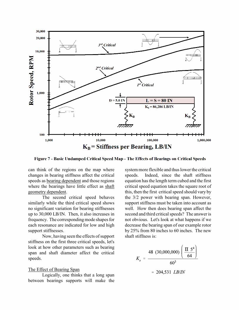
can think of the regions on the map wherechanges in bearing stiffness affect the criticalspeeds as bearing dependent and those regionswhere the bearings have little effect as shaftgeometry dependent.

The second critical speed behavessimilarly while the third critical speed showsno significant variation for bearing stiffnessesup to 30,000 LB/IN. Then, it also increases infrequency. The corresponding mode shapes foreach resonance are indicated for low and highsupport stiffnesses.

Now, having seen the effects of supportstiffness on the first three critical speeds, let'slook at how other parameters such as bearingspan and shaft diameter affect the criticalspeeds.

The Effect of Bearing SpanLogically, one thinks that a long span

between bearings supports will make the

system more flexible and thus lower the criticalspeeds. Indeed, since the shaft stiffnessequation has the length term cubed and the firstcritical speed equation takes the square root ofthis, then the first critical speed should vary bythe 3/2 power with bearing span. However,support stiffness must be taken into account aswell. How then does bearing span affect thesecond and third critical speeds? The answer isnot obvious. Let's look at what happens if wedecrease the bearing span of our example rotorby 25% from 80 inches to 60 inches. The newshaft stiffness is:

Compared to the 80 inch span case stiffness of86,286 LB/IN this is a remarkable increase of137% in shaft stiffness. Figure 8 is anundamped critical speed map showing how thisspan change affects the first three criticalspeeds. The solid lines are the 80 inch spancase and are identical to figure 7. The dashedlines are the critical speeds for the 60 inch spancase. Looking at the first critical speed one cansee that there is an overall increase in the firstcritical speed regardless of support stiffness,but since the mode is purely translational atvery low support stiffnesses, the bearings exertless influence than at higher support stiffnesseswhen bending is introduced. The shorter spaninduces more bending at high supportstiffnesses and thus drives up the first criticalspeed. Above 1,000,000 LB/IN the increase isa constant 70 percent.

The second critical speed behaves

somewhat differently. At low stiffnesses, theshortened bearing span causes a decrease in thesecond critical speed; the two curves cross atabout 500,000 LB/IN support stiffness. Then,for higher stiffnesses, the second critical speedis higher for the shortened span case. At lowstiffnesses this mode is pivotal with maximumamplitudes at the rotor ends and a node point inthe center. Moving the bearings inward movesthem away from the area of maximumamplitude and thus decreases theireffectiveness. It is very important to note thatthe closer to a pivot point (node) the lesseffective a bearing will be. This is the reasonfor the decrease in the second critical speed forthe shortened span case at low supportstiffnesses. As with the first mode, as thebearings "clamp down" on the shaft, increasedbending is induced and the shortened spanincreases the resistance to bending, driving up

the second critical speed.The third critical speed experiences a

similar phenomena. At very low supportstiffnesses the span will have no effectwhatsoever, but as the support stiffness beginsto affect the third mode, the bearings are nowcloser to the 2 node points and thus have areduced effect, lowering the third criticalspeed's frequency.

Thus, changes in bearing span aredependent upon the system's support stiffness.The first critical speed can be effectively raisedby a decrease in span and this method is oftenused to raise the first critical speed out of anoperating range. It will also raise the secondcritical if there is sufficient support stiffness.

The Effect of Shaft DiameterThe other major factor which controls

critical speeds is shaft diameter. Designers ofcentrifugal compressors like small shaftdiameters so that they can make the impellereyes small, bearings small, seals small, keepthe frame size down and the overall designcompact and inexpensive. Since shaft diameteraffects the moment of inertia, I, then the firstcritical should vary by the square root of I.Let's take our example rotor, hold the spanconstant at 80 inches and vary the shaftdiameter by first decreasing it 25% to 3.75inches and then increasing it 25% to 6.25inches. Total rotor weight will vary as thediameter changes (total weight is a function ofshaft radius squared) and you will see that theweight changes have an effect as well as the

shaft diameter changes. Again we must look atthe effect as a function of support stiffness.Figure 9 is the undamped critical speed map

which compares shaft diameters as a functionof support stiffness. The solid line is thebaseline case of 5.0 inch diameter shaft. Thedotted line is the smaller 3.75 inch shaft andthe dashed line is the larger 6.25 inch case.

The first critical speed lines show thatat low support stiffness the smaller diametershaft has a higher first critical speed and thelarger shaft a lower first critical speed. This isbecause the dominant factor with very lowsupport stiffness is the rotor weight. Since theshaft stiffness is not effective when no bendingis taking place, the lighter rotor will raise thefirst critical speed and the heavier rotor willdecrease it. As support stiffness rises, thelogical change occurs and the smaller shaft hasa much lower first critical speed. Since thesmaller diameter shaft is more flexible, thebearing stiffness becomes dominant faster.Notice how this curve "flattens out" muchfaster and approaches an asymptotic value.This more flexible shaft has a smaller bearingdependent region on the critical speed map.The stiffer shaft increases the first criticalspeed at moderate and high support stiffnessesand also does not become asymptotic as fast.The stiffer shaft has a larger bearing dependentregion on the map. Note that, in this case,when the bearing stiffness is about 80,000LB/IN the shaft diameter has little effect on thefirst critical speed.

The second critical speed curves showa response similar to the first critical and forthe same reasons. The mass influence is evengreater and the support stiffness must begreater than about 750,000 LB/IN before thelarger shaft's second critical increases over thebaseline case. The third critical is a bit different in thatat low support stiffnesses, the system isinherently a bending mode and the stiffer shaftwill be more resistant with the larger diameterand have a higher third critical speed.Likewise, the smaller diameter shaft will beless resistant to bending.

Shaft Diameter Effects on a Steam TurbineThe simple shaft example only

illustrates basic ideas. In reality, most rotorshave a significant amount of weight added asimpellers or other disks. Let’s consider anactual steam turbine and vary the shaftdiameter. Figure 10 shows the original rotor.

Figure 10 - Built-Up Turbine Rotor

This machine operated at 3,600 RPM driving agenerator. The bearing span was 66.5 incheswith a major shaft diameter of 6 inches. It wasmounted on very stiff bearings and oftenrubbed while passing through the critical speed.If we take the bearing span and divide by themidspan diameter, the ratio is 11.1 to 1. Thisis an easy calculation to do and we know fromexperience that if this value exceeds 10 to 1 weprobably have a problem machine. One way totame this situation is to use a very soft bearing,but that often is not possible.

Instead, what about making the shaftbigger? Since the disks on this rotor make upa substantial percentage of the total rotorweight, this should mask the effect of theadded shaft weight as we increase the diameter.

Figure 11 shows the effects ofincreasing the midspan diameter to 9 inches fora span/diameter value of 7.4 and to 12 inchesfor a span/diameter of 5.5. Note that the rotorweight increases by only 20 percent for thelargest shaft. The bearing stiffness anddamping values were held constant as was the

imbalance, placed at the rotor center. This wasadjusted to 40W/N for each case.

The amplification factor is defined byAPI as the “sharpness” of the resonance asshown in figure 12:

Figure 12 - API 617 Amplification Factor

The higher the amplification factor, the moreviolent the resonance becomes. In this case theoriginal amplification factor was calculated tobe over 70! Increasing the shaft diameter to 9inches brings this down to a more reasonableamplification factor of 10 but this places thecritical speed too close to the operating speed.By increasing the midspan diameter to 12inches the amplification factor drops to a low4.1 and moves the critical speed well aboveoperating speed. Which turbine would yourather have?

The Effect of Mass DistributionSince masses added to the shaft appear

to have a significant effect, let’s look at somelimiting cases. Taking our original 80 inch longrotor and attach 500 pounds in three ways.First of all would be the uniform distributioncase, such as a multi-wheel compressor with

the stages equally spaced. Then there is thecase of a single mass lumped in the center ofthe span such as a single wheel turbine. Finallyconsider the case where you have two-wheelswith half the total mass lumped at the quarter-span points. Figure 13 shows the critical speedmap for this as we take our example rotor anddistribute 500 pounds as outlined above. Thesolid line is the uniform distribution case, thedotted line is the center-lumped case and thedashed line is the quarter-span lumped case. Inall cases the total rotor mass is identical as is

the shaft diameter of 5 inches.The first critical speed responds by

having the highest critical speed for the quarterspan lumped distribution and the lowest for thecenter-lumped case. This is logical when youthink of the mode shape of the first criticalspeed. The maximum amplitude is at the rotor

center and thus the concentrated mass moreeasily affects the first critical. As the mass isdistributed outward, the mass near the bearingscontributes less to the modal mass and thus thefirst critical speed is raised.

The mass distribution has an oppositeeffect on the second critical speed. Regardlessof stiffness, the center lumped case has thehighest second critical speed of the three cases.This is because of the node point in the centerof the span and this lumped mass cannot exertmuch influence at all. At higher support

stiffnesses the quarter span masses are nearestthe high amplitude points and are effective inlowering the second critical speed.

The third critical speed is againdifferent. The uniform case has the lowestthird critical speed and the quarter span casehas the highest. The mode shapes provide the

explanation. The quarter-span case has themasses close to the node points and thus areineffective, causing an increase in the thirdcritical speed. The center span case puts themass at a point of maximum amplitude and iseffective in lowering the third critical speed,but the uniform case puts mass at all threemaximum, amplitude points and is mosteffective in lowering the third critical speed.

To summarize, mass is effective inlowering critical speeds when it is near amaximum amplitude point. The modal massfor that mode is then increased causing adecrease in the resonant frequency of thatmode. To drive up a critical speed, put theconcentrated mass at a node point where it willnot increase the effective modal mass.

Unbalance Response AnalysisSince imbalance is the most common

excitation factor, one of the important thingswe are interested in when evaluating a rotor-bearing system is how that system will respondto this external forcing function. Many rotorssuffer from the problem of buildup from aprocess residue or erosion and wear. Thus, thebalance when installed may not maintain itself.The question is, what level of imbalance willresult in unacceptable levels of vibration? It isnecessary to introduce damping into theequations of motion to accurately model theunbalance response since damping is the onlymechanism able to absorb energy at resonance.It is necessary to use a computer program tocalculate accurate amplitudes on a rotorbearing system. Unbalance responsecalculation programs are very similar to criticalspeed programs with the addition of a knownforcing function and realistic bearing stiffnessand damping values for the supports. Once thephysical model is constructed, the userspecifies the location and the magnitude of theimbalance and the program calculates thesteady-state response at fixed speed incrementsthroughout a specified speed range. The resultscan be formatted as a Bodé or a polar plot.

Bodé plots are shown in figure 11 and anexample of a polar plot is figure 14. Anothertype of output available from an unbalanceresponse calculation is the operating speeddeflection shape as shown in figure 15. This isvery useful when setting vibration limits sinceit tells you the amplitude at any locationcompared to the vibration probe location.

The first question is how muchimbalance to input into the program and whereto place it on the rotor. The generally acceptedbalance tolerance in wide use today is 4W/N or4 times the rotor weight in pounds divided bythe maximum continuous speed in RPM. Theunits of imbalance are in ounce-inches or OZ-IN. If this level of imbalance is used, thepredicted amplitudes will usually beunrealistically low. Since the calculations arelinear, theoretically any amount could be usedand the results scaled. I prefer to use 40W/N asa worst-case scenario.

To begin an analysis, mode shapes fora rotor are produced using the actual predictedbearing stiffnesses. See figure 6 for examples.Then the entire imbalance is placed at themaximum amplitude point indicated by the firstundamped mode shape to excite the firstcritical speed . For the second critical speed,the 40W/N imbalance is split in two and half isplaced at each end of the rotor 180° out-of-phase with each other and at the maximumamplitude points indicated by the second modeshape. Higher mode excitation will follow asimilar procedure.

In summary, unbalance responsecalculations are not as straightforward asundamped critical speed calculations. Youmust already know something about the modeshapes before you can place the imbalances.Once the results of an unbalance response areobtained, the user can calculate anamplification factor as outlined earlier andbegin to get a feel for the rotor's sensitivity.

Often, based on experience with a givenrotor configuration, an analyst will place acomplex distribution of imbalances on a rotor

(for example at wheel locations, overhangs andcouplings, etc.) in order to excite all pertinentmodes simultaneously.

Stability AnalysisStability analysis is the most difficult

aspect of rotor dynamics. It is not nearly aswell understood as the previously coveredsubjects and the computer programs that areavailable require that the user estimate theamount of destabilizing influences in thesystem. The destabilizing forces are commonlydesignated cross-coupling forces. These cross-coupling forces cause an orthogonal forwarddisplacement of the rotor for each normal rotordisplacement. If the force is sufficient inmagnitude to overcome the damping in thesystem, an instability occurs. Stability is afunction of rotor geometry, bearing-to-shaftstiffness ratio, bearings, seals, and fluiddynamics.

The best measure of rotor stability is thelogarithmic decrement. Often called the logdec for short, this factor is related toamplification factor and is defined as thenatural log of the ratio of two successiveresonant amplitudes. When the log dec ispositive, the systems vibrations die out withtime and the system is stable. However, if thelog dec is less than zero, the system's vibrationsgrow with time and the system is unstable. Therelationship of the log dec, abbreviated “*” toamplification factor is this:

The log dec can be experimentally determinedby momentarily exciting a running rotor at oneof its natural frequencies either by a forcingfunction or an impulse. By recording theresultant "ring-down" the log dec can becalculated. Compressor surge is an excellentexciter (and wrecker) of machinery, but if wellcontrolled this may be used to impulse the rotor

and excite the first critical while running at ahigher speed. This is shown in figure 16 whichis the time trace of an axial compressor'sdisplacement probe signal during a surge test.A log dec of 0.35 can be calculated from thistrace.

System instability is almost alwaysmanifested by the presence of forwardsubsynchronous circular whirling of the shaft ata frequency equal to the first critical speed. Inmost cases the driving mechanism is the fluidfilm in the journal bearings. Two distinctphenomena can occur that are related butdifferent:

Oil Whirl: This is a circular forwardsubsynchronous vibration that nominallyoccurs near 50% of synchronous rotor speedand tracks with rotor speed. To visualize this,consider the oil wedge in the bearing. The oilat the surface of the bearing is at zero speed.The oil at the journal surface is at the shaftsurface speed and the average oil speed is then50% of running speed. This is not entirely truehowever, due to surface roughness differences,the shaft is usually smoother than the bearingand this is why oil whirl often occurs at 42% to48% of rotor speed. If the journal area is veryrough, say due to a rusty shaft, oil whirl can beobserved at frequencies greater than 50% ofsynchronous speed. Oil whirl can be inducedby bushings and seals as well as bearings.Many bearing designs are "anti-whirl" bearingssuch as tilting pad bearings.

Oil Whip: This phenomena is similarto oil whirl, but occurs at a constant frequency.This frequency is almost always the firstcritical speed. The shaft must also be turningat a speed greater than twice the first criticalspeed. Many systems will run very well untilexactly twice the first critical speed is reachedand the rotor will go into violent oil whip. Oilwhip can also be induced by seals and bushingsand it can be controlled in bearings by using amore stable design Whirl and whip can be veryviolent and can destroy a machine in minutes

so it is very important to prevent it at thedesign stage.

One of the first things the designauditor should check is the bearing to shaftstiffness ratio, 2Kb/Ks. As this ratio exceeds avalue of 10, the rotor is starting to become a"noodle" and will be susceptible to instabilities.The use of plain journal bearings in a rotorwhich exceeds twice its first critical speedshould be a warning sign. Floating oilbushings and high pressure labyrinth seals likebalance piston drums should also be looked atas potential cross-coupling sources.

The bearing analysis should lookcarefully at the predicted operating speedeccentricity ratio. If this ratio becomes lessthan 0.2 the likelihood of bearing instabilitiesexist. The reason for this is that a centeredbearing has equal clearance all around and iseasily perturbed from this position. Manybearings counteract this centering phenomenaby inducing an external load on the shaft bypreloading the bearing, or in the case of thepressure dam bearing, the oil itself creates apressure wedge in the upper half of the bearingthat pushes down on the journal, increasing theeccentricity, and the stability. Often you willsee a groove cut in the bottom half of a bearing.This groove reduces the bearing's load carryingcapacity and at the same time increases theeccentricity and the stability. Sometimes aquick fix for an unstable machine is to mill outa pressure dam and/or load groove in the plainjournal bearing. This needs to be done withextreme care as the critical speeds andunbalance response will also be affected bysuch a change.

There are other destabilizing forcescalled aerodynamic cross-coupling. This is afluid induced force around the periphery ofcentrifugal wheels or other rotatingcomponents.

There are semi-empirical equations forestimating the amount of cross coupling. Oneof these was developed by Mr. J. C. Wachel

now retired. For compressible flow:

This equation should be used carefully,particularly in determination of the factor "h".

Figure 17 shows the results of a typicalstability study on a compressor. The log dec iscalculated for several speeds and plotted. Thecross-over point in this case is 7,240 RPMwhich means this is the speed where themachine begins to show signs ofsubsynchronous vibration.

AcknowledgmentsThe following people have helped me

with my understanding of rotor dynamics overmany years. I thank them here: Mr. CharlieJackson, Dr. Edgar J. Gunter, Dr. Gordon Kirk,Dr. John Nicholas, Dr. Paul Allaire, Dr. LloydBarrett, Mr. Buddy Wachel, and others toonumerous to mention.

Some of the computer programs usedby the author have been developed by theROMAC Laboratory at the University ofVirginia. The primary tool used was theDyRoBeS suite of analysis programs developedby Dr. Wen Jeng Chen of Eigen Technologies,Inc. and distributed by RODYN VibrationAnalysis, Inc.

NomenclatureC - damping, LBf-SEC/IN

cC - critical damping, LBf-SEC/IN

E - Young's modulus, PSI

g - Gravitational Constant,386.088 LBm-IN/LBf-Sec2

I - area moment of inertia, IN4

K,k - spring stiffness, LBf/IN

BK - bearing stiffness, LBf/IN

SK - shaft stiffness, LBf/IN

Kyx - Cross-Coupling, LB/IN

M,m - Mass, LBf (mass = weight/g)

N - rotational speed, RPM

Ncx - critical speed number x, RPM

B - 3.14159...

S - Sommerfeld number

T - frequency, RAD/SEC

dT - damped natural frequency,RAD/SEC

nT - undamped natural frequency,RAD/SEC

x - displacement, inches

xN - velocity, inches/second

xO - acceleration, inches/second2

* - logarithmic decrement,dimensionless

c. - damping ratio - C/C ,dimensionless

REFERENCESAPI 617, Centrifugal Compressors for GeneralRefinery Services, F o u r t h E d i t i o n ,November, 1979.

Ehrich, E. F., "Identification and Avoidance ofInstabilities and Self-Excited Vibrations inRotating Machinery", ASME 72-DE-21, May,1972.

Eshleman, R. L., "ASME Flexible Rotor-Bearing System Dynamics, Part 1 - CriticalSpeeds and Response of Flexible RotorSystems", ASME H-42, 1972.

Gunter, E. J., 1966, “Dynamic Stability ofRotor-Bearing Systems”, NASA SP-113, pp153-157

Gunter, E. J., "Rotor-Bearing Stability",Proceedings of the First TurbomachinerySymposium, Texas A&M University, pp. 119-141, 1972.

Jackson, C., The Practical Vibration Primer,Gulf Publishing Co., Houston, TX., FirstEdition, 1979.

Jackson, C., and Leader, M. E., "Rotor CriticalSpeed and Response Studies for EquipmentSelection", Vibration Institute Proceedings,April 1979, pp. 45-50. (reprinted inHydrocarbon Processing, November, 1979, pp281-284.)

Leader, M. E., “Understanding JournalBearings”, Vibration Institute, Annual Meeting,2001.

Lund, J. W., "Stability and Damped CriticalSpeeds of Flexible Rotor in Fluid-FilmBearings", ASME 73-DET-103, Cincinnati,September, 1973.

Lund, J. W., "Modal Response of a FlexibleRotor in Fluid-Film Bearings", ASME 73-DET-98, Cincinnati, September, 1973.

Newkirk, B. L., and Taylor, H. D., “ShaftWhipping Due to Oil Action in JournalBearings”, General Electric Review, 28, pp559-568.

Prohl, M. A., "A General Method forCalculating Critical Speeds of FlexibleRotors", Transactions ASME, Volume 67,Journal of Applied Mechanics, Volume 12,Page A-142.

Reiger, N.F., "ASME Flexible Rotor-BearingDynamics, Part III - Unbalance Response andBalancing of Flexible Rotors in Bearings",ASME H-48, 1973.

Tonnesen, J. and Lund, J.W., "SomeExperiments on Instability of Rotors Supportedin Fluid-Film Bearings", ASME 77-DET-23,Chicago, 1977.

Vance, J . M. “Rotordynamics ofTurbomachinery”, John Wiley & Sons, 1988,ISBN 0-471-80258-1

Weaver, F. L., "Rotor Design and VibrationResponse", AIChE 49C, September, 1971, 70thNational Meeting.