a planning methodology for railway construction cost ...
126
Graduate eses and Dissertations Iowa State University Capstones, eses and Dissertations 2011 a planning methodology for railway construction cost estimation in north america Jeffrey Tyler Von Brown Iowa State University Follow this and additional works at: hps://lib.dr.iastate.edu/etd Part of the Business Commons is esis is brought to you for free and open access by the Iowa State University Capstones, eses and Dissertations at Iowa State University Digital Repository. It has been accepted for inclusion in Graduate eses and Dissertations by an authorized administrator of Iowa State University Digital Repository. For more information, please contact [email protected]. Recommended Citation Von Brown, Jeffrey Tyler, "a planning methodology for railway construction cost estimation in north america" (2011). Graduate eses and Dissertations. 10389. hps://lib.dr.iastate.edu/etd/10389
Transcript of a planning methodology for railway construction cost ...

Graduate Theses and Dissertations Iowa State University Capstones, Theses andDissertations
2011
a planning methodology for railway constructioncost estimation in north americaJeffrey Tyler Von BrownIowa State University
Follow this and additional works at: https://lib.dr.iastate.edu/etd
Part of the Business Commons
This Thesis is brought to you for free and open access by the Iowa State University Capstones, Theses and Dissertations at Iowa State University DigitalRepository. It has been accepted for inclusion in Graduate Theses and Dissertations by an authorized administrator of Iowa State University DigitalRepository. For more information, please contact [email protected].
Recommended CitationVon Brown, Jeffrey Tyler, "a planning methodology for railway construction cost estimation in north america" (2011). Graduate Thesesand Dissertations. 10389.https://lib.dr.iastate.edu/etd/10389

i
A planning methodology for railway construction cost estimation
in North America
by
Jeffrey Tyler von Brown
A thesis submitted to the graduate faculty
in partial fulfillment of the requirements for the degree of
MASTER OF SCIENCE
Major: Transportation
Program of Study Committee:
Konstantina Gkritza, Co-Major Professor
Reginald Souleyrette, Co-Major Professor
Michael Crum
Iowa State University
Ames, Iowa
2011

ii
Table of Contents
List of Figures ...................................................................................................................................... iv
List of Tables ........................................................................................................................................ v
Acknowledgements ............................................................................................................................ vii
Abstract ............................................................................................................................................... viii
Chapter 1 - Introduction ...................................................................................................................... 1
1.1 Research Objectives ................................................................................................................ 1
1.2 Anticipated Benefits .................................................................................................................. 2
1.3 Organization of this Thesis ...................................................................................................... 3
Chapter 2 - Literature Review ............................................................................................................ 4
2.1 Overview of the Railroad Industry .......................................................................................... 4
2.2 Freight Demand: Past, Current, and Future Trends ............................................................ 5
2.3 Passenger Demand: Future Trends ..................................................................................... 13
2.4 High Speed Rail Systems ...................................................................................................... 15
2.6 Review of Cost Estimation Methods .................................................................................... 23
Chapter 3 - Methodology Overview ................................................................................................ 27
3.1 Methodology Components ..................................................................................................... 27
3.2 Influencing Factors .................................................................................................................. 31
3.2.1 Location Characteristics ................................................................................................. 31
3.2.2 Service Characteristics ................................................................................................... 37
3.3 CPM Components ................................................................................................................... 41
3.5 Demonstration of the CPM Methodology ............................................................................ 53
3.6 Methodology Notes ................................................................................................................. 56
Chapter 4 - CPM Estimation Results .............................................................................................. 57
4.1 Results Overview .................................................................................................................... 57
4.2 Validation of the CPM methodology ..................................................................................... 62
4.2.1 Individual CPM Comparison............................................................................................... 62
4.2.2 Categorical CPM Comparison ........................................................................................... 71
4.2.2.1 Categorical Cost Comparison Results ...................................................................... 75
Chapter 5 – Conclusions, Limitations and Recommendations ................................................... 78

iii
5.1 Conclusions .............................................................................................................................. 78
5.2 Limitations and Recommendations ...................................................................................... 79
Appendix A ......................................................................................................................................... 82
Appendix B ......................................................................................................................................... 86
Appendix C ......................................................................................................................................... 94
Appendix D ......................................................................................................................................... 99
Bibliography ...................................................................................................................................... 113

iv
List of Figures
Figure 2-1: Mode Market Share as a Percentage of Intercity Ton-Miles (adapted from
(Cambridge Systematics, 2005)) ....................................................................................................... 6
Figure 2-2: Miles of Railroad and Tons Originated (1955-2005) (Weatherford, et al., 2008) .. 7
Figure 2-3: Trains-Miles per Track-Mile for Class I Railroads, 1978 to 2004 (CBO, 2006) ..... 8
Figure 2-4: 2005 Level of Service (Base Line) (Cambridge Systematics, Inc, 2007) ............. 10
Figure 2-5: 2035 Level of Service (without investment) (Cambridge Systematics, Inc, 2007)
.............................................................................................................................................................. 11
Figure 2-6: 2035 Level of Service (with investment) (Cambridge Systematics, Inc, 2007).... 12
Figure 2-7: Emerging Mega Regions of the U.S. (Hagler, et al., 2009) .................................... 13
Figure 2-8: Designated HSR and other passenger rail routes (Federal Railroad
Administration, 2011) ........................................................................................................................ 15
Figure 2-9: US High Speed Rail Association 4 Phase National HSR Rail System (US High
Speed Rail Association, 2011)......................................................................................................... 18
Figure 2-10: 110 - mph Non-Electric Study Cost Distribution ..................................................... 25
Figure 3-1: CPM components and corresponding influencing factors....................................... 30
Figure 3-2: Terrain distribution by state ((U.S. Geological Survey) (ESRI Press, 2008)) ...... 32
Figure 3-3: Terrain distribution by state ......................................................................................... 33
Figure 3-4: Land use distribution by state ...................................................................................... 35
Figure 3-5: Original U.S. Census population density for influencing factor (U.S. Census
Bureau, 2011) ..................................................................................................................................... 36
Figure 3-6: Modern General Electric locomotive (General Electric) .......................................... 41
Figure 3-7: Modern Siemens AG electric locomotive (Buczynski, 2010) .................................. 41
Figure 3-8: Railway track maintenance cost as a function of speed (Adapted from
(Thompson, 1986)) ............................................................................................................................ 47
Figure 4-1: Summary of “Build” 220-mph Single Track ............................................................... 59
Figure 4-2: Double Track CPM Estimates by Service Type ........................................................ 60
Figure 4-3: Example of 220-mph Categorical Cost Changes ..................................................... 61
Figure 4-4: Individual Cost Comparison: 110 - mph Non-Electric .............................................. 65
Figure 4-5: Individual Cost Comparison: 125 - mph Non-Electric .............................................. 66
Figure 4-6: Individual Cost Comparison 125 - mph Electric ........................................................ 67
Figure 4-7: Individual Cost Comparison 150 - mph Electric ........................................................ 68
Figure 4-8: Individual Cost Comparison 220 - mph Electric ........................................................ 69
Figure D-1: Individual Cost Comparison 110 - mph Non-Electric – Graph ............................... 99
Figure D-2: Individual Cost Comparison 125 - mph Non-Electric - Graph .............................. 102
Figure D-3: Individual Cost Comparison 125 - mph Electric – Graph ..................................... 104
Figure D-4: Individual Cost Comparison 150 - mph Electric – Graph ..................................... 107
Figure D-5: Individual Cost Comparison 220 - mph Electric – Graph ..................................... 109

v
List of Tables
Table 2-1: Freight Rail Traffic, 1998 and 2020 (adapted from (CBO, 2006)) ............................. 9
Table 3-1: Summary of Existing CPM Studies ......................................................................... 28-29
Table 3-2: State Terrain Classification Table ................................................................................ 34
Table 3-3: State Land Use Classification Table ............................................................................ 35
Table 3-4: CWCCIS State Adjustment Factors (adapted from (U.S. Army Corps of
Engineers, 2000)) ......................................................................................................................... 43-44
Table 3-5: CWCCIS Feature Code and yearly cost indexes (adapted from (U.S. Army Corps
of Engineers, 2000) ...................................................................................................................... 44-45
Table 3-6: ROW Calculation: 79 & 110 – mph Single Track Urban ........................................... 49
Table 3-7: ROW Costs: Urban Land Use (Adjusted for state influence) ................................... 49
Table 3-8: Material Cost Categories ............................................................................................... 51
Table 3-9: C&S Infrastructure Information ..................................................................................... 52
Table 3-10: Electric Infrastructure Information .............................................................................. 53
Table 3-11: 110 – mph Upgraded Single-Track Non-Electric railway in Suburban Hills ........ 54
Table 3-12: 150 – mph Built Double-Track Electric railway in Suburban Plains ...................... 55
Table 4-1: “To Build” Single Track Plains CPM Estimates .......................................................... 57
Table 4-2: “To Build” Single Track Hills CPM Estimates ............................................................. 58
Table 4-3: “To Build” Single Track Mountains CPM Estimates .................................................. 58
Table 4-4: Summary Statistics of Study Costs (n = 77) .......................................................... 63-64
Table 4-6: Individual Cost Comparison: Statistics (n = 77) ......................................................... 69
Table 4-7: Cost Category Comparison Example .......................................................................... 72
Table 4-8: Sensitivity Analysis Results – 150-mph Electric ........................................................ 73
Table 4-9: Parameter Sensitivity Analysis Comparison – 220-mph Electric ............................ 74
Table 4-10: Comparison of Categorical CPM Estimates ........................................................ 75-77
Table A-1: ROW Calculation: 79 & 110 – mph Single Track Urban .......................................... 82
Table A-2: ROW Proportion Calculations: Urban ......................................................................... 83
Table A-3: ROW Proportion Calculations: Suburban ................................................................... 83
Table A-4: ROW Proportion Calculations: Rural ........................................................................... 84
Table A-5: ROW Costs: Urban Land Use (Adjusted for state influence) .................................. 84
Table A-6: ROW Costs: Suburban Land Use (Adjusted for state influence) ............................ 85
Table A-7: ROW Costs: Rural Land Use (Adjusted for state influence) .................................... 85
Table B-1: CPM to Build Single Track Plains ................................................................................ 86
Table B-2: CPM to Build Single Track Hills ................................................................................... 87
Table B-3: CPM to Build Single Track Mountains ........................................................................ 87
Table B-4: CPM to Build Double Track Plains .............................................................................. 88
Table B-5: CPM to Build Double Track Hills .................................................................................. 88
Table B-6: CPM to Build Double Track Mountains ....................................................................... 89

vi
Table B-7: CPM to Build Additional Track Plains.......................................................................... 89
Table B-8: CPM to Build Additional Track Hills ............................................................................. 90
Table B-9: CPM to Build Additional Track Mountains .................................................................. 90
Table B-10: CPM to Upgrade Single Track Plains ....................................................................... 91
Table B-11: CPM to Upgrade Single Track Hills ........................................................................... 91
Table B-12: CPM to Upgrade Single Track Mountains ................................................................ 92
Table B-13: CPM to Upgrade Double Track Plains ...................................................................... 92
Table B-14: CPM to Upgrade Double Track Hills ......................................................................... 93
Table B-15: CPM to Upgrade Double Track Mountains .............................................................. 93
Table C-1: Parameter Sensitivity Analysis Comparison – 110-mph .......................................... 94
Table C-2: Parameter Sensitivity Analysis Comparison – 125-mph .......................................... 95
Table C-3: Parameter Sensitivity Analysis Comparison – 125-mph Electric ............................ 96
Table C-4: Parameter Sensitivity Analysis Comparison – 150-mph Electric ............................ 97
Table C-5: Parameter Sensitivity Analysis Comparison – 220-mph Electric ............................ 98
Table D-1: Individual Cost Comparison Statistics: 110 - mph Non-Electric ............................. 99
Table D-2: Individual Cost Comparison 110 - mph Non-Electric Data ............................. 100-101
Table D-3: Individual Cost Comparison Statistics: 125 - mph Non-Electric ........................... 102
Table D-4: Individual Cost Comparison: 125 - mph Non-Electric - Data................................. 103
Table D-5: Individual Cost Comparison Statistics: 125 - mph Electric .................................... 104
Table D-6: Individual Cost Comparison: 125 - mph Electric - Data .................................. 105-106
Table D-7: Individual Cost Comparison Statistics: 150 - mph Electric .................................... 107
Table D-8: Individual Cost Comparison: 150 - mph Electric - Data ......................................... 108
Table D-9: Individual Cost Comparison Statistics: 220 - mph Electric .................................... 109
Table D-10: Individual Cost Comparison: 220 - mph Electric – Data ............................... 110-112

vii
Acknowledgements
I would like to thank Louis S. Thompson for information regarding his past
work on railroad studies, and Mark Amfahr, for his recommendations and time
regarding the review of the material. I would also like to recognize the support from
my friends and family. And most importantly, I would like to thank Dr. Konstantina
Gkritza, Dr. Reginald Souleyrette, and Dr. Michael Crum, for their guidance and
advice on this research and my time at Iowa State University.

viii
Abstract
The railroad industry is expected to see increased demand in the United
States (U.S.) over the next 30 years. This demand will put a strain on the
infrastructure and its ability to provide timely and efficient service. Various
technologies are currently available to increase railroad capacity, but in time new
trackage will either need to be added to existing routes, built as new routes, or
existing routes be upgraded to a higher speed classification. Anticipating these costs
is a challenge, since few railroad miles are constructed annually and there are
various factors affecting costs. However, it is possible to calculate cost per mile
(CPM) accounting for right-of-way (ROW), design and build, materials,
communications and signaling, and electrification, where applicable. This thesis
presents a methodology for estimating CPM of railroad construction in the U.S. as a
function of design speed, geography, land use, number of tracks, and motive power.
The proposed CPM estimates were compared to CPM estimates from feasibility
studies, and resulted in the majority of costs being replicated by the methodology.
The proposed methodology has been developed in an adaptable manner, where
future project cost components may be included, creating a dynamic estimation
methodology for analysis and planning activities, prior to feasibility study analyses.

1
Chapter 1 - Introduction
The railroad industry is expected to see increased demand in the United
States (U.S.) over the next 30 years (Cambridge Systematics, 2005) (Cambridge
Systematics, Inc, 2007) (CBO, 2006) (Weatherford, et al., 2008). This demand will
put a strain on the railroad infrastructure and its ability to provide timely and efficient
service. Various technologies are currently available to increase capacity, but in time
new trackage will either need to be added to existing routes, built as new routes, or
existing routes upgraded to a higher speed classification. Anticipating these costs is
a challenge, since few railway miles are constructed annually and the numerous
variables involved mean that each is different from another. However, it is possible
to calculate cost per mile (CPM) estimates accounting for right-of-way, the design
and build, materials, communications and signaling, and electrification, where
applicable.
This thesis presents a methodology for estimating the CPM of railway
construction in the U.S. for use in planning analysis and activities. These estimates
make it possible to anticipate costs for current or future routes based on the top
speed, terrain, land use, number of tracks, and motive power.
1.1 Research Objectives
The objective of this research is to develop a railway construction CPM
estimation methodology that accounts for major factors affecting design, while being
available in a simple and adaptable format. This research is meant to provide

2
transportation planners and policy makers with a systematic process for estimating
costs that are representative of the area and service in question, for analysis and
decision making purposes. This methodology is not meant to replace the depth and
detail of feasibility studies or professional railroad planning activities, but rather to be
used as an intermediate tool to allow planners to more easily perform railroad
analysis and planning activities on their own, prior to contracting out feasibility
studies.
1.2 Anticipated Benefits
Predicting the exact costs of railway construction is very difficult, if not
impossible. But being able to determine realistic and representative estimates based
on influencing factors that will factor into the cost of the railway, will allow a wider
range of analysis to be performed by planning personnel and therefore shorter time
to satisfy decision making deadlines concerning network and service demands. The
proposed CPM estimation methodology would be used as one of the first steps in
the planning process. Due to the capital intensiveness of a railroad construction
project, preliminary estimates of project costs can help to determine whether
planning for such a project would be beneficial. The CPM methodology is not
intended to replace the use of feasibility studies that provide the accurate cost
estimates as well as ridership and economic impacts. But rather, the CPM
methodology could be used as a qualifier for project advancement in the planning

3
process, and may help the planning entity utilize resources and funds more
efficiently.
1.3 Organization of this Thesis
This thesis is organized as follows: Chapter 2 includes a literature review
documenting the need for capacity enhancements from freight and passenger traffic,
capacity improvements currently available, as well as current methods of cost
estimation and their associated benefits and challenges. Chapter 3 discusses the
factors that influence the cost of railway construction and the resulting cost
components defined as design criteria used to capture those influences. Chapter 4
discusses the results of the methodology, including trends and patterns as exhibited
by select design criteria. Chapter 5 includes a comparison, validation, and
discussion of the estimation methodology with individual and categorized study
costs. Lastly Chapter 6 offers the conclusions and limitations of this research, as
well as recommendations for further research.

4
Chapter 2 - Literature Review
2.1 Overview of the Railroad Industry
The current railroad network in the United States (U.S.) is the product of 180
years of development (Armstrong, 2008). Specifically, today’s network is the result of
an industry-wide contraction in the last 60 years, where mergers, abandonments,
and consolidations have taken a former network of some 250,000 route miles in
1916 to roughly 120,000 as of 2010 (Armstrong, 2008). As a result the industry has
tailored operations for efficient transportation of the current levels of demand, but
may not be capable of supplying the capacity to meet future demand. It is common
to encounter different descriptions of the structure upon which rail operations are
performed, the most common being a railroad or railway. To simplify the use of
these terms, the American Railway Engineering and Maintenance of Way
Association differentiation will be used, where “railway” describes the track and other
integral items upon which rail operations can be performed. Use of the term
“railroad” will describe the company or industry that owns and/or operates the sum of
railway assets (American Railway Engineering and Maintenance of Way
Association, 2003).

5
2.2 Freight Demand: Past, Current, and Future Trends
Four reports have been published since 2005 that highlight the state of the
current U.S. railroad network, and discuss how future demand will require significant
investment as capacity to fulfill that demand is not currently in place. In 2005
Cambridge Systematics Inc. documented how the economics of railroading do not
provide adequate income for railroads to expand their infrastructure to handle
increasing business for even the normal growth of their market share. As a result the
railroad network might not be able to handle the estimated 44% increase in demand
by 2020 (Cambridge Systematics, 2005). In 2006 the Congressional Budget Office
documented the railroad industry’s inability to fund capacity improvements that
would result in the need for public funds and highway capacity to satisfy anticipated
increase in demand of 55% by 2020 (CBO, 2006). In 2008 Cambridge Systematics
in association with the Association of American Railroads outlined the current
capacity conditions of the US rail network as woefully prepared for anticipated 88%
increase in demand for 2035 traffic levels (Cambridge Systematics, Inc, 2007). And
in 2008 The RAND Supply Chain Policy Center anticipated the doubling of freight
volumes in the next 30 years, on a network that is wholly unprepared to handle such
volumes (Weatherford, et al., 2008).
While the estimates of freight demand in the future vary by report, all reports
lead to the same conclusion: without infrastructure and capacity improvements, the
ability of the U.S. railroad network to provide satisfactory service in the future is
questionable. Each report in turn recommends different technologies and

6
investments that would bring an acceptable level of service (excess capacity
compared to demand) to the railroad industry given the predicted increase in freight
demand, including the addition of railways to the current network.
To further discern how the national railway system came to this position, a
review of its history is necessary. The history of the railroads in the past 50 years is
one of economic survival. Up until the Staggers Act of 1980, railroads were subject
to greater regulation of services and prices. Because of this regulation, along with
factors such as mode shift, economic conditions, and railroad crises (for example the
Penn Central & Rock Island Bankruptcies), market share for railroads was lost to
other modes, as shown in Figure 2-1 (Saunders Jr., 2003).
Figure 2-1: Mode Market Share as a Percentage of Intercity Ton-Miles (adapted from (Cambridge Systematics, 2005))

7
To survive, railroads abandoned track, merged or were acquired, and
eliminated labor and services that were deemed antiquated. The Staggers Rail Act
of 1980 removed many regulatory restraints, which allowed business practices and
rate changes that brought about the first upswing in traffic in decades and a new era
of economic strength for the railroads (Federal Railroad Administration, 2010). In
that era, capacity was not the concern it is today, where railroads typically had
excess capacity due to a shrinking market share, from 737 billion revenue ton-miles
(RTM) in 1944 to 572 billion RTM in 1960 and a slow recovery from that figure until
the 1980’s (Murray, 2006). Since this time period, deregulation and increases in
traffic has caused the industry’s freight traffic to increase. Figure 2-2 shows the
timing and relationship of total mileage and tons originated. Around 1990, 1,500 tons
were originated and by 2005 grew to 1,900 tons, a 21% increase.
Figure 2-2: Miles of Railroad and Tons Originated (1955-2005) (Weatherford, et al., 2008)

8
Similarly, train miles, which are the total miles traveled by all trains upon the
total track network available for travel, more than doubled from the time of
deregulation to 2004 as shown in Figure 2-3.
Figure 2-3: Trains-Miles per Track-Mile for Class I Railroads, 1978 to 2004 (CBO, 2006)
These figures clearly show the boom of the railroad industry in the last 30
years. Table 2-1 gives an indication of the increases in business where the US
railroads may experience a lack of capacity on the aggregate national system. For
example a 47.4% increase in rail tonnage on average may be seen from 1998 to
2020 (CBO, 2006). This increase represents a segment of demand that may
become more of an operational burden than an economic benefit to the railroad
industry.

9
Table 2-1: Freight Rail Traffic, 1998 and 2020 (adapted from (CBO, 2006))
Commodity Group
Freight Rail Traffic in 1998
(Millions of tons)
Freight Rail Traffic
Projected for 2020 (Millions
of tons)
Growth, 1998-2020 (Percent)
Growth, 1998-2020 (Millions of
tons)
Clay/Concrete/Glass/Stone 53.2 121.8 128.9 68.6
Food and Kindred Products 103.5 228.1 120.3 124.6
Freight All Kind 96.4 187.3 84.3 90.9
Lumber/Wood 62.3 119.5 91.9 57.2
Waste/Scrap Materials 43.3 76.9 77.7 33.6
Chemicals/Allied 153.2 268.9 75.5 115.6
Pulp/Paper/Allied 46.7 79.1 69.3 32.4
Primary Metal 62.7 101.2 61.5 38.6
Transportation Equipment 45.5 63.7 40.1 18.3
Petroleum/Coal 45.4 63.3 39.4 17.9
Farm 153.9 208.4 35.4 54.5
Coal 829.6 1,065.7 28.5 236.1
Nonmetallic Minerals 151.1 192.9 27.7 41.8
Metallic Ores 76.0 57.0 (25.0) (19.0)
The “ill-effects” of freight demand constraints that are expected to occur, can
be examined in an analysis by Cambridge Systematics Inc. (Cambridge
Systematics, Inc, 2007). Figure 2-4 shows the 2005 levels of service (LOS) on the
primary rail freight corridors, with the majority of the network being capable of
handling traffic satisfactorily. Only a few lines suffer from demand that exceeds
capacity (Levels E and F). The majority of these problem locations may be attended

10
to in a reasonable amount of time by the home railroads, with investment in
capacity-enhancing technologies. It is beyond this base line LOS that attention to
future demand be given.
Figure 2-4: 2005 Level of Service (Base Line) (Cambridge Systematics, Inc, 2007)
Figure 2-5 represents the primary rail freight corridors in 2035 without any
capacity enhancing investment. Results show that the majority of the network will be
operating at a poor LOS and as a result, freight may either be shifted from the
railroads to the national highway and interstate network, or transit time will increase.
These changes may result in negative effects to the economy and general public, as
monetary and travel time costs would affect the transportation and manufacturing of
nearly every commodity, due to the current time critical business practices such as:

11
lean manufacturing, Six Sigma, just-in-time delivery, and warehouse inventory
controls.
Figure 2-5: 2035 Level of Service (without investment) (Cambridge Systematics, Inc,
2007)
Whereas Figure 2-5 represents the effects of no investment, Figure 2-6
represents the level of service possible in 2035, if appropriate investment is
allocated to the national network. Similar to 2005 LOS, Figure 2-6 shows how the
investment of $148 billion in 2007 money would keep the national network up to
acceptable service standards. The investment package recommended by
Cambridge Systematics Inc. includes a combination of communications, railway, and
support facilities enhancements to handle the increases in demand. Most important
of all is the recognition that the private railroads may not be able to handle these

12
capacity improvements themselves, so public money may be needed to ensure that
demand does not have a negative effect on the general well-being of the country.
This demand satisfaction by a private-public effort will require tools such as a
reasoned railway construction estimation methodology. Preliminary analysis and
cost estimation may need to be conducted outside of typical cost-estimation
strategies in-order to provide some of the necessary planning estimates, before
feasibility or engineering studies are performed.
Figure 2-6: 2035 Level of Service (with investment) (Cambridge Systematics, Inc,
2007)

13
2.3 Passenger Demand: Future Trends
Passenger traffic increases may also result in the need for additional capacity
and railways construction. Passenger services include high-speed-rail (HSR), long
distance, and commuter-train operations. Increasing population density in major
population areas, coupled with current capacity constraints on traditional
transportation infrastructures (such as highway), and increased interest in renewable
fuels, may make travel by rail a necessary and sustainable mode choice (Federal
Railroad Administration, 2011). Figure 2-7 exhibits the emerging mega regions of the
U.S. and the areas that influence the anticipated activity in each (Hagler, et al.,
2009).
Figure 2-7: Emerging Mega Regions of the U.S. (Hagler, et al., 2009)

14
These regions are currently connected via road, air, conventional rail, and
150mph HSR (Amtrak’s Northeast Corridor). In the future, additional HSR is seen as
an essential mode to allow connectivity in an efficient manner. As a result, the
Federal Railroad Administration (FRA) has identified multiple candidate corridors for
HSR, as exhibited in Figure 2-8. The FRA’s vision involves corridors of current traffic
that would either benefit from additional mode choices or where anticipated growth
trends suggest that proactive planning will help to serve demand at its source
(Federal Railroad Administration, 2011). As of the summer of 2011, federal funding
has been allocated to the selected corridors, but represents only the initial funds
needed to complete the projects. Current budgetary contractions may cause the next
round of funds to be reallocated and result in a delay of the services. But the factors
that make HSR attractive will only continue to attract attention, making the vision all
the more justifiable (Federal Railroad Administration, 2011). With the delay in
funding, the planning period for such services will be pushed back. When funding
begins again, analytical and planning activities would likely happen within a short
time frame as the immediate and looming demand to be served would call for a
faster planning period than before.

15
Figure 2-8: Designated HSR and other passenger rail routes (Federal Railroad
Administration, 2011)
2.4 High Speed Rail Systems
Within the general concept of HSR, there are multiple maximum speeds that
require differentiation. Each speed is able to offer certain benefits for associated
costs, allowing a mix of service options to best fit the need of the area in question.
Classifications of service by speed have been done by agencies such as the FRA,
which defined them as Emerging (up to 90mph), Regional (90 –125mph) and Core
Express (125 - 250mph) (Administration, 2011). This classification may be
appropriate for distinguishing the service as expected by the ridership, but in terms
of railway construction, a new set of classifications is necessary. The classification

16
used in this research includes; Conventional (79 - 90mph), Incremental (110mph),
Higher-Speed (125mph), High-Speed (150mph), and Very High Speed (220mph).
This reclassification allows the planner to analyze an individual service, rather than
grouping of services as denoted by the FRA definitions (Federal Railroad
Administration, 2011).
Conventional - represent passenger operations at 79mph to 90mph on
existing infrastructure alongside freight services. In most instances, these
conventional services are operated upon the private freight railroad right-of-way
(ROW) as a tenant. Therefore, improvements in capacity will be provided by the
freight railroads. Nearly all commuter and Amtrak services are considered
conventional (Peterman, et al., 2009), (SunRail, 2011), (Morlock, et al, 2004).
Incremental - represent projects that operate at 110mph maximum speed on
existing track along with existing freight services or alone. The maximum speeds
attained are low enough that safe operation with the appropriate communications
and signaling (C&S) system allows mixing of services. Above this speed level, the
speed differential is too great to justify the mixing of services and a dedicated and
separate infrastructure is needed (White, 2000). Incremental HSR will be found in
secondary markets where the benefits from ridership demand are not great enough
to warrant the expenses incurred with faster service speeds. An example of
incremental HSR is the Chicago to St. Louis corridor service that is currently being
upgraded to handle 110 - mph passenger service on Union Pacific infrastructure

17
(TransSystems, Parsons, 2009).This case shows that incremental HSR can be
planned as a stepping stone to full right-of-way construction and greater service
speeds. Political wrangling and public concern may delay plans or studies of higher
speed systems as, the technology may be too unfamiliar to the legislators and
general public.
Higher-Speed and High-Speed - represent projects that operate at 125mph
and 150mph. The speed differential with freight services is too great at this speed,
requiring a separate infrastructure to operate above conventional passenger service
speeds. Amtrak’s North East Corridor is the only example of High-Speed service in
the United States, with only portions of the Washington DC to Boston line allowing
the maximum designed speed of 150mph to be reached (Amtrak, 2010). These
service levels may comprise a great share of the services necessary for the
emerging mega regions as shown in Figure 2-7. In these regions, the potential
ridership and service characteristics will require something faster than 110mph, but
the region may lack the characteristics and ridership pool for which a 220 - mph
service is warranted.
Very High-Speed - represent projects that are designed for 220 - mph
maximum speed. There are currently no examples of this service speed in the U.S.,
but several proposals are being developed. The California High Speed Rail Authority
has a master plan that includes a 220 - mph service connecting Los Angeles to San
Francisco and Sacramento and San Diego (California High-Speed Rail Authority,

18
2009). At this time the project has begun preliminary construction, but lack of the
total funds and questions on the accuracy of the ridership estimates have generated
public and private concerns (Cox, et al., 2008). Amtrak has also released a plan to
design a new North East Corridor with 220mph service between Washington D.C.
and Boston, totally independent of the current route (Amtrak, 2010). An ambitious
plan from the US High Speed Rail Association, promotes the vision of a national
system of primary 220 - mph and secondary 110 - mph networks, as shown in
Figure 2-9 (US High Speed Rail Association, 2011). It is debatable whether a vision
of this nature may occur, but significant changes in social, economic, and
environmental considerations may result in significant national transportation policy
changes such as this.
Figure 2-9: US High Speed Rail Association 4 Phase National HSR Rail System (US
High Speed Rail Association, 2011)

19
2.5 Railroad Network Capacity Enhancements
Increasing railroad network capacity can be achieved without the construction
of new rail lines. In fact there are cheaper options that can help to gain efficiencies
that maximize the existing track configuration and train control technologies.
However at a certain point these improvements will no longer be able to cope with
demand and therefore new construction may be warranted. This section discusses
some of the enhancements that railroads may implement before considering new rail
line construction.
Communications & Signaling [C&S] – For simplification, the C&S systems
include Warrant Control, Automatic Block Signaling (ABS), and Centralized Traffic
Control (CTC) (Cambridge Systematics, Inc, 2007). Each system offers increased
capacity, albeit with increasing costs. Installation of new C&S systems would be one
of the first options for capacity improvements, as it will decrease the degradation of
the weakest infrastructure elements, at a lower cost than other technologies such as
train or car specific technologies. Upgrading CTC from Warrant Control for one track
would cost $700,000 per mile, while upgrading the system from ABS to CTC for one
track would cost $500,000 per mile (Cambridge Systematics, Inc, 2007).
Rail car capacity – This involves the introduction of a rail car that is capable of
hauling greater loads as rated per axle. This increased capacity per car, would allow
more product for the same number of cars, but would result in operational changes

20
or improvements, such as additional locomotives to haul the train and rail hardware
upgrades to handle the increased weight. As a result, the cost for the increased
capacity rail cars, together with the cost of new rail hardware (tracks and ties) may
result in a considerable investment. In 2009, the average cost for a new freight car
on a Class I railroad was $98,090. If capacity were to increase, this would result in a
higher cost of the new car, as well as the potentially higher cost of increase
maintenance and replacement components (Association of American Railroads,
2010).
Electrification – This is the replacement of diesel-electric locomotives with
locomotives operating via an electrically-fed infrastructure parallel to the railway.
Some of the benefits of electrification include;
Increased performance of acceleration and deceleration
Closer headways
Greater horsepower per locomotive
Regenerative braking that results in energy normally lost as heat
transferred back into the electrical system
Fewer moving parts resulting in fewer and less costly routine
maintenance inspections.
Operationally, electrification may result in more or longer trains per a given
distance, thereby enhancing the efficiency and capacity of the operation on current
as well as on an expanded capacity railway. However, electrification will pose a

21
significant load on the national electrical grid to feed such an operation while serving
all other energy demands at the same time.
The cost of an electrification project is very capital intensive, requiring a
considerable amount of continuous track, new locomotives, power stations, and
catenary systems. Installation of an electrified infrastructure would require a
significant short term investment, with a slow return on investment (ROI) in the form
of energy savings that may take years or even decades to recoup.
Structures – These are the elements of a railway that allow it to traverse its
path over or through natural or manmade obstructions. Typical structures include
bridges, tunnels, and culverts. The cost of structure improvements can vary
depending on many variables, but once completed may result in a benefit for every
train that operates on that railway.
Facilities – These are the yards, sidings, maintenance, and facilities that allow
trains to navigate freight from origin to destination with minimal dwell time, and
efficient equipment utilization, thereby allowing reliable service. Investments in
facilities can include expanded and enlarged facilities, or even the construction of
new facilities. Both could be done strategically to allow the greatest utilization of the
investment. Examples of such facilities include the Union Pacific’s Bailey yard in
Nebraska and Global III Intermodal Terminal in Illinois, where optimization of
operations within and between railroads is done both tactically and strategically
(Union Pacific).

22
Electronically controlled pneumatic brakes [ECPB] – This is a braking system
on each train car that is electronically controlled by the locomotive and results in
faster brake applications (Mandelbaum, 2009). The current method is controlled by
the locomotive and rather than waiting for the change in air pressure from one end of
the train to the other to start the application of brakes, ECPB simultaneously applies
brakes. The capacity (number of trains on a railway) would increase as trains would
respond faster and have the ability to operate with smaller headways. The use of
ECPB would require any ECPB-equipped car to only run with other ECPB cars,
possibly reducing the positive impacts due to limited applications. Expected costs
vary as the technology is being developed. Estimates for the Powder River Basin
operations of the Union Pacific and BNSF suggest that these costs would be $432
million for 2,800 locomotives and 80,000 freight cars, with an annual benefit of $157
million (Federal Railroad Administration, 2007).
Positive Train Control [PTC] – This locomotive computer monitoring allows
verification of current place, performance and adherence to train orders. This
monitoring results in a failsafe that may prevent accidents and offer greater control
of each train on the network, possibly resulting in smaller headway and increased
use of track (Federal Railroad Administration). The cost for PTC is estimated at
$13.2 billion and is being federally mandated on all locomotives by 2015
(Association of American Railroads). Even though capacity enhancements may
result, one concern is that for railroads to finance PTC systems on all locomotives, it
may result in a technology that limits the ability of the railroads to invest in other

23
projects with a greater capacity improvement effect. It may also result in railroads
being unable to introduce any other technology to help serve future demand, as well
as the need for public funds to supply the capital needed at locations where PTC
capacity enhancements do not improve services to acceptable levels.
Track realignment – This involves the redesigning of the route that a railway
follows. Whether it is rerouting for geographical or land use reasons, removing
restrictive curves, or decreasing grades, the potential benefit would be more
consistent speeds with less power requirements to haul the same train. The cost for
track realignment projects depends on numerous factors and therefore is difficult to
estimate. Any realignment would bring a benefit to only those trains that traversed
the railway in question. Therefore high density corridors would see the biggest
benefit.
2.6 Review of Cost Estimation Methods
Capacity improvements including railway construction are planned at several
levels of analysis. At the planning level strategic decisions are developed that
determine the likely benefits and costs of a project, before further resources are
utilized for more in-depth investigation. At the project level actual location specific
studies are conducted to determine the overall costs of the project. It is at the
planning level that the proposed CPM estimation methodology may be of use, where

24
several forms of estimation are typically made. A review of available CPM methods
is provided next.
Cost estimation can be simply obtained by comparison. This method lies on
the assumption that another project’s cost can be similar to the study costs due to
the similarities of actual projects. This form of estimation requires minimal devotion
of resources, but the likelihood of accuracy is low, as one project will likely be
different from another. In addition the assumed study cost may or may not include all
of the applicable cost categories to the proposed project, leaving even greater
chance for an inaccurate estimation due to assumptions.
Challenges do exist when making decisions based on comparisons. First,
utilizing another project’s feasibility study costs to generalize one’s own, makes the
assumption that the project being analyzed is similar in every way to the project
under study. This challenge is illustrated in Figure 2-10, where the cost for a 125 –
mph non-electric railway ranges from $1 million to $7 million (Federal Railroad
Administration, 1997). Selecting a study cost by the means of comparison may lead
to large discrepancies, if dissimilar location/service specific information is not
acknowledged. Second, the proprietary nature of construction costs incurred by the
predominately private railroads makes the sharing of costs rare. Third, very few
miles of railway are constructed each year, making it unlikely that any available
costs are representative of other projects or locales. Finally, many of the new railway
projects and studies focusing on HSR in North America have yet to be built. While
they have produced some cost estimates, these were not verified with actual

25
construction and are open to certain levels of error due to unforeseen impacts that
change the study assumptions.
Figure 2-10: 110 - mph Non-Electric Study Cost Distribution
Feasibility studies are also used for cost estimation, where the viability of a
project is examined in greater detail. Within a feasibility study a team of
professionals perform a site-specific analysis to determine the final costs and
benefits. Use of a feasibility study may provide a cost estimate that is more accurate
than the one obtained from comparison, but the result can only be validated after a
project has been completed. Therefore, the feasibility study estimates may not be as
accurate as desired. Feasibility studies are very time and resource-intensive, and as
$6.26 $5.79
$2.24 $2.44 $2.44
$4.11
$1.73
$2.84
$5.23
$2.16 $2.51
$1.27
$2.55
$3.16
$-
$1
$2
$3
$4
$5
$6
$7
Mill
ions

26
such only the most promising projects are studied while other plans that may in all
actuality be just as promising are discarded or shelved.
Due to the increasing interest in railway construction and the difficulty in
determining the costs, a CPM estimation methodology is proposed herein to serve
as a planning tool for estimating expected construction costs based on the location
and service characteristics of the intended project. The proposed methodology can
provide reasonable and representative estimates at the planning level and can
provide the groundwork for determining whether such a project would be financially
feasible to study.

27
Chapter 3 - Methodology Overview
3.1 Methodology Components
The proposed CPM estimation methodology is based on examples of modern
and representative railway construction costs and estimates, and, with the use of
multipliers, it is possible to determine further cost estimates based on different
location or service characteristics. The methodology is based on five components of
railway construction:
1. The right of way the track is built upon (ROW)
2. The design and construction of the railway (Design & Build)
3. Raw materials and finished goods required (Materials)
4. Train control and communications systems (C&S)
5. Catenary/grid components for electrified service (if applicable) (Electric
Infrastructure)
These components are deemed representative of those needed to install a fully
operational railway infrastructure. Note that, maintenance, control, station, or rolling
stock expenses are not included, as these expenses mainly depend on anticipated
ridership, an analysis that is separate from the railway cost estimation. Table 3-1
provides a list of the existing studies and their corresponding cost components that
are considered in the CPM methodology.

28
Table 3-1: Summary of Existing CPM Studies
Study Location Used for Notes
(Mid Region Council of
Governments, New Mexico
Department of
Transportation, 2008)
Albuquerque to Santa
Fe, NM
Design & Build,
materials
18 - mile construction of
new railway
(California High-Speed Rail
Authority, 2009)
Los Angeles to San
Francisco/Sacramento
Design & Build,
electric
infrastructure,
C&S, materials
Projections for a 220 -
mph HSR system
(Schwarm, et al., 1977) Not specified Electric
infrastructure
Cost for catenary,
substation share per
mile
(Barton-Aschman
Associates, Inc., et al, 1986)
Tampa to Orlando to
Miami
ROW, study
comparison
Florida Overland
Express project that
was canceled in 1999
(TransSystems, Parsons,
2009) Chicago to St. Louis
Design & Build,
electric
infrastructure,
C&S, materials,
study comparison
Projections for a 322 -
mile 220 - mph HSR
system
(Illinois Department of
Transportation, 2011) Chicago to St. Louis C&S
Projection for 110 –
mph C&S costs
(Federal Railroad
Administration, 1997)
Corridor-specific cost
projections Study comparison
Projections for 11
projects at various
operating speeds
(Tanaka, et al., 2010) Corridor-specific cost
projections Study comparison
Projections for 11
projects at 220 - mph

29
Table 3-1: Summary of Existing CPM Studies (Continued)
Study Location Used for Notes
(TMS/Benesch High Speed
Rail Consultants, 1991) Chicago to Twin Cities Study comparison
Projection for a Chicago
to Twin Cities system at
various operating
speeds
(Transportation Economics
& Management Systems,
Inc., 2000)
Chicago to Twin Cities Study comparison
Projection for a Chicago
to Twin Cities system at
various operating
speeds
(Transportation Economics
& Mangement Systems, Inc,
2009)
Chicago to Twin Cities Study comparison
Projection for a Chicago
to Twin Cities system at
various speeds
(Texas Turnpike Authority,
et al, 1989)
Dallas/Fort Worth to
San Antonio and
Houston
Study comparison
Projection for a network
between said locations
at various speeds
(Parsons Brinckerhoff
Quade and Douglas, Inc.,
1991)
Land use-specific, but
not location-specific
Study
comparison, C&S
Projections based on
speed and land use
specific requirements
(Volpe National
Transportation Systems
Center, 2008)
Charlotte NC to
Macon GA Study comparison
Projection for 110, 125,
and 150 - mph HSR
scenarios
(Ontario / Québec Rapid
Train Task Force, 1991)
Quebec City QC to
Windsor ON Study comparison
Projection for 125 - mph
HSR service
These cost components are also influenced by factors related to the type of
location or service to be instituted. These factors are shown in Figure 3-1 and
include:

30
Construction (adding to existing, building new, or upgrading existing railways)
Service (passenger, freight, or mixed use)
Speed (maximum intended speed: 79, 110, 125, 150, or 220mph)
Motive power (electric or non-electric)
Trackage (single, double, or other)
Terrain (plains, hills, or mountains)
Land Use (urban, suburban, or rural)
Figure 3-1: CPM components and corresponding influencing factors
Cost-per-Mile
ROW
Construction
Speed
Service
Trackage
Land Use
Terrain
Design & Build
Construction
Speed
Service
Trackage
Land Use
Terrain
Motive Power
Electric Infrastructure
Construction
Speed
Service
Trackage
Motive Power
Materials
Construction
Speed
Service
Trackage
C&S
Construction
Speed
Service
Trackage

31
3.2 Influencing Factors
Railway construction costs are influenced by various factors that make it
difficult to create an estimate that is applicable to every site. These factors can be
grouped in two categories: location characteristics and service characteristics.
Location characteristics, such as land use and terrain of the area, can have
considerable influence on costs. Service characteristics include the speed and the
level of service, which also have a great influence on cost. These influencing factors
are considered in the CPM components presented in Figure 3-1 and help account
for differences that may be encountered in railway construction. Note that other
influencing factors such as an abnormally high frequency of structures or
environmentally sensitive land are not included in the proposed methodology. These
types of factors are considered the exception to the rule, as their inclusion would
increase the complexity of the data requirements and conflict with the mission to
create a simple, but representative estimate methodology.
3.2.1 Location Characteristics
Terrain reflects the engineering costs associated with the design of the
railway dependent on the maximum ruling grade, length of grade, and occurrence of
special structures. Due to the variability of terrain that might occur at a state or
regional basis, the terrain characteristic has been assigned as the geographic
features most likely to be encountered depending on the speed. Figure 3-2, a
hillshade, or hypothetical illumination of the ground surface, shows the potential

32
impact terrain variability may have when determining locational influences (U.S.
Geological Survey) (ESRI Press, 2008).
Figure 3-2: Terrain distribution by state ((U.S. Geological Survey) (ESRI Press,
2008))
Despite the variability, two methods can be used to establish the appropriate
terrain type (plains, rolling hills, or mountains) for cost estimation:
For a known location, Figure 3-2 can be used to determine the
predominant terrain characteristic of that specific location.
For preliminary engineering studies or estimations where the alignment
of the railway is not known, Figure 3-3 and Table 3-2 can be used to

33
determine the terrain type most likely encountered by a railway for
different speed services. For example, Colorado is classified as
mountainous terrain for a 79 to 110mph service according to Figure
3-2, as the majority of freight traffic flows east-west and capacity
improvements would most likely occur in the Rocky Mountains
(consisting of 2/3rd of the state). Rolling hills classifies Colorado for
125mph and above, as high population density only occurs on the
Front Range. The Front Range consisting of a corridor between
Albuquerque, NM and Cheyenne, WY is recognized as an emerging
region for HSR service (Hagler, et al., 2009).
Figure 3-3: Terrain distribution by state
Legend: Plains Rolling Hills Mountains
79- and 110-mph 125-mph and Above

34
Table 3-2: State Terrain Classification Table
Speed Level Plains Hills Mountains
79mph to
110mph
ND, SD, NE, KS, OK, MN, IA, MO, WI, IL, IN, MI, OH, LA, MS, AL, GA, FL, SC, NC, VA, NJ, DE
WA, OR, CA, ID, MT, WY, AZ, TX, AR, TN, KY, WV, PA, MD, NY, NH,
VT, ME, RI, CT, MA
CO, NM, UT, NV
125mph
and above
WA, OR, CA, AZ, ID, ND, SD, NE, KS, OK, TX, MN, IA, MO,
AR, LA, WI, MI, IL, IN, OH, MS, AL, GA, FL, SC, NC, VA, MD,
DE, NJ, NY, CT, RI, MA
ME, NH, VT, PA, WV, KY, TN, NM, CO, WY, MT, UT, NV
The influence of terrain type is based on multipliers that are applied to the
appropriate base cost scenario. For example, the costs in rolling hills terrain are
assumed to be 1.5 times those in plains, while the costs in mountainous terrain are
assumed to be 1.5 times those in rolling hills terrain. These multipliers were based
on freeway factors for truck and bus passenger car equivalent units (Transportation
Research Board, 2000)
Land use is also a factor that affects the CPM of railway construction. The
land use characteristics reflect the most likely value of land encountered to build a
railway. Land use is based on the costs associated with different land use types from
the proposed Florida Overland Express HSR system of the 1990s (Barton-Aschman
Associates, Inc., et al, 1986). Each state, as shown in
Figure 3-4 and Table 3-3, has been categorized as one of three land-use
types: urban, suburban, or rural. The aforementioned project also included a cost
classified as “core” to represent the city center; this categorization has not been
used for land use specification, but has been included in the actual ROW cost

35
estimation (shown in Section 3.3). Each speed category represents the most
common costs encountered for the prescribed railway ROW. An example is a 79 -
mph railway, which may serve industrial and rural areas, whereas 125 mph and
higher speed services will be offered in areas with higher population density to
maximize the ridership and value of service.
Figure 3-4: Land use distribution by state
Table 3-3: State Land Use Classification Table
Speed Level Urban Suburban Rural
79mph to 110mph
MA, RI, CT, NY, NJ, DE, PA, MD,
OH, FL
NH, MI, IN, IL, VA, NC, SC, GA, TN, CA
WA, OR, ID, MT, WY, UT, CO, AZ, NM, TX, OK, KS, NE, SD, ND, MN, IA, MO, AR, LA, MS, AL, WI, KY,
WV, VT, ME
125mph and above
MA, RI, CT, NY, NJ, DE, MD, PA,
NY, OH, FL
NH, VT, WV, VA, NC, SC, GA, AL, MS, KY, TN, IN, MI, IL, WI, MN, IA, MO, AR, LA,
TX, OK, CA, WA
ME, OR, ID, MT, WY, NV, CO, UT, AZ, NM
Legend: Urban Suburban Rural
79- and 110-mph 125-mph and Above

36
The land-use effect is determined at the state level using the 2010 U.S.
Census data on population density per square mile, shown in Figure 3.5 (U.S.
Census Bureau, 2011). It was assumed that, for a 79 to 110 - mph railway,
population density per square mile of 1 - 125 designates rural areas; 125 - 250
designates suburban areas, and a value of over 250 designates urban areas. For
125 - mph and higher speed railway, population density per square mile of 1 - 50
designates rural areas; 50 - 250 designates suburban areas, and a value of over 250
designates urban areas (U.S. Census Bureau, 2011).
Figure 3-5: Original U.S. Census population density for influencing factor (U.S. Census Bureau, 2011)
Legend: Urban: Red Suburban: Orange Rural: Blue
Legend: Urban: Red Sub urban: Orange Rural: Blue

37
3.2.2 Service Characteristics
Construction type reflects the type of project to be built, whether adding a
track (“cost to add”), upgrading a current infrastructure (“cost to upgrade”), or
building a new infrastructure (“cost to build”).
The “cost to build” represents the cost for constructing an entirely new
railway. Common application of this cost would be for high-speed-rail (HSR) projects
like the California HSR, or the Amtrak Next Generation HSR, where purpose built
railways are required (Amtrak, 2010) (California High-Speed Rail Authority, 2009).
The “cost to upgrade” refers to the cost that would occur if an existing railway
were upgraded to a different maximum speed level. This application is possibly the
most common today, as it allows cost savings by using existing ROW. The North
East Corridor is such an example and has undergone upgrades to increase the
service speeds of Amtrak on multiple occasions (Federal Railroad Administration,
2011). In addition, incremental HSR is based on upgrading existing routes as a way
to increase service offerings without the extensive costs related to full construction
(de Cerreno, et al., 1991). Cost to upgrade represents one-third of the total cost to
build, because of economies of scale in the existing railway. Additionally, for speeds
of 125mph and above additional ROW is required to accommodate the broader
curves and removal of intermodal crossings to ensure safe and comfortable travel.
For 79 and 110mph, it is assumed that no new ROW is required, as reengineering of
the railway and use of tilt trains equipment can help to gain some increases in
service speed, without major work on the infrastructure itself.

38
The “cost to add” represents the costs to add one track to an existing railway.
Costs are represented as the portion of all cost components that are required to add
the additional track, typically a fraction of the costs needed for an entire railway
construction project (design and build as well as ROW are thirty percent of the total
cost). Railways that are targeted as added capacity candidates would most likely
follow the same route to reduce costs and benefit from the existing traffic. Lower
costs for adding a railway is represented by requiring only one-third of the ROW and
Design & Build associated with a similar new cost to build project.
Service defines the role of a railway project. Passenger, freight, and mixed
use are the possible service types for a railway, where the intended service will
determine the types of speed levels that are allowable.
Mixed use service represents a railway that is designed to operate both
freight and passenger services. The speeds for this service type are typically 79mph
and in some cases, 110mph, and represent the national network almost in its
entirety (Peterman, et al., 2009). Projects related to mixed use service types include
increasing capacity by adding additional tracks to an existing railway, or upgrading a
railway to a maximum of 110mph to establish an “incremental HSR” service.
Passenger service represents a railway designed to operate only passenger
services. Projects related to passenger service include commuter services at 79mph
(Transportation Economics & Management Systems, Inc., 2000) (de Cerreno, et al.,
1991) (Peterman, et al., 2009) (Transportation Economics & Management Systems,
Inc & HNTB, 2004), incremental HSR services at 110mph (Illinois Department of

39
Transportation, 2011) (Midwest High Speed Rail Association, 2011) and true HSR
projects of dedicated infrastructures at 125, 150, and 220mph (Texas Turnpike
Authority, Lichliter/Jameson & Associates, Inc, Wilbur Smith Associates, Inc,
Morrison-Knudsen, M.Ray Perryman Consultants, Inc, Underwood, Neuhaus & Co.
Incorporated, Sylva Engineering Corportation, Andrews & Kurth, 1989)
(TransSystems, Parsons, 2009) (Federal Railroad Administration, 1997)
(Transportation Economics & Management Systems, Inc., 2000) (de Cerreno, et al.,
1991).
Freight service is limited to 79mph and, in most cases; trains operate at much
lower speeds (Peterman, et al., 2009). In the case of freight service, additional
tracks would be most likely constructed, due to existing auxiliary infrastructure, such
as C&S, yards, and maintenance facilities, allowing economies of scale.
Speed is a factor in all cost categories involved in the CPM methodology. The
maximum intended speed will dictate how the railway is designed, either by rules of
law or physics (Transportation Economics & Management Systems, Inc & HNTB,
2004). Examples of rules of physics include the minimization of the degree of
curvature and the minimization of the ruling grade, both of which affect how the train
is able to perform at the design speed without discomfort or danger to the
passenger, cargo, or equipment (Lindahl, 2001) (Transportation Economics &
Management Systems, Inc., 2000). An example of a rule of law relates to the C&S
system employed for HSR services where computer integration and reporting of
information is relayed to the engineer in the locomotive, as trackside signals are not

40
easily interpreted by the engineer and reduced headway is often practiced, resulting
in greater service frequency but a smaller margin for error (TransSystems, Parsons,
2009) (Parsons Brinckerhoff Quade and Douglas, Inc., 1991) (TGVweb, 1998).
Motive power pertains to the fuel source which the locomotive will draw upon.
As of 2011, multiple sources of fuel are available, but for the purposes of the CPM
methodology, the only motive power source that requires consideration is electric.
Electric locomotives use electricity to power the traction motors and ancillary
machinery via overhead or third-rail powered transmission. Electrification requires
considerable installation costs, and therefore requires justification by volume and/or
need. Conversely, more traditional means of motive power, such as diesel, do not
typically require any additional physical infrastructure to be constructed, and thus no
power specific costs are considered in the CPM estimates. Depending on the use of
the railway, electric motive power offers benefits as well as costs, and can be utilized
on any of the service types: freight, passenger, or mixed use. For speeds at and
above 150mph, modern diesel-electric or turbine-electric locomotives do not operate
efficiently and therefore, electric motive power is the single source (TMS/Benesch
High Speed Rail Consultants, 1991). Example pictures of modern locomotives for
diesel-electric and electric railways are shown in Figure 3-6 and Figure 3-7.

41
Trackage or the number of tracks also affects the CPM of railway
construction. When more than a single track is required, larger space and more
materials will be required, thereby increasing the cost. The computation for the
effects of additional tracks is formulated with a multiplier applied on each of the five
cost components, which are discussed in the next section. A multiplier of 1.5
(instead of 2.0) is applied that reflects the additional work needed to build a single
additional track, as only a portion of the required elements are needed for the
additional track, such as sub-grade, C&S, and electronic components.
3.3 CPM Components
The five CPM component cost categories have been designated as “Design &
Build”, “ROW”, “Materials”, “C&S”, and “Electric Infrastructure”. Each cost is based
on a finished project, proposed project, or study cost. Since most of the cost
sources pertained to a particular project or state, it was necessary to adjust these
Figure 3-7: Modern Siemens AG electric locomotive (Buczynski, 2010)
Figure 3-6: Modern General Electric locomotive (General Electric)

42
cost estimates for the influence of the state. To achieve this, the US Army Corps of
Engineers “Civil Works Construction Cost Index System (CWCCIS)” was applied
(U.S. Army Corps of Engineers, 2000). The index is used to “…escalate or inflate
various project cost features to current or future price levels…” along with adjusting
for the influence of a state on construction costs. Therefore, the CWCCIS was also
used to escalate costs into 2009 dollars for all five cost categories. The CWCCIS is
especially suited for the escalation of costs as railroad work has a specific “Civil
work Breakdown Structure (CWBS) Feature Code” This specific code allows a
different rate of escalation compared to other civil works projects.
To remove the influence of a state the following calculation (equation 3-1)
was used. Based on 1.0 as the uninfluenced adjustment factor, the original state’s
adjustment factor is subtracted from 2 and then multiplied on the original state’s
cost, resulting in a cost without a state influence included.
Base Cost without influence = (2 – State Adjustment Factor) x (State Influenced Cost)
(3-1)
The adjustment factors used to remove state influences are available in Table
3-4.

43
Table 3-4: CWCCIS State Adjustment Factors (adapted from (U.S. Army Corps of Engineers, 2000))
State Factor State Factor
Alabama 0.90 Montana 0.97
Alaska 1.21 Nebraska 0.98
Arizona 0.96 Nevada 1.08
Arkansas 0.88 New Hampshire 1.04
California 1.18 New Jersey 1.20
Colorado 0.99 New Mexico 0.95
Connecticut 1.18 New York 1.16
Delaware 1.11 North Carolina 0.83
Florida 0.94 North Dakota 0.92
Georgia 0.90 Ohio 1.02
Hawaii 1.18 Oklahoma 0.86
Idaho 0.95 Oregon 1.07
Illinois 1.14 Pennsylvania 1.09
Indiana 1.00 Rhode Island 1.15
Iowa 0.99 South Carolina 0.84
Kansas 0.95 South Dakota 0.89
Kentucky 0.98 Tennessee 0.90
Louisiana 0.89 Texas 0.87
Maine 1.00 Utah 0.95
Maryland 0.99 Vermont 0.94
Massachusetts 1.19 Virginia 0.94
Michigan 1.05 Washington 1.07

44
Table 3-4: CWCCIS State Adjustment Factors (adapted from ( (U.S. Army Corps of Engineers, 2000)) (Continued)
State Factor State Factor
Minnesota 1.16 West Virginia 1.03
Mississippi 0.90 Wisconsin 1.07
Missouri 1.04 Wyoming 0.90
Washington D.C. 1.05
To escalate a cost into future dollars, the following calculation was made;
(3-2)
The feature codes used to escalate costs are shown in Table 3-5.
Table 3-5: CWCCIS Feature Code and yearly cost indexes (adapted from (U.S. Army Corps of Engineers, 2000)
Feature Code Year Feature Code Index
1978 239.50
1979 260.37
1980 280.18
1981 306.16
1982 327.4
1983 340.86
1984 349.51
1985 355.43

45
Table 3-5: CWCCIS Feature Code and yearly cost indexes (adapted from (U.S. Army Corps of Engineers, 2000)) (Continued
Feature Code Year Feature Code Index
1986 358.36
1987 366.32
1988 380.42
1989 394.57
1990 402.95
1991 411.27
1992 422.37
1993 440.44
1994 454.26
1995 463.84
1996 473.27
1997 486.24
1998 490.26
1999 501.14
2000 507.97
2001 513.30
2002 529.95
2003 541.73
2004 586.53
2005 618.63
2006 646.72
2007 676.51
2008 710.58
2009 705.61

46
Design & Build captures the cost to engineer a railway, including the building
of the grade, substructures, and structures (like bridges and tunnels) before any
track or additional hardware is installed. The basis of this component comes from
two studies and project costs. The first is from Phase II of the New Mexico Rail
Runner Express commuter service (Mid Region Council of Governments, New
Mexico Department of Transportation, 2008), which required eighteen miles of new
railway construction and is used for the 79 - mph service level baseline cost
estimation. The project cost was modified, due to the high occurrence of structures
to accommodate its inclusion in the median of interstate I-25. Therefore, half the
CPM value was used for a more representative new railway construction cost.
Despite the adjustments to the CPM value, the New Mexico cost is used with
confidence, as it represents one of the few completely new build projects of
significant length, to have occurred in the last ten years. The design and build
elements of the 2009 Chicago to St. Louis and California High-Speed-Rail Authority
costs were considered for 220 - mph services level, but the former was deemed
more representative of cost due to the smaller variations in geographic conditions
incurred compared to the latter (TransSystems, Parsons, 2009), (California High-
Speed Rail Authority, 2009).
For speeds other than those planned for in these studies, the authors used
Figure 3-8 to estimate the differences in cost by speed in conjunction with the New
Mexico Rail Runner Express CPM values. Figure 3-8 shows track maintenance cost
as a function of speed (Thompson, 1986). As speed increases, the cost to build and
maintain a railway increases (Peterman, et al., 2009) . Therefore, the graphic is used

47
to represent the percent change in cost from one speed level to the next. Multipliers
were calculated from Figure 3-8 as the change in cost by speed from 79-mph and
include 1.67 for 110 - mph, 2.47 for 125 - mph, and 3.33 for 150 - mph rail service.
Figure 3-8: Railway track maintenance cost as a function of speed (Adapted from (Thompson, 1986))
It must be noted that Design & Build is based on four assumptions in lieu of
actual and quantifiable figures that may be replaced when actual railway costs
become available.
The costs associated with a double-track construction would be 1.5 times the
costs of a single-track project in the same location. This assumption was
made since the existing grade, geometry, and structures offer existing work
and economies of scale to be built alongside of.
CPM increases by 1.1 from rural to suburban and 1.2 from rural to urban
areas. This assumption represents the increased presence of intersections
$-
$100
$200
$300
$400
$500
$600
$700
20 30 40 50 60 70 80 90 100 110 120 130 140
Co
st (
$)
Speed (mph)
Relative Track Maintenance cost (60 mph = $100)

48
and structures that affect optimal railway placement. While the number of
intersections will increase with more densely populated areas, it was
determined that a less obtrusive railway would accordingly be built to avoid
unnecessary interactions with surface traffic or built-up areas. For central
business districts, no multiplier has been included due to the small proportion
that this land use represents of the whole. In addition, some projects may
utilize current conventional rail infrastructure for built-up areas, therefore cost
estimation was deemed too variable to determine.
CPM increases by 1.5 from plains to hills and 1.5 from hills to mountains. This
assumption was made as the slope, length of slope, maximum curvature, and
additional structures encountered result in greater engineering work to Design
& Build the railway. This information is based on the effect of terrain on
passenger car equivalents for truck traffic with regards to highway capacity
(Transportation Research Board, 2000).
The cost to upgrade a railway is one-third of the corresponding cost to build.
This assumption was made as all or a portion of the grade, structures, and
necessary geometry is already in place, requiring adaptation or partial
building, rather than complete rebuilding.
ROW is the land that the railway is built on, as well as the corridor of land
immediately surrounding the track infrastructure. The total width of land allows for
the movement of traffic and railway maintenance to minimize service disruptions.
The ROW figures are based on cost estimates for ROW procurement in the

49
proposed Florida Overland Express HSR System from the 1980s and have been
adapted to reflect the land most likely encountered, accounting for land use, terrain,
and speed (Parsons Brinckerhoff Quade and Douglas, Inc., 1991).
An example of the ROW calculation is shown in Table 3-6, where the ROW
cost is based on the proportion of land use types likely to be encountered as a
function of the speed and land use. All ROW calculations are shown in Appendix A.
Table 3-6: ROW Calculation: 79 & 110 – mph Single Track Urban
ROW Calculation: 79 & 110 - mph Single Track Urban
Land Use Type Land Use Type Cost Proportion ROW Cost
Core $42,905,286
x
3%
->
$3,228,906 (Plains)
Urban $4,291,155 15%
Suburban $3,218,366 32%
Rural $536,394 50%
Additional examples for ROW costs in an urban area are shown in Table 3-7.
Table 3-7: ROW Costs: Urban Land Use (Adjusted for state influence)
Terrain Trackage 79mph, 110mph 125mph 150mph 220mph
Plains
Single $3,228,906 $4,398,121 $4,827,236 $5,524,549
Double $4,197,578 $5,717,557 $6,275,407 $7,181,913
Hills
Single $3,551,797 $4,837,933 $5,309,960 $6,077,004
Double $4,617,336 $6,289,312 $6,902,947 $7,900,105
Mountains
Single $4,197,578 $5,717,557 $6,275,407 $7,181,913
Double $5,456,851 $7,432,824 $8,158,029 $9,336,487

50
Materials include the costs of supplying the needed hardware and
components for construction and are derived from the New Mexico Rail Runner
Express project costs, and adjusted by the same multipliers for 110 through 150
mph services as shown in Figure 3-8 (Mid Region Council of Governments, New
Mexico Department of Transportation, 2008) (Parsons Brinckerhoff Quade and
Douglas, Inc., 1991) (Thompson, 1986).
The multipliers reflect an increase in material costs by speed. The 220mph
related costs represent an average of the costs associated with the California HSR
and Transystems Chicago to St. Louis study costs (TransSystems, Parsons, 2009)
(California High-Speed Rail Authority, 2009). The use of baseline costs was deemed
appropriate for materials as the associated costs are assumed to vary little by
location for the same speed category. The variation in structures is accounted for in
the design and build cost category. Geographical variation in the costs due to
material origin may be a factor influencing costs; however, due to data unavailability,
it was not possible to take into account in the analysis. The average material costs
by speed level and trackage are shown in Table 3-8.

51
Table 3-8: Material Cost Categories
Speed Single Cost
Double Cost
Additional Cost
79 - mph $304,456 $608,911 $304,456
110 - mph $508,441 $1,016,882 $508,441
125 - mph $752,055 $1,504,010 $752,005
150 - mph $1,013,837 $2,027,674 $1,013,837
220 - mph $2,185,016 $4,370,032 $2,185,016
C&S involve the train-control systems and signals required to operate a
railway network. As speeds increase, the ability of the system to display information
is crucial, especially when higher speeds make regular trackside signals difficult to
read (Nash, 2003). C&S costs are shown in Table 3-9 where 79 to 110mph, the
Illinois Department of Transportation, Chicago to St. Louis 110 - mph service
estimate was used (Illinois Department of Transportation, 2011) (Midwest High
Speed Rail Association, 2011). The costs for 125 - and 150 - mph C&S systems
were adopted from the proposed Florida Overland Express system of the 1990s
(Parsons Brinckerhoff Quade and Douglas, Inc., 1991). The same value was used
for both speed types, due to the similar requirements, as assumed in (Parsons
Brinckerhoff Quade and Douglas, Inc., 1991). The costs for 220 - mph C&S systems
were estimated from (TransSystems, Parsons, 2009) (California High-Speed Rail
Authority, 2009).

52
Table 3-9: C&S Infrastructure Information
Speed Single
Track
Double
Track
Additional
Track
79 – mph $419,390 $634,536 $209,695
110 – mph $419,390 $634,536 $209,695
125 - mph $922,932 $1,398,382 $461,466
150 - mph $922,932 $1,398,382 $461,466
220 - mph $1,516,953 $2,298,413 $758,476
Electric infrastructure refers to the overhead power lines or catenary and
substations that provide the energy for electric locomotive operations. Typically, only
HSR or heavy density freight lines require or justify electric operations. Therefore,
electric infrastructure is considered to be an optional component for speeds lower
than 150mph. For speeds at and above 150mph, all services are electric operations
only, as current diesel-electric or turbine-electric technologies limit cost-effective use
to speeds 125mph and lower (Transportation Economics & Management Systems,
Inc., 2000). Two sources were used for electric infrastructure costs related to 79
through 150 - mph rail service (Schwarm, et al., 1977) (TGVweb, 1998). With the
costs for a 220 - mph electric infrastructure estimated from an average of two
modern feasibility studies (TransSystems, Parsons, 2009) (California High-Speed
Rail Authority, 2009). The inputs for the analysis are included in Table 3-10.

53
Table 3-10: Electric Infrastructure Information
Speed Single Track
Double Track
Additional Track
79mph $593,655 $1,064,706 $296,827
110mph $593,655 $1,064,706 $296,827
125mph $1,152,355 $1,728,532 $576,177
150mph $1,152,355 $1,728,532 $576,177
220mph $2,281,267 $3,421,901 $1,140,634
3.5 Demonstration of the CPM Methodology
The estimation methodology includes multiple influences and cost categories,
and relies on numerous sources of information. To demonstrate the application of
the methodology the equation is shown below.
Scenario CPM = (Design & Build base cost x TE x LU x SP x TR x UP x AD)
+ (ROW base cost x TE x LU x SP x TR)
+ (Materials base cost x TR)
+ (C&S base cost x TR)
+ (Electric Infrastructure base cost x TR) (3-3)
Where:
TE = Terrain multiplier LU = Land Use multiplier SP = Speed multiplier
TR = Track multiplier UP = Upgrade multiplier AD = Additional multiplier

54
The methodology is also demonstrated through two examples as shown in
Table 3-11 and Table 3-12.
Table 3-11: 110 – mph Upgraded Single-Track Non-Electric railway in Suburban Hills
Design & Build Base Cost x Terrain x
Land Use x Speed x Track x Upgrade =
Scenario Design & Build Cost
$3,733,333 1.00 1.10 1.67 1.00 0.33 $2,263,184
+
ROW Base Cost
x Terrain
x
Land Use
x Speed
x Track
x Upgrade
=
ROW Build Cost
N/A 1.00 1.00 1.00 1.00 1.00 $0.00
+
Materials Base Cost
x Terrain
x
Land Use
x Speed
x Track
x Upgrade
=
ROW Build Cost
$508,441 1.00 1.00 1.00 1.00 1.00 $508,441
+
C&S Base Cost
x Terrain
x
Land Use
x Speed
x Track
x Upgrade
=
ROW Build Cost
$419,390 1.00 1.00 1.00 1.00 1.00 $419,390
+
Electric Infrastructure Base Cost x Terrain x
Land Use x Speed x Track x Upgrade =
ROW Build Cost
N/A 1.00 1.00 1.00 1.00 1.00 $0.00
Total: $3,191,014
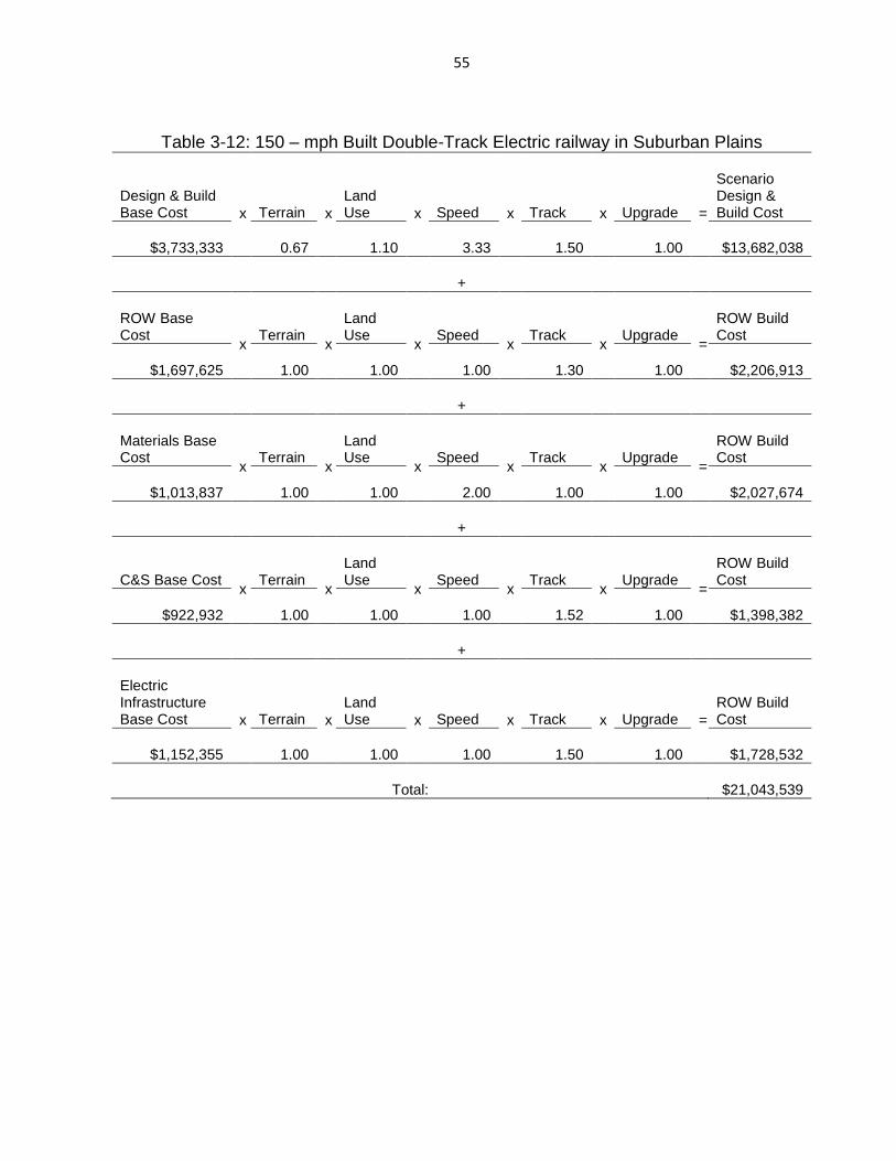
55
Table 3-12: 150 – mph Built Double-Track Electric railway in Suburban Plains
Design & Build Base Cost x Terrain x
Land Use x Speed x Track x Upgrade =
Scenario Design & Build Cost
$3,733,333 0.67 1.10 3.33 1.50 1.00 $13,682,038
+
ROW Base Cost
x Terrain
x
Land Use
x Speed
x Track
x Upgrade
=
ROW Build Cost
$1,697,625 1.00 1.00 1.00 1.30 1.00 $2,206,913
+
Materials Base Cost
x Terrain
x
Land Use
x Speed
x Track
x Upgrade
=
ROW Build Cost
$1,013,837 1.00 1.00 2.00 1.00 1.00 $2,027,674
+
C&S Base Cost x
Terrain x
Land Use
x Speed
x Track
x Upgrade
=
ROW Build Cost
$922,932 1.00 1.00 1.00 1.52 1.00 $1,398,382
+
Electric Infrastructure Base Cost x Terrain x
Land Use x Speed x Track x Upgrade =
ROW Build Cost
$1,152,355 1.00 1.00 1.00 1.50 1.00 $1,728,532
Total: $21,043,539

56
3.6 Methodology Notes
Certain assumptions and limitations of this analysis are worth mentioning.
First, all figures—either components of the methodology or comparative study
costs—have been converted into 2009 dollars (U.S. Army Corps of Engineers,
2000), (Friedman, 2010). Second, the influencing factors are characterized at the
state level, and it is assumed that the costs of a specific project type and for a
certain terrain type will be similar regardless of geographic location. For example,
upgrading a 79mph service to 110mph in a suburban plains location will require the
same types of building requirements regardless of locale, resulting in the same cost.

57
Chapter 4 - CPM Estimation Results
4.1 Results Overview
The CPM methodology (presented in Chapter 3, and summarized in Equation
3-3) was applied for different combinations of influencing factors such as speed, land
use, terrain, and number of tracks. The resulting CPM estimates for building a single
railway track are shown in Table 4-1 The CPM estimates for other speed categories
are available in Appendix A.
Table 4-1: “To Build” Single Track Plains CPM Estimates
Speed Terrain Land Use: Urban Land Use: Suburban Land Use: Rural
79 - mph Non-Electric
Plains
$6,940,911 $4,321,223 $3,495,585
79 - mph Electric $7,534,566 $4,914,877 $4,089,240
110 - mph Non-Electric
$9,146,964 $6,360,436 $5,367,960
110 - mph Electric $9,740,618 $6,954,091 $5,961,614
125 - mph Non-Electric
$13,453,813 $9,843,238 $8,187,633
125 - mph Electric $14,606,168 $10,995,593 $9,339,988
150 - mph Electric $17,866,933 $13,908,108 $11,857,318
220 - mph Electric $25,287,768 $20,476,316 $17,928,161

58
Table 4-2: “To Build” Single Track Hills CPM Estimates
Speed Terrain Land Use: Urban Land Use: Suburban Land Use: Rural
79 - mph Non-Electric
Hills
$8,755,642 $5,774,566 $4,766,946
79 - mph Electric $9,349,296 $6,368,220 $5,360,601
110 - mph Non-Electric
$11,961,227 $8,730,018 $7,472,265
110 - mph Electric $12,554,881 $9,323,672 $8,065,919
125 - mph Non-Electric
$17,578,470 $13,361,274 $11,294,544
125 - mph Electric $18,730,825 $14,513,629 $12,446,899
150 - mph Electric $23,317,484 $18,631,712 $16,044,779
220 - mph Electric $32,730,215 $26,936,527 $23,678,020
Table 4-3: “To Build” Single Track Mountains CPM Estimates
Speed Terrain Land Use: Urban Land Use: Suburban Land Use: Rural
79 - mph Non-Electric
Mountains
$11,641,423 $7,999,545 $6,689,934
79 - mph Electric $12,235,077 $8,593,200 $7,283,589
110 - mph Non-Electric
$16,347,808 $12,330,731 $10,645,919
110 - mph Electric $12,554,881 $9,323,672 $8,065,919
125 - mph Non-Electric
$23,990,894 $18,713,529 $15,977,623
125 - mph Electric $25,143,249 $19,865,884 $17,129,978
150 - mph Electric $31,742,131 $25,808,837 $22,355,989
220 - mph Electric $44,170,112 $36,725,135 $32,330,634

59
Figure 4-1 illustrates the variation of CPM estimates for 220-mph HSR service
by terrain and land use. As planned, the CPM estimates are higher for HSR service
in urban versus suburban and rural areas, as well as on mountainous versus plains
or hills.
Figure 4-1: Summary of “Build” 220-mph Single Track
$0
$5
$10
$15
$20
$25
$30
$35
$40
$45
$50
Plains Hills Mountains
Mill
ion
s
Rural Suburban Urban

60
Figure 4-2, shows similar trends by speed and land use. As it can be
observed, the higher-speed categories reflect considerable increases in cost that are
typically associated with such projects.
Figure 4-2: Double Track CPM Estimates by Service Type
$0
$5
$10
$15
$20
$25
$30
$35
$40
Mill
ion
s
Urban Suburban Rural

61
Figure 4-3 shows that adding new tracks, or upgrading existing tracks, is
more cost-effective than building a new railway. Similar increases in costs as terrain
changes from plains to mountains, and land use from rural to urban are observed.
Note that these trends to apply to a 220-mph HSR service.
Figure 4-3: Example of 220-mph Categorical Cost Changes
The overall pattern of the estimates is as anticipated, where speed, land, and
terrain have a significant effect on CPM estimates. An effort to validate the proposed
CPM methodology and corresponding results is presented in the next Section.
0
10
20
30
40
50
60
70
Additional -Single
Upgrade -Single
Upgrade -Double
Build - Single Build -Double
Mill
ion
s
Rural Plains
Suburban Plains
Urban Plains
Rural Hills
Suburban Hills
Urban Hills
Rural Mountains
Suburban Mountains
Urban Mountains

62
4.2 Validation of the CPM methodology
Validation of the CPM methodology included the following comparisons: 1) a
comparison between existing feasibility study costs per mile and proposed CPM
estimates (“individual comparison”); 2) a comparison between the average cost of all
similar study costs and a range of the proposed CPM estimates (“categorical
comparison”).
4.2.1 Individual CPM Comparison
The individual cost comparison was performed by matching each study cost
with their equivalent CPM cost, according to the proposed methodology. Costs from
feasibility studies, are listed in Table 3-1, and were gathered and converted into
2009 dollars utilizing the CWCCIS index (U.S. Army Corps of Engineers, 2000).
Once the appropriate CPM cost was identified, it was then adjusted to account for
the study cost state influence by a state adjustment factor (U.S. Army Corps of
Engineers, 2000). If a non-location specific study cost was being compared, no
adjustment was made, and if multiple states were involved in the corridor, then an
equally weighted average of the state adjustment factors was utilized.
The study costs were then categorized according to the influencing factors
described in Chapter 3. This included specifying the land use, terrain, speed,
trackage, and motive power for each study cost. In some cases, the characteristics
of the study cost were not clear and the cost amount had to be used as an indicator
of influences, such as number of tracks. The result included 77 study costs over

63
several speed categories from 110 to 220mph, as well as a range of land and terrain
types. A summary of the study costs are available in Table 4-4.
Table 4-4: Summary Statistics of Study Costs (n = 77)
Variables Count Percentage
Track
Single 48 62.3%
Double 29 37.7%
Motive Power
Non-Electric 25 32.5%
Electric 52 67.5%
Construction
Upgrade 26 33.8%
Build 51 66.2%
Additional 0 0.0%
Speed
79mph 0 0.0%
110mph 15 19.5%
125mph 23 29.9%
150mph 12 15.6%
220mph 27 35.1%
Terrain
Plains 72 93.5%
Hills 5 6.5%
Mountains 0 0.0%

64
Table 4-4: Summary Statistics of Study Costs (n = 77) (Continued)
Land Use
Rural 8 10.4%
Suburban 56 72.7%
Urban 13 16.9%
Figure 4-1 shows the comparison of 110 – mph non-electric feasibility study
costs (A-O) and the proposed CPM estimates. The costs include 15 studies
representing 6 different categories. Overall, 60% of the estimates are within +/- 50%
of the study costs. The large discrepancy between study and methodology costs for
“A,” “B,” and “I” could be due to unaccounted regional variability. They are based on
studies in California (A and B) and Florida (I) where population density is likely
higher in the areas most likely to be served, rather than the statewide population
density classification assumed (shown in Figure 3-4).

65
Figure 4-4: Individual Cost Comparison: 110 - mph Non-Electric
Figure 4-5 shows the comparison for 125 – mph non-electric service costs (A-
J). These results represent 10 costs of 3 different categories. The results are
noticeably more accurate, with 80% of the estimates within +/- 50% of the study
costs. Overall, the methodology has been able to replicate the associated study
costs. The outlier, “A,” represents a study cost estimate for a corresponding service
in California.
$0
$1
$2
$3
$4
$5
$6
$7
A B C D E F G H I J K L M N O
Mill
ion
s Study Costs Methodology Costs

66
Figure 4-5: Individual Cost Comparison: 125 - mph Non-Electric
Figure 4-6 shows the comparison for 125 – mph electric service costs (A-M).
These results represent 13 costs of 5 different categories. The results include 46%
of the estimates within +/- 50% of the study costs. The majority of the methodology
cost estimates is higher than the corresponding study costs. Cost “F”, again
represents an under estimation of cost associated with service in California.
$0
$5
$10
$15
$20
$25
A B C D E F G H I J
Mill
ion
s Study Costs Methodology Costs

67
Figure 4-6: Individual Cost Comparison 125 - mph Electric
Figure 4-7 shows the comparison for 150 – mph electric service costs (A-L).
These results represent 12 costs of 4 different categories; with 42% of the
estimations are within +/- 50% of the study costs. As was seen with the 125 – mph
electric comparison, the majority of methodology costs are higher than the study
costs. These overestimations include specific regions, which may indicate incorrect
spatial assumptions including; Texas “A” and “B”, and Chicago “G”-“I” and “K”.
$0
$5
$10
$15
$20
$25
A B C D E F G H I J K L M
Mill
ion
s Study Costs Methodology Costs

68
Figure 4-7: Individual Cost Comparison 150 - mph Electric
Figure 4-8 shows the comparison for 220 – mph electric service costs (A-AA).
These results represent 27 costs of 5 different categories, with 74% of the
estimations within +/- 50% of the study costs. Overall, the methodology and study
costs estimates are close and there are no outlying observations. The highest
difference applies for costs in the Northeast including: New England “I”, Chicago to
the Twin Cities “M” and “N”, Keystone Corridor “O”, and the Empire Corridor “S”.
$0
$5
$10
$15
$20
$25
$30
A B C D E F G H I J K L
Mill
ion
s
Study Costs Methodology Costs

69
Figure 4-8: Individual Cost Comparison 220 - mph Electric
Table 4-5 summarizes the results of the individual cost comparison. 69% of
CPM estimates were within +/- 50% of the study costs.
Table 4-5: Individual Cost Comparison: Statistics (n = 77)
Individual Comparison Count %
Within 10% 15 19%
Within 30% 39 51%
Within 50% 50 69%
Within 80% 63 82%
Over 100% 5 6%
$0
$10
$20
$30
$40
$50
$60
A B C D E F G H I J K L M N O P Q R S T U V W X Y Z AA
Mill
ion
s Study Costs Methodology Costs

70
Upon review of the five individual comparisons, certain trends are evident.
For 110 – mph Non-Electric, 125 - mph Non-Electric, and 125 - mph Electric (Tables
4.4, 4.5, and 4.6), the results show underestimated study costs for California. Upon
review, the likely cause for the undervalued estimation lies with the land use and
terrain classification of the state. Due to the size of the state and location of intended
services (roughly 800 miles from San Diego to Sacramento/San Francisco), all
terrain and land use types are encountered. Therefore the lack of a distinct terrain or
land use influencing factor may require classifying California as multiple geographic
areas rather than one. While not all estimations for California were underestimated
(the 220-mph estimates were within 10% of the study costs), the aforementioned
costs came from the same source, therefore methodological differences may exist
(Federal Railroad Administration, 1997).
Estimations for Texas in the125 - mph Electric and 150 – mph Electric (Figure
4-6 and Figure 4-7) comparisons show similar amounts of overestimation. Upon
review it was determined that the size of Texas may preclude the use of one land
use factor (as shown in Figure 3-5), as a varying mix of all land use types are
encountered between the destination combinations of Dallas/Fort Worth, San
Antonio, and Houston. Other instances of error over 50% were investigated, but no
discernible pattern was determined.
With regards to successful estimation of particular studies or influences, no
overwhelming evidence was found. Possible instances of close estimation of study
costs were identified for two sources, where nearly half of the estimates were within

71
+/- 20% of the study costs ( (Tanaka, et al., 2010), (Parsons Brinckerhoff Quade and
Douglas, Inc., 1991).
Note that true validation may not be possible as the study costs do not
represent completed railway projects, but rather feasibility study estimates. In
addition each project is influenced by local factors (such as Figure 4-4) that may not
be captured in the methodology.
4.2.2 Categorical CPM Comparison
Based on the variability of study costs and the possible error in comparing
average estimates of individual study costs, it was decided to perform a sensitivity
analysis. The sensitivity analysis is intended to better represent a CPM cost, by
taking into account potential variability in the cost components of the methodology.
Table 4-6 shows the contribution of each cost component to the total cost for
two example services (also shown Table 3-11and Table 3-12).

72
Table 4-6: Cost Category Comparison Example
It can be observed that the Design & Build category is found to be the most
influential to the overall cost. As discussed in Section 3.3, the costs associated with
this category was estimated based on four assumptions pertaining to the number of
tracks, terrain, and land multipliers, as well as the build type (upgrade or build)
Of these four assumptions, the land and terrain multipliers were selected as
the most prone to error, as the estimates for material and engineering costs for
upgrades or adding tracks were deemed more realistic. As such, the sensitivity of
the Design & Build cost estimates was examined by changing the terrain multiplier
by +25% (from 1.5 to 1.875 for use when computing hills to mountains, and from
0.667 to 0.833 when computing hills to plains).and -25% (from 1.5 to 1.125 and
0.667 to 0.5, respectively) compared to the base cost. A second test was performed
where the land use multiplier was changed by +25% (from 1.1 to 1.375 for rural to
Cost Component
110 – mph Upgrade Single Non-Electric Suburban Hills
150 – mph Build Double Electric Suburban Plains
Cost % of Total Cost % of Total
Design & Build $2,263,184 71% $13,682,038 65%
Right-of-way $0 0% $2,206,913.12 10%
Materials $508,441 16% $2,027,674 10%
Communications & Signals
$419,390 13% $1,398,382 7%
Electric Infrastructure $0 0% $1,728,532 8%
Total $3,191,014 100% $22,312,871 100%

73
suburban and 1.2 to 1.5 for rural to urban), and -25% (for 1.1 to 0.83 and 1.2 to 0.90,
respectively).
Table 4-7 and Table 4-8 present a summary of the sensitivity analysis results,
that is the lower and upper bounds of CPM estimates, for 150 - mph electric and 220
- mph electric railways respectively. The corresponding results for the other speed
categories are listed in Appendix B (Table C-1, Table C-2, and Table C-3).
Table 4-7: Sensitivity Analysis Results – 150-mph Electric
Terrain Multiplier (+/- 25%) Land Use Multiplier (+/- 25%)
Category Lower Bound
Upper Bound
Difference Lower Bound
Upper Bound
Difference
150 – mph Build Electric Double Suburban Plains
$10,256,400 $17,087,162 $6,830,762 $13,820,240 $17,102,547 $3,282,307
150 – mph Build Electric Double Urban Plains
$11,188,800 $18,640,541 $7,451,741 $14,985,802 $18,657,324 $3,671,522
150 – mph Build Electric Double Rural Plains
$9,324,000 $15,533,784 $6,209,784 $12,438,216 $12,438,216 $0
150 – mph Build Electric Single Suburban Plains
$6,837,600 $11,391,442 $4,553,842 $9,213,493 $11,401,698 $2,188,205
Totals $25,046,129 $9,142,033

74
Table 4-8: Parameter Sensitivity Analysis Comparison – 220-mph Electric
Terrain Multiplier (+/- 25%) Land Use Multiplier (+/- 25%)
Category Lower Bound
Upper Bound
Difference Lower Bound
Upper Bound
Difference
220 – mph Build
Electric Double
Suburban Plains
$18,790,886 $18,790,886 $0 $18,790,886 $18,790,886 $0
220 – mph Build
Electric Double
Urban Hills
$23,253,722 $38,756,203 $15,502,481 $33,959,433 $38,756,203 $4,796,770
220 – mph Build
Electric Double Urban Plains
$20,669,975 $20,669,975 $18,086,228 $22,639,622 $25,837,469 $3,197,847
220 – mph Build
Electric Single
Suburban Plains
$12,527,258 $12,527,258 $0 $12,527,258 $12,527,258 $0
220 – mph Build
Electric Single Urban Plains
$13,779,983 $13,779,983 $0 $15,093,081 $17,224,979 $2,131,898
Totals $33,588,709 $10,126,514

75
The sensitivity analysis results show that the CPM estimates were more
sensitive to the assumptions used to characterize the terrain. Because of this, a
range of CPM estimates is considered instead of a single estimate and is the basis
of the comparison that is discussed next.
4.2.2.1 Categorical Cost Comparison Results
The range of CPM estimates obtained from the sensitivity analysis was
compared against a one-standard deviation range of the average study costs. For a
study bound that is not a range, only one study cost was available, and no range
was calculated. For a methodology bound that is not a range, the category terrain is
the same as the base cost and therefore does not have a multiplier. The results of
this comparison are shown below in Table 4-9.
Table 4-9: Comparison of Categorical CPM Estimates
Label Category Overlap Count
Study Bounds
Methodology Bounds
Overlap
A 220 – mph Build Electric Double
Suburban Plains 14 $18.4 - $33.9 $31.4 Yes
B 220 – mph Build Electric Double Urban
Hills 1 $25.8 $41.2 - $56.7 No
C 220 – mph Build Electric Double Urban
Plains 4 $22.9 - $47.8 $37.9 - $56.0 Yes
D 220 – mph Build Electric Single
Suburban Plains 6 $19.8 - $26.1 $20.5 Yes
E 220 – mph Build Electric Single Urban
Plains 2 $17.6 - $29.3 $25.3 Yes

76
Table 4-10: Comparison of Categorical CPM Estimates (Continued)
Label Category Overlap Count
Study Bounds Methodology Bounds Overlap
F 150 – mph Build Electric Double
Suburban Plains 3 $8.4 - $19.5 $17.6 - $24.4 Yes
G 150 – mph Build Electric Double
Urban Plains 1 $13.9 $22.6 - $30.1 No
H 150 – mph Build Electric Double
Rural Plains 1 $16.2 $15.1 - $21.3 Yes
I 150 - mph Build Electric Single
Suburban Plains 7 $7.3 - $15.0 $11.6 - $16.2 Yes
J 125 – mph Build Electric Double
Suburban Plains 2 $8.1 -$9.4 $14.4 - $19.5 No
K 125 – mph Upgrade Electric
Double Suburban Plains 1 $9.4 $7.6 - $9.3 No
L 125 – mph Upgrade Electric
Double Urban Plains 1 $9.2 $8.8 - $10.6 Yes
M 125 – mph Upgrade Electric
Double Rural Plains 1 $8.80 $7.0 - $8.6 No
N 125 – mph Build Electric Single
Suburban Plains 7 $4.0 - $13.5 $10.0 - $13.4 Yes
O 125 – mph Build Electric Single
Urban Plains 1 $9.30 $12.8 - $16.4 No
P 125 – mph Upgrade Non-
Electric Single Suburban Plains 8 $1.8 - $10.6 $3.7 - $4.8 Yes
Q 125 – mph Upgrade Non-
Electric Single Urban Plains 1 $6.5 $4.6 - $5.8 No
R 125 – mph Build Non-Electric
Single Suburban Plains 1 $5.6 $8.1 - $11.5 No
S 110 – mph Upgrade Non-
Electric Single Suburban Hills 2 $4.8 - $5.4 $3.2 No
T 110 – mph Upgrade Non-
Electric Single Suburban Plains 5 $1.4 - $3.9 $2.0 - $2.8 Yes
U 110 – mph Upgrade Non-
Electric Single Urban Plains 2 $2.3 - $6.1 $2.2 - $3.0 Yes

77
Table 4-10: Comparison of Categorical CPM Estimates (Continued)
Label Category Overlap Count
Study Bounds Methodology Bounds Overlap
V 110 – mph Upgrade Non-Electric Single Rural Hills
2 $1.8 - $3.1 $3.0 Yes
W 110 – mph Upgrade Non-
Electric Single Rural Plains 3 $1.3 $2.0 - $2.6 No
X 110 – mph Build Non-Electric
Single Rural Plains 1 $6.40 $4.0 - $6.1 No
The categorical cost comparison results are more satisfactory than those of
the individual cost comparison, where 54% or 13 out of 24 cost categories overlap,
consisting of 81% of all individual study costs. It should be noted that while there
were some instances of large differences, only 3 of the categories that did not
overlap consisted of more than 1 observation. If all single observation categories
were eliminated, 79% or 11 of 14 cost categories overlap, consisting of 90% of all
individual study costs. While true validation may not be possible for the reasons
mentioned previously, a range of likely costs by cost category seems to be a better
predictor of anticipated construction costs. The CPM estimation methodology can
assist transportation planners in determining preliminary or pre-feasibility study costs
and for project ranking.

78
Chapter 5 – Conclusions, Limitations and Recommendations
5.1 Conclusions
This thesis presented a methodology for estimating the CPM of railway
construction as a function of location and service characteristics such as Figure 4-8.
Five cost components were considered: design and build; ROW; materials; C&S;
and electric infrastructure. A sensitivity analysis was conducted that produced a
range of CPM estimates depending on the assumptions for the influence of terrain
and land use on CPM. While true validation may not be possible as the study costs
do not represent actual railway construction costs but rather feasibility study
estimates, the author conducted the following comparisons: 1) a comparison
between existing feasibility study costs per mile and proposed CPM estimates
(“individual” comparison); 2) a comparison between the average cost of all similar
study costs and a range of the proposed CPM estimates (”categorical comparison”).
It was found that the proposed methodology can predict practical estimates for the
majority of the study costs; over half of the individual study costs can be anticipated
within 50% of their comparable study costs and nearly 80% of the costs by category
being anticipated within the estimated cost ranges. The analysis also showed that
the CPM estimates associated with speed levels (such as Table 4-9) are close to
those estimated in the feasibility studies.
This methodology can be used to produce CPM estimates that are
representative of average values for similar projects at a low cost. It is not meant to
replace the need for feasibility studies, but it is an intermediate tool to help

79
determine the likely project costs based on the service and location of the study
project, and enable further decision by transportation planning professionals. Users
of the CPM methodology can interact with the process in two ways. First, by simply
reviewing the results and second, by interacting with the data to allow revision of the
inputs as more valid and representational information becomes available. It can be
updated with recent information on costs or by including site-specific considerations,
if they are known.
5.2 Limitations and Recommendations
Because of these promising results, continued validation and comparison
may be worthwhile. The limitations of this research as well as recommendations for
future work are discussed below:
Determine if the six base cost sources (New Mexico Rail Runner Express,
California High-Speed-Rail Authority, etc.) are truly representative of railway
construction. For example, utilizing the Florida ROW information (Barton-
Aschman Associates, Inc., et al, 1986) as a representative basis for other areas
may not be as accurate as state or region specific data.
Identify whether the categorization of study costs for comparison has led to an
incorrect classification, where an incorrect interpretation of the source may result
in comparing two dissimilar projects. An example of this may be a study cost that
is not explicit in the number of tracks, resulting in an assumption by the author.

80
Investigate the use of assumptions which were adopted due to the lack of
appropriate information. For example, the use of statewide classifications for
terrain and land use may not accurately represent the actual conditions, as there
might be variations in terrain and land use within a state. Studies not identified or
projects that are completed will help to replace some of these assumptions.
Identify whether the study costs used for comparison are representative of the
technology and location analyzed. This point is of great interest, as each of the
77 costs represents estimates only and no actual project costs. None of these
projects advanced beyond the planning stage. Therefore, it could be assumed
that certain assumptions and calculations were based on parameters that no
longer hold true, and would require reevaluation to be determined representative.
For example, the only HSR project that has been completed during the period
that the studies were published was the upgrading of the New York to Boston
Northeast Corridor segment in 2000 (TGVweb, 2001). Of the studies, 22% were
conducted prior to 1995, 55% were conducted between 1996 and 2000, and the
remaining 23% were conducted between 2009 and 2010. Although all figures
have been escalated into 2009 dollars, adjustments for specific cost inputs, such
as the change in the price of steel were not possible and are almost certainly
worthy of examination when determining the validity of the study data. Future
data collection on detailed CPM figures of completed railway projects is a
promising avenue for validation of this work.
Determine how the range of possible error and its impact might be negated. Each
comparison shows a varying amount of error and determining systematic

81
improvements to limit error may prove unrealistic. By quantifying what is an
acceptable amount of error may help determine the representative nature of the
methodology and its use as a planning tool.
Based on these points, further analysis is recommended to investigate these
potential issues and determine whether the nature of the methodology has been
compromised, or due to lack of completed projects in North America, the results of
the methodology are just as potentially valid as those suggested previously.
Despite these limitations, the CPM estimation methodology shows potential to
allow for pre-feasibility study cost estimation based on characteristics of the service
and location of a project. Increasing demand on the nation’s railroad infrastructure
will necessitate more projects to be carried out that would provide updated
information for potential revisions to the methodology.

82
Appendix A
Right-of-Way cost calculation information as discussed in section 3.3 Cost
Components.
Below is an example of the ROW calculation, including the use of the “Land Use
Type Cost” and multipliers.
Table A-1: ROW Calculation: 79 & 110 – mph Single Track Urban
Land Use Type
Land Use Type Cost Proportion ROW Cost: Single Track
Core $42,905,286
x
3%
= $3,228,906
(Plains) X
1.1 $3,551,797
(Hills) X
1.2 $4,197,578 (Mountains)
Urban $4,291,155 15%
Suburban $3,218,366 32%
Rural $536,394 50%
Land Use Type
Land Use Type Cost Proportion ROW Cost: Double Track
Core $42,905,286
x
3%
X 1.3
$4,197,578 (Plains)
X 1.1
$4,617,336(Hills)
X 1.2
$5,456,851 (Mountains)
Urban $4,291,155 15%
Suburban $3,218,366 32%
Rural $536,394 50%

83
Below are the tables of ROW proportions, for Suburban and Rural.
Table A-2: ROW Proportion Calculations: Urban
Land Use Type
Land Use Type Cost
(2009)
79 - mph, 110 - mph
125 - mph
150 - mph
220 - mph
Urban Urban Urban Urban
Core $42,905,286 3% 5% 5% 5%
Urban $4,291,155 15% 25% 40% 55%
Suburban $3,218,366 32% 30% 25% 30%
Rural $536,394 50% 40% 30% 10%
Table A-3: ROW Proportion Calculations: Suburban
Land Use Type
Land Use Type Cost
Cost Adjusted for
Rural
79 - mph, 110 - mph
125 - mph
150 - mph
220 - mph
Rural Rural Rural Rural
Core $42,905,286
X 0.5 =
$33,791,378 0% 2% 2% 2%
Urban $4,291,155 $3,379,631 10% 20% 30% 30%
Suburban $3,218,366 $2,534,723 30% 25% 33% 53%
Rural $536,394 $422,454 60% 53% 35% 15%

84
Table A-4: ROW Proportion Calculations: Rural
Land Use Type
Land Use Type Cost
Cost Adjusted for
Rural
79 - mph, 110 - mph
125 - mph
150 - mph
220 - mph
Rural Rural Rural Rural
Core $42,905,286
X .25 =
$16,895,689 0% 0% 0% 0%
Urban $4,291,155 $1,689,815 5% 10% 15% 20%
Suburban $3,218,366 $1,267,362 15% 20% 30% 35%
Rural $536,394 $211,227 80% 70% 55% 45%
Below are tables with each ROW cost after the state influence has been removed
Table A-5: ROW Costs: Urban Land Use (Adjusted for state influence)
Terrain Trackage 79 mph, 110 mph 125 mph 150 mph 220 mph
Plains
Single $3,228,906 $4,398,121 $4,827,236 $5,524,549
Double $4,197,578 $5,717,557 $6,275,407 $7,181,913
Hills
Single $3,551,797 $4,837,933 $5,309,960 $6,077,004
Double $4,617,336 $6,289,312 $6,902,947 $7,900,105
Mountains
Single $4,197,578 $5,717,557 $6,275,407 $7,181,913
Double $5,456,851 $7,432,824 $8,158,029 $9,336,487

85
Table A-6: ROW Costs: Suburban Land Use (Adjusted for state influence)
Terrain Trackage 79 mph, 110 mph 125 mph 150 mph 220 mph
Plains
Single $858,231 $1,402,609 $1,697,625 $1,965,823
Double $1,115,700 $1,823,391 $2,206,913 $2,555,569
Hills
Single $944,054 $1,542,869 $1,867,388 $2,162,405
Double $1,227,270 $2,005,730 $2,427,604 $2,811,126
Mountains
Single $1,115,700 $1,823,391 $2,206,913 $2,555,569
Double $1,450,410 $2,370,409 $2,868,987 $3,322,240
Table A-7: ROW Costs: Rural Land Use (Adjusted for state influence)
Terrain Trackage 79 mph, 110 mph 125 mph 150 mph 220 mph
Plains
Single $281,607 $362,066 $476,050 $556,509
Double $366,089 $470,686 $618,865 $723,462
Hills
Single $309,768 $398,273 $523,655 $612,160
Double $402,698 $517,755 $680,751 $795,808
Mountains
Single $366,089 $470,686 $618,865 $723,462
Double $475,916 $611,892 $804,524 $940,500

86
Appendix B
Appendix B contains the Individual CPM Comparisons
Table B-1: CPM to Build Single Track Plains
Speed Terrain Land Use:
Urban Land Use: Suburban
Land Use: Rural
79 - mph Non-Electric
Plains
$6,940,911 $4,321,223 $3,495,585
79 - mph Electric $7,534,566 $4,914,877 $4,089,240
110 - mph Non-Electric
$9,146,964 $6,360,436 $5,367,960
110 - mph Electric $9,740,618 $6,954,091 $5,961,614
125 - mph Non-Electric
$13,453,813 $9,843,238 $8,187,633
125 - mph Electric $14,606,168 $10,995,593 $9,339,988
150 - mph Electric $17,866,933 $13,908,108 $11,857,318
220 - mph Electric $25,287,768 $20,476,316 $17,928,161

87
Table B-2: CPM to Build Single Track Hills
Speed Terrain Land Use:
Urban Land Use: Suburban
Land Use: Rural
79 - mph Non-Electric
Hills
$8,755,642 $5,774,566 $4,766,946
79 - mph Electric $9,349,296 $6,368,220 $5,360,601
110 - mph Non-Electric
$11,961,227 $8,730,018 $7,472,265
110 - mph Electric $12,554,881 $9,323,672 $8,065,919
125 - mph Non-Electric
$17,578,470 $13,361,274 $11,294,544
125 - mph Electric $18,730,825 $14,513,629 $12,446,899
150 - mph Electric $23,317,484 $18,631,712 $16,044,779
220 - mph Electric $32,730,215 $26,936,527 $23,678,020
Table B-3: CPM to Build Single Track Mountains
Speed Terrain Land Use:
Urban Land Use: Suburban
Land Use: Rural
79 - mph Non-Electric
Mountains
$11,641,423 $7,999,545 $6,689,934
79 - mph Electric $12,235,077 $8,593,200 $7,283,589
110 - mph Non-Electric
$16,347,808 $12,330,731 $10,645,919
110 - mph Electric $12,554,881 $9,323,672 $8,065,919
125 - mph Non-Electric
$23,990,894 $18,713,529 $15,977,623
125 - mph Electric $25,143,249 $19,865,884 $17,129,978
150 - mph Electric $31,742,131 $25,808,837 $22,355,989
220 - mph Electric $44,170,112 $36,725,135 $32,330,634

88
Table B-4: CPM to Build Double Track Plains
Speed Terrain Land Use:
Urban Land Use: Suburban
Land Use: Rural
79 - mph Non-Electric
Plains
$9,923,265 $6,467,868 $5,344,737
79 - mph Electric $10,987,972 $7,532,574 $6,409,443
110 - mph Non-Electric
$13,334,337 $9,628,681 $8,255,291
110 - mph Electric $14,399,043 $10,693,387 $9,319,997
125 - mph Non-Electric
$19,691,082 $14,874,322 $12,599,023
125 - mph Electric $21,419,615 $16,602,855 $14,327,555
150 - mph Electric $26,355,855 $21,043,539 $18,211,670
220 - mph Electric $37,942,235 $31,436,802 $27,896,432
Table B-5: CPM to Build Double Track Hills
Speed Terrain Land Use:
Urban Land Use: Suburban
Land Use: Rural
79 - mph Non-Electric
Hills
$12,580,783 $8,630,718 $7,246,145
79 - mph Electric $13,645,490 $9,695,424 $8,310,852
110 - mph Non-Electric
$17,491,154 $13,165,888 $11,406,116
110 - mph Electric $18,555,860 $14,230,595 $12,470,822
125 - mph Non-Electric
$25,790,105 $20,123,323 $17,252,147
125 - mph Electric $27,518,637 $21,851,855 $18,980,680
150 - mph Electric $34,435,136 $28,094,993 $24,483,340
220 - mph Electric $48,995,414 $41,087,802 $36,510,091

89
Table B-6: CPM to Build Double Track Mountains
Speed Terrain Land Use:
Urban Land Use: Suburban
Land Use: Rural
79 - mph Non-Electric
Mountains
$16,780,299 $11,933,858 $10,119,363
79 - mph Electric $17,845,005 $12,998,564 $11,184,070
110 - mph Non-Electric
$23,941,869 $18,532,628 $16,155,334
110 - mph Electric $25,006,576 $19,597,335 $17,220,040
125 - mph Non-Electric
$35,232,816 $28,095,601 $24,262,284
125 - mph Electric $35,157,716 $28,020,501 $24,187,184
150 - mph Electric $46,879,017 $38,792,776 $33,931,113
220 - mph Electric $65,934,278 $55,692,081 $49,466,751
Table B-7: CPM to Build Additional Track Plains
Speed Terrain Land Use:
Urban Land Use: Suburban
Land Use: Rural
79 - mph Non-Electric
Plains
$2,588,965 $1,803,058 $1,555,367
79 - mph Electric $3,182,619 $2,396,713 $2,149,022
110 - mph Non-Electric
$3,393,570 $2,557,612 $2,259,869
110 - mph Electric $3,987,225 $3,151,267 $2,853,524
125 - mph Non-Electric
$5,208,600 $4,125,428 $3,628,746
125 - mph Electric $5,643,797 $5,277,783 $4,222,401
150 - mph Electric $7,522,467 $6,334,819 $5,719,582
220 - mph Electric $11,774,596 $10,331,160 $9,566,714

90
Table B-8: CPM to Build Additional Track Hills
Speed Terrain Land Use:
Urban Land Use: Suburban
Land Use: Rural
79 - mph Non-Electric
Hills
$3,133,384 $2,239,061 $1,936,775
79 - mph Electric $3,727,039 $2,832,716 $2,530,430
110 - mph Non-Electric
$4,237,849 $3,268,486 $2,891,161
110 - mph Electric $4,831,504 $3,862,141 $3,484,815
125 - mph Non-Electric
$6,445,997 $5,180,838 $2,891,161
125 - mph Electric $7,598,352 $6,333,193 $5,713,174
150 - mph Electric $9,157,632 $7,751,901 $6,975,821
220 - mph Electric $14,007,330 $12,269,224 $11,291,671
Table B-9: CPM to Build Additional Track Mountains
Speed Terrain Land Use:
Urban Land Use: Suburban
Land Use: Rural
79 - mph Non-Electric
Mountains
$3,999,118 $2,906,555 $2,513,672
79 - mph Electric $4,592,773 $3,500,210 $3,107,326
110 - mph Non-Electric
$5,553,824 $4,348,700 $3,843,257
110 - mph Electric $6,147,478 $4,942,355 $4,436,912
125 - mph Non-Electric
$8,369,724 $6,786,515 $3,843,257
125 - mph Electric $9,522,079 $7,938,870 $7,118,098
150 - mph Electric $11,685,026 $9,905,038 $8,869,184
220 - mph Electric $17,439,299 $15,205,806 $13,887,456

91
Table B-10: CPM to Upgrade Single Track Plains
Speed Terrain Land Use:
Urban Land Use: Suburban
Land Use: Rural
79 - mph Non-Electric
Plains
$1,709,938 $1,627,763 $1,241,134
79 - mph Electric $2,303,592 $2,221,418 $2,139,244
110 - mph Non-Electric
$2,574,605 $2,437,374 $2,300,143
110 - mph Electric $3,168,260 $3,031,029 $2,893,797
125 - mph Non-Electric
$5,210,117 $4,258,268 $3,795,162
125 - mph Electric $6,362,472 $5,410,623 $4,947,517
150 - mph Electric $7,579,622 $6,523,579 $5,944,544
220 - mph Electric $11,911,768 $10,608,687 $9,880,541
Table B-11: CPM to Upgrade Single Track Hills
Speed Terrain Land Use:
Urban Land Use: Suburban
Land Use: Rural
79 - mph Non-Electric
Hills
$3,090,194 $2,315,059 $2,033,287
79 - mph Electric $3,683,849 $2,908,713 $2,626,941
110 - mph Non-Electric
$4,284,707 $3,427,028 $3,062,712
110 - mph Electric $4,878,362 $4,020,682 $3,656,367
125 - mph Non-Electric
$6,536,069 $5,407,999 $4,817,546
125 - mph Electric $7,688,424 $6,560,354 $5,969,901
150 - mph Electric $9,339,686 $8,068,787 $7,322,598
220 - mph Electric $14,323,579 $12,724,830 $11,773,542

92
Table B-12: CPM to Upgrade Single Track Mountains
Speed Terrain Land Use:
Urban Land Use: Suburban
Land Use: Rural
79 - mph Non-Electric
Mountains
$3,990,840 $3,035,570 $2,663,367
79 - mph Electric $3,990,840 $3,035,570 $2,663,367
110 - mph Non-Electric
$5,680,617 $4,601,531 $4,105,513
110 - mph Electric $5,680,617 $4,601,531 $4,105,513
125 - mph Non-Electric
$8,581,799 $7,151,801 $6,357,169
125 - mph Electric $8,581,799 $7,151,801 $6,357,169
150 - mph Electric $12,042,584 $10,410,076 $9,397,680
220 - mph Electric $18,010,352 $15,923,617 $14,620,001
Table B-13: CPM to Upgrade Double Track Plains
Speed Terrain Land Use:
Urban Land Use: Suburban
Land Use: Rural
79 - mph Non-Electric
Plains
$2,722,587 $2,599,325 $2,476,063
79 - mph Electric $3,787,293 $3,664,031 $2,460,807
110 - mph Non-Electric
$4,121,580 $3,915,733 $3,709,887
110 - mph Electric $4,715,235 $4,509,388 $4,774,593
125 - mph Non-Electric
$7,985,256 $6,707,258 $6,064,626
125 - mph Electric $9,137,611 $7,859,613 $7,793,158
150 - mph Electric $11,648,974 $10,221,389 $9,413,916
220 - mph Electric $18,706,917 $16,930,231 $15,908,478

93
Table B-14: CPM to Upgrade Double Track Hills
Speed Terrain Land Use:
Urban Land Use: Suburban
Land Use: Rural
79 - mph Non-Electric
Hills
$4,615,381 $3,583,065 $3,192,122
79 - mph Electric $5,680,088 $4,647,771 $3,785,776
110 - mph Non-Electric
$6,509,144 $5,353,011 $4,838,252
110 - mph Electric $7,102,798 $5,946,666 $5,902,959
125 - mph Non-Electric
$9,809,254 $8,379,256 $7,596,391
125 - mph Electric $11,104,548 $9,577,196 $9,324,924
150 - mph Electric $14,264,933 $12,530,714 $11,478,616
220 - mph Electric $22,297,010 $20,094,617 $18,745,197
Table B-15: CPM to Upgrade Double Track Mountains
Speed Terrain Land Use:
Urban Land Use: Suburban
Land Use: Rural
79 - mph Non-Electric
Mountains
$5,934,060 $4,655,250 $4,134,426
79 - mph Electric $6,998,767 $5,719,956 $4,728,081
110 - mph Non-Electric
$8,570,719 $7,106,184 $6,399,637
110 - mph Electric $9,164,373 $7,699,839 $7,464,343
125 - mph Non-Electric
$12,690,929 $10,935,349 $9,902,206
125 - mph Electric $14,129,161 $12,178,874 $11,630,738
150 - mph Electric $18,271,008 $16,025,671 $14,586,480
220 - mph Electric $27,771,925 $24,873,140 $23,009,320

94
Appendix C
Appendix C includes the remainder of the speed category specific parameter sensitivity
analysis from Chapter 5.
Table C-1: Parameter Sensitivity Analysis Comparison – 110-mph
Category
Terrain Method Lower Bound
Terrain Method Upper Bound
Terrain Diff
Land Use Method Lower Bound
Land Use Method Upper Bound
Land Use Diff
Upgrade Non-Electric
Single Suburban
Hills
$2,263,184 $2,263,184 $0 $2,286,044 $2,828,980 $542,936
Upgrade Non-Electric
Single Suburban
Plains
$1,131,592 $1,885,232 $753,640 $1,524,792 $1,886,930 $362,138
Upgrade Non-Electric
Single Urban Plains
$1,234,464 $2,056,617 $822,153 $1,653,389 $2,058,469 $405,080
Upgrade Non-Electric Single Rural
Hills
$2,057,440 $2,057,440 $0 $2,057,440 $2,057,440 $0
Upgrade Non-Electric Single Rural
Plains
$1,028,720 $1,713,848 $685,128 $1,372,312 $1,372,312 $0
Build Non-Electric
Single Rural Plains
$3,117,333 $5,193,477 $2,076,144 $4,158,523 $4,158,523 $0
Totals $4,337,065 $1,310,154

95
Table C-2: Parameter Sensitivity Analysis Comparison – 125-mph
Category
Terrain Method Lower Bound
Terrain Method Upper Bound
Terrain Diff
Land Use Method Lower Bound
Land Use Method Upper Bound
Land Use Diff
Upgrade Non-Electric Single
Suburban Plains
$1,673,672 $2,788,338 $1,114,666 $2,255,231 $2,790,848 $535,617
Upgrade Non-Electric Single Urban Plains
$1,825,824 $3,041,823 $1,215,999 $2,445,431 $3,044,562 $599,131
Build Non-Electric Single
Suburban Plains
$5,071,733 $5,071,733 $0 $6,834,033 $8,457,115 $1,623,083
Totals $2,330,664 $2,757,831

96
Table C-3: Parameter Sensitivity Analysis Comparison – 125-mph Electric
Category
Terrain Method Lower Bound
Terrain Method Upper Bound
Terrain Diff
Land Use Method Lower Bound
Land Use Method
Upper Bound
Land Use Diff
Build Electric Double
Suburban Plains
$7,607,600 $12,674,262 $5,066,662 $10,251,049 $12,685,673 $2,434,624
Upgrade Electric Double
Suburban Plains
$2,510,508 $4,182,506 $1,671,998 $3,382,846 $4,186,272 $803,426
Upgrade Electric
Double Urban Plains
$2,738,736 $4,562,734 $1,823,998 $3,668,146 $4,566,842 $898,696
Upgrade Electric
Double Rural Plains
$2,282,280 $3,802,278 $1,519,998 $3,044,562 $3,044,562 $0
Build Electric Single
Suburban Plains
$5,071,733 $8,449,508 $3,377,774 $6,834,033 $8,457,115 $1,623,083
Build Electric Single Urban
Plains $5,532,800 $9,217,645 $3,684,845 $7,410,397 $9,225,944 $1,815,547
Totals $17,145,276 $7,575,376

97
Table C-4: Parameter Sensitivity Analysis Comparison – 150-mph Electric
Category
Terrain Method Lower Bound
Terrain Method Upper Bound
Terrain Diff
Land Use Method Lower Bound
Land Use Method Upper Bound
Land Use Diff
Build Electric Double
Suburban Plains
$10,256,400 $17,087,162 $6,830,762 $13,820,240 $17,102,547 $3,282,307
150 – mph Build Electric
Double Urban Plains
$11,188,800 $18,640,541 $7,451,741 $14,985,802 $18,657,324 $3,671,522
Build Electric Double Rural
Plains $9,324,000 $15,533,784 $6,209,784 $12,438,216 $12,438,216 $0
Build Electric Single
Suburban Plains
$6,837,600 $11,391,442 $4,553,842 $9,213,493 $11,401,698 $2,188,205
Totals $25,046,129 $9,142,033

98
Table C-5: Parameter Sensitivity Analysis Comparison – 220-mph Electric
Category
Terrain Method Lower Bound
Terrain Method Upper Bound
Terrain Diff
Land Use Method Lower Bound
Land Use Method Upper Bound
Land Use Diff
Build Electric Double
Suburban Plains
$18,790,886 $18,790,886 $0 $18,790,886 $18,790,886 $0
Build Electric Double
Urban Hills $23,253,722 $38,756,203 $15,502,481 $33,959,433 $38,756,203 $4,796,770
220 –mph Build Electric
Double Urban Plains
$20,669,975 $20,669,975 $0 $22,639,622 $25,837,469 $3,197,847
Build Electric Single
Suburban Plains
$12,527,258 $12,527,258 $0 $12,527,258 $12,527,258 $0
Build Electric Single Urban
Plains $13,779,983 $13,779,983 $0 $15,093,081 $17,224,979 $2,131,898
Totals $15,502,481 $10,126,514

99
Appendix D
Individual cost comparisons as referred to in Chapter 5.
Figure D-1: Individual Cost Comparison 110 - mph Non-Electric – Graph
Table D-1: Individual Cost Comparison Statistics: 110 - mph Non-Electric
Individual Cost Comparison Statistics: 110 - mph Non-Electric
Individual Comparison Count %
Within 10% 3 20%
Within 30% 5 33%
Within 50% 9 60%
Within 80% 13 87%
Over 100% 0 0%
$0
$1
$2
$3
$4
$5
$6
$7
A B C D E F G H I J K L M N O
Mill
ion
s
Study Costs Methodology Costs

100
Table D-2: Individual Cost Comparison 110 - mph Non-Electric Data
State Code Category Study Costs
Methodology Costs
Difference $ Difference
%
California North & South
A Upgrade Single
Non-Electric Suburban Hills
$6,256,335 $2,876,101 -$3,380,233 -54.0%
California South
B Upgrade Single
Non-Electric Suburban Hills
$5,785,953 $2,876,101 -$2,909,852 -50.3%
Chicago Hub
C Upgrade Single
Non-Electric Suburban Plains
$2,235,358 $3,425,022 $1,189,664 53.2%
Chicago to Detroit
D Upgrade Single
Non-Electric Suburban Plains
$2,441,762 $3,393,112 $951,350 39.0%
Chicago to St. Louis
E Upgrade Single
Non-Electric Suburban Plains
$2,435,601 $3,637,756 $1,202,155 49.4%
Charlotte to Macon
F Upgrade Single
Non-Electric Suburban Plains
$4,114,790 $2,733,636 -$1,381,155 -33.6%
PBD&Q Suburban
G Upgrade Single
Non-Electric Suburban Plains
$1,731,007 $3,191,014 $1,460,008 84.3%
PBD&Q Urban
H Upgrade Single
Non-Electric Urban Plains
$2,844,483 $2,574,605 -$269,878 -9.5%
Florida I Upgrade Single
Non-Electric Urban Plains
$5,226,155 $2,420,129 -$2,806,026 -53.7%
Pacific Northwest
J Upgrade Single
Non-Electric Rural Hills
$2,162,814 $3,194,239 $1,031,425 47.7%
Texas Triangle
K Upgrade Single
Non-Electric Rural Hills
$2,511,828 $2,597,185 $85,357 3.4%
PBD&Q Rural
L Upgrade Single
Non-Electric Rural Plains
$1,270,784 $2,300,143 $1,029,358 81.0%

101
Table D-2: Individual Cost Comparison 110 – mph Non-Electric Data (Continued)
State Code Category Study Costs
Methodology Costs
Difference $ Difference
%
Chicago to Twin Cities
M Upgrade Single
Non-Electric Rural Plains
$2,551,755 $2,300,143 -$251,612 -9.9%
Chicago to Twin Cities
N Upgrade Single
Non-Electric Rural Plains
$3,162,180 $2,300,143 -$862,037 -27.3%
Chicago to Twin Cities
O Build Single Non-
Electric Rural Plains
$6,415,385 $5,086,353 -$1,329,032 -20.7%

102
Figure D-2: Individual Cost Comparison 125 - mph Non-Electric - Graph
Table D-3: Individual Cost Comparison Statistics: 125 - mph Non-Electric
Individual Cost Comparison Statistics: 125 - mph Non-Electric
Individual Comparison Count %
Within 10% 3 30%
Within 30% 6 60%
Within 50% 8 80%
Within 80% 10 100%
Over 100% 0 0%
$0
$5
$10
$15
$20
$25
A B C D E F G H I J
Mill
ion
s Study Costs Methodology Costs

103
Table D-4: Individual Cost Comparison: 125 - mph Non-Electric - Data
State Code Category Study Costs Methodology
Costs Difference $
Difference %
California North & South
A Upgrade Single
Non-Electric Suburban Plains
$19,789,565 $5,024,756 -$14,764,809 -74.6%
California South
B Upgrade Single
Non-Electric Suburban Plains
$6,206,708 $5,024,756 -$1,181,951 -19.0%
Chicago Hub
C Upgrade Single
Non-Electric Suburban Plains
$4,380,619 $4,570,541 $189,922 4.3%
Chicago to Detroit
D Upgrade Single
Non-Electric Suburban Plains
$4,713,486 $4,527,958 -$185,527 -3.9%
Chicago to St. Louis
E Upgrade Single
Non-Electric Suburban Plains
$4,476,983 $4,854,426 $377,443 8.4%
Pacific Northwest
F Upgrade Single
Non-Electric Suburban Plains
$3,316,608 $4,556,347 $1,239,739 37.4%
Texas Triangle
G Upgrade Single
Non-Electric Suburban Plains
$6,316,832 $3,704,693 -$2,612,139 -41.4%
Ontario to Quebec
H Upgrade Single
Non-Electric Suburban Plains
$5,005,903 $4,407,307 -$598,596 -12.0%
Florida I Upgrade Single
Non-Electric Urban Plains
$6,122,007 $4,897,510 -$1,224,497 -20.0%
Charlotte to Macon
J Build Single Non-Electric
Suburban Plains $4,795,920 $7,230,806 $2,434,886 50.8%

104
Figure D-3: Individual Cost Comparison 125 - mph Electric – Graph
Table D-5: Individual Cost Comparison Statistics: 125 - mph Electric
Individual Cost Comparison Statistics: 125 - mph Electric
Individual Comparison Count %
Within 10% 0 0%
Within 30% 4 31%
Within 50% 6 46%
Within 80% 8 62%
Over 100% 3 23%
$0
$5
$10
$15
$20
$25
A B C D E F G H I J K L M
Mill
ion
s
Study Costs Methodology Costs

105
Table D-6: Individual Cost Comparison: 125 - mph Electric - Data
State Code Category Study Costs Methodology
Costs Difference $
Difference %
Texas A Build Double
Electric Suburban Plains
$7,235,145 $14,778,148 $7,543,003 104.3%
Texas B Build Double
Electric Suburban Plains
$8,007,451 $14,778,148 $6,770,696 84.6%
PBD&Q Suburban
C Upgrade Double
Electric Suburban Plains
$10,775,756 $8,435,790 -$2,339,966 -21.7%
PBD&Q Urban
D Upgrade Double Electric Urban
Plains $13,117,102 $9,713,788 -$3,403,314 -25.9%
PBD&Q Rural
E Upgrade Double
Electric Rural Plains
$8,756,425 $7,793,158 -$963,267 -11.0%
California North & South
F Build Single
Electric Suburban Plains
$22,640,247 $13,862,166 -$8,778,081 -38.8%
California South
G Build Single
Electric Suburban Plains
$9,314,573 $13,862,166 $4,547,593 48.8%
Chicago Hub
H Build Single
Electric Suburban Plains
$6,988,238 $12,609,089 $5,620,851 80.4%
Chicago to Detroit
I Build Single
Electric Suburban Plains
$7,640,361 $12,491,613 $4,851,252 63.5%
Chicago to St. Louis
J Build Single
Electric Suburban Plains
$6,636,731 $13,392,262 $6,755,531 101.8%
Pacific Northwest
K Build Single
Electric Suburban Plains
$5,924,977 $12,569,930 $6,644,953 112.2%
Texas Triangle
L Build Single
Electric Suburban Plains
$7,885,553 $10,220,411 $2,334,858 29.6%

106
Table D-6: Individual Cost Comparison: 125 - mph Electric – Data (Continued)
State Code Category Study Costs Methodology
Costs Difference $
Difference %
Florida M Build Single
Electric Urban Plains
$8,720,606 $13,729,798 $5,009,192 57.4%

107
Figure D-4: Individual Cost Comparison 150 - mph Electric – Graph
Table D-7: Individual Cost Comparison Statistics: 150 - mph Electric
Individual Cost Comparison Statistics: 150 - mph Electric
Individual Comparison Count %
Within 10% 1 8%
Within 30% 4 33%
Within 50% 5 42%
Within 80% 8 67%
Over 100% 2 17%
$0
$5
$10
$15
$20
$25
$30
A B C D E F G H I J K L
Mill
ion
s
Study Costs Methodology Costs

108
Table D-8: Individual Cost Comparison: 150 - mph Electric - Data
State Code Category Study Costs
Methodology Costs
Difference $ Difference
%
Texas A Build Double
Electric Suburban Plains
$8,946,569 $18,307,879 $9,361,311 104.6%
Texas B Build Double
Electric Suburban Plains
$9,817,171 $18,307,879 $8,490,708 86.5%
PBD&Q Suburban.
C Build Double
Electric Suburban Plains
$20,358,762
$21,043,539 $684,777 3.4%
PBD&Q Urban
D Build Double
Electric Urban Plains
$13,910,456
$26,355,855 $12,445,399 89.5%
PBD&Q Rural
E Build Double Electric Rural
Plains
$16,241,354
$18,211,670 $1,970,316 12.1%
California North & South
F Build Single
Electric Suburban Plains
$23,085,266
$16,411,568 -$6,673,698 -28.9%
Chicago Hub
G Build Single
Electric Suburban Plains
$10,231,867
$14,928,036 $4,696,169 45.9%
Chicago to Detroit
H Build Single
Electric Suburban Plains
$8,750,222 $14,788,955 $6,038,733 69.0%
Chicago to St. Louis
I Build Single
Electric Suburban Plains
$12,013,032
$15,855,243 $3,842,211 32.0%
Texas Triangle
J Build Single
Electric Suburban Plains
$10,047,430
$12,100,054 $2,052,624 20.4%
Chicago to Twin Cities
K Build Single
Electric Suburban Plains
$10,550,137
$15,623,441 $5,073,305 48.1%
Charlotte to Macon
L Build Single
Electric Suburban Plains
$7,919,904 $11,914,613 $3,994,709 50.4%

109
Figure D-5: Individual Cost Comparison 220 - mph Electric – Graph
Table D-9: Individual Cost Comparison Statistics: 220 - mph Electric
Individual Cost Comparison Statistics: 220 - mph Electric
Individual Comparison Count %
Within 10% 9 33%
Within 30% 19 70%
Within 50% 20 74%
Within 80% 21 78%
Over 100% 5 19%
$0
$10
$20
$30
$40
$50
$60
A B C D E F G H I J K L M N O P Q R S T U V W X Y Z AA
Mill
ion
s Study Costs Methodology Costs

110
Table D-10: Individual Cost Comparison: 220 - mph Electric – Data
State Code Category Study Costs Methodology
Costs Difference $
Difference %
California North & South
A Build Double
Electric Suburban Plains
$39,190,694 $37,095,427 -$2,095,268 -5.3%
California South
B Build Double
Electric Suburban Plains
$39,981,039 $37,095,427 -$2,885,613 -7.2%
California C Build Double
Electric Suburban Plains
$44,133,968 $37,095,427 -$7,038,541 -15.9%
Pacific Northwest
D Build Double
Electric Suburban Plains
$16,974,603 $33,637,378 $16,662,775 98.2%
Chicago Hub
E Build Double
Electric Suburban Plains
$28,129,342 $33,742,168 $5,612,826 20.0%
South Central
F Build Double
Electric Suburban Plains
$27,159,365 $27,507,202 $347,837 1.3%
South East G Build Double
Electric Suburban Plains
$23,279,456 $27,585,794 $4,306,338 18.5%
Gulf H Build Double
Electric Suburban Plains
$23,279,456 $28,057,346 $4,777,890 20.5%
New England
I Build Double
Electric Suburban Plains
$22,794,467 $35,314,008 $12,519,541 54.9%
Texas J Build Double
Electric Suburban Plains
$23,419,120 $27,350,018 $3,930,898 16.8%
Texas K Build Double
Electric Suburban Plains
$23,304,481 $27,350,018 $4,045,537 17.4%
Chicago to St. Louis
L Build Double
Electric Suburban Plains
$39,115,868 $35,837,955 -$3,277,913 -8.4%

111
Table D-10: Individual Cost Comparison: 220 - mph Electric – Data (Continued)
State Code Category Study Costs Methodology
Costs Difference $
Difference %
Chicago to Twin Cities
M Build Double
Electric Suburban Plains
$12,888,199 $35,314,008 $22,425,809 174.0%
Chicago to Twin Cities
N Build Double
Electric Suburban Plains
$18,447,205 $35,314,008 $16,866,803 91.4%
Keystone Corridor
O Build Double
Electric Urban Hills $28,129,342 $53,405,001 $25,275,659 89.9%
Northeast Corridor
P Build Double
Electric Urban Plains
$56,677,920 $43,017,009 -$13,660,912 -24.1%
Florida Q Build Double
Electric Urban Plains
$34,434,195 $35,665,701 $1,231,506 3.6%
Northeast Corridor
R Build Double
Electric Urban Plains
$39,769,070 $43,017,009 $3,247,939 8.2%
Empire Corridor
S Build Double
Electric Urban Plains
$22,794,467 $44,012,992 $21,218,525 93.1%
Chicago Hub
T Build Single Electric
Suburban Plains $27,604,848 $21,977,913 -$5,626,935 -20.4%
Chicago to Detroit
U Build Single Electric
Suburban Plains $25,385,207 $21,773,150 -$3,612,058 -14.2%
Chicago to St. Louis
V Build Single Electric
Suburban Plains $27,331,015 $23,343,001 -$3,988,014 -14.6%
Pacific Northwest
W Build Single Electric
Suburban Plains $24,046,957 $21,909,659 -$2,137,299 -8.9%
Texas Triangle
X Build Single Electric
Suburban Plains $14,670,938 $17,814,395 $3,143,458 21.4%
Southeast Y Build Single Electric
Suburban Plains $21,701,542 $17,967,968 -$3,733,575 -17.2%

112
Table D-10: Individual Cost Comparison: 220 - mph Electric – Data (Continued)
State Code Category Study Costs Methodology
Costs Difference $
Difference %
Florida Z Build Single Electric
Urban Plains $18,159,755 $23,770,502 $5,610,747 30.9%
Empire Corridor
AA Build Single Electric
Urban Plains $32,029,067 $29,333,811 -$2,695,256 -8.4%

113
Bibliography
Administration, Federal Highway. 2011. High-Speed Intercity Passenger Rail Program, Federal
Investment Highlights (2009-11). Federal Highway Administration, Washington DC : 2011.
American Railway Engineering and Maintenance of Way Association. 2003. Practical Guide to
Railway Engineering, Second Edition. Landover, MD : American Railway Engineering and
Maintenance of Way Association, 2003.
Amtrak. 2010. A Vision for Hish-Speed Rail in the Northeast Corridor. Washington DC : Amtrak, 2010.
Armstrong, John H. 2008. The Railroad What It Is, What It Does, 5th Edition. Omaha, NE : Simmons-
Boardman Books, Inc., 2008. 978-0-911382-58-7.
Association of American Railroads. 2010. Class I Railroad Statistics. Association of American
Railroads. [Online] October 29, 2010. [Cited: December 13, 2010.]
http://aar.org/~/media/aar/Industry%20Info/AAR%20Stats%202010%201123.ashx.
—. Positive Train Control. Association of American Railroads. [Online] [Cited: December 13, 2010.]
http://www.aar.org/~/media/aar/backgroundpapers/positivetraincontrol.ashx.
Barton-Aschman Associates, Inc., Robert J. Harmon Associates, Inc., Metric Engineering, and
Bachman Associates. 1986. Florida High Speed Rail Study. s.l. : BAAI, 1986.
Buczynski, Beth. 2010. Amtrak Spends $466 Million on Electric Locomotives. Earth & Industry.
[Online] October 30, 2010. [Cited: August 5, 2011.] http://earthandindustry.com/2010/10/amtrak-
spends-466-million-on-electric-locomotives/.
California High-Speed Rail Authority. 2009. Business Plan, "Report to the Legislature, December
2009". California High-Speed Rail Authority. [Online] December 2009.
http://www.cahighspeedrail.ca.gov/Business_Plan_reports.aspx.
Cambridge Systematics. 2005. Transportation Invest in America: Freight-Rail Bottom Line Report.
Cambridge, MA : Cambridge Systematics, 2005.
Cambridge Systematics, Inc. 2007. National Rail Freight Infrastructure Capacity and Investment
Study. Washington DC : Association of American Railroads, 2007.
CBO. 2006. Freight Rail Transportation: Long-Term Issues. Washington D.C. : Congressional Budget
Office CBO, 2006.
Cox, Wendell, Vranich, Joseph and Moore, Adrian T. 2008. The California High Speed Rail Proposal:
A Due Diligence Report. s.l. : Reason Foundation, 2008.

114
de Cerreno, Allison L.C. and Mathur, Shishir. 1991. High-Speed Rail Projects in the United States:
Identifying The Elements of Success Part 2. San Jose, CA : Mineta Transportation Institute, 1991.
ESRI Press. 2008. GIS Tutorial Exercise Data, Workbook for Arc View 9, Third Edition. 2008.
Federal Railroad Administration. 2007. Electronically Controlled pneumatic Brake Systems. Federal
Register, the Daily Journal of the United States Government. [Online] September 4, 2007. [Cited:
December 13, 2010.] http://www.federalregister.gov/articles/2007/09/04/07-4297/electronically-
controlled-pneumatic-brake-systems#p-250.
—. 1997. High-Speed Ground Transportation For America, Statistical Supplement. Washington DC :
US Department of Transportation, 1997.
—. 2011. High-Speed Intercity Passenger Rail Program. Federal Railroad Administration. [Online]
August 5, 2011. http://www.fra.dot.gov/rpd/passenger/2243.shtml.
—. 2010. Impact of the Staggers Rail Act of 1980. United States Department of Transportation,
Federal Railroad Administration. [Online] December 13, 2010.
http://www.fra.dot.gov/downloads/policy/staggers_rail_act_impact.pdf.
—. 2011. Northeast Corridor Main Line. Federal Railroad Administration. [Online] 2011. [Cited: June
1, 2011.] http://www.fra.dot.gov/rpd/passenger/643.shtml.
—. Positive Train Control (PTC). United States Department of Transportation. [Online] [Cited: August
8, 2011.] http://www.fra.dot.gov/Pages/784.shtml.
—. 2011. Vision for High-Speed Rail in America. Federal Railroad Administration. [Online] March 15,
2011. [Cited: June 10, 2011.] http://www.fra.dot.gov/rpd/downloads/HSR_Map_2011_03_15.pdf.
Friedman, S. Morgan. 2010. The Inflation Calculator. [Online] 2010. [Cited: February 8, 2010.]
http://www.westegg.com/inflation/.
General Electric. PowerHaul Series Locomotive. GE Transportation. [Online] [Cited: August 5, 2011.]
http://www.getransportation.com/rail/rail-products/locomotives/powerhaul-series-
locomotive.html.
Hagler, Yoav and Todorovish, Petra. 2009. Where High-Speed Rail Works Best. New York City :
America 2050, 2009.
Illinois Department of Transportation. 2011. Official IDOT Fact Sheet. Illinois Department of
Transportation High Speed Rail. [Online] 2011. [Cited: June 18, 2011.]
http://www.idothsr.org/pdf/fact%20sheet%20-%20february%202011.pdf.

115
Lindahl, Martin. 2001. Track geometry for high-speed railways, A literature survey and simulation of
dynamic vehicle response. Stockholm, Sweden : Railway Technology, Department of Vehicle
Engineering, Royal Institute of Technology., 2001. 1103-470X.
Mandelbaum, Robb. 2009. Stop That Train! ieee Spectrum Inside Technology. [Online] March 2009.
[Cited: August 8, 2011.] http://spectrum.ieee.org/green-tech/mass-transit/stop-that-train.
Mid Region Council of Governments, New Mexico Department of Transportation. 2008. Belen to
Santa Fe Commuter Rail Project Overview and Status of Project Elements. New Mexico Rail Runner
Express. [Online] October 8, 2008. [Cited: February 20, 2010.]
http://nmrailrunner.com/STATUS/LFCBelen%20to%20Santa%20Fe%20Update100808.doc.
Midwest High Speed Rail Association. 2011. Illinois. Midwest High Speed Rail Association,
Transforming the Midwest by Transforming Travel. [Online] 2011. [Cited: June 18, 2011.]
http://www.midwesthsr.org/projects-illinois.
Murray, Tom. 2006. Investing in railroads. Trains: The magazine of railroading. [Online] July 7, 2006.
[Cited: December 13, 2010.]
http://trn.trains.com/en/Railroad%20Reference/Freight%20Railroads/2006/07/Investing%20in%20r
ailroads.aspx.
Nash, Andrew. 2003. Best Practices in Shared-Use High-Speed Rail Systems . San Jose, CA : Mineta
Transportation Institute , 2003.
Ontario / Québec Rapid Train Task Force. 1991. Ontario / Québec Rapid Train Task Force Final
Report. www.bv.transports.gouv.qc.ca. [Online] 1991. [Cited: October 6, 2011.]
http://www.bv.transports.gouv.qc.ca/mono/0986299.pdf.
Parsons Brinckerhoff Quade and Douglas, Inc. 1991. Cost and Travel Time Estimation for a
Hypothetical Corridor. [book auth.] Transportation Research Board. Special Report 233, In Pursuit of
Speed: New Options for Intercity Passenger Transport. Washington D.C. : Transportation Research
Board, National Research Council, 1991.
Peterman, David Randall, Frittelli, John and Mallett, William J. 2009. High Speed Rail (HSR) in the
United States. Washington DC : Congressional Research Service, 2009.
Saunders Jr., Richard. 2003. Main Lines: Rebirth of the North American Railroads, 1970-2002.
Dekalb, IL : Northen Illinois University Press, 2003.
Schwarm, Edward G. and Little, Arthur D. 1977. Capital and Maintenance Costs for Fixed Railroad
Electrification Facilities. [book auth.] Transportation Research Board. Railroad Electrification: The
Issues. Washington D.C. : s.n., 1977, pp. 42-47.

116
Speeding up commuter rail service: comparative actual performance of different train and station
platform designs. Morlok, Edward K. and Nitzberg, Bradley F. 2004. Washington DC :
Transportation Research Board, 2004.
SunRail. 2011. What is commuter rail? SunRail. [Online] 2011. [Cited: September 29, 2011.]
http://www.cfrail.com/cr_whatiscommuterrail.asp.
Tanaka, Yuki, et al. 2010. Analysis of High-Speed Rail's Potential To Reduce CO2 Emissions From
Transportation in the United States. Lisbon, Portugal : World Conference on Transport Research,
2010.
Texas Turnpike Authority, Lichliter/Jameson & Associates, Inc, Wilbur Smith Associates, Inc,
Morrison-Knudsen, M.Ray Perryman Consultants, Inc, Underwood, Neuhaus & Co. Incorporated,
Sylva Engineering Corportation, Andrews & Kurth. 1989. Texas Triangle High Speed Rail Study.
Austin, TX : Texas Turnpike Authority, 1989.
TGVweb. 2001. Acela Express. TGVweb. [Online] February 2001. [Cited: June 12, 2011.]
http://www.trainweb.org/tgvpages/acela.html#dates.
—. 1998. The TGV Signaling System. TGVweb. [Online] April 23, 1998. [Cited: June 27, 2011.]
http://www.railfaneurope.net/tgv/signals.html.
Thompson, Louis S. 1986. High-Speed Rail. Technology Review. 1986, Vol. 89, 3.
TMS/Benesch High Speed Rail Consultants. 1991. Tri-State High Speed Rail Study, Chicago -
Milwaukee - Twin Cities Corridor. Great Falls, VA & Chicago, IL : TMS/Benesch High Speed Rail
Consultants, 1991.
Transportation Economics & Management Systems, Inc & HNTB. 2004. Midwest Regional Rail
Initiative Project Notebook. s.l. : TEMS, 2004.
Transportation Economics & Management Systems, Inc. 2000. High Speed Rail Feasibility Sutdy
Chicago - Milwaukee - Twin Cities Corridor Final Report. s.l. : TEMS Inc, 2000.
Transportation Economics & Mangement Systems, Inc. 2009. Tri-State III High-Speed Rail Study,
Minnesota Segment Assessment. www.semnrail.org. [Online] September 2009. [Cited: October 6,
2011.] http://www.semnrail.org/wp-content/uploads/Tri-State-III-HSR-
Study_09.30.09_Final.qxd_.pdf.
Transportation Research Board. 2000. Highway Capacity Manual. Washington, D.C. : National
Academy of Sciences, 2000.
TransSystems, Parsons. 2009. Chicago To St. Louis High Speed Rail Alternative Corridor Study;
Volume 1 - Infrastructure & Cost, Revised October 8, 2009. Chicago, IL : Midwest High Speed Rail
Association, 2009.

117
U.S. Army Corps of Engineers. 2000. Civil Works Construction Cost Index System (CWCCIS). s.l. : U.S.
Army Corps of Engineers, 2000.
U.S. Census Bureau. 2011. Geographic Comparison Table. U.S. Census Bureau. [Online] 2011. [Cited:
April 3, 2011.] http://factfinder.census.gov/servlet/GCTTable?_bm=y&-
ds_name=DEC_2000_SF1_U&-CONTEXT=gct&-mt_name=DEC_2000_SF1_U_GCTPH1_US9&-
redoLog=false&-_caller=geoselect&-geo_id=&-format=US-9|US-9S&-_lang=en.
—. 2011. U.S. Population Density (By Counties). U.S. Census Bureau. [Online] 2011. [Cited: April 3,
2011.] http://www.census.gov/dmd/www/pdf/512popdn.pdf.
U.S. Geological Survey. Global 30 Arc-Second Elevation (GTOPO30). USGS, Earch Resources
Observation and Science (EROS) Center. [Online] [Cited: August 7, 2011.]
http://eros.usgs.gov/#/Find_Data/Products_and_Data_Available/GTOPO30.
Union Pacific. About Bailey Yard. Union Pacific. [Online] [Cited: August 8, 2011.]
http://www.uprr.com/aboutup/facilities/bailey/about.shtml.
—. Rochelle Global III Intermodal Terminal. Union Pacific. [Online] [Cited: August 8, 2011.]
http://www.uprr.com/customers/intermodal/featured/global/index.shtml.
US High Speed Rail Association. 2011. US High Speed Rail Network Map. US High Speed Rail
Association, 21st Century Transportation for America. [Online] 2011. [Cited: June 1, 2011.]
http://www.ushsr.com/ushsrmap.html.
Volpe National Transportation Systems Center. 2008. Evaluation of High-Speed Rail Options in the
Macon-Atlanta-Greenville-Charlotte Rail Corridor. sehsr.org. [Online] August 2008. [Cited: October
6, 2011.] http://www.sehsr.org/reports/hsr/eval_hsr_options.pdf.
Weatherford, Brian A, Willis, Henry H and Ortiz, David S. 2008. The State of U.S. Railroads, A
Review of Capacity and Performance Data. Santa Monica, CA : Rand Supply Chain Policy Center, UPS
Foundation, 2008.
White, Thomas. 2000. Developing The Pacific Northwest Rail Corridor Incremental Plan. [Online]
2000. [Cited: September 29, 2011.]
http://www.halcyon.com/tawhite/Trans/PNWRC%20INCREMENTAL%20PLAN.htm.
Whitford, R. K. 1981. Railroad Electrification. An Alternative for Petroleum Savings. Transportation
Research Record. 1981, 802.