A personal navigation system based on inertial and magnetic … · 2016-05-29 · walking on level...

Calhoun: The NPS Institutional Archive

Theses and Dissertations Thesis Collection

2010-09

A personal navigation system based on inertial and

magnetic field measurements

Calusdian, James

Monterey, California. Naval Postgraduate School

http://hdl.handle.net/10945/10557

NAVAL POSTGRADUATE

SCHOOL

MONTEREY, CALIFORNIA

DISSERTATION

Approved for public release; distribution is unlimited

A PERSONAL NAVIGATION SYSTEM BASED ON INERTIAL AND MAGNETIC FIELD MEASUREMENTS

by

James Calusdian

September 2010

Dissertation Supervisor: Xiaoping Yun

THIS PAGE INTENTIONALLY LEFT BLANK

i

REPORT DOCUMENTATION PAGE Form Approved OMB No. 0704-0188 Public reporting burden for this collection of information is estimated to average 1 hour per response, including the time for reviewing instruction, searching existing data sources, gathering and maintaining the data needed, and completing and reviewing the collection of information. Send comments regarding this burden estimate or any other aspect of this collection of information, including suggestions for reducing this burden, to Washington headquarters Services, Directorate for Information Operations and Reports, 1215 Jefferson Davis Highway, Suite 1204, Arlington, VA 22202-4302, and to the Office of Management and Budget, Paperwork Reduction Project (0704-0188) Washington DC 20503. 1. AGENCY USE ONLY (Leave blank)

2. REPORT DATE September 2010

3. REPORT TYPE AND DATES COVERED Dissertation

4. TITLE AND SUBTITLE: A Personal Navigation System Based on Inertial and Magnetic Field Measurements

6. AUTHOR(S) James Calusdian

5. FUNDING NUMBERS

7. PERFORMING ORGANIZATION NAME(S) AND ADDRESS(ES) Naval Postgraduate School Monterey, CA 93943-5000

8. PERFORMING ORGANIZATION REPORT NUMBER

9. SPONSORING / MONITORING AGENCY NAME(S) AND ADDRESS(ES) N/A

10. SPONSORING / MONITORING AGENCY REPORT NUMBER

11. SUPPLEMENTARY NOTES The views expressed in this thesis are those of the author and do not reflect the official policy or position of the Department of Defense or the U.S. Government. IRB Protocol Number: _______N/A_________.

12a. DISTRIBUTION / AVAILABILITY STATEMENT Approved for public release; distribution is unlimited

12b. DISTRIBUTION CODE

13. ABSTRACT (maximum 200 words) This work describes the development and testing of a personal navigation system (PNS) for use during normal walking on level ground surfaces. A shoe-worn miniature inertial/magnetic measurement unit (IMMU), which is comprised of accelerometers, magnetometers, and angular rate sensors, provides the measurement data for the PNS algorithm. The well-known strapdown navigation algorithm is adapted for use in the PNS, which further incorporates the error correction technique commonly referred to as zero-velocity updates. A gait-phase detection algorithm estimates instances of foot stance and swing and establishes the appropriate times to apply the velocity error correction technique within the PNS algorithm.

A main contribution of the work described herein pertains to the design and analysis of a quaternion-based complementary filter for estimation of three-dimensional attitude of the IMMU. This complementary filter algorithm builds on an earlier three-dimensional attitude estimator known as the Factored Quaternion Algorithm (FQA). The complementary filter is further tailored for the PNS application through the use of an adaptive gain switching strategy based on knowledge of the gait phase.

A novel and incidental effort described here pertains to the design and implementation of a locomotion interface for a virtual environment using the shoe-worn IMMU. In this application, one IMMU is worn on each foot. A set of foot gestures was conceived and a custom software program was developed to decode the user’s foot motions. This unique interface gives the user freedom to navigate through a virtual environment in any direction he/she chooses for those applications utilizing large-screen displays.

15. NUMBER OF PAGES

235

14. SUBJECT TERMS personal navigation, accelerometer, magnetometer, angular rate sensor, quaternion, complementary filter, zero-velocity update, gait-phase detection algorithm

16. PRICE CODE

17. SECURITY CLASSIFICATION OF REPORT

Unclassified

18. SECURITY CLASSIFICATION OF THIS PAGE

Unclassified

19. SECURITY CLASSIFICATION OF ABSTRACT

Unclassified

20. LIMITATION OF ABSTRACT

UU

NSN 7540-01-280-5500 Standard Form 298 (Rev. 2-89) Prescribed by ANSI Std. 239-18

ii


iii

Approved for public release; distribution is unlimited

A PERSONAL NAVIGATION SYSTEM BASED ON INERTIAL AND MAGNETIC FIELD MEASUREMENTS

James Calusdian

Civilian, United States Navy B.S., California State University–Fresno, 1988

M.S., Naval Postgraduate School, 1998

Submitted in partial fulfillment of the requirements for the degree of

DOCTOR OF PHILOSOPHY IN ELECTRICAL ENGINEERING

from the

NAVAL POSTGRADUATE SCHOOL

September 2010

Author: __________________________________________________ James Calusdian

Approved by: ______________________ _______________________ Xiaoping Yun Carlos F. Borges Professor of Electrical Professor of Mathematics & Computer Engineering Dissertation Committee Chair

______________________ _______________________ David C. Jenn Harold Titus Professor of Electrical Professor Emeritus of Electrical & Computer Engineering & Computer Engineering ______________________ Murali Tummala Professor of Electrical and Computer Engineering

Approved by: _________________________________________________________

R. Clark Robertson, Chairman, Department of Electrical & Computer Engineering

Approved by: _________________________________________________________

Douglas Moses, Vice Provost for Academic Affairs

iv


v

ABSTRACT

This work describes the development and testing of a personal navigation system (PNS)

for use during normal walking on level ground surfaces. A shoe-worn miniature

inertial/magnetic measurement unit (IMMU), which is comprised of accelerometers,

magnetometers, and angular rate sensors, provides the measurement data for the PNS

algorithm. The well-known strapdown navigation algorithm is adapted for use in the

PNS, which further incorporates the error correction technique commonly referred to as

zero-velocity updates. A gait-phase detection algorithm estimates instances of foot

stance and swing and establishes the appropriate times to apply the velocity error

correction technique within the PNS algorithm.

A main contribution of the work described herein pertains to the design and

analysis of a quaternion-based complementary filter for estimation of three-dimensional

attitude of the IMMU. This complementary filter algorithm builds on an earlier three-

dimensional attitude estimator known as the Factored Quaternion Algorithm (FQA). The

complementary filter is further tailored for the PNS application through the use of an

adaptive gain switching strategy based on knowledge of the gait phase.

A novel and incidental effort described here pertains to the design and

implementation of a locomotion interface for a virtual environment using the shoe-worn

IMMU. In this application, one IMMU is worn on each foot. A set of foot gestures was

conceived and a custom software program was developed to decode the user’s foot

motions. This unique interface gives the user freedom to navigate through a virtual

environment in any direction he/she chooses for those applications utilizing large-screen

displays.

vi


vii

TABLE OF CONTENTS

I. INTRODUCTION........................................................................................................1 A. EARLY AND PRESENT-DAY NAVIGATION...........................................1 B. SENSORS FOR INERTIAL NAVIGATION................................................3 C. MEMS TECHNOLOGY.................................................................................5

1. Survey of MEMS Devices....................................................................5 2. An IMU Based on MEMS Technology...............................................6

D. PERSONAL NAVIGATION ..........................................................................9 1. Applications for Personal Navigation ................................................9 2. Objective for Personal Navigation ...................................................11

E. LOCOMOTION INTERFACE FOR THE VIRTUAL ENVIRONMENT...........................................................................................12 1. Immersion and Presence ...................................................................14 2. Objective for the Locomotion Interface...........................................15

F. DISSERTATION OUTLINE........................................................................15

II. BACKGROUND AND PRELIMINARY WORK ..................................................17 A. HUMAN GAIT CYCLE................................................................................17 B. RELATED WORK ........................................................................................20

1. Related Works Using Small Lightweight Sensors...........................20 2. Related Work at the Naval Postgraduate School............................24

C. ILLUSTRATION OF ZERO VELOCITY UPDATES..............................26 D. GAIT-PHASE DETECTION ALGORITHM.............................................30 E. STRAPDOWN NAVIGATION ALGORITHM .........................................34 F. STRAPDOWN NAVIGATION FOR PERSONAL NAVIGATION ........37 G. INITIAL TRIALS OF THE PERSONAL NAVIGATION SYSTEM ......38 H. ANOMALOUS QUATERNION BEHAVIOR............................................41

1. Initial Investigation of Quaternion Performance............................42 2. Quaternion Tracking During Arbitrary Motion ............................43

I. SUMMARY ....................................................................................................47

III. QUATERNION-BASED COMPLEMENTARY FILTER ....................................49 A. ATTITIDE DERIVED FROM ANGULAR RATE

MEASUREMENTS .......................................................................................50 1. Direction Cosine Matrix ....................................................................50 2. Quaternion..........................................................................................51

B. ATTITUDE DERIVED FROM REFERENCE ANGLE MEASUREMENTS .......................................................................................53 1. TRIAD Algorithm..............................................................................53 2. QUEST Algorithm .............................................................................55 3. FQA Algorithm ..................................................................................56

C. QUATERNION-BASED COMPLEMENTARY FILTER ........................60 D. FREQUENCY RESPONSE OF THE COMPLEMENTARY FILTER...61 E. ERROR ANALYSIS OF THE COMPLEMENTARY FILTER...............67

viii

1. Filter Performance Due to Gyro Error............................................68 2. Filter Performance Due to Accelerometer Error............................70

F. MATLAB IMPLEMENTATION.................................................................74 G. A MODEL FOR PENDULUM MOTION SENSOR DATA......................76

1. Pendulum Model for MATLAB Simulation....................................76 2. Sensor Data Generated with the Pendulum Model ........................78 3. MATLAB Plots of Simulated Sensor Data ......................................85

H. COMPLEMENTARY FILTER STUDY WITH SIMULATED PENDULUM ..................................................................................................88

I. FILTER PERFORMANCE WITH REAL PENDULUM DATA .............99 J. FILTER PERFORMANCE WITH RANDOM MOTION ......................105 K. SUMMARY ..................................................................................................108

IV. PERSONAL NAVIGATION ..................................................................................111 A. STRAPDOWN ALGORITHM FOR PERSONAL NAVIGATION .......111 B. ANALYSIS OF NUMERICAL METHODS FOR THE PNS..................112

1. Benchmark Selection Criteria ........................................................114 2. Linear Acceleration Model..............................................................118 3. Sinusoidal Acceleration Model .......................................................120 4. Gaussian Acceleration Model .........................................................122 5. Bezier Polynomial Acceleration Model..........................................127 6. Summary of Numerical Methods ...................................................132

C. A THREE-DIMENSIONAL FOOT MOTION MODEL.........................133 1. Three-Dimensional Acceleration Model ........................................137 2. Plots of Three-Dimensional Foot Motion Model...........................139

D. NOISE MODEL FOR THE THREE-DIMENSIONAL FOOT MOTION SIMULATION ...........................................................................146 1. Sources of Sensor Error ..................................................................147 2. A Model for Sensor Noise................................................................148

E. PNS PERFORMANCE USING THE THREE-DIMENSIONAL FOOT MOTION MODEL WITH NOISE ................................................156

F. PNS PERFORMANCE WITH REAL DATA...........................................164 1. PNS with Constant Gain .................................................................165 2. PNS with Adaptive Gain .................................................................166

G. SELECTION OF THE APPROPRIATE GAIN.......................................169 H. ADDITIONAL COMMENTS ON THE PNS PERFORMANCE...........172 I. SUMMARY ..................................................................................................177

V. A LOCOMOTION INTERFACE FOR THE VIRTUAL ENVIRONMENT....179 A. BACKGROUND ..........................................................................................179

1. Treadmills.........................................................................................180 2. Step-In-Place and Gesture Recognition.........................................182

B. SYSTEM DESCRIPTION ..........................................................................184 C. SUMMARY ..................................................................................................190

VI. CONCLUSION AND RECOMMENDATIONS...................................................193 A. SUMMARY OF CONTRIBUTIONS.........................................................193

ix

B. RECOMMENDATIONS FOR FUTURE WORK....................................195

LIST OF REFERENCES....................................................................................................199

INITIAL DISTRIBUTION LIST………………………………………………………...209

x


xi

LIST OF FIGURES

Figure 1. Aided inertial navigation system (From [7]). ....................................................2 Figure 2. Miniature IMMU from Microstrain, Inc. (From [33]). .....................................8 Figure 3. Navy personnel in a virtual reality parachute trainer wearing a head-

mounted display (From [53]). ..........................................................................13 Figure 4. Phases of the human gait cycle (From [59]). ...................................................18 Figure 5. Planes of body motion (From [59]). ................................................................20 Figure 6. Conceptual tracking system (From [39]). ........................................................24 Figure 7. Bachmann demonstrating the MARG sensor and the avatar. Sensors are

attached to subject’s leg to measure its orientation (From [39]). ...................25 Figure 8. Result of one meter translation of IMMU (From [69])...................................27 Figure 9. Result of one-meter displacement of IMMU after data was corrected for

error (From [69]).............................................................................................29 Figure 10. State machine in the gait phase detection algorithm........................................31 Figure 11. Angular rate length, (blue), and the SWING/STANCE phases (red).........32

Figure 12. Pseudocode for the Gait-Phase Detection algorithm. ......................................33 Figure 13. Strapdown navigation algorithm......................................................................34 Figure 14. Navigation and body reference frames. ...........................................................35 Figure 15. Strapdown navigation adapted for personal navigation...................................37 Figure 16. User with IMMU attached to foot and SONY mini-computer. .......................39 Figure 17. Straight line track of approximately 150 meters..............................................40 Figure 18. Walk around the circumference of an athletic track. .......................................41 Figure 19. Accelerometer data for the arbitrary motion....................................................44 Figure 20. Angular rate data for the arbitrary motion. ......................................................45 Figure 21. Magnetometer data for the arbitrary motion....................................................45 Figure 22. Quaternion for the arbitrary motion.................................................................46 Figure 23. Euler angles for the arbitrary motion. ..............................................................46 Figure 24. Euler angles with respect to navigation frame.................................................53 Figure 25. Quaternion-based complementary filter. .........................................................61 Figure 26. Complementary filter in the frequency domain. ..............................................62 Figure 27. Magnitude response of static branch (blue) and dynamic branch (red)...........65 Figure 28. Phase response of static branch (blue) and dynamic branch (red)...................66 Figure 29. Flow chart for MATLAB implementation of the complementary filter..........75 Figure 30. Pendulum model for MATLAB simulation....................................................77 Figure 31. Pendulum motion with (0) 10 , L = 1 meter, g = 9.81 m/s2, m = 1 kg,

and c = 0.313 N·sec.........................................................................................78 Figure 32. Accelerometer model. (a) Simple mass and spring model, and (b) free

body diagram of the accelerometer proof mass. ..............................................80 Figure 33. Magnetic flux density vector relative to the sensor body axes ( b bx z ) and

the navigation frame ( n nx z ).............................................................................84 Figure 34. Simulated accelerometer data from the pendulum model................................85 Figure 35. Simulated angular rate data from the pendulum model. ..................................86

xii

Figure 36. Simulated magnetometer data from the pendulum model. ..............................87 Figure 37. Complementary filter output for k = 0. ............................................................89 Figure 38. Complementary filter output (red) shown in Euler angles, k = 0. True

pendulum angle (blue). No difference between true angle and computed angle.................................................................................................................90

Figure 39. Complementary filter output with small bias error in angular rate sensors and k = 0...........................................................................................................91

Figure 40. Magnitude response of the complementary filter with k = 50. Static branch (blue), dynamic branch (red)................................................................92

Figure 41. Filter output (red) with k = 50. True pendulum angle (blue). .........................93 Figure 42. Filter output (red) with k = 50. Tangential and centripetal acceleration

omitted from accelerometer measurements. True pendulum angle (blue). ....94 Figure 43. Pendulum motion with viscous damping, c = 5.95 N·sec................................96 Figure 44. Complementary filter output (red) with k = 50. True pendulum angle

(blue). ...............................................................................................................97 Figure 45. Complementary filter output (red) with k = 1. True pendulum angle

(blue). ...............................................................................................................98 Figure 46. Data acquisition system developed for the vertical pendulum. .....................100 Figure 47. Computed angles (red) vs. expected angles (blue) of the vertical

pendulum, k = 0.15. .......................................................................................101 Figure 48. Pendulum pitch angle: Complementary filter with k = 0.15 (red), 16-bit

Encoder (blue), and Microstrain’s proprietary algorithm (green). ................102 Figure 49. Pendulum pitch angle: Complementary filter with k = 0.15 (red), 16-bit

Encoder (blue), and Microstrain’s proprietary algorithm (green). ................103 Figure 50. Selection of filter gain using real pendulum motion data. .............................104 Figure 51. Comparison of Microstrain quaternion (blue) and that from our

complementary filter with k = 0.15 (red). ......................................................106 Figure 52. Comparison of Microstrain Euler angles (blue) and those derived from our

complementary filter with k = 0.15 (red). ......................................................107 Figure 53. Comparison of results in Figure 51 and the adaptive gain complementary

filter (green). ..................................................................................................108 Figure 54. Strapdown navigation algorithm with zero-velocity updates, gait-phase

detection, and quaternion–based complementary filter. ................................112 Figure 55. Typical foot acceleration in navigation coordinates, 24 steps shown............115 Figure 56. Typical foot velocity in navigation coordinates.............................................116 Figure 57. Typical foot displacement in navigation frame coordinates. .........................117 Figure 58. Linear polynomial acceleration model for one step.......................................119 Figure 59. Sinusoidal acceleration model for one step. ..................................................121 Figure 60. Gaussian acceleration model for one step......................................................123 Figure 61. Double integration of Gaussian acceleration model, sf = 100 Hz.................125

Figure 62. Double integration of Gaussian acceleration model, sf = 50 Hz...................126

Figure 63. Double integration of Gaussian acceleration model, sf = 20 Hz...................127

Figure 64. Bezier polynomial acceleration model...........................................................128 Figure 65. Double integration of Bezier acceleration model, sf = 100 Hz. ....................130

xiii

Figure 66. Double integration of Bezier acceleration model, sf = 50 Hz. ......................131

Figure 67. Double integration of Bezier acceleration model, sf = 20 Hz. ......................132

Figure 68. Reference frames for the foot motion model. ................................................134 Figure 69. Method to generate body frame acceleration from navigation frame

acceleration. ...................................................................................................136 Figure 70. Magnetometer measurement for foot motion model. ....................................140 Figure 71. Foot pitch angle, , for one walking step. ....................................................141 Figure 72. Gyro measurements for the foot motion model. ............................................142 Figure 73. Body frame acceleration for foot motion model............................................143 Figure 74. Navigation frame acceleration from Gaussian foot motion models. .............144 Figure 75. Navigation frame velocity derived from analytical expression (solid),

MATLAB’s cumtrapz( ) function (red dots), and the author’s myTrapZ( ) function (black diamonds). ............................................................................145

Figure 76. Navigation frame position derived from analytical expression (solid), MATLAB’s cumtrapz( ) function (red dots), and the author’s myTrapZ( ) function (black diamonds). ............................................................................146

Figure 77. PSD of measured accelerometer output (upper plot) and simulated accelerometer noise model (lower plot).........................................................151

Figure 78. Sample distribution for measured accelerometer output (upper plot) and simulated accelerometer noise model (lower plot). .......................................152

Figure 79. PSD of measured gyro output (upper plot) and simulated gyro noise model (lower plot).....................................................................................................153

Figure 80. Sample distribution for measured gyro output (upper plot) and simulated gyro noise model (lower plot)........................................................................154

Figure 81. PSD of measured magnetometer output (upper plot) and simulated magnetometer noise model (lower plot). .......................................................155

Figure 82. Sample distribution for measured magnetometer output (upper plot) and simulated magnetometer noise model (lower plot)........................................156

Figure 83. PNS track of a 100-step straight-line walk in the northerly direction with no sensor error in the IMMU. ........................................................................158

Figure 84. Simulation results for fifty 100-setep straight-line walks, (a) no sensor error, and sensor error scale factor equal to (b) 0.1, (c) 1, and (d) 10. ..........159

Figure 85. Simulation results for fifty 100-step straight-line walks with sensor error scale factor equal to one and (a) accelerometer bias only, (b) gyro bias only, (c) magnetometer bias only, and (d) all sensor biases included. ..........161

Figure 86. PNS East-West error with respect to number of walking steps. ....................163 Figure 87. PNS North-South error with respect to number of walking steps. ................164 Figure 88. Athletic track used for PNS walking trials (From [92]). ...............................165 Figure 89. PNS tracks using a constant-gain complementary filter. ...............................166 Figure 90. Comparison of position track using adaptive-gain complementary filter

(solid) and proprietary algorithm (dashed). ...................................................167 Figure 91. Optimization of the adaptive gain in the complementary filter. ....................170 Figure 92. Selection of sk . Minimum error when 0dk and 1.05sk ........................172

Figure 93. Zoom of Figure 90. PNS-computed endpoints marked with an ‘x’..............173 Figure 94. Comparison of PNS track (red) with GPS track (black)................................174

xiv

Figure 95. MEMSense nIMU (lower) and Microstrain 3DM-GX1 (upper). ..................175 Figure 96. PNS-computed track using MEMSense IMMU. ...........................................176 Figure 97. Zoom of Figure 96. PNS-computed endpoints marked with an ‘x’..............177 Figure 98. Omni-directional treadmill (From [98]).........................................................181 Figure 99. CirculaFloor designed by Iwata (From [104]). ..............................................183 Figure 100. System hardware used in MOVESMover......................................................186 Figure 101. State machines for the MOVESMover locomotion interface. .......................187 Figure 102. Three steps of the left foot and classification by the corresponding state

machines. .......................................................................................................189 Figure 103. Filtering of the foot yaw data and classification by the Yaw/~Yaw state

machine. .........................................................................................................189

xv

LIST OF TABLES

Table 1. Comparison of Noise in Navigation-Grade Sensors and MEMS Sensors.........8 Table 2. Results of linear displacement of IMMU (From [69]).....................................30 Table 3. Performance of Gait-Phase Detection algorithm. ............................................33 Table 4. Position error performance for linear acceleration model and varying

sampling frequency........................................................................................119 Table 5. Position error performance for sinusoidal acceleration model and varying

sampling frequency........................................................................................121 Table 6. Position error performance for the Gaussian acceleration model and

varying sampling frequency...........................................................................123 Table 7. Position error performance for Bezier polynomial acceleration model and

varying sampling frequency...........................................................................129 Table 8. Component phases of one walking step.........................................................135 Table 9. Summary of foot motion acceleration model.................................................157 Table 10. PNS error performance due to varying sensor error scale factor...................160 Table 11. PNS error performance with sensor error scale factor equal to one and

varying sensor biases. ....................................................................................161 Table 12. PNS performance using the proprietary algorithm. .......................................168 Table 13. PNS Performance using the adaptive-gain complementary filter..................168 Table 14. MOVESMover foot gestures. ........................................................................185

xvi


xvii

EXECUTIVE SUMMARY

The art of navigation has existed in many forms for thousands of years. Early travelers

used terrestrial waypoints and celestial bodies to explore vast distances. In modern times,

the Global Positioning System, or GPS, has come to the forefront as one of the primary

methods for navigation. Undoubtedly, GPS may be regarded as one of the most

significant developments of the 20th century. Originally conceived and developed by the

Department of Defense, GPS has been successfully integrated into navigation systems

installed within aircraft, ships, submarines, and weapons of various types. It has also

found many civilian applications, including a number of consumer products, such as

cellular phones, automobiles, and personal navigation. In the latter, this term is meant to

describe the tracking of one’s position while the user moves about under his/her own

locomotion (walking, running).

In spite of the many successful applications of GPS in land, sea, and air, the

navigational aid has some considerations that limit its use. One of these deals with the

reception of the essential signals from the system’s orbiting satellites. Since it is

necessary to receive signals from at least four GPS satellites to calculate position fixes,

GPS-based positioning may not be possible at some locations. It has been widely

established that places such as dense urban environments, valleys and canyons, and

heavily forested regions suffer from occlusion problems. The GPS signal also is

attenuated as it propagates through the exterior walls of building structures to the point

that indoor navigation becomes difficult. Hostile or inadvertent radio-frequency jamming

could also deny the user the proper reception of these essential GPS signals.

This work deals specifically with the development of a personal navigation

system (PNS) for tracking one’s position. It seeks to address the limitations of GPS for

personal navigation through the use of inertial and magnetic measurements. Low cost,

light weight, and low power devices, such as accelerometers, angular rate sensors, and

magnetometers, have been integrated into commercially-available miniature modules.

These inertial magnetic measurement units (IMMU), however, come with some

disadvantages that limit their performance—namely, a significant amount of random

xviii

error (noise), which, in turn, affects their overall accuracy. Therefore, additional

techniques and methods must be developed to expand the breadth of their utility.

With regard to the PNS application, which is to be presented within the body of

this work, a navigation algorithm is developed. It requires that the IMMU be attached to

the user’s foot to provide measurements during normal walking motion. The algorithm is

adapted from the familiar strapdown navigation algorithm and integrates the error-

correction technique known as zero-velocity updates. This work also presents a gait-

phase detection algorithm for identifying the two primary phases of the human walking

cycle: the swing phase and the stance phase. The operation of the PNS algorithm

requires knowledge of the walking state at any given time.

To determine the foot attitude during each iteration of the navigation algorithm, a

quaternion-based complementary filter is introduced. It builds upon the Factored

Quaternion Algorithm (FQA), which was developed previously at the Naval Postgraduate

School, to yield a more robust method for computing attitude in instances where there are

abrupt changes in body dynamics. A gain-switching scheme is further developed for the

complementary filter that is shown to give better performance than a constant-gain

version of the same filter. Testing of the attitude filter is accomplished by simulation and

through the use of an instrumented pendulum built in the laboratory.

The resulting PNS algorithm is composed of the parts introduced in the previous

paragraphs. That is, it integrates the strapdown navigation algorithm with the zero-

velocity updates, the gait-phase detection algorithm, and the quaternion-based

complementary filter with the adaptive gain-switching strategy. Performance of the PNS

is examined by simulation and by the use of real data collected during walks around an

athletic track, and demonstrates the viability of the PNS in some GPS-denied situations.

Some limitations are noted here, such as, the PNS is only demonstrated for normal

walking over level developed walking surfaces. Other types of locomotion (running or

crawling, for example) were either not considered or shown to be incompatible with the

PNS algorithm in its present form. PNS performance was also limited by magnetometer

accuracy, which was easily influenced by sources of hard- and soft-iron interference.

xix

As an incidental by-product of this effort, a novel utilization for the IMMU was

also developed: a locomotion interface for a virtual environment. As in the PNS

application, it used the shoe-worn IMMU. In this application, however, two IMMUs are

required, one on each foot. A set of foot gestures was conceived and a custom software

program was developed to decode the user’s foot motions. This unique interface gave the

user freedom to navigate through a virtual environment in any direction he/she chose for

those applications utilizing large-screen displays.

xx


xxi

ACKNOWLEDGMENTS

As a one-time student and current employee of the Naval Postgraduate School, I

have gained an appreciation for its mission within the Department of Defense, which is

undoubtedly distinct among the many prominent government facilities located around the

country. I consider myself fortunate to have been able to participate in its commitment to

military higher education and engage in some of the fascinating research work conducted

here.

Behind all great institutions, however, must reside a cadre of dedicated and

talented individuals. I humbly thank my immediate supervisor, Mr. Bob McDonnell,

who gave me a vast amount of latitude to complete my job duties so that I might pursue

my academic goals. I am also indebted to Professor Emeritus John Powers, who initially

brought me on board to work in the labs and fostered an atmosphere that permitted me

the freedom to tinker and explore to my heart’s content electronics, optics, and many

other engineering concepts and demonstrations that sparked my curiosity.

I also wish to extend my appreciation to my dissertation committee members for

their continued support and patience during this phase of the PhD process. In particular, I

would like thank Professor Carlos Borges and Professor Emeritus Harold Titus for many

words of encouragement. They were very uplifting during those times when I thought I

would not be able to make any headway into my research topic.

I would also like to gratefully acknowledge the assistance of Professor Robert

McGhee. At the most appropriate time, he pointed out the fact that the quaternion, q ,

represents the same three-dimensional orientation as q and that the FQA can give this as

a result. His suggestion to include a check of this occurrence in my program code

relieved me of countless hours investigating the cause of an odd loop in my position

tracks, which had perplexed me up to this point.

I owe a special word of thanks to Professor Xiaoping Yun. In addition to his

tireless patience and enthusiasm, he has taught me many valuable engineering lessons.

As an example, in a recent conversation we had regarding the problem of the box cart and

the inverted pendulum, he related the motor torque required for stability to the effort

xxii

exerted by a tight-rope walker and whether he chose to use a long or short balancing

stick. Over the years, I have enjoyed many examples of his clever engineering analogies,

such as this, to help explain difficult and abstract concepts. I will always be grateful for

his mentoring during these many years. I also want to recognize his original suggestion

to build the complementary filter upon the FQA. He provided the right idea at the right

time and opened up the path for the rest of this work.

In the sudden passing of my father, I found solace in those moments when I

reflected upon his life. The son of Armenian immigrants during the 1930s, he grew up

during a very difficult time in our nation’s history. There was a great deal of

unemployment and many families struggled to find a means of economic stability. At an

early age of 8 years old, he worked selling pumpkin seeds and shinned shoes in the local

park to help his parents and other siblings scrape together the most basic of necessities. I

believe it was childhood experiences such as these that sparked within my father a

yearning for success and independence gained through labor and industry—a tenet he

maintained throughout his life. Very early, he learned that through diligence and

perseverance he could indeed overcome the adversity that surrounded him. I was blessed

to have been provided with the fruits of dad’s hard work and thankful to him for his

nurturing and guidance all my life.

xxiii

for my dad George H. Calusdian

xxiv


1

I. INTRODUCTION

A. EARLY AND PRESENT-DAY NAVIGATION

Early travelers and explorers recognized the need to track one’s position as they

voyaged across distant lands and oceans. The technique employed at the time is, as the

saying goes, “as old as the hills.” Ancient cultures were resourceful and used landmarks,

such as mountains, canyons, rivers, and other significant topographical features, to

determine their position as they journeyed from one place to another. Ancient travelers

were also skilled in the art of celestial navigation. It is believed that Phoenician seafarers

as early as 600 BC determined their position in the open water from observations of

heavenly bodies [1]. In the Pacific, Polynesians traveled across great ocean distances in

400 AD by observing the position of the sun, moon, and stars to ensure safe voyages to

distant islands [2]. To sail across the Atlantic, explorers of the New World practiced the

art of celestial navigation by surveying the position of the heavenly bodies in the

nighttime skies. It is somewhat of a coincidence that modern-day travel rely on a man-

made form of celestial navigation—the Global Positioning System (GPS).

GPS may be considered one of the most notable inventions of the 20th century.

Originally conceived and developed by the Department of Defense, GPS has been

successfully integrated into navigation systems installed within aircraft, ships,

submarines, and weapons of various types. GPS has also found many civilian

applications, including a vast amount of consumer products that range from navigation

for automobiles, boats, and aircraft, to the location of an individual with a GPS-equipped

cellular telephone [3].

While the applications of GPS in both military and civilian domains are vast, the

system does have some drawbacks. One limitation of GPS concerns the availability of

the transmitted signals. Since it is necessary to have signal reception from at least four

GPS satellites to calculate position fixes, some locations may not receive adequate

satellite coverage. It has been widely established that places such as dense urban

environments, valleys and canyons, and heavily forested regions suffer from occlusion

2

problems. The GPS signal also is attenuated as it propagates through the exterior walls of

building structures to the point that indoor navigation becomes difficult. Hostile or

inadvertent radio-frequency jamming could also deny the user the proper reception of

these essential GPS signals.

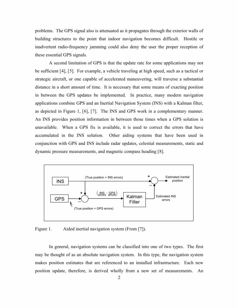
A second limitation of GPS is that the update rate for some applications may not

be sufficient [4], [5]. For example, a vehicle traveling at high speed, such as a tactical or

strategic aircraft, or one capable of accelerated maneuvering, will traverse a substantial

distance in a short amount of time. It is necessary that some means of exacting position

in between the GPS updates be implemented. In practice, many modern navigation

applications combine GPS and an Inertial Navigation System (INS) with a Kalman filter,

as depicted in Figure 1, [6], [7]. The INS and GPS work in a complementary manner.

An INS provides position information in between those times when a GPS solution is

unavailable. When a GPS fix is available, it is used to correct the errors that have

accumulated in the INS solution. Other aiding systems that have been used in

conjunction with GPS and INS include radar updates, celestial measurements, static and

dynamic pressure measurements, and magnetic compass heading [8].

Figure 1. Aided inertial navigation system (From [7]).

In general, navigation systems can be classified into one of two types. The first

may be thought of as an absolute navigation system. In this type, the navigation system

makes position estimates that are referenced to an installed infrastructure. Each new

position update, therefore, is derived wholly from a new set of measurements. An

INS

Kalman Filter

GPS

+

_

+ _

(True position + INS errors)

(True position + GPS errors)

Estimated INS errors

Estimated inertial position

errors errorsINS GPS

3

attractive feature of this type of system is that errors that occurred in past position

estimates do not propagate into future estimates. A disadvantage, however, is that this

type of navigation system requires good “line-of-sight” to the infrastructure. Examples

of theses types of systems include GPS, Loran-C, and celestial navigation.

Alternatively, a relative (or incremental) navigation system is one where new

position estimates are computed with respect to previous ones. Often, this is called dead-

reckoning navigation. The INS is an example of this type of position tracking system,

wherein acceleration measurements are doubly integrated at the end of each sample

interval to derive position. A well-known limitation of this type of system is that position

errors tend to grow, and the system must be periodically reinitialized. An advantage, on

the other hand, is that the relative navigation system does not require the use of an

infrastructure; therefore, it can be used in those places where the infrastructure of the

absolute navigation system is unavailable.

Lastly, a third and final form of the navigation system is a hybrid, as shown in

Figure 1. It combines the attributes of the absolute navigation system with those of the

relative navigation system.

B. SENSORS FOR INERTIAL NAVIGATION

Perhaps the first to recognize the utility of a self-contained system for guidance

and navigation of a vehicle were the Germans during WWII, when they assembled gyros

and accelerometers into a platform and installed the resulting inertial measurement unit

(IMU) into V-2 rockets to deliver a deadly payload to targets lying across the English

Channel in England [9]. Immediately after the war, the United States, impressed by the

German’s technological achievement of the rocket’s IMU, initiated an engineering

program to further study and improve the design. As a result, the modern IMU has

evolved into a highly complex system of precision mechanical assemblies, electronics,

and advanced algorithms. In their present form, the IMU is manufactured in one of two

varieties: the platform IMU and the strapdown IMU. Both variants contain two or three

mutually perpendicular accelerometers for measurement of motion along a defined set of

reference directions.

4

A main distinction between the two architectures, however, lies with the manner

in which the acceleration measurements are accomplished. In the platform IMU, gyros

are used to stabilize the axis of an accelerometer and align it with that of a navigation

reference frame. More specifically, the spin axes of a set of mutually perpendicular

gyros—having a very large angular momentum and tending to resist any change in their

orientation—are aligned with the axes of a navigation reference frame. The gyros are

mounted into a cage such that their axes may tilt freely relative to the cage (and vehicle)

in which they are mounted [9]. As the vehicle orientation changes during the course of a

mission, the gyro axes remain fixed and aligned with the navigation reference frame.

Consequently, the accelerometers, whose alignment have been preserved with that of the

navigation frame, produce measurements of motion already referenced in the desired

navigation coordinate system. It then becomes a simple matter to doubly integrate these

measurements to derive the new position.

Alternatively, a strapdown IMU is one in which the accelerometers are “strapped”

to the vehicle body. As such, as the vehicle pitches, rolls, and yaws, so do the axes of the

mutually perpendicular accelerometers. The resulting measurements of acceleration are

consequently referenced in a body frame and not in the required navigation frame. Gyros

are used in this mechanization to measure body rotational rates [10]. From these

measurements, the vehicle orientation is derived and subsequently used to reference the

acceleration measurements in the navigation frame. Then, in a similar fashion to the

platform IMU, the properly referenced accelerations are doubly integrated to derive a

position.

Platform IMUs tend to be large and heavy. They are constructed of mechanical

moving parts and require periodic maintenance to maintain the mechanical hardware in

good working order. Their use is primarily reserved for high-accuracy applications and

long range missions. Strapdown IMUs, on the other hand, tend to be smaller and lighter

than the platform IMU. They also require less power to operate and cost less than the

platform IMU. A disadvantage of the strapdown IMU, however, is that greater

computational effort is required because of the requirement to resolve the accelerometer

measurements in the navigation frame before integration.

5

C. MEMS TECHNOLOGY

Micro-electro-mechanical systems (MEMS) technology has enabled the

miniaturization of various types of common sensors. Sensors that have been

manufactured with MEMS technology, such as accelerometers, rate gyroscopes, and

pressure sensors, are much smaller than those manufactured with conventional

macroscale techniques (welding, casting, machining). MEMS-based sensors are

manufactured with mature microelectronic manufacturing processes. As a result, the

sensing element can be combined into the same substrate with required signal

conditioning and signal processing electronics. Typical electronic processes that may be

applied to a sensor signal include biasing, low-pass or high-pass filtering, amplification

(scale and offset), analog-to-digital conversion, or even self-diagnostics of the sensor

[11].

The MEMS-based sensor has found a wide array of applications due to its smaller

size, lighter weight, and lower power consumption. For instance, the automobile industry

has successfully integrated MEMS accelerometers into their vehicles for crash detection.

More recently, the rate gyroscope has been used in a new feature of automobiles called

vehicle stabilization [12], [13].

1. Survey of MEMS Devices

MEMS devices beyond those of accelerometers and gyroscopes have been

developed. Honeywell, Inc., manufactured an infra-red thermal imaging sensor that is

capable of operation at room temperature [14]. A carbon monoxide gas sensor called the

MGS1100 was manufactured by Motorola, Inc. [15]. Knowles Acoustics, Inc.,

developed the SiSonic microphone. The major advantage of this type of microphone is

the fact that it can be integrated into automated printed circuit board fabrication assembly

lines that operate at elevated temperatures [16]. The more common electret microphone,

which is not capable of withstanding these elevated temperatures, must be installed by a

secondary assembly process, adding time and cost to the overall assembly.

Still, other devices beyond sensors have been manufactured with MEMS

technology. Texas Instruments invented a micromachined steerable mirror that it has

6

successfully marketed for use in projection displays, [17], [18]. A more ubiquitous use

of MEMS technology is found in the ink jet printer. IBM patented a number of designs

for silicon nozzles used to reliably deliver precise amounts of ink [19], [20], [21]. An

optical switch for use in a fiber optic network employing wavelength division

multiplexing has been patented by several companies including Optic Net, Inc. [22],

Fujitsu Laboratories [23], Agere [24], and Xerox [25]. If a MEMS device is built upon a

gallium arsenide substrate rather than silicon, then devices suitable for operation above

1 GHz can be manufactured. Radio frequency MEMS, or RF MEMS, such as switches,

antennas, and variable capacitors have been developed in the laboratory [26]. A

thorough discussion of the many MEMS applications is exhaustive, nevertheless, [11]

and [27] are good references to begin an in-depth survey of the many areas that have

benefited from MEMS technology or are postured to benefit in the future.

2. An IMU Based on MEMS Technology

The widespread use of the MEMS-based accelerometers and gyros in the

automotive industry has reduced the cost of these sensors to the point that they become

attractive for use in other applications—most notably the Apple iPhone and the Nintendo

Wii-mote. The former uses these sensors to determine the orientation of the display and

to detect finger taps. Nintendo’s Wii-mote incorporates this type of sensor for motion

sensing and gesture recognition to interface with a video game [28].

In 2001, Marins et al. began building prototypes of a miniature strapdown IMU

with accelerometers and gyros [29]. The prototypes also included magnetometers for

measurement of heading. This concept appealed to a number of manufacturers, including

XSense, Microstrain, and MEMSense, which developed their own versions of the

miniature IMU for the commercial market; see Figure 2. These units alleviated the

researcher from having to design his/her own custom printed circuit boards for

integration and packaging of the sensors. The commercial units addressed all of the

technical issues related to the filtering and sampling of the sensor signals, as well as the

precise mechanical alignment required for the sensors. These units generally

incorporated a microcontroller to handle the analog-to-digital conversion, processing, and

7

formatting of the sampled data for subsequent transmission via any number of means,

including RS-232 or I2C. Upon assembly at the manufacturer facility, all of the essential

calibration and compensation constants could also be programmed into the

microcontroller to improve the overall accuracy of the reported sensor data.

Because of their light weight, small size, and low power, one of the applications

for which these units are suitable is personal navigation. A miniature inertial/magnetic

measurement unit (IMMU) may be worn by a user, and as he/she moves about from one

place to another, the sensed accelerations could then be processed to track their position

in a manner that is very similar to strapdown navigation. A limitation of this approach,

however, deals with the quality of the MEMS-based sensors compared to their

conventional counterparts found in the navigation-grade IMU. The MEMS-based

accelerometers and gyros exhibit more noise than those sensors used in navigation-grade

systems [30], [31]. Table 1 compares the MEMS-derived accelerometers and gyros with

those of the LN-200, which is a navigation-grade IMU manufactured by the Northrup-

Grumman; it is used in a number of military systems such as Predator, Global Hawk, and

the AIM-120 Advanced Medium Range Air-to-Air Missile [32]. The added noise

possessed by the MEMS-based sensors will cause the position error in the personal

navigation application to grow rapidly. Consequently, the development of innovative

algorithms beyond that of the accepted strapdown navigation algorithm will be required.

8

Figure 2. Miniature IMMU from Microstrain, Inc. (From [33]).

Table 1. Comparison of Noise in Navigation-Grade Sensors and MEMS Sensors.

Accelerometer Angular Rate Sensor

Nav-grade Northrop-Grumman A-4 Triad

5 / Hzg Fiber-Optic Gyro (LN-200)

0.07 /o hr

MEMS Analog Devices ADXL325

250 / Hzg Analog Devices* ADXRS610 [33]

3.0 /o hr

* Analog Devices, Inc., specified the noise density of its sensor in units of [ o /s/ Hz ]. The

ADXRS610 has a noise density of o0.05 /s/ Hz . This figure was converted into units of ohr/ using the

following expression: o o1

60[ / hr ] [ /hr/ Hz ]ARW NoiseDensity

where the noise density specified by Analog Devices was first multiplied by 3600 sec/hr to set the figure into the proper units.

3.5”

2.5”

9

D. PERSONAL NAVIGATION

While position tracking solutions utilizing GPS and the INS have been

implemented with great success on maritime and aerospace vehicles, the transition of this

concept to the problem of tracking the position of an individual is in its infancy. One

may argue that such an approach to this problem is unnecessary and that a personal

navigation system based solely on GPS is sufficient. However, for reasons stated

previously, namely the availability of the GPS signal (or lack thereof), there is a strong

case for using inertial/magnetic measurements in a personal navigation application. This

concept is valid in situations where the GPS signal can not be received. Additionally,

since it is uncertain how long the GPS signal may be unavailable during the course of a

pedestrian trip, there exists the need for an IMMU implementation that is reliable and

robust to compensate for the GPS downtime.

A main component of this body of work deals with the subject of personal

navigation. Subsequently, it is worthwhile to spend a moment expanding on the

definition of the subject. Personal navigation in this context refers to the tracking of

one’s position. A recent article found on the internet [34] suggests that modern personal

navigation is based solely on the use of handheld GPS devices. However, there are other

ways that one could perform the task of personal navigation. Making observations of

landmarks and correlating them to a map of the region, as had been done for millennia, is

certainly a valid approach. Therefore, the term, personal navigation, does not imply

which technique is used to accomplish this task. In the context of this work, however,

personal navigation refers to the use of inertial measurements in a dead reckoning scheme

to establish the position of an individual.

1. Applications for Personal Navigation

There are a number of potential applications for the personal navigation

technology, both military and civilian. The Marine infantry learn in training how to track

their position using nothing more than a map and a magnetic compass. However, this

technique is limited by the fact that good line-of-sight to mapped landmarks is required.

In dense jungle or heavily forested areas, the line-of-sight to these landmarks may not

10

exist, and the aid of GPS may be unavailable. A personal navigation system tailored for

infantry use could prove itself useful in this situation. Still another military application

could be found in the potential increase in situational awareness offered to a team of

marines or soldiers in a tactical situation. Knowledge of the location of fellow team

members in a building or other urban combat setting could improve the overall situational

awareness and increase the likelihood of a successful mission outcome.

Still another potential application for a personal navigation system pertains to

assistance for the vision impaired [35]. GPS-based solutions have been developed. In

[36] and [37], GPS information is integrated with a location database to give the user

audible cues to a desired destination. The IMMU-derived data could be integrated with

the GPS information to give the user a more accurate position solution and provide a

means of navigation during those times when the GPS signal is unavailable, for example,

when walking inside a residence or a shopping mall.

The coordination of emergency rescue operations is yet another area to benefit

from the development of a personal navigation capability. Given accurate location

information of emergency medical technicians, an emergency dispatcher can effectively

direct the services to the location of those in need. The position data could be

superimposed onto a building floor plan, if desired, to assist the dispatcher in guiding the

rescuers to the appropriate location.

A personal navigation system would not necessarily be limited to these

applications. With the advancement of engineering control systems applications, a new

type of robot has emerged, a true walking robot, like Asimo manufactured by Honda

Corp. Asimo is one of the first robots of this type to integrate a feedback control system

to ensure that the robot is able to maintain its balance as it walks. Furthermore, the robot

is able to shift its center of gravity and rotate its hips, as required, to coordinate turns as it

travels [38]. This provides the robot with a smoother, more human-like motion.

Wheeled robots, which are the predominant type of robot with a locomotion capability,

use encoders on their wheels to track their position as they move about a space.

However, walking robots, such as ASIMO, must use some kind of “step counting”

technique to determine their position in a room. As the robot emerges from the

11

laboratory and into the real world, a personal navigation system could potentially offer

some alternative means of navigation within a larger space.

The impetus for research in this area came from ongoing work by Yun et al. at the

Naval Postgraduate School in support of a U.S. Army sponsored program to develop a

posture tracking capability for training in a virtual environment. A detailed description of

this work is found in [39], [40], [41], [42], and [43]. With the development of a personal

navigation capability, another level of realism can be created within the virtual

environment. Through the incorporation of accurate position data into the virtual

environment, a more realistic training experience may be envisioned.

2. Objective for Personal Navigation

The primary objective of this dissertation is to develop a personal navigation

system (PNS) that uses the miniature IMMU. The PNS will require the user to carry an

IMMU on his/her foot. Accelerations induced by natural walking motion will be

processed to derive an updated position of the user. The strapdown navigation algorithm

will be adapted for this application. It will utilize an adaptive-gain quaternion-based

complementary filter that was specifically tailored for the PNS. Furthermore, the

strapdown algorithm will incorporate the concept of zero-velocity updates and a custom

gait-phase detection algorithm to determine the instances of the foot swing and stance

periods.

The PNS will be constrained for use only during normal biped walking.

Locomotion by other means (i.e., limping, skipping, hopping) was not considered in this

dissertation, but are topics for further study and development. Performance of the PNS

was initially examined for the case of running motion. It was found that the data sample

rate was insufficient to identify the necessary features of this type of locomotion and was

not considered beyond this point.

An additional operational limitation of the PNS deals with the walking surface.

Only flat, level walking surfaces were examined, such as concrete or other types of

manufactured flooring (tile, rubberized asphalt). Walking on softer surfaces such as grass

made it difficult for the gait-phase detection algorithm to determine the essential features

of natural walking motion.

12

One more limitation of the PNS deals with the fact that it was only tested by the

author. Therefore, all the parameters that were adjusted in the PNS—there are a number

of thresholds and gains used throughout the system—were chosen to give the best tracks

for data that was collected by the author while walking with the miniature IMMU

attached to his foot. Additional consideration will be required to determine whether or

not the selected parameters are suitable for a larger set of users.

E. LOCOMOTION INTERFACE FOR THE VIRTUAL ENVIRONMENT

A virtual reality is a computer-generated environment intended to provide a

medium for one or more persons to interact in some manner—either with one another or

with the environment itself. The virtual reality incorporates features such as computer

graphics, sound, tactile feedback (haptics), smell, and any number of other user

interfaces, including keyboard and computer mouse to enhance the interaction with the

user [44]. Undoubtedly, the most common application of virtual reality is entertainment

[45]. Popular with the younger generation, the annual global sales of video games are

estimated to be $12 billion [46]. Another use of virtual reality is found on the World

Wide Web. Approximately 50 million people have created avatars to engage in this

virtual social network [47]. Non-entertainment applications of virtual reality exist, as

well, for use as training simulators, educational tools, as part of a therapeutic regimen, or

to aid in the visualization of an engineering or scientific problem [48], [49], [50].

The military has a demonstrated interest in using virtual reality. Military training

programs that have a component within virtual reality can be provided at reduced cost

and with the added benefit of enhanced safety [51]. For example, combat training with

live ammunition is costly and presents additional risks to soldiers. Training in a virtual

environment can reduce some of the costly burden and mitigate some of the safety risks

associated with this type of training. While training entirely in the virtual world is not a

suitable substitute for real-world training, it offers an opportunity for an acceptable level

of compromise. Another attraction of training in a virtual environment is that many

soldiers of the younger generation have grown up playing video games. In this regard,

they feel quite comfortable interacting with a simulated reality for training purposes, see

Figure 3 and [52].

13

Figure 3. Navy personnel in a virtual reality parachute trainer wearing a head-mounted display (From [53]).

Furthermore, the military, both U.S. and foreign, has employed training

simulators to educate personnel in the operation of advanced weapons systems, such as

tanks and aircraft. For these types of weapon systems, training in the virtual

environment reduces overall cost because it decreases fuel consumption and maintenance

requirements due to the reduced operation of the real weapon system. Moreover, the

safety of personnel and equipment is increased because they have some exposure to the

system operation before the actual hands-on experience. An added benefit of this type of

training is that it reduces the overall environmental impact because the actual weapon

system does not have to be used in the field as often [53], [54].

Another military application for virtual reality is in the treatment of post traumatic

stress disorder (PTSD) [55]. In this approach to PTSD therapy, the patient is gradually

introduced to the sensory details (visual, sound, and scent) in a virtual reality of the

trauma with the motivation that he/she will learn to manage the effects of the disorder.

This type of regimen, also known as a form of prolonged exposure therapy, has the

benefit in that it can be administered in the safe environment of the doctor’s office. In the

past, treatment for this type of disorder may have required that the patient confront the

source of the trauma or fear in a real-world setting, thus placing the patient (and attending

staff) in a potentially hazardous situation. With virtual reality therapy, however, the

14

exposure can be accomplished in a safe location with all of the sensory stimuli introduced

in a controlled manner at the doctor’s discretion. An initial experiment of this approach

was conducted in 1997 on Vietnam veterans suffering from PTSD. The experiment

showed positive results, and the treatment has been advanced for use in Iraq war veterans

suffering from the same disorder [56].

1. Immersion and Presence

For a user to feel as an integral part of the computer-created virtual world, he/she

must have a sense of presence when interacting with the virtual environment. That is,

presence is the subjective measure of one’s feeling that he/she is in the virtual reality

[57]. Furthermore, presence is dependent on the level of immersion that a virtual

environment is able to offer. Immersion, on the other hand, is the objective measure of

the amount of sensory stimuli that is provided by the virtual environment. For example, a

virtual reality that uses detailed graphics displays, sound, and advanced user interfaces

will offer a higher level of immersion than one that only provides a low-resolution

display of the virtual environment without any other sensory stimuli. Consequently, for a

user of a virtual training program (or therapeutic regimen) to have a positive or rewarding

experience in a virtual environment, he/she must have a high sense of presence. In turn,

the high presence can only be achieved through an adequate level of immersion, which is

provided by the various forms of interfaces available to the user.

To that end, researchers and commercial developers have made interfaces of

various types to heighten the experience within the virtual environment. Sound and

graphics systems are the most common, but locomotion interfaces have also been

developed. A locomotion interface gives the user control of his movement through the

virtual environment. Many are variations of treadmill designs, assumedly because this

requires user body motions most like those required in the real world and would most

likely result in a high sense of user presence. Other designs for locomotion interfaces are

based on step-in-place devices where the user steps on pads located on the floor to direct

his/her motion through the environment.

15

2. Objective for the Locomotion Interface

In dealing with the subject of virtual reality, an objective for this dissertation is to

develop a locomotion interface for the virtual environment incorporating the miniature

IMMU. The locomotion interface will allow a user to navigate within a virtual

environment. A miniature IMMU will be worn on each foot; a custom C++ application

called MOVESMover interprets the user’s foot gestures to direct his translation through

the virtual environment. The user is allowed to move forward, walk left/right, side-step

left/right, and turn-in-place clockwise or counter-clockwise. Systems that utilize large

displays where the user remains fixed in one location are suitable for this type of

interface. Specifically, the locomotion interface was designed for a marksmanship

training system that projects virtual targets onto a large projection display located

immediately in front of the trainee.

A limitation of this interface, however, is that the user is not allowed to move

backwards through the virtual environment. In spite of this, the user can turn-in-place to

face the opposite direction, then walk forward to achieve a similar translation. A second

limitation is that the interface only operates in one speed. The pace of the foot gestures

could not be interpreted accurately with our MOVESMover program. Consequently, the

speed was programmed to one value only.

F. DISSERTATION OUTLINE

This dissertation primarily focuses on the development of the PNS, but a chapter

is dedicated to explaining the design and operation of the locomotion interface that was

developed for a virtual environment, which also utilizes the miniature IMMU.

Background material relevant to the subsequent chapters is presented in Chapter II. It

introduces the zero-velocity updates and the gait-phase detection algorithm. An

introduction to the quaternion and its role in the strapdown navigation algorithm is also

included here. The Factored Quaternion Algorithm (FQA), which is used for orientation

estimation, is presented in Chapter III. Additionally, the manner in which the FQA is

integrated into the complementary filter to give improved dynamic performance is also

discussed in this chapter. The PNS and all of its component algorithms are presented in

16

Chapter IV, along with a summary of its performance. In Chapter V, the novel

locomotion interface is presented, which was a by-product of the research work carried

out in pursuit of the PNS. Lastly, conclusions and recommendations for future research

are provided in Chapter IV.

17

II. BACKGROUND AND PRELIMINARY WORK

This chapter presents material relevant to the development of the PNS. Since the

subject of this dissertation deals in large part with human walking motion, it is

worthwhile to begin this chapter with an examination of the salient features of

ambulatory locomotion. After this, a brief review of related work is outlined, as well

as,previous work that was conducted at the Naval Postgraduate School. This chapter also

introduces the concept of the zero-velocity updates and the gait-phase detection

algorithm, two essential components that are integrated into the strapdown navigation

algorithm and adapted for use in the PNS. The chapter concludes with some initial trials

of the PNS and highlights the need for a quaternion-based orientation algorithm that is

tailored for this particular application.

A. HUMAN GAIT CYCLE

Walking is the most natural form of locomotion. It is a highly complex

coordinated movement of our feet, legs, hips, arms, and torso to propel our center of mass

in a forward direction. Walking is an innate ability we acquire not too long after we have

developed sufficient motor skills to perform this articulated motion. The average age one

learns to walk is 11 months. Generally, the details of walking are given very little

consideration. That is to say, most of us pay little attention to how the different parts of

our body move when we are walking, what muscles are involved, or how we balance and

control the location of our center of gravity. Walking is second nature. However, an

understanding of human walking motion is important because it relates to the analysis of

the normal gait cycle and to the identification and treatment of neurological and

physiological disorders. A detailed study of this complex motion would be exhaustive,

involving at the very least the fields of anatomy, physiology, and biomechanics.

Fortunately, for our purposes, we require only a simplified analysis of this complex body

motion.

The gait cycle of normal human walking is defined as the interval of motion from

heel strike to heel strike of the same foot [58]. Figure 4 shows an example of one cycle

18

of normal human walking motion. At the left of this diagram, the human figure begins a

gait cycle at the moment the heel of the right foot strikes the ground. The gait cycle

continues through several distinct phases, such as, the toe-off phase of the left foot, heel

strike of the left foot, toe-off phase of the right foot, and concludes with another heel

strike of the right foot. Alternatively, the gait cycle may be analyzed with regard to the

motion of the left foot. Figure 4 further shows how ambulatory motion consists of two

fundamental phases: a stance phase and a swing phase. The stance phase of either foot is

the interval between its heel strike and toe-off. It represents the period that this foot is in

contact with the ground. A complete gait cycle, therefore, has two stance phases, one

corresponding to each foot. The stance phase occupies approximately 60% of the normal

gait cycle.

Figure 4. Phases of the human gait cycle (From [59]).

The swing phase is characterized by the fact that the foot does not bear any

weight during this interval. In this phase, the foot begins accelerating at the moment of

toe-off until a maximum acceleration is reached somewhere in mid-swing, at which time

19

deceleration begins to slow the foot velocity in preparation for the subsequent heel strike.

There will be two swing phases in a given gait cycle. This interval occupies

approximately 40% of the normal gait cycle.

A double support phase is another characteristic of normal walking motion. This

is the interval of normal walking when both feet are in contact with the ground. There

are two such periods of double support in each gait cycle. At faster walking speeds, the

double support period decreases and disappears altogether at the onset of running motion.

Whether the motion is walking at slow or moderate speeds, or running at fast

speeds, most of the motion generally occurs in the sagittal plane of the human body. The

predominant amount of motion of the feet and legs coincides with this plane. Figure 5

shows the location of the sagittal plane, along with the transverse (or horizontal) plane

and the frontal plane. Normal walking consists of body motion beyond that of the feet

and legs, however. The pelvic bone also exhibits some motion in support of normal

walking. The pelvis will rotate in the transverse plane and tilt downward in the frontal

plane during the course of walking. The torso will also exhibit some motion in these

planes. Because of their inertia, the arms will appear to rotate in the sagittal plane as the

center-of-mass moves forward—creating the appearance that the arms are swinging.

Some of the more common parameters used to describe the normal gait cycle are

the stride length, walking speed, and cadence. Stride length measures the distance

traversed of a given foot in a particular gait cycle. It is approximately half of the step

length, where the step length is the distance separating the feet during the double support

phase. Walking speed is a scalar quantity that gives the rate of travel of the center-of-

mass. Lastly, cadence is reported in number-of-steps per unit of time. These parameters

are used in the analysis of the human gait cycle and diagnostics of related disorders.

They are highly dependent on individual features, such as, stature, weight, age, and

gender.

20

Figure 5. Planes of body motion (From [59]).

B. RELATED WORK

Small, lightweight accelerometers and gyros have been used in the past to study

human body kinematics. Among the various motivations for this research was a need to

assess physical activity and its relationship to energy expenditure [59]. Others have

sought to classify body motion patterns and relate these measurements to biological and

psychological data, such as, gender, emotion, and personality [60]. Still, other

applications concern the rehabilitation of those suffering from injuries or disorders

affecting normal walking behavior, for example, as in the development of a

neuroprosthesis to alleviate “dropped-foot” syndrome, as described by Pappas et al. [61].

1. Related Works Using Small Lightweight Sensors

In Pappas et al., the researchers demonstrated a gait phase detection system that

merged angular rate data from a gyro attached at the heel of a shoe with data from a set of

force sensitive resistors glued to the insole of the same shoe. These data were then fed

21

into a state machine to determine the corresponding phase of a particular gait cycle:

stance phase, heel-off phase, swing phase, or heel-strike phase. The system was reported

to have an accuracy of 99% for determining the gait phase during walking motion,

ascending or descending stairs, walking on inclines, and running for short periods. This

information was then used to stimulate muscles used to elevate the foot during a given

swing phase.

With regard to personal navigation, various approaches have been introduced.

Some have the sensors attached at the waist or torso and used a combination of inertial

sensors and other navigational aids. For example, Lee from Korea and Mase from Japan

collaborated on several papers that explored different techniques to assess walking

features, determine distance, or compute position. In [62], they utilized a two-axis

accelerometer, a digital compass, and an infra-red beacon system to aid in landmark

recognition. The sensors were arranged in a small enclosure worn on the waist of the test

subject. The researchers focused on a scheme to count steps and identify whether the test

subject was walking on level ground, walking up, or walking down a stairway. They

examined the use of the cross-correlation of the x-axis and z-axis accelerometer as a

means to establish one of the three types of ambulatory motion. The researchers reported

the ability to identify level walking and climbing down stairs with more than 95%

success and climbing up stairs with 83% success. They also proposed an algorithm to

determine stride length based on the time between observations of peak accelerations, but

no experimental results were presented.

In [63], the same collaborators used an arrangement of four orientation sensors

(one on each thigh and one on each leg) to determine stride length. The orientation

sensors manufactured by NEC Tokin, model MDP-A3U9 consisted of three

accelerometers, three angular rate sensors, and three magnetometers to provide three-

dimensional orientation of each limb. They used the data from these devices in a biped

stick model of the human figure to calculate the stride length after each step. The model

related the measured orientation (Euler angles) of each limb in a trigonometric manner to

22

tep length. The authors reported a 2.3% average error in step length estimation based on

the limited testing of this sensor arrangement on one test subject during a trial that

consisted of walking 30 steps.

In another work by the same researchers, they explored some techniques to

recognize whether the subject was sitting or standing, climbing stairs, descending stairs,

or walking on level ground [64]. When the algorithm identified level walking, it then

tried to establish walking speed (slow, normal, or fast). The sensors used were a two-axis

accelerometer and one rate gyro, which were carried in a small box and inserted into the

pocket of one’s trousers. An electronic compass whose output consisted of one of four

discrete values representing the directions of north, south, east, or west was worn on the

waist. In order to classify the type of motion (i.e., sitting, standing, walking) Lee and

Mase organized the sensor data into a “feature vector” that was used in a fuzzy logic

scheme. They reported better than 92% success for the task of motion recognition.

In this same work, the researchers developed a method for location recognition

that was based on a table look-up of presurveyed locations in an office space. A

displacement vector with the number of steps taken in each direction was used for input

to the look-up table. The authors also reported good results with this technique from the

testing of one individual.

Researchers have also investigated attaching sensors to the foot. While this may

be considered a more inconvenient location for the sensors than the waist or torso, this

offers the opportunity for mitigating some of the errors in the computed position due to

the occurrence of the foot’s zero velocity during the stance phase. Sagawa et al. in [65]

reported good results when they computed distance walked using this drift correction

technique that was applied to data derived from a foot-mounted three-axis accelerometer.

In addition to the three-axis accelerometer, the experimenters used an angular rate

gyroscope, also attached to the same foot. The phase of the gait was detected by

comparing the foot angular velocity with a specified threshold. The acceleration was

integrated to produce velocity, and then a correction was applied to this result to

compensate for the error that had accumulated during the swing phase. Another

integration of the corrected velocity data produced the calculated distance. An average

23

computed distance of 30.0 + 0.8 m was reported for eight test subjects walking at various

speeds over a 30.0 m path. The error correction applied to the velocity data was based on

the fact that at the end of the swing phase, the foot comes to rest on the ground and will

have a zero velocity. By identifying this point in the velocity profile (i.e., where the foot

had come to rest) an opportunity was provided for correcting the error that had

accumulated during the integration of the acceleration data.

Similar work was described by Cavallo and Sabatini in [66]. This work sought a

technique to identify gait cycles with a foot-mounted IMU that consisted of a two-axis

accelerometer and a single-axis angular rate gyro. Tests were conducted on a number of

subjects walking on a treadmill machine. The authors determined velocity and incline of

the treadmill from the measurements of acceleration and angular velocity. They

employed a “resetting” algorithm to account for the sensor errors resulting from the

integration of the noisy sensor data. This algorithm made use of the zero foot velocity

and provided an opportunity for recalibration of the sensor. In a subsequent work, the

same group of researchers explored a GPS/INS implementation of a personal navigation

system [67]. They compared IMU-calculated distance with GPS-computed distance to

verify that good results could be achieved through the integration of the accelerometer

data. Heading was derived from the GPS information to produce a position tracking

capability.

Randell, Djiallis, and Mueller presented an alternative approach to personal

navigation in [68]. They experimented with different configurations of a two-axis

magnetic compass and a single-axis accelerometer to determine position. The

accelerometer was attached to the foot and used to make estimates of stride length. The

authors proposed that there was a correspondence between the peak vertical acceleration

of the foot and the stride length. In this manner, the technique avoided the integration of

any sensor noise in the accelerometer. The authors reported good results in the

assessment of traveled distance, but stated that the two-axis magnetic compass did not

yield reliable heading information, especially in the urban environment. The authors

indicated that this was likely due to anomalous variations in the magnetic sensor data and

24

that the sensor could not be maintained in a level position during the experiments. They

further reported that a three-axis magnetic compass would be able to provide a means of

tilt compensation and yield better results.

2. Related Work at the Naval Postgraduate School

At the Naval Postgraduate School, in Monterey, California, researchers have been

involved with the development and testing of sensors for the purpose of inserting one’s

body orientation into a virtual training environment. The prototype devices were

miniature IMMUs, which were assembled with accelerometers, gyros, and

magnetometers.

Bachmann in [39] described the development and testing of a miniature IMMU

for use in posture tracking. The devices were attached to the limbs of the subject. Data

from the sensors were merged in a complementary filter to produce a 3-D measurement

of orientation for each instrumented body segment. A virtual image (avatar) was then

generated that reproduced the posture of the individual. Figure 6 shows the concept of

the system, and Figure 7 shows Bachmann demonstrating the use of the miniature IMMU

sensors to orient the virtual avatar. This work was the impetus for the study and

development of the PNS at the Naval Postgraduate School.

Figure 6. Conceptual tracking system (From [39]).

25

Figure 7. Bachmann demonstrating the MARG sensor and the avatar.

Sensors are attached to subject’s leg to measure its orientation (From [39]). Recently, Moore in [69] explored the use of the Microstrain 3DM-GX1 sensor

(Figure 2). Like the custom prototypes used by Bachmann, the commercially-available

3DM-GX1 was a miniature IMMU. However, its built-in microcontroller calculated

sensor body orientation from the raw data and made this data available through its serial

communications port. This alleviated the user from having to develop an algorithm to

calculate the orientation angles. The raw sensor data from the accelerometers,

magnetometers, and rate gyros were also available to the user through the same

communications port. Moore initially used this sensor in the same fashion as Bachmann

to provide orientation or posture data for an avatar. Later he attached the sensor to his

foot to collect dynamic data of ambulatory motion. The data collected from these latter

experiments were analyzed to determine his position (distance and direction traveled)

from an arbitrary starting point. Moore concluded in his thesis that these sensors were

viable for use in personal navigation applications. However, due to the errors inherent in

the sensor data and the numerical integration of the corresponding data, additional effort

would need to be expended to develop their use in a practical personal navigation system.

Two important ideas that Moore explored were the application of the zero

velocity updates and the use of the gyro to detect the swing and stance phases of the foot.

26

In the next two sections, the concept of the zero velocity updates and the gait-phase

detection algorithm are presented. They will become essential components in the PNS.

C. ILLUSTRATION OF ZERO VELOCITY UPDATES

One of the first tests that Moore conducted was to simply move the MARG sensor

through a straight line. Here, the sensor was placed on a table top and slid through a

linear distance of one meter. Figure 8 shows the results from this test. Acceleration is

seen in the top-most plot. In this test, the sensor was stationary for approximately six

seconds prior to its translation across the table. After its trajectory was completed, the

sensor was kept stationary for another seven seconds, approximately. The acceleration

appears relatively small during the stationary periods, while the acceleration occurring

during the sensor’s translation is clearly observed within the time period between six and

eight seconds. A numerical integration of this data (using Matlab’s cumtrapz( ) function)

produced the velocity plot, also shown in Figure 8. Similarly, integrating the resulting

velocity data gives the final distance of 12.44 meters—a considerable error when

compared to the actual distance of one meter.

27

Figure 8. Result of one meter translation of IMMU (From [69]).

Upon closer inspection of the velocity plot, one observes that prior to the sensor’s

motion, as well as immediately after its motion, the velocity is nonzero. Integration of

this nonzero data in the velocity is responsible for the gross error in the computed

distance. These errors arise because the accelerometer’s output exhibits two behaviors

that must be taken into consideration—bias and drift. Bias is the nonzero output

measured when the accelerometer undergoes no acceleration. Drift is the randomly

varying portion of the sensor output often referred to as noise.

These errors may be mitigated through a two-step process. First, since the sensor

undergoes no acceleration outside of the time period between six and eight seconds, the

acceleration during those times may be equated to zero. Subsequent numerical

integration of the data will eliminate this component of error.

28

Secondly, the measured acceleration between six and eight seconds will also be

influenced by the sensor bias and drift. To minimize this effect, the zero velocity update

was employed. The measured acceleration, am(t), consists of two components such that

( ) ( ) , [0, ]m aa t a t t T (2.1)

where aa(t) is the actual or true acceleration and is a bias error that is assumed constant

in the time interval over which the acceleration occurred. In the example under

consideration, t=[0,T] corresponds to the time period between six and eight seconds.

Integration of am(t) will yield a calculated velocity, vc(t), as shown in (2.2).

( ) ( )

( )

( ) , [0, ]

c m

a

a

v t a t d

a t d d

v t t t T

(2.2)

The calculated velocity, vc(t), is comprised of two parts. One component, va(t) is

the true velocity that is derived from the true acceleration. The other component, which

is the product of and t, arises from the error in am(t). However, at the end of the

accelerated motion, when t=T, the motion has stopped, and the true velocity, that is va(t),

is known to be zero. Substitution of this fact ( va(T) = 0 m/s ) into the latter part of (2.2)

gives the expression for the error that is valid during the interval t=[0,T].

( )cv T

T (2.3)

The numerator in (2.3) is taken from the last sample of vc(t), when t=T.

Substitution of (2.3) into (2.2) and solving for va(t) gives an expression that is used to

correct the velocity data for the error encountered during the interval of the accelerated

motion, as shown in (2.4).

29

( )

( ) ( ) , [0, ]ca c

v Tv t v t t t T

T (2.4)

With the actual velocity data in hand, a final integration of the data produces a

revised figure for the distance traveled. Figure 9 shows the corrected data plots and a

new calculated distance that is more acceptable than previously calculated. Moore

repeated this test for distances of two and three meters, the results of which are shown in

Table 2. The distance errors of 0.5% and 0.33% for the two- and three-meter tests,

respectively, are noteworthy in that they validate the technique for correcting the drift and

bias inherent in the accelerometer data.

Figure 9. Result of one-meter displacement of IMMU after data was corrected for error (From [69]).

30

Table 2. Results of linear displacement of IMMU (From [69]).

Measured Distance (m) True Distance (m)

Uncorrected Corrected

Corrected Distance

Error

1 12.44 1.00 0.0%

2 -1.45 2.01 0.5%

3 -2.57 2.99 0.33%

D. GAIT-PHASE DETECTION ALGORITHM

To utilize the zero velocity updates in a PNS, the IMMU was attached to the

user’s foot. It is here that a zero velocity is certain to occur during the stance phase of

normal walking. In this brief moment, the zero velocity can be identified and the

correction to the velocity profile applied as illustrated in the previous section. The first

trial of this concept in the navigation application required one to examine the acceleration

data and manually locate the intervals of motion within the plotted data. This rapidly

became tedious and highlighted the need for an automated technique for motion

detection. The angular rate of the foot measured by the installed gyros was found to be a

reliable signal to discriminate the periods of the swing and stance phase motion.

The algorithm that was developed was essentially a state machine with two

states—STANCE and SWING. Figure 10 shows the two states of the gait phase

detection algorithm and the allowed transitions between them. The operation of the state

machine was required to be synchronized with the user’s foot motion. That is, when the

user’s foot was in the stance phase, then the state machine must be in this state.

Conversely, when the user’s foot is in the swing phase, then the state machine should

reflect this state, as well. Two parameters were monitored during the execution of the

algorithm. The first was a composite signal, , that was the magnitude of the angular

rate measurements

31

2 2 2x y z (2.5)

where x , y , and z were the individual angular rate measurements about the body

axes of the IMMU. This parameter was simply compared against a threshold, th . The

second parameter was a sample count, , that was incremented until a specified number

of samples had satisfied the threshold condition.

Figure 10. State machine in the gait phase detection algorithm.

Figure 11 shows identified as the angular rate length on the vertical axis of the

plot, as well as, the output of the gait phase detection algorithm, shown in blue and red,

respectively. The value of the threshold, th , is identified on the plot, as well.

Examination of the plot shows that the gait phase detection algorithm accurately locates

the periods of the swing and stance phase. This was achieved by the use of the sample

count parameter, , which worked to minimize the effect of the wide excursions

observed in . A simple threshold detection scheme would have resulted in the swing

phase being interpreted as two or possibly more steps within a given swing phase.

STANCE

SWING 1

2

3

4

32

Figure 12 shows a pseudo-code of the algorithm. A switch-case structure, which is

suitable for any type of state machine design, was used here. The variable, gaitPhase,

tracked the state of the state machine.

Lastly, the performance of the gait phase detection algorithm was tested using

data from several walks around an oval athletic track. For each walk, the total number of

steps taken was recorded and compared with the number of times transition 4 occurred in

the state machine. This transition marked the end of a step and incremented a counter for

subsequent analysis. Table 3 shows the performance of the gait phase detection

algorithm. For the five walks examined here, the algorithm consistently detected each

step. While the algorithm was proven to work reliably, occasionally, a step was missed.

This tended to occur during the first step of a walk and was likely due to the fact that user

had not achieved full cadence at this point in a given walk.

Figure 11. Angular rate length, (blue), and the SWING/STANCE phases (red).

Ωth

700 800 900 1000 1100 1200 1300 1400 1500 16000

1

2

3

4

5

6

7

8

Ang

Rat

e Le

ngth

Sample

33

Figure 12. Pseudocode for the Gait-Phase Detection algorithm.

Table 3. Performance of Gait-Phase Detection algorithm.

Actual Steps Detected Steps

(Transition 4)

Walk 1 286 286

Walk 2 293 293

Walk 3 289 289

Walk 4 290 290

Walk 5 291 291

switch gaitPhase case STANCE if ( |ω| < Ωth ) gaitPhase = STANCE % transition 1 else if ( γ > COUNT_Threshold ) gaitPhase = SWING % transition 2 else γ = γ + 1 case SWING if ( |ω| > Ωth ) gaitPhase = SWING % transition 3 else if ( γ > COUNT_Threshold ) gaitPhase = STANCE % transition 4 else γ = γ + 1

34

E. STRAPDOWN NAVIGATION ALGORITHM

Now that we have a means of correcting the error in the computed velocity and an

automated tool for detecting the user’s steps, we turn our attention to the task of

computing our position. Since the IMMU is of the strapdown variety, the strapdown

algorithm will be employed. This algorithm is at the heart of any inertial navigation

system that uses a strapdown IMU. Many modern vehicles, such as, missiles and aircraft,

use a strapdown IMU as a major component of the installed navigation system. Perhaps

the best way to examine this algorithm is with a block diagram, as shown in Figure 13.

Figure 13. Strapdown navigation algorithm.

The strapdown navigation algorithm begins with acceleration measurements made

in a body reference frame designated as b b bx y z . This reference frame coincides with

the axes of the strapdown IMU. Furthermore, it is aligned with the axes of the vehicle in

which the strapdown IMU is installed. The accelerations are designated by the vector,

ba

, because there are three acceleration measurements to consider, bxa , b

ya , and bza . As

the vehicle moves, ba

gives the resulting accelerations for this motion. Next, the

algorithm requires that ba

be referenced in the navigation reference frame, identified as

n n nx y z . It is in this frame into which one wishes to plot his or her position.

Before going any further in the discussion of the strapdown navigation algorithm,

it is necessary to digress for a moment to consider the illustration shown in Figure 14 and

( )bqL aba

q

na

+

g-

nv

np

( )qL v q v q

0nv

0np

35

to give a relationship between b b bx y z and n n nx y z . The two reference frames

under consideration are shown. The body frame, b b bx y z is aligned with the IMU and

the vehicle. As the vehicle pitches, rolls, and yaws, so do the axes of this reference

frame. The other reference frame shown is the navigation frame, n n nx y z . In general,

the navigation frame is fixed and is aligned with some stationary point, the North pole or

a star, for example. In order to resolve ba

in the navigation frame, some method of

tracking the relationship between b b bx y z and n n nx y z is required. Perhaps the

most familiar and intuitive way is the use of the Euler angles, also referred to as roll,

pitch, and yaw. Euler angles are easily interpreted, and they will be useful to examine the

relative orientation of the axes. An alternate way of expressing the relation between the

two reference frames is with the direction cosine matrix. However, for this work, which

builds on previous efforts, the quaternion will be used to express the relative orientation.

An advantage offered by the quaternion is the benefit of reduced computational burden

compared to that required when using Euler angles. A drawback, however, is that they

are not very intuitive. It is difficult to visualize the relative orientation by inspection of

the quaternion. Nevertheless, in embedded systems applications, the quaternion is

favored for its computational efficiency.

Figure 14. Navigation and body reference frames.

yb xb

zb

xn

znyn

36

In very simple terms, the quaternion, q, can be thought of as an extension of

complex numbers. They are written as a four-element vector, such that,

0 1 2 3, , ,q q q q q . An alternate representation of the quaternion is one that is comprised

of a scalar component and a three-element vector component, as 0q q q

. The most

common use of the quaternion is in the rotation of vectors. The quaternion rotation

operator, ( )qw L v

, rotates v

into w

while preserving its length. For this application,

q is required to be a unit quaternion, such that 1q . In the strapdown navigation

algorithm, ( )qw L v

will be used to rotate ba

into the n n nx y z reference frame giving

na

. The implementation of ( )qL v

is as shown

( )n b bqa L a q a q

(2.6)

where ba

is written in the form of a “pure quaternion” as 0, , ,b b bx y za a a , and q is the

quaternion conjugate defined as 0 1 2 3, , ,q q q q q . Furthermore, the product of the

terms in (2.6) is carried out as a quaternion multiplication.†

Returning to the strapdown navigation algorithm in Figure 13 and with the

accelerations properly referenced in na

, the next step is to correct these measurements

for the local gravity, g

. Since the accelerations measured in ba

also have a component of

gravity, it is necessary to remove this part of the measurements in preparation for the

subsequent integration. The magnitude of the gravity vector is known to vary with

location, and in practice, this would be accounted for in the algorithm. Lastly, a double

integration of the acceleration yields the desired position in n n nx y z given initial

conditions 0nv

and 0np

.

† Multiplication of two quaternions, 0

p p p

and 0q q q

is defined as

0 0 0 0 .p q p q p q p q q p p q

The result of this operation is another quaternion of the form 0r r r

.

37

F. STRAPDOWN NAVIGATION FOR PERSONAL NAVIGATION

The strapdown navigation algorithm is adapted for use in the personal navigation

application, as shown in Figure 15. The diagram shows the insertion of the zero velocity

updates (ZUPT) into the algorithm, which will work to reduce the errors that have

accumulated in the computed velocity, nv

. Corrected velocity will now be available at

the output of the ZUPT block for use in the derivation of the desired position, np

. Also

shown in the figure is the location of the gait-phase detection algorithm, which triggers

the ZUPT at the appropriate time. Angular rate measurements of the foot are processed

by the gait-phase detection algorithm to indicate the instances of the stance phase and

swing phase. When the stance phase is detected, marking the interval of zero velocity,

then the ZUPT is employed in a manner similar to that which was discussed previously.

Figure 15. Strapdown navigation adapted for personal navigation.

Also shown in Figure 15 is the use of the quaternion rotation operator, ( )bqL a

.

The algorithm requires that a quaternion, q , be provided. Generally, this would be

computed by the integration of angular rate measurements from the gyros.‡ However, in

this particular implementation, q is provided by a proprietary algorithm residing within

‡ The quaternion may be computed from the dynamic equation 1

2( ) ( )q t q t , where ( )

is a skew-symmetric matrix comprised of the instantaneous angular rate measurements. During each iteration of the strapdown algorithm, the navigation computer must solve this equation to compute ( )q t .

( )bqL aba

q

na

+

g-

nv

np

0nv

0np

ZUPT

Gait Phase Detection

b

38

the 3DM-GX1. Microstrain did not share the details of its algorithm for examination.

Suffice it to say, this was a very convenient feature of the 3DM-GX1 that relieved the

user from having to compute this figure.

G. INITIAL TRIALS OF THE PERSONAL NAVIGATION SYSTEM

The configuration of the hardware used in the personal navigation system is

shown in Figure 16. An IMMU was attached over the user’s shoe with a homemade

adapter fashioned from a recycled yogurt container, duct tape, and shoe laces. A cable

carrying power and data was routed from the IMMU to the small hip sack secured around

the user’s waist. The hip sack contained the 6-volt DC battery that supplied power to the

IMMU and an RS232-to-USB adapter, which interfaced the IMMU data to the mini-

computer, also shown in the figure. The mini-computer was a SONY VGN-UX180P that

had an Intel Core Solo U1400/1.2GHz processor, 512 Mbytes of RAM, and a 20.0 Gbyte

hard drive. It also was equipped with the Microsoft Windows XP operating system. To

collect data from the IMMU, a custom C++ data acquisition program was used. It logged

the IMMU data to a file on the SONY mini-computer. The data file was later transferred

to a desktop PC for post-processing.§ Data collected during each sample interval

consisted of a timer value that was provided by the 3DM-GX1 processor, the quaternion,

acceleration, angular rates, and magnetometer measurements. The sample rate was

approximately 50 samples per second.

§ This configuration was for development purposes. Later, the SONY mini-computer was

programmed to compute the position and transmit this data via wireless connection for real-time plotting and tracking at a central location, for example.

39

Figure 16. User with IMMU attached to foot and SONY mini-computer.

Several trials were conducted walking on an athletic track. Figure 17 shows three

walks of a straight line course of approximately 150 meters. The plots identified as

“MARG trial” are the tracks resulting from the navigation algorithm described in the

previous section. These tracks tended to drift from the very beginning of the walk and did

not reproduce a straight line, as had been expected. An attempt to make a comparison

with a set of GPS tracks is also shown. A small hand-held GPS device was carried

simultaneously during the walks to provide another source of track data.

SONY mini-PC

3DM-GX1

Hip sack with battery and Serial-USB adapter

40

-10 0 10 20 30 40 50 60 70 80 90-40

-20

0

20

40

60

80

100

120

140

East (meters)

Nor

th (

met

ers)

Avg Distance GPS = 151.23 m

Avg Distance MARG = 143.16 m

Distance error = 5.3%

Position error = 9.5 m

GPS1

GPS2

GPS3

PNS1

PNS2

PNS3

Figure 17. Straight line track of approximately 150 meters.

In another walk, this time around the circumference of the athletic track, the drift

in the computed position is again observed. Figure 18 shows this result. The walk,

shown in blue and identified as MEMS-IMU in the legend, started in a north-easterly

direction and continued in a counter-clockwise fashion returning to complete the oval

path at the origin. Immediately at the start of the track, the position is seen to drift from a

straight line where the course was known to consist of a straight section. On the

downward side of the track, where another straight section of the course exists, the

computed track does seem to reproduce this part reasonably well. This plot also attempts

to make a comparison with a GPS track, however, this is provided with the caveat that a

certain degree of post-processing of the GPS data was required, the accuracy of which is

uncertain. The GPS data is provided in terms of latitude and longitude with respect to

true north. To make the comparison with the inertial track, one must first convert the

41

latitude and longitude coordinates into x-y coordinates, which involves a gross estimate

of the earth’s radius. Then the data must be rotated from true north to magnetic north

using the local angle of magnetic declination.

Figure 18. Walk around the circumference of an athletic track.

H. ANOMALOUS QUATERNION BEHAVIOR

In the previous section, some initial results were presented of the PNS while

walking around an athletic track. The track showed a drift that began from the onset of

the walk. It is widely understood that inherent in all inertial navigation systems there

exists a tendency for growth in the position error, and the PNS was certainly expected to

exhibit a certain amount of this behavior. Nevertheless, it was deemed necessary to

investigate whether or not the observed drift could be reduced.

42

1. Initial Investigation of Quaternion Performance

A component of the algorithm that was given consideration after these initial trials

of the PNS was the quaternion used in the quaternion rotation operator, ( )n bqa L a

.

Recall that the quaternion used here was conveniently computed within the IMMU by a

proprietary algorithm within the unit and provided to the user. In [70], an investigation

of the dynamic accuracy of this quaternion was accomplished. A test stand was

constructed that consisted of a simple vertical pendulum with a length that was adjustable

from a few centimeters to approximately one meter. A 16-bit absolute encoder was

located on the pendulum axis to measure its angular displacement. This encoder

provided an angular resolution of 0.005 degrees and a maximum angular velocity rate of

180 deg/sec. The 3DM-GX1 was attached at the swinging end of the pendulum. As the

pendulum swung back and forth, dynamic data were collected simultaneously from the

encoder and the 3DM-GX1. Analysis of the resulting data showed a dynamic angular

difference less than 2 degrees, which was consistent with the manufacturer’s stated

performance.

With the results of the pendulum experiments in mind, it was surmised—albeit

incorrectly at first—that the Microstrain quaternion was not the source of the anomalous

drift observed in the personal navigation application (see Figure 17 and Figure 18). At

this time, other possible sources of the drift were investigated, such as, errors in the

accelerometer and angular rate measurements, as well as, the magnetometers. Various

possible solutions were investigated including low-pass and high-pass filtering of the

data, Kalman filtering, and even the integration of a second shoulder-mounted 3DM-GX1

to serve as a source of heading information. It was not until some time later while

another application for the 3DM-GX1 was being developed that the true source of the

anomalous drift was discovered. Indeed, it was the quaternion that was computed from

within the Microstrain 3DM-GX1. The quaternion was found to exhibit a slow

wandering drift similar to that observed previously in the initial PNS trials. Furthermore,

the anomalous drift was repeatable in laboratory experiments.

43

2. Quaternion Tracking During Arbitrary Motion

A simple experiment was conducted in the laboratory to further investigate the

drifting orientation. This experiment began with the 3DM-GX1 sitting undisturbed on a

flat surface. Then, after a few seconds, the sensor was raised and moved swiftly through

the air in an arbitrary fashion for approximately four seconds. After the motion, the

sensor was placed on the flat surface again in the original orientation, all the while

logging the sensor data and the computed quaternion from the 3DM-GX1. Figure 19,

Figure 20, and Figure 21 show the three-dimensional sensor measurements acquired

during the experiment. The stationary periods can be identified on the plots, as well as,

the period of motion that occurred between approximately 15 seconds and 20 seconds.

The time periods when the 3DM-GX1 was stationary did not exhibit any significant

discernible drift in either of the accelerometers, angular rates, or magnetometer

measurements. However, examination of Figure 22, which shows the individual

elements of the Microstrain quaternion for the same experiment, reveals the slow

wandering drift in all four elements of the quaternion. Figure 23 shows the quaternion

converted into Euler angles. One observes that the individual elements of the Microstrain

quaternion (and Euler angles) did not return to the original values after the motion

stopped, but instead exhibited the slow wandering behavior similar to what had been seen

in the initial trials of the personal navigation application. This experiment was repeated

numerous times and with other 3DM-GX1 sensor modules; identical results were

observed in all cases.

While the results of the pendulum experiments in [70] indicated that the

Microstrain quaternion was accurate to within the manufacturer’s stated specification, in

the end, it was shown to be deficient for our application. Since the manufacturer’s

algorithm was not available for analysis, one could only speculate as to the underlying

cause of this performance limitation. Many works on the study of biological motion have

modeled the act of human walking as consisting of a set of single or double inverted

pendulums, see [71], [72], and [73], for example. The individual sections of the leg

(femur and tibia) corresponded to one of the lengths in the double-pendulum system. It

was this thinking that led to the idea that the pendulum experiments would be adequate to

44

quantify the quaternion accuracy for the personal navigation application. However, it

became apparent that true human walking motion was more complex than that which had

been modeled with the double pendulums, at least with regard to the motion of the foot

where the IMMU was attached. Instead, foot motion is comprised of as a series of abrupt

start and stop events, with accelerations of 5 G’s or more and angular rates in excess of

300 degrees/sec. The motion of the foot was unlike that of the vertical pendulum, where

the pendulum’s velocity will increase and decrease gradually without the sudden

discontinuous changes that the foot experiences. Furthermore, one may speculate that

when the foot motion data was input into the IMMU quaternion algorithm, this motion

would appear more like impulses and the slow wandering drift was an indication of the

algorithm’s impulse response.

0 10 20 30 40 50 60-4

-2

0

2

Ax

Acceleration (G's)

Motion

0 10 20 30 40 50 60

-5

0

5

Ay

Motion

0 10 20 30 40 50 60

-4

-2

0

2

4

Time (seconds)

Az

Motion

Figure 19. Accelerometer data for the arbitrary motion.

45

0 10 20 30 40 50 60-5

0

5

x

Angular Rate (rad/sec)

Motion

0 10 20 30 40 50 60-5

0

5

y

Motion

0 10 20 30 40 50 60-10

0

10

Time (seconds)

z

Motion

Figure 20. Angular rate data for the arbitrary motion.

0 10 20 30 40 50 60

-0.2

0

0.2

0.4

Bx

Magnetic Flux Density (Gauss)

Motion

0 10 20 30 40 50 60

-0.4

-0.2

0

0.2

By

Motion

0 10 20 30 40 50 60

0.3

0.4

0.5

Time (seconds)

Bz

Motion

Figure 21. Magnetometer data for the arbitrary motion.

46

0 20 40 600.85

0.9

0.95

1

q0

Quaternions

Motion

0 20 40 60-0.2

-0.1

0

0.1

0.2

q1

Motion

0 20 40 60

-0.2

-0.1

0

0.1

0.2

seconds

q2

Motion

0 20 40 60-0.4

-0.2

0

0.2

0.4

0.6

seconds

q3

Motion

Figure 22. Quaternion for the arbitrary motion.

0 10 20 30 40 50 60

-20

0

20

Rol

l (de

g)

Euler Angles

Motion

0 10 20 30 40 50 60

-20

0

20

Pitc

h (d

eg)

Motion

0 10 20 30 40 50 60-20

0

20

40

60

Yaw

(de

g)

Time (seconds)

Motion

Figure 23. Euler angles for the arbitrary motion.

47

I. SUMMARY

This chapter presented background material relevant to the development of the

PNS. It began with an examination of the main features of human walking motion. For

our purposes, however, it was only necessary to consider the motion of the foot and its

two fundamental states—the swing phase and the stance phase. A brief review of related

work was also included in this chapter including preliminary work conducted at the

Naval Postgraduate School. Two essential components of the PNS were also introduced

here. The first being the zero-velocity updates, which provide a means of reducing the

error in the computed velocity and subsequently the computed position. A second

component of the PNS that was included in this chapter was the gait-phase detection

algorithm that works to identify those periods of the stance phase and swing phase of the

foot. The strapdown inertial navigation algorithm was also presented here and the use of

the quaternion in relating the body reference frame to the navigation frame. Lastly, this

chapter examined the dynamic performance of the proprietary IMMU quaternion. It

showed that for the PNS, the performance of this quaternion was not sufficient and

highlighted the need for an alternative means of acquiring this essential element of the

strapdown navigation algorithm.

48


49

III. QUATERNION-BASED COMPLEMENTARY FILTER

The last chapter introduced the strapdown navigation algorithm and its adaptation

to the PNS by incorporation of the zero-velocity updates and the gait-phase detection

algorithm. Moreover, it highlighted the need for an orientation algorithm (or attitude

filter) that was capable of tracking the dynamic motion of the foot.

In a typical strapdown navigation system—our PNS falls into this category—an

accurate determination of the sensor body orientation is required. Consequently, the

proposed PNS required that the three-dimensional attitude of the foot be determined as

accurately as possible during each sample interval of the motion. Accurate knowledge of

the foot orientation was essential for the rotation of the sensor body acceleration

measurements into the appropriate reference frame prior to integration and the eventual

computation of position.

This chapter presents the attitude filter that was developed specifically for the

PNS. Firstly however, this chapter begins with a discussion of the two main approaches

to the problem of attitude estimation. One of them can be considered a relative or

incremental technique that is based on measurements of body rotation rates. Gyroscopes,

or more appropriately, angular rate sensors, provide the essential body rotational rate

measurements for this category of attitude filters. The alternate methodology for attitude

determination, which can be thought of as an absolute technique, comes from direct or

indirect measurements of angular displacement with respect to two or more reference

axes. Sensors, such as, accelerometers, magnetometers, and star trackers, are some of the

common devices used in this class of angle-referencing algorithms.

However, as will be shown in this chapter, due to the inherent limitations of the

accelerometers and gyros within the IMMU, a variant methodology was required. The

proposed solution for the attitude determination problem was a hybrid of the two

approaches just described. It had the form of a complementary filter, which is generally

used to blend measurements from two or more sensors having a complementary

frequency performance. This chapter examines our proposed complementary filter in

detail and gives an evaluation of its performance in a dynamic setting. A simple vertical

50

pendulum served as the test case for this evaluation. Finally, this chapter concludes with

a comparison of the manufacturer’s quaternion and that produced with our

complementary filter.

A. ATTITIDE DERIVED FROM ANGULAR RATE MEASUREMENTS

1. Direction Cosine Matrix

A PNS is not the only navigation application that requires accurate determination

of attitude. In fact, any navigation application that employs the strapdown algorithm

requires an accurate estimate of the orientation, regardless of whether the navigation is

for a missile, submarine, aircraft, satellite, or as in our case, the human foot. The

computation of the attitude turns out to be the most challenging part of the navigation

algorithm [10, p. 309]. Consequently, the published literature contains a myriad of

articles describing the various techniques that have been proposed for the computation of

attitude [74], [75]. One of the main methodologies for the estimation of attitude is by the

use of angular rate measurements. Angular rate sensors give the angular rate of rotation

about one of the principal sensor body axes. Because the angular rate measurements are

accomplished in the body reference frame, they can not be integrated directly to get

angular displacement in the navigation reference frame. Instead, these measurements are

used in a dynamic equation that relates the three-dimensional orientation to the

orientation rate-of-change as shown

n n

b b DCMC C (3.1)

where

0

0

0

z y

DCM z x

y x

. (3.2)

The quantity nbC is the 3 3 direction cosine matrix that relates the body frame to

the navigation frame, and DCM is a skew-symmetric matrix comprised of the angular

51

rate measurements from a triad of mutually orthogonal gyros. Eq. (3.1) may be solved

within the navigation computer to give the most recent attitude update. Once nbC is

computed, it is used to resolve the acceleration measurements into the navigation frame

using

n n b

ba C a

. (3.3)

This last equation implies that n

bC is an orthogonal matrix—a necessary condition to

maintain the magnitude of ba

when it is resolved in the navigation frame.

2. Quaternion

Attitude filters based on the quaternion are also used in navigation systems. In a

manner similar to that of the direction cosine matrix, a dynamic equation relates the

quaternion to the quaternion rate as shown

12( ) ( )qq t q t (3.4)

where

0

0

0

0

x y z

x z y

qy z x

z y x

. (3.5)

In Eq. (3.4) ( )q t is the quaternion that relates the body frame to the navigation frame, and

q is the skew-symmetric matrix comprised of the angular rate measurements. When

q is constant over the sampling interval, t , then the solution has the form

12( ) ( )q tq t t e q t (3.6)

52

Once the latest quaternion has been computed, it is used in the quaternion rotation

operator, ( )bqL a

, to resolve the accelerations in the navigation frame. The exponential in

(3.6) can be expanded using the Taylor series

12

212

4

( )1. .

2 2!q t q

q

te I t h o t

(3.7)

where 4I is the 4 4 identity matrix and " . . "h o t are the higher order terms of the series

expansion. Substitution of the first two terms in (3.7) into (3.6) gives

4

1( ) ( )

2 qq t t I t q t

. (3.8)

This last equation produces the desired quaternion update with an error that is of second

order.

As a point of interest, the attitude quaternion is related to the direction cosine

matrix, nbC , through the following equation [10, pp. 45],

11 12 13

21 22 23

31 32 33

2 2 2 20 1 2 3 1 2 0 3 1 3 0 2

2 2 2 21 2 0 3 0 1 2 3 2 3 0 1

2 2 2 21 3 0 2 2 3 0 1 0 1 2 3

2 2

2 2

2 2

nb

c c c

C c c c

c c c

q q q q q q q q q q q q



(3.9)

Furthermore, the quaternion, n

bC , and the Euler angles are related through the following

expressions,

53

32

33

31

21

11

arctan

arcsin

arctan

c

c

c

c

c

(3.10)

Figure 24 shows the Euler angles with respect to the navigation frame. Roll, pitch, and

yaw are positive rotations about the respective reference frame axes.

Figure 24. Euler angles with respect to navigation frame.

B. ATTITUDE DERIVED FROM REFERENCE ANGLE MEASUREMENTS

1. TRIAD Algorithm

The previous section illustrated one of the main approaches to attitude

determination using angular rate measurements. An alternative method is to use

measurements of angular displacement relative to two or more references axes. A

reference axis may be the bearing to the sun, the earth’s horizon, the gravity vector, or the

earth’s magnetic flux density vector. With regard to satellite attitude, the horizon tracker,

star tracker, sun tracker, and magnetometer are sensors commonly used in this

application. One way to compute the attitude from a pair of vector measurements, for

ny

nx

nz

roll

pitch

yaw

54

example the gravity vector and earth’s magnetic flux density vector, is to use the Three-

Axis Attitude Determination (TRIAD) algorithm [76, pp. 424] [77]. This algorithm is

very attractive because it is simple and straightforward to implement. It produces the

attitude matrix, nbC . However, it is not derived from gyro measurements, as was

discussed previously. Instead, it uses vector measurements of two distinct references.

Consider a pair of vector measurements from a triad of accelerometers and

magnetometers, ba

and bm

. Each vector has dimensions 3 1 and gives the relationship

to the reference axes, ng

and nm

, where the former is the gravity vector expressed in the

navigation frame and the latter is the magnetic flux density vector given in the same

navigation frame. An orthonormal basis can be formed from the sensor measurements as

shown

1

2

3 1 2

b

b

b b

b b

as

a

a ms

a m

s s s

(3.11)

A similar basis set may be formed from the reference vectors, such that

1

2

3 1 2

n

n

n n

n n

gr

g

g mr

g m

r r r

(3.12)

The two basis sets are related to each other by n

R b SM C M (3.13)

where 1 2 3, ,SM s s s

and 1 2 3, ,RM r r r

are orthogonal matrices in 3 . Because of

this fact, 1 TS SM M and the above equation is solved by

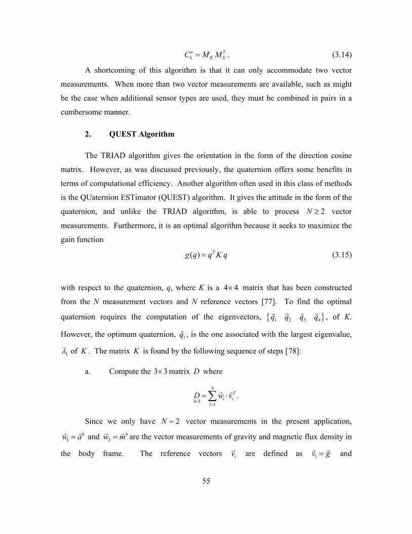
55

n Tb R SC M M . (3.14)

A shortcoming of this algorithm is that it can only accommodate two vector

measurements. When more than two vector measurements are available, such as might

be the case when additional sensor types are used, they must be combined in pairs in a

cumbersome manner.

2. QUEST Algorithm

The TRIAD algorithm gives the orientation in the form of the direction cosine

matrix. However, as was discussed previously, the quaternion offers some benefits in

terms of computational efficiency. Another algorithm often used in this class of methods

is the QUaternion ESTimator (QUEST) algorithm. It gives the attitude in the form of the

quaternion, and unlike the TRIAD algorithm, is able to process 2N vector

measurements. Furthermore, it is an optimal algorithm because it seeks to maximize the

gain function

( ) Tg q q K q (3.15)

with respect to the quaternion, q, where K is a 4 4 matrix that has been constructed

from the N measurement vectors and N reference vectors [77]. To find the optimal

quaternion requires the computation of the eigenvectors, 1 2 3 4q q q q

, of K.

However, the optimum quaternion, 1q

, is the one associated with the largest eigenvalue,

1 of K . The matrix K is found by the following sequence of steps [78]:

a. Compute the 3 3 matrix D where

3 3

1

.N

Ti i

i

D w v

Since we only have 2N vector measurements in the present application,

1bw a

and 2

bw m

are the vector measurements of gravity and magnetic flux density in

the body frame. The reference vectors iv

are defined as 1v g

and

56

2 cos 0 sinT

e ev B B

in the navigation frame, where eB

is the magnitude of

the earth’s magnetic flux density and is the local angle of inclination.

b. Construct the matrix TS D D

c. TZ D D

d. Obtain the vector z

from the elements of the skew symmetric matrix

Z such that

32 13 21 .z z z z

e. ( )trace D .

f. Construct the 4 4 matrix K ,

3 13 3

4 41 3 1 1

T

S I zK

z

.

The QUEST algorithm proceeds with the finding of the eigenvalues and eigenvectors of

K . Interestingly, as noted in the reference, for the special case 2N , the optimum

quaternion, 1q

is equivalent to the attitude matrix, nbC , which results from the TRIAD

algorithm.

3. FQA Algorithm

More recently, an alternative to the TRIAD and QUEST algorithm was

introduced. The Factored Quaternion Algorithm (FQA), while not optimal, provides

some attractive features. For one, unlike the TRIAD, the FQA produces a quaternion.

Another feature of the FQA is that it uses magnetic vector measurements only for the

computation of the yaw angle. Any errors present in this measurement are not coupled

into the roll and pitch angles [79]. Furthermore, the FQA was shown to give similar

57

performance to the QUEST at a reduced level of computational effort. It achieves this by

avoiding the use of trigonometric terms, which tend to increase the computational burden

of an algorithm.

The algorithm computes three distinct quaternions—each one corresponding to

the rotation about one of the principal axes. More to the point, the algorithm is rooted in

the fact that any orientation can be decomposed into an ordered set of rotations about the

principal axes of the reference (navigation) frame [80]. A final step of the FQA is to

multiply the three principal quaternions to yield a total or composite quaternion that

describes the complete three-dimensional orientation of the body as shown

.Yaw Pitch Rollq q q q (3.16)

The roll and pitch quaternions are computed form the acceleration vector measurement,

while the yaw quaternion is computed from the magnetic field vector measurement.

Given the normalized gravity vector measurement, , ,b b b bx y za a a a

where

1ba

, the pitch quaternion has the form

2

2

cos

0

sin

0

Pitchq

(3.17)

where

2

2

sin (sin ) 1 cos 2

cos 1 cos 2

sgn (3.18)

and

2

sin

cos 1 sin .

bxa

(3.19)

58

It is noted that in the equations provided above, the sine or cosine of the angle is

never actually computed. Beginning with the value for sin , it is carried through the

remaining expressions until the two half-angle terms are populated in the elements of the

pitch quaternion. In this manner, the FQA achieves a reduction in the amount of

numerical computations.

The roll quaternion is computed in a similar manner, but it accounts for any

rotation in the pitch angle. This quaternion has the form

2

2

cos

sin

0

0

Rollq

(3.20)

where

2

2

sin (sin ) 1 cos 2

cos 1 cos 2

sgn (3.21)

and

sin cos

cos cos .

by

bz

a

a

(3.22)

Next, the FQA computes the yaw quaternion using the magnetic field

measurement. First in this part of the computation is to determine the horizontal

components of the magnetic field vector measurement. This is done using the previously

computed pitch and roll quaternions

n b

Pitch Roll Roll Pitchm q q m q q

(3.23)

where nm

and bm

are expressed in the form of pure quaternions, that is

0n n n nx y zm m m m

and 0b b b b

x y zm m m m

. After normalization of the

resulting vectors, the yaw angle, , is related to the horizontal components of the

59

magnetic reference vector, x yN N , and the corresponding components of the

magnetic measurement vector, x yM M by

cos

sinx y x

y x y

M M N

M M N

. (3.24)

In the above equation, 1 0x yN N and 2 2n n n nx y x y x yM M m m m m .

Lastly, the yaw quaternion is given by

2

2

cos

0

0

sin

Yawq

. (3.25)

In a fashion similar to the roll and pitch quaternions, cos and sin are related to the

elements of the yaw quaternion through the half-angle formulas used previously.

The FQA uses vector measurements from the accelerometers and magnetometers.

The TRIAD and QUEST algorithms would use these same vector measurements, if they

were to be used in this application. Because of this, these algorithms require accurate

measurements from these sensors. For the magnetometers, it is widely understood that

errors can be introduced into the corresponding measurements due to magnetic

disturbances. Examples include electric machinery and electronics which generate their

own magnetic fields and add to the earth’s magnetic field. This type of interference is

known as hard-iron interference. Other examples include metallic objects, which do not

generate magnetic fields but can cause local variations in the magnetic field. Not

surprisingly, this is referred to as soft-iron interference [81]. As mentioned earlier, an

attractive feature of the FQA is that it isolates these unknown and unpredictable errors

from the pitch and roll angle computations.

In the absence of magnetic field interference and under static (or quasi-static)

conditions the FQA will produce an accurate attitude quaternion. However, if the sensor

60

body is accelerated, then the accelerometers will measure this acceleration in addition to

the component of the gravity vector. This latter component of the acceleration

measurement corresponds to the desired body orientation, but the former contributes an

unknown error into the FQA and to the resulting attitude quaternion.

C. QUATERNION-BASED COMPLEMENTARY FILTER

In the previous sections, several examples of algorithms were presented for the

computation of attitude. These algorithms were classified into two categories: those that

were based on angular rate measurements, which involved the solution of a dynamic

differential equation, and those that were based on angular measurements relative to two

or more reference axes.

In the present section, an alternative solution is presented, one that incorporated

both types of algorithms in the form of a complementary filter. As will be shown in the

remainder of this chapter, this architecture combined the attributes of both types of

algorithms, which in turn, helped to mitigate the inferior performance of the MEMS-

based IMMU.

Our proposed complementary filter had the architecture shown in Figure 25. The

filter blended a quaternion computed with the FQA (static branch) and another that was

computed using the angular rates (dynamic branch). The filter gain, k, had the effect of

adjusting the weight of either branch that was used in the final computation of a given

quaternion estimate, ˆ( )q t . During each iteration of the filter loop, an error, e(t), was

computed, which was the difference between the most recent quaternion computed with

the FQA, ( )sq t , and the estimate, ˆ( )q t , that had been computed during the previous filter

loop iteration. In the dynamic branch, a quaternion rate, ( )dq t , was computed from the

angular rates and combined with the error. The resulting differential equation was solved

numerically to yield the most recent estimate of ˆ( )q t . More details on the operation of

the filter will be presented in the following subsections.

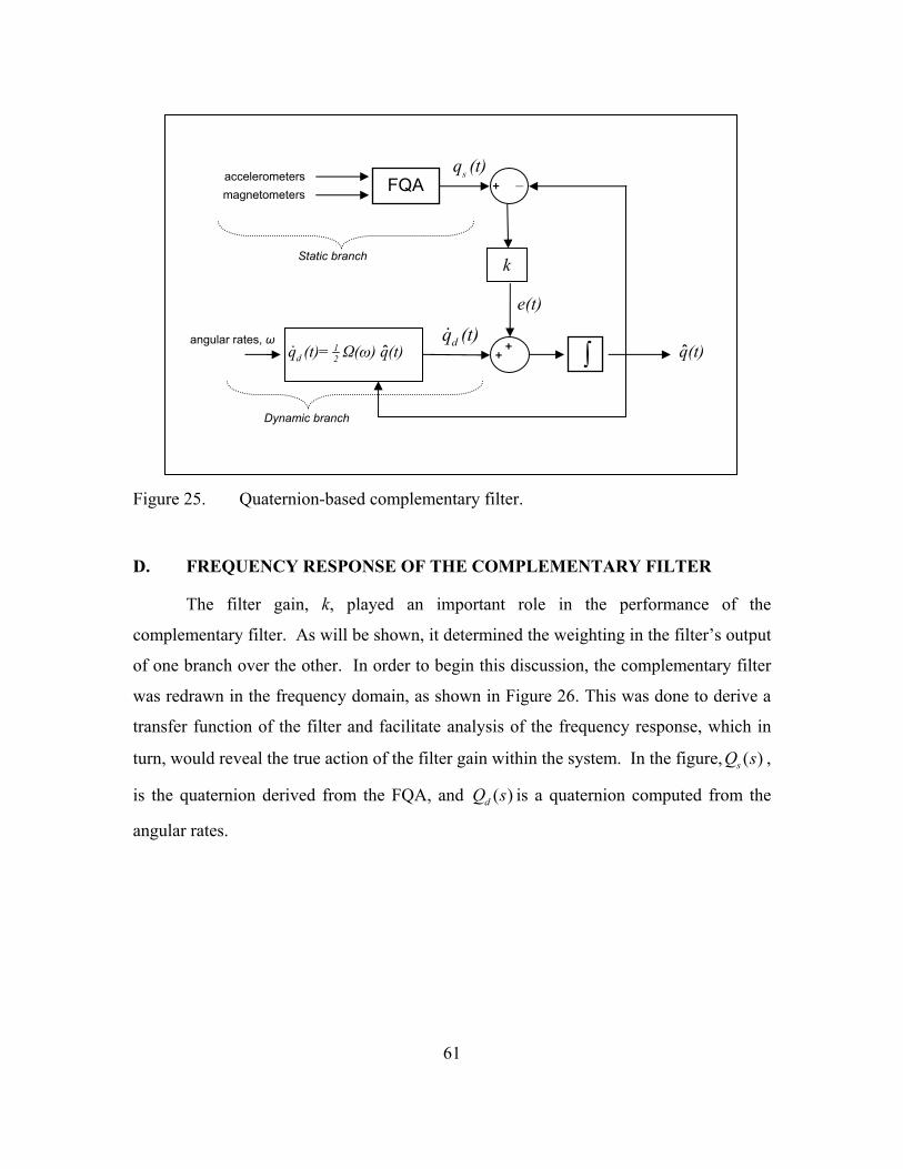
61

Figure 25. Quaternion-based complementary filter.

D. FREQUENCY RESPONSE OF THE COMPLEMENTARY FILTER

The filter gain, k, played an important role in the performance of the

complementary filter. As will be shown, it determined the weighting in the filter’s output

of one branch over the other. In order to begin this discussion, the complementary filter

was redrawn in the frequency domain, as shown in Figure 26. This was done to derive a

transfer function of the filter and facilitate analysis of the frequency response, which in

turn, would reveal the true action of the filter gain within the system. In the figure, ( )sQ s ,

is the quaternion derived from the FQA, and ( )dQ s is a quaternion computed from the

angular rates.

angular rates, ω

k

FQA

1d 2q (t)= Ω(ω) q(t) ˆ

+ _ accelerometers

magnetometers

sq (t)

q(t)ˆdq (t)

Static branch

Dynamic branch

+ +

e(t)

62

Figure 26. Complementary filter in the frequency domain.

First, we seek to derive the transfer function for the static branch. Applying the

principle of superposition and neglecting the filter input from the dynamic branch, we get

expressions for E(s) and ˆ ( )Q s , as shown in (3.26) and (3.27)

ˆ( ) ( ) ( )sE s k Q s Q s (3.26)

1ˆ ( ) ( )Q s E ss

(3.27)

Substitution of (3.26) into (3.27) and rearranging terms yields the desired

transfer function for the static branch of the complementary filter

ˆ ( )

( )s

Q s k

Q s s k

(3.28)

In terms of the magnitude frequency response, ( )sM , and the phase frequency

response, ( )s , for the static branch we have that

k

+ _ s

Q (s)

Q(s)ˆd

sQ (s) + +

1

s

E(s)

63

2 2

ˆ ( )( )

( )ss

Q j kM

Q j k

(3.29)

1

1

ˆ ( )( ) ( ) 0 tan ( )

( )

tan ( )

ss

k

Q jk j k kQ j

(3.30)

Figure 27 and Figure 28 show ( )sM and ( )s for three different values of gain

(plotted in blue). The horizontal axis on these plots are in terms of frequency (rad/sec),

but can be thought of as the rate of change of the input orientation or true quaternion.

( )sM has a low-pass response, which suggests that as the rate of change of the input

orientation increases, the static branch would tend to attenuate this signal and not

reproduce the true desired orientation. Moreover, we also note that ( )s increases from

zero to 2 as the orientation rate of change increases. Thus, there exists a phase

difference of 2 between the input and output of the static branch at high input

frequency.

Turning our attention to the dynamic branch, we once again apply the

superposition principle, but this time we ignore the input, ( )sQ s . Expressions for E(s)

and ˆ ( )Q s are given by

ˆ( ) ( )E s kQ s (3.31)

1ˆ ( ) ( ( ) ( ))dQ s sQ s E ss

(3.32)

Substitution of (3.31) into (3.32) and rearranging terms produces the transfer

function for the dynamic branch of the complementary filter:

ˆ ( )

( )d

Q s s

Q s s k

(3.33)

64

The magnitude frequency response, ( )dM , and the phase frequency response,

( )d , for the dynamic branch are

2 2

ˆ ( )( )

( )dd

Q jM

Q j k

(3.34)

1

ˆ ( )( ) ( )

( )

tan ( )2

dd

k

Q jj j k

Q j

(3.35)

Figure 27 and Figure 28 show these responses for the dynamic branch for three

values of gain (shown in red). We see that the magnitude response, ( )dM , of the

dynamic branch has a high-pass response, which suggests that this branch would be

appropriate for tracking orientation in situations where the attitude tended to change

rapidly. The phase frequency response, ( )d , reinforces this idea about the ability to

track rapidly changing orientation because we see that the phase change approaches zero

as the input frequency increases.

65

10-3

10-2

10-1

100

101

-20

-10

0

Mag

nitu

de (

dB)

Magnitude Response for Complementary Filter

k = 0.01

10-3

10-2

10-1

100

101

-20

-10

0

Mag

nitu

de (

dB)

k = 0.1

10-3

10-2

10-1

100

101

-20

-10

0

Frequency (rad/sec)

Mag

nitu

de (

dB)

k = 1

Figure 27. Magnitude response of static branch (blue) and dynamic branch (red).

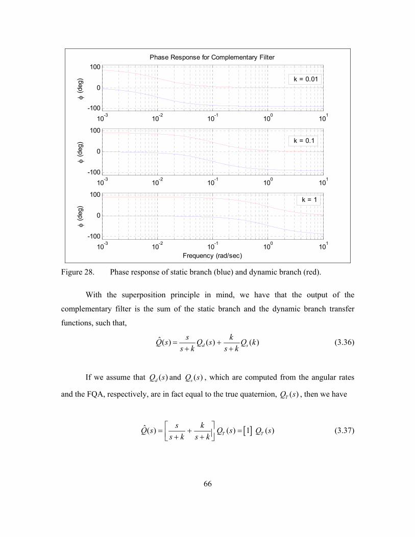
66

10-3

10-2

10-1

100

101

-100

0

100

(d

eg)

Phase Response for Complementary Filter

k = 0.01

10-3

10-2

10-1

100

101

-100

0

100

(d

eg) k = 0.1

10-3

10-2

10-1

100

101

-100

0

100

Frequency (rad/sec)

(d

eg)

k = 1

Figure 28. Phase response of static branch (blue) and dynamic branch (red).

With the superposition principle in mind, we have that the output of the

complementary filter is the sum of the static branch and the dynamic branch transfer

functions, such that,

ˆ ( ) ( ) ( )d s

s kQ s Q s Q k

s k s k

(3.36)

If we assume that ( )dQ s and ( )sQ s , which are computed from the angular rates

and the FQA, respectively, are in fact equal to the true quaternion, ( )TQ s , then we have

ˆ ( ) ( ) 1 ( )T T

s kQ s Q s Q s

s k s k

(3.37)

67

Therefore, our complementary filter has an overall transfer function of unity or an

all-pass response. There will not be any input frequency that is preferentially attenuated

in our complementary filter, and the phase of the output will be zero over all input

frequencies. These characteristics make the complementary filter suited to those

applications where a high-frequency measurement is to be blended with a low-frequency

measurement of the same process or physical quantity.

Before concluding this discussion on the frequency response of the

complementary filter, it is worthwhile to make one more examination of the frequency

response plots. Figure 27 shows the magnitude frequency response for k = 0.01, 0.1, and

1. From the plots we see that the gain is not only the corner frequency for the individual

branches in the complementary filter, but can also be thought of as a crossover frequency

for the filter—the point where the magnitude response in both branches are equal. The

plots serve to illustrate the concept that as the gain is increased, this crossover frequency

also increases. Consequently, the total output of our complementary filter has a

correspondingly larger portion derived from the static branch or ( )sQ s . Conversely, as

the filter gain is decreased, the output will be weighed more greatly by the quaternion

derived from the dynamic branch, ( )dQ s . In this fashion, the complementary filter can

be tuned to allow a greater or lesser amount of its output to be influenced by one branch

or the other.

E. ERROR ANALYSIS OF THE COMPLEMENTARY FILTER

With a preliminary understanding of the complementary filter and in preparation

for the filter performance analysis to be presented later, it is timely to consider the

relationship between the filter output and the sensor errors, which are certain to be found

within the accelerometers, magnetometers, and angular rate sensors. For this analysis,

the sensor errors are assumed to be small and constant over the time period of interest,

generally less than one second. These errors have a variety of sources including

variations in scaling coefficients over time, misalignment of the individual sensors, cross-

coupling between sensor axes, temperature dependence of the scaling coefficients, g-

dependent variations in gyro sensitivity, just to name a few of these factors.

68

1. Filter Performance Due to Gyro Error

The error analysis begins with the angular rate sensors. Measurements,

ˆ ˆ ˆ, ,xb yb zb , are expressed as the sum of the true angular rate, , ,xb yb zb , and the

sensor error, , ,xb yb zb as in

ˆ

ˆ

ˆ

xb xb xb

yb yb yb

zb zb zb

(3.38)

The dynamic three-dimensional attitude is derived from these measurements by

the differential equation

12

ˆˆ ˆ( ) ( ) ( )d dq t q t (3.39)

where ˆ( ) is the skew-symmetric matrix formed with the angular rate measurements

such that

ˆ ˆ ˆ0

ˆ ˆ ˆ0ˆ( )

ˆ ˆ ˆ0

ˆ ˆ ˆ 0

xb yb zb

xb zb yb

yb zb xb

zb yb xb

. (3.40)

Substituting (3.38) into (3.39), we have that

1 12 2

ˆ ˆ ˆ( ) ( ) ( ) ( ) ( )

( )d d d

d

q t q t q t

q t Q

(3.41)

The first term on the right hand side of (3.41) is the true dynamic rate quaternion that is

derived from the error-free component of the angular rate measurements. The second

term is a constant in the expression for the quaternion rate; it comes from the small

constant sensor error in the angular rate measurements. Next, assuming zero initial

conditions, we take the Laplace transform of (3.41) and have that

69

ˆ ( ) ( )d d

QsQ s sQ s

s

(3.42)

Referring to Figure 26 and deriving the transfer function for the complementary

filter output as was demonstrated in the previous section with (3.42) as an input, we have

that the filter output is

2ˆ ( ) ( ) ( )

1( ) ( )

d s

d s

Qs s k sQ s Q s Q s

s k s k s s k s

Qs kQ s Q s

s k s k s k s

(3.43)

If we have that ( )dQ s and ( )sQ s are equal to the true quaternion, then the filter output

becomes

1ˆ ( ) ( )T

QQ s Q s

s k s

(3.44)

The last term in (3.44) is the error in the filter output that is due to the small

constant error assumed in the angular rate measurements. Applying the inverse Laplace

transform to this term, we have that the error response in the complementary filter output

due to the errors in these measurements is

1 1( ) (1 )ktQ Q

error t es k s k

L (3.45)

This last result indicates that the error in the complementary filter output is related

to the constant error in the angular rate sensors, Q , and inversely proportional to the

filter gain. A non-zero gain will give an error that settles to a nominal value of

Q k after approximately five time constants or 5 / k seconds. Furthermore, as (3.45)

suggests, the error can be reduced by choosing k sufficiently large. However, as will be

explained in a later section, it is not a simple matter of making k large in the

70

complementary filter to control the effects of the angular rate measurement errors. When

k is large, the filter relies more greatly on the static quaternion, which in turn, is derived

from the accelerometer/magnetometer measurements. These sensors, not surprisingly,

come with their own set of errors that must be considered in some way.

Lastly, we consider the case when k = 0 in (3.45). In this situation, the

complementary filter output depends entirely on the angular rate measurements.

Expanding the exponential term with the Taylor series gives

2 3

2 3

1 1 12! 3!

2! 3!

kt kt ktQ Qe kt

k k

kt ktQkt

k

(3.46)

Neglecting the terms in (3.46) that have power 2 gives ( ) error t Q t (3.47)

This last result indicates that when k = 0 in the complementary filter, there will be a

linearly increasing error at the filter output due to the small angular rate sensor error.

2. Filter Performance Due to Accelerometer Error

Next, we turn our attention to the static quaternion that is derived from the FQA

and consider the impact of small constant errors in the accelerometers and magnetometers

of which there are three each. Within the FQA, the accelerometer measurements are used

to compute the pitch and roll angles of the orientation, while the magnetometers are used

to compute the yaw angle component. These angles are each cast into a quaternion form,

such that Yawq , Pitchq , and Rollq contain the yaw, pitch, and roll angles, respectively. A

final step in the FQA is to multiply these quaternions to give the complete orientation as

shown

s Yaw Pitch Rollq q q q (3.48)

71

To begin the analysis, it is assumed there is a small constant error in the xb–axis

accelerometer, such that

ˆb b bx x xa a a (3.49)

The remaining sensors are assumed free of any error in the ensuing analysis.

After [79], the pitch angle, is related to the xb–axis acceleration by

ˆˆ sinbxa (3.50)

Furthermore, we have that , and using the familiar trigonometric

identity sin( ) sin cos cos sinx y x y x y , (3.50) becomes

ˆ sin( )

sin cos cos sin

bxa

(3.51)

We expect that a small accelerometer error, bxa , will lead to small angular

error, . Additionally, when is small, cos 1 and sin , which simplifies

(3.51) to

ˆ sin cosbxa (3.52)

Lastly, taking (3.49) and (3.52) into consideration we have that

sinbxa (3.53)

cosbxa (3.54)

Eq. (3.53) simply states that the error-free part of the acceleration measurement

goes into computing the true pitch angle, while (3.54) relates the accelerometer error to

the resulting pitch angle error. With this understanding of how bxa introduces error into

72

the computed pitch angle, we seek to explore its impact on Pitchq and ultimately on the

static quaternion, sq . First, we write the pitch quaternion as

ˆ22

ˆ22

coscos

00ˆ

sinsin

00

Pitchq

(3.55)

Next, expanding cosine and sine terms with a first-order Taylor series, we have

that

2 2 2

2 2 2

cos sin

0 0ˆ

sin cos

0 0

Pitch

Pitch Pitch

q

q q

(3.56)

We recognize that the first quaternion in the right hand side of (3.56) is the true

pitch quaternion and that the second is an error quaternion that comes from the pitch

angle error, . Since we have in (3.54) that the is related to bxa , then we can infer

that Pitchq arises from the small accelerometer error that exists in ˆbxa .

The last step in this portion of the analysis is to establish how Pitchq manifests

itself in the static quaternion. Starting with (3.48) and substituting (3.56) into this

expression gives

ˆ ( )s Yaw Pitch Pitch Roll

Yaw Pitch Roll Yaw Pitch Roll

s s

q q q q q

q q q q q q

q Q

(3.57)

Eq. (3.57) shows that the output of the FQA is composed of the sum of a true

static quaternion, sq , and an error quaternion, sQ . This latter component is directly the

73

result of the small accelerometer error, bxa , introduced at the beginning of this analysis.

Since bxa was assumed to be a constant in this analysis, then sQ will also be a constant if

we make the additional assumption that there is no rotation in the roll and yaw angles.

Taking the Laplace transform of (3.57) we have that

ˆ ( ) ( ) ss s

QQ s Q s

s

(3.58)

Turning to the frequency domain representation of our complementary filter in

Figure 26, and applying (3.58) as an input to the filter, we have that the output of the

filter is now given by

ˆ ( ) ( ) ( ) sd s

Qs k kQ s Q s Q s

s k s k s k s

(3.59)

Once again as before, assuming that the ( )dQ s and ( )sQ s are equal to the true

quaternion, then the filter output becomes

ˆ ( ) ( ) sT

QkQ s Q s

s k s

(3.60)

The last term in (3.60) is recognized as the error in the quaternion output of the

complementary filter. Taking the inverse Laplace transform of this term gives the time-

domain representation of the error

( ) (1 )S

ktQ serror t Q e (3.61)

This result indicates that the error in the complementary filter output due to small

bxa settles to a steady-state value after approximately 5/k seconds. Furthermore, this

result differs from (3.45), which described the filter error in terms of the gyro error, ,

in that the magnitude of the error does not depend on the filter gain and therefore can not

be minimized or affected by a proper selection of k.

74

F. MATLAB IMPLEMENTATION

The complementary filter shown in Figure 25 represents the architecture of a filter

in continuous time. However, this filter can not be directly synthesized on a computer.

Instead, to permit analysis in MATLAB, the filter was programmed as shown in Figure

29. The filter loop began with an initial estimate of the quaternion, ˆ( 1)q n , which was

computed from the static acceleration and magnetometer measurements using the FQA.

For the initialization to be as accurate as possible, it was essential that ˆ( 1)q n be

computed when the subject was stationary. It was during those times when the FQA was

known to yield a reliable orientation estimate.

The algorithm then proceeded with the computation of a static quaternion, again

using the FQA. The next step in the iteration was to compute the error signal

incorporating the desired filter gain. The third step in the filter loop computed a dynamic

quaternion rate using the three-dimensional angular rate. The dynamic quaternion rate

and the error signal were then added in the subsequent step to produce another quaternion

rate, which was the rate of change of the quaternion we wish to estimate. Finally, using a

numerical integration technique, such as Euler’s method, the estimated quaternion was

derived. This result was then used to initialize the filter loop in a recursive fashion to

produce the next estimated quaternion.

75

Figure 29. Flow chart for MATLAB implementation of the complementary filter.

Begin Complementary

Filter ˆ( 1)q n

ˆ ˆ ˆ( ) ( )* ( ) ( 1)q n q n T n q n

( ) ( ( ), ( ))sq n fqa a n m n

1ˆ( ) ( ( ))* ( 1)

2dq n n q n

ˆ( ) * ( ) ( 1)se n k q n q n

ˆ ( ) ( ) ( )dq n e n q n

Use accelerometer, magnetometer measurements in FQA to get static quaternion

Apply filter gain, k

Use angular rates to get dynamic quaternion

Use Euler’s method to integrate previous result

Compute the estimate of the quaternion rate

76

G. A MODEL FOR PENDULUM MOTION SENSOR DATA

The previous section described how the complementary filter was programmed in

MATLAB. In the present section, we introduce a model of the vertical pendulum. The

purpose of this model was to generate data to aid in the study of the performance of the

complementary filter. In this synthetic pendulum, we consider a sensor module, like the

3DM-GX1 for example, to be attached at the swinging end. Expressions for the sensor

data were derived that described what the output of each sensor would be once the

pendulum was set into motion. In this manner, all of the real-world sensor artifacts, such

as gyro bias, accelerometer offset, and motion-induced acceleration, which undesirably

influenced the orientation estimate, could be controlled and examined in this simulated

experiment.

1. Pendulum Model for MATLAB Simulation

Figure 30 shows the pendulum with length, L; mass, m; viscous damping, c; and

angular displacement, . The coordinate system, b b bx y z , shown at A coincides with

the sensor body coordinate system, where the by axis is not shown because it is directed

orthogonal to the b bx z plane and projects inward into the plane of the paper. The axis

of rotation for the pendulum lies along the positive by axis, such that a positive rotation is

in the clockwise direction.

Summation of the forces acting at point A along the bx axis gives the dynamic

equation

sinbxF mL mg c (3.62)

Equation (3.62) is a non-linear second-order differential equation. An analytical solution

is not straightforward, but using one of MATLAB’s solvers for ordinary differential

equations, such as, ode45( ) for example, a numerical solution can be easily determined.

77

Figure 30. Pendulum model for MATLAB simulation.

With the parameters for our pendulum defined as L = 1 meter, g = 9.81 m/s2, m =

1 kg, c = 0.313 N·sec, and initial conditions (0) 10 , (0) 0 , the pendulum angle

with respect to time, along with the angular velocity and angular acceleration are shown

in Figure 31.

A

gravity

L

bx

bz

78

0 2 4 6 8 10 12 14 16 18 20-10

0

10

(d

eg)

Simulated Pendulum

0 2 4 6 8 10 12 14 16 18 20-50

0

50

' (

deg/

sec)

0 2 4 6 8 10 12 14 16 18 20-100

0

100

'' (

deg/

sec2 )

time (sec)

Figure 31. Pendulum motion with (0) 10 , L = 1 meter, g = 9.81 m/s2, m = 1 kg, and c = 0.313 N·sec.

2. Sensor Data Generated with the Pendulum Model

The previous section provided the pendulum’s angular displacement, velocity,

and acceleration. Next, we consider a sensor module, such as the 3DM-GX1, attached to

point A of the pendulum. Recall that the sensor module was equipped with three

accelerometers, three magnetometers, and three angular rate sensors. In this section, we

seek expressions that describe each of these sensor outputs when the module is stimulated

by the pendulum motion. Given these expressions for the sensor data outputs, we will

have a well understood set of data that can be used in the study of the complementary

filter.

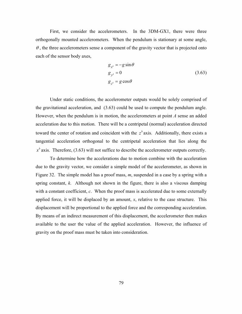
79

First, we consider the accelerometers. In the 3DM-GX1, there were three

orthogonally mounted accelerometers. When the pendulum is stationary at some angle,

, the three accelerometers sense a component of the gravity vector that is projected onto

each of the sensor body axes,

sin

0

cos

b

b

b

x

y

z

g g

g

g g

(3.63)

Under static conditions, the accelerometer outputs would be solely comprised of

the gravitational acceleration, and (3.63) could be used to compute the pendulum angle.

However, when the pendulum is in motion, the accelerometers at point A sense an added

acceleration due to this motion. There will be a centripetal (normal) acceleration directed

toward the center of rotation and coincident with the bz axis. Additionally, there exists a

tangential acceleration orthogonal to the centripetal acceleration that lies along the

bx axis. Therefore, (3.63) will not suffice to describe the accelerometer outputs correctly.

To determine how the accelerations due to motion combine with the acceleration

due to the gravity vector, we consider a simple model of the accelerometer, as shown in

Figure 32. The simple model has a proof mass, m, suspended in a case by a spring with a

spring constant, k. Although not shown in the figure, there is also a viscous damping

with a constant coefficient, c. When the proof mass is accelerated due to some externally

applied force, it will be displaced by an amount, x, relative to the case structure. This

displacement will be proportional to the applied force and the corresponding acceleration.

By means of an indirect measurement of this displacement, the accelerometer then makes

available to the user the value of the applied acceleration. However, the influence of

gravity on the proof mass must be taken into consideration.

80

Figure 32. Accelerometer model. (a) Simple mass and spring model, and (b) free body diagram of the accelerometer proof mass.

Figure 32 also shows the free body diagram of the proof mass suspended within

the accelerometer case and the following equation accounts for all the forces acting on

the proof mass:

x

F ma mg kx cx (3.64)

Dividing (3.64) by the proof mass, we have an expression in terms of the acceleration

k c

a g x xm m

(3.65)

Furthermore, we recognize that the accelerometer produces at its output a value that is

proportional to x, so we define f as the accelerometer output, and we have that

kf x

mk

f xm

(3.66)

m

k

x+

m

x+

cxkx

mg

(a) (b)

81

Substituting (3.66) into (3.65), we have an expression that gives the dynamic output of

the accelerometer in terms of the applied acceleration, a, and the gravity, g,

c

a g f fk

(3.67)

To conclude the analysis of the accelerometer, we take the Laplace transform of

(3.67) to get

( ) ( ) ( ) ( )c

A s G s F s sF sk

(3.68)

Rearranging (3.68), we have the accelerometer output as

( ) ( )

( )1 1c c

k k

A s G sF s

s s

(3.69)

Next, regarding the applied acceleration and the gravity as step inputs into the

accelerometer for t > 0 such that

1

1

( ) ( )

( ) ( )

A s a u t

G s g u t

L

L (3.70)

then, if we apply the Laplace final value theorem to (3.69), we have that

0 0( ) lim ( ) lim

1 1

gas s

c cs sk k

f sF s ss s

a g

(3.71)

Thus, we conclude that the accelerometer output is equal to the difference

between the applied acceleration and the gravity vector. For the case of the triad of

orthogonally-mounted accelerometers, (3.71) is tailored to the situation when only a

component of the gravity vector is aligned with the sensor body axis. Therefore, (3.71)

becomes the set of equations

82

b b b

b b b

b b b

y y y

z z z

x x xf a g

f a g

f a g

(3.72)

Finally, substituting (3.63) into (3.72) and accounting for the centripetal

acceleration and the tangential acceleration of the pendulum, we have the accelerometer

outputs given by

2

sin

0

cos

b

b

b

x

y

z

f L g

f

f L g

(3.73)

Eq. (3.73) provides the accelerometer outputs for the pendulum motion within the earth’s

gravity field. Conveniently, the accelerometer outputs are expressed in terms of the

pendulum angular displacement, angular velocity, and angular acceleration.

Next, we consider the three angular rate sensors. Since the pendulum was

constrained to swing in the b bx z plane, then only the angular rate sensor aligned with the

by axis would sense any rotation. The angular rate sensors oriented along the bx axis and

the bz axis would not sense the pendulum’s movement. Thus, we have that for the angular

rate sensors, their outputs would be as

0

0

b

b

b

x

y

z

(3.74)

83

Finally, we come to the magnetometers. These sensors measure the component of

the earth’s magnetic flux density that has been projected onto each of the sensor body

axes. To simplify this part of the pendulum model, we consider that the plane of motion

of the pendulum is aligned with magnetic north. Doing this simplifies the analysis of the

magnetometers. Figure 33 examines this aspect of the pendulum model. In the figure,

the earth referenced coordinate system is shown as n n nx y z . The vector, eB

, is the

earth’s magnetic flux density, which makes an angle, , with the nx axis; it is commonly

referred to as the angle of inclination. This vector is known to vary both in magnitude

and direction around the globe, however, for the local area, the values of eB

= 0.486 gauss

and = 60.483 degrees were noted from the National Oceanic and Atmospheric

Administration (NOAA) Web site. Finally, referring again to Figure 33, we derive the

following expressions for the magnetometer sensors:

cos( )

0

sin( )

b

b

b

e

e

x

y

z

m B

m

m B

(3.75)

84

Figure 33. Magnetic flux density vector relative to the sensor body axes ( b bx z ) and the navigation frame ( n nx z ).

With expressions for all nine sensors in hand, the next step was to generate

simulated pendulum motion data and insert this synthetic data into our complementary

filter. If the complementary filter was to work correctly, then the filter would produce

the pendulum motion as described by our simulation model.

A

eB

bx

bz

nz

nx

85

3. MATLAB Plots of Simulated Sensor Data

Given the expressions for the sensor outputs in (3.73), (3.74), and (3.75), the next

task was to use these equations to generate synthetic sensor data. A MATLAB script was

written that produced the synthetic sensor data set using these equations. A time

increment was chosen to give an approximate sampling rate of 50 samples per second—

similar to that provided by the 3DM-GX1. The script produced an array of incremental

time and sensor data samples; it then saved the array in a data file called SimData.mat.

The format of the data file was similar to that which was normally generated using the

actual 3DM-GX1 sensor, except that the quaternion was not included here. Each row in

the array corresponded to a sample time and the relevant sensor data from that sample

time instant. The accelerometer sensor data was computed with (3.73) as shown in

Figure 34. Figure 35 shows the angular rate sensor data that was derived from (3.74).

Lastly, Figure 36 shows the magnetometer data generated with (3.75).

0 2 4 6 8 10 12 14 16 18 20-0.02

0

0.02

a x (G

)

Acceleration

0 2 4 6 8 10 12 14 16 18 20-1

0

1

a y (G

)

0 2 4 6 8 10 12 14 16 18 20-1.05

-1

-0.95

a z (G

)

time (sec)

Figure 34. Simulated accelerometer data from the pendulum model.

86

0 2 4 6 8 10 12 14 16 18 20-1

0

1

x (

deg/

sec)

Angular Rate

0 2 4 6 8 10 12 14 16 18 20-50

0

50

y (

deg/

sec)

0 2 4 6 8 10 12 14 16 18 20-1

0

1

z (

deg/

sec)

time (sec)

Figure 35. Simulated angular rate data from the pendulum model.

87

0 2 4 6 8 10 12 14 16 18 200.1

0.2

0.3

mx (

gaus

s)

Magnetic Flux Density

0 2 4 6 8 10 12 14 16 18 20-1

0

1

my (

gaus

s)

0 2 4 6 8 10 12 14 16 18 200.35

0.4

0.45

0.5

mz (

gaus

s)

time (sec)

Figure 36. Simulated magnetometer data from the pendulum model.

88

H. COMPLEMENTARY FILTER STUDY WITH SIMULATED PENDULUM

Leading up to this point, we have modeled the sensor outputs of the 3DM-GX1

attached to point A of the vertical pendulum. With the corresponding sensor data now

available, we were able to begin a study of the performance of the complementary filter.

The filter algorithm was programmed in MATLAB as shown in Figure 29. To begin

iteration of the filter, we required an initial value for ˆ(0)q and to set the filter gain, k, to

some desired value. Using the FQA, ˆ(0)q was computed using (0) (0) (0)b b bx y zf f f and

(0) (0) (0)b b bx y zm mm , which were derived with (3.73) and (3.75). For 0k , the

complementary filter only weighs the angular rate measurements in its output, neglecting

( )sq t that was derived from the FQA. This was considered a good starting place to begin

looking at the filter performance. Figure 37 shows the output of the complementary filter

for the case 0k . It shows the individual elements of the quaternion, ˆ( )q t . However,

since the performance of the filter is difficult to interpret by inspection of the quaternion,

ˆ( )q t was converted into equivalent Euler angles and the result plotted in Figure 38.

89

0 5 10 15 200.996

0.997

0.998

0.999

1

1.001Quaternions

q0

0 5 10 15 20-1

-0.5

0

0.5

1

q1

0 5 10 15 20-0.1

-0.05

0

0.05

0.1

q2

Time (sec)0 5 10 15 20

-1

-0.5

0

0.5

1

q3

Time (sec)

Figure 37. Complementary filter output for k = 0.

90

0 2 4 6 8 10 12 14 16 18 20-1

0

1

Rol

l (de

g)

Euler Angles

0 2 4 6 8 10 12 14 16 18 20

-10

0

10

Pitc

h (d

eg)

0 2 4 6 8 10 12 14 16 18 20-1

0

1

Yaw

(de

g)

Time (sec)

C.F. true

Figure 38. Complementary filter output (red) shown in Euler angles, k = 0. True pendulum angle (blue). No difference between true angle and computed angle.

Figure 38 shows that the complementary filter (red) with 0k accurately tracks

the true pendulum angle (blue) as given by the simulation model. Since there was no

difference between the true pendulum angle and that computed by the complementary

filter, the curves are shown superimposed in the pitch plot. The computed pitch angle

reproduced all of the features of the true pendulum motion from the initial value of

10 deg to the end of the simulation period. The complementary filter also computed

zero for the roll and yaw angles because there was no movement in those axes.

This example assumed ideal angular rate sensors that did not have any noise or

bias in their output. In practice, however, all angular rate sensors possess some amount

of error in sensitivity and bias. Therefore, to examine these types of sensor errors, we

introduce a small bias error into the angular rate sensors. Microstrain specified in their

documentation a 0.033% bias error for the 3DM-GX1. This value was used to create a

new set of pendulum sensor data as described in the previous section. The

91

complementary filter algorithm was repeated using the new sensor data to produce the

pendulum angles shown in Figure 39. This figure reveals the effect of the small bias

error on the computed angles when k = 0. The pitch angle tracked the true angle during

the first few cycles, but began to drift away from the true track towards the end of the

motion period. Where the roll and yaw angles were zero in the previous example, they

now exhibited an error that grew without bound. This result is consistent with the error

predicted in (3.47). With k = 0, the error due to the small angular rate sensor error is

unbounded. However, if the filter gain were to be increased, then the error is expected to

be contained to within some constant value. The next example explores this idea in more

detail.

0 2 4 6 8 10 12 14 16 18 200

1

2

3

Rol

l (de

g)

Euler Angles

0 2 4 6 8 10 12 14 16 18 20

-10

0

10

Pitc

h (d

eg)

0 2 4 6 8 10 12 14 16 18 200

1

2

3

Yaw

(de

g)

Time (sec)

C.F. true

Figure 39. Complementary filter output with small bias error in angular rate sensors and k = 0.

92

Next, we consider the performance of the complementary filter due to the FQA.

For this example, the gain will be set to a value that weighs the static branch more greatly

than the dynamic branch. Figure 40 shows the magnitude frequency response for k = 50.

With this particular gain value programmed in the complementary filter, the pendulum

angle, which has a radian frequency of 3.128 rad/sec, is computed mainly from the FQA.

At this frequency, the dynamic branch is attenuated by more than 20 dB. Thus, its

contribution to the filter output is suppressed more than 100 times than that of the static

branch.

10-3

10-2

10-1

100

101

102

103

-20

-15

-10

-5

0

Mag

nitu

de (

dB)

Magnitude Response

k = 50

Figure 40. Magnitude response of the complementary filter with k = 50. Static branch (blue), dynamic branch (red).

93

Using this gain value, the complementary filter output is examined in Figure 41.

The roll and yaw angles show a small error on the order of 0.002 degrees. This is the

result of the small bias error introduced into the angular rate sensors. Furthermore, it is

noted that the error does not seem to grow in time as it does in Figure 39. But instead,

the error remains constant throughout the period of the pendulum motion, as indicated by

(3.45). Lastly, the figure also shows the pitch angle of the pendulum. Examination of

this plot shows that the complementary filter (red) is not able to track the true pendulum

angle (blue). However, this is not due to the filter algorithm, but is an artifact of the

accelerometer measurements which not only sense the acceleration due to gravity, but

also have the response due to the centripetal and tangential acceleration, see (3.73).

0 2 4 6 8 10 12 14 16 18 200

2

4x 10

-3

Rol

l (de

g)

Euler Angles

0 2 4 6 8 10 12 14 16 18 20-10

0

10

Pitc

h (d

eg)

0 2 4 6 8 10 12 14 16 18 200

2

4x 10

-3

Yaw

(de

g)

Time (sec)

C.F. true

Figure 41. Filter output (red) with k = 50. True pendulum angle (blue).

94

To explore this last notion in greater detail, the simulated pendulum data was

generated once again, however the centripetal acceleration and tangential acceleration

were omitted from the expressions for the accelerometer output, see (3.73). With this

new data provided to the complementary filter, Figure 42 shows that the static branch

does give an accurate orientation when it is given accelerometer measurements that are

comprised only of acceleration due to the sensed gravity vector. As seen in the figure,

the true pendulum angle (blue) and the complementary filter angle (red) are

superimposed in the pitch angle plot. Interestingly, the roll angle shows a small

oscillation where none had existed previously. This is explained by considering the

tangential acceleration. Coincidentally, it oscillates in a similar fashion, but with an

opposite phase. When both components of acceleration are accounted for, as they are in

Figure 41, the oscillation cancels and only the error due to the gyro bias persists.

0 2 4 6 8 10 12 14 16 18 200

2

4x 10

-3

Rol

l (de

g)

Euler Angles

0 2 4 6 8 10 12 14 16 18 20-10

0

10

Pitc

h (d

eg)

0 2 4 6 8 10 12 14 16 18 200

2

4x 10

-3

Yaw

(de

g)

Time (sec)

C.F. true

Figure 42. Filter output (red) with k = 50. Tangential and centripetal acceleration omitted from accelerometer measurements. True pendulum angle (blue).

95

Figure 42 illustrated that the source of angular error in the FQA is due to non-

gravitational accelerations. Practically speaking, however, the accelerometers respond to

any and all acceleration and are not capable of discriminating between those accelerations

due to the changing orientation and those arising from linear or rotational accelerations.

Thus, if the accelerometers are to be a part of the orientation sensing solution, some

means of mitigating the error in ( )sq t that arises because of the non-gravitational

accelerations must be identified.

Continuing our study of the complementary filter performance, the situation for

pendulum motion with large damping is investigated. Here, the viscous damping is

increased to 5.95 N·sec to produce the pendulum motion shown in Figure 43. Comparing

this with the pendulum motion shown in Figure 31, which was the case for viscous

damping equal to 0.313 N·sec, we see that the pendulum moves much more slowly and

does not oscillate about the vertical. Next, the simulated sensor data is applied to the

complementary filter with k = 50. The complementary filter output is shown in Figure

44. Recall that this value of gain caused the filter to weigh ( )sq t more greatly than ( )dq t ,

as seen in Figure 40. The accelerometers have a response due to gravity, as well as, the

centripetal and tangential accelerations. However, since these latter accelerations are

smaller because of the pendulum’s retarded motion, the accelerometer outputs have a

larger component due to the sensed gravity vector. This in turn improves the filter’s

overall ability to determine the pendulum angle. The pitch angle error is less than two

degrees at t = 1 sec, and decreases to less than 0.2 deg at t = 2 sec. The error in the roll

and yaw angles was due to the small bias error introduced earlier into the angular rate

measurements. Furthermore, we note that the error does not grow in time, but remains

constant as shown in the figure.

96

0 2 4 6 8 10 12 14 16 18 20-10

0

10

(d

eg)

Simulated Pendulum

0 2 4 6 8 10 12 14 16 18 20-20

-10

0

10

' (

deg/

sec)

0 2 4 6 8 10 12 14 16 18 20-100

-50

0

50

'' (

deg/

sec2 )

time (sec)

Figure 43. Pendulum motion with viscous damping, c = 5.95 N·sec.

97

0 2 4 6 8 10 12 14 16 18 200

2

4x 10

-3

Rol

l (de

g)

Euler Angles

0 2 4 6 8 10 12 14 16 18 20-10

0

10

Pitc

h (d

eg)

0 2 4 6 8 10 12 14 16 18 200

2

4x 10

-3

Yaw

(de

g)

Time (sec)

C.F. true

Figure 44. Complementary filter output (red) with k = 50. True pendulum angle (blue).

Up to this point, we have examined the complementary filter with filter gain

0k and 50k . To conclude our study of the complementary filter performance using

the simulated pendulum, the pendulum simulation was conducted once more, but this

time the filter gain will be set to a nominal value of 1k . This value was selected

without regard to optimizing the performance of the filter, but rather to examine the

performance at some intermediate value of filter gain. The pendulum viscous damping

is set to c = 0.313 N·sec, which gives the pendulum motion shown previously in Figure

31. With this value of gain, the resulting filter performance is shown in Figure 45. The

roll and yaw angles have a constant error (after the transient response) on the order of 0.1

degrees, which is due to the gyro bias error that was included in the simulation. The

pitch angle error is at most 1 degree, but appears to track better than the case when

98

50k . An effort to optimize the error was not made here, as this will be done later, but

this exercise serves to illustrate the need for tuning of the filter gain to give desirable

performance.

0 2 4 6 8 10 12 14 16 18 200

0.1

0.2

Rol

l (de

g)

Euler Angles

0 2 4 6 8 10 12 14 16 18 20

-10

0

10

Pitc

h (d

eg)

0 2 4 6 8 10 12 14 16 18 200

0.1

0.2

Yaw

(de

g)

Time (sec)

C.F. true

Figure 45. Complementary filter output (red) with k = 1. True pendulum angle (blue).

Summarizing, the performance of the complementary filter algorithm depends in

large part on the value of gain, k, used within the filter. A small k will place a greater

weight on ( )dq t , so the filter output has a larger part derived from the angular rate

sensors. The ability of the filter to track the pendulum motion when this was the case

was shown to be adequate during the initial period of the pendulum motion; however, any

small bias errors in the angular rate sensor data results in an angle error that grows with

time. From this observation, we make the general statement that the filter gives

99

acceptable results with small k when it is utilized over a small period of time—before the

error has grown beyond an acceptable level. Furthermore, we note that when the

pendulum motion contained relatively large centripetal and tangential acceleration, a

large k did not yield good angle tracking performance. But, a large k will give acceptable

filter results when the pendulum motion was low with small centripetal and tangential

acceleration, as was the case with large viscous damping. For this case, the filter tracked

the pendulum angle after a brief transient period, and in the steady state it was able to

maintain a small error. Additionally, the large k produced an output angle error that was

constant and did not grow with time. Moving forward, the challenge for the application

of the complementary filter is to identify a suitable value for k.

I. FILTER PERFORMANCE WITH REAL PENDULUM DATA

The previous section described the performance of the complementary filter using

simulated data. The selection of the gain, k, was discussed with regard to its effect on the

ability of the filter to track the pendulum angle. In this section, we examine the

complementary filter using real sensor data from the 3DM-GX1. The performance is

compared against the pendulum angle measured with a 16-bit shaft encoder. To collect

the data from the real pendulum, a LabView program was developed that ran on a Dell

Latitude D620 laptop computer. It read the raw counts from the 16-bit shaft encoder, as

well as, the sensor data from the 3DM-GX1 attached to point A. Figure 46 shows a block

diagram of the data acquisition system. The LabView program controlled the operation

of the National Instruments USB-6501, which provided the necessary interface for the

eleven control/data lines of the A58 encoder. Additionally, the program read the sensor

data from the 3DM-GX1 through the laptop’s RS-232 serial communications port. All

the data was arranged into a time-stamped array, which was written to a data file on the

computer hard drive. Later, the data file was imported into MATLAB for processing and

analysis.

100

Figure 46. Data acquisition system developed for the vertical pendulum.

The vertical pendulum provided a good platform to investigate the

complementary filter performance. It was easy to change the length of the pendulum to

yield different natural frequencies, and the amplitude of oscillation could be made to

vary, as well. Numerous trials were conducted in the laboratory with the vertical

pendulum and the 3DM-GX1. Figure 47 shows the complementary filter output with the

pendulum length adjusted to 1 meter and the filter gain, k, set to 0.15. The computed

pitch angle (red) appears to follow the angle measured with the A58 encoder (blue) to

within two degrees. The roll and yaw angles exhibit an error of similar magnitude. The

blue lines shown in the roll and yaw plots coincide with the initial computed angles; it is

not an indication of an encoder measurement along those axes. The roll and yaw plots,

however, show some computed motion in these angles. Since the data acquisition system

does not provide a means for measurement of motion in these angles, it can not be

concluded with certainty that the angular error observed in the computed roll and yaw

angles is wholly due to the complementary filter algorithm. The pendulum shaft is made

of a wooden dowel and may exhibit some twisting and flexing when in motion.

Secondly, because no means for precise alignment of the sensor body axes with the

11 DIO Lines

RS-232

USB

National Instruments USB-6501

Microstrain 3DM-GX1

x

z

A

A58 Rotary Shaft Encoder

Dell Latitude D620

101

pendulum axes was available, the motion observed in the roll and yaw axes may in fact

be due to a small pendulum alignment error. Therefore, some of the angular motion

observed in these plots may be accurate. On the other hand, the 3DM-GX1, as well as,

many other sensors of this type, possesses some degree of cross-coupling error. This

error produces a sensor output in an axis normal to the axis of motion and is the result of

the sensor axes not being completely orthogonal. Overall, the computed angles are on the

order of two degrees from the expected angles and are certainly within the dynamic

accuracy specified by the manufacturer for their own proprietary quaternion algorithm.

0 10 20 30 40 50 60 70 80-3

-2

-1

0

Rol

l (de

g)

Euler Angles

0 10 20 30 40 50 60 70 80-20

0

20

Pitc

h (d

eg)

0 10 20 30 40 50 60 70 8042

43

44

45

Yaw

(de

g)

Time (sec)

C.F. Encoder

Figure 47. Computed angles (red) vs. expected angles (blue) of the vertical pendulum, k = 0.15.

Figure 48 and Figure 49 compare the pendulum angles computed by the

complementary filter with those acquired directly from the 3DM-GX1. The pitch angle,

shown in Figure 48, indicates that the Microstrain algorithm is more accurate in this

particular case since the angle is shown to be within 0.5 degrees of the encoder-measured

angle. Figure 49 is similar to Figure 47, but it includes the angles derived from the

102

Microstrain algorithm. Comparing the roll angle computed by Microstrain’s algorithm

and that from our complementary filter, we note that they have similar behavior. The

yaw angles differ somewhat, however, they both are within two degrees of the expected

angle shown in blue. Finally, comparing the pitch angle, shown in the center of the plot,

indicates that our complementary filter performs similarly to Microstrain’s algorithm

over the entire interval of motion.

20 25 30 35 40 45

-15

-10

-5

0

5

10

Time (seconds)

Ang

le (

degr

ees)

Encoder

Comp Filter

Microstrain

Figure 48. Pendulum pitch angle: Complementary filter with k = 0.15 (red), 16-bit Encoder (blue), and Microstrain’s proprietary algorithm (green).

103

0 10 20 30 40 50 60 70 80-4

-2

0

Rol

l (de

g)

Euler Angles

0 10 20 30 40 50 60 70 80-20

0

20

Pitc

h (d

eg)

0 10 20 30 40 50 60 70 8042

43

44

45

Yaw

(de

g)

Time (sec)

C.F. Encoder Microstrain

Figure 49. Pendulum pitch angle: Complementary filter with k = 0.15 (red), 16-bit Encoder (blue), and Microstrain’s proprietary algorithm (green).

Before leaving this section, the question arises as to what would be a reasonable

value to use for the filter gain, k. The plots in Figure 47, Figure 48, and Figure 49 were

all generated with our complementary filter having k = 0.15. In order to arrive at this

value, several trials of the pendulum were conducted. The data from these trials were

then processed with a MATLAB script that varied the range of k from 0 to 1. For each

trial, the MATLAB script computed the total root mean square (RMS) angle error over

the entire period of motion. Figure 50 shows the RMS angle error for each trial.

The plot shows that when 0k , we have a large angle error. For this gain, the

filter uses the gyro measurements exclusively, and the bias errors of these sensors are the

source of the corresponding angular error. As the gain is increased from zero, then the

angle error decreases, as predicted by (3.45); however, it begins to increase after the gain

exceeds approximately 0.15. This is caused by the fact that more of the filter output is

weighed by the FQA as the gain is increased. Recall that the FQA relies on the

accelerometer measurements, which in turn measure the centripetal/tangential

104

accelerations of the pendulum, as well as, the component of the gravity vector. As a

result, the FQA introduces an ever increasing error into the filter output as the gain is

increased beyond 0.15. Therefore, for the plots shown previously, k = 0.15 was chosen

for use in our complementary filter.

0 0.1 0.2 0.3 0.4 0.5 0.6 0.7 0.8 0.9 10.5

1

1.5

2

2.5

3

3.5

4

4.5

5

Filter Gain, k

RM

S E

rror

(de

g)

trial 1

trial 2

trial 3

trial 4

Figure 50. Selection of filter gain using real pendulum motion data.

This section discussed the performance of the complementary filter using data

that was collected from a vertical pendulum. The performance of the complementary

filter was compared with the angle measured by a 16-bit rotary encoder attached to the

pendulum shaft. For the filter gain of k = 0.15, the performance of the complementary

filter was found to be comparable to that reported by Microstrain’s proprietary filter and

also demonstrated an ability to track the true angle to within 2 degrees.

105

J. FILTER PERFORMANCE WITH RANDOM MOTION

The last chapter ended with a description of the anomalous drift observed in the

Microstrain-computed quaternion. It showed how the angle was prone to drift for a

substantial amount of time (on the order of 20 seconds or more) when the sensor was

subjected to an energetic random motion. In the present section, this motion will be

supplied to our complementary filter so that its performance can be assessed with this

same type of stimulus. When the sensor body was subjected to the arbitrary motion that

resulted in the drifting angle, all of the sensor data (i.e., accelerometers, magnetometers,

and angular rates) were recorded to file. Subsequently, these data were available for

testing with our complementary filter.

Figure 51 compares the manufacturer’s quaternion with that derived from our

complementary filter using k = 0.15 supplied with the sensor data collected from that

experiment. Before the motion, t < 15 sec, the manufacturer’s quaternion and that from

our filter tend to agree. This is the time period when the sensor body is resting

motionless on the workbench. During the motion interval, 15 < t < 20 sec, it is not

possible to make a comparison since we do not have a means of measuring the true

orientation. Therefore, we make no statement about the filter performance during this

interval. However, after the motion stops, and the sensor is returned onto the workbench

in its original orientation, we observe that the components of the quaternion from our

complementary filter tend to settle more quickly to their original values. Figure 52

makes the same comparison in terms of the Euler angles computed from the respective

quaternion. It further illustrates how our complementary filter tends to perform better

than the manufacturer’s quaternion in this situation when the motion is erratic or

changing abruptly.

106

0 20 40 600.85

0.9

0.95

1

q0

Quaternions

Motion

0 20 40 60-0.2

-0.1

0

0.1

0.2

q1

Motion

0 20 40 60

-0.2

0

0.2

q2

seconds

Motion

0 20 40 60-0.4

-0.2

0

0.2

0.4

0.6

q3

seconds

Motion

Figure 51. Comparison of Microstrain quaternion (blue) and that from our complementary filter with k = 0.15 (red).

107

0 10 20 30 40 50 60

-20

0

20

Rol

l (de

g)

Euler Angles

Motion

0 10 20 30 40 50 60

-20

0

20

Pitc

h (d

eg)

Motion

0 10 20 30 40 50 60-20

0

20

40

60

Yaw

(de

g)

Time (seconds)

Motion

Figure 52. Comparison of Microstrain Euler angles (blue) and those derived from our complementary filter with k = 0.15 (red).

Lastly, in Figure 53, we explore the idea of switching the filter gain to an alternate

value based on some criterion that was monitored during the execution of the algorithm.

The figure shows the same data from Figure 52, but it also includes the result of this gain

switching strategy. In this approach, the filter algorithm switched the gain to a large

value, relatively speaking, when the motion was considered low. This had the effect of

weighing the accelerometers and magnetometers more greatly in the complementary filter

output when the acceleration due to non-gravitational motion was low. To accomplish

this adaptive gain strategy, the angular rate was monitored during the program iteration,

and when it was observed to be below a particular threshold, the gain was raised to k = 1.

When the motion was considered to be above the threshold, as established by the angular

rate, the gain was then returned to k = 0.15. The figure shows this result for the period

after t = 15 sec, as this was considered to be the more interesting interval of motion.

After the motion stopped, the angles derived from the adaptive gain approach settled

more quickly than those derived from the constant gain filter. During that period, t > 20

108

sec, the sensor was resting on the workbench, which provided an opportunity to use the

accelerometers/magnetometers for the orientation computation. Because the sensor body

was stationary, the accelerometers were not influenced by any motion and their response

was due entirely to the gravity vector. At the end of the motion, however, both

techniques appeared to yield similar results.

15 20 25 30 35 40 45 50 55 60

-20

0

20

Rol

l (de

g)

Euler Angles

Motion

15 20 25 30 35 40 45 50 55 60

-20

0

20

Pitc

h (d

eg)

Motion

15 20 25 30 35 40 45 50 55 60-20

0

20

40

60

Yaw

(de

g)

Time (seconds)

Motion

Figure 53. Comparison of results in Figure 51 and the adaptive gain complementary filter (green).

K. SUMMARY

This chapter presented the complementary filter and discussed its performance in

terms of the gain. A vertical pendulum served as the test case for an evaluation of the

filter’s performance. In closing this chapter, it is noted that the adaptive-gain

complementary filter appears to give slightly better results than the constant-gain filter

without too much added complexity. The next chapter considers the adaptive gain filter

in the personal navigation application. As will be shown, the adaptive gain

109

complementary filter is ideally suited to this problem. During the course of natural

human walking, the motion of the foot is observed to be composed of a swing phase and

a stance phase with abrupt starts and stops dividing these periods of motion. It is during

these periods that the complementary filter gain can be adaptively switched to take

advantage of this natural part of normal walking. Thus, during the stance phase, the gain

can be set to some nominally high value to affect full use of the accelerometers (and

magnetometers) for sensing orientation. Similarly, during the swing phase, the gain can

be set to a low value so that the filter will utilize the angular rate sensors as much as

possible to give the attitude estimate.

110


111

IV. PERSONAL NAVIGATION

The previous chapter introduced the complementary filter for use in estimating

the attitude quaternion. It blended a “static” quaternion from the FQA with a “dynamic”

quaternion that came from a differential equation involving the gyro measurements. In

addition to a constant gain, the previous chapter also presented the idea of adaptively

switching the filter gain based on some parameter that is monitored during the execution

of the algorithm.

In this chapter, the complementary filter is applied to the strapdown navigation

algorithm for use in computing one’s position in a PNS application. A foot motion model

is also developed here. It will be used to carry out a simulation study of the PNS

algorithm and to examine some of its other relevant aspects, such as the selection of the

numerical integration method used in the strapdown portion of the algorithm and the

sensor sampling interval. In addition to the simulation, some example results of the PNS

algorithm using actual data will also be included at the end of this chapter.

A. STRAPDOWN ALGORITHM FOR PERSONAL NAVIGATION

The strapdown navigation algorithm with the zero-velocity updates, the gait-phase

detection algorithm, and our quaternion complementary filter is shown in the block

diagram in Figure 54. The inputs to this algorithm are the IMMU sensor measurements

from the accelerometers, magnetometers, and gyros. A timer value is required, which is

also provided by the IMMU microcontroller. The output of the algorithm is np

, a

3 1 vector of computed position in the navigation frame. Dashed lines from the gait-

phase detection block indicate that this function controls the operation of the zero-

velocity updates and the complementary filter. Recall that the zero-velocity updates were

employed to correct the error that had accumulated in nv

. This feature was applied when

the foot was known to have a zero velocity during the stance phase. For the

complementary filter, the gait-phase detection algorithm served to indicate the

appropriate times to adaptively switch the filter gain.

112

Figure 54. Strapdown navigation algorithm with zero-velocity updates, gait-phase detection, and quaternion–based complementary filter.

B. ANALYSIS OF NUMERICAL METHODS FOR THE PNS

With a technique in hand for the computation of one’s position using the foot-

mounted IMMU, it might be an appropriate time to test this algorithm with some actual

foot motion data. However, this will be deferred until the end of the chapter. Instead, in

this section we explore the remaining components within the PNS algorithm (see Fig. 54)

that may require some additional examination, namely the integrators. For example,

within the complementary filter, there is an integration operation that results in the need

to solve a first-order differential equation during each iteration of the PNS algorithm.

The differential equation is of the form

1.

2q t q t (4.1)

In Chapter III, which dealt with the analysis and performance of this filter, this

equation was solved with the numerical method known as Euler’s method. In the

strapdown navigation portion of the PNS, two additional integrators can be found. The

first integrator serves to generate velocity data from the derived samples of navigation

( )bqL aba

na

+

g

_

nv

np

0nv

0

np

ZUPT

12( ) ( ) ˆ( )dq t q t

( )sq t

( )q t

( )dq t

e(t)

+ _

+ +

b

bm

ba

FQA

k

Gait-Phase Detection

.

113

frame acceleration, while the second integrator provides the desired position updates.

The resulting integral equations have the form as shown.

( ) ( )

( ) ( ) .

v t a t dt

p t v t dt

(4.2)

Not surprisingly, some numerical integration method must be employed here, as

well. Solution of these integral equations requires numerical methods known as Newton-

Cotes formulas [82]. The idea behind these methods is to approximate the sampled data

with a polynomial that is easy to integrate. Euler’s method considers a zero-order

polynomial and gives a numerical formula—for example, written to compute velocity—

that is of the form

1 .k k kv v t a

(4.3)

This method is easy to implement in code and requires only one data sample. To

improve the accuracy of the result, another popular method for numerical integration is

known as the Trapezoidal Rule. It considers a first-order polynomial as an approximation

for the sampled data and generally yields superior results to Euler’s method. It has the

convenient form

1 1

1.

2k k k kv v t a a

(4.4)

It requires two data samples, but this is generally not a limitation. Depending on

the underlying nature of the data samples and the requirements for accuracy, higher-order

numerical methods, such as Simpsons 1/3 and 3/8 rules, may be considered for a given

application [83]. In general, the higher-order methods give more accurate results at the

expense of more computational effort. Another factor affecting the accuracy is the size

of the sampling interval, t . This parameter is the interval of time between samples, and

it is often cited in terms of the sampling frequency, 1sf t . Ordinarily, the accuracy

of the solution improves as t decreases.

114

The main objective of this section is to explore the various methods available for

numerical integration with regard to their application in the PNS. Specifically, we are

concerned with the two integrators in the strapdown portion of the PNS, that is, those

dealing with the computation of velocity and position. The reason we will not explore

the integrator residing in the complementary filter is that this performance has already

bees studied in Chapter III. A second objective of this section will be to determine a

maximum sampling interval, t .

Before proceeding too much further into the analysis of the integrators, it is

essential to establish a performance benchmark. This is some known quantity or result

that we can use to compare the performance of the various numerical methods that will

be considered, as well as, their sensitivity to the sampling frequency.

1. Benchmark Selection Criteria

A simple benchmark might be to use the actual walking data and try different

numerical methods to see which one gives the minimum distance error. While this may

be the benchmark we return to at the end of this analysis, we prefer to use a carefully

selected acceleration model for the ensuing analysis. This approach has validity for the

following reasons:

1) An acceleration model allows the variation of the sampling frequency, sf ,

either up or down. With actual data, we can only down-sample the data, and only by

fixed amounts (i.e. 2sf , 3sf , 4sf , …).

2) The analysis can be carried out in the absence of sensor noise and calibration

errors. When appropriate, this parameter can be introduced as desired to study its effect

on the overall performance.

3) An acceleration model, unlike real measured acceleration data, provides a

known and well understood reference for the performance study. This begs the question,

“What is an appropriate model for foot acceleration to use in this analysis?”

To help answer this question, consider the foot acceleration from one of the

navigation frame coordinate axes shown in Figure 55. It is real data derived from the

115

foot-mounted IMMU during normal walking motion. Acceleration from approximately

24 steps were superimposed on the plot to show the behavior of the foot motion during

the swing phase. From the moment the toe leaves the ground at the end of the stance

phase, the curve peaks rapidly with some positive acceleration then quickly changes sign

as the foot slows down in preparation for the end of the swing phase when the heel strikes

the ground.

0 0.1 0.2 0.3 0.4 0.5 0.6 0.7 0.8 0.9 1-40

-30

-20

-10

0

10

20

30

40

50Foot Acceleration - Nav Coordinates

Time (sec)

Acc

eler

atio

n (m

/s2 )

Figure 55. Typical foot acceleration in navigation coordinates, 24 steps shown.

Integration of this data, using the Trapezoidal rule, for example, gives the velocity

profile shown in Figure 56. Consistent with our intuition, the plot shows how the foot

velocity increases at the beginning of the swing phase, then decreases returning to zero as

it should for the stance phase. It is also noted that these curves have the correction

116

introduced by the zero-velocity updates. Lastly, one more integration, again by the

Trapezoidal rule, gives the foot displacement in this particular navigation frame

coordinate axis, as shown in Figure 57.

0 0.1 0.2 0.3 0.4 0.5 0.6 0.7 0.8 0.9 1-0.5

0

0.5

1

1.5

2

2.5

3

3.5

4

4.5Foot Velocity - Nav Coordinates

Time (sec)

Vel

ocity

(m

/s)

Figure 56. Typical foot velocity in navigation coordinates.

117

0 0.1 0.2 0.3 0.4 0.5 0.6 0.7 0.8 0.9 1-0.2

0

0.2

0.4

0.6

0.8

1

1.2

1.4Foot Position - Nav Coordinates

Time (sec)

Pos

ition

(m

)

Figure 57. Typical foot displacement in navigation frame coordinates.

In choosing an acceleration model for our analysis, we desire it to have the

behavior depicted in the previous figures for the real foot motion. That is, for the

acceleration, there should be a period of zero acceleration that corresponds to the stance

phase. There should also be a period of acceleration corresponding to the swing phase.

The swing phase acceleration will have an interval of positive acceleration followed by a

period of negative acceleration. Upon integration of the acceleration model, the result

should appear similar to the curves depicting the foot velocity, as shown in Figure 56. At

the end of the acceleration period, the velocity curve should be zero. Finally, for the

position, we would like to see that the resulting displacement has a shape similar to that

shown in Figure 57.

118

2. Linear Acceleration Model

A simple model that was initially considered approximated the swing phase

acceleration with a linear polynomial. This model is given as

3 2

( ) 12 6 , 0s sL La t t t

(4.5)

where sL is the foot displacement, and is the duration of the swing phase. This

polynomial is applied to a model of the foot acceleration that is comprised of a period of

zero acceleration representing the stance phase and the linear acceleration during the

swing phase, with another 0.1 seconds of zero acceleration representing the heel strike

event at the end of the foot swing. This is better illustrated in Figure 58 where the

acceleration model includes the linear polynomial ( )a t given in Eq. (4.5). The figure also

shows a computed velocity and displacement, both of which were computed using the

Trapezoidal rule. Foot displacement, sL , was assumed equal to 180 cm, = 400 msec,

and sf =1000 Hz.

In Table 4, the velocity error (in cm) and the position error (in %) are given for

several sampling frequencies ranging from 20 Hz to 1000 Hz. The velocity error, as

expected, is small due to the fact that the polynomial approximation provided by the

Trapezoidal rule is exact for the case of the linear acceleration model. On the other hand,

the position error that we observe at the end of the swing phase clearly shows a

dependence on sf . A criticism of this simple linear model pertains to the discontinuity

that exists in the acceleration profile at 0.5 sec and 0.9 sec, marking the beginning and

end of the swing phase. Natural human motion can not produce acceleration profiles

having such discontinuities.

119

0 0.1 0.2 0.3 0.4 0.5 0.6 0.7 0.8 0.9 1-1

0

1x 10

4

a(t)

cm

/s2

Polynomial Acceleration Model

0 0.1 0.2 0.3 0.4 0.5 0.6 0.7 0.8 0.9 10

500

1000

v(t)

cm

/s

0 0.1 0.2 0.3 0.4 0.5 0.6 0.7 0.8 0.9 10

100

200

s(t)

cm

Time (sec)

Figure 58. Linear polynomial acceleration model for one step.

Table 4. Position error performance for linear acceleration model and varying sampling frequency.

sf (Hz) sT (sec) Velocity Error

(cm/sec)

Position Error (%)

20 0.05 131.705 10 40.15

50 0.02 0 15.47

100 0.01 147.105 10 7.622

200 0.005 141.421 10 3.781

500 0.002 132.789 10 1.505

1000 0.001 143.73 10 0.7512

120

3. Sinusoidal Acceleration Model

Another model that was given ample consideration was that of a sinusoid. Here

the acceleration in the swing phase had the expression

( ) cos , 0 .2

sL ta t t

(4.6)

Using this expression in the model for the foot acceleration, we get the plot in Figure 59,

again as before, with sL = 180 cm, = 400 msec, and sf =1000 Hz. Table 5 shows the

dependence of the error to the sampling frequency using the Trapezoidal rule for

integration. We also see that the velocity error performance is much worse than that for

the linear model. This is due to the fact that our acceleration model is not linear, and the

polynomial approximation provided by the trapezoidal rule is no longer exact. The

acceleration curve still has the discontinuity at the beginning and end of the swing phase.

In experimentation with this model, it was also learned that this feature introduced an

undesirable sensitivity to the distribution of the data samples. Slightly shifting the data

samples forwards or backwards in time caused large swings in the resulting error. For

this reason, as well as the discontinuities in the curve, this model was abandoned and not

considered further in this analysis.

121

0 0.1 0.2 0.3 0.4 0.5 0.6 0.7 0.8 0.9 1-1

0

1x 10

4

a(t)

cm

/s2

Sinusoidal Acceleration Model

0 0.1 0.2 0.3 0.4 0.5 0.6 0.7 0.8 0.9 10

500

1000

v(t)

cm

/s

0 0.1 0.2 0.3 0.4 0.5 0.6 0.7 0.8 0.9 10

100

200

s(t)

cm

Time (sec)

Figure 59. Sinusoidal acceleration model for one step.

Table 5. Position error performance for sinusoidal acceleration model and varying sampling frequency.


(cm/sec)

Position Error (%)

20 0.05 277.6 47.56

50 0.02 111 18.71

100 0.01 55.52 9.304

200 0.005 27.76 4.639

500 0.002 11.1 1.853

1000 0.001 5.552 0.9257

122

4. Gaussian Acceleration Model

The Gaussian (normal) function occurs often in the modeling of natural

phenomenon. It was also considered here as a model for the swing phase acceleration. In

our adaptation of this function, the swing phase velocity had the form of the familiar

Gaussian function as shown

2 221

( ) , 2 22t

sv t L e t

(4.7)

where =0.05 was found by trial and error to give a curve that looked like the velocity

profile derived from the actual data, and sL is the stride length. Using ( )v t as shown in

Eq. (4.7), the acceleration can be easily derived

2 22

2

( )( ) .

2tsLd v t t

a t edt

(4.8)

Figure 60 shows this expression applied to the foot motion acceleration. Immediately it

can be seen that this model does not have a discontinuity as large as that exhibited by the

models considered previously. However, there is some minor abrupt change at the start

and end of the swing phase due to the fact that the exponential function is not identically

zero at these points. In spite of this, the model does show superior performance as

indicated in Table 6. These results were computed using the Trapezoidal rule.

123

0 0.1 0.2 0.3 0.4 0.5 0.6 0.7 0.8 0.9 1-2

0

2x 10

4

a(t)

cm

/s2

Gaussian Acceleration Model

0 0.1 0.2 0.3 0.4 0.5 0.6 0.7 0.8 0.9 10

500

1000

1500

v(t)

cm

/s

0 0.1 0.2 0.3 0.4 0.5 0.6 0.7 0.8 0.9 10

100

200

s(t)

cm

Time (sec)

Figure 60. Gaussian acceleration model for one step.

Table 6. Position error performance for the Gaussian acceleration model and varying sampling frequency.


(cm/sec)

Position Error (%)

20 0.05 132.253 10 -0.04155

50 0.02 136.122 10 -0.04978

100 0.01 136.908 10 -0.07585

200 0.005 138.377 10 -0.09327

500 0.002 132.419 10 -0.105

1000 0.001 131.793 10 -0.1092

124

Next, we consider the performance of several numerical integration methods. Up

to this point, we have only utilized the Trapezoidal rule for integration. In the following

analysis, we will also employ Euler’s method, Simpson’s 1/3 rule, and an adaptation of

Simpson’s rule and Trapezoidal rule referred to here as modified Simpson’s 1/3 rule. It

works to preserve the sampling interval of the resulting data so that the number of

samples available for a subsequent integration is maintained. These results are shown

qualitatively in the following graphs.

Figure 61 shows the position derived from the double integration of the Gaussian

acceleration model with sf =100 Hz. The true position, which was derived analytically

using MATLAB’s erfc( ) function, is shown in blue. The symbols in the plot are the

results from the various integration methods considered. Red dots are used to identify the

result using MATLAB’s cumtrapz( ) function, which accomplished the Trapezoidal rule

for integration. The author also implemented his own function for the Trapezoidal rule

titled myTrapz( ). This was done to facilitate its use in other functions used here, such as

Simpson’s 1/3 and the modified Simpson’s 1/3 rules. As evidenced by the plot, the

results from myTrapZ( ) agree with those of MATLAB’s cumtrapz( ), thus validating its

use in the higher-order functions. The plot also shows the results from the double

integration of the Gaussian acceleration model using Simpson’s 1/3 rule, modified

Simpson’s 1/3 rule, and Euler’s method. As the figure suggests, for this sampling

frequency, all methods utilized here gave acceptable results for this particular

acceleration model.

125

0 0.1 0.2 0.3 0.4 0.5 0.6 0.7 0.8 0.9 10

20

40

60

80

100

120

140

160

180

Position fs = 100 Hz

Time (sec)

s(t)

cm

TruecumTrapZ

myTrapZ

Simpsons 1/3

Modified SimpsonsEuler

Figure 61. Double integration of Gaussian acceleration model, sf = 100 Hz.

The experiment was repeated using a reduced sampling frequency of sf =50 Hz.

This result is shown in Figure 62. For this sampling frequency, all methods perform well.

Euler’s method begins to degrade, however, during the intermediate portion of the

integration interval, but at the end, its result is consistent with those derived from the

higher-order methods. Lastly, the experiment was repeated one more time, but with

sf =20 Hz. As shown in Figure 63, at the end of the integration period, the Trapezoidal

rule, along with Euler’s method, appears to give better results. Simpson’s 1/3 rule and

the modified Simpson’s rule, on the other hand, appear to have degraded performance for

this sampling frequency. This may be due to the fact that while these higher-order

methods generally yield better results, in this particular case, for the limited number of

samples available, the second-order approximation utilized by these methods may tend to

exacerbate the error.

126

0 0.1 0.2 0.3 0.4 0.5 0.6 0.7 0.8 0.9 10

20

40

60

80

100

120

140

160

180

Position fs = 50 Hz

Time (sec)

s(t)

cm

TruecumTrapZ

myTrapZ

Simpsons 1/3



127

0 0.1 0.2 0.3 0.4 0.5 0.6 0.7 0.8 0.9 10

20

40

60

80

100

120

140

160

180

200

Position fs = 20 Hz

Time (sec)

s(t)

cm

TruecumTrapZ

myTrapZ

Simpsons 1/3



5. Bezier Polynomial Acceleration Model

One last model we wish to consider is derived from a well known family of

functions known as Bezier polynomials. An attractive feature of these polynomials is

that they can be tailored to suit a particular application. Yet another benefit is that

analytical expressions for integrals and derivatives can be easily derived. Here, the

polynomial chosen has a signature that is representative of the position,

5 4 35 4 3

6 15 10( ) , 0 .ss t L t t t t

(4.9)

The acceleration is easily derived from the second derivative of ( ).s t

128

2

3 22 5 4 3

( ) 120 180 60( ) .s

d s ta t L t t t

dt

(4.10)

This acceleration model does not have a discontinuity of any kind at the beginning and

end points of the modeled interval, as demonstrated by the fact that (0) ( ) 0a a .

Figure 64 shows the foot model acceleration incorporating this particular Bezier

polynomial. Table 7 has the results from the variation of the sampling frequency with the

Trapezoidal rule integration.

0 0.1 0.2 0.3 0.4 0.5 0.6 0.7 0.8 0.9 1-1

0

1x 10

4

a(t)

cm

/s2

Bezier Polynomial Acceleration Model

0 0.1 0.2 0.3 0.4 0.5 0.6 0.7 0.8 0.9 1-500

0

500

1000

v(t)

cm

/s

0 0.1 0.2 0.3 0.4 0.5 0.6 0.7 0.8 0.9 10

100

200

s(t)

cm

Time (sec)

Figure 64. Bezier polynomial acceleration model.

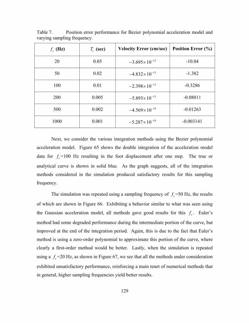
129

Table 7. Position error performance for Bezier polynomial acceleration model and varying sampling frequency.

sf (Hz) sT (sec) Velocity Error (cm/sec) Position Error (%)

20 0.05 133.695 10 -10.04

50 0.02 134.832 10 -1.382

100 0.01 132.398 10 -0.3286

200 0.005 135.893 10 -0.08011

500 0.002 144.569 10 -0.01263

1000 0.001 145.287 10 -0.003141

Next, we consider the various integration methods using the Bezier polynomial

acceleration model. Figure 65 shows the double integration of the acceleration model

data for sf =100 Hz resulting in the foot displacement after one step. The true or

analytical curve is shown in solid blue. As the graph suggests, all of the integration

methods considered in the simulation produced satisfactory results for this sampling

frequency.

The simulation was repeated using a sampling frequency of sf =50 Hz, the results

of which are shown in Figure 66. Exhibiting a behavior similar to what was seen using

the Gaussian acceleration model, all methods gave good results for this sf . Euler’s

method had some degraded performance during the intermediate portion of the curve, but

improved at the end of the integration period. Again, this is due to the fact that Euler’s

method is using a zero-order polynomial to approximate this portion of the curve, where

clearly a first-order method would be better. Lastly, when the simulation is repeated

using a sf =20 Hz, as shown in Figure 67, we see that all the methods under consideration

exhibited unsatisfactory performance, reinforcing a main tenet of numerical methods that

in general, higher sampling frequencies yield better results.

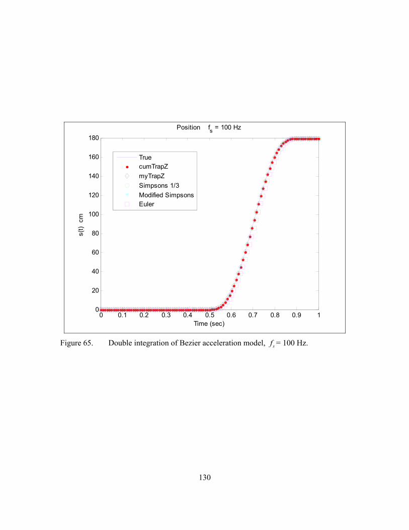
130

0 0.1 0.2 0.3 0.4 0.5 0.6 0.7 0.8 0.9 10

20

40

60

80

100

120

140

160

180

Position fs = 100 Hz

Time (sec)

s(t)

cm

TruecumTrapZ

myTrapZ

Simpsons 1/3


Figure 65. Double integration of Bezier acceleration model, sf = 100 Hz.

131

0 0.1 0.2 0.3 0.4 0.5 0.6 0.7 0.8 0.9 10

20

40

60

80

100

120

140

160

180

200

Position fs = 50 Hz

Time (sec)

s(t)

cm

TruecumTrapZ

myTrapZ

Simpsons 1/3



132

0 0.1 0.2 0.3 0.4 0.5 0.6 0.7 0.8 0.9 10

20

40

60

80

100

120

140

160

180

Position fs = 20 Hz

Time (sec)

s(t)

cm

TruecumTrapZ

myTrapZ

Simpsons 1/3



6. Summary of Numerical Methods

To summarize the previous discussion concerning the performance study of the

various numerical methods and the sampling frequency, we learned several things. First,

the acceleration model used in the study does have an impact on the resulting error. As

we observed early on when we experimented with the sinusoidal acceleration model,

large errors had surfaced after double integration. Upon further study, we concluded that

the discontinuous features of our model made the numerical method sensitive to these

errors. Those models that did not have large discontinuities did not exhibit this behavior.

Another aspect of the performance of the numerical methods we considered

pertains to the manner in which the data samples were distributed over the interval of

integration. Slightly shifting the sample points forwards or backwards in time also

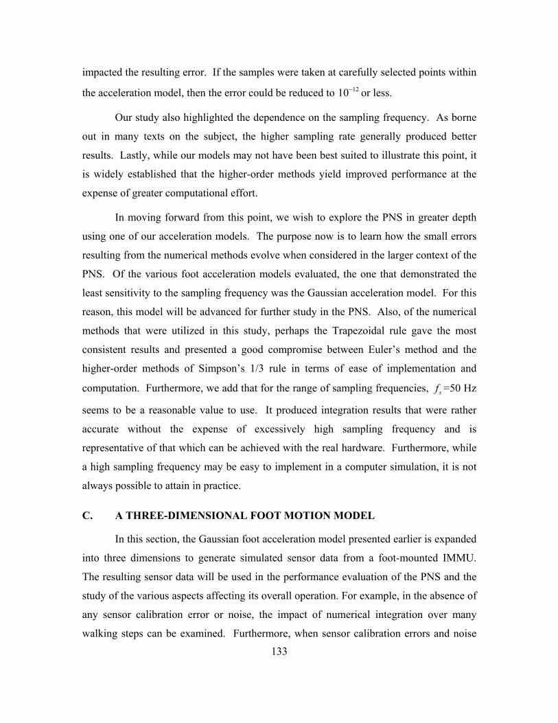
133

impacted the resulting error. If the samples were taken at carefully selected points within

the acceleration model, then the error could be reduced to 1210 or less.

Our study also highlighted the dependence on the sampling frequency. As borne

out in many texts on the subject, the higher sampling rate generally produced better

results. Lastly, while our models may not have been best suited to illustrate this point, it

is widely established that the higher-order methods yield improved performance at the

expense of greater computational effort.

In moving forward from this point, we wish to explore the PNS in greater depth

using one of our acceleration models. The purpose now is to learn how the small errors

resulting from the numerical methods evolve when considered in the larger context of the

PNS. Of the various foot acceleration models evaluated, the one that demonstrated the

least sensitivity to the sampling frequency was the Gaussian acceleration model. For this

reason, this model will be advanced for further study in the PNS. Also, of the numerical

methods that were utilized in this study, perhaps the Trapezoidal rule gave the most

consistent results and presented a good compromise between Euler’s method and the

higher-order methods of Simpson’s 1/3 rule in terms of ease of implementation and

computation. Furthermore, we add that for the range of sampling frequencies, sf =50 Hz

seems to be a reasonable value to use. It produced integration results that were rather

accurate without the expense of excessively high sampling frequency and is

representative of that which can be achieved with the real hardware. Furthermore, while

a high sampling frequency may be easy to implement in a computer simulation, it is not

always possible to attain in practice.

C. A THREE-DIMENSIONAL FOOT MOTION MODEL

In this section, the Gaussian foot acceleration model presented earlier is expanded

into three dimensions to generate simulated sensor data from a foot-mounted IMMU.

The resulting sensor data will be used in the performance evaluation of the PNS and the

study of the various aspects affecting its overall operation. For example, in the absence of

any sensor calibration error or noise, the impact of numerical integration over many

walking steps can be examined. Furthermore, when sensor calibration errors and noise

134

are ultimately incorporated into the model, an assessment of their effect can be

ascertained, as well. Varying amounts of these variables can be included to gain greater

insight into the sensitivity of the PNS with respect to these parameters. To develop our

foot motion model, our approach is to first generate simulated sensor data of a foot-

mounted IMMU for one step, then propagate this model over as many steps as desired for

use in stimulating the PNS.

In Figure 68, the navigation reference frame along with a body reference frame

attached to the foot center-of-mass is shown. For our motion model, the foot has been

constrained to rotate only about the ny -axis described by the pitch angle . This angle

represents the natural rotation exhibited by the foot as it moves between the swing and

stance phase. Translation or displacement of the foot is confined to the n nx z plane.

Therefore, in our simulation, the accumulated distance traveled in the horizontal direction

corresponds to magnetic North and coincides with the nx -axis. Our model also has an

acceleration along the nz -axis to represent the vertical movement of the foot, but its net

displacement is zero at the end of each step, as it should during normal walking on level

ground. No acceleration occurs along the ny -axis; thus, the net displacement in the

easterly (or westerly) direction is zero.

Figure 68. Reference frames for the foot motion model.

yb

xb

zb

xn

znyn

135

The movement of the foot during one step can be decomposed into four distinct

motions. Until now, the motion of the foot was considered only in terms of a stance

phase and a swing phase, but for added realism, the stance phase will be broken down

into three parts. Table 8 shows this new classification of the foot motion. For simplicity,

the total duration for one step is assumed equal to one second. The foot motion model

begins with the foot-flat phase; its duration is 0.4 seconds. In this phase, there is no

angular rotation of the foot here, nor is there any acceleration. The next period of the

model has the toe-off phase, which lasts 0.1 seconds. There is no translational motion

during this phase, but there is a rotation with the heel lifting off the ground in preparation

for the swing phase. Next, there is the swing phase in which the acceleration will be

derived from a Gaussian model, as described shortly. Duration of this phase is 0.4

seconds and has a positive angular rate, as shown in the table. Lastly, the heel-strike

phase occurs at the end of the swing phase. The acceleration here has returned to zero

when the heel of the foot strikes the ground and the foot pitch angle rotates back to zero

to coincide with the beginning of a new foot-flat phase.

Table 8. Component phases of one walking step.

Acceleration

Phase

Duration

(seconds)

Angular Rate

(rad/sec) xA zA

Foot-flat 0.4 0 0 0

Toe-off 0.1 -7.5 0 0

Swing 0.4 +3.5 Gaussian Gaussian

Heel-strike 0.1 -6.5 0 0

To make the sensor data for one step of foot motion, the task is broken down into

four separate parts. First, quaternions are constructed from the foot pitch angle. This

angle is easily derived from the angular rate that has been assumed for each phase of the

foot motion, as shown in the table above. These quaternions have the form

136

cos2

0.

sin2

0

q

(4.11)

Secondly, after the quaternions have been established for all four phases of the

model, they are then used to rotate the navigation frame acceleration into the body frame,

as shown in Figure 69. Unlike the quaternion rotation operator used in the strapdown

navigation algorithm, the rotation operator used here works with the conjugate

quaternion, q , as shown. A description of the navigation frame acceleration is given in

the next sub-section.

Figure 69. Method to generate body frame acceleration from navigation frame acceleration.

The third step in this process is to use the pitch angle to construct the

magnetometer measurements. This set of expressions takes on the same form as that

used in Chapter III for the pendulum motion simulation, where eB

= 0.486 gauss and =

60.483 degrees,

cos( )

0

sin( )

b

b

b

ex

y

ez

m B

m

m B

(4.12)

( )n

qL a

bana

g

+

q

137

The fourth and final step of this process is to construct the gyro measurements.

This is straightforward using the data in Table 8. Since rotation is confined to the ny -

axis, which is coincident with the by -axis, only the corresponding gyro measures any

rotation. The gyro measurement designated as by is equal to depending on the

particular phase of the foot motion, and the remaining two gyros do not sense any

rotation, as shown below:

0

0.

b

b

b

x

y

z

(4.13)

1. Three-Dimensional Acceleration Model

The previous section showed how to construct the sensor body gyro and

magnetometer measurements. To construct the sensor body acceleration measurements,

ba

, the method illustrated in Figure 69 must be employed. However, this requires that

first the navigation frame accelerations, na

, be established. Fortunately, this is

straightforward because the foot motion in this frame is rather intuitive. As stated

previously, the accelerated motion has been constrained to lie in the n nx z plane, with

the foot pitch rotation required to occur along the ny -axis. Furthermore, this leads to the

convenient fact that the b bx z plane is parallel to the n nx z plane. Therefore,

accelerations occurring in the n nx z plane reside wholly in the b bx z plane, and no

acceleration exists along the ny -axis nor in the by -axis.

For the nxa acceleration, we note that the velocity in the navigation frame should

have a shape that is similar to the bell-shaped curve in Figure 56. Recall that this was the

computed velocity of the foot in navigation-frame coordinates. For this component of the

velocity, we adopt the Gaussian function, as before,

138

2 22( )

2n tsx

Lv t e

(4.14)

to represent the nx component of velocity during the swing phase. Here the constant =

0.05 was tailored to give a profile that looked appropriate for our simulation, and sL is the

horizontal displacement after one step. The navigation frame acceleration is derived

from this velocity to give

2 22 2( )( )

2

nn tx sx

d v t La t e t

dt

(4.15)

In (4.15), ( )nxa t applies to the acceleration during the swing phase only, and is zero for

those times outside of this period. In addition, the time variable was varied as

0.2 0.2t to compute this acceleration, which had a duration of 0.4 seconds

corresponding to the swing phase.

For our model, we have constrained the acceleration in the n nx z plane, so

( )nya t = 0. Lastly, to form an expression for the vertical acceleration, ( )n

za t , we recognize

that the net vertical displacement at the end of a step should be zero. With this in mind,

we let the vertical displacement, ( )nzs t be equal to

2 22( )

2n tsz

Ms t e

(4.16)

where 0.2 0.2t , = 0.05, and 2sM equals the maximum vertical

displacement of the foot in the swing phase. The corresponding acceleration is formed

by

139

2 2

2 22

2 23

( )( ) 1

2

nn tszz

Md s t ta t e

dt

. (4.17)

This acceleration only applies to the swing phase and is zero outside of this period

of motion. Now that we have a formulation for the navigation frame acceleration, such

that ( ) 0 ( )n n nx za a t a t

, it remains a matter of applying the method illustrated in

Figure 69 to generate the body frame acceleration measurements. Equations (4.15) and

(4.17) give the acceleration model for the swing phase. In order to construct an

acceleration model for the entire cycle of one foot step, these expressions must be padded

with zero data before and after the swing phase to be consistent with the assumptions

made in our foot motion model. This completes the last remaining set of measurements

required for the foot motion model.

2. Plots of Three-Dimensional Foot Motion Model

The previous section described how to generate acceleration in the body frame for

our foot-mounted IMMU. In conjunction with the expressions for the magnetometers

and gyros, namely those given in (4.12) and (4.13), we have a complete model for all

nine sensors of a foot-mounted IMMU. The figures in this section show the body frame

measurements produced with this model for one walking step. To generate these plots, a

step duration of one second was assumed with sf = 50 Hz. A horizontal displacement

was assumed equal to sL = 180 cm. For the vertical displacement, we chose a value of 25

cm, and solved for the appropriate value of sM in (4.16).

Figure 70 shows the magnetometer measurements for one step, which was derived

from (4.12). These equations required the foot pitch angle, , which in turn was

generated from our model for the foot angular rate, as defined in Table 8. Figure 71 and

Figure 72 show the foot pitch angle and the gyro measurements computed for one

140

walking step. The gyro measurements came from (4.13). As was specified for our

model, no foot rotation occurred along either the bx - or the bz -axis. Therefore, only the

y gyro shows any rotation.

0 0.1 0.2 0.3 0.4 0.5 0.6 0.7 0.8 0.9 1-0.5

0

0.5

mx

gaus

s

Magnetometer

0 0.1 0.2 0.3 0.4 0.5 0.6 0.7 0.8 0.9 1-1

0

1

my

gaus

s

0 0.1 0.2 0.3 0.4 0.5 0.6 0.7 0.8 0.9 10

0.5

1

mz

gaus

s

Time (sec)

Figure 70. Magnetometer measurement for foot motion model.

141

0 0.1 0.2 0.3 0.4 0.5 0.6 0.7 0.8 0.9 1-0.8

-0.6

-0.4

-0.2

0

0.2

0.4

0.6

0.8Foot Angle for One Step

Time (sec)

Foo

t P

itch

Ang

le,

rad

Figure 71. Foot pitch angle, , for one walking step.

142

0 0.1 0.2 0.3 0.4 0.5 0.6 0.7 0.8 0.9 1-1

0

1

x r

ad/s

ec

Gyro

0 0.1 0.2 0.3 0.4 0.5 0.6 0.7 0.8 0.9 1-10

-5

0

5

y r

ad/s

ec

0 0.1 0.2 0.3 0.4 0.5 0.6 0.7 0.8 0.9 1-1

0

1

z r

ad/s

ec

Time (sec)

Figure 72. Gyro measurements for the foot motion model.

Next, we look at the body frame acceleration measured by the foot-mounted

IMMU in Figure 73. These plots were created using the navigation frame acceleration

model comprised of (4.15) and (4.17), along with the method illustrated in Figure 69.

Because the foot motion was constrained as it was in our model, we only have

accelerated motion in the b bx z plane. This completes the body frame model of our

foot-mounted IMMU. Now it is a simple matter to reproduce this model over as many

walking steps as desired to stimulate the PNS with a set of simulated walking data.

143

0 0.1 0.2 0.3 0.4 0.5 0.6 0.7 0.8 0.9 1-200

0

200A

x m/s

ec2

Body Acceleration

0 0.1 0.2 0.3 0.4 0.5 0.6 0.7 0.8 0.9 1-1

0

1

Ay m

/sec

2

0 0.1 0.2 0.3 0.4 0.5 0.6 0.7 0.8 0.9 1-100

-50

0

50

Az m

/sec

2

Time (sec)

Figure 73. Body frame acceleration for foot motion model.

As a point of interest, we would also like to make a brief examination of the

navigation frame acceleration. Figure 74 provides this acceleration for one walking step

in the navigation frame. Recall that this acceleration was derived from our Gaussian

models for the foot motion. Integration of these data gives the navigation frame velocity,

as shown in Figure 75. The solid line shows the velocity computed from an analytic

expression for the velocity. The red dots inside of the black diamonds are the data points

computed from the trapezoidal rule integration of the accelerometer data with sf = 50 Hz.

Specifically, the red dots were computed using MATLAB’s cumtrapz( ) function, and the

black diamonds were computed with our own function. These plots indicate good

agreement between the theoretical velocity and that which was computed with the

numerical methods.

144

0 0.1 0.2 0.3 0.4 0.5 0.6 0.7 0.8 0.9 1-200

0

200

Ax

Gaussian Acceleration Model m/s2 - One Step, fs = 50 Hz

0 0.1 0.2 0.3 0.4 0.5 0.6 0.7 0.8 0.9 1-1

0

1

Ay

0 0.1 0.2 0.3 0.4 0.5 0.6 0.7 0.8 0.9 1-100

-50

0

50

Az

Time (sec)

Figure 74. Navigation frame acceleration from Gaussian foot motion models.

145

0 0.1 0.2 0.3 0.4 0.5 0.6 0.7 0.8 0.9 10

5

10

Vx

Velocity m/sec

0 0.1 0.2 0.3 0.4 0.5 0.6 0.7 0.8 0.9 1-1

0

1

Vy

0 0.1 0.2 0.3 0.4 0.5 0.6 0.7 0.8 0.9 1-5

0

5

Vz

Time (sec)

Figure 75. Navigation frame velocity derived from analytical expression (solid), MATLAB’s cumtrapz( ) function (red dots), and the author’s myTrapZ( ) function (black diamonds).

Lastly, the navigation frame velocity is integrated once more to give the three-

dimensional position or displacement. Figure 76 shows this result. The height of the

xS curve is the total horizontal displacement of the foot after one step and equals 179.91

cm, and we had assumed sL = 180 cm, giving a position error of 0.05%. Looking at the

zS curve, the maximum vertical displacement computed with the numerical methods can

not be compared with the true maximum vertical displacement because there is no

corresponding data point at this location in the curve. However, at the end of the step, the

net displacement should be zero. We note that the computed value at the end of the step

is 0.176 cm. This suggests that while we have made a good effort to develop a motion

model for our simulation, there is some small error that exists within the model that we

must be cognizant of when applying these data to the PNS simulation.

146

0 0.1 0.2 0.3 0.4 0.5 0.6 0.7 0.8 0.9 10

0.5

1

1.5

Sx

Position m

0 0.1 0.2 0.3 0.4 0.5 0.6 0.7 0.8 0.9 1-1

0

1

Sy

0 0.1 0.2 0.3 0.4 0.5 0.6 0.7 0.8 0.9 1-0.5

0

0.5

Sz

Time (sec)

Figure 76. Navigation frame position derived from analytical expression (solid), MATLAB’s cumtrapz( ) function (red dots), and the author’s myTrapZ( ) function (black diamonds).

D. NOISE MODEL FOR THE THREE-DIMENSIONAL FOOT MOTION SIMULATION

In the last section, we developed the three-dimensional model for the foot motion

using the Gaussian function as a foundation for the velocity and displacement curves.

The model gave sensor data from a foot-mounted IMMU in body frame coordinates. In

moving forward from this point, it is desirable to include a random component to this

model that represents the various errors present in any real-world measurement. This

section discusses the work accomplished in this effort to include the effects of calibration

error and random noise.

147

1. Sources of Sensor Error

The output of a given sensor is composed of two parts. One component

represents the true value of the physical phenomenon to be quantified—acceleration,

angular rate, or the magnetic flux density. The second component in the sensor output is

an error, which degrades the overall accuracy of the desired measurement. This error can

be further decomposed into two additional parts: a calibration error and a random error.

Calibration error is related to the design and manufacturing tolerances of the sensor.

Random error, on the other hand, arises as a natural consequence of the physical

interactions occurring at the atomic and molecular level of materials within the sensor

systems [84].

Generally, after manufacturing and assembly, a sensor undergoes a calibration

procedure wherein its output is compared against an input reference. The reference input

(or calibration standard) has some specified accuracy that is hopefully traceable to an

accepted standard. Associated with the calibration standard is an uncertainty that,

consequently, can be extended to the sensor undergoing calibration. Typically this

uncertainty is relatively small compared to the input range of the sensor; but it presents a

lower bound on the accuracy that can be achieved by a given sensor. Other contributions

to the calibration error include null-bias error, scale-factor error, and cross-axis coupling

error. Gyroscope accuracy is further compounded by acceleration-dependent bias

resulting from the inertia of the gyroscope sensing element [10, pp. 72 and 156–159].

The purpose of the calibration is to mitigate these errors. However, the accuracy of the

calibration is influenced by variations in temperature. It also exhibits a random variation

in time, which results in the requirement for periodic recalibration of the sensor.

Random error, or more commonly referred to as noise, limits the overall accuracy

of the sensor calibration. For magnetometers, the noise is electronic in nature and is

generated within the sensing element and its associated electronics. Mechanisms, such as

thermal (Johnson) noise, shot noise, and flicker (1 f ) noise are the result of physical

processes occurring within the resistive elements and semi-conductor materials of

modern-day electronics [85], [86]. Additionally, MEMS-based sensors are further

148

impacted by thermal-mechanical noise, also known as Brownian motion [87], [88]. This

is due to the random interactions between gas molecules surrounding the miniature

mechanical parts of the sensor micro-structures, which are amplified by the sensor

electronics.

Sensor noise is typically characterized by its power spectral density (PSD). For

cases where the noise power is dominated by Johnson noise, shot noise, or Brownian

motion, the PSD appears spectrally flat. On the other hand, flicker noise has a spectrum

that is inversely proportional to frequency and may be the dominant noise process at low

frequency. Dimensional units associated with sensor noise are in terms of the square of

the sensor’s unit of measure with respect to unit bandwidth, such as 2G Hz or G Hz

for an accelerometer.

2. A Model for Sensor Noise

To continue the development of the foot motion sensor model, we need an

appropriate representation for the error existing within each measurement. MATLAB

provides the randn( ) function, which is the random number generator that produces

samples having a Gaussian (normal) distribution. The proposed noise model has the form

( )randn (4.18)

where is the mean value of the noise and is the standard deviation. To test whether

this model is suitable for the generation of sensor noise, it is necessary to compare the

PSD of (4.18) to the PSD of the real noise acquired from the 3DM-GX1.

To that end, a set of measurements were collected from the sensors within the

3DM-GX1. While the IMMU sat motionless for approximately 1:35 hours,

approximately 297,000 data samples were collected from each of the accelerometers,

magnetometers, and gyros within the unit. For the gyros, this measurement can give

some good insight of the and of the noise because these sensors have zero input

while they are sitting motionless on the lab bench. Admittedly, there could be some

149

extrinsic rotation or vibration that is present within these measurements, but for these

purposes, they are assumed to be negligible. The static measurements from the

accelerometers and magnetometers can also be used to gain some knowledge of the

sensor noise. However, it must be recognized that these sensors are under the

inescapable influence of gravity and the earth’s magnetic field. Therefore, the

corresponding for each sensor measurement represents the mean value of these

phenomena, and only the from these measurements can give insight into the sensor

noise.

In Figure 77, the PSD for one of the accelerometers is shown, which was derived

using the methods in [89].** The upper plot has the PSD of the sampled data, while the

lower plot shows the PSD created from (4.18) using the and derived from the

actual measurement data. Interestingly, these plots have similar spectral qualities

suggesting that MATLAB’s randn( ) function will be suitable for modeling the sensor

noise. Reading the magnitude of the accelerometer noise power from the upper plot

gives an approximate value of 265dBG Hz . This value is converted into linear units,

which yields approximately 562μG Hz . It is a reasonable value when compared with

the stated figure of 400μG Hz given in the specification sheet for the 3DM-GX1.

Lastly, we make an examination of the sample distribution of the measurement data and

our noise model using the histogram plots in Figure 78. Comparison of the upper and

lower plots further reinforces the idea of the use of MATLAB’s randn( ) function here.

In Figure 79, the noise from the angular rate sensor in considered. The upper plot

shows the PSD for the angular rate sensor measurements under static conditions. The

lower plot shows the PSD for the corresponding noise model. Comparing these plots

indicates that both processes have similar spectral properties. The noise power level is

read directly from these plots giving an approximate value of 257dB rad/sec Hz .

This figure is converted to an equivalent value of 4.85deg hr , which compares

** The PSD was created using MATLAB’s cpsd( ) function. It is based on Welch’s averaged

modified-periodogram method of spectral estimation. This gives a more accurate representation of the true PSD rather than the DFT of the sampled data. See MATLAB help on cpsd( ).

150

reasonably with the value of 3.5deg hr provided in the manufacturer’s specification

sheet. Lastly, Figure 80 shows the sample distributions for the measurement data and the

noise model data. Comparing these histograms further reinforces the notion that an

expression of the form in (4.18) is suitable for use in our MATLAB foot motion model.

For the magnetometer, similar plots were generated, as shown in Figure 81 and

Figure 82. Making similar comparisons as before suggests that the proposed noise model

is suitable for the magnetometer, as well. It is noted that the manufacturer’s specification

sheet did not include a noise power density figure for the magnetometer; therefore a

comparison with measured data could not be accomplished. The PSD for the measured

magnetometer data shows harmonics at the approximate frequencies of 5 Hz, 9 Hz, 17

Hz, and 23 Hz. While the source of these spectral spikes can not be provided with

certainty, it is surmised that they may be related to a SET/RESET feature within the

magnetometer. This operation requires a periodic pulse of current to be injected through

the magnetometer to ensure reliable operation of the sensor [90].

151

0 5 10 15 20 25-80

-60

-40

-20Power Spectral Density Estimate - Accelerometer

dBG

2 /Hz

PSD of Accelerometer Output

297,747 samples

Fs = 50 Hz

Total time 1 hr 35 min

=-0.002096

=0.003317

0 5 10 15 20 25-80

-60

-40

-20

dBG

2 /Hz

Frequency (Hz)

PSD of Simulated Accelerometer Noise

297,747 samples

Figure 77. PSD of measured accelerometer output (upper plot) and simulated accelerometer noise model (lower plot).

152

-0.02 -0.015 -0.01 -0.005 0 0.005 0.01 0.0150

1

2

3

4x 10

4

Rea

l Dat

a

Histogram - Accelerometer

-0.02 -0.015 -0.01 -0.005 0 0.005 0.01 0.0150

1

2

3

4x 10

4

G-units

Sim

ulat

ed

Figure 78. Sample distribution for measured accelerometer output (upper plot) and simulated accelerometer noise model (lower plot).

153

0 5 10 15 20 25-80

-60

-40

-20Power Spectral Density Estimate - Gyro

dB(r

ad/s

ec)2 /H

z PSD of Gyro Output

297,747 samples

Fs = 50 Hz, Total time 1 hr 35 min =-7.253e-006

=0.007618

0 5 10 15 20 25-80

-60

-40

-20

dB(r

ad/s

ec)2 /H

z

Frequency (Hz)

PSD of Simulated Gyro Noise

297,747 samples

Figure 79. PSD of measured gyro output (upper plot) and simulated gyro noise model (lower plot).

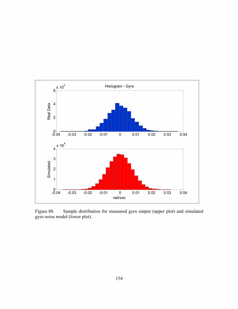
154

-0.04 -0.03 -0.02 -0.01 0 0.01 0.02 0.03 0.040

2

4

6x 10

4

Rea

l Dat

a

Histogram - Gyro

-0.04 -0.03 -0.02 -0.01 0 0.01 0.02 0.03 0.040

1

2

3

4x 10

4

rad/sec

Sim

ulat

ed

Figure 80. Sample distribution for measured gyro output (upper plot) and simulated gyro noise model (lower plot).

155

0 5 10 15 20 25-100

-80

-60

-40

-20Power Spectral Density Estimate - Magnetometer

dB(g

auss

)2 /Hz

PSD of Magnetometer Output297,747 samplesFs = 50 Hz, Total time 1 hr 35 min

=0.1574

=0.0008212

0 5 10 15 20 25-100

-80

-60

-40

-20

dB(g

auss

)2 /Hz

Frequency (Hz)

PSD of Simulated Magnetometer Noise297,747 samples

Figure 81. PSD of measured magnetometer output (upper plot) and simulated magnetometer noise model (lower plot).

156

0.153 0.154 0.155 0.156 0.157 0.158 0.159 0.16 0.161 0.162 0.1630

2

4

6x 10

4

Rea

l Dat

a

Histogram - Magnetometer

0.153 0.154 0.155 0.156 0.157 0.158 0.159 0.16 0.161 0.162 0.1630

1

2

3

4x 10

4

Gauss

Sim

ulat

ed

Figure 82. Sample distribution for measured magnetometer output (upper plot) and simulated magnetometer noise model (lower plot).

E. PNS PERFORMANCE USING THE THREE-DIMENSIONAL FOOT MOTION MODEL WITH NOISE

Now that a complete three-dimensional model for the foot motion acceleration

has been presented, which also includes a random component to simulate the sensor

error, we can begin the examination of the PNS performance. For convenience, the main

features of the motion model are shown in Table 9. In addition to these features, it is also

noted that the walking motion occurs in a straight line in a northerly direction. A useful

feature of our model is that the number of walking steps may be easily varied as desired,

as well as, and for the nine sensors within the IMMU.

157

Table 9. Summary of foot motion acceleration model.

Model Gaussian

Stride length 1.2 m

Vertical displacement 0.25 m

Duration of step 1.0 sec

Duration of swing phase 0.4 sec

Sampling frequency 50 Hz

Accelerometer error = 0.1% of full scale

20.0325m s

Magnetometer error = 0.1% of full scale

30.8212 10 Gauss

Gyro error 67.2 10 rad s

0.0077 rad s

To begin examination of the PNS performance, first we consider the case where

the walking motion occurs in the absence of any sensor error, as shown in Figure 83. The

simulation presented was for a 100-step straight-line walk in the northerly direction.

Total distance error was 3.33 meters for the 120-meter walk. In spite of the noiseless

sensors used in this simulation, an error of 2.8 % still resulted. The source of this error is

due to a number of reasons. It is well known that the selection of numerical integration

method and sampling interval play a significant role in the resulting error; however, as

was learned from the previous discussion in Section B of this chapter, the particular

choice of the acceleration model and the manner in which the samples are distributed also

play a role in the final error. Therefore, while it may not be readily determined which of

158

these factors plays the larger role in the resulting error, it must be acknowledged that

there is some degree of error in the present simulation in which error-free sensors are

considered.

-1 -0.8 -0.6 -0.4 -0.2 0 0.2 0.4 0.6 0.8 10

20

40

60

80

100

120X-Y Position

EAST (meters)

NO

RT

H

(met

ers)

Figure 83. PNS track of a 100-step straight-line walk in the northerly direction with no sensor error in the IMMU.

Next, we consider the case where sensor error is included in the foot motion

model. The following figure examines cases where a proportional amount of sensor error

has been included is shown. For these simulations, only a value for , which was

derived from the measured data for each sensor type, was used, and was set to zero for

these trials. The plots also show each simulation repeated 50 times to gain some sense of

the statistics of the result. A sensor error scale factor was incorporated to examine the

effects of increased or decreased sensor noise in the PNS algorithm.

159

The results of these simulations are shown in Figure 84. Subplot (a) is the case

where no sensor noise was included, and is the same result as that shown in the previous

figure. Subplots (b), (c) and (d) show the results when the sensor error scaling factor was

set to 0.1, 1, and 10, respectively. Consistent with one’s intuition, as the sensor noise is

increased, there is a corresponding increase in the resulting position error, as can be seen

qualitatively in the figure. The spread of the position error in the East/West direction can

be seen to increase as the sensor error scale factor is increased. Table 10 shows the

pertinent statistics of these simulation results.

-1 0 10

20

40

60

80

100

120

NO

RT

H

(met

ers)

(a)

-1 0 10

20

40

60

80

100

120

EAST (meters)

NO

RT

H

(met

ers)

(c)

-1 0 10

20

40

60

80

100

120

EAST (meters)

(d)

-1 0 10

20

40

60

80

100

120

(b)

Figure 84. Simulation results for fifty 100-setep straight-line walks, (a) no sensor error, and sensor error scale factor equal to (b) 0.1, (c) 1, and (d) 10.

160

Table 10. PNS error performance due to varying sensor error scale factor.

East/West Error (meters)

North/South Error (meters) Sensor Error

Scale Factor

No sensor error 0 --- 3.33 ---

0.1 0.00041 0.0035 1.75 0.011

1 -0.0040 0.041 1.76 0.012

10 -0.094 0.35 1.79 0.05

Referring to the table above, for the East/West error, the standard deviation of this

figure increases in proportion to the sensor error scale factor. For the mean value of the

East/West error, on the other hand, we would expect a result near zero, since that is what

was used for the sensor error. More simulations would be required to verify whether this

is true. Interestingly, the mean value of the North/South error does not seem to depend

on the sensor error scale factor, but it is, however, reduced from the case of no sensor

error. While it is not determined with certainty, this behavior may be attributed to what is

referred to as dithering, wherein noise is intentionally added to a system to achieve an

improved performance [91].

Next, we consider the inclusion of or sensor bias in the sensor data. For the

gyros, the measured value is used in the simulations. However, since it was not possible

to measure a corresponding for the accelerometers and magnetometers, a nominal

value will be used in its place that is proportional to the full scale range of each sensor. A

value of 0.1 % of the sensor full scale range is selected. The sensor error scale factor,

which only affects for each sensor type, is set equal to one. Figure 85 and Table 11

show the results of these simulations. Comparing this figure with the results shown in

Figure 84 indicates that the sensor bias introduces a drift or bias into the PNS-computed

track.

161

-2 0 20

20

40

60

80

100

120

NO

RT

H

(met

ers)

(a)

-2 0 20

20

40

60

80

100

120

(b)

-2 0 20

20

40

60

80

100

120

EAST (meters)

NO

RT

H

(met

ers)

(c)

-2 0 20

20

40

60

80

100

120

EAST (meters)

(d)

Figure 85. Simulation results for fifty 100-step straight-line walks with sensor error scale factor equal to one and (a) accelerometer bias only, (b) gyro bias only, (c) magnetometer bias only, and (d) all sensor biases included.

Table 11. PNS error performance with sensor error scale factor equal to one and varying sensor biases.

East/West Error

(meters)

North/South Error

(meters)

Sensor Error Scale Factor

= 1.0 Accel bias

(0.1% full scale) -2.18 0.036 -1.83 0.012

Gyro bias (measured)

-0.0006 0.035 -1.75 0.012

Mag bias (0.1% full scale)

1.17 0.044 -1.76 0.012

All sensor biases included

-0.97 0.036 -1.82 0.011

162

In addition, if one compares Table 11 with the case for sensor error scale factor

equal to one in the pervious table, it is noted that the spread, , for the East/West error

remains relatively unchanged, however, the mean error has been significantly affected by

the inclusion of the sensor bias. It would not be entirely appropriate to try to assess the

sensitivity of this bias error to the biases introduced into the three sensor types because an

accurate measurement for the accelerometer or magnetometer biases could not be

acquired, and we arbitrarily chose to use a figure of 0.1% of sensor full scale instead. It

is illustrative, nonetheless, the manner in which the sensor error bias impacts the overall

error of the PNS.

In the following plots, the effect of the sensor error on the PNS performance is

considered with respect to the number of walking steps. Figure 86 shows the East/West

error for three different cases: 1) no sensor noise, 2) sensor noise included, but =0, and

3) sensor noise and 0. The plot also shows the error (blue diamonds) from three

actual walks, each of approximately 300 steps, around an athletic track. The first two

cases, these are the simulations having zero noise and the other having zero sensor bias,

gave similar error performance. The height of the error bars also is observed to increase

with respect to the number of steps taken, which is indicative of the growth or spread in

the position error with respect to the number of walking steps. This behavior is certainly

consistent with that of inertial navigation systems in general. In the third case, the

simulation included a bias error in the sensors. As noted earlier, the sensor biases

introduce a drift in some particular direction, which is represented in this plot. In fact,

this last simulation result suggests that the PNS performance error may be more sensitive

to these sensor bias errors than to the magnitude of the sensor noise.

163

0 200 400 600 800 1000 1200-2

0

2

4

6

8

10

EW

err

or

(met

ers)

Number of Steps

East-West Error

No noise

Zero biasBias error

Real Walks

Figure 86. PNS East-West error with respect to number of walking steps.

164

0 200 400 600 800 1000 12000

5

10

15

20

25

30

35

NS

err

or

(met

ers)

Number of Steps

North-South Error

No noise

Zero biasBias error

Real Walks

Figure 87. PNS North-South error with respect to number of walking steps.

F. PNS PERFORMANCE WITH REAL DATA

Up to this point, we have examined the performance of the PNS algorithm only

with simulated data. We learned how the sensor noise ( ) affects the performance of the

PNS, and that the spread of the position error will grow with the number of steps taken.

It was also observed that the sensor bias ( ) will introduce a drift into the computed

position in some direction. It may be further inferred that this quantity may have a more

significant impact on the resulting position error than the sensor noise.

Next, in this section we consider the performance of the PNS using actual walking

data from the foot-mounted IMMU. With the new algorithm available for use in our

PNS, the initial position tracks from Chapter II may now be revisited. The IMMU data

from those tracks are applied to the PNS algorithm and compared to the previous results.

First, Figure 88 shows the location where many of the walking trials were conducted. It

165

is a standard athletic track located at Hartnell Community College in Salinas, California.

The circumference of the inner lane is 400 meters. Lane seven, where the walks were

accomplished, is estimated to be 437.50 meters. All walks were conducted in a counter-

clockwise direction. They began and ended at the same point on the track, as shown in

the image.

1. PNS with Constant Gain

Figure 89 was generated using the complementary filter set to a constant gain.

Three different values were used. Immediately upon inspection of the plot, one sees that

the resulting tracks do not resemble the true oval path. When the filter gain was set to

0.15k —recall that this value gave a minimum error in the vertical pendulum—the

algorithm does not produce a satisfactory position track. Two other values of gain were

considered, 0.001k and 0.5k . Neither one of these values produced an acceptable

result. In fact, when 0.001k , the computed track drifted off in a direction away from

the true closed path.

Figure 88. Athletic track used for PNS walking trials (From [92]).

SSttaarrtt//SSttoopp

166

Figure 89. PNS tracks using a constant-gain complementary filter.

2. PNS with Adaptive Gain

Next the PNS is evaluated with an adaptive gain strategy. The filter gain will be

switched between two values according to the gait-phase detection algorithm. When the

foot is in the stance phase, the gain is set to a nominally high value. This is where the

motion-induced accelerations are lower, and the FQA produces better results. During the

swing phase, the foot is moving through the air experiencing rapidly changing

acceleration, and the filter gain is set to a low value such that more of the dynamic

quaternion is represented in the filter output.

Figure 90 shows the computed position for the three walks around the athletic

track. The dashed lines are those that were produced with the proprietary quaternion.

Solid lines represent the tracks computed using our complementary filter with adaptive

gain. Qualitatively, these tracks represent a marked improvement over those computed

-150 -100 -50 0 50 100 150 200-150

-100

-50

0

50

100

150

East (meters)

Nor

th (

met

ers)

k=0.15

k=0.001

k=0.5

167

using the constant-gain filter and those produced with the proprietary quaternion. The

overall shape and orientation of the computed tracks appears very similar to the athletic

track shown in Figure 88.

-100 -50 0 50 100-40

-20

0

20

40

60

80

100

120

140

160

East (meters)

Nor

th (

met

ers)

Walk 1 MS

Walk 2 MS

Walk 3 MS

Walk1 CPF

Walk 2 CPF

Walk 3 CPF

Figure 90. Comparison of position track using adaptive-gain complementary filter (solid) and proprietary algorithm (dashed).

The following tables make a more quantitative comparison of these position

tracks.

Table 12 shows the results for the tracks that were computed using the proprietary

quaternion (dashed lines in Figure 90). The Distance column is the computed distance

traveled for a given walk. Recall that the estimated path length was 437.50 meters.

Using this value, the Distance Error was derived and also included in the table. Another

parameter, XY , is the computed position at the end of each walk. Since all walks began

168

and ended at the same point on the track, this figure represents the radial distance to the

origin. The last column is a position error based on the total distance.

Table 13 has the same information as the previous table, but represents the

performance of the adaptive-gain complementary filter. Comparing the Distance Error

columns from both tables, the adaptive-gain complementary filter has better performance

by almost an order of magnitude. Secondly, the last column of each table, which has the

position error of distance walked, shows that the new filter reduces this error by almost

half.

Table 12. PNS performance using the proprietary algorithm.

Proprietary Algorithm

Distance (m)

Distance Error

ΔXY (m)

% Error of Distance Walked

Walk 1 445.95 1.9% 7.73 1.8%

Walk 2 446.72 2.1% 10.53 2.4%

Walk 3 446.15 1.9% 14.25 3.3%

Table 13. PNS Performance using the adaptive-gain complementary filter.

Adaptive-Gain Complementary Filter

Distance (m)

Distance Error

ΔXY (m)

% Error of Distance Walked

Walk 1 438.43 0.21% 2.52 0.58%

Walk 2 439.30 0.41% 3.37 0.77%

Walk 3 438.35 0.19% 4.84 1.10%

169

G. SELECTION OF THE APPROPRIATE GAIN

The last section showed that the performance of the PNS is greatly improved

when an adaptive gain strategy is utilized. In this approach, two gain values are required,

sk and dk . The former is used when the accelerations are low, as in the foot’s stance

phase, while the latter is used during the foot’s swing phase. To determine the values of

the filter gain that produce the best results, a simple optimization study was

accomplished.

During each iteration of the optimization loop, two filter gain values were

selected, one for sk and one for dk , from a set of possible gains; then the corresponding

position error was computed using the PNS algorithm. Each point spanning the range

0.6 ...1.6sk and 0 ... 0.02dk was considered in the optimization. Since the track

started and ended at the origin, then the final position error was simply

2 2( ) ( )n n nx f y fp p t p t (4.19)

where ( )nx fp t is the last value of the computed position in the nx direction, and ( )n

y fp t is

the last position value in the ny direction. The vertical direction was not considered

because the athletic track was locally flat. Consequently, it was not considered prudent to

include the inaccuracies that may exist in the vertical channel in this study.

Figure 91 shows the result of this optimization study. For each pair of gains,

sk and dk , the computed position error was plotted in the vertical axis of the mesh plot.

The horizontal axes are labeled as sk and dk . The plot shows that a minimum error is

produced when 0dk and 1.05sk . Figure 92 gives a better view of the plot with

respect to sk . It is from here that the value for sk may be estimated more accurately. The

170

lowermost curve in this plot corresponds to 0dk and 0.6 ...1.6sk . Inspection of

this curve supports the idea that a value of approximately 1.05sk gives the minimum

error.

0.51

1.52

00.005

0.010.015

0.024

5

6

7

8

9

10

11

kskd

Err

or

Figure 91. Optimization of the adaptive gain in the complementary filter.

Comparing these values to the result of the pendulum optimization, where we

learned that setting the gain equal to 0.15 gave a minimum pendulum angle error, we see

that for walking motion, setting the filter gain to zero ( 0dk ) during the swing phase

produces better results. During the swing phase, the foot acceleration is changing very

rapidly, and the accelerometers output is comprised of a larger part that arises from this

motion and a smaller part that comes from the gravity vector. As a result, the FQA gives

large errors at this point in the foot motion. In spite of the gyro biases and its associated

error, the errors occurring in the FQA during the swing phase assumedly dominates that

171

which arises from the angular rate sensors. Consequently, setting 0dk during the swing

phase here produces better results than the gain value found in the pendulum motion

experiments.

During the stance phase, when the motion-induced accelerations are lower, it is

beneficial to have a larger component of the filter output derived form the FQA. Setting

1.05sk during this period of the walking motion gives good results. However, as

shown in the plot, a value larger than this is not desirable because the error is seen to

increase. If the foot velocity is zero during this period, then why should the error

increase as more of the FQA quaternion is passed to the filter output? This is possibly

due to the fact that during the stance phase of normal walking, while the foot translational

velocity is zero, its angular velocity is not. In this phase, the foot is rotating from the heel

to the toe in preparation for the next step. If we compare this motion to that of the

pendulum, then the foot will experience some normal and tangential acceleration that will

affect the overall accelerometer output. Thus, the optimization shows that for this phase

of walking motion, it is better to have a blended filter output consisting of both the

dynamic and static quaternions.

172

0.6 0.7 0.8 0.9 1 1.1 1.2 1.3 1.4 1.5 1.64

5

6

7

8

9

10

11

ks

Err

or

kd = 0.02

kd = 0

Figure 92. Selection of sk . Minimum error when 0dk and 1.05sk .

H. ADDITIONAL COMMENTS ON THE PNS PERFORMANCE

In this section, we want to make some final observations on the PNS

performance. Figure 93 shows an expanded view of the Start/Stop region of Figure 90.

The endpoint for each of the three walks is marked with an ‘x’ in the figure. It is

observed that the endpoints all lie in a region west of the origin. Recalling the impact of

the calibration error ( ) introduced into the foot motion model simulations, it is

surmised that the fashion in which these endpoints arise is also due to some calibration

error or sensor bias existing in the actual IMMU.

173

-6 -4 -2 0 2 4-2

-1

0

1

2

3

4

5

6

7

8

East (meters)

Nor

th (

met

ers)

Start/Stop

Walk 1

Walk 2

Walk 3

Figure 93. Zoom of Figure 90. PNS-computed endpoints marked with an ‘x’.

In Figure 94, a comparison is made with a track acquired from GPS (shown in

black). No quantitative performance has been provided, but this plot is included here to

give an overall impression of the PNS performance. In addition to the PNS error, there

are two potential sources of error in this plot that must be acknowledged. The first source

of error comes from the fact that the PNS track is computed with respect to magnetic

north, while the GPS track is with respect to true north. In order for a comparison to be

made between the two tracks, the PNS track was rotated by an amount equal to the local

angle of declination, the precision of which can not be easily quantified. A second source

of error comes from the need to convert the latitude/longitude coordinates derived from

GPS into linear distance units of meters. This further requires an estimate of the earth’s

radius, which is on the order of 6367 km and is a potential source of error if not

quantified accurately. In spite of these concerns, the figure illustrates qualitatively that

the results from the PNS algorithm are roughly in agreement with the GPS track.

174

-50 0 50 100-40

-20

0

20

40

60

80

100

120

140

160

East (meters)

Nor

th (

met

ers)

CF

GPS

Figure 94. Comparison of PNS track (red) with GPS track (black).

Figure 95 shows the Microstrain 3DM-GX1, which has been the primary sensor

used throughout the scope of this project. Also shown in the figure is a smaller version of

an IMMU from MEMSense. The MEMSense nIMU has three sets of orthogonally-

mounted accelerometers, magnetometers, and angular rate sensors. It is approximately

90% smaller by volume than the 3DM-GX1. Data is available to the user through an

inter-integrated circuit (I2C) interface at 150 samples per second. Although it does not

compute quaternions for the user, as does the 3DM-GX1, its smaller size makes it

attractive for this application.

175

Figure 95. MEMSense nIMU (lower) and Microstrain 3DM-GX1 (upper).

This IMMU was used in several walks around the same athletic track, the results

of which are shown in Figure 96. Two observations are made here. First, the resulting

plots appear to reproduce the actual walking path around the athletic track, thus

reinforcing the utility of the PNS algorithm. A second observation deals with the

sampling frequency. In spite of the higher sampling rate provided by this IMMU, the

results are not necessarily significantly improved—a point borne out in the simulation

study presented earlier in this chapter.

176

-120 -100 -80 -60 -40 -20 0 20 40 60 80

-20

0

20

40

60

80

100

120

140

East (meters)

Nor

th (

met

ers)

Hartnell College Athletic Track, MEMSense IMMU

walk1

walk2

walk3

MEMSense IMMUwith adaptive gaincomplementaryfilter

Figure 96. PNS-computed track using MEMSense IMMU.

One final thought on the PNS performance is given. It deals with the manner in

which the endpoints of the computed tracks all fall in the same region with respect to the

origin. Figure 97 shows an expanded view of the previous figure. As before, the

endpoints are marked with an ‘x’; similar to the results when the 3DM-GX1 was used, all

three endpoints are clustered in the same area relative to the start/stop point. Recalling

the previous simulations using the foot motion acceleration model, this behavior is quite

likely due to a degree of uncorrected sensor bias or calibration error within the IMMU.

In spite of our best efforts to eliminate these errors with the zero-velocity updates,

evidently, some portion still remains. Furthermore, the figure suggests that a larger

component of the PNS error is derived from the sensor bias than from the random noise.

177

-20 -10 0 10 20-15

-10

-5

0

5

10

15

20

25

30

35

East (meters)

Nor

th (

met

ers)

Start/Stop

Hartnell College Athletic Track, MEMSense IMMU

walk1

walk2

walk3

MEMSense IMMUwith adaptive gaincomplementaryfilter

Figure 97. Zoom of Figure 96. PNS-computed endpoints marked with an ‘x’.

I. SUMMARY

This chapter presented the PNS algorithm and explored its performance through

simulations and with the aid of actual walking data. A foot motion model was developed

specifically for use in these simulations. It was built upon the Gaussian exponential

function. The simulation also included a carefully selected model for the sensor random

error. The parameters of the random error were varied to study their impact on the

overall performance of the PNS. This chapter also examined various techniques for

numerical integration to use in the strapdown portion of the PNS algorithm. The

Trapezoidal rule was found to be adequate for this application and the sampling rate of 50

samples-per-second was considered sufficient for normal walking motion.

A qualitative comparison of the PNS with a constant-gain complementary filter

and the adaptive-gain complementary filter was also provided. It showed that the latter

178

approach gave superior performance and created position tracks that were more

representative of the true tracks. In the adaptive-gain complementary filter, the gain was

adaptively switched between two values in accordance with the particular phase of the

gait cycle. An optimization was accomplished using the actual data; it indicated that

using 0dk and 1.05sk gave the minimum position track error.

This chapter concluded by examining the endpoints of the walking trials around

the athletic track. The manner in which the endpoints all tended to be grouped together

in the same area suggested that there was a component of the sensor error that could not

be negated by the zero-velocity updates.

179

V. A LOCOMOTION INTERFACE FOR THE VIRTUAL ENVIRONMENT

The major theme of this dissertation has been the development of the PNS. The

complementary filter and its integration with the strapdown navigation algorithm has

been the focus of the discussion to this point. It was during the course of this work that

another application for the IMMU came to light. Methods for interaction with virtual

environments are essential to enhance the utility of these computer-generated realities.

This chapter presents a novel locomotion interface based on the IMMU that allows one to

navigate through the virtual environment.

A. BACKGROUND

A virtual reality is a computer-generated environment. Its purpose is to provide

either entertainment or some form of training and education. Another application that has

gained interest in the medical community is for the treatment of post-traumatic stress

disorder in soldiers.

In order for the user of a virtual environment of have a positive and rewarding

experience, he/she must have a high sense of presence. This is the subjective measure of

one’s feeling that he/she really is in the virtual reality. Presence depends on the amount

of immersion offered be the virtual environment. Therefore, immersion is the objective

measure of the amount of sensory stimuli provided by the virtual environment.

To achieve the desired high levels of presence, researchers have worked to

develop immersion devices of various types. These devices are designed to stimulate the

senses and promote a more realistic experience within the virtual environment. The most

common types of user interfaces are those that are found on almost any desktop having a

computer. They are the computer monitor, keyboard, mouse, and speakers. However,

these do little to heighten user presence. More advanced types of interfaces have been

developed. To display graphics to the user, one of two methods has been used. A head

mounted display can be used, which tracks the user’s head motion and renders the display

consistent with the head orientation (see Figure 3). Alternatively, the virtual environment

180

can be displayed in a large screen immediately in front of the user, or in other cases, a

multi-projector (display) screen can also be utilized. In this approach, the user is

presented with a scene that fills his/her peripheral vision as much as possible with two or

more large projector screens/displays.

To stimulate the sense of smell while engaged within a virtual environment, the

Army developed a device called the “scent collar.” This device was worn around the

user’s neck and dispensed an odor that was relevant to the location within the virtual

environment [92]. At appropriate times, the “scent collar” released a scent pertinent to

the particular environment to further enhance the user’s sense of presence.

In addition to the use of graphics, sound, and smell to increase the sense of user

presence in a virtual environment, the control of motion is also just as important. Popular

forms of user interfaces for motion control include joysticks and game controllers.

However, as studied in [93] and [94], user presence is increased when his/her motions

through a virtual environment are similar or identical to those required for the same

movement through a real environment. For example, when the user is required to walk or

walk-in-place to simulate virtual walking, this results in a greater sense of presence than

if the user were required to simply move a joystick or strike one of the arrows on the

keyboard to move forward. To this end, other types of motion control devices, or

locomotion interfaces, for virtual environments have been developed. Many are

variations of treadmill designs, assumedly because this required body motions most like

those exhibited in the real world and would most likely result in a high sense of user

presence. Other designs are based on step-in-place devices, where the user steps on pads

located on the floor to direct his/her motion through the environment.

1. Treadmills

Several examples of locomotion interfaces have been constructed that utilize

treadmills. One of the first of this type was developed for the Army by Virtual Space

Devices, Inc., see Figure 98 and [95]. This device was called the Omni-Directional

Treadmill, or ODT. It allowed the user to move in any direction on the treadmill surface,

and through a feedback control mechanism, it maintained the user in a relatively

stationary location. A tracking arm attached to the user measured the user’s position and

181

orientation. These data were then passed into the control algorithm to move the treadmill

in the appropriate direction, thus keeping the user fixed in the center of the treadmill

surface. A novel aspect of this approach was that it incorporated two orthogonal

treadmills—one treadmill made up of a number of smaller treadmill belts that were

installed orthogonal to the main one. A variation to this approach comes from Iwata [96]

in what was called the Torus Treadmill. This version of the locomotion interface used

Polhemus position trackers on the user’s knees, so the attachment of a tracking arm to the

user was not required. This was to give the user greater freedom of movement.

Figure 98. Omni-directional treadmill (From [98]).

Another very interesting treadmill approach was developed by [97]. Referred to

as the Ground Surface Simulator (GSS), this design incorporated the results of two

previous projects, the ATLAS [98] and ALF [99]. ATLAS was a treadmill design that

was mounted onto a 3-DOF rotating platform. Infra-red reflectors attached to the user’s

feet were tracked via an infra-red CCD camera. The corresponding foot tracking data

were then used to move the treadmill forward and to rotate the entire treadmill in a

horizontal plane to simulate changes in the walking direction. The ALF was a floor

182

design that consisted of an array of movable tiles. When activated, the individual tiles

could be raised or lowered to simulate a varying roughness of terrain.

Yet another use of the treadmill for the locomotion interface was created by

[100]. This design, called the Sarcos Treadport, was unique in that it used a mechanical

tether that was attached to the user to measure position and orientation on the treadmill.

This information was used to control the speed of the treadmill as the user walked and to

rotate the projected virtual environment when the torso was rotated in a particular

direction. The mechanical tether also applied force feedback to the user’s torso. In this

manner the inertial forces one senses during acceleration and deceleration could be

transmitted to the user to enhance the overall sense of presence.

2. Step-In-Place and Gesture Recognition

The use of the treadmill as part of a locomotion interface has been popular

because this device allowed the user to move through the virtual environment in a very

natural way. However, as was acknowledged in many of the references, in its

implementation, a considerable amount of engineering design was required to control the

treadmill speed and further, to determine the direction of motion. Other designs have

been proposed that do not use the treadmill or a treadmill derivative. These consist of

either some type of pad or platform on which the user was required to stand or march in

place. The Walking-Pad, as described in [101], measured 45-cm x 45-cm and consisted

of an array of 64 switches. As the user marched in place on the pad, the corresponding

switches that were activated beneath each foot were used to compute a location for the

center-of-gravity on the pad. The position of the center-of-gravity was then used to

determine a direction of motion through the virtual environment.

The Virtual Perambulator [102] was a design that required the user to wear a pair

of sandals on which a low-friction film had been installed on the sole. The user slid

his/her feet across a special floor pad. Polhemus FASTRACK sensors on each foot were

used to determine the length and direction of steps as the user slid their feet across the

surface. A waist-high stabilizing bar that surrounded the user was utilized for the user to

hold while they moved and to provide a measure of safety.

183

In the Step-in-place Turntable [103], the user stood on a 70-cm diameter

motorized platform. Pressure sensors in the platform sensed when the user was stepping

and propelled the user forward in the virtual environment. To determine direction,

infrared markers at the back of the person’s waist were monitored by an infrared camera.

As the user rotated his/her torso, as if to turn, the relative position of the markers in the

camera’s field of view registered this rotation. This information then caused the

motorized platform to rotate in the opposite direction to bring the user back into view of

the large projected screen.

A novel locomotion interface, called CirculaFloor, was developed by [104]. It

utilized a set of automatically positioning floor tiles. As the user began to move from the

center of the floor tile upon which he stood, the underlying control system would

automatically move one of the unused floor tiles into a position to receive the user as they

left the first floor tile. The system used ultra-sonic sensors on the floor tiles to monitor

their position in the active floor space. The user’s position was monitored within the

active area with a laser radar system. See Figure 99.

Figure 99. CirculaFloor designed by Iwata (From [104]).

In [105], a pair of CyberBoots was constructed. Four force sensors were

distributed in the insole of each boot. A fuzzy logic algorithm was then implemented to

classify the user motion as either leaning or walking for interaction with a virtual object.

184

In another locomotion interface known as Gaiter, see [48], the system used pressure-

sensitive foot switches, along with position and orientation tracking sensors attached at

the knees, waist, and head, to move the user through the virtual environment, which was

presented in the head mounted display.

B. SYSTEM DESCRIPTION

At the Naval Postgraduate School, we have developed a locomotion interface for

an existing marksmanship training system. In this training system, the user was required

to stand in front of a large projector screen (approximately 8 ft x 8 ft) onto which was

projected a virtual environment of a fictional urban setting. The user was equipped with

a simulated M-16 rifle that shot rounds of laser pulses. Targets that were projected onto

the screen were then shot at with the M-16 rifle. A camera monitoring the screen

captured the location of the incident laser pulses on the screen for correlation with the

actual target location. The locomotion interface, known as MOVESMover, used two

IMMU devices—one on each foot. Through a series of foot gestures, the user was free to

navigate in a desired direction through the virtual environment. This approach was

appropriate for our marksmanship training system because it allowed the user to maintain

his position and orientation immediately in front of the projector screen. Furthermore, he

could change his direction of walking through the virtual environment without having to

rotate any part of his head or torso and possibly take his eyes away from the simulated

targets.

In the MOVESMover locomotion interface, the user stood in front of a large

projection screen onto which a virtual environment had been displayed. As the user

gestured with his/her feet, the projected scene within the virtual environment changed

accordingly and provided the user with the perception of movement through the virtual

environment. The foot gestures required of the user are shown in Table 14, along with

the corresponding movement that resulted in the virtual environment.

185

Table 14. MOVESMover foot gestures.

User Foot Gestures Motion in VE

No foot motion Not walking

Marching in place Walking forward

Left foot step, right foot yaw Walking turn- forward right

Right foot step, left foot yaw Walking turn- forward left

Right foot step only Side step right

Left foot step only Side step left

Right foot yaw only Turn in place, clockwise

Left foot yaw only Turn in place, counter-clockwise

Figure 100 shows the system hardware. The user wore one IMMU on each foot,

such as the Microstrain 3DM-GX1. A Sony UX180P mobile computer, which was

carried by the user in a pouch or backpack, read the sensor data from each foot through a

RS232-to-USB interface. The mobile computer executed the custom C++ program

referred to as the MOVESMover application in which it accomplished the following

tasks: 1) read the sensor data from both feet, 2) decoded the foot gestures into one of the

eight motions for the Delta3D virtual environment, and 3) transmitted the commanded

movement via wireless network to the Delta3D PC. The Delta3D PC rendered the virtual

environment according to the movement information that it received from the mobile

computer.

186

Figure 100. System hardware used in MOVESMover.

In order to decode the foot gestures into one of the eight motions for movement

through the virtual environment, a series of state machines were implemented in the

MOVESMover application. These state machines, as shown in Figure 101, worked

together to produce one of the eight possible movements. As an illustration of how these

state machines worked together, the Swing/Stance state machine for the left foot

identified periods of foot swing and foot stance. Then the Motion/~Motion state machine

for the same foot determined whether the foot was in a general state of motion over one

or more cycles of the Swing/Stance state machine. An identical pair of state machines

was created for the right foot. In this manner, it was possible to determine sustained

periods of foot motion for each foot.

If the user gestured in a repeated twisting motion (by an outward rotation of the

ankle so that the foot rotated in a plane parallel to the ground), the Yaw/~Yaw state

machine was triggered. One state machine of this type was created for each foot. These

state machines, along with the Motion/~Motion state machines for both feet, worked

together in what was referred to as the Overall state machine to classify the foot gestures

into one of eight movements through the virtual environment.

IEEE 802.11

Sony UX180P Wireless router

PC with Delta3D application

Virtual environment rendered by the Delta3D PC and projected onto a large screen

User wears one sensor on each foot. MOVESMover application runs on mobile PC.

ethernet

187

Figure 101. State machines for the MOVESMover locomotion interface.

SWING STANCE

Left Foot Swing/Stance State Machine

MOTION ~MOTION

Left Foot Motion/~Motion State Machine

Swing/Stance S.M. drives the Motion/~Motion S.M for the left foot

SWING STANCE

MOTION ~MOTION

Swing/Stance S.M. drives the Motion/~Motion S.M for the right foot

Right Foot Swing/Stance State Machine

Right Foot Motion/~Motion State Machine

YAW ~YAW

Left Foot Yaw State Machine

~Walking

Walking Straight

Walking Fwd Right

Walking Fwd Left

Side Step Left

Side Step Right

Turn in Place CCW

Turn in Place CW

YAW ~YAW

Right Foot Yaw State Machine

Overall State Machine (yellow) is driven by the subordinate S.M.’s, as indicated by the dashed arrows

188

In Figure 102, a portion of the state machine operation in shown. It shows the

angular rate data for three steps of the left foot (Figure 102a). Through experiment, it

was learned that using the foot angular rate instead of acceleration produced more

consistent identification of the periods of foot swing and foot stance. Figure 102b shows

the cycles of the Swing/Stance state machine over the three steps. This state machine

compared the angular rate with a specified threshold, which was also determined

experimentally. If the angular rate exceeded the threshold for a defined period of time,

the state machine switched into the Swing state. Alternatively, if the angular rate fell

below the established threshold for a period of time, the state machine switched to the

Stance state. Subsequently, the Motion/~Motion state machine used the status of the

Swing/Stance state machine to make its determination of sustained foot motion, as

observed in Figure 102c. It accomplished this by considering whether the Swing/Stance

state machine was persistent in the Stance state over an interval of time. Furthermore, if

the Swing/Stance state machine switched to the Swing state, the Motion/~Motion state

machine immediately changed into the Motion state.

The operation of the yaw state machine is shown in Figure 103. It shows the foot

yaw angle data. This parameter was derived from the sensor’s computed orientation (i.e.

quaternion). In Figure 103a, the user was executing a series of quick ankle twists. As

shown, there existed an approximate offset of (-)2.5 radians in this sample of data. It was

in essence the horizontal direction in which the foot sensor was oriented with respect to a

North-East-Down coordinate system when the foot was in the Stance state. On occasion,

this offset was also observed to exhibit a slow wander. It was surmised that this behavior

resulted from the sensor’s orientation algorithm and its difficulty to track the erratic foot

motions. To alleviate this problem, a first-order high-pass filter was used on the foot yaw

data. This filter was implemented as shown below with 0.9 .

1 1k k k ky y x x (5.1)

189

0

2

4

6

Step 1

Step 2 Step 3

(a)ra

d/se

c

0

1

stance

swing

stance

swing

stance

swing

stance

(b)

Sw

ing/

Sta

nce

0

1

~motion

motion

~motion

(c)

Mot

ion/

~M

otio

n

Figure 102. Three steps of the left foot and classification by the corresponding state machines.

-5

0

5

(a)

rad

-1

0

1

(b)

rad

0

1

(c)

Yaw

/~Y

aw

Figure 103. Filtering of the foot yaw data and classification by the Yaw/~Yaw state machine.

190

The resulting filter attenuated all frequencies below approximately 0.5 Hz (Fs =

30 Hz), and Figure 103b shows the filtered foot yaw with the offset removed. This data

was then used in the Yaw/-Yaw state machine. It was compared with a threshold and the

Yaw state was set accordingly, as shown in Figure 103c.

During each program cycle, the Overall state machine used the current status of

the four collaborating state machines to make its determination of the movement through

the virtual environment. The result was then transmitted via a network UDP packet to the

Delta3D PC, which in turn rendered the virtual environment for the user. The transmitted

data consisted of two short data types. The first parameter was an integer value between

0 and 7 that corresponded to one of the motions shown in Table 14. The other parameter

corresponded to a speed to which the user moved through the virtual environment. This

latter parameter was a fixed value, thus it was not computed from the rate of movement

of the user’s foot gestures. Experiment and data analysis to compute a user’s speed

through measurement of the rate of one’s foot gestures failed to yield any good results.

The sample rate of approximately 30 Hz from each sample proved insufficient to achieve

accurate measurements of rates of one’s foot gestures.

C. SUMMARY

We have developed a low-cost locomotion interface for a virtual reality

marksmanship trainer. The MOVESMover locomotion interface required the user to

utilize foot gestures for motion control through the virtual environment. Admittedly, the

ideal locomotion interface would have been one that required the user to walk as in the

real world. However, since this was not possible for our application, a good engineering

compromise was achieved with our approach. In addition to low-cost, the

MOVESMover locomotion interface was easily implemented in that it used commercial

off-the-shelf equipment and only required the development of a custom computer

program to decode the sensor data appropriately. Because the foot-worn sensors were

inertial/magnetic, there was no requirement for the installation of any infrastructure, other

than the wireless network to transmit the data. The MOVESMover locomotion interface

was demonstrated at the MOVES Institute Open House in July 2008. Preliminary trials

191

of the interface indicated that after approximately two or three minutes, users who tried

the locomotion interface became accustomed to the required foot gestures and moved

confidently through the virtual environment.

192


193

VI. CONCLUSION AND RECOMMENDATIONS

This chapter provides final conclusions and summarizes the major contributions

of this dissertation. Recommendations for future work are also given here. The main

theme of this body of work concerned the Personal Navigation System (PNS), which

gave the user a capability of tracking one’s position in GPS-denied environments.

Another component of this effort was the development of a locomotion interface for a

virtual environment. Both of these elements described within this dissertation utilized the

miniature inertial/magnetic measurement unit (IMMU).

A. SUMMARY OF CONTRIBUTIONS

The primary accomplishment of this dissertation was the design and development

of the Personal Navigation System (PNS) to track one’s position during normal walking.

In this implementation, a miniature inertial/magnetic measurement unit (IMMU) was

utilized. These devices were based on MEMS technology and were small, lightweight,

low-cost, and low-power. However, they suffered from an added amount of sensor error

that was greater than that found in navigation-grade inertial measurement units designed

for military and commercial applications. Consequently, straightforward use of the

miniature IMMU with the well-known strapdown navigation algorithm in a personal

navigation application would lead to rapidly increasing position error. For this reason, a

new navigation algorithm was designed and tested to mitigate the degraded performance

of the miniature IMMU.

The new PNS algorithm was adapted from the strapdown navigation algorithm

and integrated three additional component algorithms. One of these components was an

error-correction technique known as zero-velocity updates, which was used to negate the

accumulation of error in the computed velocity that had resulted from the integration of

the error in the foot-mounted sensor. Another critical component was the quaternion-

based complementary filter. Designed specifically for the PNS, it employed an adaptive

gain-switching strategy and provided the dynamic foot attitude estimate required for the

strapdown navigation algorithm. Lastly, the gait-phase detection algorithm was also

194

incorporated. It identified the instances of the foot stance and swing, which were

required for operation of the complementary filter and the zero-velocity updates.

A significant contribution in support of the PNS development was a measured

improvement in the dynamic performance of the Factored Quaternion Algorithm (FQA)

through its integration in the quaternion-based complementary filter resulting in an

algorithm that facilitated the completion of the PNS. The composite algorithm gave an

intuitive and straightforward method for attitude estimation suitable for applications

beyond those of the PNS application. Testing of the attitude filter was accomplished by

simulation and through the use of an instrumented pendulum built in the laboratory.

The quaternion-based complementary filter incorporated a novel gain-switching

scheme that leveraged the natural features of normal biped walking. This approach was

shown to give improved performance in the PNS over a filter utilizing a constant gain.

Additionally, in support of this contribution a gain optimization was performed using

experimental data to identify the best values for the filter static gain, sk , and the dynamic

gain, dk , that resulted in the minimum position error.

The gait-phase detection algorithm identified instances of foot stance and swing

with a demonstrated high degree of accuracy. Furthermore, it signaled the appropriate

times to employ the zero-velocity updates and also indicated when the gain should be

switched within the complementary filter.

This work also described the development of a foot motion model. Based on the

Gaussian exponential function, it provided a means for simulation of the PNS and gave

insight into the performance of the navigation algorithm. The model also included a

component of sensor error, which was validated through experimental measurement and

analysis.

An investigation of the numerical methods suitable for the PNS algorithm was

also accomplished. Through simulation and experiment, the Trapezoidal rule was shown

to give satisfactory results for the strapdown portion of the PNS application, and Euler’s

method was appropriate for the complementary filter. Furthermore, this work also

highlighted the fact that data sampling rates on the order of 50 samples-per-second were

adequate for a PNS utilized in normal walking conditions.

195

As an incidental by-product of this effort, a novel utilization for the IMMU was

also developed—a locomotion interface for a virtual environment. As in the PNS

application, it used the shoe-worn IMMU. In this application, however, two IMMUs

were required, one to be worn on each foot. A set of foot gestures were conceived and a

custom software program was developed to decode the user’s foot motions. This unique

interface, referred to here as MOVESMover, gave the user freedom to navigate through

virtual environments utilizing large projection displays in which the user was required to

remain in front of the screen. Specifically, the locomotion interface was designed for a

military marksmanship training system that projected virtual targets onto a large

projection display located immediately in front of the trainee.

B. RECOMMENDATIONS FOR FUTURE WORK

It is noted that the PNS was not without its limitations. Firstly, the PNS was only

demonstrated for normal biped walking. Locomotion by other means (i.e. limping,

skipping, hopping) was not considered in this dissertation, but are topics for further study

and development. Performance of the PNS was initially examined for the case of running

motion. It was found that the data sample rate was insufficient to identify the necessary

features of this type of locomotion and was not considered beyond this point. IMMUs

providing higher sampling rates may be worthwhile avenues for investigation, as well as,

tailoring the gait-phase detection algorithm with additional features to recognize the onset

of running and other forms of biped locomotion.

Another operational limitation of the PNS deals with the walking surface. Only

flat, level walking surfaces were examined, such as, concrete or other types of

manufactured flooring (tile, rubberized asphalt). Walking on softer surfaces, grass for

example, made it difficult for the gait-phase detection algorithm to determine the

principal features of natural walking motion and prevented the other components of the

PNS from operating properly. Further investigation and study is required here to build up

this capability within the gait-phase detection algorithm.

PNS performance in terms of heading accuracy is mainly determined by the

magnetometer. This sensor, however, is known to be susceptible to magnetic

disturbances arising from hard-iron or soft-iron interference. A thorough examination of

196

this performance limitation was not accomplished, but is recommended for future work.

It is suggested that further testing be accomplished in a space where the local magnetic

field can be controlled or quantified so that this type of interference on the PNS

performance can be assessed in greater detail. Furthermore, possible solutions to address

this limitation could come in the form of an additional sensor, such as, a high-end angular

rate sensor (fiber-optic gyro) to measure heading rates-of-change. Yet another approach

could involve an examination of the sudden change in the magnetic field due to some

interference and correlate this to angular rate measurements. It is surmised here that a

true heading change would be sensed by the magnetometers, as well as, some component

of the angular rate sensors. On the other hand, if the magnetometers exhibit some change

in their output due to some anomalous interference, the angular rate sensors being

insensitive to the interference would not give any representation of this and could serve

as an indication of the degraded magnetometer performance. Additional features could

be integrated into the PNS algorithm rooted in these ideas and lead to a more robust

navigation system in regions prone to magnetic interference.

While not a limitation of the PNS algorithm, another source of potential

improvement in the overall system deals with the accuracy of the IMMU. Recalling the

figures showing the computed paths around the athletic tracks, they exhibited the

behavior that the endpoints tended to cluster in the same region with regard to the origin.

Furthermore, it was indicated that this pattern was due to the sensor bias, and in spite of

our best efforts to eliminate these errors with the zero-velocity updates, there was still

some part of the bias error that could not be removed. It is put forward that this

remaining error may be addressed through a rigorous calibration of the IMMU sensors.

A study of accepted calibration procedures is necessary and an understanding of the

complex relationship between sensor calibration accuracy and other factors including

temperature and materials aging, among others is warranted.

Many navigation systems incorporate the Kalman filter to improve the overall

accuracy of the computed position. All of these solutions require the use of an additional

navigational aid, such as GPS, to provide measurements of some or all of the components

of the Kalman filter state vector. Since a main motivation of this work was for

197

navigation in GPS-denied environments, the integration of the Kalman filter was not

pursued here. Alternatively, it has been suggested that the zero-velocity updates could be

used in some form to serve as the required navigational aid for the Kalman filter

algorithm. While this idea was not pursued in any detail in this work, it is nonetheless a

very interesting and worthwhile area for further investigation.

The preceding discussion and recommendations were not meant to be

comprehensive. Admittedly, there remains a great deal of additional capabilities required

before a PNS suitable for military application would be available.

198


199

LIST OF REFERENCES

[1] “Navigation,” Encyclopedia Britannica, 15th ed. vol. 24, pp. 756–766. [2] N. Grice, “Sailing the polynesian sky,” Odyssey, April 2004, vol. 13, iss. 4, p. 43. [3] E. Amcoff, “Mobile phones are packing more GPS features,” The Wall Street

Journal, March 23, 2006, p. D2. [4] M. Lehtinen, A. Happonen, and J. Ikonen, “Accuracy and time to fix using

consumer-grade GPS receivers,” Software, Telecommunications and Computer Networks, 2008. SoftCOM 2008, 16th International Conference, September 25–27, 2008, pp. 334–340.

[5] M. S. Braasch and A. J. van Dierendonck, “GPS receiver architectures and

measurements,” Proceedings of the IEEE, vol. 87, iss. 1, January 1999, pp. 48–64.

[6] A. B. Chatfield, Fundamentals of High Accuracy Inertial Navigation, Volume

174 Progress in Astronautics and Aeronautics, American Institute of Aeronautics and Astronautics, Inc., 1997, pp. xiii.

[7] R. G. Brown, Introduction to Random Signal Analysis and Kalman Filtering.

New York: John Wiley & Sons, 1983. [8] M. Kayton, “Navigation Systems,” in The Electrical Engineering Handbook, R.

C. Dorf, Ed. CRC Press, 1993. [9] G. R. Pitman Jr., Inertial Guidance. New York: John Wiley & Sons, 1962. [10] D. Titterton and J. Weston, Strapdown Inertial Navigation Technology, 2nd ed.,

The Institution of Electrical Engineers, Michael Faraday House, United Kingdom, and The American Institute of Aeronautics and Astronautics, USA, 2004.

[11] N. Maluf, An Introduction to Microelectromechanical Systems Engineering.

Massachusetts: Artech House, 2000. [12] H. Weinberg, H., “MEMS sensors are driving the automotive industry,” Sensors

Magazine, February 1, 2002. [13] D. Breed et al., “Method and System for Controlling a Vehicle,” U.S. Patent No.

7,085,637, August 1, 2006.

200

[14] R. A. Wood, “High-performance infrared thermal imaging with monolithic silicon

focal planes operating at room temperature,” Electron Devices Meeting, 1993. Technical Digest., International, December 5–8, 1993, pp. 175–177.

[15] R. P. Lyle and D. Walters, “Commercialization of silicon-based gas sensors,”

Solid State Sensors and Actuators, 1997. Transducers ’97 Chicago, 1997 International Conference, vol. 2, June 16–19, 1997, pp. 975–978.

[16] Knowles Acoustics, “SiSonic surface mount microphones,” July 2003, [Online].

Available: http://www.knowlesacoustics.com/images/pdf/white/Surfacemount.pdf [Accessed: December 1, 2006].

[17] L. J. Hornbeck, “Frame Addressed Spatial Light Modulator,” U.S. Patent No.

4,615,595, October 7, 1986. [18] Texas Instruments, “Digital light processing technology,” [Online]. Available:

http://www.dlp.com/ [Accessed: May 3, 2010]. [19] E. Bassous, “Nozzles Formed in Monocrystalline Silicon,” U.S. Patent 3,921,916,

November 25, 1975. [20] E. Bassous et al., “Jet Nozzle Structure for Electrohydrodynamic Droplet

Formation and Ink Jet Printing System Therewith,” U.S. Patent No. 3,949,410, April 6, 1976.

[21] C. Chiou et al., “Ink Jet Nozzle Structure,” U.S. Patent No. 3,958,255, May 18,

1976. [22] W. A. Wan and M. Lim, M., “Fiber optic Switch Using MEMS,” U.S. Patent No.

6,477,290, November 5, 2002. [23] Yammamoto et al., “Optical Switch Using Tilt Mirrors,” U.S. Patent No.

6,044,705, August 6, 2002. [24] Dautartas et al., “Self-aligning 1xN Rotary Optical Switch,” U.S. Patent No.

6,320,997, November 20, 2001. [25] Rosa et al., “Method for an Optical Switch on a Silicon on Insulator Substrate,”

U.S. Patent No. 6,632,374, October 14, 2003. [26] S. Lucyszyn, “Review of radio frequency microelectromechanical systems

technology,” Science, Measurement and Technology, IEE Proceedings, vol. 151, iss. 2, 2004, pp. 93–103.

201

[27] S. D. Senturia, Microsystem Design. Kluwer Academic Publishers, 2000. [28] D. Tuite, “Motion-Sensing MEMS gyros and accelerometers are everywhere,”

Electronic Design, vol. 57, no. 14, July 9, 2009. [29] J. L. Marins, X. Yun, E. R. Bachmann, R. B. McGhee, and M. J. Zyda, “An

extended Kalman filter for quaternion-based orientation estimation using MARG sensors,” Intelligent Robots and Systems, 2001. Proceedings, 2001 IEEE/RSJ International Conference, October 29–November 3, 2001, vol. 4, pp. 2003–2011.

[30] Analog Devices, Inc., “ADXL325: small, low-power, 3-axis +/-5g

accelerometer,” [Online]. Available: http://www.analog.com/en/sensors/inertial-sensors/adxl325/products/product.html [Accessed: May 3, 2010].

[31] Analog Devices, Inc., “ADXRS610: +/-300 deg/sec angular rate sensor,”

[Online]. Available: http://www.analog.com/en/sensors/inertial-sensors/adxrs610/products/product.html [Accessed: May 3, 2010].

[32] Northrop-Grumman, “LN-200 inertial measurement unit,” [Online]. Available:

http://www.es.northropgrumman.com/solutions/ln200/ [Accessed: May 3, 2010]. [33] W. Stockwell, “Angle random walk,” [Online]. Available:

http://www.xbow.com/Support/Support_pdf_files/AngleRandomWalkAppNote.pdf [Accessed: May 3, 2010].

[34] E. Ogg, “GPS finding its way to the mainstream,” November 15, 2006. [Online].

Available: http://news.cnet.com/GPS-finding-its-way-to-the-mainstream/2100-1041_3-6135918.html [Accessed: May 3, 2010].

[35] Q. Ladetto and B. Merminod, “In step with INS,” GPS World, October 2002, pp. 30–38. [36] “VisuAide unveils Trekker 2.0,” Satellite Today. Potomac, March 18, 2004, vol.

3, iss. 52, p. 4. [37] “Medical Devices: SWAN system provides wearable audio navigation technology

for visually impaired,” Medical Devices and Surgical Technology Week, Atlanta, September 10, 2006, p. 304.

[38] Honda, “ASIMO, the Honda humanoid robot,” [Online]. Available:

http://world.honda.com/ASIMO/ [Accessed: May 3, 2010].

202

[39] E. R. Bachmann, “Inertial and magnetic tracking of limb segment orientation for

inserting humans into synthetic environments,” PhD dissertation, Naval Postgraduate School, Monterey, California, December 2000.

[40] X. Yun, C. Aparacio, E. R. Bachmann, and R. B. McGhee, “Implementation and

experimental results of a quaternion-based Kalman filter for human body motion tracking,” Robotics and Automation, 2005. ICRA 2005. Proceedings of the 2005 IEEE International Conference, April 18–22, 2005, pp. 317–322.

[41] X. Yun, E. R. Bachmann, A. Kavousanos-Kavousanakis, F. Yildiz, and R. B.

McGhee, “Design and implementation of the MARG human body motion tracking system,” Intelligent Robots and Systems, 2004. (IROS 2004). Proceedings. 2004 IEEE/RSJ international Conference, vol. 1, September 28–October 2, 2004, pp. 625–630.

[42] E. R. Bachmann, X. Yun, D. McKinney, R. B. McGhee, and M. J. Zyda, “Design

and implementation of MARG sensors for 3-DOF orientation measurement of rigid bodies,” Robotics and Automation, 2003. Proceedings. ICRA ’03. IEEE International Conference, vol. 1, September 14–19, 2003, pp. 1171–1178.

[43] I. Pantazis, “Tracking human walking using MARG sensors,” M.S. thesis, Naval

Postgraduate School, Monterey, California, June 2005. [44] M. Zyda, “From visual Simulation to virtual reality to games,” Computer, vol. 38,

no. 9, September 2005, pp. 25–32. [45] S. Sanborn, “3-D simulation: coming soon to a net near you,” InfoWorld, vol. 23,

no. 6, February 2001, p. 32. [46] P. Tucker, “Virtual health,” The Futurist, vol. 42, no. 5, 2008, pp. 60–61. [47] “Living a second life online,” Newsweek, vol. 152, no. 4, July 28, 2008. [48] J. N. Templeman, P. S. Denbrook, and L. E. Sibert, “Virtual locomotion: walking

in place through virtual environments,” Presence, vol. 8, no. 6, December 1999, pp. 598–617.

[49] A. Sternstein, “Astronauts to board virtual reality video game,” Federal Computer

Week, vol. 20, no. 31, pp. 58–59. [50] D. Knott, “Tangible benefits of virtual reality,” Oil and Gas Journal, vol. 94, no.

13, p. 30.

203

[51] B. Stackpole, “Military broadens use of virtual reality,” Design News, January 7,

2008. [52] J. A. Vargas, “Virtual reality prepares soldiers for real war,” Washington Post,

February 14, 2006, p. A01. [53] “Australian army receives state-of-the-art tank simulation systems,” Defense

Daily International, vol. 7, no. 33, August 2006, p. 1. [54] “Lockheed Martin: Lockheed Martin receives $23.4 million contract modification

to update formal training unit for C-130 aircrews,” Computers, Networks, & Communications, vol. 321, July 2008.

[55] G. M. Reger and G. A. Grahm, “Virtual reality exposure therapy for active duty

soldiers,” Journal of Clinical Psychology, Brandon, August 2008, vol. 64, iss. 8, p. 940.

[56] S. Halpern, “Virtual Iraq: annals of psychology,” The New Yorker, vol. 84, no. 14,

May 2008. [57] D. A. Bowman and R. P. McMahn, “Virtual reality: how much immersion is

enough?” Computer, vol. 40, iss. 7, July 2007, pp. 36–43. [58] J. A. DeLisa, “Gait analysis in the science of rehabilitation, monograph 002,”

Department of Veterans Affairs–Veterans Health Administration, 1998. [59] G. A. L. Meijer, K. R. Westerterp, F. M. H. Verhoeven, H. B. M. Koper, and F.

ten Hoor, “Methods to assess physical activity with special reference to motion sensors and accelerometers,” IEEE Transactions on Biomedical Engineering, vol. 38, no. 3, March 1991, pp. 221–229.

[60] N. F. Troje, “Decomposing biological motion: a framework for analysis and

synthesis of human gait patterns,” Journal of Vision (2002) vol. 2, pp. 371–387. [61] I. P. I. Pappas, M. R. Popovic, T. Keller, V. Dietz, and M. Morari, “A reliable

gait phase detection system,” IEEE Transactions on Neural Systems and Rehabilitation Engineering, vol. 9, no. 2, June 2001, pp.113–125.

[62] S. W. Lee and K. Mase, “Recognition of walking behaviors for pedestrian

navigation,” Control Applications, 2001 (CCA ’01). Proceedings of the 2001 IEEE Int’l Conference, September 5–7, 2001, pp. 1152 –1155.

204

[63] S. W. Lee, K. Mase, and K. Kogure, “Detection of spatio-temporal gait

parameters by using wearable motion sensors,” Proceedings of the 2005 IEEE Engineering in Medicine and Biology 27th Annual Conference, Shanghai, China, September 1–4, 2005, pp. 6836–6839.

[64] S. W. Lee and K. Mase, “Activity and location recognition using wearable

sensors,” Pervasive Computing, IEEE, vol. 1, iss. 3, July–September 2002, pp. 24–32.

[65] K. Sagawa, H. Inooka, and Y. Satoh, “Non-restricted measurement of walking

distance,” Systems, Man, and Cybernetics, 2000 IEEE Conference, vol. 3, October 8–11, 2000, pp. 1847–1852.

[66] A. M. Sabatini, C. Martelloni, S. Scapellato, and F. Cavallo, “Assessment of

walking features from foot inertial sensing,” IEEE Transactions on Biomedical Engineering, vol. 52, no. 3, March 2005, pp. 486–494.

[67] F. Cavallo, A. M. Sabatini, and V. Genovese, “A step toward GPS/INS personal

navigation systems: real-time assessment of gait by foot inertial sensing,” Intelligent Robots and Systems, 2005 (IROS 2005), 2005 IEEE/RSJ International Conference, pp. 1187–1191.

[68] C. Randell, C. Djiallis, and H. Muller, “Personal position measurement using

dead reckoning,” Wearable Computers, 2003. Proceedings, Seventh IEEE International Symposium, October 18–21, 2005, pp. 166–172.

[69] H. Moore, “Networked humanoid avatar driven by MARG sensors,” M.S. thesis,

Naval Postgraduate School, Monterey, California, September 2006. [70] J. Shaver, “PC104 control environment development and use for testing the

dynamic accuracy of the Microstrain 3DM-GX1 sensor,” M.S. thesis, Naval Postgraduate School, Monterey, California, June 2007.

[71] L. Lee, and V. N. Krovi, “Musculoskeletal simulation-based parametric study of

optimal gait frequency in biped locomotion,” Proceedings of the 2nd Biennial IEEE/RAS-EMBS International Conference on Biomedical Robotics and Biomechatronics, Scottsdale, Arizona, USA, October 19–22, 2008, pp. 345–359.

[72] M. Pandy, “Simple and complex models for studying muscle function in

walking,” Philosophical Transactions of the Royal Society Biological Sciences, 2003, vol. 358, pp. 1501–1509.

205

[73] A. D. Kuo, “A simple model of bipedal walking predicts the preferred speed—

step length relationship,” Journal of Biomechanical Engineering, June 2001, vol. 123, pp. 264–269.

[74] R. McKern and H. Musoff, “Strapdown attitude algorithms from a geometric

viewpoint,” Journal of Guidance, Control, and Dynamics, 1981, vol. 4, no. 5, pp. 657–661.

[75] S. C. Garg, L. D. Morrow, and R. Mamen, “Strapdown navigation technology: a

literature survey,” Journal of Guidance, Control, and Dynamics, 1978, vol. 1, no. 3, pp. 161–172.

[76] J. R. Wertz, Spacecraft Attitude Determination and Control. Holland: D. Reidel

Publishing Company, 1978. [77] M. D. Shuster and S. D. Oh, “Three-axis attitude determination from vector

observations,” Journal of Guidance and Control, vol. 4, no. 1, January–February 1981, pp. 70–77.

[78] J. E. Keat, “Analysis of least-squares attitude determination routine DOAOP,”

Computer Sciences Corp., Report CSC/TM-77/6034, National Aeronautics Space Administration, Goddard Space Flight Center, February 1977.

[79] X. Yun, E. R. Bachmann, and R. B. McGhee, “A simplified quaternion-based

algorithm for orientation estimation from earth gravity and magnetic field measurements,” IEEE Transactions on Instrumentation and Measurement, vol. 57, no. 3, March 2008, pp. 638–650.

[80] J. B. Kuipers, Quaternions and Rotation Sequences. New Jersey: Princeton

University Press, 1999. [81] Microstrain, Inc., “3DM-GX1 hard iron calibration, ver. 3.1.00,” September 19,

2005. [Online], Available: http://www.microstrain.com/pdf/3DM-GX1%20Hard%20Iron%20Calibration.pdf [Accessed: May 3, 2010].

[82] S. C. Chapra and R. P. Canale, Numerical Methods for Engineers, 2nd ed.,

McGraw-Hill Publishing Co., New York, 1985, pp. 476–505. [83] C. F. Gerald and P. O. Wheatley, Applied Numerical Analysis, 6th ed.

Massachusetts: Addison-Wesley, 1999. [84] F. Mohd-Yasin, D. J. Nagel, C. E. Korman, “Noise in MEMS”, Measurement

Science and Technology, vol. 21, iss. 1, Article Number 012001, January 2010.

206

[85] H. J. Reich, J. G. Skalnik, and H. L. Krauss, Theory and Applications of Active

Devices. D. Van Nostrand Company, 1966. [86] S. M. Sze, Physics of Semiconductor Devices. New York: John Wiley & Sons,

1969. [87] T. B. Gabrielson, “Mechanical-thermal noise in micromachined acoustic and

vibration sensors,” IEEE Transactions on Electron Devices, vol. 40, no. 5, May 1993, pp. 903–909.

[88] R. P. Leland, “Mechanical-thermal noise in MEMS gyroscopes,” IEEE Sensors

Journal, vol. 5, no. 3, June 2005, pp. 493–500. [89] A. V. Oppenheim and R. S. Schafer, Discrete-Time Signal Processing. New

Jersey: Prentice Hall, 1989. [90] Honeywell, “HMC1043 3-Axis Magnetic Sensor,” [Online]. Available:

http://www.ssec.honeywell.com/magnetic/datasheets/hmc1043.pdf [Accessed: March 8, 2010].

[91] S. P. Lipshitz, R. A. Wannamaker, and J. Vanderkooy, “Quantization and dither: a

theoretical survey,” J. Audio Eng. Soc., vol. 40, no. May 5, 1992, pp. 355–375. [92] R. Tortell, D. P. Luigi, A. Dozios, S. Bouchard, J. F. Morie, and D. Illan, “The

effects of scent and game play experience on memory of a virtual environment,” Virtual Reality, vol. 11, iss. 1, March 2007, pp. 61–68.

[93] M. Slater, M. Usoh, and A. Steed, “Taking steps: the influence of a walking

technique on presence in virtual reality,” ACM Transactions on Computer-Human Interaction, vol. 2, no. 3, September 1995, pp. 201–219.

[94] M. Usoh, K. Arthur, M. C. Whitton, R. Bastos, et al., “Walking > walking-in-

place > flying, in virtual environments,” in Proceedings of the 26th Annual Conference on Computer Graphics and Interactive Techniques, 1999, pp. 359–364.

[95] R. P. Darken, W. R. Cockayne, and D. Carmien, “The omni-directional treadmill:

a locomotion device for virtual worlds,” in Proceedings of the 10th Annual ACM Symposium on User Interface Software and Technology, Banff, Alberta Canada, October 14–17, 1997, UIST ’97. ACM, New York, NY, pp. 213–221.

[96] H. Iwata, “The torus treadmill: realizing locomotion in VEs,” IEEE Computer

Graphics and Applications, vol. 19, iss. 6, November–December, 1999, pp. 30–35.

207

[97] H. Noma, T. Sugihara, and T. Miyasato, “Development of ground surface

simulator for Tel-E-Merge system,” IEEE Virtual Reality Proceedings, March 18–22, 2000, pp. 217–224.

[98] H. Noma and T. Miyasato, “Design for locomotion interface in a large scale

virtual environment, ATLAS: ATR locomotion interface for active self motion,” Proceedings of the ASME Dynamic Systems and Control Division, Anaheim, CA, USA, November 15–20, 1998, pp. 111–118.

[99] T. Sugihara and T. Miyasato, “The terrain surface simulator ALF (Alive! Floor),”

Proc. of VRSJ ICAT’98, 1998, pp. 170–174. [100] J. Hollerbach, D. Grow, and C. Parker, “Developments in locomotion interfaces,”

Rehabilitation Robotics, 2005, ICORR 9th International Conference, June 28–July 1, 2005, pp. 522–525.

[101] L. Bouguila, F. Evequoz, M. Courant, and B. Hirsbrunner, “Walking-pad: a step-

in-place locomotion interface for virtual environments,” Proceedings of the 6th International Conference on Multimodal Interfaces, ICMI 2004, October 13 –15, 2004, pp. 77–81.

[102] H. Iwata and T. Fuji, “Virtual perambulator: a novel interface device for

locomotion in virtual environment,” Virtual Reality Annual International Symposium, 1996, Proceedings of the IEEE 1996, March 30–April 3, 1996, pp. 60–65.

[103] L. Bouguila, M. Ishii, and M. Sato, “Realizing a new step-in-place locomotion

interface for virtual environment with large display system,” ACM International Conference Proceedings Series: Vol. 23, Proceedings of the Workshop on Virtual Environments 2002, pp. 197–207.

[104] H. Iwata, H. Yano, H. Fukushima, and H. Noma, “CirculaFloor [locomotion

interface],” IEEE Computer Graphics and Applications, vol. 25, iss. 1, January–February 2005, pp. 64–67.

[105] I. Choi and C. Ricci, “Foot-mounted gesture detection and its application in

virtual environments,” Systems, Man, and Cybernetica, 1997, ‘Computational Cybernetics and Simulation.’ 1997 IEEE International Conference, vol. 5, October 12–15, 1997, pp. 4248–4253.

208


209

INITIAL DISTRIBUTION LIST

1. Defense Technical Information Center Fort Belvoir, Virginia

2. Dudley Knox Library Naval Postgraduate School Monterey, California 3. Chairman, Code ECE Naval Postgraduate School Monterey, California 4. Professor Xiaoping Yun Naval Postgraduate School Monterey, California 5. Professor Murali Tummala Naval Postgraduate School Monterey, California 6. Professor David C. Jenn Naval Postgraduate School Monterey, California 7. Professor Carlos F. Borges Naval Postgraduate School Monterey, California 8. Professor Emeritus Harold Titus Naval Postgraduate School Monterey, California 9. James Calusdian Naval Postgraduate School Monterey, California

A personal navigation system based on inertial and magnetic … · 2016-05-29 · walking on level...

Documents

Transcript of A personal navigation system based on inertial and magnetic … · 2016-05-29 · walking on level...