A peer-reviewed version of this preprint was published in PeerJ … · A peer-reviewed version of...

A peer-reviewed version of this preprint was published in PeerJ on 18May 2017.

View the peer-reviewed version (peerj.com/articles/3321), which is thepreferred citable publication unless you specifically need to cite this preprint.

García-Algarra J, Pastor JM, Iriondo JM, Galeano J. (2017) Ranking of criticalspecies to preserve the functionality of mutualistic networks using the k-coredecomposition. PeerJ 5:e3321 https://doi.org/10.7717/peerj.3321

https://doi.org/10.7717/peerj.3321

https://doi.org/10.7717/peerj.3321

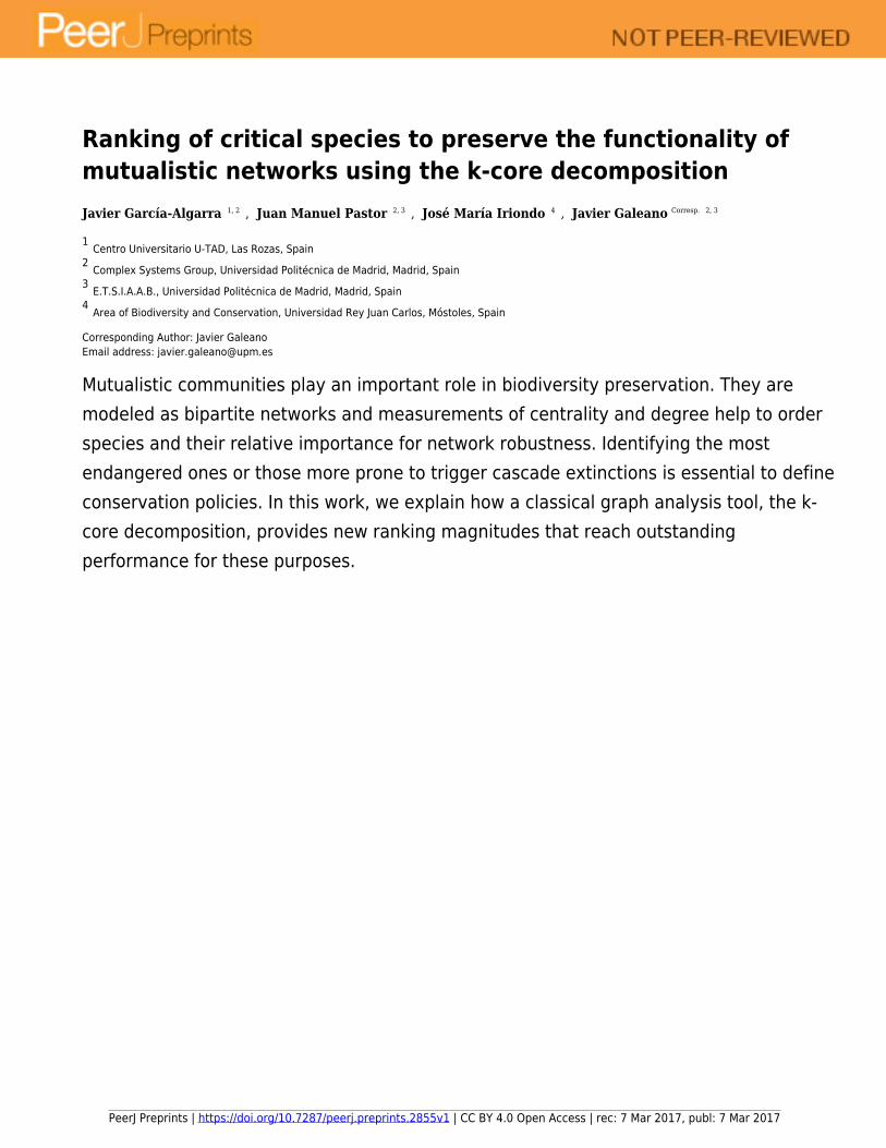
Ranking of critical species to preserve the functionality of

mutualistic networks using the k-core decomposition

Javier García-Algarra 1, 2 , Juan Manuel Pastor 2, 3 , José María Iriondo 4 , Javier Galeano Corresp. 2, 3

1 Centro Universitario U-TAD, Las Rozas, Spain2 Complex Systems Group, Universidad Politécnica de Madrid, Madrid, Spain3 E.T.S.I.A.A.B., Universidad Politécnica de Madrid, Madrid, Spain4 Area of Biodiversity and Conservation, Universidad Rey Juan Carlos, Móstoles, Spain

Corresponding Author: Javier Galeano

Email address: [email protected]

Mutualistic communities play an important role in biodiversity preservation. They are

modeled as bipartite networks and measurements of centrality and degree help to order

species and their relative importance for network robustness. Identifying the most

endangered ones or those more prone to trigger cascade extinctions is essential to define

conservation policies. In this work, we explain how a classical graph analysis tool, the k-

core decomposition, provides new ranking magnitudes that reach outstanding

performance for these purposes.

PeerJ Preprints | https://doi.org/10.7287/peerj.preprints.2855v1 | CC BY 4.0 Open Access | rec: 7 Mar 2017, publ: 7 Mar 2017

Ranking of critical species to preserve the1

functionality of mutualistic networks using2

the k-core decomposition3

Javier Garcıa-Algarra1,4, Juan Manuel Pastor1,2, Jose Marıa Iriondo3, and4

Javier Galeano1,25

1Complex Systems Group, Universidad Politecnica de Madrid, Madrid, Spain6

2E.T.S.I.A.A.B. , Dept. Ingenierıa Agroforestal, Universidad Politecnica de Madrid,7

Madrid, Spain8

3Area of Biodiversity and Conservation, Universidad Rey Juan Carlos, Mostoles, Spain9

4Centro Universitario U-TAD, Las Rozas, Spain10

Corresponding author:11

Javier Galeano112

Email address: [email protected]

ABSTRACT14

Mutualistic communities play an important role in biodiversity preservation. They are modeled as

bipartite networks and measurements of centrality and degree help to order species and their relative

importance for network robustness. Identifying the most endangered ones or those more prone to trigger

cascade extinctions is essential to define conservation policies. In this work, we explain how a classical

graph analysis tool, the k-core decomposition, provides new ranking magnitudes that reach outstanding

performance for these purposes.

15

16

17

18

19

20

INTRODUCTION21

Biotic interaction networks play an essential role in the stability of ecosystems (Tylianakis et al., 2010),22

as well as in the maintenance of biodiversity (Bascompte et al., 2006). Because community dynamics23

greatly depend on the way species interact, these networks have been described as the “biodiversity24

architecture” (Bascompte and Jordano, 2007). Network analysis has become an important approach25

to provide information on community organization and to predict dynamics and species extinctions in26

response to ecosystem disturbance (Tylianakis et al., 2010; Thebault and Fontaine, 2010; Traveset and27

Richardson, 2014). Among other assessments, these studies can point out key species, whose stability28

would prevent cascading extinctions, and the consequent loss of biodiversity (Sole and Montoya, 2001;29

Suweis et al., 2013; Dakos et al., 2014; Santamarıa et al., 2015). Research on cascading species extinctions30

as a result of perturbations in biotic interactions has tackled two main issues: the different ways to rank a31

hypothetical extinction sequence and the robustness and fragility measures (Pocock et al., 2012). There32

are different strategies both to sort species according to their importance and to measure their influence33

on extinction. For instance, in early studies on the resilience of food webs Dunne et al. ranked species by34

degree (i.e., the number of interactions) using three different scenarios of removal: a) from the species35

with the highest degree to the species with the lowest degree; b) from the lowest to the highest; c) species36

selected in a random way(Dunne et al., 2002). Memmott et al. worked the same idea to assess the37

robustness of mutualistic communities, removing active species and measuring the fraction of remaining38

passive species (Memmott et al., 2004).39

An observed property of mutualistic interactions is the existence of generalists, highly interconnected,40

and specialists, with few interactions linked to the generalists, but rarely among them. The nucleus41

of interactions among generalists seems to be the foundation of resilience. This property has been42

traditionally identified with nestedness (Bascompte et al., 2003), although there are new approaches to43

describe it in a more general way as a core-periphery organization (Csermely et al., 2013; Rombach et al.,44


2014).45

Identification of key nodes for community preservation is another active field of research. Besides46

classical measures of centrality, new rankings are available and provide efficient ways to find out them in47

bipartite networks (Tacchella et al., 2012; Domınguez-Garcıa and Munoz, 2015).48

In this paper, we aim to explain how the k-core decomposition, sheds light on the understanding49

of robustness in mutualism. The tool classifies the nodes of the network in shells, as in an onion-like50

structure with the most connected nodes in its center. Taking into account just the very basic topological51

properties, the decomposition helps to assess in detail the structure of mutualism and enlightens on the52

processes of species extinction cascades. Derived from the k-core decomposition we introduce three53

new magnitudes, hereafter called k-magnitudes, that describe network compactness (k-radius), combined54

quantity and quality of interactions (k-degree) and species vulnerability to trigger extinction cascades55

(k-risk). We assess the best criteria for identifying the species for which the networks are most vulnerable56

to cascade extinctions by comparing k-degree and k-risk ranking criteria with ranking by well-known57

indexes and applying them in two network destruction procedures. To conduct the test, we use one of the58

most complete available data sets (Fortuna et al., 2014).59

MATERIALS AND METHODS60

Data61

We have analyzed the Web of life collection (Fortuna et al., 2014), comprised by 89 mutualistic networks,62

with 59 communities of plants and pollinators and 30 of seed dispersers (http://www.web-of-life.63

es/). There are 57 communities with binary adjacency matrix (i.e., the interaction between the two64

species is recorded but not its strength), and 32 with weighted matrix, where the strength is accounted for.65

Network sizes range from 6 to 997 species, the minimum number of links is 6 and the maximum is 2933.66

Decomposition and k-magnitudes67

The idea of core decomposition was first described by Seidman to measure local density and cohesion68

in social graphs (Seidman, 1983). It has been successfully applied to visualize large systems and69

networks (Alvarez-Hamelin et al., 2005; Kitsak et al., 2010; Zhang et al., 2010; Barbera et al., 2015).70

The k-core of a network is a maximal connected sub-network of degree greater or equal than k. That71

means that each node is tied to at least k other nodes in the same sub-network.72

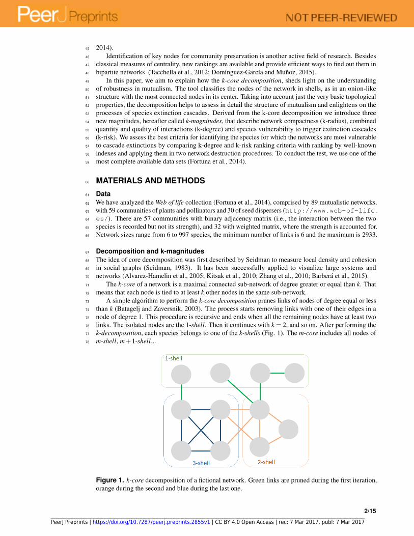
A simple algorithm to perform the k-core decomposition prunes links of nodes of degree equal or less73

than k (Batagelj and Zaversnik, 2003). The process starts removing links with one of their edges in a74

node of degree 1. This procedure is recursive and ends when all the remaining nodes have at least two75

links. The isolated nodes are the 1-shell. Then it continues with k = 2, and so on. After performing the76

k-decomposition, each species belongs to one of the k-shells (Fig. 1). The m-core includes all nodes of77

m-shell, m+1-shell...78

Figure 1. k-core decomposition of a fictional network. Green links are pruned during the first iteration,

orange during the second and blue during the last one.

2/15


Mutualistic networks are bipartite, with two guilds of species (plant-pollinator or plant-seed disperser79

in the studied collection). Links among nodes of the same class are forbidden. We will call these guilds A80

and B.81

Based on the k-core decomposition, we define three k-magnitudes. In order to quantify the distance82

from a node to the innermost shell of the partner guild, we define kradius. The kradius of node m of guild A83

is the average distance to all species of the innermost shell of guild B. We call this set NB.84

kAradius(m) =

1

| NB | ∑j∈NB

distm j m ∈ A (1)

where distm j is the shortest path from species m to each of the j species that belong to NB. The minimum85

possible kradius value is 1 for one node of the innermost shell directly linked to each one of the innermost86

shell set of the opposite guild.87

To obtain a measure of centrality in this k-shell based decomposition, we define kdegree as88

kAdegree (m) = ∑

j

am j

kBradius ( j)

m ∈ A,∀ j ∈ B (2)

where am j is the element of the interaction matrix that represents the link, considered as binary. If the89

network is weighted, am j will count as 1 for this purpose if there is interaction, 0 otherwise. kdegree(m) is90

a weighted degree where each node i linked to node m adds the inverse of its kradius(i). Generalists score91

high kdegree, whereas specialists, which have only one or two links, with similar kradius, score lower kdegree.92

This magnitude reminds the definition of the Harary index (Plavsic et al., 1993) but only considering93

paths from the nodes tied from m to the nodes of the innermost shell.94

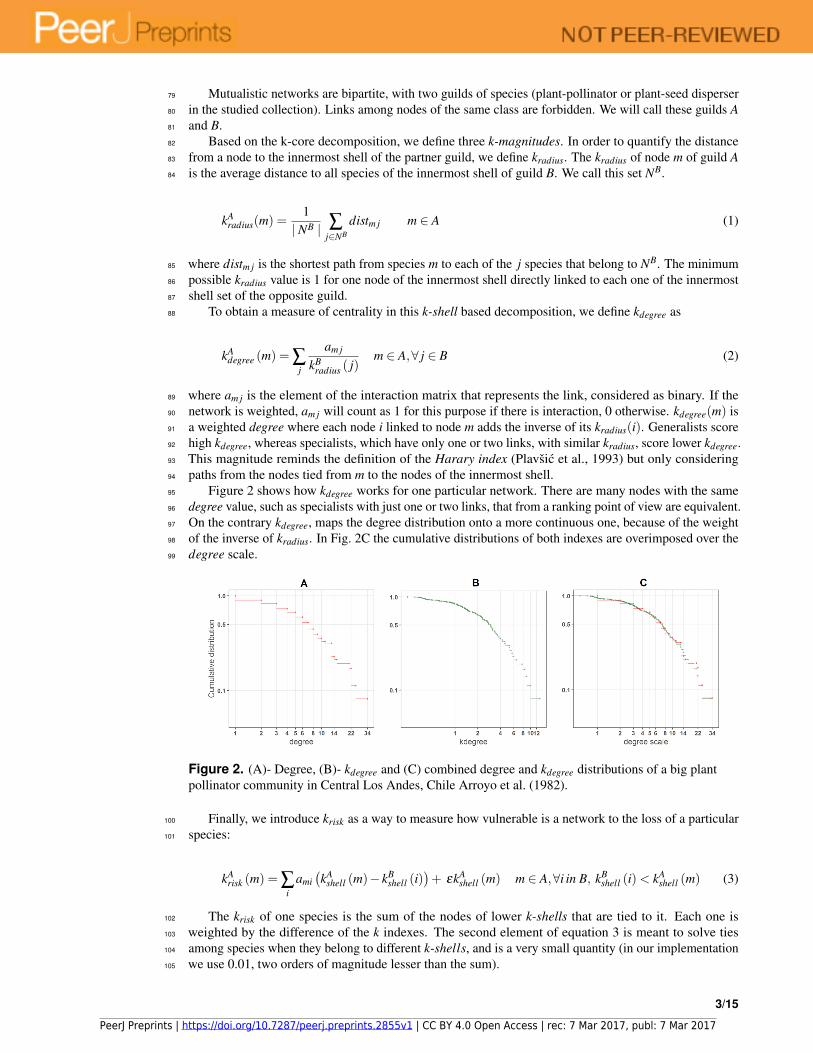
Figure 2 shows how kdegree works for one particular network. There are many nodes with the same95

degree value, such as specialists with just one or two links, that from a ranking point of view are equivalent.96

On the contrary kdegree, maps the degree distribution onto a more continuous one, because of the weight97

of the inverse of kradius. In Fig. 2C the cumulative distributions of both indexes are overimposed over the98

degree scale.99

Figure 2. (A)- Degree, (B)- kdegree and (C) combined degree and kdegree distributions of a big plant

pollinator community in Central Los Andes, Chile Arroyo et al. (1982).

Finally, we introduce krisk as a way to measure how vulnerable is a network to the loss of a particular100

species:101

kArisk (m) = ∑

i

ami

(

kAshell (m)− kB

shell (i))

+ εkAshell (m) m ∈ A,∀i in B, kB

shell (i)< kAshell (m) (3)

The krisk of one species is the sum of the nodes of lower k-shells that are tied to it. Each one is102

weighted by the difference of the k indexes. The second element of equation 3 is meant to solve ties103

among species when they belong to different k-shells, and is a very small quantity (in our implementation104

we use 0.01, two orders of magnitude lesser than the sum).105

3/15


In an intuitive way, if we remove one node strongly connected to others of lower k-shells, these species106

are in high risk of being dragged by the primary extinction. On the other hand, the extinction is much less107

dangerous for the species of higher k-shells linked to the same node, because they enjoy more redundant108

paths towards the network nucleus.109

Applying the k-magnitudes to a network110

Fig. 3 is an small seed disperser network with five species of plants, four species of thrushes and111

eleven links. We call, by convention, guild A the set of plants, and guild B the set of birds. The k-core112

decomposition was performed with the R igraph package (Csardi and Nepusz, 2006) . The maximum113

k index is 2. The four bird species belong to 2-shell; there are three plant species in 1-shell and two in114

2-shell. In this example each species of 2-shell is directly tied to all species of the opposite guild 2-shell,115

but this is not a general rule.116

Figure 3. Computation of the k-magnitudes. Seed disperser network in Santa Barbara, Sierra de Baza

(Spain) (Jordano, 1993). A: Decomposed network. B: Computing kBradius(4).

The shortest path from plant species 2 to each of the four bird species of 2-shell is 1, because of the117

direct links. So, kAradius(2) is 1. The same reasoning is valid for plant species 1. The reader may check that118

the kradius of bird species of 2-shell is 1 as well, measuring their shortest paths to plants species 1 and 2.119

Computation of this magnitude is simple although a bit more laborious for 1-shell plant species. We120

work plant species 4 as an example. First, we find the shortest paths to each bird species of 2-shell.121

Shortest paths are depicted with different colors. Plant species 4 is tied to seed disperser species 1, so122

distance is 1. On the other hand, there is no direct link with bird species 2. Shortest path is pl4-disp1-123

pl2-disp2, and distance is 3. It is easy to check that distances from plant species 4 to bird species 3 and 4124

are also 3. Once we have found the four distances, we compute kBradius (4) as the average of 1, 3, 3 and 3,125

that is 2.5.126

The values of kdegree are straightforward to compute. For instance, the kdegree of disperser species 1 is:127

kBdegree (1) =

1

kAradius (1)

+1

kAradius (2)

+1

kAradius (4)

+1

kAradius (5)

= 2.8 (4)

The last k-magnitude we defined was krisk. We use again the disperser species 1 as example. Links to

species of the same or upper k-shells are irrelevant to compute krisk, so only bird species 4 and 5 are taken

into account.

kBrisk (1) = kB

shell (1)−kAshell (4)+kB

shell (1)−kAshell (5)+εkB

shell (1) = (2−1)+(2−1)+0.01x2= 2.02 (5)

This magnitude may seem counter-intuitive, because the krisk of a highly connected species like plant128

1 is 0.02, almost the same of that of peripheral plant 3. This is because plant 1 has no ties with lower129

k-shell animal species. The krisk ranks species to assess resilience, it has not an absolute meaning. It just130

tells us that it is more dangerous for the network to remove the disperser 1 than plant 1, and plant 1 than131

plant 3.132

The k-magnitudes of the example network are shown in table 1.133

4/15


Species kshell kradius kdegree krisk

pl1 2 1 4 0.02

pl2 2 1 4 0.02

pl3 1 2.5 1 0.01

pl4 1 2.5 1 0.01

pl5 1 2.5 1 0.01

disp1 2 1 2.8 2.02

disp2 2 1 2.4 1.02

disp3 2 1 2 0.02

disp4 2 1 2 0.02

Table 1. K-magnitudes of the network of Fig. 3.

Extinction procedures134

We carried out two static extinction procedures. Static assumption implies that there is not rewiring (e.g.,135

plants that have lost their pollinators are not pollinated by other insects) , despite this kind of network136

reorganization is observed in nature (Ramos-Jiliberto et al., 2012; Goldstein and Zych, 2016; Timoteo137

et al., 2016). Nodes are ranked once, before the procedure starts.138

In the first method, one species is removed each step, in decreasing order according to the chosen139

index, no matter to which guild it belongs. Four ranking indexes are compared: krisk, kdegree, degree140

and eigenvector centrality. The k indexes were computed with the R package kcorebip; degree and141

eigenvector centrality with the degree and evcent functions of the igraph package.142

To estimate the damage caused to the network, the fraction of remaining giant component (i.e., the143

highest connected component of a given network) was used. The procedure stops when this ratio is equal144

or less than 0.5. To break ties, we ran 100 experiments for each network and index, shuffling species with145

the same ranking value. The percentage of removed species needed to get to 0.5 of the remaining giant146

component is used to measure the performance of the ranking. The lower the percentage of removed147

species, the more efficient the ranking is in destroying the network. The top performer scores the least148

average removal percentage. (Fig. 4).149

Figure 4. First extinction procedure. Performance of the four ranking indexes for a pollinator

community described by Elberling and Olesen in Zackenberg Station (Greenland, unpublished).

Individual dots are the results of each experiment while black dots are the average values

.

The second extinction procedure that we followed is more common in the literature. Only animal150

species are actively removed (primary extinctions); secondary extinctions happen when nodes become151

isolated (Memmott et al., 2004).152

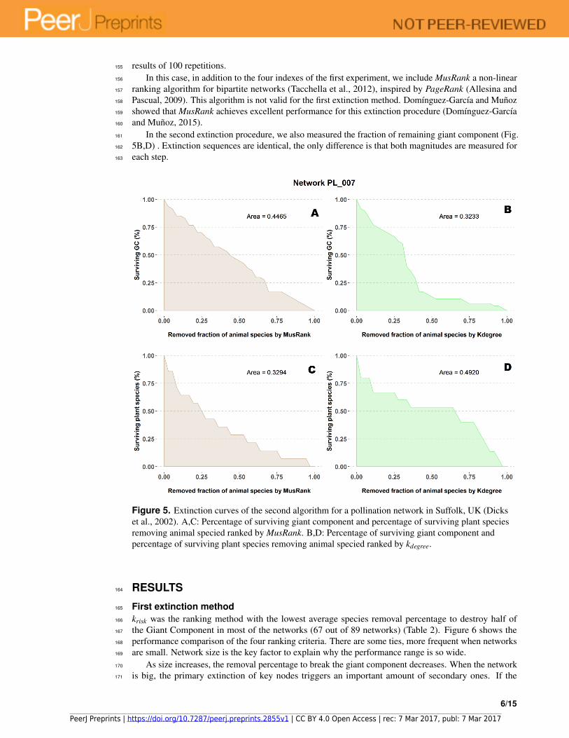
The fraction of surviving plant species is measured as a function of the removed fraction of animal153

species (Fig. 5A,C) and the area under the curve is the value to compare performance. We averaged the154

5/15


results of 100 repetitions.155

In this case, in addition to the four indexes of the first experiment, we include MusRank a non-linear156

ranking algorithm for bipartite networks (Tacchella et al., 2012), inspired by PageRank (Allesina and157

Pascual, 2009). This algorithm is not valid for the first extinction method. Domınguez-Garcıa and Munoz158

showed that MusRank achieves excellent performance for this extinction procedure (Domınguez-Garcıa159

and Munoz, 2015).160

In the second extinction procedure, we also measured the fraction of remaining giant component (Fig.161

5B,D) . Extinction sequences are identical, the only difference is that both magnitudes are measured for162

each step.163

Figure 5. Extinction curves of the second algorithm for a pollination network in Suffolk, UK (Dicks

et al., 2002). A,C: Percentage of surviving giant component and percentage of surviving plant species

removing animal specied ranked by MusRank. B,D: Percentage of surviving giant component and

percentage of surviving plant species removing animal specied ranked by kdegree.

RESULTS164

First extinction method165

krisk was the ranking method with the lowest average species removal percentage to destroy half of166

the Giant Component in most of the networks (67 out of 89 networks) (Table 2). Figure 6 shows the167

performance comparison of the four ranking criteria. There are some ties, more frequent when networks168

are small. Network size is the key factor to explain why the performance range is so wide.169

As size increases, the removal percentage to break the giant component decreases. When the network170

is big, the primary extinction of key nodes triggers an important amount of secondary ones. If the171

6/15


community has 100 or more species, krisk is even a better predictor of the most damaging extinction172

sequence and outperforms the other indexes for 28 out of 32 networks.173

Table 2. Average number of removed species to destroy half the Giant Component, according to the

different indexes: krisk is the top performer for 67 networks, degree for 48, kdegree for 39 and eigenvector

centrality for 28 networks.

Network GCsize krisk degree kdegree eigen Network GCsize krisk degree kdegree eigen

PL 001 177 21.73 22.13 22 23 PL 046 60 11 11.94 13 14PL 002 103 14.46 12.51 13 15 PL 047 205 4 4 4 4PL 003 61 5 5.35 6 6 PL 048 266 10 10 9 12PL 004 112 3 3 3 3 PL 049 262 11 13 15 16PL 005 361 25 30.73 36 42 PL 050 49 6 6.36 7 7PL 006 78 3 3 3 3 PL 051 104 3 3 3 3PL 007 50 5 4 4 4 PL 052 52 6 6 6 7PL 008 49 6 7 7 11 PL 053 364 19 22.49 23 34PL 009 142 7 7.52 8 12 PL 054 414 23 25.23 27 30PL 010 107 23.46 29 29 32 PL 055 253 16.40 17 19PL 011 27 4 5.04 6 6 PL 056 456 22 28.71 33 43PL 012 84 7 7 7 7 PL 057 997 17 17 20 36PL 013 65 4 4 4 5 PL 058 111 14 17.55 19 20PL 014 108 6 5 5 6 PL 059 26 6 5 5 5PL 015 793 48 56 60 87 SD 001 28 3 3 3 5PL 016 205 9 9 10 17 SD 002 40 5 5 5 5PL 017 104 9 10.52 11 11 SD 003 41 4 4 4 4PL 018 144 18 19 23 24 SD 004 52 4 4 4 4PL 019 123 14 15.37 16 18 SD 005 34 3 3 3 3PL 020 109 3 3 3 3 SD 006 34 4 4.31 5 5PL 021 766 12 12 12 38 SD 007 79 3 3 3 3PL 022 66 4 4 4 4 SD 008 26 9.83 8.45 8 11PL 023 90 3 3 3 3 SD 009 25 3 4 4 5PL 024 22 4 3.55 3 3.0 SD 010 64 8 8 9 13PL 025 57 6 6 6 10 SD 011 25 6 5.33 5 6PL 026 150 2 2 2 2 SD 012 64 12.71 12.53 12 14PL 027 75 8.54 8 9 11 SD 013 55 11 8 19 14PL 028 180 13 14 16 24 SD 014 33 9 10 10 10PL 029 167 17 16.97 17 19 SD 015 32 4 4 4 4PL 030 70 10.23 6.65 7 13 SD 016 85 17 18 20 23PL 031 91 9.53 7.92 13 17 SD 017 24 7.28 6.62 10 10PL 032 40 2 2 2 2 SD 018 53 5 5 5 5PL 033 47 8.65 8 10 12 SD 019 209 13 16.48 20 21PL 034 151 6 7.54 8 9 SD 020 58 7.65 9.22 10 10PL 035 97 6 7.54 8 9 SD 021 46 9 10 10 10PL 036 22 3.68 2 2 2 SD 022 317 39 50.43 53 60PL 037 50 5 5 5 7 SD 023 23 4 4 4 4PL 038 50 4 4 4 7 SD 024 19 6 6 7 8PL 039 68 6 6.68 9 10 SD 025 13 4.38 4.16 4.16 4PL 040 70 8.56 7 9 10 SD 026 6 2 2 2 2PL 041 70 10 10 11 12 SD 027 16 3 3 3 3PL 042 16 2 2 2 2 SD 028 13 3 3 3 3PL 043 110 12 14 14 19 SD 029 9 2 2 2 2PL 044 712 21 23 25 49 SD 030 9 2 2.65 2 2PL 045 41 6 5.45 7 8

7/15


Figure 6. First extinction method. The average percentage of removed species to destroy the Giant

Component is depicted for each network and ranking index. Under the X axis, the name of each network

as coded in the web of life database. The overall top performer is krisk (see Table 2). Species are ordered

by the percentage of primary extinctions, ranked by krisk . The red line joins the krisk destruction

percentage values as a visual reference to compare them with those of the other indexes.

8/15


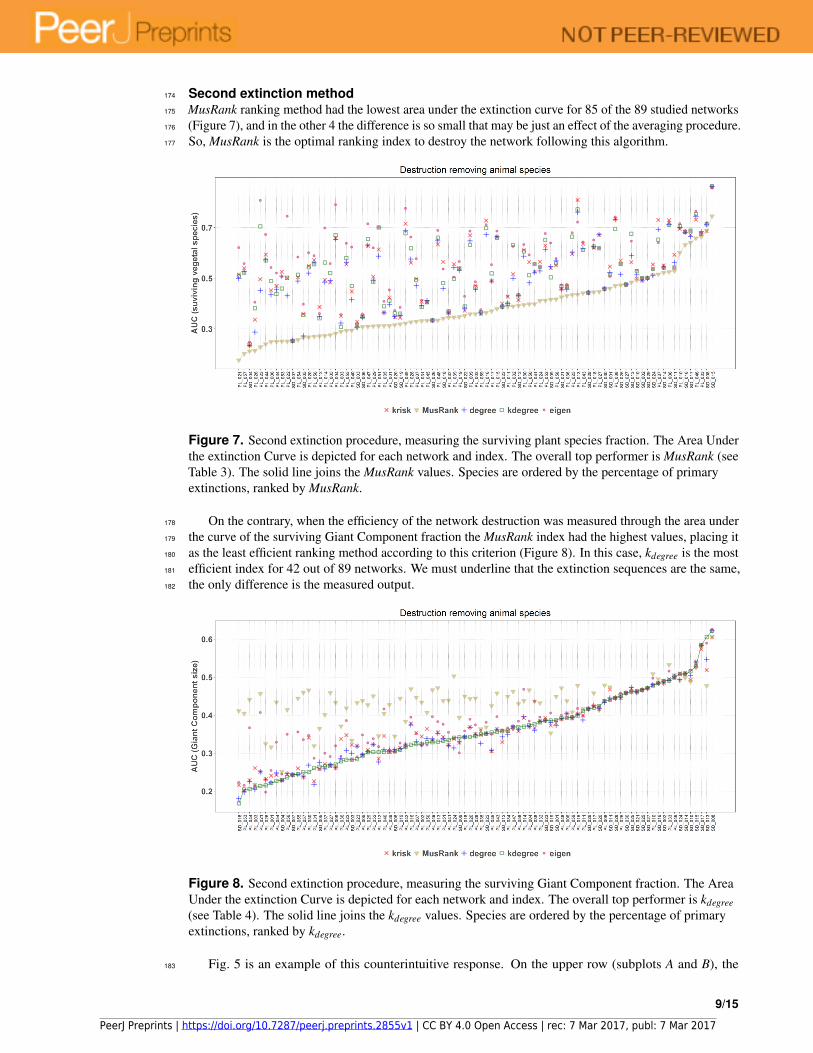
Second extinction method174

MusRank ranking method had the lowest area under the extinction curve for 85 of the 89 studied networks175

(Figure 7), and in the other 4 the difference is so small that may be just an effect of the averaging procedure.176

So, MusRank is the optimal ranking index to destroy the network following this algorithm.177

Figure 7. Second extinction procedure, measuring the surviving plant species fraction. The Area Under

the extinction Curve is depicted for each network and index. The overall top performer is MusRank (see

Table 3). The solid line joins the MusRank values. Species are ordered by the percentage of primary

extinctions, ranked by MusRank.

On the contrary, when the efficiency of the network destruction was measured through the area under178

the curve of the surviving Giant Component fraction the MusRank index had the highest values, placing it179

as the least efficient ranking method according to this criterion (Figure 8). In this case, kdegree is the most180

efficient index for 42 out of 89 networks. We must underline that the extinction sequences are the same,181

the only difference is the measured output.182

Figure 8. Second extinction procedure, measuring the surviving Giant Component fraction. The Area

Under the extinction Curve is depicted for each network and index. The overall top performer is kdegree

(see Table 4). The solid line joins the kdegree values. Species are ordered by the percentage of primary

extinctions, ranked by kdegree.

Fig. 5 is an example of this counterintuitive response. On the upper row (subplots A and B), the183

9/15


difference for both ranking indexes when measuring the giant component. While this magnitude decreases184

at a constant pace for MusRank, there is a sharp reduction of the component size when one third of animal185

species are removed following the kdegree ranking. On the lower row (subplots C and D), opposite results186

are obtained when accounting for the fraction of surviving plant species.187

Figure 9. Pollinator network 007 (Dicks et al., 2002). A: Original configuration; B: Structure after the

removal of the 13 top MusRank-ranked animal species. C: Structure after the removal of the 13 top

kdegree-ranked animal species

The destruction of this pollinator network sheds light on the root cause of the difference. The network188

has 36 pollinator and 16 plant species (Fig.9A), 2 of them are outside the giant component. When the 13189

top animal species ranked by MusRank are removed (pollinators 3,1,7,15,32,6,14,33,13,31,8,16,10),190

the community reaches the degraded structure of Fig.9B. The size of the giant component is 27 (54% of191

the original), and there are 23 pollinator and 6 plant species.192

If we remove the 13 top animal species ranked by kdegree (pollinators 1,3,7,13,15,2,11,20,12,8,6,5,10)193

instead, the community structure is that of Fig.9C. Now, the size of the giant component is 19 (38% of the194

original), and there are 23 pollinator and 9 plant species. MusRank has killed more plant species, but the195

giant component is clearly smaller ranking by kdegree.196

10/15


Table 3. Average area under the extinction curve, when the surviving fraction of plant species is

measured. MusRank is the top performer for 85 networks , krisk for 9, degree for 8, kdegree for 7 and

eigenvector centrality for 7.

Net

work

MR

k ris

kk d

egre

edeg

ree

eigen

vN

etw

ork

MR

k ris

kk d

egre

edeg

ree

eigen

v

PL

001

0.3

121

0.4

236

0.4

115

0.3

956

0.4

535

PL

046

0.6

577

0.7

308

0.7

528

0.7

445

0.7

642

PL

002

0.3

588

0.4

710

0.4

641

0.4

555

0.4

856

PL

047

0.3

091

0.6

283

0.6

541

0.6

302

0.7

143

PL

003

0.2

896

0.3

505

0.3

085

0.3

232

0.3

563

PL

048

0.3

336

0.6

334

0.6

594

0.6

471

0.6

887

PL

004

0.2

821

0.6

579

0.6

695

0.6

536

0.7

900

PL

049

0.3

220

0.7

150

0.6

773

0.6

880

0.7

757

PL

005

0.2

755

0.4

836

0.5

198

0.4

906

0.5

573

PL

050

0.3

976

0.5

635

0.5

114

0.4

815

0.5

918

PL

006

0.2

490

0.4

520

0.4

882

0.4

344

0.5

420

PL

051

0.3

115

0.6

132

0.7

000

0.5

870

0.7

008

PL

007

0.3

294

0.4

982

0.4

920

0.4

702

0.5

769

PL

052

0.4

121

0.6

289

0.6

514

0.6

132

0.6

761

PL

008

0.5

251

0.7

287

0.7

093

0.7

117

0.7

213

PL

053

0.2

510

0.5

253

0.4

590

0.5

081

0.5

058

PL

009

0.3

583

0.6

689

0.6

315

0.6

473

0.6

857

PL

054

0.2

568

0.5

035

0.5

136

0.4

885

0.5

835

PL

010

0.6

004

0.6

948

0.7

044

0.7

003

0.7

150

PL

055

0.2

929

0.5

548

0.5

795

0.5

633

0.6

378

PL

011

0.3

876

0.4

272

0.3

994

0.3

999

0.4

290

PL

056

0.2

696

0.5

717

0.5

545

0.5

605

0.5

885

PL

012

0.2

716

0.3

860

0.3

417

0.3

494

0.3

604

PL

057

0.2

019

0.5

392

0.5

217

0.5

261

0.5

576

PL

013

0.4

353

0.8

088

0.7

716

0.7

606

0.7

212

PL

058

0.4

168

0.5

507

0.5

585

0.5

683

0.5

773

PL

014

0.2

726

0.4

935

0.5

617

0.4

840

0.6

980

PL

059

0.3

639

0.3

587

0.3

649

0.3

631

0.3

757

PL

015

0.3

792

0.6

637

0.6

579

0.6

633

0.6

859

SD

001

0.4

592

0.5

459

0.5

141

0.5

229

0.5

068

PL

016

0.3

641

0.7

275

0.6

973

0.6

719

0.7

108

SD

002

0.5

000

0.4

911

0.5

000

0.4

919

0.5

000

PL

017

0.3

703

0.4

895

0.5

187

0.4

886

0.5

532

SD

003

0.3

051

0.3

281

0.3

166

0.3

059

0.3

166

PL

018

0.4

451

0.6

194

0.6

249

0.6

259

0.6

504

SD

004

0.2

121

0.2

351

0.2

389

0.2

350

0.2

476

PL

019

0.3

474

0.5

391

0.5

373

0.5

320

0.5

658

SD

005

0.2

656

0.3

587

0.3

546

0.2

718

0.3

974

PL

020

0.2

674

0.5

480

0.5

427

0.5

199

0.6

005

SD

006

0.3

078

0.3

515

0.3

471

0.3

444

0.3

588

PL

021

0.1

761

0.5

147

0.5

092

0.4

985

0.6

207

SD

007

0.2

528

0.2

528

0.2

528

0.2

528

0.2

528

PL

022

0.2

511

0.5

003

0.5

019

0.4

304

0.7

444

SD

008

0.6

875

0.6

861

0.7

125

0.7

108

0.7

188

PL

023

0.2

285

0.4

959

0.7

041

0.4

517

0.8

068

SD

009

0.4

167

0.5

395

0.5

033

0.5

453

0.6

389

PL

024

0.4

111

0.5

650

0.5

449

0.5

283

0.5

444

SD

010

0.4

929

0.4

986

0.5

271

0.5

129

0.5

314

PL

025

0.4

344

0.5

956

0.6

641

0.6

030

0.6

792

SD

011

0.5

286

0.5

927

0.5

422

0.5

623

0.5

422

PL

026

0.2

138

0.3

362

0.3

811

0.2

874

0.4

052

SD

012

0.3

912

0.4

140

0.4

321

0.4

316

0.4

332

PL

027

0.4

466

0.6

711

0.6

179

0.6

728

0.6

185

SD

013

0.4

835

0.5

629

0.6

754

0.5

885

0.6

462

PL

028

0.3

266

0.5

613

0.6

178

0.5

754

0.6

621

SD

014

0.5

221

0.5

504

0.5

415

0.5

441

0.5

404

PL

029

0.3

107

0.5

061

0.4

865

0.4

919

0.6

198

SD

015

0.7

444

0.8

602

0.8

633

0.8

607

0.8

556

PL

030

0.3

949

0.6

113

0.6

054

0.5

870

0.6

329

SD

016

0.6

318

0.6

812

0.6

830

0.6

816

0.6

872

PL

031

0.3

314

0.4

078

0.3

857

0.3

926

0.4

128

SD

017

0.6

406

0.6

719

0.6

875

0.6

639

0.6

875

PL

032

0.3

889

0.5

157

0.6

312

0.4

995

0.6

255

SD

018

0.3

413

0.5

645

0.4

809

0.4

596

0.5

361

PL

033

0.6

640

0.6

732

0.6

753

0.6

832

0.6

799

SD

019

0.3

185

0.3

444

0.3

602

0.3

535

0.3

849

PL

034

0.2

497

0.4

697

0.4

383

0.4

563

0.5

204

SD

020

0.3

155

0.3

459

0.3

608

0.3

485

0.3

722

PL

035

0.3

121

0.3

648

0.3

886

0.3

633

0.4

085

SD

021

0.4

254

0.4

579

0.4

682

0.4

567

0.4

737

PL

036

0.4

306

0.4

677

0.4

667

0.4

560

0.4

750

SD

022

0.3

517

0.3

720

0.3

886

0.3

820

0.4

284

PL

037

0.5

153

0.7

303

0.6

521

0.6

924

0.6

400

SD

023

0.3

875

0.4

000

0.3

875

0.3

875

0.3

875

PL

038

0.4

702

0.7

328

0.6

948

0.7

310

0.7

411

SD

024

0.5

130

0.5

542

0.5

357

0.5

114

0.5

357

PL

039

0.3

454

0.5

556

0.4

979

0.5

425

0.5

046

SD

025

0.4

722

0.5

692

0.5

556

0.5

156

0.5

556

PL

040

0.2

940

0.4

478

0.4

696

0.4

153

0.6

227

SD

026

0.3

333

0.3

333

0.3

333

0.3

333

0.3

333

PL

041

0.3

978

0.5

253

0.5

562

0.5

238

0.5

566

SD

027

0.4

750

0.4

750

0.4

750

0.4

750

0.4

750

PL

042

0.3

452

0.3

621

0.3

690

0.3

621

0.3

690

SD

028

0.4

429

0.4

429

0.4

429

0.4

429

0.4

429

PL

043

0.4

414

0.6

364

0.6

113

0.6

183

0.6

430

SD

029

0.5

000

0.5

000

0.5

000

0.5

000

0.5

000

PL

044

0.2

401

0.5

932

0.5

701

0.5

723

0.6

721

SD

030

0.4

583

0.4

583

0.4

583

0.4

583

0.4

583

PL

045

0.3

324

0.4

052

0.4

047

0.4

116

0.4

063

11/15


Table 4. Average area under the extinction curve, when the surviving fraction of the original giant

component is measured. The top performer is kdegree for 42 networks, degree for 24, krisk for 21,

eigenvector centrality for 18 and MusRank for 16.

Net

work

MusR

ank

k ris

kk d

egre

edeg

ree

eigen

vN

etw

ork

MusR

ank

k ris

kk d

egre

edeg

ree

eigen

v

PL

001

0.3

158

0.2

410

0.2

212

0.2

224

0.2

546

PL

046

0.5

060

0.4

975

0.5

013

0.5

008

0.4

987

PL

002

0.4

337

0.3

441

0.3

244

0.3

237

0.3

198

PL

047

0.4

626

0.3

694

0.3

686

0.3

694

0.3

622

PL

003

0.2

176

0.2

607

0.2

093

0.2

056

0.2

145

PL

048

0.4

715

0.3

895

0.3

920

0.3

909

0.3

998

PL

004

0.4

661

0.3

700

0.3

744

0.3

697

0.3

843

PL

049

0.4

662

0.3

350

0.3

286

0.3

372

0.3

960

PL

005

0.4

380

0.2

954

0.2

935

0.2

968

0.3

482

PL

050

0.4

068

0.3

641

0.3

285

0.3

387

0.3

214

PL

006

0.4

374

0.4

044

0.3

929

0.4

038

0.3

932

PL

051

0.4

380

0.3

428

0.3

322

0.3

384

0.3

762

PL

007

0.4

465

0.3

539

0.3

233

0.3

310

0.3

513

PL

052

0.4

502

0.3

228

0.3

029

0.3

227

0.3

381

PL

008

0.4

786

0.4

363

0.4

370

0.4

344

0.4

386

PL

053

0.4

046

0.2

018

0.2

045

0.1

980

0.2

153

PL

009

0.4

331

0.2

613

0.2

703

0.2

617

0.3

195

PL

054

0.4

337

0.2

427

0.2

273

0.2

481

0.3

287

PL

010

0.5

086

0.4

789

0.4

783

0.4

802

0.4

974

PL

055

0.4

443

0.2

602

0.2

449

0.2

443

0.3

557

PL

011

0.4

169

0.3

994

0.4

108

0.3

874

0.3

985

PL

056

0.4

142

0.2

451

0.2

364

0.2

460

0.3

498

PL

012

0.3

451

0.2

859

0.3

030

0.2

768

0.3

173

PL

057

0.4

597

0.2

378

0.2

498

0.2

377

0.3

355

PL

013

0.4

718

0.3

548

0.3

302

0.3

527

0.3

828

PL

058

0.4

301

0.3

578

0.3

694

0.3

622

0.3

840

PL

014

0.4

378

0.3

928

0.3

697

0.3

965

0.4

679

PL

059

0.4

077

0.3

916

0.3

944

0.3

934

0.3

954

PL

015

0.4

780

0.4

030

0.3

991

0.4

025

0.4

177

SD

001

0.4

489

0.3

792

0.3

871

0.3

732

0.3

854

PL

016

0.4

689

0.3

781

0.3

221

0.3

743

0.3

946

SD

002

0.4

905

0.4

849

0.4

905

0.4

847

0.4

905

PL

017

0.4

579

0.4

240

0.4

190

0.4

257

0.4

234

SD

003

0.3

333

0.3

222

0.2

829

0.2

999

0.2

829

PL

018

0.4

498

0.3

419

0.3

421

0.3

432

0.3

585

SD

004

0.2

510

0.2

286

0.2

298

0.2

288

0.2

448

PL

019

0.4

441

0.3

138

0.3

083

0.3

118

0.3

265

SD

005

0.3

646

0.2

592

0.2

640

0.2

762

0.2

569

PL

020

0.4

433

0.3

688

0.3

426

0.3

674

0.3

894

SD

006

0.3

444

0.3

072

0.3

049

0.3

088

0.3

025

PL

021

0.4

563

0.2

512

0.2

136

0.2

510

0.4

071

SD

007

0.2

433

0.2

433

0.2

433

0.2

433

0.2

433

PL

022

0.4

184

0.3

475

0.2

828

0.3

068

0.3

858

SD

008

0.6

060

0.6

056

0.6

220

0.6

221

0.6

260

PL

023

0.4

327

0.3

187

0.2

840

0.3

185

0.2

901

SD

009

0.3

935

0.3

280

0.3

415

0.3

296

0.3

009

PL

024

0.5

028

0.3

380

0.3

406

0.3

135

0.3

389

SD

010

0.4

881

0.4

926

0.5

153

0.5

040

0.5

187

PL

025

0.4

529

0.4

451

0.4

521

0.4

472

0.4

582

SD

011

0.4

736

0.4

678

0.4

405

0.4

452

0.4

405

PL

026

0.3

245

0.2

316

0.2

153

0.2

300

0.1

976

SD

012

0.3

603

0.3

291

0.3

575

0.3

429

0.3

609

PL

027

0.4

590

0.2

669

0.2

676

0.2

698

0.2

912

SD

013

0.4

772

0.5

185

0.6

053

0.5

466

0.5

897

PL

028

0.4

445

0.3

505

0.3

444

0.3

483

0.3

743

SD

014

0.4

982

0.5

117

0.5

081

0.5

092

0.5

074

PL

029

0.4

270

0.3

084

0.3

024

0.3

040

0.3

272

SD

015

0.5

251

0.5

392

0.5

288

0.5

397

0.5

299

PL

030

0.4

658

0.3

410

0.2

504

0.2

685

0.3

469

SD

016

0.4

949

0.4

832

0.4

849

0.4

833

0.4

852

PL

031

0.3

190

0.2

263

0.2

603

0.2

178

0.2

866

SD

017

0.5

842

0.5

734

0.5

842

0.5

832

0.5

842

PL

032

0.4

322

0.3

853

0.3

810

0.3

831

0.3

951

SD

018

0.4

112

0.2

159

0.1

678

0.1

806

0.2

231

PL

033

0.5

326

0.4

953

0.4

910

0.4

914

0.5

160

SD

019

0.3

528

0.3

729

0.3

861

0.3

807

0.4

058

PL

034

0.4

489

0.3

585

0.3

596

0.3

497

0.3

664

SD

020

0.4

135

0.4

156

0.4

236

0.4

169

0.4

229

PL

035

0.3

636

0.3

488

0.3

498

0.3

259

0.3

595

SD

021

0.4

594

0.4

617

0.4

627

0.4

610

0.4

627

PL

036

0.3

708

0.3

377

0.2

785

0.2

859

0.2

917

SD

022

0.3

681

0.3

525

0.3

508

0.3

522

0.3

814

PL

037

0.4

010

0.2

716

0.2

652

0.2

585

0.2

997

SD

023

0.3

860

0.3

934

0.3

860

0.3

860

0.3

860

PL

038

0.4

366

0.3

665

0.3

767

0.3

605

0.4

366

SD

024

0.4

916

0.5

098

0.5

079

0.4

931

0.5

079

PL

039

0.4

274

0.3

036

0.3

042

0.3

080

0.3

083

SD

025

0.4

621

0.4

702

0.4

621

0.4

732

0.4

621

PL

040

0.4

042

0.3

454

0.3

037

0.3

096

0.4

164

SD

026

0.4

167

0.4

167

0.4

167

0.4

167

0.4

167

PL

041

0.4

394

0.3

216

0.3

344

0.3

205

0.3

550

SD

027

0.4

712

0.4

712

0.4

712

0.4

712

0.4

712

PL

042

0.3

833

0.3

227

0.3

167

0.3

218

0.3

167

SD

028

0.4

455

0.4

455

0.4

455

0.4

455

0.4

455

PL

043

0.4

577

0.3

634

0.3

558

0.3

616

0.3

959

SD

029

0.4

667

0.4

667

0.4

667

0.4

667

0.4

667

PL

044

0.4

410

0.2

286

0.2

058

0.2

255

0.3

669

SD

030

0.4

583

0.4

583

0.4

583

0.4

583

0.4

583

PL

045

0.4

246

0.3

052

0.3

544

0.3

066

0.3

496

12/15


DISCUSSION197

The k-core decomposition offers a new topological view of the structure of mutualistic networks. We have198

defined three new magnitudes to take advantage of their properties. Network compactness is described199

by kradius, a measure of average proximity to top generalists of the partner guild. Second, kdegree maps200

each node’s degree onto a finer grain distribution. It has not only information on the number of neighbors201

but also on how they are connected to the innermost shell. Finally, krisk is set to identify species whose202

disappearance poses a greater risk to the entire network.203

Comparing the k-magnitudes based extinction indexes (kdegree and krisk) with those routinely used204

when extinctions take place in both guilds, krisk is the best rank if the goal is to identify the key species to205

preserve most of the giant component. krisk identifies species linked to a high number of nodes of lower206

k-shells. These species provide vulnerability to the network because their extinction may drag many of207

the species with lower k-shells they are linked to, to extinction as well, as they do not enjoy redundant208

paths to the innermost shell.209

Applying the well-known method of removing species of the primary class and measuring the210

extinctions in secondary class, the most effective extinction sequence, if the goal is to identify the key211

species to preserve most of the giant component, is kdegree. However, if the goal is to identify the key212

species to preserve the greatest species richness in the second class (e.g., plants in a plant-pollinator213

mutualistic network), the best criterion is MusRank as Fig. 7 makes clear . These results confirm those214

obtained by Domınguez-Garcıa and Munoz (2015), over a larger network collection (89 in this work vs.215

67 in the original paper).216

The most striking result of the second method is how different performance is for a same ranking217

index, depending on the magnitude we measure. The root cause lies on the definitions of the indexes218

themselves. MusRank is optimal to destroy the plant guild. It identifies the most important active nodes of219

the bipartite network because of how they are linked to the most vulnerable passive ones. It was designed220

to excel with this extinction sequence and works with local properties. On the other hand, kdegree is an221

excellent performer to destroy the giant component. It contains information on how nodes are connected222

to the innermost shell, and ranks higher those nodes strongly tied to that stable nucleus.223

In summary, in this study, we show that the new k-core decomposition derived indexes, krisk and224

kdegree provide a new insight into the structure of mutualistic networks. This insight is particularly useful225

because these indexes fair much better than other traditionally used ranking indexes, when the aim is to226

identify the species that are key to preserving the interactions and the functionality of the community.227

As complex network studies on mutualistic interactions are already being used to suggest conservation228

policies, it is of utmost importance to have a clear framework of what the conservation practitioners look229

for when implementing conservation and restoration plans. The static view of considering biodiversity230

conservation as the mere conservation of a list of species has long been substituted by a new paradigm231

which looks at conservation from a dynamic viewpoint in which species interactions and the functionality232

of the ecosystems play a major role (Heywood and Iriondo, 2003).233

ADDITIONAL INFORMATION AND DECLARATIONS234

Funding235

This work was partially supported by the Ministry of Economy and Competitiveness of Spain. The funder236

was not involved in the study design.237

Grant Disclosures238

The following grant information was disclosed by the authors: MTM2012-39101, MTM2015-63914-P.239

Competing Interests240

The authors declare no competing interests.241

Author Contributions242

J.G-A., J.M.P and J.G. developed the mathematical analysis. J.G-A. wrote the R code and J.M.P. the243

Python code and they both performed simulations. J.M.I. provided advice in the overall design of the244

work and ecological interpretation of results. All authors wrote the paper.245

13/15


Code246

The R code for k-core decomposition and plotting has been published as a package at https://www.247

github.com/jgalgarra/kcorebip.248

The rest of software is available at https://github.com/jgalgarra/kcore_robustness249

Reproducibility instructions are detailed in the README.md file250

REFERENCES251

Allesina, S. and Pascual, M. (2009). Googling food webs: can an eigenvector measure species’ importance252

for coextinctions? PLoS Comput Biol, 5(9):e1000494.253

Alvarez-Hamelin, J. I., Dall’Asta, L., Barrat, A., and Vespignani, A. (2005). k-core decomposition: A254

tool for the visualization of large scale networks. arXiv preprint cs/0504107.255

Arroyo, M. T. K., Primack, R., and Armesto, J. (1982). Community studies in pollination ecology in the256

high temperate andes of central chile. i. pollination mechanisms and altitudinal variation. American257

journal of botany, pages 82–97.258

Barbera, P., Wang, N., Bonneau, R., Jost, J. T., Nagler, J., Tucker, J., and Gonzalez-Bailon, S. (2015). The259

critical periphery in the growth of social protests. PloS One, 10(11).260

Bascompte, J. and Jordano, P. (2007). Plant-animal mutualistic networks: the architecture of biodiversity.261

Annual Review of Ecology, Evolution, and Systematics, pages 567–593.262

Bascompte, J., Jordano, P., Melian, C. J., and Olesen, J. M. (2003). The nested assembly of plant–animal263

mutualistic networks. Proceedings of the National Academy of Sciences, 100(16):9383–9387.264

Bascompte, J., Jordano, P., and Olesen, J. M. (2006). Asymmetric coevolutionary networks facilitate265

biodiversity maintenance. Science, 312:431–433.266

Batagelj, V. and Zaversnik, M. (2003). An o (m) algorithm for cores decomposition of networks. arXiv267

preprint cs/0310049.268

Csardi, G. and Nepusz, T. (2006). The igraph software package for complex network research. InterJour-269

nal, 1695(5):1–9.270

Csermely, P., London, A., Wu, L.-Y., and Uzzi, B. (2013). Structure and dynamics of core/periphery271

networks. Journal of Complex Networks, 1(2):93–123.272

Dakos, V., Carpenter, S. R., van Nes, E. H., and Scheffer, M. (2014). Resilience indicators: prospects273

and limitations for early warnings of regime shifts. Philosophical Transactions of the Royal Society of274

London B: Biological Sciences, 370(1659):1–10.275

Dicks, L., Corbet, S., and Pywell, R. (2002). Compartmentalization in plant-insect flower visitor webs.276

Journal of Animal Ecology, 71(1):32–43.277

Domınguez-Garcıa, V. and Munoz, M. A. (2015). Ranking species in mutualistic networks. Scientific278

Reports, 5.279

Dunne, J. A., Williams, R. J., and Martinez, N. D. (2002). Network structure and biodiversity loss in food280

webs: robustness increases with connectance. Ecology letters, 5(4):558–567.281

Fortuna, M. A., Ortega, R., and Bascompte, J. (2014). The web of life. arXiv preprint abs/1403.2575.282

Goldstein, J. and Zych, M. (2016). What if we lose a hub? experimental testing of pollination network283

resilience to removal of keystone floral resources. Arthropod-Plant Interactions, 10(3):263–271.284

Heywood, V. H. and Iriondo, J. M. (2003). Plant conservation: old problems, new perspectives. Biological285

conservation, 113(3):321–335.286

Jordano, P. (1993). Geographical ecology and variation of plant-seed disperser interactions: southern287

Spanish junipers and frugivorous thrushes. Springer.288

Kitsak, M., Gallos, L. K., Havlin, S., Liljeros, F., Muchnik, L., Stanley, H. E., and Makse, H. A. (2010).289

Identification of influential spreaders in complex networks. Nature Physics, 6(11):888–893.290

Memmott, J., Waser, N. M., and Price, M. V. (2004). Tolerance of pollination networks to species291

extinctions. Proceedings of the Royal Society of London B: Biological Sciences, 271(1557):2605–2611.292

Plavsic, D., Nikolic, S., Trinajstic, N., and Mihalic, Z. (1993). On the harary index for the characterization293

of chemical graphs. Journal of Mathematical Chemistry, 12(1):235–50.294

Pocock, M. J. O., Evans, D. M., and Memmott, J. (2012). The robustness and restoration of a network of295

ecological networks. Science, 335(6071):973–977.296

Ramos-Jiliberto, R., Valdovinos, F. S., Moisset de Espanes, P., and Flores, J. D. (2012). Topological297

plasticity increases robustness of mutualistic networks. Journal of Animal Ecology, 81(4):896–904.298

14/15


Rombach, M. P., Porter, M. A., Fowler, J. H., and Mucha, P. J. (2014). Core-periphery structure in299

networks. SIAM Journal on Applied mathematics, 74(1):167–190.300

Santamarıa, S., Galeano, J., Pastor, J. M., and Mendez, M. (2015). Removing interactions, rather than301

species, casts doubt on the high robustness of pollination networks. Oikos.302

Seidman, S. B. (1983). Network structure and minimum degree. Social Networks, 5(3):269–287.303

Sole, R. and Montoya, J. M. (2001). Complexity and fragility in ecological networks. Proc. R. Soc. Lond.304

B, 268:2039–2045.305

Suweis, S., Simini, F., Banavar, J. R., and Maritan, A. (2013). Emergence of structural and dynamical306

properties of ecological mutualistic networks. Nature, 500(7463):449–452.307

Tacchella, A., Cristelli, M., Caldarelli, G., Gabrielli, A., and Pietronero, L. (2012). A new metrics for308

countries’ fitness and products’ complexity. Scientific Reports, 2.309

Thebault, E. and Fontaine, C. (2010). Stability of ecological communities and the architecture of310

mutualistic and trophic networks. Science, 329(5993):853–856.311

Timoteo, S., Ramos, J. A., Vaughan, I. P., and Memmott, J. (2016). High resilience of seed dispersal webs312

highlighted by the experimental removal of the dominant disperser. Current Biology, 26(7):910–915.313

Traveset, A. and Richardson, D. M. (2014). Mutualistic interactions and biological invasions. Annual314

Review of Ecology, Evolution, and Systematics, 45:89–113.315

Tylianakis, J., Laliberte, E., Nielsen, A., and Bascompte, J. (2010). Conservation of species interaction316

networks. Biological Conservation, 143:2270–2279.317

Zhang, H., Zhao, H., Cai, W., Liu, J., and Zhou, W. (2010). Using the k-core decomposition to analyze318

the static structure of large-scale software systems. The Journal of Supercomputing, 53(2):352–369.319

15/15


A peer-reviewed version of this preprint was published in PeerJ … · A peer-reviewed version of...

Documents

Transcript of A peer-reviewed version of this preprint was published in PeerJ … · A peer-reviewed version of...