A PDE APPROACH TO LARGE-TIME ASYMPTOTICS...
36
A PDE APPROACH TO LARGE-TIME ASYMPTOTICS FOR BOUNDARY-VALUE PROBLEMS FOR NONCONVEX HAMILTON-JACOBI EQUATIONS GUY BARLES AND HIROYOSHI MITAKE Abstract. We investigate the large-time behavior of three types of initial-boundary value problems for Hamilton-Jacobi Equations with nonconvex Hamiltonians. We consider the Neumann or oblique boundary condition, the state constraint boundary condition and Dirichlet boundary condition. We establish general convergence re- sults for viscosity solutions to asymptotic solutions as time goes to infinity via an approach based on PDE techniques. These results are obtained not only under general conditions on the Hamiltonians but also under weak conditions on the domain and the oblique direction of reflection in the Neumann case. 1. Introduction and Main Results In this paper we investigate the large time behavior of viscosity solu- tions of the initial-boundary value problems for Hamilton-Jacobi Equa- tions which we write under the form (IB) u t + H (x, Du)=0 in Ω × (0, ∞), (1) B(x, u, Du)=0 on ∂ Ω × (0, ∞), (2) u(x, 0) = u 0 (x) on Ω, (3) where Ω is a bounded domain of R N , H = H (x, p) is a given real-valued continuous function on Ω × [0, ∞), which is coercive, i.e., (A1) lim r→+∞ inf {H (x, p) | x ∈ Ω, |p|≥ r} =+∞. Here B and u 0 are given real-valued continuous functions on ∂ Ω × R × R N and Ω, respectively. The solution u is a real-valued function on Ω × [0, ∞) and we respectively denote by u t := ∂u/∂t and Du := (∂u/∂x 1 ,...,∂u/∂x N ) its time derivative and gradient with respect to Date : January 5, 2011. 2010 Mathematics Subject Classification. 35B40, 35F25, 35F30, Key words and phrases. Large-time Behavior; Hamilton-Jacobi Equations; Initial- Boundary Value Problem; Ergodic Problem; Nonconvex Hamiltonian. This work was partially supported by the ANR project “Hamilton-Jacobi et th´ eorie KAM faible” (ANR-07-BLAN-3-187245) and by the Research Fellowship (22-1725) for Young Researcher from JSPS. 1
Transcript of A PDE APPROACH TO LARGE-TIME ASYMPTOTICS...
A PDE APPROACH TO LARGE-TIME ASYMPTOTICSFOR BOUNDARY-VALUE PROBLEMS FOR
NONCONVEX HAMILTON-JACOBI EQUATIONS
GUY BARLES AND HIROYOSHI MITAKE
Abstract. We investigate the large-time behavior of three typesof initial-boundary value problems for Hamilton-Jacobi Equationswith nonconvex Hamiltonians. We consider the Neumann or obliqueboundary condition, the state constraint boundary condition andDirichlet boundary condition. We establish general convergence re-sults for viscosity solutions to asymptotic solutions as time goes toinfinity via an approach based on PDE techniques. These results areobtained not only under general conditions on the Hamiltonians butalso under weak conditions on the domain and the oblique directionof reflection in the Neumann case.
1. Introduction and Main Results
In this paper we investigate the large time behavior of viscosity solu-
tions of the initial-boundary value problems for Hamilton-Jacobi Equa-
tions which we write under the form
(IB)
ut +H(x,Du) = 0 in Ω × (0,∞), (1)
B(x, u,Du) = 0 on ∂Ω × (0,∞), (2)
u(x, 0) = u0(x) on Ω, (3)
where Ω is a bounded domain of RN , H = H(x, p) is a given real-valued
continuous function on Ω × [0,∞), which is coercive, i.e.,
(A1) limr→+∞
infH(x, p) | x ∈ Ω, |p| ≥ r = +∞.
Here B and u0 are given real-valued continuous functions on ∂Ω × R ×RN and Ω, respectively. The solution u is a real-valued function on
Ω × [0,∞) and we respectively denote by ut := ∂u/∂t and Du :=
(∂u/∂x1, . . . , ∂u/∂xN) its time derivative and gradient with respect to
Date: January 5, 2011.2010 Mathematics Subject Classification. 35B40, 35F25, 35F30,Key words and phrases. Large-time Behavior; Hamilton-Jacobi Equations; Initial-
Boundary Value Problem; Ergodic Problem; Nonconvex Hamiltonian.This work was partially supported by the ANR project “Hamilton-Jacobi et theorie
KAM faible” (ANR-07-BLAN-3-187245) and by the Research Fellowship (22-1725) forYoung Researcher from JSPS.
1
2 G. BARLES AND H. MITAKE
the space variable. We are dealing only with viscosity solutions of Hamilton-
Jacobi equations in this paper and thus the term “viscosity” may be
omitted henceforth. We also point out that the boundary conditions
have to be understood in the viscosity sense : we refer the reader to the
beginning of Appendix where this definition is recalled.
We consider three types of boundary conditions (BC in short)
(Neumann or oblique BC) B(x, r, p) = γ(x) · p− g(x), (4)
where g is a given real-valued continuous function on ∂Ω and γ : Ω → RN
is a continuous vector field which is oblique to ∂Ω, i.e.,
n(x) · γ(x) > 0 for any x ∈ ∂Ω, (5)
where n(x) is the outer unit normal vector at x to ∂Ω,
(state constraint BC) B(x, r, p) = −1 for all (x, r, p) ∈ Ω × R × RN ,
(6)
and finally
(Dirichlet BC) B(x, r, p) = r − g(x). (7)
We respectively denote Problem (IB) with boundary conditions (4), (6)
and (7) by (CN), (SC) and (CD).
We impose different regularity assumptions on ∂Ω depending on the
boundary condition we are treating. When we consider Neumann/oblique
derivative problems, we always assume that Ω is a domain with a C1-
boundary. When we consider state constraint or Dirichlet problems, we
always assume that Ω is a domain with a C0-boundary. Moreover when
we consider Dirichlet problems, we assume a compatibility condition on
the initial value u0 and the boundary value g, i.e.,
u0(x) ≤ g(x) for all x ∈ ∂Ω. (8)
Since we are going to assume γ in (4) to be only continuous (and not
Lipschitz continuous as it is classically the case), we have to solve Prob-
lem (IB) with very weak conditions. This is possible as a consequence
of the coercivity assumption on H since the solutions are expected to be
in W 1,∞, which denotes the set of bounded functions whose the first dis-
tributional derivatives are essentially bounded. We postpone the proof
of the existence, uniqueness and regularity of the solution u of (IB) to
Appendix since the proofs are a little bit technical and the main topic
of this paper concerns the asymptotic behavior as t → +∞ of the solu-
tions. The reader may first assume that ∂Ω and γ are regular enough to
concentrate on this asymptotic behavior and then consider Appendix for
the generalization to less regular situations.
More precisely we have the following existence result for (IB).
LARGE-TIME ASYMPTOTICS FOR BOUNDARY-VALUE PROBLEMS 3
Theorem 1.1 (Existence of Solutions of (IB)). Assume that (A1) holds
and that u0 ∈ W 1,∞(Ω).
(i) Assume that Ω is a bounded domain with a C1-boundary and that γ, g
are continuous functions which satisfy (5). There exists a unique solution
u of (CN) which is continuous on Ω × [0,∞) and in W 1,∞(Ω × [0,∞)).
(ii) Assume that Ω is a bounded domain with a C0-boundary. There exists
a unique solution u of (SC) which is continuous on Ω × [0,∞) and in
W 1,∞(Ω × [0,∞)).
(iii) Assume that Ω is a bounded domain with a C0-boundary and that
g ∈ C(∂Ω) and u0 which satisfy (8). There exists a unique solution u of
(CD) which is continuous on Ω × [0,∞) and in W 1,∞(Ω × [0,∞)).
Throughout this work, we are going to use anytime the same assump-
tions as in Theorem 1.1 which clearly depend on the kind of problem we
are considering. In order to simplify the statements of our results, we will
say from now on the “basic assumptions” ((BA) in short) are satisfied if
(A1) holds and if Ω is a bounded domain with a C1-boundary in the case
of Neumann/oblique derivatives boundary conditions or Ω is a bounded
domain with a C0-boundary in the case of state constraint or Dirichlet
boundary conditions. When it is relevant, u0 ∈ W 1,∞(Ω) is also assumed
to be part of (BA) (results for time-dependent problems) and so are the
continuity assumptions for γ, g on ∂Ω as well as (5) and (8).
Next we recall that the standard asymptotic behavior for solutions of
Hamilton-Jacobi Equations is given by an additive eigenvalue or ergodic
problem : for t large enough, the solution u(x, t) is expected to look like
−ct+ v(x) where the constant c and the function v are solutions of
H(x,Dv(x)) = c in Ω ,
with suitable boundary conditions. A typical result, which was first
proved in RN for the periodic case by P.-L. Lions, G. Papanicolaou and
S. R. S. Varadhan [27], is that there exists a unique constant c for which
this problem has a solution, while the solution v may be non unique,
even up to an additive constant. This non-uniqueness feature is a key
difficulty in the study of the asymptotic behavior.
In the Neumann/oblique derivative or state constraint case, the addi-
tive eigenvalue or ergodic problem reads
(E)
H(x,Dv(x)) = a in Ω, (9)
B(x, v(x), Dv(x)) = 0 on ∂Ω. (10)
Here one seeks for a pair (v, a) of v ∈ C(Ω) and a ∈ R such that v is a
solution of (E). If (v, a) is such a pair, we call v an additive eigenfunction
4 G. BARLES AND H. MITAKE
or ergodic function and a an additive eigenvalue or ergodic constant. We
denote Problem (E) with (4), (6) by (E-N) and (E-SC).
For the large-time asymptotics of solutions of (CD), as we see it later,
there are different cases which are treated either by using (E-SC) or the
stationary Dirichlet problems
(D)a
H(x,Dv(x)) = a in Ω, (11)
v(x) = g(x) on ∂Ω (12)
for a ∈ R. Since the existence of solutions of (E-N), (E-SC) and (D)a are
playing a central role, we first state the following result.
Theorem 1.2 (Existence of Solutions of Additive Eigenvalue Problems).
Assume that (BA) holds.
(i) There exists a solution (v, cn) ∈ W 1,∞(Ω) × R of (E-N). Moreover,
the additive eigenvalue is unique and is represented by
cn = infa ∈ R | (E-N) has a subsolution. (13)
(ii) There exists a solution (v, csc) ∈ W 1,∞(Ω)×R of (E-SC). An additive
eigenvalue is unique and is represented by
csc = infa ∈ R | (9) has a subsolution. (14)
(iii) There exists a solution v ∈ W 1,∞(Ω) of (D)a if and only if a ≥ csc.
Existence results of solutions of (E) have been established by P.-L.
Lions in [25] (see also [21]) for the Neumann/oblique derivative boundary
condition and by I. Capuzzo-Dolcetta and P.-L. Lions in [7] (see also
[28]) for the state constraint boundary condition. Additive eigenvalue
problems (E) and (D)a give the “stationary states” for solutions of (IB)
as our main result shows. A simple observation related to this is that,
for any (v, c) ∈ C(Ω), the function v(x) − ct is a solution of (IB) if and
only if (v, c) is a solution of (E) or (D)c.
As we suggested above, our main purpose is to prove that the solution
u of (IB) has, for the Neumann/oblique derivative or the state constraint
boundary condition, the following behavior
u(x, t) − (v(x) − ct) → 0 uniformly on Ω as t→ ∞, (15)
where (v, c) ∈ W 1,∞(Ω) × R is a solution of (E-N) or (E-SC) while,
for the Dirichlet boundary condition case, this behavior depends on the
sign of csc. We call such a function v(x) − ct an asymptotic solution of
(IB). It is worth mentioning that though we can relatively easily get the
convergence
u(x, t)
t→ −c uniformly on Ω as t→ ∞
LARGE-TIME ASYMPTOTICS FOR BOUNDARY-VALUE PROBLEMS 5
as a result of Theorem 1.2 and the comparison principle for (IB) (see
Theorem 7.1), it is generally rather difficult to show (15), since (as we
already mention it above) additive eigenfunctions of (E) or solutions of
(D)c may not be unique.
Before stating our main result on the asymptotic behavior of solution
of (E), we recall that, in the last decade, the large time behavior of
solutions of Hamilton-Jacobi equation in compact manifold (or in RN ,
mainly in the periodic case) has received much attention and general
convergence results for solutions have been established. G. Namah and
J.-M. Roquejoffre in [31] are the first to prove (15) under the following
additional assumption
H(x, p) ≥ H(x, 0) for all (x, p) ∈ M× RN and maxM
H(x, 0) = 0, (16)
where M is a smooth compact N -dimensional manifold without bound-
ary. Then A. Fathi in [10] proved the same type of convergence result by
dynamical systems type arguments introducing the “weak KAM theory”.
Contrarily to [31], the results of [10] use strict convexity (and smoothness)
assumptions on H(x, ·), i.e., DppH(x, p) ≥ αI for all (x, p) ∈ M × RN
and α > 0 (and also far more regularity) but do not require (16). Af-
terwards J.-M. Roquejoffre [32] and A. Davini and A. Siconolfi in [9]
refined the approach of A. Fathi and they studied the asymptotic prob-
lem for (1) on M or N -dimensional torus. We also refer to the articles
[3, 20, 16, 17, 18] for the asymptotic problems in the whole domain RN
without the periodic assumptions in various situations. The first author
and P. E. Souganidis obtained in [4] more general results, for possibly
non-convex Hamiltonians, by using an approach based on partial differ-
ential equations methods and viscosity solutions, which was not using
in a crucial way the explicit formulas of representation of the solutions.
Later, the first author and J.-M. Roquejoffre provided results for un-
bounded solutions, for convex and non-convex equations, using partially
the ideas of [4] but also of [31]. In this paper, we follow the approach of
[4].
There also exists results on the asymptotic behavior of solutions of
convex Hamilton-Jacobi Equation with boundary conditions. The sec-
ond author [28] studied the case of the state constraint boundary con-
dition and then the Dirichlet boundary conditions [29, 30]. Roquejoffre
in [32] was also dealing with solutions of the Cauchy-Dirichlet problem
which satisfy the Dirichlet boundary condition pointwise (in the classical
sense) : this is a key difference with the results of [29, 30] where the so-
lutions were satisfying the Dirichlet boundary condition in a generalized
(viscosity solutions) sense. For Cauchy-Neumann problems, H. Ishii in
6 G. BARLES AND H. MITAKE
[22] establishes very recently the asymptotic behavior. We point out that
all these works use a generalized dynamical approach similar to [10, 9],
which is very different from ours. Our results are more general since they
also hold also for non-convex Hamiltonians. It is worthwhile to mention
that our results on (15) include those in [28, 29, 22].
We also refer to the articles [32, 6] for the large time behavior of solu-
tions to time-dependent Hamilton-Jacobi equations and [13, 12] for the
convergence rate in (15). Recently the second author with Y. Giga and Q.
Liu in [14, 15] has gotten the large time behavior of solutions of Hamilton-
Jacobi equations with noncoercive Hamiltonian which is motivated by a
model describing growing faceted crystals.
To state our main result, we need the following assumptions on the
Hamiltonian. We denote by Ha(x, p) the Hamiltonian H(x, p) − a for
a ∈ R.
(A2)+a There exists η0 > 0 such that, for any η ∈ (0, η0], there exists
ψη > 0 such that if Ha(x, p + q) ≥ η and Ha(x, q) ≤ 0 for some
x ∈ Ω and p, q ∈ RN , then for any µ ∈ (0, 1],
µHa(x,p
µ+ q) ≥ Ha(x, p+ q) + ψη(1 − µ).
(A2)−a There exists η0 > 0 such that, for any η ∈ (0, η0], there exists
ψη > 0 such that if Ha(x, p+ q) ≤ −η and Ha(x, q) ≥ 0 for some
x ∈ Ω and p, q ∈ RN , then for any µ ≥ 1,
µHa(x,p
µ+ q) ≤ Ha(x, p+ q) − ψη(µ− 1)
µ.
Our main result is the following theorem.
Theorem 1.3 (Large-Time Asymptotics). Assume that (BA) holds.
(i) (Neumann/oblique derivative problem) If (A2)+cn
or (A2)−cnholds,
then there exists a solution v ∈ W 1,∞(Ω) of (E-N) with c = cn such that
(15) holds with c = cn.
(ii) (State constraint problem) If (A2)+csc
or (A2)−cscholds, then there
exists a solution v ∈ W 1,∞(Ω) of (E-SC) with c = csc such that (15) holds
with c = csc.
(iii) (Dirichlet problem) Assume that (A2)+csc
or (A2)−cscholds.
(iii-a) If csc > 0, then there exists a solution v ∈ W 1,∞(Ω) of (E-SC) with
c = csc such that (15) holds with c = csc.
(iii-b) If csc ≤ 0, then there exists a solution v ∈ W 1,∞(Ω) of (D)0 such
that (15) holds with c = 0.
Assumption (A2)+a is introduced in [4] to replace the convexity as-
sumption : it mainly concerns the set Ha ≥ 0 and the behavior of
LARGE-TIME ASYMPTOTICS FOR BOUNDARY-VALUE PROBLEMS 7
Ha in this set. Assumption (A2)−a is a modification of (A2)+a which, on
the contrary, concerns the set Ha ≤ 0. We can generalize them as in
[4] (see Remark 1 (ii)) but to simplify our arguments we only use the
simplified version in Theorem 1.3. It is worthwhile to mention that we
can deal with u0 ∈ C(Ω) and prove that uniform continuous solutions of
(IB) (instead of Lipschitz continuous solutions) have the same large-time
asymptotics given by Theorem 1.3. See Remark 1 (i). We also mention
that assumptions (A2)+c and (A2)−c are equivalent as (A7)+ and (A7)−
in [18] under the assumption that H is coercive and convex with respect
to p-variable, where c is the associated constant as in Theorem 1.3 (see
[16, Appencix C]).
This paper is organized as follows: in Section 2 we recall the proof of
Theorem 1.2. In Section 3 we present asymptotically monotone property,
which is a key tool to prove Theorem 1.3. Section 4 is devoted to the
proof of a key lemma to prove asymptotically monotone properties. In
Section 5, we give the proof of Theorem 1.3 and we give some remarks on
the large-time behavior of solutions of convex Hamilton-Jacobi equations
in Section 6. In Appendix we present the definition, existence, uniqueness
and regularity results for (IB).
Notations. Let RN denote the N -dimensional Euclidean space for some
k ∈ N. We denote by | · | the usual Euclidean norm. We write B(x, r) =
y ∈ RN | |x − y| < r for x ∈ RN , r > 0. For A ⊂ RN , we denote by
C(A), BUC (A), LSC (A), USC (A) and Ck(A) the space of real-valued
continuous, bounded uniformly continuous, lower semicontinuous, upper
semicontinuous and k-th continuous differentiable functions on A for k ∈N, respectively. We write a ∧ b = mina, b and a ∨ b = maxa, b for
a, b ∈ R. We call a function m : [0,∞) → [0,∞) a modulus if it is
continuous and nondecreasing on [0,∞) and vanishes at the origin. For
any k ∈ N ∪ 0 we call Ω a domain with a Ck boundary if Ω is has a
boundary ∂Ω locally represented as the graph of a Ck function, i.e., for
each z ∈ ∂Ω there exist r > 0 and a function b ∈ Ck(RN−1) such that
—upon relabelling and re-orienting the coordinates axes if necessary—
we have
Ω ∩B(z, r) = (x′, xN) ∈ RN−1 × R | x ∈ B(z, r), xN > b(x′).
2. Additive Eigenvalue Problem
Proof of Theorem 1.2. We just sketch the proof since it is an easy adap-
tation of classical arguments.
8 G. BARLES AND H. MITAKE
We start with (E-N) and for any ε ∈ (0, 1), we considerεuε +H(x,Duε) = 0 in Ω,
B(x, uε, Duε) = 0 on ∂Ω.(17)
In order to apply Perron’s method, we first build a subsolution and a
supersolution.
We claim that u−1,ε = −M1/ε and u+1,ε = M1/ε are respectively sub and
supersolution of (17). This is obvious in Ω for a suitable large M1 > 0
since H(x, 0) is continuous, hence bounded, on Ω. If x ∈ ∂Ω, we recall
(see [25, 8] for instance) that the super-differential of u−1,ε at x consists
in elements of the form λn(x) with λ ≤ 0 and we have to show that
min−M1 +H(x, λn(x)), λn(x) · γ(x) − g(x) ≤ 0.
By (5) it is clear enough that there exists λ < 0 such that, if λ ≤ λ, then
λn(x) · γ(x) − g(x) ≤ 0. Then choosing M1 ≥ maxH(x, λn(x)) | x ∈∂Ω, λ ≤ λ ≤ 0, the above inequality holds. A similar argument shows
that u+1,ε is a supersolution of (17) for M1 large enough.
We remark that, because of (A1) and the regularity of the boundary
of Ω, the subsolutions w of (17) such that u−1,ε ≤ w ≤ u+1,ε on Ω satisfy
|Dw| ≤ M2 in Ω and therefore they are equi-Lipschitz continuous on Ω.
With these informations, Perron’s method provides us with a solution
uε ∈ W 1,∞(Ω) of (17). Moreover, by construction, we have
|εuε| ≤M1 on Ω and |Duε| ≤M2 in Ω. (18)
Next we set vε(x) := uε(x) − uε(x0) for a fixed x0 ∈ Ω. Because
of (18) and the regularity of the boundary ∂Ω, vεε∈(0,1) is a sequence
of equi-Lipschitz continuous and uniformly bounded functions on Ω. By
Ascoli-Arzela’s Theorem, there exist subsequences vεjj and uεj
j such
that
vεj→ v, εjuεj
→ −cn uniformly on Ω
as j → ∞ for some v ∈ W 1,∞(Ω) and cn ∈ R. By a standard stability
result of viscosity solutions we see that (v, cn) is a solution of (E-N).
We prove the uniqueness of additive eigenvalues. Let (va, a) ∈ W 1,∞(Ω)×R be a subsolution of (E-N). Adding a positive constant to v if neces-
sary we may assume that va ≤ v on Ω. Note that v − cnt and va − at
are, respectively, a solution and a subsolution of (1) and (2). By the
comparison principle for (IB) (see Theorem 7.1), we have
va − at ≤ v − cnt on Ω × [0,∞).
Therefore we have
va − v ≤ (a− cn)t on Ω × [0,∞). (19)
LARGE-TIME ASYMPTOTICS FOR BOUNDARY-VALUE PROBLEMS 9
If a < cn, then (19) implies a contradiction for a large t > 0 since
(a − cn)t → −∞ as t → +∞. Therefore we obtain cn ≤ a and thus we
see that c can be represented by
cn = infa ∈ R | (E-N) has a subsolution.
The uniqueness of additive eigenvalues follows immediately.
Next we consider (E-SC). The proof follows along the same lines, ex-
cept for the following point.
(i) For a subsolution, it is enough to choose the constant −m/ε, where
m = maxx∈ΩH(x, 0) since only the inequality in Ω is needed. For a su-
persolution, we choose M/ε, where M := −minΩ×RN H(x, p).
(ii) Since the boundary has only C0-regularity, the solutions are inW 1,∞(Ω)
but may not be Lipschitz continuous up to the boundary. But they are
equi-continuous (see [23, Proposition 8.1]) and this is enough to complete
the argument.
(iii) We have
csc = infa ∈ R | (9) has a subsolution,
by the same argument as above since, in the state-constraint case, there
are no boundary conditions for the subsolutions.
Finally we consider (D)a. In the case where csc > a, it is clear that
(D)a has no solutions due to the definition of csc. Thus we need only to
show that (D)a has a solution in the case where csc ≤ a.
Due to the coercivity ofH, there exists p0 ∈ RN such that H(x, p0) ≥ a
for all x ∈ Ω. We set ψ1(x) = p0 · x + C, where C > 0 is a constant
chosen so that ψ1(x) ≥ g(x) for all x ∈ ∂Ω. Since a ≥ csc, any solution
ψ2 ∈ C(Ω) of (E-SC) is a subsolution of (11) and subtracting a sufficiently
large constant from ψ2 if necessary, we may assume that ψ2(x) ≤ g(x)
on ∂Ω and ψ2 ≤ ψ1 on Ω. As a consequence of Perron’s method we see
that there exists a solution v of (D)a for any a ≥ csc.
The following proposition shows that, taking into account the ergodic
effect, we obtain bounded solutions of (IB). This result is a straightfor-
ward consequence of Theorems 1.2 and 7.1.
Proposition 2.1 (Boundedness of Solutions of (IB)). Assume that (BA)
holds. Let cn and csc be the constants given by (13) and (14), respectively.
(i) Let u be the solution of (CN). Then u+ cnt is bounded on Ω× [0,∞).
(ii) Let u be the solution of (SC). Then u+ csct is bounded on Ω× [0,∞).
(iii) Let u be the solution of (CD).
(iii-a) If csc > 0, then u+ csct is bounded on Ω × [0,∞).
(iii-b) If csc ≤ 0, then u is bounded on Ω × [0,∞).
10 G. BARLES AND H. MITAKE
3. Asymptotically Monotone Property
Following Proposition 2.1, it turns out that, in order to go further in
the study of the asymptotic behavior of the solutions u of (IB), we have
to consider uc := u + ct, where c is the associated additive eigenvalue:
c := cn for (CN), c := csc for (SC) and c := csc if csc > 0 and c := 0 if
csc ≤ 0 for (CD). A first step to prove the convergence of the uc’s is the
following result on their asymptotic monotonicity in time which can be
stated exactly in the same way for the three cases, namely (CN), (SC)
and (CD).
Theorem 3.1 (Asymptotically Monotone Property). Assume that (BA)
holds.
(i) (Asymptotically Increasing Property)
Assume that (A2)+c holds. For any η ∈ (0, η0], there exists δη : [0,∞) →
[0, 1] such that
δη(s) → 0 as s→ ∞ and
uc(x, s) − uc(x, t) + η(s− t) ≤ δη(s)
for all x ∈ Ω, s, t ∈ [0,∞) with t ≥ s.
(ii) (Asymptotically Decreasing Property)
Assume that (A2)−c holds. For any η ∈ (0, η0], there exists δη : [0,∞) →[0,∞) such that
δη(s) → 0 as s→ ∞ and
uc(x, t) − uc(x, s) − η(t− s) ≤ δη(s)
for all x ∈ Ω, s, t ∈ [0,∞) with t ≥ s.
In the same way as for uc, we denote by vc a subsolution of (E) which
means, of course, either (E-N) or (E-SC). We keep the subscript “c” to
remind that it is associated to either cn or csc.
By Proposition 2.1 uc is bounded on Ω× [0,∞). Note that vc −M are
still subsolutions of (E) or (D)c for any M > 0. Therefore subtracting a
positive constant to vc if necessary, we may assume that
1 ≤ uc(x, t)−vc(x) ≤ C for all (x, t) ∈ Ω×[0,∞) and some C > 0 (20)
and we fix such a constant C. We define the functions µ+η , µ
−η : [0,∞) →
R by
µ+η (s) := min
x∈Ω,t≥s
(uc(x, t) − vc(x) + η(t− s)
uc(x, s) − vc(x)
), (21)
µ−η (s) := max
x∈Ω,t≥s
(uc(x, t) − vc(x) − η(t− s)
uc(x, s) − vc(x)
)
LARGE-TIME ASYMPTOTICS FOR BOUNDARY-VALUE PROBLEMS 11
for η ∈ (0, η0]. By the uniform continuity of uc and vc, we have µ±η ∈
C([0,∞)). It is easily seen that 0 ≤ µ+η (s) ≤ 1 and µ−
η (s) ≥ 1 for all
s ∈ [0,∞) and η ∈ (0, η0].
Proposition 3.2. Assume that (BA) holds.
(i) Assume that (A2)+c holds. We have µ+
η (s) → 1 as s → ∞ for any
η ∈ (0, η0].
(ii) Assume that (A2)−c holds. We have µ−η (s) → 1 as s → ∞ for any
η ∈ (0, η0].
Proposition 3.2 is a consequence of the following lemma.
Lemma 3.3 (Key Lemma). Assume that (BA) holds. Let C be the
constant given by (20).
(i) Assume that (A2)+c holds. The function µ+
η is a supersolution of
maxw(s) − 1, w′(s) +
ψη
C(w(s) − 1) = 0 in (0,∞) (22)
for any η ∈ (0, η0].
(ii) Assume that (A2)−c holds. The function µ−η is a subsolution of
maxw(s) − 1, w′(s) +
ψη
C· w(s) − 1
w(s) = 0 in (0,∞) (23)
for any η ∈ (0, η0].
We first prove Proposition 3.2 and Theorem 3.1 by using Lemma 3.3
and we postpone to prove Lemma 3.3 in the next section.
Proof of Proposition 3.2. Fix η ∈ (0, η0]. We first notice that, by defini-
tion,
µ+η (s) ≤ 1 ≤ µ−
η (s) ,
for any s ≥ 0. On the other hand, one checks easily that the functions
1 + (µ+η (0) − 1) exp(−ψη
Ct) ,
and
1 + (µ−η (0) − 1) exp(− ψη
Cµ−η (0)
t) ,
are, respectively, sub and supersolution of (22) or (23) and they take
the same value as µ+η and µ−
η for s = 0, respectively. Therefore, by
comparison, we have for any s > 0
1 + (µ+η (0) − 1) exp(−ψη
Ct) ≤ µ+
η (s) ,
12 G. BARLES AND H. MITAKE
and
µ−η (s) ≤ 1 + (µ−
η (0) − 1) exp(− ψη
Cµ−η (0)
t) ,
which imply the conclusion. Proof of Theorem 3.1. We only prove (i), since we can prove (ii) similarly.
For any x ∈ Ω and t, s ∈ [0,∞) with t ≥ s, we have
µ+η (s)(uc(x, s) − vc(x)) ≤ uc(x, t) − vc(x) + η(t− s),
which implies
uc(x, s) − uc(x, t) + η(s− t) ≤ (1 − µ+η (s))(uc(x, s) − vc(x))
≤ C(1 − µ+η (s)) =: δη(s).
Therefore we have the conclusion.
4. Proof of Lemma 3.3
In this section we divide into three subsections and we prove Lemma
3.3 for three types boundary problems. We only prove (i), since we can
prove (ii) similarly in any case.
4.1. Neumann Problem. In this subsection we normalize the additive
eigenvalue cn to be 0 by replacing H by H − cn, where cn is the constant
given by (13).
Proof of Lemma 3.3. Fix µ ∈ (0, η0] and let µ+η be the function given by
(21). By abuse of notation we write µ for µ+η . We recall that µ(s) ≤ 1
for any s ≥ 0.
Let ϕ ∈ C1((0,∞)) and σ > 0 be a strict local minimum of µ− ϕ, i.e.,
(µ − ϕ)(s) > (µ − ϕ)(σ) for all s ∈ [σ − δ, σ + δ] \ σ and some δ > 0.
Since there is nothing to check µ(σ) = 1, we assume that µ(σ) < 1. We
choose ξ ∈ Ω and τ ≥ σ such that
µ(σ) =u(ξ, τ) − v(ξ) + η(τ − σ)
u(ξ, σ) − v(ξ).
Since we can get the conclusion by the same argument as in [4] in the
case where ξ ∈ Ω, we only consider the case where ξ ∈ ∂Ω in this proof.
Next, for α > 0 small enough, we consider the function
(x, t, s) 7→ u(x, t) − v(x) + η(t− s)
u(x, s) − v(x)+ |x− ξ|2 + |t− τ |2 −ϕ(s)− 3αd(x) .
We notice that, for α = 0, (ξ, τ, σ) is a strict minimum point of this func-
tion. This implies that, for α > 0 small enough, this function achieves
its minimum over Ω × (t, s) | t ≥ s, s ∈ [σ − δ, σ + δ] at some point
(ξα, tα, sα) which converges to (ξ, τ, σ) when α → 0. Then there are two
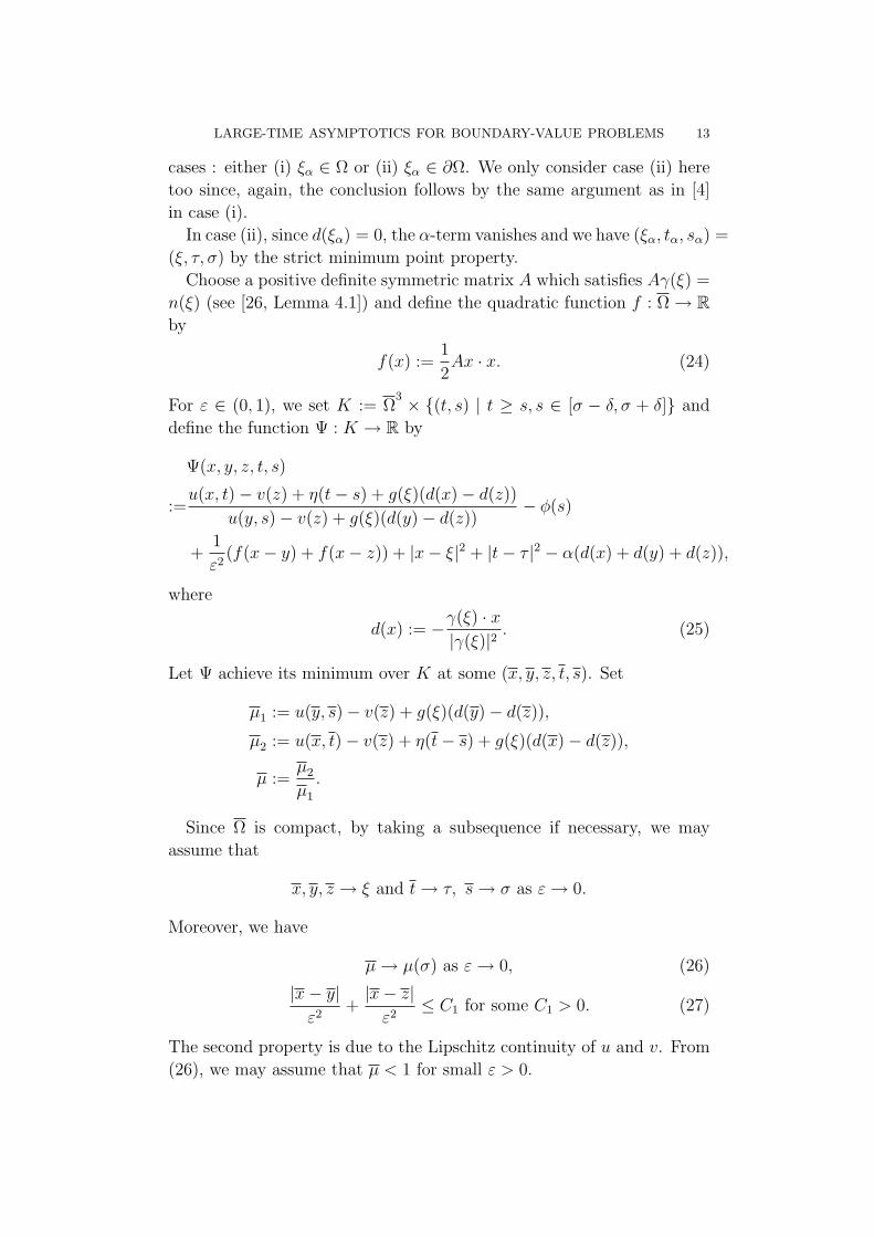
LARGE-TIME ASYMPTOTICS FOR BOUNDARY-VALUE PROBLEMS 13
cases : either (i) ξα ∈ Ω or (ii) ξα ∈ ∂Ω. We only consider case (ii) here
too since, again, the conclusion follows by the same argument as in [4]
in case (i).
In case (ii), since d(ξα) = 0, the α-term vanishes and we have (ξα, tα, sα) =
(ξ, τ, σ) by the strict minimum point property.
Choose a positive definite symmetric matrix A which satisfies Aγ(ξ) =
n(ξ) (see [26, Lemma 4.1]) and define the quadratic function f : Ω → Rby
f(x) :=1
2Ax · x. (24)
For ε ∈ (0, 1), we set K := Ω3 × (t, s) | t ≥ s, s ∈ [σ − δ, σ + δ] and
define the function Ψ : K → R by
Ψ(x, y, z, t, s)
:=u(x, t) − v(z) + η(t− s) + g(ξ)(d(x) − d(z))
u(y, s) − v(z) + g(ξ)(d(y) − d(z))− ϕ(s)
+1
ε2(f(x− y) + f(x− z)) + |x− ξ|2 + |t− τ |2 − α(d(x) + d(y) + d(z)),
where
d(x) := −γ(ξ) · x|γ(ξ)|2
. (25)
Let Ψ achieve its minimum over K at some (x, y, z, t, s). Set
µ1 := u(y, s) − v(z) + g(ξ)(d(y) − d(z)),
µ2 := u(x, t) − v(z) + η(t− s) + g(ξ)(d(x) − d(z)),
µ :=µ2
µ1
.
Since Ω is compact, by taking a subsequence if necessary, we may
assume that
x, y, z → ξ and t→ τ, s→ σ as ε→ 0.
Moreover, we have
µ→ µ(σ) as ε→ 0, (26)
|x− y|ε2
+|x− z|ε2
≤ C1 for some C1 > 0. (27)
The second property is due to the Lipschitz continuity of u and v. From
(26), we may assume that µ < 1 for small ε > 0.
14 G. BARLES AND H. MITAKE
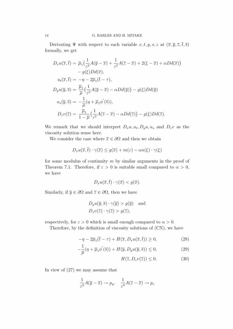
Derivating Ψ with respect to each variable x, t, y, s, z at (x, y, z, t, s)
formally, we get
Dxu(x, t) = µ1
( 1
ε2A(y − x) +
1
ε2A(z − x) + 2(ξ − x) + αDd(x)
)− g(ξ)Dd(x),
ut(x, t) = −η − 2µ1(t− τ),
Dyu(y, s) =µ1
µ
( 1
ε2A(y − x) − αDd(y)
)− g(ξ)Dd(y)
us(y, s) = − 1
µ(η + µ1ϕ
′(s)),
Dzv(z) =µ1
1 − µ
( 1
ε2A(z − x) − αDd(z)
)− g(ξ)Dd(z).
We remark that we should interpret Dxu, ut, Dyu, us and Dzv as the
viscosity solution sense here.
We consider the case where x ∈ ∂Ω and then we obtain
Dxu(x, t) · γ(x) ≤ g(x) +m(ε) − αn(ξ) · γ(ξ)
for some modulus of continuity m by similar arguments in the proof of
Theorem 7.1. Therefore, if ε > 0 is suitable small compared to α > 0,
we have
Dxu(x, t) · γ(x) < g(x).
Similarly, if y ∈ ∂Ω and z ∈ ∂Ω, then we have
Dyu(y, s) · γ(y) > g(y) and
Dzv(z) · γ(z) > g(z),
respectively, for ε > 0 which is small enough compared to α > 0.
Therefore, by the definition of viscosity solutions of (CN), we have
−η − 2µ1(t− τ) +H(x,Dxu(x, t)) ≥ 0, (28)
− 1
µ(η + µ1ϕ
′(s)) +H(y,Dyu(y, s)) ≤ 0, (29)
H(z,Dzv(z)) ≤ 0. (30)
In view of (27) we may assume that
1
ε2A(y − x) → py,
1
ε2A(z − x) → pz
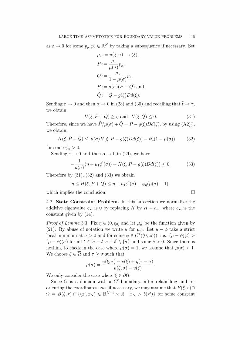
LARGE-TIME ASYMPTOTICS FOR BOUNDARY-VALUE PROBLEMS 15
as ε→ 0 for some py, pz ∈ RN by taking a subsequence if necessary. Set
µ1 := u(ξ, σ) − v(ξ),
P :=µ1
µ(σ)py,
Q :=µ1
1 − µ(σ)pz,
P := µ(σ)(P −Q) and
Q := Q− g(ξ)Dd(ξ).
Sending ε→ 0 and then α→ 0 in (28) and (30) and recalling that t→ τ ,
we obtain
H(ξ, P + Q) ≥ η and H(ξ, Q) ≤ 0. (31)
Therefore, since we have P /µ(σ) + Q = P − g(ξ)Dd(ξ), by using (A2)+0 ,
we obtain
H(ξ, P + Q) ≤ µ(σ)H(ξ, P − g(ξ)Dd(ξ)) − ψη(1 − µ(σ)) (32)
for some ψη > 0.
Sending ε→ 0 and then α → 0 in (29), we have
− 1
µ(σ)(η + µ1ϕ
′(σ)) +H(ξ, P − g(ξ)Dd(ξ)) ≤ 0. (33)
Therefore by (31), (32) and (33) we obtain
η ≤ H(ξ, P + Q) ≤ η + µ1ϕ′(σ) + ψη(µ(σ) − 1),
which implies the conclusion.
4.2. State Constraint Problem. In this subsection we normalize the
additive eigenvalue csc is 0 by replacing H by H − csc, where csc is the
constant given by (14).
Proof of Lemma 3.3. Fix η ∈ (0, η0] and let µ+η be the function given by
(21). By abuse of notation we write µ for µ+η . Let µ − ϕ take a strict
local minimum at σ > 0 and for some ϕ ∈ C1((0,∞)), i.e., (µ− ϕ)(t) >
(µ− ϕ)(σ) for all t ∈ [σ − δ, σ + δ] \ σ and some δ > 0. Since there is
nothing to check in the case where µ(σ) = 1, we assume that µ(σ) < 1.
We choose ξ ∈ Ω and τ ≥ σ such that
µ(σ) =u(ξ, τ) − v(ξ) + η(τ − σ)
u(ξ, σ) − v(ξ).
We only consider the case where ξ ∈ ∂Ω.
Since Ω is a domain with a C0-boundary, after relabelling and re-
orienting the coordinates axes if necessary, we may assume that B(ξ, r)∩Ω = B(ξ, r) ∩ (x′, xN) ∈ RN−1 × R | xN > b(x′) for some constant
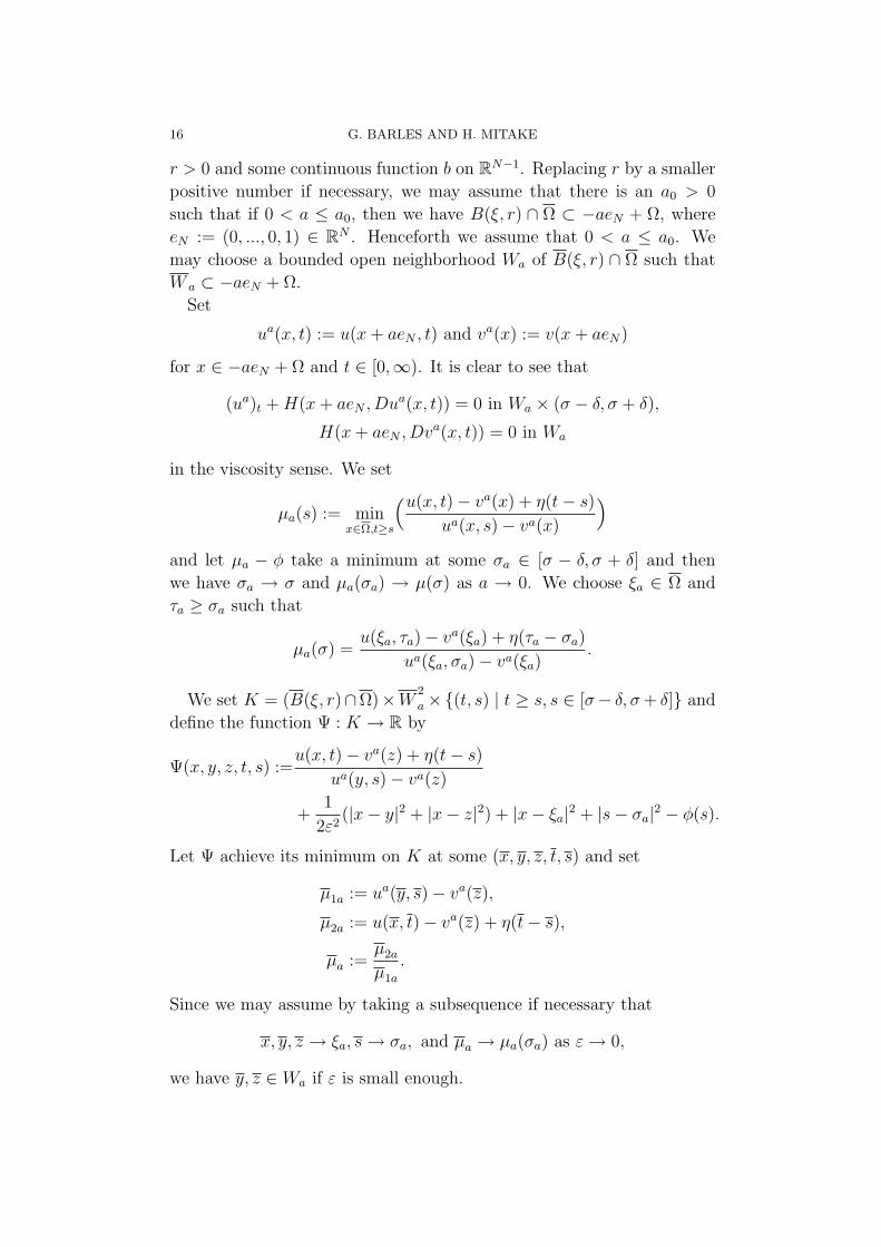
16 G. BARLES AND H. MITAKE
r > 0 and some continuous function b on RN−1. Replacing r by a smaller
positive number if necessary, we may assume that there is an a0 > 0
such that if 0 < a ≤ a0, then we have B(ξ, r) ∩ Ω ⊂ −aeN + Ω, where
eN := (0, ..., 0, 1) ∈ RN . Henceforth we assume that 0 < a ≤ a0. We
may choose a bounded open neighborhood Wa of B(ξ, r) ∩ Ω such that
W a ⊂ −aeN + Ω.
Set
ua(x, t) := u(x+ aeN , t) and va(x) := v(x+ aeN)
for x ∈ −aeN + Ω and t ∈ [0,∞). It is clear to see that
(ua)t +H(x+ aeN , Dua(x, t)) = 0 in Wa × (σ − δ, σ + δ),
H(x+ aeN , Dva(x, t)) = 0 in Wa
in the viscosity sense. We set
µa(s) := minx∈Ω,t≥s
(u(x, t) − va(x) + η(t− s)
ua(x, s) − va(x)
)and let µa − ϕ take a minimum at some σa ∈ [σ − δ, σ + δ] and then
we have σa → σ and µa(σa) → µ(σ) as a → 0. We choose ξa ∈ Ω and
τa ≥ σa such that
µa(σ) =u(ξa, τa) − va(ξa) + η(τa − σa)
ua(ξa, σa) − va(ξa).
We set K = (B(ξ, r)∩Ω)×W2
a ×(t, s) | t ≥ s, s ∈ [σ− δ, σ+ δ] and
define the function Ψ : K → R by
Ψ(x, y, z, t, s) :=u(x, t) − va(z) + η(t− s)
ua(y, s) − va(z)
+1
2ε2(|x− y|2 + |x− z|2) + |x− ξa|2 + |s− σa|2 − ϕ(s).
Let Ψ achieve its minimum on K at some (x, y, z, t, s) and set
µ1a := ua(y, s) − va(z),
µ2a := u(x, t) − va(z) + η(t− s),
µa :=µ2a
µ1a
.
Since we may assume by taking a subsequence if necessary that
x, y, z → ξa, s→ σa, and µa → µa(σa) as ε→ 0,
we have y, z ∈ Wa if ε is small enough.
LARGE-TIME ASYMPTOTICS FOR BOUNDARY-VALUE PROBLEMS 17
Therefore, by the definition of viscosity solutions we have
−η +H(x,Dxu(x, t)) ≥ 0, (34)
− 1
µa
(η + µ1a(ϕ
′(s) − 2(s− σa)) +H(y + aeN , Dyu
a(y, s)) ≤ 0, (35)
H(z + aeN , Dzva(z)) ≤ 0, (36)
where
Dxu(x, t) =µ1a
(y − x
ε2+z − x
ε2+ 2(ξa − x)
),
Dyua(y, s) =
µ1a
µa
· y − x
ε2,
Dzva(z) =
µ1a
1 − µa
· z − x
ε2.
In view of the Lipschitz continuity of ua on W a, we see that
y−xε2
ε,
z−xε2
ε
are bounded uniformly in ε > 0. Thus we may assume that
y − x
ε2→ pa
y,z − x
ε2→ pa
z ,
µ1a → µ1a := ua(ξa, σa) − va(ξa),
µa → µa(σa)
as ε→ 0 for some pay, p
az ∈ RN by taking a subsequence if necessary. Set
Pa :=µ1a
µa(σa)pa
y,
Qa :=µ1a
1 − µa(σa)pa
z and
Pa := µa(σa)(Pa −Qa).
Sending ε→ 0 in inequalities (34), (35) and (36) yields
−η +H(ξa, Pa +Qa) ≥ 0,
− 1
µa(σa)(η + µ1aϕ
′(σa)) +H(ξa + aeN , Pa) ≤ 0, (37)
H(ξa + aeN , Qa) ≤ 0.
Note that |Pa| + |Qa| ≤ R for some R > 0 which is independent of a.
There exists a modulus ωR such that
H(ξa + aeN , Pa +Qa) ≥ η − ωR(a). (38)
For small a > 0 we have
H(ξa + aeN , Pa +Qa) ≥η
2.
18 G. BARLES AND H. MITAKE
Since we have Pa/µa(σa) + Qa = Pa, by using (A2)+0 , we obtain
µa(σa)H(ξa + aeN , Pa) ≥ H(ξa + aeN , Pa +Qa) + ψη(1 − µa(σa)) (39)
for a constant ψη > 0.
By (38), (39) and (37) we get
η − ωR(a) ≤H(ξa + aeN , Pa +Qa)
≤µa(σa)H(ξa + aeN , Pa) − ψη(1 − µa(σa))
≤ η + µ1aϕ′(σa) − ψη(1 − µa(σa)).
We divide by µ1a > 0 and then we obtain
0 ≤ ϕ′(σa) +
ψη
µ1a
(µa(σa) − 1) +ωR(a)
µ1a
≤ ϕ′(σa) +
ψη
C(µa(σa) − 1) + ωR(a).
Sending a→ 0 yields
ϕ′(σ) +
ψη
C(µ(σ) − 1) ≥ 0,
which is the conclusion.
4.3. Dirichlet Problem. Let u be the solution of (CD) and csc be the
constant defined by (14).
We first treat the case where csc > 0. Set ucsc(x, t) = u(x, t) + csct
for (x, t) ∈ Ω × [0,∞) and gcsc(x, t) = g(x) + csct for (x, t) ∈ ∂Ω ×(0,∞). Since ucsc is bounded on Ω× [0,∞) by Proposition 2.1 (iii-a) and
gcsc(x, t) → ∞ uniformly for x ∈ ∂Ω as t → ∞, there exists a constant
t > 0 such that gcsc(x, t) > ucsc(x, t) for all (x, t) ∈ (t, ∞). As ucsc
satisfies (ucsc)t +H(x,Ducsc) = csc in Ω × (0,∞),
ucsc(x, t) = gcsc(x, t) on ∂Ω × (0,∞)
in the viscosity sense, we see easily that ucsc is a solution of(ucsc)t +H(x,Ducsc) ≤ csc in Ω × (t,∞),
(ucsc)t +H(x,Ducsc) ≥ csc on Ω × (t,∞).
Therefore the large-time asymptotic behavior of ucsc is same as the large-
time asymptotic behavior of solutions of (SC).
Next we consider the case where csc ≤ 0. Let v be a subsolution of
(D)0. Since u is bounded on Ω × [0,∞) by Proposition 2.1 (iii-b) and
v −M are still subsolutions of (D)0 for any M > 0, by subtracting a
positive constant to v if necessary, we may assume that u − v satisfies
(20).
LARGE-TIME ASYMPTOTICS FOR BOUNDARY-VALUE PROBLEMS 19
Let µ+η be the function defined by (21) for η ∈ (0, η0]. By abuse of
notation we write µ for µ+η . We prove that µ satisfies (22). We first
notice that, in view of the coercivity of H, we have
u(x, t) ≤ g(x) and (40)
v(x) ≤ g(x) for all (x, t) ∈ ∂Ω × (0,∞)
by Proposition 7.2.
Let ε > 0, ξ ∈ Ω, σ, τ ∈ (0,∞) and (x, t) ∈ Ω × [0,∞) be the same as
those in the proof of Lemma 3.3 in the case of (SC). We only consider
the case where µ(τ) < 1 and ξ ∈ ∂Ω. Since we have
0 ≤ µ(τ) =u(ξ, τ) − v(ξ) + η(τ − σ)
u(ξ, σ) − v(ξ)< 1
and u(ξ, σ) − v(ξ) > 0, we obtain
u(ξ, τ) − v(ξ) + η(τ − σ) < u(ξ, σ) − v(ξ) ≤ g(ξ) − v(ξ),
which implies u(ξ, τ) < g(ξ). Therefore we have u(x, t) − g(x) < 0 for
small ε > 0. The rest of the proof follows by the same method as in
subsection 4.2.
5. Convergence
In this section, we prove Theorem 1.3 by using Theorem 3.1.
Proof of Theorem 1.3. Let c be the associated additive eigenvalue. When
we consider (CD), let us set c := csc if csc > 0 and c := 0 if csc ≤ 0.
Since uc(·, t)t≥0 is compact in W 1,∞(Ω), there exists a sequence
uc(·, Tn)n∈N which converges uniformly on Ω as n → ∞. The max-
imum principle implies that we have
∥uc(·, Tn + ·) − uc(·, Tm + ·)∥L∞(Ω×(0,∞)) ≤ ∥uc(·, Tn) − uc(·, Tm)∥L∞(Ω)
for any n,m ∈ N. Therefore, uc(·, Tn + ·)n∈N is a Cauchy sequence
in BUC (Ω × [0,∞)) and it converges to a function denoted by u∞c ∈BUC (Ω × [0,∞)).
Fix any x ∈ Ω and s, t ∈ [0,∞) with t ≥ s. By Theorem 3.1 we have
uc(x, s+ Tn) − uc(x, t+ Tn) + η(s− t) ≤ δη(s+ Tn)
or
uc(x, t+ Tn) − uc(x, s+ Tn) − η(t− s) ≤ δη(s+ Tn)
for any n ∈ N and η > 0. Sending n → ∞ and then η → 0, we get, for
any t ≥ s
u∞c (x, s) ≤ u∞c (x, t).
20 G. BARLES AND H. MITAKE
or
u∞c (x, t) ≤ u∞c (x, s).
Therefore, we see that the functions x 7→ u∞c (x, t) are uniformly bounded
and equi-continuous which are also monotone in t. This implies that
u∞c (x, t) → w(x) uniformly on Ω as t → ∞ for some w ∈ W 1,∞(Ω).
Moreover, by a standard stability property of viscosity solutions, w is a
solution of either (E) or (D)0.
Since uc(·, Tn + ·) → u∞c uniformly in Ω × [0,∞) as n→ ∞, we have
−on(1) + u∞c (x, t) ≤ uc(x, Tn + t) ≤ u∞c (x, t) + on(1),
where on(1) → ∞ as n → ∞, uniformly in x and t. Taking the half-
relaxed semi-limits as t→ +∞, we get
−on(1) + v(x) ≤ liminf∗t→∞
[uc](x, t) ≤ limsup∗t→∞
[uc](x, t) ≤ v(x) + on(1).
Sending n→ ∞ yields
v(x) = liminf∗t→∞
[uc](x, t) = limsup∗t→∞
[uc](x, t)
for all x ∈ Ω.
Remark 1.
(i) The Lipschitz regularity assumption on u0 is convenient to avoid tech-
nicalities but it is not necessary. We can remove it as follows. We may
choose a sequence uk0k∈N ⊂ W 1,∞(Ω) ∩C(Ω) so that ∥uk
0 − u0∥L∞(Ω) ≤1/k for all n ∈ N. By the maximum principle, we have
∥u− uk∥L∞(Ω×(0,∞)) ≤ ∥uk0 − u0∥L∞(Ω) ≤ 1/k
and therefore
uk(x, t) − 1/k ≤ u(x, t) ≤ uk(x, t) + 1/k for all (x, t) ∈ Ω × [0,∞),
where u is the solution of (IB) and uk are the solutions of (IB) with
u0 = uk0. Therefore we have
uk∞(x) − 1/k ≤ liminf∗
t→∞u(x, t) ≤ limsup∗
t→∞u(x, t) ≤ uk
∞(x) + 1/k
for all x ∈ Ω, where uk∞(x) = limt→∞ uk(x, t). Thus, | liminf∗t→∞ u(x, t)−
limsup∗t→∞ u(x, t)| ≤ 2/k for all k ∈ N and x ∈ Ω, which implies that
liminf∗t→∞
u(x, t) = limsup∗t→∞
u(x, t)
for all x ∈ Ω. We note that, by the same argument, we can obtain the
asymptotic monotone property, Theorem 3.1, of solutions of (IB) without
the Lipschitz continuity of solutions.
LARGE-TIME ASYMPTOTICS FOR BOUNDARY-VALUE PROBLEMS 21
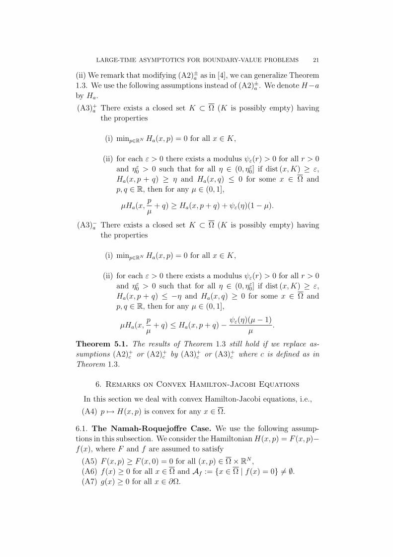
(ii) We remark that modifying (A2)±a as in [4], we can generalize Theorem
1.3. We use the following assumptions instead of (A2)±a . We denote H−aby Ha.
(A3)+a There exists a closed set K ⊂ Ω (K is possibly empty) having
the properties
(i) minp∈RN Ha(x, p) = 0 for all x ∈ K,
(ii) for each ε > 0 there exists a modulus ψε(r) > 0 for all r > 0
and ηε0 > 0 such that for all η ∈ (0, ηε
0] if dist (x,K) ≥ ε,
Ha(x, p + q) ≥ η and Ha(x, q) ≤ 0 for some x ∈ Ω and
p, q ∈ R, then for any µ ∈ (0, 1],
µHa(x,p
µ+ q) ≥ Ha(x, p+ q) + ψε(η)(1 − µ).
(A3)−a There exists a closed set K ⊂ Ω (K is possibly empty) having
the properties
(i) minp∈RN Ha(x, p) = 0 for all x ∈ K,
(ii) for each ε > 0 there exists a modulus ψε(r) > 0 for all r > 0
and ηε0 > 0 such that for all η ∈ (0, ηε
0] if dist (x,K) ≥ ε,
Ha(x, p + q) ≤ −η and Ha(x, q) ≥ 0 for some x ∈ Ω and
p, q ∈ R, then for any µ ∈ (0, 1],
µHa(x,p
µ+ q) ≤ Ha(x, p+ q) − ψε(η)(µ− 1)
µ.
Theorem 5.1. The results of Theorem 1.3 still hold if we replace as-
sumptions (A2)+c or (A2)+
c by (A3)+c or (A3)+
c where c is defined as in
Theorem 1.3.
6. Remarks on Convex Hamilton-Jacobi Equations
In this section we deal with convex Hamilton-Jacobi equations, i.e.,
(A4) p 7→ H(x, p) is convex for any x ∈ Ω.
6.1. The Namah-Roquejoffre Case. We use the following assump-
tions in this subsection. We consider the HamiltonianH(x, p) = F (x, p)−f(x), where F and f are assumed to satisfy
(A5) F (x, p) ≥ F (x, 0) = 0 for all (x, p) ∈ Ω × RN ,
(A6) f(x) ≥ 0 for all x ∈ Ω and Af := x ∈ Ω | f(x) = 0 = ∅.(A7) g(x) ≥ 0 for all x ∈ ∂Ω.
22 G. BARLES AND H. MITAKE
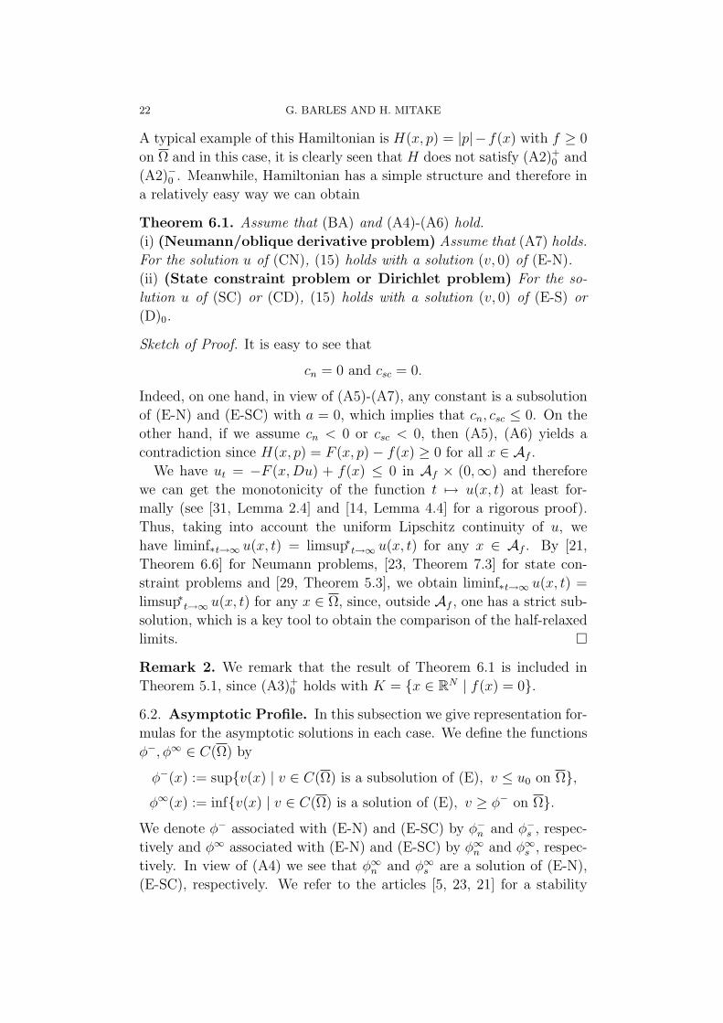
A typical example of this Hamiltonian is H(x, p) = |p|−f(x) with f ≥ 0
on Ω and in this case, it is clearly seen that H does not satisfy (A2)+0 and
(A2)−0 . Meanwhile, Hamiltonian has a simple structure and therefore in
a relatively easy way we can obtain
Theorem 6.1. Assume that (BA) and (A4)-(A6) hold.
(i) (Neumann/oblique derivative problem) Assume that (A7) holds.
For the solution u of (CN), (15) holds with a solution (v, 0) of (E-N).
(ii) (State constraint problem or Dirichlet problem) For the so-
lution u of (SC) or (CD), (15) holds with a solution (v, 0) of (E-S) or
(D)0.
Sketch of Proof. It is easy to see that
cn = 0 and csc = 0.
Indeed, on one hand, in view of (A5)-(A7), any constant is a subsolution
of (E-N) and (E-SC) with a = 0, which implies that cn, csc ≤ 0. On the
other hand, if we assume cn < 0 or csc < 0, then (A5), (A6) yields a
contradiction since H(x, p) = F (x, p) − f(x) ≥ 0 for all x ∈ Af .
We have ut = −F (x,Du) + f(x) ≤ 0 in Af × (0,∞) and therefore
we can get the monotonicity of the function t 7→ u(x, t) at least for-
mally (see [31, Lemma 2.4] and [14, Lemma 4.4] for a rigorous proof).
Thus, taking into account the uniform Lipschitz continuity of u, we
have liminf∗t→∞ u(x, t) = limsup∗t→∞ u(x, t) for any x ∈ Af . By [21,
Theorem 6.6] for Neumann problems, [23, Theorem 7.3] for state con-
straint problems and [29, Theorem 5.3], we obtain liminf∗t→∞ u(x, t) =
limsup∗t→∞ u(x, t) for any x ∈ Ω, since, outside Af , one has a strict sub-
solution, which is a key tool to obtain the comparison of the half-relaxed
limits.
Remark 2. We remark that the result of Theorem 6.1 is included in
Theorem 5.1, since (A3)+0 holds with K = x ∈ RN | f(x) = 0.
6.2. Asymptotic Profile. In this subsection we give representation for-
mulas for the asymptotic solutions in each case. We define the functions
ϕ−, ϕ∞ ∈ C(Ω) by
ϕ−(x) := supv(x) | v ∈ C(Ω) is a subsolution of (E), v ≤ u0 on Ω,
ϕ∞(x) := infv(x) | v ∈ C(Ω) is a solution of (E), v ≥ ϕ− on Ω.
We denote ϕ− associated with (E-N) and (E-SC) by ϕ−n and ϕ−
s , respec-
tively and ϕ∞ associated with (E-N) and (E-SC) by ϕ∞n and ϕ∞
s , respec-
tively. In view of (A4) we see that ϕ∞n and ϕ∞
s are a solution of (E-N),
(E-SC), respectively. We refer to the articles [5, 23, 21] for a stability
LARGE-TIME ASYMPTOTICS FOR BOUNDARY-VALUE PROBLEMS 23
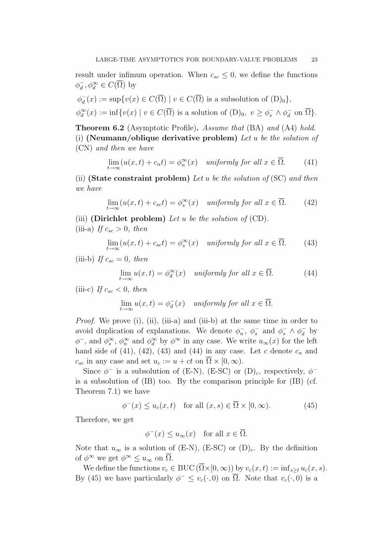
result under infimum operation. When csc ≤ 0, we define the functions
ϕ−d , ϕ
∞d ∈ C(Ω) by
ϕ−d (x) := supv(x) ∈ C(Ω) | v ∈ C(Ω) is a subsolution of (D)0,
ϕ∞d (x) := infv(x) | v ∈ C(Ω) is a solution of (D)0, v ≥ ϕ−
s ∧ ϕ−d on Ω.
Theorem 6.2 (Asymptotic Profile). Assume that (BA) and (A4) hold.
(i) (Neumann/oblique derivative problem) Let u be the solution of
(CN) and then we have
limt→∞
(u(x, t) + cnt) = ϕ∞n (x) uniformly for all x ∈ Ω. (41)
(ii) (State constraint problem) Let u be the solution of (SC) and then
we have
limt→∞
(u(x, t) + csct) = ϕ∞s (x) uniformly for all x ∈ Ω. (42)
(iii) (Dirichlet problem) Let u be the solution of (CD).
(iii-a) If csc > 0, then
limt→∞
(u(x, t) + csct) = ϕ∞s (x) uniformly for all x ∈ Ω. (43)
(iii-b) If csc = 0, then
limt→∞
u(x, t) = ϕ∞d (x) uniformly for all x ∈ Ω. (44)
(iii-c) If csc < 0, then
limt→∞
u(x, t) = ϕ−d (x) uniformly for all x ∈ Ω.
Proof. We prove (i), (ii), (iii-a) and (iii-b) at the same time in order to
avoid duplication of explanations. We denote ϕ−n , ϕ−
s and ϕ−s ∧ ϕ−
d by
ϕ−, and ϕ∞s , ϕ∞
n and ϕ∞d by ϕ∞ in any case. We write u∞(x) for the left
hand side of (41), (42), (43) and (44) in any case. Let c denote cn and
csc in any case and set uc := u+ ct on Ω × [0,∞).
Since ϕ− is a subsolution of (E-N), (E-SC) or (D)c, respectively, ϕ−
is a subsolution of (IB) too. By the comparison principle for (IB) (cf.
Theorem 7.1) we have
ϕ−(x) ≤ uc(x, t) for all (x, s) ∈ Ω × [0,∞). (45)
Therefore, we get
ϕ−(x) ≤ u∞(x) for all x ∈ Ω.
Note that u∞ is a solution of (E-N), (E-SC) or (D)c. By the definition
of ϕ∞ we get ϕ∞ ≤ u∞ on Ω.
We define the functions vc ∈ BUC (Ω×[0,∞)) by vc(x, t) := infs≥t uc(x, s).
By (45) we have particularly ϕ− ≤ vc(·, 0) on Ω. Note that vc(·, 0) is a
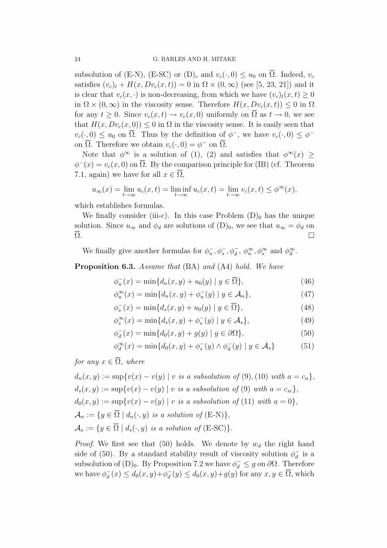
24 G. BARLES AND H. MITAKE
subsolution of (E-N), (E-SC) or (D)c and vc(·, 0) ≤ u0 on Ω. Indeed, vc
satisfies (vc)t +H(x,Dvc(x, t)) = 0 in Ω × (0,∞) (see [5, 23, 21]) and it
is clear that vc(x, ·) is non-decreasing, from which we have (vc)t(x, t) ≥ 0
in Ω × (0,∞) in the viscosity sense. Therefore H(x,Dvc(x, t)) ≤ 0 in Ω
for any t ≥ 0. Since vc(x, t) → vc(x, 0) uniformly on Ω as t → 0, we see
that H(x,Dvc(x, 0)) ≤ 0 in Ω in the viscosity sense. It is easily seen that
vc(·, 0) ≤ u0 on Ω. Thus by the definition of ϕ−, we have vc(·, 0) ≤ ϕ−
on Ω. Therefore we obtain vc(·, 0) = ϕ− on Ω.
Note that ϕ∞ is a solution of (1), (2) and satisfies that ϕ∞(x) ≥ϕ−(x) = vc(x, 0) on Ω. By the comparison principle for (IB) (cf. Theorem
7.1, again) we have for all x ∈ Ω,
u∞(x) = limt→∞
uc(x, t) = lim inft→∞
uc(x, t) = limt→∞
vc(x, t) ≤ ϕ∞(x),
which establishes formulas.
We finally consider (iii-c). In this case Problem (D)0 has the unique
solution. Since u∞ and ϕd are solutions of (D)0, we see that u∞ = ϕd on
Ω.
We finally give another formulas for ϕ−n , ϕ
−s , ϕ
−d , ϕ∞
n , ϕ∞s and ϕ∞
d .
Proposition 6.3. Assume that (BA) and (A4) hold. We have
ϕ−n (x) = mindn(x, y) + u0(y) | y ∈ Ω, (46)
ϕ∞n (x) = mindn(x, y) + ϕ−
n (y) | y ∈ An, (47)
ϕ−s (x) = minds(x, y) + u0(y) | y ∈ Ω, (48)
ϕ∞s (x) = minds(x, y) + ϕ−
s (y) | y ∈ As, (49)
ϕ−d (x) = mind0(x, y) + g(y) | y ∈ ∂Ω, (50)
ϕ∞d (x) = mind0(x, y) + ϕ−
s (y) ∧ ϕ−d (y) | y ∈ As (51)
for any x ∈ Ω, where
dn(x, y) := supv(x) − v(y) | v is a subsolution of (9), (10) with a = cn,ds(x, y) := supv(x) − v(y) | v is a subsolution of (9) with a = csc,d0(x, y) := supv(x) − v(y) | v is a subsolution of (11) with a = 0,
An := y ∈ Ω | dn(·, y) is a solution of (E-N),
As := y ∈ Ω | ds(·, y) is a solution of (E-SC).
Proof. We first see that (50) holds. We denote by wd the right hand
side of (50). By a standard stability result of viscosity solution ϕ−d is a
subsolution of (D)0. By Proposition 7.2 we have ϕ−d ≤ g on ∂Ω. Therefore
we have ϕ−d (x) ≤ d0(x, y)+ϕ
−d (y) ≤ d0(x, y)+g(y) for any x, y ∈ Ω, which
LARGE-TIME ASYMPTOTICS FOR BOUNDARY-VALUE PROBLEMS 25
implies that ϕ−d ≤ wd on Ω. It is easily seen that wd is a subsolution of
(D)0 and therefore wd ≤ ϕ−d on Ω.
We next prove (46) and (48). We denote ϕ−n , ϕ−
s and ϕ−s ∧ ϕ−
d by ϕ−
and denote by w− the right hand side of (46) and (48) in any case. Let
d denote dn or ds in any case. By the definition of ϕ− we see that ϕ−
is a subsolution of (E-N), (E-SC) or (D)0 and ϕ− ≤ u0 on Ω. By the
definition of d we have ϕ−(x) ≤ d(x, y) + ϕ−(y) ≤ d(x, y) + u0(y) for all
x, y ∈ Ω, which implies ϕ− ≤ w− on Ω. Note that w− is a subsolution
of (E-N), (E-SC) or (D)0 and w−(x) ≤ d(x, x) + u0(x) = u0(x) for all
x ∈ Ω. By the definition of ϕ− we obtain ϕ− = w− on Ω.
We finally prove (47), (49) and (51). We denote ϕ∞n , ϕ∞
s and ϕ∞d by
ϕ∞ and denote by w∞ the right hand side of (47), (49) and (51) in any
case. Let A denote An or As in any case.
It is easy to see that w∞(x) = ϕ−(x) for all x ∈ A. By [21, Theorem
6.6], [23, Theorem 7.3] and [29, Theorem 5.3] we get w∞ ≥ ϕ− on Ω. By
the definition of ϕ∞ we obtain w∞ ≥ ϕ∞ on Ω. Note that ϕ− ≤ ϕ∞ on
Ω. Then, we have
w∞(x) = ϕ−(x) ≤ ϕ∞(x) for all x ∈ A.
Therefore we get w∞ ≤ ϕ∞ on Ω by [21, Theorem 6.6], [23, Theorem 7.3]
and [29, Theorem 5.3].
6.3. On the compatibility condition (8). In this subsection we con-
sider (CD) under assumptions (A1), (A4) and (A2)+c or (A2)−c and we
remove the compatibility condition (8), where c := csc if csc > 0 and
c := 0 if csc ≤ 0. Let u be a solution of (CD). We notice that, if we do
not assume (8), then u may be discontinuous and therefore we interpret
solutions as discontinuous viscosity solutions introduced in [19].
We consider the following approximate problems of (CD)
(CD)1k
ut +H(x,Du) = 0 in Ω × (0,∞),
u(x, t) = g(x) on ∂Ω × (0,∞),
u(x, 0) = uk0(x) on Ω,
and
(CD)2k
ut +H(x,Du) = 0 in Ω × (0,∞),
u(x, t) = gk(x, t) on ∂Ω × (0,∞),
u(x, 0) = u0(x) on Ω,
26 G. BARLES AND H. MITAKE
where
uk0(x) := min
y∈Ωug
0(y) + k|x− y|2,
ug0(x) :=
u0(x) for x ∈ Ω,
u0(x) ∧ g(x) for x ∈ ∂Ω,
gk(x, t) := maxg(x), u0(x) − kt
for all x ∈ Ω, g ≥ 0 and k ∈ N. Note that
uk0(x) ≤ g(x) and u0(x) ≤ gk(x, t)
for all (x, t) ∈ ∂Ω × [0,∞) and k ∈ N.
Let u1k and u2
k be the solution of (CD)1k and (CD)2
k, respectively. By
Theorem 6.2 we have for any k ∈ Nif csc > 0, u1
k(·, t) + csct→ minds(·, y) + ϕ−k (y) | y ∈ As
if csc = 0, u1k(·, t) → minds(·, y) + ϕ−
k (y) ∧ ϕ−d (y) | y ∈ As,
if csc < 0, u1k(·, t) → ϕ−
d
uniformly on Ω as t→ ∞, where
ϕ−k (x) := minds(x, y) + uk
0(y) | y ∈ Ω for all x ∈ Ω.
By [30, Theorem 6.1] we have for any k ∈ Nif csc ≥ 0, u2
k(·, t) + csct→ minds(·, y) + ϕ−s (y) ∧ ϕ−
gk(y) | y ∈ As
if csc < 0, u2k(·, t) → ϕ−
d
uniformly on Ω as t→ ∞, where
ϕ−gk
(x) := infds(x, y) + gk(y) | y ∈ ∂Ω for all x ∈ Ω,
gk(x) := infgk(x, s) + cscs | s ≥ 0 for all x ∈ ∂Ω.
Proposition 6.4. We have ϕ−k → ϕ−
s uniformly on Ω as k → ∞.
Proof. It is easy to see that ϕ−k (x) is nondecreasing as k → ∞ for any
x ∈ Ω. We prove that ϕ−k (x) converges to ϕ−
s (x) ∧ ϕ−d (x) as k → ∞ for
any x ∈ Ω. Fix x ∈ Ω. First, we can easily see that lim supk→∞ ϕ−k (x) ≤
ϕ−s (x) ∧ ϕ−
d (x), since ϕ−k ≤ uk
0 ≤ ug0 on Ω.
Choose yk, zk ∈ Ω such that
ϕ−k (x) = ds(x, yk) + uk
0(yk) and
uk0(yk) = ug
0(zk) + k|yk − zk|2.
LARGE-TIME ASYMPTOTICS FOR BOUNDARY-VALUE PROBLEMS 27
Since Ω is compact, we may assume that yk, zk → y0 ∈ Ω as k → ∞ if
taking a subsequence if necessary. We have
lim infk→∞
ϕ−k (x) = lim inf
k→∞
(ds(x, yk) + uk
0(yk))
≥ lim infk→∞
(ds(x, yk) + ug
0(zk))
≥ ds(x, y0) + ug0(y0)
≥ ϕ−s (x) ∧ ϕ−
d (x).
Therefore we obtain lim supk→∞ ϕ−k (x) = lim infk→∞ ϕ−
k (x) = ϕ−s (x) ∧
ϕ−d (x). Since ϕ−
s ∧ϕ−d ∈ C(Ω), in view of Dini’s theorem, we see that the
convergence is uniform for all x ∈ Ω.
Proposition 6.5. We have ϕ−gk
→ ϕ−d uniformly on Ω as k → ∞.
Proof. We only need to consider csc ≥ 0 and prove that gk→ g uniformly
on ∂Ω as k → ∞. Fix x ∈ ∂Ω. Since gk(x, s) ≥ g(x) for all x ∈ ∂Ω and
s ≥ 0, we have gk(x) = infs≥0gk(x, s) + cscs ≥ g(x). Thus we have
lim infk→∞ gk(x) ≥ g(x) for all x ∈ ∂Ω.
Fix any s ∈ (0,∞). Then there exists k0 ∈ N such that for all k ≥ k0,
gk(x, s) = g(x). We get gk(x) ≤ gk(x, s) + cscs = gk(x) + cscs. Therefore
we have lim supk→∞ gk(x) ≤ g(x) + cscs. Sending s → 0, we obtain
lim supk→∞ gk(x) ≤ g(x). Noting that g ∈ C(∂Ω) and g
kis nonincreasing
as k → ∞, in view of Dini’s theorem we get a conclusion. By the comparison principle for (IB) we have
u1k ≤ u ≤ u2
k on Ω × [0,∞) for all k ∈ N.
By Propositions 6.4, 6.5 we obtain
limsup∗t→∞
u = liminf∗t→∞
u = limk→∞
u1k = lim
k→∞u2
k on Ω.
7. Appendix : Existence, Uniqueness and Regularity
Results for (IB)
All the results presented in this appendix may appear at first glance
as being well-known and covered by the standard results of the theory of
viscosity solutions (see for instance [25, 21, 1, 7]). But some of them are
not completely standard because we are dealing with an oblique vector
field γ which is only continuous (and not Lipschitz continuous as in the
standard cases) and with a domain Ω which is not very regular. Of course,
we can extend the classical results to this more general framework because
the solutions of (IB) are expected to be in W 1,∞ since the Hamiltonian is
coercive. But we have also to prove directly the existence of such W 1,∞
-solutions, by using only comparison results which hold for W 1,∞ sub
28 G. BARLES AND H. MITAKE
and supersolutions, which is a little bit unusual in the theory of viscosity
solutions.
Also, we remark that the calculations in the proof of comparison prin-
ciples are used in the proofs of a key ingredient, Lemma 3.3, in order to
prove the asymptotic monotone property, Theorem 1.3. Therefore, re-
minding the proofs of the comparison principles helps us to understand
them.
Before providing these results and their proofs, we recall, for the
reader’s convenience, the definition of viscosity solutions for (IB), and
in particular of boundary conditions in the viscosity sense (see [8] for
instance).
Definition 1. An upper-semicontinuous function u (resp., a lower semi-
continuous function u) is a subsolution (resp., supersolution) of (IB) if
the following conditions hold:
(i) u is a (viscosity) subsolution (resp., (viscosity) supersolution) of (1),
(ii) u(x, 0) ≤ u0(x) (resp., u(x, 0) ≥ u0(x)) for all x ∈ Ω, and
(iii) for any ϕ ∈ C1(Ω× [0,∞)) and any (x0, t0) ∈ ∂Ω× (0,∞) such that
u− ϕ takes a local maximum (resp., minimum) at (x0, t0),
minϕt(x0, t0) +H(x0, Dϕ(x0, t0)), B(x0, u(x0, t0), Dϕ(x0, t0)) ≤ 0
(resp.,
maxϕt(x0, t0) +H(x0, Dϕ(x0, t0)), B(x0, u(x0, t0), Dϕ(x0, t0)) ≥ 0).
We call u a solution of (IB) if it is a subsolution and a supersolution of
(IB).
7.1. Comparison Results for (IB).
Theorem 7.1. Assume that (BA) holds.
(i) (Neumann/oblique derivative problem) Let u ∈ C(Ω × [0,∞)),
v ∈ LSC (Ω × [0,∞)) be a subsolution and a supersolution of (CN),
respectively. If u(·, 0) ≤ v(·, 0) on Ω, then u ≤ v on Ω × [0,∞).
(ii) (State constraint or Dirichlet problem) Let u ∈ C(Ω× [0,∞)),
v ∈ LSC (Ω × [0,∞)) be a subsolution and a supersolution of (SC) or
(CD), respectively. If u(·, 0) ≤ v(·, 0) on Ω, then u ≤ v on Ω × [0,∞).
Remark 3. It is worth mentioning that it is well known that there exists
a discontinuous solution of (SC) and (CD), which implies that in the
comparison principle for (SC) and (CD), we can not replace requirements
of continuity of u by that of semicontinuity.
Proof of Theorem 7.1 (i). We argue by contradiction assuming that there
would exist T > 0 such that maxQT(u − v)(x, t) > 0, where QT :=
Ω × (0, T ).
LARGE-TIME ASYMPTOTICS FOR BOUNDARY-VALUE PROBLEMS 29
Let uδ denote the function
uδ(x, t) := maxs∈[0,T+2]
u(x, s) − (1/δ)(t− s)2 ,
for any δ > 0. This sup-convolution procedure is standard in the theory
of viscosity solutions (although, here, it acts only on the time-variable)
and it is known that, for δ small enough, uδ is a subsolution of (CN)
in Ω × (aδ, T + 1), where aδ := (2δmaxQT+2|u(x, t)|)1/2 (see [1, 8] for
instance).
Moreover, it is easy to check that |uδt | ≤ Cδ in Ω × (aδ, T + 1) and
therefore by the coercivity of H and the C1-regularity of ∂Ω we have, for
all x, y ∈ Ω, t, s ∈ [aδ, T + 1]
|uδ(x, t) − uδ(y, s)| ≤ Cδ(|x− y| + |t− s|) (52)
for some Cδ > 0. Finally, as δ → 0, maxQT(uδ − v)(x, t) → maxQT
(u −v)(x, t) > 0.
Therefore it is enough to consider maxQT(uδ − v)(x, t) for δ > 0 small
enough, and we follow the classical proof by introducing
maxQT
(uδ − v)(x, t) − ηt ,
for 0 < η ≪ 1. This maximum is achieved at (ξ, τ) ∈ Ω × [0, T ], namely
(uδ − v)(ξ, τ)− ηt = maxQT(uδ − v)(x, t)− ηt. Clearly τ depends on η
but we can assume that it remains bounded away from 0, otherwise we
easily get a contradiction.
We only consider the case where ξ ∈ ∂Ω. We define the function
Ψ : Ω2 × [0, T ] → R by
Ψ(x, y, t) :=uδ(x, t) − v(y, t) − ηt− 1
ε2f(x− y)
+ g(ξ)(d(x) − d(y)) + α(d(x) + d(y)) − |x− ξ|2 − (t− τ)2,
where f and d are given by (24) and (25). Let Ψ achieve its maximum
at (x, y, t) ∈ Ω2 × [0, T ]. By a standard arguments, we have
x, y → ξ and t→ τ as ε→ 0 (53)
by taking a subsequence if necessary and, because of the Lipschitz con-
tinuity (52) of uδ, we have
|x− y|ε2
≤ Cδ (54)
30 G. BARLES AND H. MITAKE
Derivating (formally) Ψ with respect to each variable x, y at (x, y, t),
we have
Dxuδ(x, t) =
1
ε2A(x− y) + 2(x− ξ) − αDd(x) − g(ξ)Dd(x),
Dyv(y, t) =1
ε2A(x− y) + αDd(y) − g(ξ)Dd(y).
We remark that we should interpret Dxuδ and Dyv in the viscosity solu-
tion sense here. We also point out that the viscosity inequalities we are
going to write down below, hold up to time T , in the spirit of [1], Lemma
2.8, p. 41.
Since Ω is a domain with a C1-boundary, we first observe that for any
x ∈ ∂Ω and y ∈ Ω
(x− y) · n(x) ≥ o(|x− y|),where o : [0,∞) → R is a continuous function such that |o(r)|/r → 0 as
r → 0.
Moreover, we have
A(x− y) · γ(x)≥ (x− y) · Aγ(ξ) − |y − x|mγ(|x− ξ|)= (x− y) · n(ξ) − |y − x|mγ(|x− ξ|)≥ (x− y) · n(x) − |y − x|
(mγ(|x− ξ|) +mn(|x− ξ|)
)≥ o(|x− y|) − |y − x|
(mγ(|x− y|) +mn(|x− ξ|)
),
where mγ and mn are modulus of continuity of γ, n on Ω, respectively.
Setting md := |o(r)|/r, by (54), we obtain
1
ε2A(x− y) · γ(x) ≥ −Cδ
(md(Cδε
2) +mγ(Cδε2) +mn(|x− ξ|)
). (55)
Moreover, we have
αDd(x) · γ(x) ≤ −α+ αmγ(|x− ξ|)
and
g(ξ)Dd(x) · γ(x) ≤ −g(x) +mg(|x− ξ|),
where mg is a modulus of continuity of g on ∂Ω. Therefore we have
Dxu(x, t) · γ(x) ≥ g(x) −m(ε) + α,
for a modulus m. Therefore, if ε > 0 is suitable small compared to α > 0,
we have
Dxu(x, t) · γ(x) > g(x).
Similarly, if y ∈ ∂Ω, then we have
Dyu(y, t) · γ(y) < g(y)
LARGE-TIME ASYMPTOTICS FOR BOUNDARY-VALUE PROBLEMS 31
for ε > 0 which is suitable small compared to α > 0.
Therefore, by the definition of viscosity solutions of (CN), using the
arguments of the User’s guide to viscosity solutions [8], there exists
a1, a2 ∈ R such that
a1 +H(x,1
ε2A(x− y) + 2(x− ξ) − αDd(x) − g(ξ)Dd(x)) ≤ 0,
a2 +H(y,1
ε2A(x− y) + αDd(x) − g(ξ)Dd(y)) ≥ 0
with a1 − a2 = η + 2(t− τ). By (54) we may assume that
1
ε2A(x− y) → p
as ε→ 0 for some p ∈ RN by taking a subsequence if necessary. Sending
ε→ 0 and then α→ 0 in the above inequalities, we have a contradiction
since a − b → η > 0 while the H-terms converge to the same limit.
Therefore τ cannot be assumed to remain bounded away from 0 and the
conclusion follows. Proof of Theorem 7.1 (ii). We only prove the comparison principle for
(CD), since we can regard (SC) as a problem of (CD) with the extreme
form “g(x) ≡ +∞”.
To justify this choice, we first prove the
Proposition 7.2. (Classical Dirichlet Boundary Conditions) As-
sume that (BA) holds. If u ∈ USC (Ω× [0,∞)) is a subsolution of (CD),
then u(x, t) ≤ g(x) for all (x, t) ∈ ∂Ω × (0,∞).
In the same way we can prove that, if u ∈ USC (Ω) is a subsolution of
(D)a for any a ≥ csc, then u(x) ≤ g(x) for all x ∈ ∂Ω.
Proof. Fix (x0, t0) ∈ ∂Ω×(0,∞). Fix r ∈ (0, t0) and set K :=(B(x0, r)∩
Ω)× [t0 − r, t0 + r]. Choose a sequence xkk∈N ⊂ RN \ Ω such that
|x0 − xk| = 1/k2. We define the function ϕ : K → R by
ϕ(x, t) = u(x, t) − k|x− xk| − αk(t− t0)2,
where αkk∈N ⊂ (0,∞) is a divergent sequence which will be fixed later.
Let (ξk, τk) ∈ K be a maximum point of ϕ on K. Noting that ϕ(ξk, τk) ≥ϕ(x0, t0), we have
k|ξk − xk| + αk(τk − t0)2 ≤ u(ξk, τk) − u(x0, t0) + k|x0 − xk| ≤ C, (56)
where C > 0 is a constant independent of k. From the above, we see
that ξk → x0, τk → t0 as k → ∞.
By the viscosity property of u, we have
qk +H(ξk, pk) ≤ 0 or u(ξk, τk) ≤ g(ξk),
32 G. BARLES AND H. MITAKE
if k ∈ N is sufficiently large, where pk = k(ξk − xk)/|ξk − xk| and qk =
2αk(τk − t0). Set f(k) := minx∈B(x0,r)∩ΩH(x, pk). Noting that |pk| = k,
by the coercivity of H, f(k) → ∞ as k → ∞. Choose αkk∈N ⊂ (0,∞)
such that
αk → ∞ as k → ∞ and 2√Cαk + 1 ≤ f(k) for sufficinetly large k ∈ N.
Since we have αk|τk − t0| ≤√Cαk for all k ∈ N by (56),
qk +H(xk, pk) ≥ −2αk|τk − t0| + f(k) ≥ −2√Cαk + f(k) ≥ 1 > 0
for sufficiently large k ∈ N, we must have u(ξk, τk) ≤ g(ξk). Sending
k → ∞, we obtain u(x0, t0) ≤ g(x0). Now we return to the proof of the comparison result for (CD). We argue
by contradiction, exactly in the same way as for (CN), introducing QT
and the function uδ which is a subsolution of (CD) in Ω× (aδ, T +1). We
still denote by (ξ, τ) ∈ Ω× [0, T ], a maximum point of (uδ − v)(x, t)− ηt,
namely
(uδ − v)(ξ, τ) − ητ = maxQT
(uδ − v)(x, t) − ηt .
Again we may assume that τ remains bounded away from 0, otherwise
the result would follow.
We only consider the case where ξ ∈ ∂Ω. Since Ω is a domain with
a C0-boundary, there exist r > 0, b ∈ C(RN−1,R) such that, after rela-
belling and re-orienting the coordinates axes if necessary, we may assume
B(ξ, r) ∩ Ω = B(ξ, r) ∩ (x′, xN) | xN > b(x′). There exists a0 > 0 such
that for any a ∈ (0, a0), there exists a bounded open neighborhood Wa
of B(ξ, r) ∩ Ω such that Wa ⊂ −aeN + Ω := −aeN + x | x ∈ Ω, where
eN := (0, . . . , 0, 1) ∈ RN .
Since (uδ − g)(ξ, τ) ≤ 0 in view of Proposition 7.2 and uδ(ξ, τ) −v(ξ, τ) > 0, we have v(ξ, τ) − g(ξ) < 0.
For any a ∈ (0, a0) and (x, t) ∈ W a × [0, T ], set uδa(x, t) := uδ(x +
aeN , t). Then, it is easily seen that uδa satisfies
(uδa)t(x, t) +H(x+ aeN , Du
δa(x, t)) ≤ 0 in Wa × (aδ, T + 1)
in the viscosity sense.
Let ε > 0 and define the function Ψ : W a × (B(ξ, r)∩Ω)× [0, T ] → Rby
Ψ(x, y, t, s) :=uδa(x, t) − v(y, t) − ηt
− 1
2ε2|x− y|2 − |y − ξ|2 − (t− τ)2.
Set V := W a×(B(ξ, r)∩Ω)× [0, T ] and let (x, y, t) ∈ V be a maximum
point of Ψ on V . By the compactness of V we may assume that x, y → xa
LARGE-TIME ASYMPTOTICS FOR BOUNDARY-VALUE PROBLEMS 33
and t → ta as ε → 0 by taking a subsequence if necessary. Taking the
limit as ε→ 0 in the inequality Ψ(x, y, t) ≥ Ψ(ξ, ξ, τ) yields
|xa − ξ|2 + |ta − τ |2 ≤ (uδa − v)(xa, ta) − ηta − (uδ
a − v)(ξ, τ) − ητ≤ (uδ − v)(xa, ta) − ηta − (uδ − v)(ξ, τ) − ητ
+ 2mu(a)
≤ 2mu(a),
where mu be a modulus of continuity of uδ on QT . We notice that we
use the continuity of u here.
Fix a small a ∈ (0, a0) so that v(xa, ta) − g(xa) < 0 and moreover we
may assume that v(y, t) − g(y) < 0 for y ∈ ∂Ω if ε is sufficiently small.
By the viscosity property of uδa and v and using classical arguments,
there exist b1, b2 ∈ R such that
b1 +H(x+ aeN ,x− y
ε2) ≤ 0, (57)
b2 +H(y,x− y
ε2− 2(y − ξ)) ≥ 0 (58)
with d1 − d2 = η + 2(t− τ). In view of the Lipschitz continuity of uδa on
W a× [0, T ], we have (x−y)/ε2 is bounded uniformly ε > 0 and therefore,
by sending ε→ 0 we may assume (x−y)/ε2 → pδ,a ∈ B(0, Cδ,a) for some
Cδ,a > 0. Noting that H is uniformly continuous on Ω × B(0, Cδ,a + 1),
we see that there exists a modulus mδ such that
H(x+aeN , p) ≥ H(x, p)−mδ(a) for any (x, p) ∈ Ω×B(0, Cδ+1). (59)
Combining (57) and (58) with (59), if a > 0 is small enough, we get
mδ(a) ≥ η + 2(t− τ) +H(x,x− y
ε2) −H(y,
x− y
ε2− 2(y − ξ)).
After taking the limit as ε → 0, send a → 0 and then we get η ≤ 0,
which is a contradiction. We have thus completed the proof.
7.2. Existence of Solutions of (IB).
Proof of Theorem 1.1. We present the proof of the existence of Lipschitz
continuous solutions of (IB).
Following similar arguments as in the proof of Theorem 1.2, it is easy
to prove that, for C > 0 large enough −Ct + u0(x) and Ct + u0(x) are,
respectively, viscosity subsolution and a supersolution of (CN) or (SC)
or (CD) with, of course, different constant C in each case.
By Perron’s method (see [19]) and Theorem 7.1 we obtain continuous
solutions of (IB) for (CN), (SC) and (CD) that we denote by u1, u2 and
34 G. BARLES AND H. MITAKE
u3, respectively. As a consequence of Perron’s method, we have
−Ct+ u0(x) ≤ ui(x, t) ≤ Ct+ u0(x) on Ω × [0,∞) ,
for i = 1, 2, 3.
To conclude, we use a standard argument : comparing the solutions
ui(x, t) and ui(x, t+ h) for some h > 0 and using the above property on
the ui, we have
∥ui(·, · + h) − ui(·, ·)∥∞ ≤ ∥ui(·, h) − ui(·, 0)∥∞ ≤ Ch .
As a consequence we have ∥(ui)t∥∞ ≤ C and, by using the equation
together with (A1), we obtain that Du is also bounded. This completes
the proof.
We finally remark that we can deduce the uniform continuity of so-
lutions of (IB) under the assumption u0 ∈ C(Ω). We may choose a
sequence uk0k∈N ⊂ W 1,∞(Ω) ∩ C(Ω) so that ∥uk
0 − u0∥L∞(Ω) ≤ 1/k for
all n ∈ N. Let uk be a solution of (IB) with u0 = uk0 and by the above
argument we see uk ∈ UC (Ω × [0,∞)) for all k ∈ N. The maximum
principle for (IB) implies that uk uniformly converges to u on Ω× [0,∞).
Thus we obtain u ∈ UC (Ω × [0,∞)).
Acknowledgements. Owing to a recent joint work [2] with Hitoshi
Ishii, the authors could refine the proof of Lemma 3.3 in the case of
Neumann problem on an early version of this paper. Moreover he gave
the second author helpful suggestions on Sections 6.3 and Proposition
7.2. The authors are grateful to him. This work was partially done
while the second author visited the Laboratoire de Mathematiques et
Physique Theorique, Universite de Tours and Mathematics Department,
University of California, Berkeley. He is grateful for their hospitality.
References
1. Barles, G. (1994). Solutions de viscosite des equations de Hamilton-Jacobi.Mathematiques & Applications (Berlin), 17, Springer-Verlag, Paris.
2. Barles, G., Ishii, H., Mitake, H., in preparation.3. Barles, G., Roquejoffre, J.-M. (2006). Ergodic type problems and large time be-
haviour of unbounded solutions of Hamilton-Jacobi equations. Comm. Partial Dif-ferential Equations 31, no. 7-9, 1209–1225.
4. Barles, G., Souganidis, P. E. (2000). On the large time behavior of solutions ofHamilton-Jacobi equations. SIAM J. Math. Anal. 31, no. 4, 925–939.
5. Barron, E. N., Jensen, R. (1990). Semicontinuous viscosity solutions for Hamilton-Jacobi equations with convex Hamiltonians. Comm. Partial Differential Equations15, no. 12, 1713–1742.
LARGE-TIME ASYMPTOTICS FOR BOUNDARY-VALUE PROBLEMS 35
6. Bernard, P., Roquejoffre, J.-M. (2004). Convergence to time-periodic solutions intime-periodic Hamilton-Jacobi equations on the circle. Comm. Partial DifferentialEquations 29, no. 3-4, 457–469.
7. Capuzzo-Dolcetta, I., Lions, P.-L. (1990). Hamilton-Jacobi equations with stateconstraints. Trans. Amer. Math. Soc. 318, no. 2, 643–683.
8. Crandall, M. G., Ishii, H., Lions, P.-L. (1992). User’s guide to viscosity solutionsof second order partial differential equations. Bull. Amer. Math. Soc. (N.S.) 27,no. 1, 1–67.
9. Davini, A., Siconolfi, A. (2006). A generalized dynamical approach to the largetime behavior of solutions of Hamilton-Jacobi equations. SIAM J. Math. Anal. 38,no. 2, 478–502.
10. Fathi, A. (1998). Sur la convergence du semi-groupe de Lax-Oleinik. C. R. Acad.Sci. Paris Ser. I Math. 327, no. 3, 267–270.
11. Fathi, A., Siconolfi, A. (2005). PDE aspects of Aubry-Mather theory for quasi-convex Hamiltonians. Calc. Var. Partial Differential Equations 22, no. 2, 185–228.
12. Fujita, Y., Loreti, P. (2009). Long-time behavior of solutions to Hamilton-Jacobiequations with quadratic gradient term. NoDEA Nonlinear Differential EquationsAppl. 16, no. 6, 771–791.
13. Fujita, Y., Uchiyama, K. (2007). Asymptotic solutions with slow convergence rateof Hamilton-Jacobi equations in Euclidean n space. Differential Integral Equations20, no. 10, 1185–1200.
14. Giga, Y. , Liu, Q., Mitake, H. (submitted). Singular Neumann problems andlarge-time behavior of solutions of non-coercive Hamitonian-Jacobi equations.
15. Giga, Y., Liu, Q., Mitake, H. (preprint). Large-time behavior of one-dimensionalDirichlet problems of Hamilton-Jacobi equations with non-coercive Hamiltonians.
16. Ichihara, N., Ishii, H. (2008). Asymptotic solutions of Hamilton-Jacobi equationswith semi-periodic Hamiltonians. Comm. Partial Differential Equations 33, no.4-6, 784–807.
17. Ichihara, N., Ishii, H. (2008). The large-time behavior of solutions of Hamilton-Jacobi equations on the real line. Methods Appl. Anal. 15, no. 2, 223–242.
18. Ichihara, N., Ishii, H. (2009). Long-time behavior of solutions of Hamilton-Jacobiequations with convex and coercive Hamiltonians. Arch. Ration. Mech. Anal. 194,no. 2, 383–419.
19. Ishii, H. (1987). Perron’s method for Hamilton-Jacobi equations. Duke Math. J.55, no. 2, 369–384.
20. Ishii, H. (2008). Asymptotic solutions for large time of Hamilton-Jacobi equationsin Euclidean n space. Ann. Inst. H. Poincare Anal. Non Lineaire, 25 (2008), no2, 231–266.
21. Ishii, H. (submitted). Weak KAM aspects of convex Hamilton-Jacobi equationswith Neumann type boundary conditions.
22. Ishii, H., (to appear). Long-time asymptotic solutions of convex Hamilton-Jacobiequations with Neumann type bouundary conditions. Calc. Var. Partial DifferentialEquations.
23. Ishii, H., Mitake, H. (2007). Representation formulas for solutions of Hamilton-Jacobi equations with convex Hamiltonians. Indiana Univ. Math. J., 56, no. 5,2159–2184.
36 G. BARLES AND H. MITAKE
24. Kruzkov, S. N. (1967). Generalized solutions of nonlinear equations of the firstorder with several independent variables. II, (Russian). Mat. Sb. (N.S.) 72 (114)108–134.
25. Lions, P.-L. (1985). Neumann type boundary conditions for Hamilton-Jacobiequations. Duke Math. J. 52, no. 4, 793–820.
26. Lions, P.-L., Sznitman, A.-S. (1984). Stochastic differential equations with reflect-ing boundary conditions. Comm. Pure Appl. Math. 37, no. 4, 511–537.
27. Lions, P.-L., Papanicolaou, G., Varadhan, S. R. S., (preprint). Homogenizationof Hamilton-Jacobi equations.
28. Mitake, H. (2008). Asymptotic solutions of Hamilton-Jacobi equations with stateconstraints. Appl. Math. Optim. 58, no. 3, 393–410.
29. Mitake, H. (2008). The large-time behavior of solutions of the Cauchy-Dirichletproblem for Hamilton-Jacobi equations. NoDEA Nonlinear Differential EquationsApp. 15, no. 3, 347–362.
30. Mitake, H. (2009). Large time behavior of solutions of Hamilton-Jacobi equationswith periodic boundary data. Nonlinear Anal. 71, no. 11, 5392–5405.
31. Namah G., Roquejoffre, J.-M. (1999). Remarks on the long time behaviour of thesolutions of Hamilton-Jacobi equations. Comm. Partial Differential Equations 24,no. 5-6, 883–893.
32. Roquejoffre, J.-M. (2001). Convergence to steady states or periodic solutions ina class of Hamilton-Jacobi equations. J. Math. Pures Appl. (9) 80, no. 1, 85–104.
(G. Barles) Laboratoire de Mathematiques et Physique Theorique (UMR
CNRS 6083), Federation Denis Poisson, Universite de Tours, Place de
Grandmont, 37200 Tours, FRANCE
E-mail address: [email protected]: http://www.lmpt.univ-tours.fr/~barles
(H. Mitake) Department of Applied Mathematics, Graduate School of
Engineering Hiroshima University Higashi-Hiroshima 739-8527, Japan
E-mail address: [email protected]