A Patient-Specific Poroelastic Model of a Brain with a ... · A Patient-Specific Poroelastic Model...

A Patient-Specific Poroelastic Model of a Brain with a Subdural Hematoma

C A R O L Y N L A N G E N

Master of Science Thesis Stockholm, Sweden 2012

A Patient-Specific Poroelastic Model of a Brain with a Subdural Hematoma

C A R O L Y N L A N G E N

DN240X, Master’s Thesis in Numerical Analysis (30 ECTS credits) Master Programme in Computer Simulation for Science and Engineering 120 cr Royal Institute of Technology year 2012 Supervisor at KTH was Johnson Ho Examiner was Michael Hanke TRITA-CSC-E 2012:031 ISRN-KTH/CSC/E--12/031--SE ISSN-1653-5715 Royal Institute of Technology School of Computer Science and Communication KTH CSC SE-100 44 Stockholm, Sweden URL: www.kth.se/csc

Abstract

A patient-specific poroelastic model of the brain was constructed inCOMSOL Multiphysics and evaluated for its usability in a clinical set-ting. Image processing of magnetic resonance (MR) images of a stan-dard (uninjured) brain and a computed tomography (CT) scan of apatient with a subdural hematoma was used to make an estimation ofthe shape patient’s pre-injury brain and obtain a deformation map de-scribing the displacement due to the hematoma. A finite-element meshof the normal brain was generated from a standard MRI-based brainatlas. The steady-state solution of the normal brain was similar to thatfound in a previous study. The steady-state solution of the deformedbrain had the same pressure distribution as the normal brain, whichwas predicted by analysis of the equations. When the hematoma wassimulated over 15000 seconds, the progression of the pressure over timeseemed qualitatively plausible. The strain in the steady-state deformedbrain and time-based studies generally behaved as expected, but a fewregions near the surface of the brain adjacent to the hematoma had un-expectedly high values. When the magnitude of hematoma deformationwas altered, it was seen that intracranial pressure, maximum pressureand strain had an exponential-recovery relationship over time for allfactors. Strain rate decreased exponentially with time. The intracranialpressure, maximum pressure and strain had a linear relationship witha scale factor that was used to change to magnitude of deformation ofthe outer surface. Cortical cell death increased exponentially with scalefactor and with time. Hematoma volume had a linear relationship withscale factor. Simulated pressure-volume curves did not have the sameshape as experimental curves and the observed deformation had notice-able differences in mid-line shift when compared with the real brain.Conditions of hyper- and hypotension had big effects on the pressure,but not the strain. The results indicate that the model has the potentialto be a good tool in brain injury evaluation, but more work must bedone to increase accuracy and to validate the model.

SammanfattningEn poroelastisk modell av en hjärna med ett subduralt

hematom

En patientspecifik poroelastisk modell av hjärnan har konstruerats iCOMSOL Multiphysics och blivit evaluerad om dess användbarhet i kli-niskt sammanhang. Bildbehandlingen av magnetresonans (MR) bilderav en normal (oskadad) hjärna och bilderna från datortomografi (CT)på en patient med ett subduralt hematom, har använts för att estimeraformen på patientens hjärna innan skadan och erhåller sedan en defor-mationskarta som beskriver deformationen orsakats av hematomet. Enfinitelement mesh av den normala hjärnan har genererats baserad på ennormal MRI hjärnatlas. Den statiska tillståndslösningen av den norma-la hjärnan var snarlikt det man fann i en tidigare studie. Den statiskatillståndslösningen av den deformerade hjärnan hade samma tryckför-delning som den normala hjärnan, vilket kunde förutsägas med hjälpav analysen av ekvationerna. När hematomet simulerades över 15000sekunder, verkade utvecklingen av trycket över tiden vara kvalitativtrimlig. Töjningen, i den deformerade hjärnan i statiskt tillstånd och detidsberoende studierna, betedde sig generellt som väntat; med undantagför några regioner nära ytan av hjärnan vid hematomet som hade ovän-tat höga värden. När magnituden av hematomdeformationen ändrades,kunde man se att det intrakraniella trycket, maximala trycket och töj-ningen hade en vågrät asymptotisk relation över tiden för alla faktorer.Töjningshastigheten minskade exponentiellt med tiden. Det intrakrani-ella trycket, maximala trycket och töjningen hade en linjär relation medskalningsfaktorn som användes för att ändra magnituden av deformatio-nen av den yttre ytan. Den kortikala celldöden ökade exponentiellt medskalningsfaktorn och med tiden. Volymen av hematomet hade en lin-jär relation med skalningsfaktorn. De simulerade tryck-volymskurvornahade inte samma form som de experimentella kurvorna samt den obser-verade deformationen hade uppenbara skillnader i mittlinjeöverskjut-ningen jämfört med den verkliga hjärnan. Tillståndet i hypertensionoch hypotension hade stor påverkan på trycket men inte på töjningen.Resultatet indikerar att modellen har potentialen att vara ett bra verk-tyg för hjärnskadeevaluering, men mer vidareutveckling behövs för attöka noggrannheten och validera modellen.

Contents

Contents

1 Introduction 11.1 Cerebral spinal fluid and traumatic brain injury . . . . . . . . . . . . 1

1.1.1 Symptoms and treatment of traumatic brain injury . . . . . . 21.1.2 Hematoma . . . . . . . . . . . . . . . . . . . . . . . . . . . . 31.1.3 Intracranial pressure and strain . . . . . . . . . . . . . . . . . 3

1.2 Literature review . . . . . . . . . . . . . . . . . . . . . . . . . . . . . 51.3 Organization of this thesis . . . . . . . . . . . . . . . . . . . . . . . . 6

2 The Model 72.1 Mathematical model . . . . . . . . . . . . . . . . . . . . . . . . . . . 7

2.1.1 Statement of equations . . . . . . . . . . . . . . . . . . . . . . 72.1.2 Initial conditions, boundary conditions and parameters . . . . 9

2.2 Analysis of the fluid equation . . . . . . . . . . . . . . . . . . . . . . 9

3 The Numerical Method 133.1 Finite-element method . . . . . . . . . . . . . . . . . . . . . . . . . . 143.2 Weak form . . . . . . . . . . . . . . . . . . . . . . . . . . . . . . . . 153.3 Time integration . . . . . . . . . . . . . . . . . . . . . . . . . . . . . 163.4 Mesh division . . . . . . . . . . . . . . . . . . . . . . . . . . . . . . . 16

3.4.1 Brain atlas segmentation . . . . . . . . . . . . . . . . . . . . 173.4.2 Patient image segmentation . . . . . . . . . . . . . . . . . . . 183.4.3 Registration . . . . . . . . . . . . . . . . . . . . . . . . . . . . 213.4.4 Volume mesh generation . . . . . . . . . . . . . . . . . . . . . 22

4 Simulation Results 254.1 Steady state . . . . . . . . . . . . . . . . . . . . . . . . . . . . . . . . 254.2 Hematoma over 15000 seconds . . . . . . . . . . . . . . . . . . . . . 254.3 Hematoma scale factor parameter study . . . . . . . . . . . . . . . . 294.4 Deformation . . . . . . . . . . . . . . . . . . . . . . . . . . . . . . . . 314.5 ICP as a function of hematoma volume and infused volume . . . . . 324.6 Hyper- and hypotension . . . . . . . . . . . . . . . . . . . . . . . . . 32

5 Discussion and Conclusion 375.1 Steady state . . . . . . . . . . . . . . . . . . . . . . . . . . . . . . . . 375.2 Hematoma over 15000 seconds . . . . . . . . . . . . . . . . . . . . . 385.3 Hematoma scale factor parameter study . . . . . . . . . . . . . . . . 385.4 ICP as a function of hematoma volume and infused volume . . . . . 395.5 Deformation . . . . . . . . . . . . . . . . . . . . . . . . . . . . . . . . 395.6 Hyper- and hypotension . . . . . . . . . . . . . . . . . . . . . . . . . 395.7 Conclusion . . . . . . . . . . . . . . . . . . . . . . . . . . . . . . . . 41

Bibliography 43

Chapter 1

Introduction

The human head is composed primarily of the brain, various membranes, cere-brospinal fluid (CSF), arterial blood and venous blood, all of which is encased inthe skull. The movement of fluids (CSF and blood) into and out of the head resultsin changes in intracranial pressure (ICP). When either CSF or blood content in thebrain rises, the other must fall in order to maintain an acceptable ICP.

Traumatic brain injury (TBI) occurs when an external force to the head causesintracranial damage. This may be a result of motor vehicle accidents, falls andviolence. The damage incurred may be debilitating or lethal. Of primary concern isresulting edema and hematoma, both of which may cause an accumulation of fluidin the brain and thus increased ICP and possibly brain damage. In order to evaluatethe severity of these conditions, physicians typically evaluate deformations causedby the accident and determine ICP. This is accomplished using medical imaging,such as Computed Tomography (CT) or Magnetic Resonance Imaging (MRI), andsurgically inserted pressure probes.

This study uses a poroelastic model of the brain in the determination of ICPfrom the CT scan of a patient with hematoma. If this can be done accurately andreliably, the need for surgical intervention may be reduced or even eliminated.

1.1 Cerebral spinal fluid and traumatic brain injury

CSF dynamics play a crucial role in the regulation of ICP. CSF production occursat a rate of 0.2-0.7 mL per minute [1]. Figure 1.1 shows the path taken by CSF inthe head. The choroid plexus (CP) produces most of the CSF in the lateral and thethird ventricles. It travels from the lateral ventricles to the third ventricle throughthe paired interventricular foramina of Monro, then to the fourth ventricle throughthe aqueduct [20]. Then, it passes through the foramen of Magendie and cisternamagna to the subarachnoid space (SAS) and flows over the brain to the arachnoidgranulations, located in the superior sagittal sinus (SSS), where it is absorbed [14].

1

CHAPTER 1. INTRODUCTION

Figure 1.1: Path of CSF flow: from the choroid plexus, through interventricular foraminato the third ventricle, through the aqueduct to the fourth ventricle, through the foramen ofMagendie to the cisterna magna, to the subarachoid space and out through the arachnoidgranulations. Adapted from a figure by the Intracranial Hypertension Research Foundation(Accessed 2012) [11].

1.1.1 Symptoms and treatment of traumatic brain injuryQuick and efficient treatment of TBI is key in lowering mortality and morbidity.The information in this section is based on Ghajar (2009) [12]:

Typically, the Glascow coma scale (GCS) in Table 1.1 is used to grade the injuryas mild moderate or severe:

Mild (GCS 13-15): Usually a concussion. Full recovery expected. May have issueswith short-term memory and concentration.

Moderate (GCS 9-13): Patient is lethargic or confused.

Severe (GCS 3-8): Comatose. Can’t open eyes or follow commands. Significantrisk of hypotension, hypoxaemia, and brain swelling.

While brain damage can occur upon the initial impact that caused the TBI,there is also great potential for damage in the hours and days afterwards, whichis referred to as "secondary injury". Secondary injury is caused by increased ICPdue to swelling, which leads to ischeamia (decreased blood flow) and/or decreasedoxygenation. Prior to arrival at the hospital, it is common for patients to experiencehypoaemia (arterial oxygen saturation less than 90%) and hypotension (abnormallylow blood pressure).

Prior to arrival at the hospital, treatment of TBI depends on severity. Possibletreatments include oxygenation, endotracheal intubation (possibly in combination

2

1.1. CEREBRAL SPINAL FLUID AND TRAUMATIC BRAIN INJURY

Table 1.1: Glascow coma scale

Eye opening Motor response Verbal responseSpontaneous 4 Obeys 6 Oriented 5To speech 3 Localises 5 Confused 4To pain 2 Withdraws 4 Inappropriate 3None 1 Abnormal Flexion 3 Incomprehensible 2

Extensor Response 2 None 1None 1

with neuromuscular blockade) and ventilatory assistance. Sometimes hypotensionis treated by infusion of Ringer’s lactate or saline with the goal of preventing shock(systolic blood pressure less than 90 mmHg). Hyperventilation may be applied, butit is debatable whether it will benefit the patient.

Once in the hospital, patients are monitored for intracranial pressure, hyper-ventilation and/or steroid levels. Medical imaging is used to identify patients withhematoma, and if necessary, the hematoma is removed surgically. ICP is monitored,typically using a catheter and external pressure transducer. Treatment is initiatedwhen ICP exceeds 20 mmHg. If needed, CSF is drained to alleviate high levels ofICP. Pharmaceutical intervention may be used to treat a variety of complicationsrelated to TBI.

1.1.2 Hematoma

Figure 1.2 shows the layers of protective materials that surround the brain. Theinnermost layer is the pia mater, which is a delicate tissue that is in contact withthe neural tissue and is impermeable [21]. Next is the arachnoid mater, whichis connected to the pia mater by fibrous filaments and blood vessels. The spacebetween these membranes is the subarachnoid space (SAS), which is filled withCSF. The outermost membrane is the dura mater, which adheres to the skull andis loosely connected to the arachnoid mater.

Hematoma is the pooling of blood within tissues outside of the vasculature.When this occurs between the dura and arachnoid mater, it is a subdural hematoma(SDH), which typically results from tears in bridging veins crossing between thethose membranes [32]. Epidural hematoma (EDH) occurs between the dura materand skull and results from arterial and venous sources [33]. Because the dura andarachnoid mater are loosely connected, whereas the dura and skull are more tightlyadhered, the SDH is crescent shaped, whereas EDH is shaped as a biconvex lens.

1.1.3 Intracranial pressure and strain

When flow is unobstructed, CSF cancels out pressure gradients which allows thebrain the tolerate high levels of ICP [8]. But when it is obstructed, clinical deteri-

3


Figure 1.2: The meningeal membranes in a cross section of the head from the frontal pointof view. From the Wikimedia Commons (accessed 2012) [5].

oration is observed at just 20 mmHg.The following key points about CSF and ICP are summarized by Steiner and

Andrews (2006) [28]:

1. Four fundamental principles about the normal healthy adult brain were de-fined by Monro and Kellie:

a) The skull encases the brain. It is not expandable.b) The brain parenchyma (neuronal tissue) is nearly incompressible.c) The volume of blood in the cranium is nearly constant.d) The continuous inflow of arterial blood must be balanced by a continuous

outflow of venous blood.

2. In a supine healthy adult, ICP is normally between 7 and 15 mmHg.

3. There is a non-linear relationship between ICP and intracranial volume. Thecorresponding curve is S-shaped. At low fluid volumes, the curve is flat andICP is relatively stable due to the compensatory mechanisms that keep fluidbalance. The middle part of the curve has a steep incline, which correspondsto the exhaustion of the compensatory mechanisms. At high fluid volumes,the curve levels out again when ICP approaches the mean arterial pressure(MAP).

4

1.2. LITERATURE REVIEW

4. ICP is usually measured by a pressure transducer in one of the lateral ventri-cles.

5. When an adult has a head-injury with hydrocephalus and ICP values abovethe range of 20 and 25 mmHg, it is predicted that they will have a negativeoutcome. Aggressive treatment is generally started above 25 mmHg.

Strain is a dimensionless tensor describing displacement of particles in a bodyrelative to some reference length. In three dimensions, strain typically has sixcomponents: three normal components and three shear components, which relateto dilation/compression and distortion in the non-normal directions, respectively.

Different types of brain tissue differ in their response to strain. (1.1) expressescell death as a function of strain, strain rate and time (in days), with parametersfor various cell types shown in table 1.2 [19].

CellDeath = d0 × Straind1 × Timed2 × StrainRated3 (1.1)

Both ICP and strain seem to be reasonable predictors of brain injury. Thus, theywill both be used in this study. In particular, the first principle strain, which is ameasure of maximum strain, will be considered.

Table 1.2: Parameters of (1.1)

Cell type d0 d1 d2 d3CA1 and CA3 0.0389± 0.0011 0.3663± 0.0029 2.0150± 0.0216 0Dentate gyrus 0.0323± 0.0017 0.3721± 0.0056 1.8209± 0.0407 0Cortex 0.094± 0.0021 1.5293± 0.0125 0.8337± 0.0120 0.1175± 0.0029

1.2 Literature reviewThere are several models of brain tissue, many of which are either viscoelastic orporoelastic. According to Tully and Ventikos (2011) [29], "interaction between CSFand tissue is best modelled with a poroelastic approach, whereas the response oftissue to applied loads is best modelled with a viscoelastic approach."

Experimentally obtained viscoelatic models seem to favor nonlinearity, as seenin studies by Miller and Chinzei (1997) [17] and Prevost et al. (2011) [22]. Brandset al. (2004) numerically implemented a nonlinear viscoelastic model, but foundthat there was a systematic overestimation of stress [4]. Sivolaganathan et al.(2005) model hydrocephalus using a "standard solid" linear viscoelastic model ina cylindrical brain geometry [25].

Various studies have investigated poroelastic models of the brain. In the poroe-lastic model, the brain is considered to be a permeable elastic solid that is fullysaturated by CSF. Many studies have investigated various nonlinear versions of the

5


poroelastic model, including a nonlinear Young’s modulus [18] and strain-dependentpermeability in cylindrical [13], spherical [27] geometries. Sivaloganathan et al. usedeformation-dependent permeability on simplified geometries, but caution that itis non-trivial to construct a numerical scheme for their model and suggest a modelwith linear constant permeability for a more straightforward discretization[24].

Li et al. (2012) use a poroelastic finite element model of the brain to find ICPduring constant-rate infusion [15]. They use a realistic brain geometry. In the caseof the steady-state solution, they found that the pressure-distribution correspondedwell with experimental data, including in when different infusion rates were used.They also examined the effect of parameters on the infusion curves and found thatthe specific storage term and drained Young’s modulus were the first and secondmost dominant parameters, respectively.

Mehrabian and Abousleiman (2011) combine poro- and viscoelasticity to modelhydrocephalus in the brain [16]. Their model uses a cylindrical geometry. Theviscoelastic part follows the Kelvin model.

This study uses the linear poroelastic model that was used by Li et al. (2012),but in the case of hematoma rather than with constant-rate infusion. Additionally,a patient-specific geometry is obtained from medical images to construct the finiteelement mesh and estimate deformation on the surface of the brain. The influenceof various parameters is investigated in a parametric study.

1.3 Organization of this thesisChapter 1 provides a broad overview of this thesis. A literature review describespast work relating to simulation and modeling of TBI.

Chapter 2 describes the model used in this thesis. The poroelastic equations arestated and explained. Initial conditions, boundary conditions and parameters arelisted. Additionally, a special analysis of the fluid equations is done in relation tosteady-state solutions.

Chapter 3 outlines the numerical method used. It describes the finite-elementmodel, including the weak formulation of the equations and time integration meth-ods. Additionally, the image processing steps used to create the mesh are detailed.

Chapter 4 shows and describes the results of the simulation. This includes thesteady state solutions, convergence plots, the solutions showing evolution of thehematoma over time and parametric studies.

Chapter 5 discusses the results and makes some conclusions. The strong andweak points of the model are discussed.

6

Chapter 2

The Model

The brain can be thought of as a poroelastic material. Its neurons form the solidphase, which is a permeable elastic solid skeleton. The CSF is the liquid phasethat saturates the solid phase. This chapter describes the poroelastic equations,initial conditions, boundary conditions and parameters. Additionally, the specialattention is paid to the behavior of the fluid phase equations.

2.1 Mathematical model

2.1.1 Statement of equations

This section describes the relevant aspects of linear poroelastic theory, originallypresented by Biot (1941) [2] and later described by Wang (2000) [31].

Four variables must be considered in a poroelastic problem: stress (σij), strain(εij), pore pressure (p) and increment of fluid content (ζ), where i, j ∈ x, y, zdenote the global coordinate system. Stress σ is a tensor whose components σijdescribe the total force in the j-direction acting on the face of a body whose normalis in the i-direction. It is a symmetric matrix because of rotational equilibrium, andthus has six unique components.

Strain ε is a tensor whose components εij describe deformation in terms of dis-placement u. Like stress, it is a symmetric matrix, and so has 6 unique components.It is a dimensionless quantity and is described by:

εij = 12(∂ui∂xj

+ ∂uj∂xi

) (2.1)

Pore pressure p is a scalar quantity describing the pressure of the fluid in thepore space. In poroelasticity, two of the variables are independent and the othertwo are dependent. There are seven constitutive equations involved. In the casewhere stress and fluid increment are the dependent variables, there is one equationfor each of the six stress components and one for the fluid increment. The followingequation is the constitutive equation for stress:

7

CHAPTER 2. THE MODEL

σij = 2Gεij + 2G ν

1− 2ν∇ · uδij − αpδij (2.2)

where δij is the Kronecker delta, ∇ ·u = εxx + εyy + εzz is the volumetric strain,α is the Biot coefficient (of effective stress), G is the shear modulus (the ratio ofshear stress to shear strain) and ν is Poisson’s ratio (of contraction to extension inan object that is being stretched).

The following governing equation is obtained from the requirement that a givenvolume is in a state of force equilibrium at a given instance of time, specificallyrotational and translational equilibrium:

∂σii∂xi

+ ∂σji∂xj

+ ∂σki∂xk

= −Fi (2.3)

where Fi is the body force acting in the i direction. Normally the body forceis gravitational force per volume, F = (0, 0,−ρg), but we will not consider thegravitational case, so the body force term drops out of the equation.

Now, (2.1), (2.2) and (2.3) are combined to produce a description of the solidphase in the poroelastic material:

G∇2ui + G

(1− 2ν)(∂2ui∂x2

i

+ ∂2uj∂xi∂xj

+ ∂2uk∂xi∂xk

) = α∂p

∂xi(2.4)

Now that the behavior of the solid phase is adequately described, it is necessaryto address the liquid phase. Fluid increment ζ is the change in fluid volume that isnormalized by a control volume. This fluid exchange may be due to deformation,fluid pressure change or sources and sinks. The following is the constitutive equationfor liquid increment, where Sε is the specific storage term:

ζ = α∇ · u + Sεp (2.5)

The law of conservation of mass is used to describe fluid volume changes. Anychanges in fluid increment over time must balance with the fluid flux q and theinput or output of fluids via sources and sinks Qs:

∂ζ

∂t+∇ · q = Qs (2.6)

Darcy’s law describes the flow of fluid through a porous medium, which gives anexpression for fluid flux, where κ is permeability of the brain and µ is fluid viscosity:

q = −κµ∇p (2.7)

The combination of (2.5), (2.6) and (2.7) lead to a description of the fluid com-ponent of the poroelastic material:

Sε∂p

∂t+∇ · (−κ

µ∇p) = −α ∂

∂t∇ · u +Qs (2.8)

8

2.2. ANALYSIS OF THE FLUID EQUATION

Table 2.1: Material dependent parameters

Material Sε(Pa−1) κ(m2) E(Pa) ν ρ(kg/m3)Brain 4.5× 10−7 1.4× 10−15 9010 0.35 1040SAS 4.5× 10−10 1.4× 10−10 3.0× 104 0.1 1000Ventricles 4.5× 10−10 1.4× 10−9 - - 1000

2.1.2 Initial conditions, boundary conditions and parameters

The initial conditions, boundary conditions and parameters used in this study werebased on those used by Li et al. (2012) [15]. We define Γ1 to be the outer part ofthe brain where the SSS is, Γ2 to be the remaining outer part of the brain (wherethe SSS is not) and Γ3 to be the interface between the brain and the ventricles,which is a boundary for the solid phase only. The following boundary conditionswere used:

• At the boundary where the SAS meets the skull (which is rigid), Γ1 ∪ Γ2,prescribed displacement describes the deformation imposed by the hematoma:

u = f(x). (2.9)

• The ventricle wall, Γ3, is free to move according to the pressure imposed bythe fluid in the ventricle:

σ · n = −pn. (2.10)

• Flux on Γ1 occurs according to the following formula, where Cb is the outflowconductance and pb is the venous blood pressure:

κ

µ(n · ∇p) = Cb(pb − p) (2.11)

• No flux on Γ2:−n · q = 0. (2.12)

We start with initial values: ui = 0m and p = 1000Pa. The values of the materialdependent parameters are given in Table 2.1 and the parameters independent ofmaterial type are in Table 2.2.

2.2 Analysis of the fluid equationThe equation of the fluid phase, (2.8), closely resembles the heat equation, whichhas been shown to tend to an equilibrium solution over time. In particular, whenthere is no time dependence of the coefficients of the heat equation and boundaryconditions, then there is a unique equilibrium solution to which the solution of the

9


Table 2.2: Material independent parameters

Parameter ValueCb 0.10 ml/min/mmHgα 0.9955pb 650 PaQs 0.38 ml/minµ 8.9× 10−4 Pa · s

heat equation will tend to, independent of the initial conditions [30]. From (2.7),(2.8), (2.12) and (2.11), we write the problem in the following way:

∂p

∂t= κ

Sεµ∆p+ f(x) , in Ω, t > 0,

κ

µ

∂p

∂n= Cb(pb − p) , on Γ1, t > 0,

∂p

∂n= 0 , on Γ2, t > 0,

p(0,x) = p0(x) , in Ω.

(2.13)

with f(x) = −α ∂∂t∇ · u + Qs, where u is not dependent on p. First, we prove

that there is a pE(x) such that ‖p− pE‖L2(Ω) → 0 as t→∞, where pE(x) satisfies:− κ

Sεµ∆pE = f(x) , in Ω,

κ

µ

∂pE∂n

= Cb(pb − pE) , on Γ1,

∂pE∂n

= 0 , on Γ2.

(2.14)

Let v = p− pE , then ∂v∂t = ∂p

∂t , hence v satisfies:

∂v

∂t= κ

Sεµ∆v , in Ω, t > 0,

κ

µ

∂v

∂n= −Cbv , on Γ1, t > 0,

∂v

∂n= 0 , on Γ2, t > 0,

v(0,x) = p0 − pE = v0(x) , in Ω.

(2.15)

If we multiply (2.15) by v and integrate over the domain of computation Ω, weget:

∫Ω

∂v

∂tvdΩ =

∫Ω

κ

Sεµv∆vdΩ =

∫∂Ω

κ

Sεµ

∂v

∂nvdΓ−

∫Ω

κ

Sεµ|∇v|2dΩ, (2.16)

where κSεµ

has been assumed to be constant and where the Divergence Theoremwas applied. Assuming Ω is not time dependent, we get

10

2.2. ANALYSIS OF THE FLUID EQUATION

12d

dt

∫Ωv2dΩ = 1

2

∫Ω

∂v2

∂tdΩ =

∫Ω

∂v

∂tvdΩ. (2.17)

Then this gives, with application of the boundary conditions:

12d

dt

∫Ωv2dΩ = −

∫Γ1

CbSεv2dΓ− κ

Sεµ

∫Ω|∇v|2dΩ. (2.18)

Since an essential portion of the boundary contains a boundary condition dif-ferent from a Neumann boundary condition, we may apply Poincaré’s Inequality toobtain

d

dt

∫Ωv2dΩ + 2κ

Sεµc

∫Ωv2dΩ ≤ 0 (2.19)

for some c > 0. Using Grönwall’s Inequality gives∫Ωv2dΩ ≤ e−

2κcSεµ

t∫

Ωv2

0dΩ, (2.20)

hence

0 ≤∫

Ω(p− pE)2dΩ ≤ e−

2κcSεµ

t∫

Ω(p0 − pE)2dΩ→ 0 as t→∞. (2.21)

Hence,

limt→∞‖p− pE‖L2(Ω) = 0, (2.22)

where ‖p − pE‖L2(Ω) := [∫

Ω (p− pE)2dΩ]1/2. This implies that p → pE almosteverywhere in Ω as t→∞.

Define the space Q := (x, y, z), t|(x, y, z) ∈ Ω, t > 0, then since p ∈ C2,1(Q) ∩C(Q) (p is continuous up to second order spatial partial derivatives in Ω and up tofirst order derivatives in Ω = Ω ∪ (Γ1 ∪ Γ2)), continuity implies p → pE as t → ∞in Ω. Hence, we have convergence to the steady-state solution.

Note that we assumed that f = f(x), if f(x, t) → F (x) as t → ∞, the aboveproof can be adjusted to pE satisfying

− κ

Sεµ∆pE = F (x) , in Ω,

κ

µ

∂pE∂n


∂pE∂n

= 0 , on Γ2.

(2.23)

For this case, we obtain similarly upon setting ε(t,x) = F (x)− f(t,x)

12d

dt

∫Ωv2dΩ + κ

Sεµ

∫Ω|∇v|2dΩ =

∫ΩεvdΩ−

∫Γ1v2dΓ. (2.24)

Using Cauchy-Schwartz’ Inequality, we get

11


∫ΩεvdΩ ≤

[∫Ωε2dΩ

]1/2 [∫Ωv2dΩ

]1/2= ‖ε‖L2(Ω)‖v‖L2(Ω). (2.25)

Using Poincaré’s Inequality once more, we get

12d

dt

∫Ωv2dΩ + κ

Sεµc

∫Ωv2dΩ ≤ ‖ε‖L2(Ω)‖v‖L2(Ω), ∃c > 0. (2.26)

This inequality can be written as

d

dt‖v‖L2(Ω) + κ

Sεµc‖v‖L2(Ω) ≤ ‖ε‖L2(Ω). (2.27)

This gives [‖v‖L2(Ω)e

− κcSεµ

t]′≤ ‖ε‖L2(Ω)e

− κcSεµ

t (2.28)and hence we get

‖v‖L2(Ω) ≤ ‖v0‖L2(Ω)e− κcSεµ

t +∫ t

0‖ε(s, ·)‖L2(Ω)e

− κcSεµ

(t−s)ds. (2.29)

Next we assume that ‖ε‖L2(Ω) ≤ ‖ε0‖L2(Ω)e−βt, where t > 0, and ε0(x) :=

f(0,x)− F (x). Then we have∫ t

0‖ε(s, ·)‖L2(Ω)e

− κcSεµ

(t−s)ds ≤ ‖ε0‖L2(Ω)

∫ t

0e− κcSεµ

(t−s)−βsds (2.30)

If κcSεµ

= β, then it follows automatically that the integral tends to zero ast → ∞. If κc

Sεµ6= β, then computing the anti-derivative implies that the integral

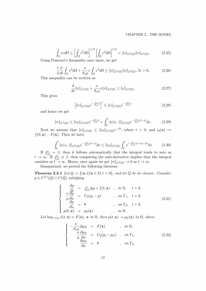
vanishes as t→∞. Hence, once again we get ‖v‖L2(Ω) → 0 as t→∞.Summarized, we proved the following theorem:

Theorem 2.2.1 Let Q := (x, t)|x ∈ Ω, t > 0, and let Q be its closure. Considerp ∈ C2,1(Q) ∩ C(Q) satisfying

∂p

∂t= κ

Sεµ∆p+ f(t,x) , in Ω, t > 0,

κ

µ

∂p

∂n= Cb(pb − p) , on Γ1, t > 0,

∂p

∂n= 0 , on Γ2, t > 0,

p(0,x) = p0(x) , in Ω.

(2.31)

Let limt→∞ f(t,x) = F (x), x in Ω, then p(t,x)→ pE(x) in Ω, where− κ

Sεµ∆pE = F (x) , in Ω,

κ

µ

∂pE∂n


∂pE∂n

= 0 , on Γ2.

(2.32)

12

Chapter 3

The Numerical Method

A patient-specific finite-element model was developed using the poroelastic materialmodel described in section 2.1. An estimated normal patient brain mesh withtriangular elements was generated by processing both the patient’s CT data anda standard MRI based brain atlas (see section 3.4). This mesh was used to findthe steady-state solution in the undeformed brain, which gave an estimation ofthe strain and pressure distribution in the patient’s pre-TBI brain. The estimatednormal patient brain was used as a starting state for the post-TBI simulation, duringwhich prescribed displacement was used to model the deformation imposed by thehematoma.

All of the image processing and simulations were run on a computer with thefollowing specifications:

Processor: Two Intel Xeon E5620 (Quad Core, 2.40 GHz, 12MB Cache, 5.86 GT/sIntel QPI)

Operating system: Windows 7 Professional (64-bit)

RAM: 24GB (6x4GB) 1333MHz DDR3 ECC RDIMM

Graphics card: 2 GB AMD FirePro V5900

The following assumptions and simplifications were made in this model:

1. White matter and grey matter were combined into a single class of "braintissue" with parameter values between those of the white and grey tissues.This was done to focus on how the use of prescribed deformation affects themodel without the complication of multiple tissues.

2. The tentorium and falx were modeled as continuous brain tissue. In realitythey are deep folds into which fluid can potentially flow.

3. The patient is in the supine position, and was a previously healthy adult.These are the conditions used for measurement of ICP in the literature.

13

CHAPTER 3. THE NUMERICAL METHOD

4. Gravity was not incorporated into the model.

5. The choroid plexus was modeled as a point, rather than a structure thatoccupies a certain volume.

3.1 Finite-element methodCOMSOL Multiphysics 4.2a [7] was used to construct the poroelastic model de-scribed above. It was started with the following command:

comsol.exe -mpmode owner -blas mkl

The parameter mpmode owner sets the multiprocessor mode to owner, which,according to the COMSOL Installation and Operations Guide [6], "provides thehighest performance in most cases." The blas mkl parameter specifies the MathKernel Library for basic linear algebra operations (optimized for Intel processors).

The solid phase was modeled using the Linear Elastic Material Model in theSolid Mechanics module with quadratic discretization of the displacement field.The equations of the liquid phase were modeled using the Coefficient Form of thePDE module with Lagrange shape functions and quadratic element order.

A mesh generated from medical images was imported (see figure 3.1 and section3.4). A two-step study was run. First a deformation-free steady-state solution wasfound, which is an estimate of the normal (pre-TBI) brain. This was the inputto the second step, a discrete-time simulation with a constant rate of deformationof the surface where the hematoma grows, starting from zero deformation to thefinal deformation found in the imaging step. This was accomplished by alteringthe magnitude of the prescribed displacement vector with a scaling factor, andlinearly increasing the value of the scale factor over time. The discrete-time had15 iterations of 1000 seconds, which was pre-set (i.e. not automatically chosen by

(a) Top (b) Side (c) Front

Figure 3.1: Mesh imported into COMSOL from the top, side and front views.

14

3.2. WEAK FORM

COMSOL). A similar study was also done by replacing the discrete-time simulationwith a steady-state hematoma simulation.

3.2 Weak formFirst we find the weak form of the solid phase. Firstly, (2.4) is rewritten in thefollowing way:

G∇2ui + G

(1− 2ν)∂

∂xi(∇ · u)− α ∂p

∂xi= 0 (3.1)

For each of the three spatial components (i ∈ x, y, z) we multiply (3.1) by atest function ηi. Because of the non-homogeneous essential boundary conditions,we specify that the test function satisfies the homogeneous essential boundary con-ditions, so η(x) ∈ Σ = η | η|Γ3 = 0 Then we integrate over the domain Ω:∫

Ω

G∇2ui + G

(1− 2ν)∂

∂xi(∇ · u)− α ∂p

∂xi

ηidΩ = 0 (3.2)

Using integrations by parts we find that∫Ω

∂

∂xi(∇ · u)ηidΩ =

∫Γ∇ · uniηidΓ−

∫Ω∇ · u∂ηi

∂xidΩ (3.3)

where ni is the i-th component of the surface normal n. Similarly, using Green’sTheorem we find∫

Ω∇2uiηidΩ =

∫Γ∇ui · nηidΓ−

∫Ω∇ηi · ∇uidΩ. (3.4)

Substitution of (3.3) and (3.4) into (3.5) yields:

∫Ω

G∇ηi · ∇ui + G

(1− 2ν)∇ · u∂ηi∂xi

+ α∂p

∂xiηi

dΩ = −

∫Γ∇ · uni +∇ui · n ηidΓ

(3.5)where application of the boundary condition (2.9) and η|Γ3 = 0 leads to the

following expression of the boundary integral:

∫Γ∇ · uni +∇ui · n ηidΓ =

∫Γ1∪Γ2

∇ · f(x)ni +∇fi(x) · n ηidΓ (3.6)

Now we find the weak form of the liquid phase equation, (2.8), which we reorderin the following way:

Sε∂p

∂t+ α

∂

∂t∇ · u = κ

µ∇2p+Qs (3.7)

First we multiply (3.7) by a test function ηp, then integrate over the domain Ω:

15


∫Ω

Sε∂p

∂t+ α

∂

∂t∇ · u

ηpdΩ =

∫Ω

κ

µ∇2p+Qs

ηpdΩ. (3.8)

Using Green’s Theorem we find that∫Ω∇2pηpdΩ =

∫Γηp∇p · ndΓ−

∫Ω∇ηp · ∇pdΩ (3.9)

Substitution of (3.9) into (3.8) and application of boundary conditions (2.11)and (2.12) yields:

∫Ω

Sε∂p

∂t+ α

∂∇ · u∂t

ηpdΩ =

∫Ω

Qsηp −

κ

µ∇ηp · ∇p

dΩ +

∫Γ1Cb(pb − p)ηpdΓ.

(3.10)

3.3 Time integrationOnce basis functions are applied to the weak form of the fluid equations, (3.10) maybe expressed a system of equations with the form:

Mp∂p

∂t+Mε

∂∇ · u∂t

= Sp+ f. (3.11)

The COMSOL simulations used Euler-Backwards implicit time integration, whichcan be expressed as:

Mppn+1 − pn

∆t +Mε∇ · un+1 −∇ · un

∆t = Spn+1 + fn+1, (3.12)

where n + 1 corresponds to the current time step and n corresponds to theprevious time step. If we solve the equation for the solid phase before the liquidphase, then ∇ · un+1 is known and we can rearrange (3.12) in the following way:

pn+1 = pn +M−1p

Mε(∇ · un −∇ · un+1) + ∆t(Spn+1 + fn+1)

(3.13)

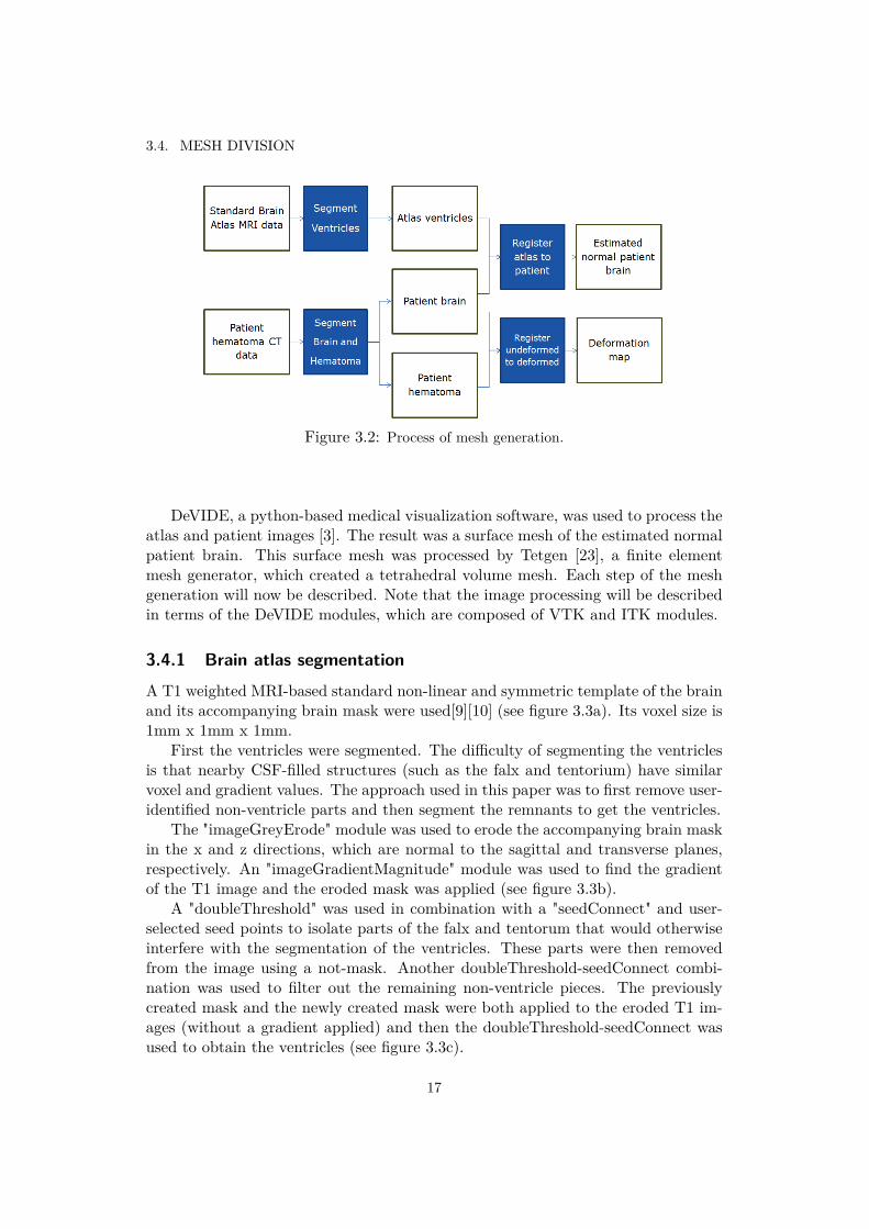
3.4 Mesh divisionIn order to run a patient-specific simulation, it was first necessary to derive a meshof the estimated normal brain according to the patient’s unique head geometry.To estimate the pre-TBI brain, an MRI-based atlas was first segmented to obtainthe shape of the ventricles and the SAS. Similarly, the patient’s CT image wassegmented to find the shape of the patient’s brain. Image registration was used toconstruct an estimated normal patient brain and to find a deformation map thatdescribes how the hematoma deforms the brain’s surface. Figure 3.2 shows the flowof the image processing involved in mesh generation.

16

3.4. MESH DIVISION

Figure 3.2: Process of mesh generation.

DeVIDE, a python-based medical visualization software, was used to process theatlas and patient images [3]. The result was a surface mesh of the estimated normalpatient brain. This surface mesh was processed by Tetgen [23], a finite elementmesh generator, which created a tetrahedral volume mesh. Each step of the meshgeneration will now be described. Note that the image processing will be describedin terms of the DeVIDE modules, which are composed of VTK and ITK modules.

3.4.1 Brain atlas segmentation

A T1 weighted MRI-based standard non-linear and symmetric template of the brainand its accompanying brain mask were used[9][10] (see figure 3.3a). Its voxel size is1mm x 1mm x 1mm.

First the ventricles were segmented. The difficulty of segmenting the ventriclesis that nearby CSF-filled structures (such as the falx and tentorium) have similarvoxel and gradient values. The approach used in this paper was to first remove user-identified non-ventricle parts and then segment the remnants to get the ventricles.

The "imageGreyErode" module was used to erode the accompanying brain maskin the x and z directions, which are normal to the sagittal and transverse planes,respectively. An "imageGradientMagnitude" module was used to find the gradientof the T1 image and the eroded mask was applied (see figure 3.3b).

A "doubleThreshold" was used in combination with a "seedConnect" and user-selected seed points to isolate parts of the falx and tentorum that would otherwiseinterfere with the segmentation of the ventricles. These parts were then removedfrom the image using a not-mask. Another doubleThreshold-seedConnect combi-nation was used to filter out the remaining non-ventricle pieces. The previouslycreated mask and the newly created mask were both applied to the eroded T1 im-ages (without a gradient applied) and then the doubleThreshold-seedConnect wasused to obtain the ventricles (see figure 3.3c).

17


(a) Original image (b) Masked gradient (c) Result

Figure 3.3: Ventricle segmentation of the T1-weighted MRI atlas (transverse slices). (a)The original T1 image. The darkest regions in the brain tissue are the ventricles. (b) Thegradient of the original image with an eroded brain mask applied. The gradient highlightsthe interfaces between material types. (c) Surface mesh of the segmented ventricles (purple)and removed portions (yellow and blue).

3.4.2 Patient image segmentation

The patient image used in this study is a CT scan with voxel size 0.41mm x 0.41mmx 0.63mm showing a SDH on the left side of the brain with compressed ventricles,as seen in figure 3.4a. Unlike the atlas, the patient image did not come with abrain mask, so the first step was to segment the brain from the eyes, skull and

(a) Hematoma and ventricles (b) Eye socket connection

Figure 3.4: CT scan of a patient with an SDH on the left side of the brain. (a) Thehematoma is outlined in red and the (deformed) ventricles in yellow. (b) The eye socketsare not separated from the brain cavity by bone. The tissue appears to be continuous.

18

3.4. MESH DIVISION

(a) Resampled and thresholded image (b) Image gradient with thresholding high-lighted

(c) Separated tissue regions

Figure 3.5: Segmentation of patient brain. (a) Image with thresholded tissue. (b) Gradientof image with filtered borders highlighted in green. (c) Surface data of brain (purple) andother tissue regions (red).

other non-brain tissues. Figure 3.4b shows that the eye and brain tissue seems tobe continuous through the eye socket.

The image is fairly grainy, so an "imageGaussianSmooth" filter was applied. Inorder to speed up the image processing, the number of voxels was reduced using"resampleImage." Brain tissue and CSF were segmented by using "doubleThreshold"

19


Figure 3.6: 3D visualization of segmentation hematoma.

with range 1 to 100 Hounsfield units (HU), seen in figure 3.5a. Interfaces betweentissues were found using "imageGradientMagnitude". Boundaries external to thebrain were selected using "doubleThreshold" (figure 3.5b).

Notice that the left eye remained connected to the brain. A "closing" modulefilled the gap. The module dilates then erodes the non-zero regions. This resultsin boundaries that completely enclose the brain without any openings to non-brainregions. The segmented boundaries were removed from the filtered image.

At this point, the brain was separated from the rest of the tissues, but the re-maining non-brain tissues needed to be removed. In an emergency setting, imageprocessing and simulation must be quick and simple. Thus, minimal user interactionis desired. To automatically determine which of the tissue regions was the brain, themask was converted to surface data and the one with the most nodes was chosen.First, however, a few layers of zero-valued voxels were added to the bottom side ofthe image to disconnect the non-zero voxels from the edge of the image. When theyare in contact, the surface mesh remains open. For this, the "CodeRunner" mod-ule used the vtkCubeSource, vtkPolyDataToImageStencil, vtkImageMathematics,vtkImageStencil and vtkImageMask filters. The "contour" and "wsMeshSmooth"modules transformed the image data into surface meshes and the "vtkPolyData-ConnectivityFilter" was used to choose the largest region (figure 3.5c).

The surface data of the brain was converted back into an image with a combi-nation of vtkPolyDataToImageStencil, vtkImageMathematics, vtkImageStencil andvtkImageMask. The "opening", "closing" and "imageFillHoles" filters were used to

20

3.4. MESH DIVISION

(a) Front view (b) Side view

Figure 3.7: Landmark positioning: 1) On the middle of the surface of the cerebellum inthe back of the brain, 2 and 3) on the tips of the right and left temporal lobes, respectively,4) The top-center of the brain surface approximately where the parietal and frontal lobesmeet.

ensure that the brain mask was smooth, closed and had no holes. The final imagewas saved to file for later use.

Next the hematoma was segmented from the patient scan (figure 3.6). Firstly,the image was masked by the brain mask, resampled and smoothed. A "dou-bleThreshold" was used to filter voxels in the range of 45 to 90 HU (correspondingto blood), then "imageFillHoles" was applied to fill holes in the hematoma. The seg-mented hematoma was dilated slightly, then a surface mesh was created. As withthe brain mask, "vtkPolyDataConnectivityFilter" was used to select the largest con-nected part (thus ignoring small fragments), then the surface mesh was convertedto image data and written to file.

3.4.3 Registration

To estimate the patient’s pre-TBI brain, the segmented atlas was combined withthe patient brain mask. Four source landmark points were chosen on the atlas. Thecorresponding target landmark points were chosen on the patient (see figure 3.7).The "landmarkTransform" module was used to calculate an affine transformationfor the atlas, then applied using "transformImageToTarget". The patient’s SAS wasestimated by eroding the brain mask and subtracting the eroded mask from thenon-eroded mask. The transformed ventricles were added to the estimated SAS toobtain the final estimate of the patient brain, which is seen in figure 3.8.

The segmented hematoma extended into the tentorium and ran along the SSS.Both were removed for simplicity. The brain mask was eroded and applied toremove the tentorium part. A plane implicit function removed the SSS. The altered

21


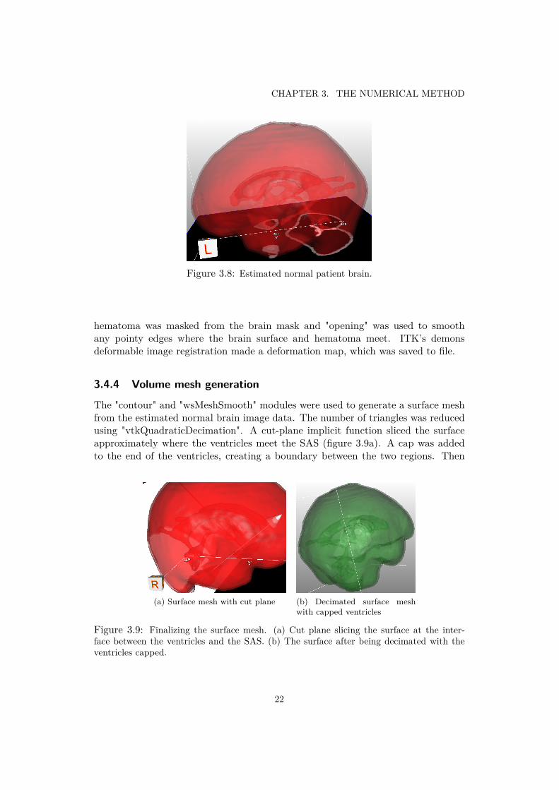
Figure 3.8: Estimated normal patient brain.

hematoma was masked from the brain mask and "opening" was used to smoothany pointy edges where the brain surface and hematoma meet. ITK’s demonsdeformable image registration made a deformation map, which was saved to file.

3.4.4 Volume mesh generation

The "contour" and "wsMeshSmooth" modules were used to generate a surface meshfrom the estimated normal brain image data. The number of triangles was reducedusing "vtkQuadraticDecimation". A cut-plane implicit function sliced the surfaceapproximately where the ventricles meet the SAS (figure 3.9a). A cap was addedto the end of the ventricles, creating a boundary between the two regions. Then

(a) Surface mesh with cut plane (b) Decimated surface meshwith capped ventricles

Figure 3.9: Finalizing the surface mesh. (a) Cut plane slicing the surface at the inter-face between the ventricles and the SAS. (b) The surface after being decimated with theventricles capped.

22

3.4. MESH DIVISION

the cut surfaces were reassembled (figure 3.9b). A text file was created with thedeformation information of each node, to be used in the simulation.

Tetgen [23] was used to transform the surface mesh to a volume mesh. The ’q’option enforced a quality mesh and the ’AA’ option told tetgen to automaticallyassign domains based on connectivity. The generated mesh can be seen in figure3.10. The tetgen file was converted to an mphtxt file (COMSOL’s input format)using a custom created java program.

(a) Right side (b) Left side (c) Sagittal slice

(d) Front side (e) Back side (f) Coronal slice

(g) Top side (h) Bottom side (i) Transverse slice

Figure 3.10: Tetgen generated volume mesh.

23

Chapter 4

Simulation Results

This chapter shows the results of the finite-element simulations. The steady statesolutions are shown in section 4.1, then the solutions for deformation over time areshown in section 4.2. The remaining sections show the effect of altering variousparameters.

4.1 Steady state

The segregated solvers for both the normal and post-TBI brain converged in twoiterations, with pressure p converging in two and one iterations, respectively. Inboth cases, displacement u converged in two iterations.

Figure 4.1 displays the steady state solutions in both the normal brain andthe deformed brain. The range of values was identical (1155.8 to 1187.5 Pa), andthe coloration was approximately the same. The deformation is not shown in thepressure plots. The absolute value of the first principal strain in the normal brainand deformed brains had data ranges 0 to 0.0168 and 0 to 21.492, respectively, butwith color legend showing values from 0 to 0.2. In the normal brain, there was littlestrain, except with a slight elevation near to the walls of the ventricles. The strainin the deformed brain was elevated compared to the normal brain, and concentratedaround the walls of the ventricles, and especially near the outer surface of the frontof the frontal lobes and the back of the left temporal and occipital lobes.

The strain plots show the deformation of the brain. In the normal brain therewas no outer deformation and the ventricles had no visible deformation. In thedeformed brain, the outer deformation was subtle, but visible on the left side of thebrain. The ventricles appeared to be slightly compressed, especially on the left side.

4.2 Hematoma over 15000 seconds

From start to finish, running the hematoma study took less than eight minutes,which included building the matrices, running the steady-state normal simulation

25

CHAPTER 4. SIMULATION RESULTS

(a) Normal pressure (b) Normal strain

(c) TBI pressure (d) TBI strain

Figure 4.1: Transverse slices of the stationary solutions. (a) The pressure distribution inthe estimated normal brain, deformation not shown (data range: 1155.8 to 1187.5 Pa ). (b)The absolute value of the first principal strain in the estimated normal brain, deformationshown (data range: 0 to 0.0168). (c) The pressure distribution in the deformed brain,deformation not shown (data range:1155.8 to 1187.5 Pa ). (d) The absolute value of thefirst principal strain in the deformed brain, deformation shown (data range: 0 to 21.492,color legend showing values from 0 to 0.2).

26

4.2. HEMATOMA OVER 15000 SECONDS

(a) 0 s (b) 5000 s (c) 10000 s (d) 15000 s

Figure 4.2: Transverse slices of the stationary hematoma brain showing pressure over 15000seconds.

and running the discrete-time simulation with 15 time-steps of 1000 seconds. Therewere 393654 degrees of freedom.

Figure 4.2 shows the pressure distribution changing over a time period of 0 to15000 seconds. The pressure rose over time in all parts of the brain, but especiallyon the left side, with concentrations in the left frontal and parietal lobes. As defor-mation increased, the pressure in the SAS remained lower than in the brain. Thehighest pressure reached was nearly 2900Pa ' 21.75mmHg. At 15000 seconds, thelowest pressure was around 1800Pa ' 13.50mmHg.

(a) 0 s (b) 5000 s (c) 10000 s (d) 15000 s

Figure 4.3: Transverse slices of the stationary hematoma brain showing first principalstress over 15000 seconds.

27


(a) (b)

(c) (d)

Figure 4.4: (a) Intracranial pressure as a function of time for various scale factors, (b)Intracranial pressure as a function of scale factor at 15000s. (c) Maximum pressure as afunction of time for various scale factors, (d) Maximum pressure as a function of scale factorat 15000s.

Figure 4.3 shows the absolute value of the first principal strain changing over atime period of 0 to 15000 seconds. The strain generally rose everywhere, but in theright part of the brain the change didn’t appear to be significant, except in and nearthe SAS. The greatest increases were in the left side of the brain, with the highestconcentrations in the front of the frontal lobes and the back parts of the temporaland occipital lobes. The strain was also elevated around the ventricle walls and inthe middle of the frontal and parietal lobes.

28

4.3. HEMATOMA SCALE FACTOR PARAMETER STUDY

(a) 1.0 (b) 2.0 (c) 3.0

Figure 4.5: Percent of cortical cell death at 15000s for hematoma scale factors (a) 1.0, (b)2.0 and (c) 3.0.

4.3 Hematoma scale factor parameter study

The magnitude of deformation due to hematoma was multiplied by a scaling factor.The time-based study was repeated with factors from zero to three. ICP (measuredin the lateral ventricles) is plotted over time and scale factor in figures 4.4a and4.4b, respectively. For scale factors between 0.5 and 3.0, ICP increased steeply in

(a) Strain (b) Strain rate (c) Strain

Figure 4.6: (a) Strain over time for various scale values. (b) Strain rate over time forvarious scale values. (a) Strain as a function of scale factor at 15000s.

29


(a) (b)

Figure 4.7: (a) Calculation of cortical cell death at a point with high pressure values overtime for various scale values. (b) Correlation between scale factor and cortical cell death.

the first few timesteps, and then leveled off to values between approximately 1500Paand 3100Pa. ICP at 15000s increased linearly with scale factor.

Maximum pressure is plotted as a function of time and scale factor in figures 4.4cand 4.4d. It increased steeply initially and started to level off as time continued. Therate of increase reduced more gradually than the rate of ICP increase. Additionally,the magnitude of maximum pressure for scale factors between 0.5 and 3.0 at 15000swere much larger than for ICP (from approximately 2000Pa to 6500Pa). As is thecase for ICP, maximum pressure at 15000s increased linearly with scale factor.

Estimated cortical cell death, calculated from (1.1), is presented for varioushematoma scale factors at a time of 15000s in figure 4.5. At a scale of 1.0, celldeath was noticeable near the surface of the brain in the frontal, temporal andoccipital lobes. At a scale factor of 2.0, cell death became noticeable in the lefthemisphere, especially around the ventricles, which became more pronounced at ascale factor of 3.0.

Measurements of strain and strain rate were taken at point in the left hemi-sphere where pressure appears to be maximal (figure 4.6) and cortical cell deathwas calculated (figure 4.7). Strain increased with time. After an initial spike, strainrate decreased with time and appeared to head towards a steady-state. Strain at15000s increased linearly with scale factor. Cell death increased over time. In allcases, higher scale factors corresponded to higher measured/calculated values.

30

4.4. DEFORMATION

(a) Reference (b) 1.00 (c) 1.50

(d) 2.00 (e) 2.50 (f) 3.00

Figure 4.8: Original and simulated brains at 15000s with various hematoma scales showingdeformation and mid-line shifts. The estimated normal mid-line is shown in blue andundeformed inner and outer surfaces are shown in green. The purple line is the approximatemid-line of the real (reference) brain and the red lines show the approximate mid-lines ofthe simulated brains. For all of the simulated brains (but not the reference brain), theshading shows the total displacement.

4.4 Deformation

Figure 4.8a shows deformation in the original patient brain, with estimated originalsurface locations shown in green, the estimated original mid-line shown in blueand the approximate deformed mid-line in purple. Figures 4.8b to 4.8f show the

31


deformation and corresponding mid-line shift in red. The shading shows the totaldisplacement. The shape of the simulated hematoma was much more smooth thanthe original, as was the mid-line shift.

4.5 ICP as a function of hematoma volume and infusedvolume

Image processing was used to determine the volume of the hematoma at variousscale factors (figure 4.9a). Hematoma volume increased linearly with scale factor.

(a) (b)

Figure 4.9: (a) Scale factor as a function of hematoma volume. (b) ICP as a function ofvolume of simulated infused CSF (blue), hematoma (green) and experimental infused CSF(red).

A CSF point source was chosen in the middle-back of the outer surface of theSAS and given a flow rate of 3.87mL/min to mimic the infusion experiments of Sklarand Elashvili [26]. Figure 4.9b shows the simulated infusion experiment (blue), theexperimental infusion experiment (red) and ICP plotted as a function of hematomavolume (green). The experimental data had an exponential relationship, but thesimulated results did not.

4.6 Hyper- and hypotensionThus far, the results have assumed that the patient has no health problems priorto the accident. Some health conditions, such as hyper- and hypotension could

32

4.6. HYPER- AND HYPOTENSION

(a) Pressure over pb (b) Strain over time

(c) Strain over pb: 0s (d) Strain over pb: 15000s (e) Cortical cell death over pb:15000s

Figure 4.10: Pressure, strain and cell death for a range of values of baseline pressure, pb.(a) Pressure as a function of pb. (b) Average strain and strain at a point of high pressure asa function of time for various values of pb. (c) Strain as a function of pb at 0 seconds. (d)Strain as a function of pb at 15000 seconds. In the average case the range of values is from0.05132 to 0.05138 and in the high pressure case the range of values is 0.06494 to 0.06507.In both cases, the shape is the same. (e) Cortical cell death as a function of time for variousvalues of pb at a point of high pressure at 15000 seconds.

affect the pressure and strain experienced by the patient after injury. Outflowconductance, Cb, could be a factor in intracranial hypertension, whereas baselinevenous pressure, pb, may be an indicator of systemic hypertension.

Figure 4.10 shows the effect of changing pb on pressure, strain and cortical celldeath. ICP and maximum pressure had roughly the same value at 0s, which werelower than the values at 15000s. All pressure curves appeared to be linear. ICP

33


at 15000s ranged from 1406Pa ' 10.5mmHg to 2656Pa ' 19.9mmHg. There wasalmost no variation of strain and curve shape between pb values of 250Pa and 1500Pafor both the average and high pressure cases. The high pressure curve had higherstrain and a different shape than the average curve. At 0s, both the average andhigh pressure strains increased with pb. For lower values of pb, the high pressurestrain was larger than the average strain, but then after about pb = 1350Pa, theaverage became larger than the high pressure. At 15000s, the shapes of both curveswere the same, but with different data ranges (average: 0.05132 to 0.05138, highpressure: 0.06494 to 0.06507). Cortical cell death decreased with baseline pressure.

Figure 4.11 shows the effect of changing Cb on pressure, strain and cortical celldeath. At 0s, ICP and maximum pressure had roughly the same values, which werelower than the values at 15000s. At 15000s, maximum pressure appeared to be onlyslightly higher than ICP in figure 4.11a, but the difference is more obvious in figure4.11a. The shape of all pressure curves was roughly the same. There was almost novariation of strain between Cb = 1.25e−9m4s/kg and 1.25e−11m4s/kg for both theaverage and high pressure cases. The high pressure strain at Cb = 1.25e−13m4s/kgdipped down initially, but then recovered to a shape similar to the other plottedstrains. At very small Cb, there was a noticeable difference between average and highpressure strain at both 0s and 15000s. At larger Cb, at 0s there was no noticeabledifference and at 15000s there was a large difference. At very small Cb cell deathwas quite small, but increased steeply and eventually leveled out as Cb increased.

34

4.6. HYPER- AND HYPOTENSION

(a) Pressure over Cb (b) Pressure over Cb (smallerrange)

(c) Strain over time

(d) Strain over Cb (e) Cortical cell death over Cb: 15000s

Figure 4.11: Pressure, strain and cell death for a range of values of conductance, Cb. (a)ICP and maximum pressure as a function of Cb at 0 and 15000 seconds. (b) Average strainand strain at a point of high pressure as a function of time for various values of Cb. (c)Average strain and strain at a point of high pressure as a function of Cb at 0 and 15000seconds. (d) Cortical cell death at a point of high pressure as a function of Cb at 15000seconds.

35

Chapter 5

Discussion and Conclusion

5.1 Steady state

Solving for the steady-state solutions was quite efficient, as only two iterations wererequired to solve each of the two segregated steps. In the case of solving for pressurein the post-TBI brain, the small residual in the first post-TBI step is explained byour expectation of convergence to the normal-brain solution (see section 2.2).

The behavior described in section 2.2 was reflected in the strain and pressureplots of section 4.1. As expected, the addition of deformation to the normal brain forthe steady-state TBI simulation did not affect pressure. The pressure was highestin the ventricles and then dissipated towards the SAS. Within the ventricles isthe Choroid Plexus, a fluid source. The ventricles are fluid filled cavities, so arelatively uniform pressure throughout is expected. The walls of the ventricles andthe narrow opening of the aqueduct provide resistance to the flow of fluid, whichshould cause the pressure in the ventricles to be higher than the surrounding tissue.This appeared to be the case.

At the SSS we expected outward flux, since the pressure inside (initial value of1000 Pa) was greater than the external pressure (650 Pa). The outward flux of fluidwas expected to relieve the pressure. The high fluid content of the SAS allows easyflow of fluid toward the SSS. Thus, it was expected that the pressure in the SASwas lower than the adjacent brain tissue. This was, in fact, observed.

The pressure distribution was comparable to that found by Li et al. [15]. Theyfound that pressure was highest in the ventricles and gradually reduced towardsthe SAS. The pressure they computed in the ventricles was 1183Pa, whereas in thisstudy it was 1187.5Pa. At the SAS they found a pressure of 1157Pa, whereas inthis study it was 1155.8Pa. The ranges and distributions of both studies were quitesimilar, which suggests that, in the case of the steady-state, the model operated asexpected.

The strain in the normal stationary brain was quite low and relatively uniform.In a normal, fully functioning brain, this is expected. The heightened strain in thesteady-state post-TBI brain reflected the deformation imposed by the hematoma.

37

CHAPTER 5. DISCUSSION AND CONCLUSION

The concentration of strain in the frontal, temporal and occipital lobes were notexpected. These precise locations might reflect the alteration of the hematoma inthe image processing step, where parts of the hematoma in the tentorium and SSSwere removed.

5.2 Hematoma over 15000 seconds

The evolution of pressure as the hematoma grows seemed to be, at least qualita-tively, what one would expect. Starting from a normal steady-state brain, if thetissue is compressed, with all other factors remaining the same, the pressure shouldincrease. On a microscopic level, one can imagine the pores in the brain compress-ing as the entire brain volume decreases. The fluid must push its way through thenetwork of pores before it can reach an area of low resistance and make its way tothe SSS to escape. In porous brain tissue, the available pore volume decreases fasterthan the fluid escapes, and thus the pressure increases. Being that the hematomawas on the left side of the brain, the resulting high concentration of pressure on thatside is likely accurate. The fact that the fluid-filled SAS and ventricles had lowestpressure is intuitive, since lower resistance translates to easier flow to the SSS.

The increasing strain observed on the surfaces of the frontal, temporal andoccipital lobes may have been due to the same image processing steps identifiedin the discussion of the steady-state results. It is possible that the magnitudes ofthese strains is not accurate. The gradual build-up of strain in the middle of theleft side of the brain occurs where pressure also built up. Given the co-dependenceof pressure and strain, this was expected. In the steady-state solution, the strain inthis location was not elevated, which corresponds to the convergence of the pressureto the steady-state solution. As in the steady-state, strain at each time step seemedto be concentrated around the walls of the ventricles. In both cases this reflectedthe shift in the mid-line of the brain due to the deformation of the outer surface.

5.3 Hematoma scale factor parameter study

A steady-state of ICP for all simulated hematoma scales seemed to occur by 15000s,which was not the case for cortical cell death. In fact, cell death appeared to increasesteeply at 15000s. This indicates that stabilization of ICP does not translate tostabilization of cell death. ICP seemed to stabilize faster than maximum pressure,which is likely due to low resistance to flow in the ventricles. There appeared tobe a strong relationship between strain and maximum pressure. As expected, celldeath increased with hematoma scale, and it appears to be highest in locationswhere strain is also highest. This reflects the dependence of cortical cell death onstrain and strain rate.

38

5.4. ICP AS A FUNCTION OF HEMATOMA VOLUME AND INFUSED VOLUME

5.4 ICP as a function of hematoma volume and infusedvolume

The linear relationship between hematoma volume and scale factor indicates thatchanging hematoma volume has the same effect on variables as changing hematomascale factor. The difference in shape between experimental infusion and simulatedinfusion results indicates that the poroelastic model does not accurately describethe relationship between added fluid volume and ICP. The model must be furtherexamined to determine if this will affect its viability in a clinical setting, and whetherit can be altered to be accurate. An example of a possible source of inaccuracy isthat, during a traumatic event, blood pressure likely varies in time. If the efflux offluid from the SSS is dependent on venous pressure, then the rate of fluid flux fromthe SSS should be affected. Also, increased stress can cause a change in hormonelevels, such as adrenaline, which may affect the properties of the brain. Any ofthe parameters that were assumed to be constant may, in actuality, change as thehematoma develops.

It is interesting that ICP change due to hematoma is much less than for CSFinfusion. Of course, these fluid additions are different in that CSF is free to flowwithin the brain, whereas the blood in the hematoma is not. It is difficult to saywhether this observation accurately describes what happens in the brain.

5.5 DeformationThe mid-line shift of the original brain scan was large in the front and small in theback, which may be due to the proximity of the falx to the less deformed tissue,which could provide additional structural support to this part of the brain. It couldalso be because the hematoma was situated mostly in the front of the brain. Inthe simulated results, the shape of the hematoma was much smoother and evenlydistributed than the original hematoma, which could explain why the observed mid-line shift was also more smooth from front to back of the brain. The ventricles in thesimulated results seemed to be compressed to the same degree in the left and rightsides, whereas in the real brain, the left-front seemed to be much more compressedthan the rest. Again, this could be due to some structural features in the real brainwhich were not present in the geometry of the simulated brain.

5.6 Hyper- and hypotensionNormal central venous pressure is between 3 and 8 mmHg. Changing baselinevenous blood pressure (which corresponds to systemic hypertension) had a verysmall effect on strain and estimated cortical cell death, but a large effect on ICPand maximum pressure at 15000s. One can approximate the relationship betweenpressure and the baseline venous pressure for this particular hematoma with defaultparameter values by:

39


ICP (0s) = MaximumPressure(0s) = pb + 8.9mmHg, (5.1)

ICP (15000s) = pb + 4.0mmHg, (5.2)

and

MaximumPressure(15000s) = pb + 17.2mmHg. (5.3)

The relationship between baseline venous pressure and ICP at 0s and 15000s isvisualized in figure 5.1. Systemic hypotension (pb < 3mmHg) corresponded with in-tracranial hypotension (ICP < 7Pa) at 0s and normal ICP at 15000s. All conditionsrequiring treatment occured when the patient had systemic hypertension (pb > 8mmHg). The first pb at which treatment would be considered was at 11mmHg,which was when ICP at 15000s reached 20mmHg. At this point the patient’s pre-TBI ICP was on the upper end of normal, at 15mmHg. When the baseline pressurereached 16mmHg, the patient’s pre-TBI ICP was predicted to be high enough torequire treatment, and the post-TBI ICP required aggressive treatment. Whenpb > 21mmHg, the patient’s pre-TBI condition required aggressive treatment, andthus it is unlikely that any of the conditions associated with higher baseline pres-sures would occur. At this point the patient’s baseline pressure was also way out ofthe normal range.

ICP and maximum pressure were also significantly affected by changing Cb.Intracranial hypertension occurs when ICP is above 15mmHg ' 2000Pa. Thepatient had an underlying condition of intracranial hypertension approximately

Figure 5.1: Pressure relationship and corresponding conditions and clinical actions. Nor-mal pb is between 3 and 8 mmHg (red). Normal ICP is between 7 and 15 mmHg (green forICP(0s), yellow for ICP(15000s).

40

5.7. CONCLUSION

when Cb < 7.5 × 10−13m4s/kg, which corresponds to an ICP of approximately26mmHg ' 3500Pa at 15000s. At this point, the patient would require aggressivetreatment for the hematoma. Less urgent treatment of the hematoma would beginat 20mmHg ' 2600Pa, when the patient does not have an underlying conditionof hypertension. When Cb > 1.1 × 10−13m4s/kg, the patient did not experienceintracranial hypertension at both 0 and 15000 seconds.

For all plotted values of Cb and pb, cell death at the high pressure point is atmost 0.0074%. So, when the hematoma scale factor is 1, the model predicts thatthere is very little irreparable damage to the cortex. Interestingly, an extremelysmall amount of cortical cell death is predicted to occur at very small values ofconductance, which corresponded to the patient being in a hypertensive state withdangerously high levels of ICP. These two observations contradict each other, whichsuggests that the model breaks down with very small values of conductance.

5.7 Conclusion

In this thesis, a poroelastic model of the brain was used to simulate a subduralhematoma in patient-specific geometry. Image processing was used to construct afinite-element mesh and a deformation map that describes the displacement imposedby the hematoma on the surface of the brain. These were input into a finite-elementmodel, which solved for pressure and displacement. Various parameters were studiedfor their effects on the model’s behavior.

In the steady-state studies, pressure in the normal brain and the deformed brainconverged to the same solution, as was predicted. When the hematoma was intro-duced over 15000s, the pressure climbed in a way that seemed physically plausible.Strain also seemed to behave in a plausible way, but concentrations in regions nearthe outer boundary were questionable, possibly occurring due to simplificationsmade in the geometry. It can be concluded that this model qualitatively describespressure evolution over time quite well. Further validation is required to determinewhether the model is a good predictor of strain and whether the magnitudes ofcalculated pressures is accurate.

The shape of the pressure-volume curve for the simulated results was differentfrom that of the experimental results. Also, the deformation and mid-line shift forvarious scale factors was different compared to those seen in the real brain. Thehematoma deformation map obtained in the image processing step differed greatly inshape compared to the real hematoma, which likely affected the inner deformationin the simulation. These observations highlight the need to improve the modeland validate it using corresponding patient data (such as ICP measurements frompressure probes).

An important observation was that, even though ICP converges to a steadyvalue, cortical cell death continues to rise dramatically. This highlights the need formore descriptive predictors of patient outcome. The diagnosis of TBI and predictionof upcoming effects of TBI can be vastly improved by considering other quantities

41


obtained from a poroelastic model, such as strain. The model may provide a mapof the brain upon which one can predict what regions of the brain will be hardesthit by TBI, and thus what symptoms one can expect to arise in the patient. Thiscan be used to develop targeted therapies, focusing rehabilitation efforts where theyare needed most urgently.

This study shows that a poroelastic model of the brain is a promising tool inpressure and strain prediction for patients with hematoma. Thus, it should befurther developed with the following suggestions for future directions in mind:

1. This model must be validated more extensively. It is recommended that pa-tient data that conforms to the geometric simplifications is used. Specifically,patients with subdural hematoma that does not extend into the folds of thebrain (such as the falx and tentorium) are recommended. It is preferable thatthe hematoma be easily distinguishable from the SSS. Calculated ICP shouldbe compared to that found using pressure probes. The mid-line shift predictedin the model should be compared to the actual mid-line shift and, if available,the future symptoms experienced by the patient should be compared withthose predicted based on where strain in the brain was highest.

2. When the model with simplified geometry is validated, the geometry should bealtered to also include the folds in the brain and then validated using patientdata that has hematomas extending into these folds.

3. Efforts should be made to ensure that the deformation map is smooth andthat the displacement it describes is realistic and accurate.

4. Both the image processing and simulation should be made as efficient anduser-friendly as possible.

5. A study should be done to determine the optimal mesh to be used, includingelement size, quality and type. Being that this model could be used in aclinical situation, it must be accurate and fast, so a balance must be foundbetween resolution and computation time.

42

Bibliography

[1] D.P. Agamanolis. Cerebrospinal fluid. [Online at http://neuropathology-web.org/chapter14/chapter14CSF.html; accessed 15-January-2012].

[2] Maurice A Biot. General theory of three-dimensional consolidation. Journalof Applied Physics, 12(2):155–164, 1941.

[3] Charl P. Botha and Frits H. Post. Hybrid scheduling in the DeVIDE dataflowvisualisation environment. In Helwig Hauser, Steffen Strassburger, and HolgerTheisel, editors, Proceedings of Simulation and Visualization, pages 309–322.SCS Publishing House Erlangen, February 2008. Best paper award.

[4] D.W.A. Brands, G.W.M. Peters, and P.H.M. Bovendeerd. Design and numeri-cal implementation of a 3-d non-linear viscoelastic constitutive model for braintissue during impact. Journal of Biomechanics, 37(1):127 – 134, 2004.

[5] Wikimedia Commons. File:http://en.wikipedia.org/wiki/file:gray769-en.svg.[Online; accessed 26-January-2012].

[6] Comsol. COMSOL Multiphysics Installation and Operations Guide: Version4.2a, 2011.

[7] Comsol. COMSOL Multiphysics User’s Guide: Version 4.2a, 2011.

[8] M. Czosnyka, Z. Czosnyka, O. Baledent, R. Weerakkody, M. Kasprowicz,P. Smielewski, and J.D. Pickard. Dynamics of Cerebrospinal Fluid: FromTheoretical Models to Clinical Applications. Springer New York, 2011.

[9] Vladimir Fonov, Alan C. Evans, Kelly Botteron, C. Robert Almli, Robert C.McKinstry, and D. Louis Collins. Unbiased average age-appropriate atlases forpediatric studies. NeuroImage, 54(1):313 – 327, 2011.

[10] VS Fonov, AC Evans, RC McKinstry, CR Almli, and DL Collins. Unbiasednonlinear average age-appropriate brain templates from birth to adulthood.NeuroImage, 47, Supplement 1(0):S102–S102, 2009.

[11] Intracranial Hypertension Research Foundation. What is ih? [On-line at http://www.ihrfoundation.org/intracranial/hypertension/info/C16; ac-cessed 22-January-2012].

43

BIBLIOGRAPHY

[12] J. Ghajar. Traumatic brain injury. The Lancet, 356(9233):923 – 929, 2000.

[13] Mariusz Kaczmarek, Ravi Subramaniam, and Samuel Neff. The hydromechan-ics of hydrocephalus: Steady-state solutions for cylindrical geometry. Bulletinof Mathematical Biology, 59:295–323, 1997. 10.1007/BF02462005.

[14] Xiaogai Li. Finite Element and Neuroimaging Techniques to Improve Decision-Making in Clinical Neuroscience. PhD thesis, KTH Royal Institute of Tech-nology, 2012.

[15] Xiaogai Li, Hans von Holst, and Svein Kleiven. Influences of brain tissueporoelastic constants onintracranial pressure (icp) during constant-rate infu-sion. Computer Methods in Biomechanics and Biomedical Engineering, 2012.

[16] Abousleiman Y. Mehrabian, A. General solutions to poroviscoelastic model ofhydrocephalic human brain tissue. Journal of Theoretical Biology, 291(1):105–118, 2011. cited By (since 1996) 0.

[17] Karol Miller and Kiyoyuki Chinzei. Constitutive modelling of brain tissue:Experiment and theory. Journal of Biomechanics, 30(11-12):1115–1121, 1997.

[18] Shahan Momjian and Denis Bichsel. Nonlinear poroplastic model of ventriculardilation in hydrocephalus. Journal of Neurosurgery, 109(1):100–107, 2008.

[19] B. Morrison, D. K. Cullen, and M. LaPlaca. In vitro models for biomechanicalstudies of neural tissues. In Lynne E. Bilston, editor, Neural Tissue Biome-chanics, volume 3 of Studies in Mechanobiology, Tissue Engineering and Bio-materials, pages 247–285. Springer Berlin Heidelberg, 2011.

[20] W.L. Nowinski. Introduction to Brain Anatomy. Springer New York, 2011.

[21] Scott Polzin. Meninges, 2005. [Online athttp://www.encyclopedia.com/doc/1G2-3435200219.html; accessed 26-January-2012].

[22] Thibault P. Prevost, Asha Balakrishnan, Subra Suresh, and Simona Socrate.Biomechanics of brain tissue. Acta Biomaterialia, 7(1):83 – 95, 2011.

[23] H. Si. Tetgen: a quality tetrahedral mesh generator and three-dimensionaldelaunay triangulator, user’s manual. 2006.

[24] S. Sivaloganathan, M. Stastna, G. Tenti, and J.M. Drake. Biomechanics ofthe brain: A theoretical and numerical study of biot’s equations of consolida-tion theory with deformation-dependent permeability. International Journalof Non-Linear Mechanics, 40(9):1149 – 1159, 2005.

[25] S. Sivaloganathan, M. Stastna, G. Tenti, and J.M. Drake. A viscoelastic ap-proach to the modelling of hydrocephalus. Applied Mathematics and Compu-tation, 163(3):1097 – 1107, 2005.

44

[26] F. H. Sklar and I. Elashvili. The pressure-volume function of brain elasticity.Physiological considerations and clinical applications. J. Neurosurg., 47(5):670–679, Nov 1977.

[27] Ian Sobey and Benedikt Wirth. Effect of non-linear permeability in a spheri-cally symmetric model of hydrocephalus. Mathematical Medicine and Biology,23(4):339–361, 2006.

[28] L. A. Steiner and P. J. D. Andrews. Monitoring the injured brain: Icp and cbf.British Journal of Anaesthesia, 97(1):26–38, 2006.

[29] Ventikos Y. Tully, B. Cerebral water transport using multiple-network poroe-lastic theory: Application to normal pressure hydrocephalus. Journal of FluidMechanics, 667:188–215, 2011. cited By (since 1996) 0.

[30] J. van Kan, A. Segal, and F. Vermolen. The heat- or diffusion equation. Nu-merical Methods in Scientific Computing (VSSD), 2008.

[31] Herbert F. Wang. Theory of Linear Poroelasticity with Applications to Geome-chanics and Hydrogeology. Princeton University Press, 2000.

[32] Wikipedia. Subdural hematoma — Wikipedia, the free encyclopedia, 2011.[Online at http://en.wikipedia.org/wiki/Subdural_hematoma; accessed 15-January-2012].

[33] Wikipedia. Epidural hematoma — Wikipedia, the free encyclopedia, 2012.[Online at http://en.wikipedia.org/wiki/Epidural_hematoma; accessed 15-January-2012].

45

TRITA-CSC-E 2012:031 ISRN-KTH/CSC/E--12/031-SE

ISSN-1653-5715

www.kth.se

A Patient-Specific Poroelastic Model of a Brain with a ... · A Patient-Specific Poroelastic Model...

Documents

Transcript of A Patient-Specific Poroelastic Model of a Brain with a ... · A Patient-Specific Poroelastic Model...