ORIGINAL PAPER - PRODUCTION ENGINEERING

A numerical study on horizontal hydraulic fracture

J. Zhang • F. J. Biao • S. C. Zhang •

X. X. Wang

Received: 4 November 2010 / Accepted: 23 November 2011 / Published online: 21 December 2011

� The Author(s) 2011. This article is published with open access at Springerlink.com

Abstract A 3D non-linear fluid–solid coupling model for

horizontal fracture of vertical well was established with the

ABAQUS code. The wellbore, cement casing, perforation,

pay layer and barriers were included in the model. Fluid–

solid coupling elements were used to describe the behavior

of formation stress–seepage flow coupling; pore pressure

cohesive elements were employed to simulate the process

of fracture initiation and propagation in formation. A typ-

ical horizontal fracturing process of a vertical well of

Daqing Oilfield, China was simulated with the model. All

the concerned parameters in simulation were taken from

the field measurements. The simulated bottom-hole pres-

sure evolution is consistent with the data measured from

the field. The configurations of the fracture and porous

pressure distributions in the fracture are presented and

discussed.

Keywords Fracture propagation � Horizontal fracture �Non-linear model � Fluid–solid coupling � Cohesive

element

Introduction

Hydraulic fracturing has been one of the most frequently

implemented techniques for stimulating production of oil/

gas reservoirs for several decades (Sneddon 1946).

Common water-based fracturing fluid with chemical

additives is pumped at high rate and pressure into the

formation during hydraulic fracturing process. When the

pumping pressure exceeds the strength of the formation

rock, fractures are induced and propagated into the for-

mation, and then the propping agent is pumped into the

fractures to keep them from closing after pumping pressure

is released. Therefore, a man-made passage with high

conductivity is constructed and hydrocarbon can flow into

the well from the low-permeability formation (Economides

and Nolte 2000).

Horizontal or vertical fractures of vertical wells may be

developed depending on the factors such as depth of the

well, distributions of in situ stresses and lithological

parameters in formation. Fractures usually propagate per-

pendicular to the minimum principal stress. At shallow

depths, the minimum principal stresses correspond to the

overburden; therefore, horizontal fractures are constructed

(Settari and Michael 1986). Numerical simulations of

vertical fractures have been studied by many authors

(Morales and Abou-Sayed 1989; Boone and Detournay

1990) and reviewed (Fragachan et al. 1993). Most of the

models fall into pseudo 3-dimension (p-3D) and are suc-

cessful in design and performances of hydraulic fractures.

Results of microseismic imaging show that fracture ori-

entation is related to thrust fault near the wellbore. A

horizontal fracture could be formed below the fault

(Maxwell et al. 2009). Engineering practices of Daqing

Oilfield, China show that many of the hydraulic fractures

are horizontal in areas of remained reserves. Significant re-

stimulation could be gained from horizontal hydraulic

fracturing (Schneider et al. 2007), but studies on mecha-

nism and numerical simulation of horizontal fractures are

rarely founded in the literature to our knowledge. A quasi

static radial model of horizontal fracture was proposed

J. Zhang (&) � S. C. Zhang

School of Petroleum Engineering,

China University of Petroleum, Beijing 102200, China

e-mail: zhj718@126.com

F. J. Biao � X. X. Wang

Department of Modern Mechanics,

University of Science and Technology of China,

Hefei 230026, China

123

J Petrol Explor Prod Technol (2012) 2:7–13

DOI 10.1007/s13202-011-0016-4

(Sneddon 1946). The relationship among width, radius and

pressure in the fracture was presented, but flow and variation

of pressure in the fracture as well as leak off across the

fracture walls were not considered in the model. Interference

among horizontal fractures of multi-pay layer reservoirs was

studied (Zhang and Zhang 2004). However in the model

plan, strain assumption was made, the length of the fracture

was pointed to be a fixed value and the loading applied on the

fracture walls distributed force but not fluid pressure.

In the present paper, a 3D non-linear fluid–solid coupling

model for horizontal fracture was established with the

ABAQUS code. The wellbore, cement casing, pay layer,

barriers and perforations were included in the model. Fluid–

solid coupling elements were used to describe the behavior

of formation stress–seepage flow coupling; pore pressure

cohesive elements based on damage mechanics were

employed to simulate the process of fracture initiation and

propagation. A typical horizontal fracturing process of a

vertical well in the Daqing Oilfield, China was simulated

with the model. The simulated results show that the evolution

of the bottom-hole pressure matches the data measured from

the field very well. The correctness and reliability of the

proposed model is validated. The horizontal fracture/con-

figurations as well as porous pressure distributions in the

fracture are also presented and discussed.

Mathematical physics model

Hydraulic fracturing can be regarded as two physical pro-

cesses: one is the fluid field in the well and fractures; the

other is the stress–seepage flow coupling field in formation.

The two processes are connected by fluid exchange and

interaction of pressure on the fracture walls.

Governing equations of stress–seepage flow coupling

field in formation

In the current configuration, the equilibrium equation of

porous formation can be written as (Zienkiewicz and

Taylor 2005)Z

v

ð�r � pwIÞd_edV ¼Z

s

t � dvdS þZ

v

f � dvdV ð1Þ

where �r, pw, d_e, dv, t and f are the effective stress matrix, pore

pressure, virtual strain rate matrix, virtual velocity vector,

surface force vector and volume force vector, respectively.

The effective stress couples solid deformation with fluid

flow by the following formulation (Economides and Nolte

2000)

�r ¼ r � pwI ð2Þ

where r is the stress caused by solid deformation.

Continuity equation of seepage flow considering large

deformation of porous formation is (Malvern 1969)

1

J

o

otðJqwnwÞ þ

o

ox� ðqwnwvwÞ ¼ 0 ð3Þ

where J and x are the rate of volume dilatation and space

vector, respectively; qw, nw and vw are fluid density,

porosity and seepage velocity, respectively.

The kinetics equation is the Darcy’s law in the following

form (Marino and Luthin 1982)

vw ¼ � 1

nwgqw

k � opw

ox� qwg

� �ð4Þ

where k and g are permeability matrix and gravity accel-

eration vector, respectively.

Flow equations of fluid in fractures

The flow of proppant-laden fluid in the fracture is assumed

to be incompressible Newtonian fluid and can be resolved

as a tangential component along the cohesive element walls

and a normal component across the cohesive element walls,

respectively. The tangential one can be expressed as (Dean

and Schmidt 2008)

q ¼ t3

12lrp ð5Þ

where q, t, l and p are the vector of volume flow rate along

the cohesive element walls per tangential unit length, the

opening thickness of the cohesive elements, the coefficient

of viscosity of fracturing liquid in the cohesive elements

and fluid pressure in the cohesive elements, respectively.

The normal component represents speed of fluid flowing

in or out the walls of the cohesive elements. That is the

filtration rate of fracturing liquid in engineering and

expressed as (Hagoort et al. 1978)

qt ¼ ctðpi � ptÞqb ¼ cbðpi � pbÞ

(ð6Þ

where qt and qb are the volume flow rate across the top and

bottom walls of the cohesive elements, respectively; ct and

cb are the filtration coefficients of the top and bottom walls

of the cohesive elements, respectively; pt and pb are the

pore pressures at the top and bottom walls, respectively;

and pi is the fluid pressure along the middle plan of

cohesive elements.

Damage model of cohesive element

Initiation and extension of fracture are simulated with the

cohesive element. The damage initiation of the formation

can be expressed by the following criterion formula in

cohesive element (Camanho and Davila 2002)

8 J Petrol Explor Prod Technol (2012) 2:7–13

123

rnh ir0

n

� �2

þ rs

r0s

� �2

þ rt

r0t

� �2

¼ 1 ð7Þ

where rn is the normal stress, rs and rt are the tangential

stresses, and r0n is the intensity of tension of formation. r0

s

and r0t are the threshold stresses of tangential damage. The

symbol\[denotes that only tensile stress could make the

cohesive element damaged.

For simulating degeneration of elastic modulus of

cohesive element after damage initiated as expressed in Eq.

(7), the following linear damage evolution rule is adopted.

E ¼ ð1 � dÞ � E0 ð8Þ

where E0 and E are the initial element elastic modulus

(without damage) and damaged element elastic modulus,

respectively, and d is the damage factor which can be

calculated with the following formula (Turon et al. 2006)

d ¼Zdf

m

dam

reffddGC � G0

ð9Þ

where reff and d are the effective tensile stress and corre-

sponding strain, respectively. G0 and GC are the elastic

strain energy at damage initiation and at breaking of the

element, respectively.

Finite element discretization and the simulation model

The deformation, strain, stress and the fluid seepage in the

formation during hydraulic fracturing are described by Eqs.

(1)–(5) which couple each other and are highly non-linear.

A corresponding incremental finite element formula was

derived in detail (Zhang et al. 2010). The final expression

of the formula and the meanings of the variables in the

formula are listed in the following form

K LH þ aMDt S þ aNDt

� �DðuÞnþ1

DðpwÞnþ1

� �

¼ FV � MðuÞn � NðpwÞn

� �Dt ð10Þ

where D(u)n?1 and D(pw)n?1 are incremental displace-

ments and incremental pore pressure, respectively. The

submatrices in the left side of the formula and load vector

in the right side are complicatedly related to the current

deformation and pressure.

The incremental finite element formula is solved with

the well-known Newton–Raphson iteration scheme. The

tolerance value of iteration residual in each increment is set

as 0.5% of the force.

The eight node hexahedron elements are used for

describing deformation and seepage in formation. There

are four nodal unknowns at each node, i.e., incremental

displacements in three directions of the Cartesian coordi-

nate system and incremental pore pressure. The plan

cohesive elements with six nodal pairs are adopted to

simulate the fracture initiation and propagation.

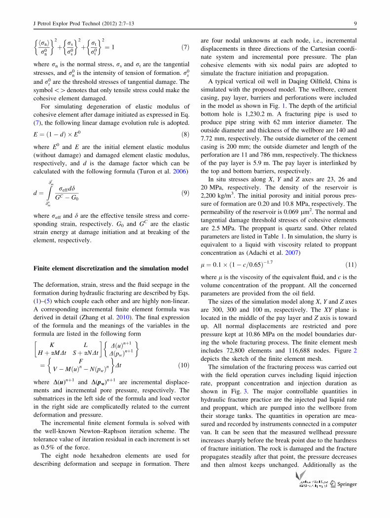
A typical vertical oil well in Daqing Oilfield, China is

simulated with the proposed model. The wellbore, cement

casing, pay layer, barriers and perforations were included

in the model as shown in Fig. 1. The depth of the artificial

bottom hole is 1,230.2 m. A fracturing pipe is used to

produce pipe string with 62 mm interior diameter. The

outside diameter and thickness of the wellbore are 140 and

7.72 mm, respectively. The outside diameter of the cement

casing is 200 mm; the outside diameter and length of the

perforation are 11 and 786 mm, respectively. The thickness

of the pay layer is 5.9 m. The pay layer is interlinked by

the top and bottom barriers, respectively.

In situ stresses along X, Y and Z axes are 23, 26 and

20 MPa, respectively. The density of the reservoir is

2,200 kg/m3. The initial porosity and initial porous pres-

sure of formation are 0.20 and 10.8 MPa, respectively. The

permeability of the reservoir is 0.069 lm2. The normal and

tangential damage threshold stresses of cohesive elements

are 2.5 MPa. The proppant is quartz sand. Other related

parameters are listed in Table 1. In simulation, the slurry is

equivalent to a liquid with viscosity related to proppant

concentration as (Adachi et al. 2007)

l ¼ 0:1 � ð1 � c=0:65Þ�1:7 ð11Þ

where l is the viscosity of the equivalent fluid, and c is the

volume concentration of the proppant. All the concerned

parameters are provided from the oil field.

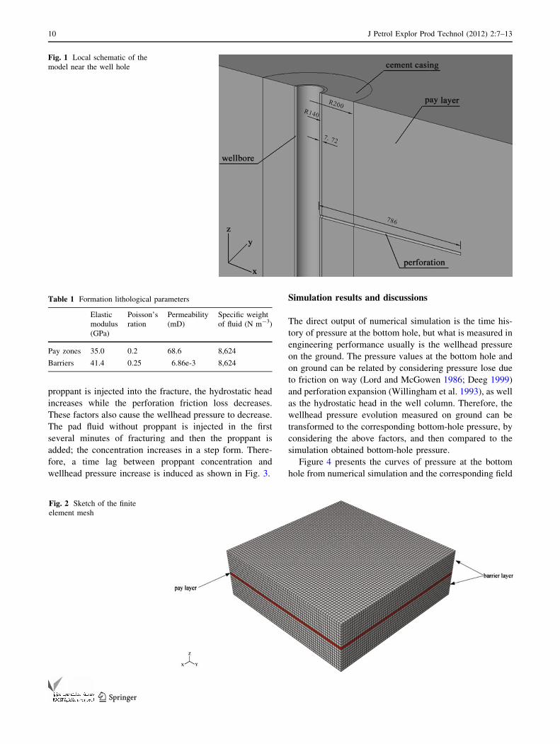
The sizes of the simulation model along X, Y and Z axes

are 300, 300 and 100 m, respectively. The XY plane is

located in the middle of the pay layer and Z axis is toward

up. All normal displacements are restricted and pore

pressure kept at 10.86 MPa on the model boundaries dur-

ing the whole fracturing process. The finite element mesh

includes 72,800 elements and 116,688 nodes. Figure 2

depicts the sketch of the finite element mesh.

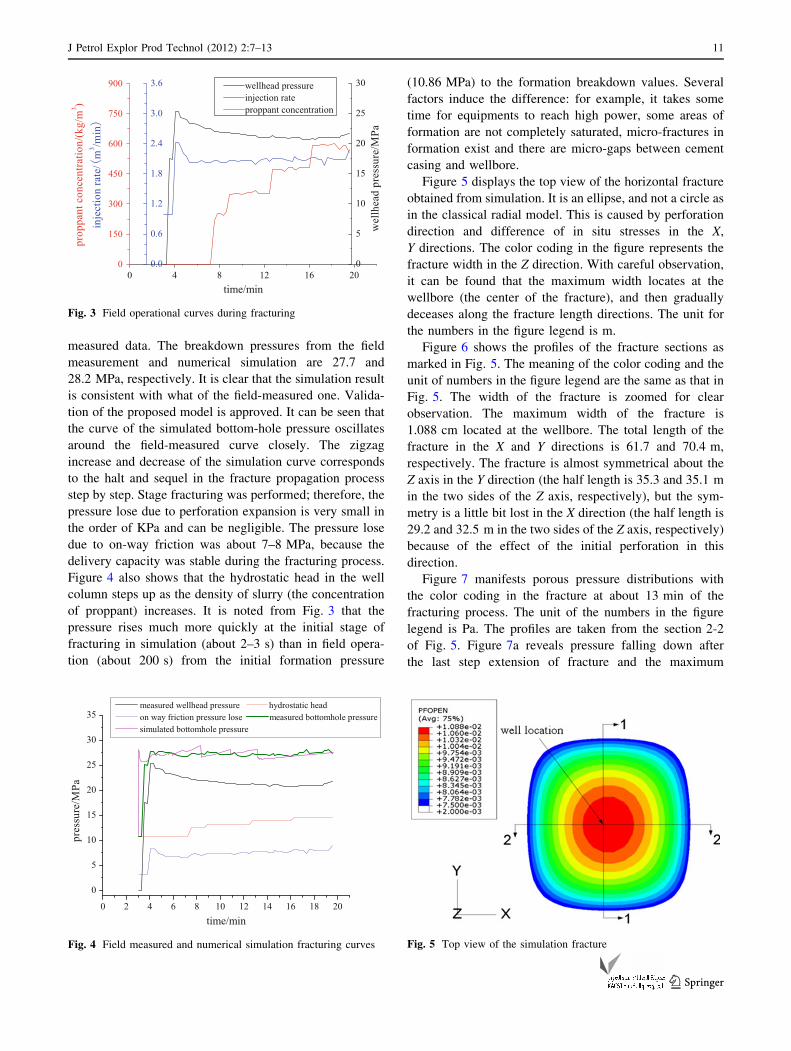
The simulation of the fracturing process was carried out

with the field operation curves including liquid injection

rate, proppant concentration and injection duration as

shown in Fig. 3. The major controllable quantities in

hydraulic fracture practice are the injected pad liquid rate

and proppant, which are pumped into the wellbore from

their storage tanks. The quantities in operation are mea-

sured and recorded by instruments connected in a computer

van. It can be seen that the measured wellhead pressure

increases sharply before the break point due to the hardness

of fracture initiation. The rock is damaged and the fracture

propagates steadily after that point, the pressure decreases

and then almost keeps unchanged. Additionally as the

J Petrol Explor Prod Technol (2012) 2:7–13 9

123

proppant is injected into the fracture, the hydrostatic head

increases while the perforation friction loss decreases.

These factors also cause the wellhead pressure to decrease.

The pad fluid without proppant is injected in the first

several minutes of fracturing and then the proppant is

added; the concentration increases in a step form. There-

fore, a time lag between proppant concentration and

wellhead pressure increase is induced as shown in Fig. 3.

Simulation results and discussions

The direct output of numerical simulation is the time his-

tory of pressure at the bottom hole, but what is measured in

engineering performance usually is the wellhead pressure

on the ground. The pressure values at the bottom hole and

on ground can be related by considering pressure lose due

to friction on way (Lord and McGowen 1986; Deeg 1999)

and perforation expansion (Willingham et al. 1993), as well

as the hydrostatic head in the well column. Therefore, the

wellhead pressure evolution measured on ground can be

transformed to the corresponding bottom-hole pressure, by

considering the above factors, and then compared to the

simulation obtained bottom-hole pressure.

Figure 4 presents the curves of pressure at the bottom

hole from numerical simulation and the corresponding field

Fig. 1 Local schematic of the

model near the well hole

Table 1 Formation lithological parameters

Elastic

modulus

(GPa)

Poisson’s

ration

Permeability

(mD)

Specific weight

of fluid (N m-3)

Pay zones 35.0 0.2 68.6 8,624

Barriers 41.4 0.25 6.86e-3 8,624

Fig. 2 Sketch of the finite

element mesh

10 J Petrol Explor Prod Technol (2012) 2:7–13

123

measured data. The breakdown pressures from the field

measurement and numerical simulation are 27.7 and

28.2 MPa, respectively. It is clear that the simulation result

is consistent with what of the field-measured one. Valida-

tion of the proposed model is approved. It can be seen that

the curve of the simulated bottom-hole pressure oscillates

around the field-measured curve closely. The zigzag

increase and decrease of the simulation curve corresponds

to the halt and sequel in the fracture propagation process

step by step. Stage fracturing was performed; therefore, the

pressure lose due to perforation expansion is very small in

the order of KPa and can be negligible. The pressure lose

due to on-way friction was about 7–8 MPa, because the

delivery capacity was stable during the fracturing process.

Figure 4 also shows that the hydrostatic head in the well

column steps up as the density of slurry (the concentration

of proppant) increases. It is noted from Fig. 3 that the

pressure rises much more quickly at the initial stage of

fracturing in simulation (about 2–3 s) than in field opera-

tion (about 200 s) from the initial formation pressure

(10.86 MPa) to the formation breakdown values. Several

factors induce the difference: for example, it takes some

time for equipments to reach high power, some areas of

formation are not completely saturated, micro-fractures in

formation exist and there are micro-gaps between cement

casing and wellbore.

Figure 5 displays the top view of the horizontal fracture

obtained from simulation. It is an ellipse, and not a circle as

in the classical radial model. This is caused by perforation

direction and difference of in situ stresses in the X,

Y directions. The color coding in the figure represents the

fracture width in the Z direction. With careful observation,

it can be found that the maximum width locates at the

wellbore (the center of the fracture), and then gradually

deceases along the fracture length directions. The unit for

the numbers in the figure legend is m.

Figure 6 shows the profiles of the fracture sections as

marked in Fig. 5. The meaning of the color coding and the

unit of numbers in the figure legend are the same as that in

Fig. 5. The width of the fracture is zoomed for clear

observation. The maximum width of the fracture is

1.088 cm located at the wellbore. The total length of the

fracture in the X and Y directions is 61.7 and 70.4 m,

respectively. The fracture is almost symmetrical about the

Z axis in the Y direction (the half length is 35.3 and 35.1 m

in the two sides of the Z axis, respectively), but the sym-

metry is a little bit lost in the X direction (the half length is

29.2 and 32.5 m in the two sides of the Z axis, respectively)

because of the effect of the initial perforation in this

direction.

Figure 7 manifests porous pressure distributions with

the color coding in the fracture at about 13 min of the

fracturing process. The unit of the numbers in the figure

legend is Pa. The profiles are taken from the section 2-2

of Fig. 5. Figure 7a reveals pressure falling down after

the last step extension of fracture and the maximum

Fig. 3 Field operational curves during fracturing

Fig. 4 Field measured and numerical simulation fracturing curves Fig. 5 Top view of the simulation fracture

J Petrol Explor Prod Technol (2012) 2:7–13 11

123

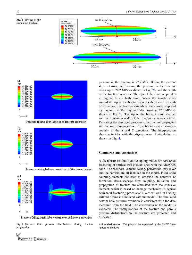
pressure in the fracture is 27.2 MPa. Before the current

step extension of fracture, the pressure in the fracture

raises up to 28.2 MPa as shown in Fig. 7b, and the width

of the fracture increases. The tips of the fracture profiles

in Fig. 7a, b are both blunt. When the tensile stress

around the tip of the fracture reaches the tensile strength

of formation, the fracture extends at the current step and

the pressure in the fracture falls down to 27.6 MPa as

shown in Fig. 7c. The tip of the fracture looks sharper

and the maximum width of the fracture decreases a little.

Repeating the described processes, the fracture propagates

step by step. Propagations of the fracture occur simulta-

neously in the X and Y directions. The interpretation

above coincides with the zigzag curve of simulation as

shown in Fig. 4.

Summaries and conclusions

A 3D non-linear fluid–solid coupling model for horizontal

fracturing of vertical well is established with the ABAQUS

code. The wellbore, cement casing, perforation, pay layer

and the barriers are all included in the model. Fluid–solid

coupling elements are used to describe the behavior of

formation stress–seepage flow coupling. Initiation and

propagation of fracture are simulated with the cohesive

element, which is based on damage mechanics. A typical

horizontal fracturing process of a vertical well in Daqing

Oilfield, China is simulated with the model. The simulated

bottom-hole pressure evolution is consistent with the data

measured from the field. The correctness of the model is

validated. The configurations of the fracture and porous

pressure distributions in the fracture are presented and

discussed.

Acknowledgments The project was supported by the CNPC Inno-

vation Foundation

Fig. 6 Profiles of the

simulation fracture

Fig. 7 Fracture fluid pressure distributions during fracture

propagation

12 J Petrol Explor Prod Technol (2012) 2:7–13

123

Open Access This article is distributed under the terms of the

Creative Commons Attribution License which permits any use, dis-

tribution and reproduction in any medium, provided the original

author(s) and source are credited.

References

Adachi J, Siebrits E, Peirce A, Desroches J (2007) Computer

simulation of hydraulic fractures. Int J Rock Mech Min Sci

44:739–757

Boone TJ, Detournay E (1990) Response of a vertical hydraulic

fracture intersecting a poroelastic formation bounded by semi-

infinite impermeable elastic layers. Int J Rock Mech Min Sci

Geomech 27(3):189–197

Camanho PP, Davila CG (2002) Mixed-mode decohesion finite

elements for the simulation of delamination in composite

materials. NASA/TM-2002-211737

Dean RH, Schmidt JH (2008) Hydraulic fracture predictions with a

fully coupled geomechanical reservoir simulator. SPE Annual

Technical Conference and Exhibition, 21–24 September 2008,

Denver, Colorado, SPE 116470-MS

Deeg WFJ (1999). High propagation pressures in transverse hydraulic

fractures: cause, effect and remediation. SPE Annual Technical

Conference and Exhibition, 3–6 October 1999, Houston, Texas,

SPE 56598

Economides MJ, Nolte KG (2000). Reservoir stimulation. John Wiley

& Sons Ltd, New York, pp 80–90, 160–167

Fragachan FE, Mack MG, Nolte KG and Teggin DE (1993) Fracture

characterization from measured and simulated bottomhole

pressure. Low Permeability Reservoirs Symposium, 26–28 April

1993, Denver, Colorado, SPE 5848-MS

Hagoort J, Weatherill BD and Settari A (1978) Modeling the

propagation of waterflood-induced hydraulic fractures. 1978 SPE

Annual Fall Technical Conferences and Exhibition, Houston,

Oct 1–4, SPE 7412

Lord DL, and McGowen JM (1986) Real-time treating pressure

analysis aided by new correlation. SPE Annual Technical

Conference and Exhibition, 5–8 October 1986, New Orleans,

Louisiana, SPE 15367

Malvern LE (1969) Introduction to the mechanics of a continuous

medium. Prentice-Hall Inc, NJ, pp 207–215

Marino MA, Luthin JN (1982) Seepage and groundwater. Elsevier

Scientific Pub Co, New York, pp 27–32

Maxwell SC, Zimmer U, Gusek R, Quirk D (2009) Evidence of a

horizontal hydraulic fracture from stress rotations across a thrust

fault. SPE Prod Oper 24(2):312–319

Morales RH, Abou-Sayed AS (1989) Microcomputer analysis of

hydraulic fracture behavior with a pseudo-three-dimensional

simulator. SPE Prod Eng 4:69–74

Schneider TS, Uldrich DO, Hodge R, Barree B and Martin MW

(2007). Horizontal fracture stimulation success in the alpine

formation, North Slope, Alaska. SPE Hydraulic Fracturing

Technology Conference, 29–31 January 2007, College Station,

Texas, SPE 106050-MS

Settari A, Michael CP (1986) Development and testing of a pseudo-

three-dimensional model of hydraulic fracture geometry. SPE

Prod Eng 1(6):449–466

Sneddon N (1946) The distribution of stress in the neighborhood of a

crack in an elastic solid. Proc R Soc London A 187:229–260

Turon A, Camanho PP, Costa J, Davila CG (2006) A damage model

for the simulation of delamination in advanced composites under

variable-model loading. Mech Mater 38:1072–1089

Willingham JD, Tan HC and Norman LR (1993). Perforation friction

pressure of fracturing fluid slurries. Low Permeability Reservoirs

Symposium, 26–28 April 1993, Denver, Colorado, SPE 25891

Zhang J, Zhang SC (2004) A study on interference of horizontal

fractures of multi-pay layers. J Rock Mech Eng 23(14):2351–

2354 (in Chinese)

Zhang GM, Liu H, Zhang J, Wu HA, Wang XX (2010) Mathematical

model and nonlinear finite element equation for reservoir fluid–

solid coupling. Rock Soil Mech 31(5):1657–1662 (in Chinese)

Zienkiewicz OC and Taylor RL (2005) The finite element method

(5th edition) vol 1, the basis. Elsevier Pte Ltd, London, pp 42–45

J Petrol Explor Prod Technol (2012) 2:7–13 13

123