March 2004

NASA/TM-2004-213005

A Numerical Simulation and Statistical Modeling of High Intensity Radiated Fields Experiment Data Laura J. Smith Langley Research Center, Hampton, Virginia

The NASA STI Program Office . . . in Profile

Since its founding, NASA has been dedicated to the advancement of aeronautics and space science. The NASA Scientific and Technical Information (STI) Program Office plays a key part in helping NASA maintain this important role.

The NASA STI Program Office is operated by Langley Research Center, the lead center for NASA’s scientific and technical information. The NASA STI Program Office provides access to the NASA STI Database, the largest collection of aeronautical and space science STI in the world. The Program Office is also NASA’s institutional mechanism for disseminating the results of its research and development activities. These results are published by NASA in the NASA STI Report Series, which includes the following report types:

• TECHNICAL PUBLICATION. Reports of

completed research or a major significant phase of research that present the results of NASA programs and include extensive data or theoretical analysis. Includes compilations of significant scientific and technical data and information deemed to be of continuing reference value. NASA counterpart of peer-reviewed formal professional papers, but having less stringent limitations on manuscript length and extent of graphic presentations.

• TECHNICAL MEMORANDUM. Scientific

and technical findings that are preliminary or of specialized interest, e.g., quick release reports, working papers, and bibliographies that contain minimal annotation. Does not contain extensive analysis.

• CONTRACTOR REPORT. Scientific and

technical findings by NASA-sponsored contractors and grantees.

• CONFERENCE PUBLICATION. Collected

papers from scientific and technical conferences, symposia, seminars, or other meetings sponsored or co-sponsored by NASA.

• SPECIAL PUBLICATION. Scientific,

technical, or historical information from NASA programs, projects, and missions, often concerned with subjects having substantial public interest.

• TECHNICAL TRANSLATION. English-

language translations of foreign scientific and technical material pertinent to NASA’s mission.

Specialized services that complement the STI Program Office’s diverse offerings include creating custom thesauri, building customized databases, organizing and publishing research results ... even providing videos. For more information about the NASA STI Program Office, see the following: • Access the NASA STI Program Home Page at

http://www.sti.nasa.gov • E-mail your question via the Internet to

help@sti.nasa.gov • Fax your question to the NASA STI Help Desk

at (301) 621-0134 • Phone the NASA STI Help Desk at

(301) 621-0390 • Write to:

NASA STI Help Desk NASA Center for AeroSpace Information 7121 Standard Drive Hanover, MD 21076-1320

National Aeronautics and Space Administration Langley Research Center Hampton, Virginia 23681-2199

March 2004

NASA/TM-2004-213005

A Numerical Simulation and Statistical Modeling of High Intensity Radiated Fields Experiment Data

Laura J. Smith Langley Research Center, Hampton, Virginia

Available from: NASA Center for AeroSpace Information (CASI) National Technical Information Service (NTIS) 7121 Standard Drive 5285 Port Royal Road Hanover, MD 21076-1320 Springfield, VA 22161-2171 (301) 621-0390 (703) 605-6000

1

1 Introduction When flight first began, pilots controlled aircraft through direct force. The pilots moved control

sticks and rudder pedals linked to cables and pushrods that physically moved the control surfaces such as the wings and tail of the plane. However, as power and speed of flight increased, more force was needed to control the aircraft and therefore hydraulically boosted controls were incorporated into the aircraft. In the 1960's, the idea of flying aircraft with electronic flight control systems was introduced. Wires replaced cables and pushrods, which in turn gave the aircraft designers greater flexibility in the size and placement of components to control the aircraft. A fly-by-wire system would be smaller, more reliable, and in military aircraft the systems would be much less vulnerable to battle damage [1]. A fly-by-wire aircraft would be more responsive to pilot control inputs with the results being improved performance and design of a more efficient, safer aircraft. The quality of flight was greatly improved with this instantaneous sensing of pilot inputs.

Fly-by-wire systems are safer because of their redundancies. They are more maneuverable

because computers can command more frequent adjustments than a human can. Fly-by-wire is also more cost efficient because it is lighter and takes up less space than the hydraulic system, which in turn either reduces the amount of fuel needed or increases the amount of passengers/cargo the aircraft can carry [2].

However, with this new concept of fly-by-wire comes awareness that the system, which now uses

individual wires instead of cable bundles, is also more vulnerable to certain environmental conditions. Planes flying through adverse operating environments experience a phenomenon known as electromagnetic interference (EMI). There are many factors, man-made and natural, that can contribute to these phenomena including [3]:

- radar, - lightning, - AM/FM/TV broadcast stations, - industrial, scientific, and medical (ISM) equipment, - automobile ignitions, - personnel electrostatic discharge, - esoteric nuclear electromagnetic pulse (NEMP), and - power supply noise and switching transients inside electronic equipment.

The electromagnetic interference phenomena dealing with radio frequency (RF) wavelengths,

namely radar and AM/FM/TV broadcast stations, have become known as HIRF, High Intensity Radiated Fields. HIRF is a non-ionizing electromagnetic energy that is external to the aircraft. HIRF can cause adverse effects to the electronic equipment onboard the aircraft, which in turn may affect the safety of flight and landing [4]. Electromagnetic fields may cause electrical signals to be induced on the aircraft's wiring and these signals can propagate to other electronic equipment that may cause a functional error known as upset [5].

Upset phenomena that can be caused by electromagnetically induced signals include [6] - [11]: - change in data values of the input/output circuitry, - logic changes on the data bus, address bus, and control lines of the processors, - logic changes in registers of the central processing unit (CPU) of the processors, and - logic changes in the arithmetic logic unit (ALU) within the CPU of the processors.

2

Upset phenomena such as these can interfere with normal operation of the processors within a control computer and result in control law calculation errors that can affect performance and reliability at the closed-loop system level [5].

Aircraft systems, critical and essential, are vulnerable to atmospheric electricity hazards [12].

The number of electrical/electronic systems aboard an aircraft is increasing. These systems are vulnerable to electromagnetic fields caused by HIRF and need to be tested to ensure they are not susceptible to HIRF. Another potential problem can occur if the aircraft is struck by lightning. The associated electromagnetic field may cause voltage and/or current transients to be induced into the electronic equipment. These transients can be produced in two different ways: the aircraft's interior may be penetrated by the electromagnetic field or the structural voltage may rise due to current flow on the aircraft. These are referred to as indirect effects because they may not physically damage the aircraft [12].

Electromagnetic fields can also penetrate inside the electronic equipment through imperfect

seams, leaky connector apertures, and cracks in the protective shielding. Due to the increase of reliance on the electronic equipment of an aircraft for flight, adequate susceptibility methods must be utilized to ensure safe flight. Another factor that needs to be considered for ensuring flight safety is the possibility of reduced electromagnetic shielding by replacing the aircraft's metal skin with one made of composite materials.

The goal of this research is to develop and demonstrate technologies that would eliminate vehicle

system and/or component malfunctions as a factor in aviation accidents. In order to move closer to this goal, a mathematical model of electromagnetic fields coupling into the test equipment will be developed and validated. This model will then be used to extrapolate/predict measurements outside of the data set in order to determine the level of field strength that can be applied without damaging the test equipment. In Section 2 the open-loop calibration experiments and the resulting data are described. In Section 3 a statistical analysis of the open-loop data is explained. Section 4 contains the conclusion of the research.

2 Description of Open-Loop Experiments The Systems and Airframe Failure Emulation Testing and Integration (SAFETI) Laboratory at the

National Aeronautics and Space Administration (NASA) Langley Research Center (LaRC) is used to study the effects of HIRF on complex avionic systems and control system components. Linked with the High Intensity Radiated Fields Laboratory, also at LaRC, tests are being conducted on a quad-redundant fault tolerant flight control computer to establish upset characteristics of an avionics system in an electromagnetic field. This section of the paper describes the open-loop calibration experiments and the data collected [13].

The block diagram in Figure 1 represents the equipment used to collect the open-loop experiment

data [14]. The flight control computer consists of four independent processors. Each processor has a 1750 processor, 48 Kbytes of EPROM (Erasable Programmable Read Only Memory), 2 Kbytes of scratchpad RAM (Random Access memory), and 8 Kbytes of sharable RAM. All input/output is memory mapped into a 2 Kbyte space. Although digital in design, the flight control computer receives sensor inputs and sends actuator command outputs via analog voltages. These signals are interfaced to the flight control computer via nine shielded cable bundles that are approximately eleven feet in length.

3

AnalogOpticalInterface

DigitalOpticalInterface

Equipment Under Test (EUT)

Hardware• Quad-Redundant Flight Control Computer

Software• Three Step Voltage Calibration

AnalogOpticalInterface

DigitalOpticalInterface

Reverberation Chamber

Flight Simulator

Hardware• VME with three 68040 embedded controllers• Digital to Analog Converter• MIL-STD-1553• Dual-Port Memory (DPM)• Dual IEEE 488

Software• Three Step Voltage Calibration

Figure 1. Equipment used to collect the open-loop data. In addition, each line has a passive filter at the connection point to reduce noise on the signal

lines. All nine cable bundles are attached to the analog electro/optic converter, which is a custom-built circuit that converts all of the analog/discrete inputs and outputs from the flight control computer into light that can be transmitted down nine single-fiber optic lines. This permits a safe, noise-free method of transmitting the signals in and out of the electromagnetic test chamber.

In addition to the analog lines, a MIL-STD-1553 interface can be used. These four coaxial lines

are bussed into a custom-built fiber optic converter. This interface can be used for digital input/output to close the control loop.

A picture of the equipment set up for the open-loop experiments is shown in Figure 2. The flight

control computer, also known as the equipment under test (EUT), is placed on a styrofoam block in the middle of the chamber. The large paddle on the left stirs the electromagnetic fields to obtain a statistically near homogeneous radiation environment during testing. The probes that measure the field strength inside the chamber are on stands to the left and right of the flight control computer. The source of power and signals are transferred through the cables that are connected to the bulkhead, which is the panel on the right-hand wall. The antenna on the right emits the radiation into the chamber through one of the cables connected to the bulkhead. The equipment that controls the radiation environment is located in a separate control room outside of the test chamber. The signals are passed to the larger box on the floor, which is the analog electro/optic converter. This is where the signals are converted to optical signals to be passed through the bulkhead. The smaller box on top of the converter is the 1553 box.

4

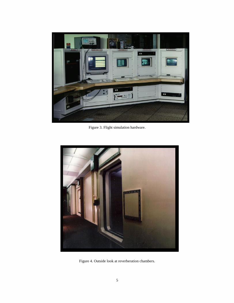
The flight simulator hardware is based on a twenty-slot VME backplane, Figure 3. The system

consists of three Motorola 68040 based real time controllers, five digital to analog converters (DAC), one analog to digital converter (ADC), and one MIL-STD-1553 interface board. The five DAC’s and one ADC link the simulator to the analog electro/optic converter, and the MIL-STD-1553 board links to the digital electro/optic converter. Even with five DAC’s and one ADC, only one set of input/output lines can be supported. Consequently, the analog electro/optic converter performs a fan out function so that all four of the flight control computer’s processors receive the same inputs.

The electromagnetic test chamber shown in Figure 2 is a 13 x 23 x 9½ foot mode-stirred

reverberation chamber located in the High Intensity Radiated Fields Laboratory at LaRC [15]. Figure 4 shows a picture of the outside of the test chambers. These are enclosed steel rooms that have been validated for shielding effectiveness to 120 dB to ensure that no radiation leaks outside of the chamber. The door is pneumatic in nature and has a seal that expands after the door is shut to ensure proper shielding. In essence, this is like a large microwave oven that provides a near homogeneous radiation environment. Using this type of test chamber enables the flight control computer to be exposed equally from all angles, so that the angle of incidence for maximum susceptibility does not need to be found or assumed.

Figure 2. Flight control computer placed in reverberation chamber to collect data.

5

Figure 3. Flight simulation hardware.

Figure 4. Outside look at reverberation chambers.

6

For the open-loop experiments, two special conditions were implemented. First, the flight simulation software was removed and the flight simulator was reprogrammed with a special calibration procedure. This procedure sent pre-selected reference voltages to each processor in the flight control computer in order to measure the noise level on the analog lines. The received voltages were then stored for comparison to the sent reference voltage.

The second condition was that, with the above calibration procedure in place, the passive filters

were selectively removed to introduce electromagnetic energy in the cables. This allowed the long electrical signal lines to couple electromagnetic energy into the flight control computer. These filters are extremely efficient at keeping the flight control computer radiation tight, so by removing specific combinations of filters the flight control computer processor could be weakened to the radiated energy. These combinations are shown in Table 1. The ninth cable cannot be removed because this supplies power to the flight control computer.

Table 1. Passive Filters Selectively Removed for the Open-Loop Experiments Filters Removed Test Objective

1, 5 Weaken Processor 1

2, 6 Weaken Processor 2

3, 7 Weaken Processor 3

4, 8 Weaken Processor 4

1, 2, 3, 4 Upper connector matrix cross-talk effects

5, 6, 7, 8 Lower connector matrix cross-talk effects

The maximum and minimum voltages were calculated for each analog signal line and three critical points were defined: fifty percent of the maximum voltage, the zero point, and fifty percent of the minimum voltage, as shown in Table 2. Appendix A lists the actual reference voltages sent for each signal.

Table 2. Pre-Selected Reference Voltages Sent to the Flight Control Computer

Voltage Level +15 to –15 v +10 to 0 volts

50% of Max +7.5 +5

Zero 0 0

50% of Min -7.5 0 One hundred percent of the maximum and minimum values were never sent to the controller

because with the added energy from the electromagnetic fields, the cumulative effect could have exceeded the hardware’s specification and resulted in component damage. Table 3 shows the effect the passive filters have on the system. The values shown reflect the overall maximum and minimum voltages

7

collected during testing. When the passive filters remain on the cables, there may be a nominal amount of radiation that enters the system that could minimally affect the voltage values received, see Table 3a. However, when the passive filters are removed, there is a change in the data collected, see Table 3b, which could have led to equipment damage if the maximum voltage threshold had been exceeded.

Table 3(a). Voltage Values Collected with Passive Filter On

Sent Received Min Max -4.995 -5.034 -4.832 0.000 -0.063 0.182 4.990 4.958 5.153

Table 3(b). Voltage Values Collected with Passive Filter Off

Sent Received Min Max -4.995 -5.230 -0.859 0.000 -0.216 4.113 4.990 4.790 9.035

Figure 5 shows the flowchart for the automated calibration procedure. For a single run of the

program 525,000 voltages were collected. The program was run for each of the six filter combinations listed in Table 1 which nets a total of 3,150,000 data points per test.

Figure 5. Flowchart for specialized calibration procedure.

Once the nominal characterization data was collected, a test plan was developed to obtain data

from the flight control computer on the effects of radiated fields within the test chamber. Testing started

Set all lines to-50% voltage.

Collect 1,000 samplesfor each of the four

processors.

Third timethrough? No

Yes

Store 3,000 samples x35 lines x 5 voltage

values as a file.

Increment tonext voltage

level.

8

at 250 MHz and was incremented by 100 MHz steps until reaching a maximum of 950 MHz. Field strengths were incremented as shown in Table 4.

The procedure followed for testing was to start at the lowest frequency and continue increasing the field strength to the highest level in Table 4, each time collecting the 3,150,000 data points described previously. However, tests were not conducted at all frequency/field strength pairs. Entries in the test matrix of Figure 4 indicate the test was halted if a large number of observed voltages violated a predetermined threshold, typically one percent above normal system drift. This test procedure was used for the indicated test configurations referenced in Table 1.

Table 4. Open-Loop Experiment Test Matrix Field Strength (v/m)

50 100 150 200 300 400 450 500 550 600 250 X X X X 350 X X X X 450 X X X X X X X X 550 X X X X X X X X 650 X X X X X X X X 750 X X X X X X X X 850 X X X X X X X X

Frequency (MHz)

950 X X X X X X X X Data were stored in an ASCII file with five columns, one for the reference voltage sent and one

column for voltages collected at each of the four processors. Each data file included three thousand samples, one thousand samples for each of the three reference voltage groups. Figure 6 shows a partial data file collected. Due to the overwhelming amount of data collected, one of the first tasks was to develop a data management scheme. This scheme involved standardizing file conventions such as file naming, data format, and data variables collected from the tests. It also involved storing the data to a medium that was accessible to all users and creating web pages that listed the unique test parameters and the directory locations of all files.

3 Statistical Modeling of Open-Loop Experiments In order to examine the open-loop test data, a reduced representation was required. The first

effort involved plotting the data for all frequency/field strength combinations. Figure 7 shows an arbitrarily chosen plot of the test data for “spl”, left spoiler in degree. Each subplot represents a different set of data for the signal. The columns depict the reference voltage sent while the rows are the field strengths. The first column of subplots represents fifty percent of the minimum voltage sent, the second column represents the zero point, and the third column represents fifty percent of the maximum voltage. For comparison sake, all column axes have the same values.

The first row shows the three reference voltage levels at one field strength. Each subsequent row

shows an increasing field strength at the same reference voltage level as that above it. As the field strength increases, the plots flatten out and the data begins to spread over a broader voltage range. This trend appeared in all of the test data examined.

9

Next, distribution curves were fit to the data since the data had no well-defined shape. The distributions that were fit to the data include the Uniform, Normal, Weibull, Rayleigh, Beta, Gamma, Exponential, and Pareto distributions [16, 17]. The distributions fit to the data, along with their associated probability density functions, are shown in Table 5. Using the method of least squares, it was determined that the curve that best fit the data overall was produced by the Normal distribution and therefore from this point forward this work will concentrate on the Normal distribution. The equation used to define the Normal distribution, as shown in Table 5, has x as the voltage value, µ the mean of the data, and σ2 the variance of the data.

- 4 . 9 9 5 - 5 . 0 1 3 - 5 . 0 1 3 - 5 . 0 0 6 - 5 . 0 0 6- 4 . 9 9 5 - 4 . 9 9 2 - 5 . 0 1 3 - 5 . 0 2 0 - 4 . 9 9 9- 4 . 9 9 5 - 4 . 9 8 5 - 5 . 0 2 7 - 5 . 0 0 6 - 4 . 9 9 9- 4 . 9 9 5 - 4 . 9 9 9 - 5 . 0 1 3 - 5 . 0 0 6 - 5 . 0 0 6- 4 . 9 9 5 - 4 . 9 6 5 - 5 . 0 1 3 - 4 . 9 9 9 - 4 . 9 9 2- 4 . 9 9 5 - 4 . 9 6 5 - 5 . 0 1 3 - 4 . 9 9 9 - 5 . 0 1 3- 4 . 9 9 5 - 4 . 9 6 5 - 5 . 0 1 3 - 5 . 0 0 6 - 4 . 9 9 9- 4 . 9 9 5 - 4 . 9 5 1 - 5 . 0 2 0 - 5 . 0 2 0 - 4 . 9 9 9- 4 . 9 9 5 - 4 . 9 5 1 - 5 . 0 1 3 - 5 . 0 1 3 - 4 . 9 9 2- 4 . 9 9 5 - 4 . 9 9 2 - 5 . 0 2 7 - 4 . 9 9 9 - 4 . 9 9 9- 4 . 9 9 5 - 5 . 0 1 3 - 5 . 0 1 3 - 5 . 0 0 6 - 5 . 0 1 3- 4 . 9 9 5 - 5 . 0 1 3 - 5 . 0 1 3 - 5 . 0 0 6 - 5 . 0 0 6- 4 . 9 9 5 - 4 . 9 9 2 - 5 . 0 1 3 - 5 . 0 1 3 - 4 . 9 9 9- 4 . 9 9 5 - 4 . 9 4 4 - 5 . 0 1 3 - 4 . 9 9 9 - 4 . 9 9 9- 4 . 9 9 5 - 4 . 9 7 1 - 5 . 0 3 4 - 5 . 0 1 3 - 4 . 9 9 9- 4 . 9 9 5 - 4 . 9 7 1 - 5 . 0 1 3 - 5 . 0 0 6 - 4 . 9 9 9- 4 . 9 9 5 - 4 . 9 5 8 - 5 . 0 0 6 - 4 . 9 9 9 - 5 . 0 0 6- 4 . 9 9 5 - 4 . 9 9 2 - 5 . 0 1 3 - 5 . 0 1 3 - 4 . 9 9 9- 4 . 9 9 5 - 4 . 9 9 9 - 5 . 0 1 3 - 5 . 0 1 3 - 4 . 9 9 9- 4 . 9 9 5 - 4 . 9 7 8 - 5 . 0 2 0 - 5 . 0 1 3 - 4 . 9 9 9- 4 . 9 9 5 - 4 . 9 7 1 - 5 . 0 1 3 - 5 . 0 1 3 - 5 . 0 0 6- 4 . 9 9 5 - 4 . 9 7 1 - 5 . 0 0 6 - 5 . 0 1 3 - 4 . 9 9 9- 4 . 9 9 5 - 4 . 9 6 5 - 5 . 0 1 3 - 5 . 0 0 6 - 5 . 0 0 6- 4 . 9 9 5 - 4 . 9 9 9 - 5 . 0 2 0 - 5 . 0 2 0 - 4 . 9 9 9- 4 . 9 9 5 - 4 . 9 6 5 - 4 . 9 9 9 - 5 . 0 0 6 - 5 . 0 0 6- 4 . 9 9 5 - 4 . 9 9 2 - 5 . 0 2 7 - 5 . 0 0 6 - 5 . 0 0 6- 4 . 9 9 5 - 4 . 9 9 9 - 5 . 0 1 3 - 5 . 0 0 6 - 5 . 0 2 0- 4 . 9 9 5 - 5 . 0 1 3 - 5 . 0 1 3 - 5 . 0 0 6 - 4 . 9 9 9- 4 . 9 9 5 - 5 . 0 1 3 - 5 . 0 1 3 - 5 . 0 0 6 - 4 . 9 9 9- 4 . 9 9 5 - 4 . 9 9 9 - 5 . 0 1 3 - 4 . 9 9 9 - 5 . 0 0 6- 4 . 9 9 5 - 4 . 9 9 2 - 5 . 0 2 0 - 5 . 0 0 6 - 4 . 9 9 9- 4 . 9 9 5 - 4 . 9 7 1 - 5 . 0 1 3 - 4 . 9 9 9 - 5 . 0 3 4- 4 . 9 9 5 - 4 . 9 7 1 - 5 . 0 1 3 - 4 . 9 9 9 - 5 . 0 0 6- 4 . 9 9 5 - 4 . 9 9 9 - 5 . 0 1 3 - 4 . 9 9 2 - 5 . 0 0 6- 4 . 9 9 5 - 5 . 0 0 6 - 5 . 0 1 3 - 5 . 0 1 3 - 5 . 0 0 6- 4 . 9 9 5 - 5 . 0 1 3 - 5 . 0 1 3 - 5 . 0 1 3 - 5 . 0 0 6- 4 . 9 9 5 - 4 . 9 9 9 - 5 . 0 2 0 - 4 . 9 9 9 - 5 . 0 0 6- 4 . 9 9 5 - 5 . 0 0 6 - 5 . 0 1 3 - 4 . 9 9 9 - 4 . 9 9 9- 4 . 9 9 5 - 5 . 0 3 4 - 5 . 0 2 0 - 5 . 0 0 6 - 5 . 0 0 6- 4 . 9 9 5 - 4 . 9 9 9 - 5 . 0 1 3 - 5 . 0 1 3 - 5 . 0 2 0- 4 . 9 9 5 - 4 . 9 7 1 - 5 . 0 1 3 - 5 . 0 1 3 - 4 . 9 9 9- 4 . 9 9 5 - 4 . 9 7 8 - 5 . 0 3 4 - 5 . 0 0 6 - 5 . 0 0 6- 4 . 9 9 5 - 4 . 9 9 9 - 5 . 0 2 0 - 5 . 0 1 3 - 4 . 9 9 9- 4 . 9 9 5 - 4 . 9 9 9 - 5 . 0 1 3 - 5 . 0 0 6 - 5 . 0 0 6- 4 . 9 9 5 - 4 . 9 7 8 - 5 . 0 1 3 - 5 . 0 0 6 - 5 . 0 2 0- 4 . 9 9 5 - 4 . 9 4 4 - 5 . 0 2 0 - 5 . 0 0 6 - 4 . 9 9 9- 4 . 9 9 5 - 4 . 9 1 6 - 5 . 0 3 4 - 5 . 0 1 3 - 5 . 0 0 6- 4 . 9 9 5 - 4 . 9 3 7 - 5 . 0 2 7 - 5 . 0 1 3 - 4 . 9 9 2- 4 . 9 9 5 - 4 . 9 5 8 - 5 . 0 1 3 - 5 . 0 0 6 - 5 . 0 0 6- 4 . 9 9 5 - 4 . 9 7 8 - 5 . 0 2 0 - 5 . 0 0 6 - 4 . 9 9 2- 4 . 9 9 5 - 5 . 0 0 6 - 5 . 0 1 3 - 4 . 9 9 9 - 4 . 9 8 5- 4 . 9 9 5 - 4 . 9 5 1 - 5 . 0 1 3 - 4 . 9 9 2 - 4 . 9 9 9- 4 . 9 9 5 - 4 . 9 6 5 - 5 . 0 1 3 - 5 . 0 0 6 - 5 . 0 0 6- 4 . 9 9 5 - 4 . 9 8 5 - 5 . 0 1 3 - 5 . 0 1 3 - 5 . 0 1 3- 4 . 9 9 5 - 4 . 9 5 8 - 5 . 0 1 3 - 4 . 9 9 9 - 4 . 9 9 9- 4 . 9 9 5 - 4 . 9 6 5 - 5 . 0 1 3 - 5 . 0 1 3 - 4 . 9 9 2- 4 . 9 9 5 - 4 . 9 7 8 - 5 . 0 1 3 - 5 . 0 1 3 - 5 . 0 0 6- 4 . 9 9 5 - 4 . 9 8 5 - 5 . 0 2 0 - 5 . 0 0 6 - 5 . 0 0 6- 4 . 9 9 5 - 4 . 9 9 9 - 5 . 0 0 6 - 4 . 9 9 9 - 4 . 9 9 9

noflt1/550cw/100vm/sr4phidts.datVoltage Sent Received P1 Received P2 Received P3 Received P4

Figure 6. Partial open-loop experiment data file collected.

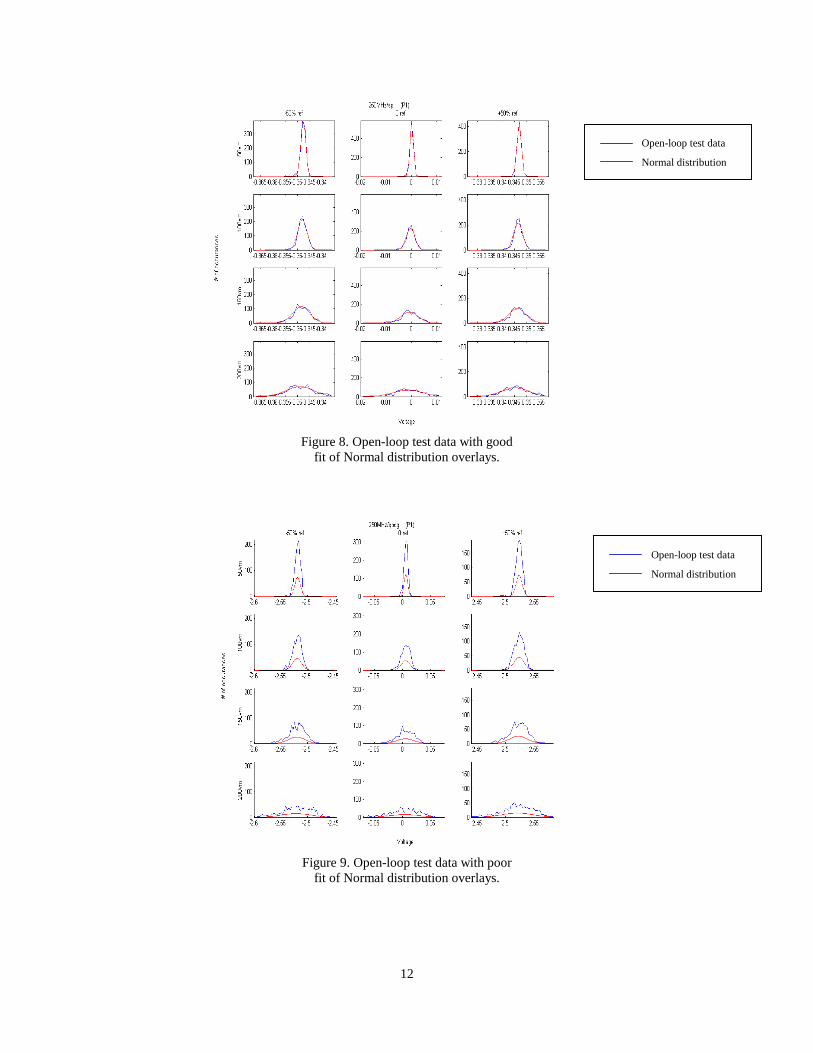
Figure 8 shows the same data as Figure 7 with the Normal distribution curve overlaying the data

values. For this particular signal, the Normal distribution has a good fit. There were some signals in which the Normal distribution did not fit the data as well, see Figure 9. However, the Normal distribution was the best fit of the distributions tried. Upon studying the patterns of the data with the distribution overlay curves, it was obvious that a scaling factor was needed to model some of the data. The model with scaling factor that will be used is defined as:

10

( )

σπβα= σ

µ−−22

2x

e2

1)x(f (1)

where α = maximum number of occurrences from the collected voltages β = maximum value previously calculated for the Normal distribution x = collected voltages µ = mean of collected voltages σ = standard deviation of collected voltages

The scaling factor that was used came from multiplying the Normal distribution by the maximum number of occurrences from the collected voltages divided by the maximum value calculated for the Normal distribution. Figure 10 shows a plot with the original test data, the Normal distribution curve, and the Normal distribution curve with a scaling factor incorporated. The curve with the scaling factor fits the data and will be used in further analysis. At this point the first goal of the research has been met which was to develop and validate a mathematical model of the electromagnetic fields coupling into the equipment.

Figure 7.Subplot of open-loop test data.

11

Table 5. Distributions Used to Fit the Open-Loop Experiment Data Distribution Probability density function Uniform ( )

elsewhere,0

;bxa,ab

1xf <<

−=

Normal

( )( )

0,x

;x,e2

1xf

22

2x

>σ∞<<∞−

∞<<∞−σπ

= σ

µ−−

Weibull

( )

elsewhere,0

0,;0x,exxf

x

1 >θα>θ

α=

α

θ−

−αα

Rayleigh

( ) 0x,ex

xf22

2x

2>

σ=

σ

−

Beta ( ) ( )( ) ( ) ( )

elsewhere,0

0,;1x0,x1xxf 11 >βα<<−βΓαΓβ+αΓ= −β−α

Gamma ( ) 0r,dxexr 0x1r >∫=Γ ∞ −−

Exponential

( )elsewhere,0

0,0x,e1

xf

x

>θ>λ

= λ−

Pareto ( )( )

∞<θ<∞<<+

θ=+θ

0,x0x1

xf1

12

Figure 8. Open-loop test data with good

fit of Normal distribution overlays.

Figure 9. Open-loop test data with poor

fit of Normal distribution overlays.

Open-loop test data

Normal distribution

Open-loop test data

Normal distribution

13

Figure 10. Open-loop test data with Normal distribution

and scaling factor overlays.

The focus will now be on the second goal of the research which is to use the model to

extrapolate/predict measurements that are outside of the given data. The first effort of this statistical analysis involved finding the least square error using the equation:

( )[ ]n

1i

2ii xpyL

=−∑= (2)

where y is the test data and p(x) is the calculated Normal distribution value [16]. The method of least squares chooses solutions with coefficients that minimize the sum of the

squares of the vertical distances from the data points, which are presumed to be polynomial [16]. The best-fit polynomial is the one with coefficients that minimize the function L. Figure 11 shows a representative plot where the least square error was calculated for each field strength and reference voltage for one particular frequency and signal. The text in the individual subplots indicates which set of parameters best fit the curve. Some data have better least square error estimates than others do, while the one that is represented in the subplots is the best fit (lowest value) of the least square error combinations tried.

There were numerous least square error parameters to look at. Table 6 describes the different

means and variances that were calculated and compared to find the lowest value of the least square error. The 'Lxy' number displayed in the subplots represents the combination of parameters used to find the least square error. The 'x' (which is 1, 2, or3) indicates which reference voltage was used while 'y' (which is 0 through 15) describes the mean and variance combination used to test different least square errors.

Open-loop test data

Normal distribution

Normal distribution with scaling factor

14

Figure 11. Open-loop test data with least square error overlays.

Table 6. Mean and Variance Combinations Used to Determine the Least Square Error Value y Mean Variance 0 mean of matrix variance of matrix 1 mean of matrix sample variance 2 mean of matrix variance of non-repeated matrix 3 midpoint of matrix variance of matrix 4 midpoint of matrix sample variance 5 midpoint of matrix variance of non-repeated matrix 6 midpoint of sorted, non-repeated matrix variance of matrix 7 midpoint of sorted, non-repeated matrix sample variance 8 midpoint of sorted, non-repeated matrix variance of non-repeated matrix 9 mean of non-repeated matrix variance of matrix 10 mean of non-repeated matrix sample variance 11 mean of non-repeated matrix variance of non-repeated matrix 12 voltage with most occurrences variance of matrix 13 voltage with most occurrences sample variance 14 voltage with most occurrences variance of non-repeated matrix 15 *amp factor maximum voltage variance of non-repeated values Once the least square error with the lowest value was determined, the mean and variance that

supported that least square error were saved to different four-dimensional matrices (field strength x reference voltage x signal x frequency). Using these new parameters, the values for all of the field strengths for one frequency and signal were plotted to graphs. Figure 12 shows a typical graph of the new parameters. The top subplot represents the variances collected using the least square error method. Since

Raw data

Least square error

15

all of the reference voltages have similar variances, this is a good indicator that the analysis was done properly. The bottom subplot represents the means that were collected. This particular signal had minimal fluctuation in the means collected. All of the graphs produced were then studied to determine what direction to take for further analysis.

Figure 12. New mean and variance parameters generated

from the least square error value. The means found using the least square error method varied only slightly for most of the signals,

so the first focus was on how to extrapolate the variance. This effort involved extrapolating data by hand from the new parameters found from the least square error method. This technique produced eight signals as having the most variable movement. This hand plotting technique was tedious and became unwieldy after a few attempts. The next step was to use an automated computer tool to extrapolate the values to the predetermined level of 1000v/m. The values that were extrapolated depended on the frequency that was being examined, as shown in Table 7.

The basic fitting interface allows the data to be fit using an interpolant or a polynomial (up to

degree 10). It permitted multiple fits to be plotted simultaneously so that comparison for the given data set could be made. It also permitted examination of the numerical residual of a fit, to evaluate the fit, and to save the evaluated results to a Matlab variable. The results of the numerous basic fitting interface computations were usually cubic in nature, but there were several that were linear or quadratic.

The best fit was determined by examining the numeric value of the norm of the residuals and the residual plots. The fit residuals are defined as the difference between the ordinate data point and the resulting fit for each abscissa data point. The norm of the residuals is a measure of the goodness of fit, where a smaller value indicates a better fit than a larger value. During this analysis, several of the fits had

16

negative values when extrapolated and it was necessary to return to the basic fitting interface and consider a different fit. Once the best fit was determined, the fit was extrapolated using the values from Table 7.

Table 7. Field Strengths Extrapolated at Each Frequency

Frequency (MHz) Extrapolated Field Strengths (v/m) 250 300, 400, 500, 600, 700, 800, 900, 1000 350 300, 400, 500, 600, 700, 800, 900, 1000 450 650, 700, 750, 800, 850, 900, 950, 1000 550 650, 700, 750, 800, 850, 900, 950, 1000 650 650, 700, 750, 800, 850, 900, 950, 1000 750 650, 700, 750, 800, 850, 900, 950, 1000 850 650, 700, 750, 800, 850, 900, 950, 1000 950 650, 700, 750, 800, 850, 900, 950, 1000

Figure 13 shows a typical result from the basic fitting interface tool. The top subplot shows the

test data, a quadratic fit, and a cubic fit. The two fits are very close and must have another step introduced in order to find the best fit. Using the basic fitting interface tool the analysis can be expanded to include the residuals, this is represented in the bottom subplot of Figure 13. This subplot shows a plot of the residuals with the value of the norm of the residuals. As stated before, the lower the value of the norm of the residual, the better the fit. Therefore, in this case, because the norm of the residual for the cubic fit was lower than that of the quadratic fit, the cubic fit was used to extrapolate the values of the variance.

Figure 13. Plot generated by Matlab's basic fitting interface.

17

Figure 14 shows the extrapolated values in the top subplot. The '+' marks show the previously

calculated variances using the least square error method, while the '◊' marks show the values that were extrapolated using the basic fitting interface tool. These values were calculated with the tool and then stored.

Figure 14. Plot of extrapolated variances using

Matlab's basic fitting interface.

Figure 15 shows a plot with the mean and median of the test data plotted. The upper dotted line in the figure represents the median while the lower dotted line is the mean. In most cases, the median seemed to represent the test data better and was used for the mean value in further analyses.

Once the variances and means had been obtained, the developed mathematical model could be

used to plot the Normal distribution using these extrapolated values. Figure 16 shows subplots of the scaled Normal distribution using the extrapolated values for the mean and variance. These plots follow the same trend that was referred to before, as the field strength increases the data becomes flatter and spreads out over a broader voltage range.

After studying the data and applying numerous statistical tests, including Chi square, student t

distributions, and confidence intervals, it has been determined that the field strength can be increased up to 1000 v/m without damaging the equipment. Therefore, at this point the initial objectives of this research have been accomplished.

18

Figure 15. Mean/median computed using

Matlab's data statistics tool.

19

Figure 16. Normal distribution using the

extrapolated variance and mean

20

4 Conclusions The preliminary objectives of this research have been accomplished. A mathematical model of

the electromagnetic radiation coupling into the flight control computer has been developed and validated. Thousands of representations of the open-loop test data were plotted for comparison. A trend in

the data was discovered that warranted fitting distribution curves to the data. Because the data had no well-defined shape, selected distribution curves were fit to the data and the Normal distribution was found to have the best overall fit. It was determined that the Normal distribution needed a scaling factor. Using the experiment data, a scaled normal probability density function was developed and validated. Using the scaled Normal distribution as the standard, the least square error was then calculated. The mean and variance that supported the least square error with the lowest value were plotted for all field strengths for one frequency and signal. These plots were used to extrapolate the variances and the means.

Using the extrapolated values for the variances and means, the developed mathematical model

was used to plot the Normal distribution for the field strengths that had been extrapolated. These plots followed the same trend as the test data: as the field strength increases, the amplitude of the voltage flattens and the voltage range covers a broader region. Examining the extrapolated plots led to the conclusion that more tests can be performed and the field strength can be increased to the predetermined field strength of 1000 v/m without damaging the equipment.

21

Appendix A Reference voltages sent for each signal

Signal Min Zero Max cas -4.7800 0 4.7750 delac -5.0000 0 5.0000 delec -5.0000 0 5.0000 delrc -5.0000 0 5.0000 deltc -5.0000 0 5.0000 epr -4.6880 0 4.6830 eta -4.3850 0 4.3800 gamma -2.8810 0 2.8760 gse -2.5000 0 2.4980 hddot -2.5000 0 2.4980 hdot -5.0000 0 4.9950 phidg -5.0000 0 4.9950 phidt -4.9950 0 4.9900 psidt -4.4970 0 4.4920 qbdg -2.5000 0 2.4980 ralt -4.9900 0 0 rbdg -2.4950 0 2.4930 spl -2.9100 0 2.9050 spr -2.9100 0 2.9050 tas -4.7800 0 4.7750 tbax -0.9910 0 0.9890 thrtrm -5.0000 0 4.9950 tk -4.4970 0 4.4920 vele -2.8710 0 2.8660 veln -1.2500 0 1.2490 vgs -2.5000 0 2.4980 vgsdt -5.0000 0 4.9950 ycg -1.2490 0 1.2480

22

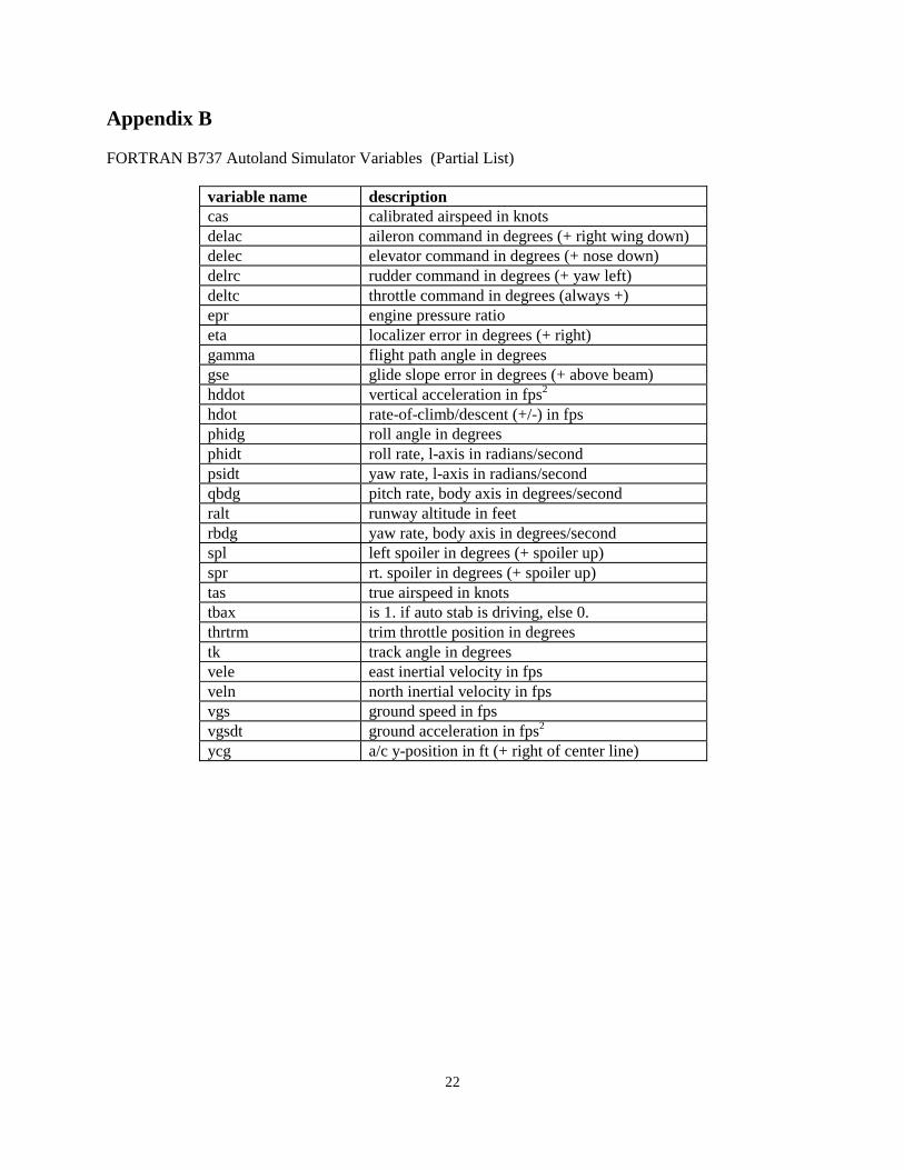
Appendix B FORTRAN B737 Autoland Simulator Variables (Partial List)

variable name description cas calibrated airspeed in knots delac aileron command in degrees (+ right wing down) delec elevator command in degrees (+ nose down) delrc rudder command in degrees (+ yaw left) deltc throttle command in degrees (always +) epr engine pressure ratio eta localizer error in degrees (+ right) gamma flight path angle in degrees gse glide slope error in degrees (+ above beam) hddot vertical acceleration in fps2 hdot rate-of-climb/descent (+/-) in fps phidg roll angle in degrees phidt roll rate, l-axis in radians/second psidt yaw rate, l-axis in radians/second qbdg pitch rate, body axis in degrees/second ralt runway altitude in feet rbdg yaw rate, body axis in degrees/second spl left spoiler in degrees (+ spoiler up) spr rt. spoiler in degrees (+ spoiler up) tas true airspeed in knots tbax is 1. if auto stab is driving, else 0. thrtrm trim throttle position in degrees tk track angle in degrees vele east inertial velocity in fps veln north inertial velocity in fps vgs ground speed in fps vgsdt ground acceleration in fps2 ycg a/c y-position in ft (+ right of center line)

23

References 1. NASA Facts, Dryden Flight Research Center: "F-8 Digital Fly-By-Wire Aircraft".

http://www.dfrc.nasa.gov/PAO/PAIS/HTML/FS-024-DFRC.html Accessed August 28, 2002.

2. Dryden Flight Research Center: "Digital Fly-By-Wire".

http://www.dfrc.nasa.gov/Projects/f8/home.html Accessed August 28, 2002. 3. Smith, Jr., Albert A.: Coupling of External Electromagnetic Fields to Transmission

Lines. Second ed., Interference Control Technologies, Inc., 1989. 4. Fuller, Gerald: "Understanding HIRF". Avionics Communications Inc., 1995. 5. Belcastro, Celeste M.: Detecting Upset in Fault Tolerant Control Computers Using Data

Fusion Techniques. Ph.D. Thesis, Drexel University, December 1994. 6. Belcastro, Celeste M.: Digital System Upset - The Effects of Simulated Lightning-Induced

Transients on a General Purpose Microprocessor. NASA TM-84652, 1983. 7. Belcastro, Celeste M.: Data and Results of a Laboratory Investigation of Microprocessor

Upset Caused by Simulated Lightning-Induced Analog Transients. NASA TM-85821, 1984.

8. Clough, Bruce T.: Microwave Induced Upset on a Digital Flight Control Computer.

Digital Avionics Systems Conference, Fort Worth, TX, 1993. 9. Davidoff, A.; Schmid, M.; Trapp, R.; and Masson, G.: Monitors for Upset Detection in

Computer Systems. Proceedings of the International Aerospace and Ground Conference on Lightning and Static Electricity, Fort Worth, TX, 1983.

10. Masson, G. M.; and Glaser, R. E.: Intermittent/Transient Faults in Digital Systems.

NASA CR-169022, 1982. 11. Hanson, R. J.: Subsystem EMP Strength Verification Methods: Upset Detection and

Evaluation for Military Subsystems. WL-TR-89-19, August 1989. 12. FAA Advisory Circular 20-136: Protection of Aircraft Electrical/Electronic Systems

against the Indirect Effects of Lightning. March 1990. 13. Smith, Laura J.; and Koppen, Daniel M.: Determination of Upper Destructive Limit for

HIRF Experiments on a Fault Tolerant Flight Control Computer. AIAA/IEEE 17th DASC Proceedings, October 1998.

14. Koppen, Daniel M.: Open-Loop HIRF Experiments Performed on a Fault Tolerant Flight

Control Computer. AIAA/IEEE 16th DASC Proceedings, October 1997. 15. Williams, Reuben A.: The NASA High-Intensity Radiated Fields Laboratory. AIAA/IEEE

16th DASC Proceedings, October 1997.

24

16. Larsen, Richard J.; and Marx, Morris L.: An Introduction to Mathematical Statistics and

Its Applications. Second ed., Prentice-Hall, 1986. 17. Canavos, George C.: Applied Probability and Statistical Methods. Little, Brown and

Company Limited, 1984.

REPORT DOCUMENTATION PAGE Form ApprovedOMB No. 0704-0188

2. REPORT TYPE

Technical Memorandum 4. TITLE AND SUBTITLE

A Numerical Simulation and Statistical Modeling of High Intensity Radiated Fields Experiment Data

5a. CONTRACT NUMBER

6. AUTHOR(S)

Smith, Laura J.

7. PERFORMING ORGANIZATION NAME(S) AND ADDRESS(ES)

NASA Langley Research CenterHampton, VA 23681-2199

9. SPONSORING/MONITORING AGENCY NAME(S) AND ADDRESS(ES)

National Aeronautics and Space AdministrationWashington, DC 20546-0001

8. PERFORMING ORGANIZATION REPORT NUMBER

L-18356

10. SPONSOR/MONITOR'S ACRONYM(S)

NASA

13. SUPPLEMENTARY NOTESAn electronic version can be found at http://techreports.larc.nasa.gov/ltrs/ or http://ntrs.nasa.gov

12. DISTRIBUTION/AVAILABILITY STATEMENTUnclassified - UnlimitedSubject Category 66Availability: NASA CASI (301) 621-0390 Distribution: Standard

19a. NAME OF RESPONSIBLE PERSON

STI Help Desk (email: help@sti.nasa.gov)

14. ABSTRACT

Tests are conducted on a quad-redundant fault tolerant flight control computer to establish upset characteristics of an avionics system in an electromagnetic field. A numerical simulation and statistical model are described in this work to analyze the open loop experiment data collected in the reverberation chamber at NASA LaRC as a part of an effort to examine the effects of electromagnetic interference on fly-by-wire aircraft control systems. By comparing thousands of simulation and model outputs, the models that best describe the data are first identified and then a systematic statistical analysis is performed on the data. All of these efforts are combined which culminate in an extrapolation of values that are in turn used to support previous efforts used in evaluating the data.

15. SUBJECT TERMS

HIRF; High Intensity Radiated Fields; Electromagnetics; Open-Loop Testing; Statistical Analysis

18. NUMBER OF PAGES

29

19b. TELEPHONE NUMBER (Include area code)

(301) 621-0390

a. REPORT

U

c. THIS PAGE

U

b. ABSTRACT

U

17. LIMITATION OF ABSTRACT

UU

Prescribed by ANSI Std. Z39.18Standard Form 298 (Rev. 8-98)

3. DATES COVERED (From - To)

5b. GRANT NUMBER

5c. PROGRAM ELEMENT NUMBER

5d. PROJECT NUMBER

5e. TASK NUMBER

5f. WORK UNIT NUMBER

23-728-30-10

11. SPONSOR/MONITOR'S REPORT NUMBER(S)

NASA/TM-2004-213005

16. SECURITY CLASSIFICATION OF:

The public reporting burden for this collection of information is estimated to average 1 hour per response, including the time for reviewing instructions, searching existing data sources, gathering and maintaining the data needed, and completing and reviewing the collection of information. Send comments regarding this burden estimate or any other aspect of this collection of information, including suggestions for reducing this burden, to Department of Defense, Washington Headquarters Services, Directorate for Information Operations and Reports (0704-0188), 1215 Jefferson Davis Highway, Suite 1204, Arlington, VA 22202-4302. Respondents should be aware that notwithstanding any other provision of law, no person shall be subject to any penalty for failing to comply with a collection of information if it does not display a currently valid OMB control number.PLEASE DO NOT RETURN YOUR FORM TO THE ABOVE ADDRESS.

1. REPORT DATE (DD-MM-YYYY)

03 - 200401-