A NUMERICAL METHOD FOR THE PREDICTION OF HIGH-SPEED

BOUNDARY-LAYER TRANSITION USING LINEAR THEORY*

By Leslie M. Mack

Jet Propulsion Laboratory

SUMMARY

This paper describes a method of estimating the location of transitionin an arbitrary laminar boundary layer on the basis of linear stabilitytheory. After an examination of experimental evidence for the relationbetween linear stability theory and transition, a discussion is given ofthe three essential elements of a transition calculation: (1) the inter-action of the external disturbances with the boundary layer; (2) the growthof the disturbances in the .boundary layer; and (3) a transition criterion.A brief discussion is given of the computer program which carries out thesethree calculations. The program is first tested by calculating the effectof free-stream turbulence on .the transition of the Blasius boundary layer,,and is then applied to the problem of transition in a supersonic wind tunnelThe effects, of unit Reynolds number and Mach number on the transition of aninsulated flat-plate boundary.layer are calculated on the basis of experi-mental data on the intensity and spectrum of free-stream disturbances.Reasonable agreement with experiment is obtained in the Mach number rangefrom 2 to 4.5.

INTRODUCTION

One of the most difficult problems in theoretical aerodynamics is theprediction of transition from laminar to turbulent flow, a problem that is'especially severe for supersonic and hypersonic boundary layers. Examplesranging from high-velocity reentry vehicles to the wind-tunnel testing oftransonic airfoil sections can be put forward to illustrate the dramaticeffects on flow characteristics which result from differences in the loca-tion of transition. The search for some method of estimating whether theboundary layer will be laminar or turbulent for a particular external flowhas mostly focussed on empirical correlations of some type. These methodsare limited in scope and should be replaced by a more fundamental approachwhich involves the calculation of the development of the perturbed boundarylayer as it responds to its disturbance environment. The direct solutionof the three-dimensional time-dependent Navier-Stokes equation of compres-sible flow, which could be of great benefit, still lies in the future. Theuse of turbulence model equations is a promising approach although it re-mains to be demonstrated if enough of the complexity of the transition

*Research supported by NASA under Contract No. NAS 7 - 1 0 0 . ~ ~

101

https://ntrs.nasa.gov/search.jsp?R=19760002924 2018-06-24T04:10:58+00:00Z

process is retained in these time-averaged equations, which were primarilyintended for fully developed turbulent flow, to make them useful as a pre-diction technique. A third possibility is the use of linear stabilitytheory. This approach might at first appear to be of little value becauseof the evident nonlinearity of the final breakdown of laminar flow. However,it does have the considerable advantage that within the restrictions of line-arity and locally parallel flow one is dealing with solutions of the unsteadyNavier-Stokes equations. Furthermore, in many disturbance environments mostof the region preceding transition will involve a disturbance of small ampli-tude. In these cases, the process by which the dominant external disturb-ances form an organized wave structure in the_boundary layer, and the sub- .sequent growth of the internal boundary-layer disturbances both lie withinthe scope of a linear theory. Nonlinearity occurs only in a small regionimmediately preceding transition. Consequently, it should follow that atleast the change in the transition Reynolds number as the mean boundary layeror the disturbance environment changes can be calculated from linear theory.

In reference 1, a detailed investigation was carried out to determinewhether in a supersonic wind tunnel the change in the transition Reynoldsnumber of a flat-plate boundary layer with Mach number and surface coolingcan indeed be accounted for by linear theory. The results reported thereare sufficiently promising to encourage taking the next step, which is touse linear theory to make a quantitative estimate of the transition Reynoldsnumber. It is the purpose of this paper to describe a numerical method andcomputer program which combine information about the external disturbanceswith stability theory and a transition criterion to provide estimates oftransition location in a wide variety of cases. As examples, the effect ontransition of free-stream turbulence in low-speed flow, and of Mach numberand unit Reynolds number in a supersonic wind tunnel are given.

SYMBOLS

A disturbance amplitude

Aj free-stream disturbance amplitude

A0 initial disturbance amplitude

A amplitude transition criterion

c phase velocity, ou/a

E(oo) energy density of normalized power "spectrum

f frequency

102

dimensionless frequency, c»

L .' length scale

* /„ *2

integral length scale of turbulence*"

M . '.•:•• -.Mach number

p' . pressure fluctuation

Re .free-stream x-Reynolds number

RL Reynolds number based on LX . •

R.A displacement-thickness Reynolds number

u', v' velocity fluctuations • •

U . mean longitudinal velocity ;; •

U average source velocitys

x,y,z longitudinal, transverse and lateral coordinates

a complex wave number in x-direction, ot + ia.

P complex wave number in z-direction^ 3 + ip.

Y ratio of specific heats

(j, viscosity coefficient

V kinematic viscosity coefficient

T Reynolds stress ratioJx

(T ) Reynolds stress transition criterionR t -

i|t wave angle, tan"x(P /ot )

GO circular frequency

Superscripts:

( ) dimensional quantity

( )' .fluctuation quantity

103

( ) average quantity "

Subscripts:

t transition

i free-stream condition

o neutral-stability condition

LINEAR STABILITY THEORY AND TRANSITION

The idea of calculating boundary-layer transition by means of linearstability theory would be on much more solid ground if it were possible topoint to experimental evidence that there is indeed a direct quantitativerelation between linear instability and transition. Schubauer and Skramstad(ref. 2) demonstrated the correctness of the theory of Tollmien and Schlichtihgas a description of the behavior of small disturbances in the laminar boundarylayer preceding transition. They also showed that the location of transitioncould be changed by varying either the frequency or amplitude of an artificialdisturbance, but no quantitative results were given.

Apparently the only published" experiment that does offer quantitative'results in this regard is the one described in reference 3 by Jackson andHeckl. An axisymmetric model of circular cross section on which a Blasiusboundary layer formed was mounted in a wind tunnel of moderate turbulencelevel (0.2 - 0.4%). A loudspeaker was placed inside the model and the soundintroduced into the boundary layer through a circumferential slit located12 in. from the effective start of the boundary layer. Transition was fixed

-at &- point 15-in. downstream~of the slit for a range of frequencies by ad-justing the amplitude of the loudspeaker. The amplitude of the disturbancecreated in the boundary layer was monitored with a hot-wire anemometer locatedin the boundary layer above the slit. Transition was measured by a hot wirelocated at the downstream (15 in.) station and was judged to have "occurredwhen the disturbance spectrum changed to a turbulent form. Thus the endrather than the start of transition was being measured.

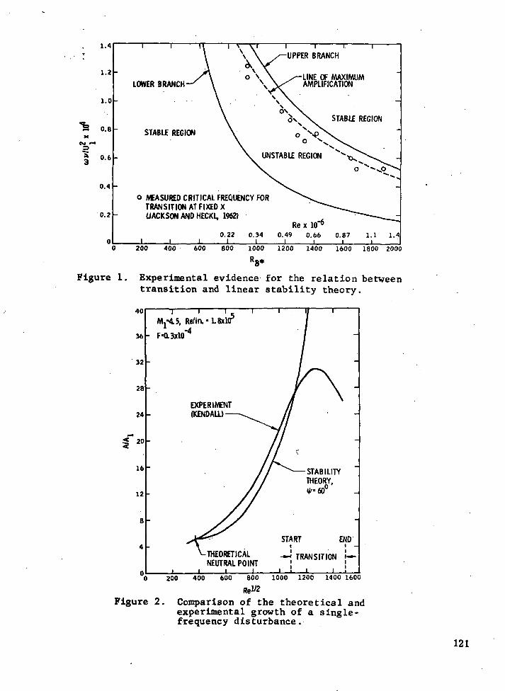
For a given free-stream velocity Uj (asterisks refer to dimensionalquantities) the frequency and amplitude were varied to find the frequencywhich resulted in transition at the downstream station with the smallestinitial amplitude. These frequencies are called the critical frequenciesand are shown on a typical stability diagram in figure 1 where the dimen-sionless frequency F = a^V^/U^* is plotted against Re, the free-streamx-Reynolds number, and RK*> the displacement-thickness Reynolds number.In, terms of linear stability theory, the experimental procedure was equiva-lent to finding the frequency with maximum total amplification at a givenReynolds number. Consequently, if the location of transition is determinedby the linear instability of the undisturbed laminar boundary layer, the

104

critical-frequency data points should lie along the theoretical line of maxi-mum amplification. Figure 1 shows that this condition is satisfied. Further-more, this close relation between transition and linear instability is notrestricted to what are commonly thought of as small disturbances. The transi-tion Reynolds numbers of figure 1 are between 0.3 X 106 and 1.2 x 106 whichwould correspond to free-stream turbulence levels of 0.4 to 1.67o if transitionwere caused solely by free-stream turbulence.

Finally, it must be remarked that stability and transition experimentswith artificially produced sound as the disturbance source are notoriouslydifficult to carry out, a situation already noted and discussed at some lengthin reference 2. It would be highly desirable to repeat the same type of ex-periment as in reference 3 with a different method of producing the artificialdisturbances .

With some experimental support available for the idea of using lineartheory for transition prediction, it only remains to decide on how to applythe theory. Any naturally occurring disturbance, will have its energy dis-tributed over a range of frequencies, and in the most general case its develop-ment in a boundary layer can only be calculated by considering the separatedevelopment of all frequencies with a significant portion of the total energy.However, amplification in a boundary layer is selective, and for small initialdisturbance levels the selectivity, or tuning, is sufficiently sharp so thatby the time transition is approached most of the disturbance energy is concen-trated in a narrow band about the most-amplified frequency. This phenomenonsuggests simplifying ,the application of stability theory by considering onlydisturbances of a single frequency. Such a procedure is possible because theamplification is linear and there is no transfer of energy from one frequencyto another. Therefore, transition will be predicted in this paper on thebasis of the single-frequency disturbance of maximum amplitude at each Reynoldsnumber. Since the amplitude of a disturbance at any Reynolds number dependson its initial amplitude as well as on the amplification it has undergone, itis necessary to consider the initial energy spectrum of the complete wide-banddisturbance to arrive at the single-frequency disturbance of maximum amplitude.

A comparison of the growth of the theoretical single-frequency disturb-ance of maximum amplitude at transition with the measured growth of the samefrequency component is shown in figure 2 for an insulated flat-plate boundarylayer in a supersonic wind tunnel at Mx = 4.5 and Re/in. = 1.8 x 10

5. Thedimensionless frequency of the two growth curves, F = 0.3 X 10~4, is the theo-retical frequency of the disturbance of maximum amplitude only if the initialenergy distribution of all single-frequency disturbances is identical to thepower spectrum of the free-stream disturbances as measured by Laufer (ref. 4).The experimental narrow-band disturbance growth is taken from Kendall's mea-surements (ref. 5) in the JPL 20-in. wind tunnel, the same.tunnel as used byLaufer. Because of the interaction of the irradiated sound from the turbulentboundary layers on the tunnel walls with the laminar boundary layer near theleading edge of the flat plate, there is. no experimentally discernible neutral-stability .point . The theoretical and experimental disturbance amplitudes arematched at the theoretical neutral point.

105

•'• The theoretical disturbance of maximum amplitude has a wave angle i|tequal to 60°, while the experimental narrow-band disturbance includes all Jwave angles. Unfortunately, the distribution of energy with respect towave angle in the experiment is unknown. Even so, the growths of the twodisturbances are seen to be closely related. By coincidence, the two growthcurves cross at almost exactly the start-of-trans ition Reynolds numbermeasured by Coles (ref. 6), also in the JPL 20-in. wind tunnel. The factthat transition occurs where the theoretical disturbance is growing rapidlymeans that a transition criterion based on amplitude has a good chance ofpredicting the start of transition provided only that the region of maximumgrowth-does vary, as assumed, with the mean-flow parameters" in "the same wayas the transition Reynolds number.

REQUIREMENTS OF TRANSITION CALCULATION

In addition to the calculation of.the velocity and temperature profilesof the mean.boundary layer, the transition calculation can be divided into,three distinct parts: (1) the interaction of the external disturbances whichlead to transition with the boundary layer to form the internal boundary-layerdisturbances of Tollmien-Schlichting type; (2) the growth of the internaldisturbances; and (3) a transition criterion, based on some property of thegrowing disturbances. In this section each of these three aspects will bediscussed separately starting with the second for reasons of clarity in theexposition.

Spatial Stability Theory v

The calculation of the disturbance growth in the boundary layer is the-element-which brings- in1 the -traditional" linear "stability'"theory r""A"detailed •account of compressible stability theory may be found in reference 7. Whatis required of the theory are the eigenvalues of the stability equations fora spatially growing disturbance. For the parallel-flow form of the' stabilityequations," a Fourier component of a typical three-dimensional fluctuation --quantity is given by

q'(x,y,z,t) = Q(y) exp [i(ox + 3y - cot) ] (1)

where q' is a small quantity; x,y,z are the longitudinal, transverse aridlateral coordinates'; Q(y) is a complex amplitude function; cu sis the realcircular frequency; and a and 3 are the complex wave numbers

(3 3 +r (2) .

j106

All quantities have been made dimensionless with respect to a length scaleL and a velocity scale V . The disturbance wave angle is

" . . ' • • * - tan~Mp lo t ) (3)r r . . .

and P /or is assumed equal to p /a . The phase velocity is ...

: - c =• ui/a (4)P r

and the imaginary part of cv is the amplification rate

(l/A)(dA/dx) = - a, (5)

The notation A has been introduced as the amplitude in equation (5) toemphasize that in the parallel-flow theory all flow variables grow atthe same rate and independently of y. The amplitude is given as a func-tion of Reynolds number by

Re

<YdRe)A(Re) Mo '- exp ( - ct. dRe ) (6)

The subscript o refers to the lower-branch neutral point, i.e., where thedisturbance has its minimum amplitude and first starts to amplify. Theinitial amplitude A0 is obviously of as much importance in determiningthe amplitude A as the amplification, and is the quantity that must beobtained from the external disturbance and an interaction relation.

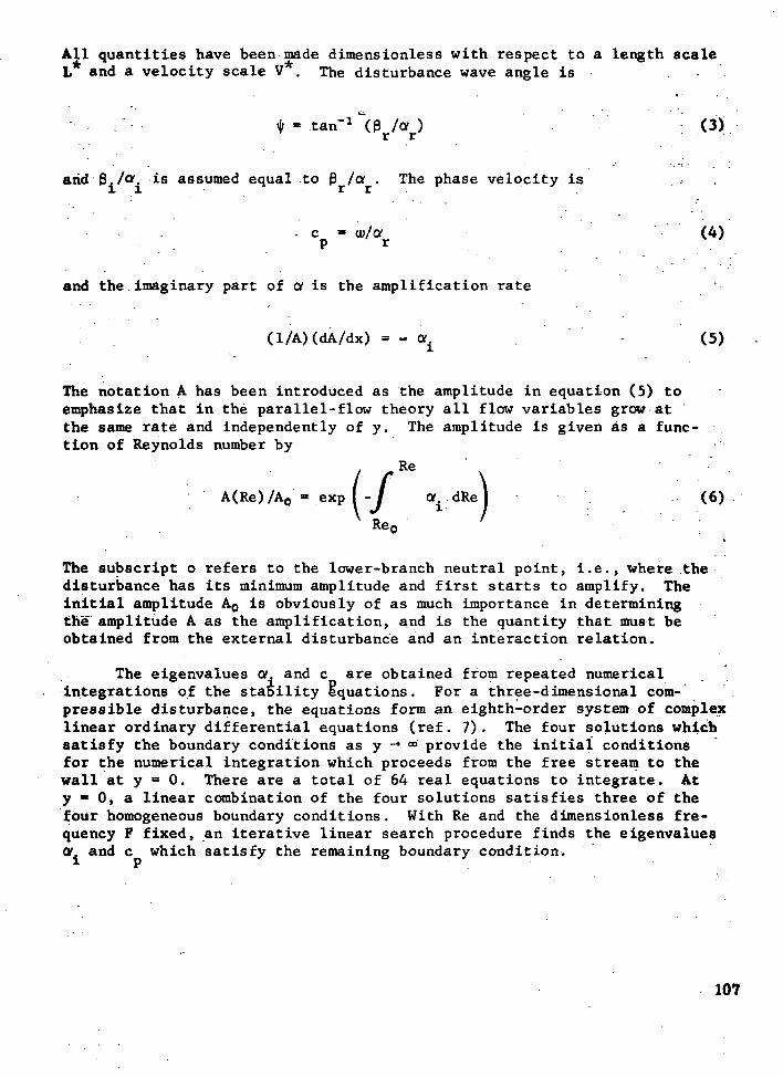
The eigenvalues a. and c are obtained from repeated numericalintegrations of the stability equations. For a three-dimensional com-pressible disturbance, the equations form an eighth-order system of complexlinear ordinary differential equations (ref. 7). The four solutions whichsatisfy the boundary conditions as y -» °° provide the initial conditionsfor the numerical integration which proceeds from the free stream to thewall at y = 0. There are a total of 64 real equations to integrate. Aty * 0, a linear combination of the four solutions satisfies three of thefour homogeneous boundary conditions. With Re and the dimensionless fre-quency F fixed, an iterative linear search procedure finds the eigenvaluesor and c which satisfy the remaining boundary condition.

107

Interaction of External Disturbances

, . Quantities computed directly from the linear stability theory suchas the minimum critical Reynolds number and amplification rate are inherentproperties of the mean boundary layer on the same basis as the displacementthickness or skin-friction coefficient. On the other hand, the transition.Reynolds number is not at all an inherent property as it depends not onlyon the instability of the boundary layer, but also on external disturbanceswhich interact with the boundary layer to form the internal disturbanceswhich lead"ultimately to transition. With no disturbances, transition cannot occur no matter how unstable the boundary layer is. The external.dis-turbances can arise from any one of several sources of unsteadiness suchas free-stream turbulence, sound or vibration. Ideally, one would like tohave a theory to give the initial amplitude of each Fourier component ofthe internal disturbance from the known external disturbance, but no suchtheory exists. A forced response of the boundary layer can be computed incertain instances, and the initial amplitude of the free internal disturbanceassumed to be related in some way to the forced internal disturbance. Anexample.of such a procedure is given in reference 1, where the effect of •irradiated sound on the stable region of a laminar boundary layer is cal-''r~'culated from a simple forcing theory. ' '

Yet a third procedure for determining the initial amplitude is to ,adopt an empirical relation. The simplest of these assumes that the squareof the amplitude of each frequency component of the internal disturbance isdirectly proportional to the energy density of the same frequency of theexternal disturbance, and that the constant of- proportionality is the samefor. all frequencies. That is, the initial amplitude A0 of the single-frequency internal disturbance of frequency cu is related to Aa , the amplitudeof the external disturbance, by

! "••*• -"4 -(7)=*

where- E(u>) is the normalized (unit area) energy density of the one- t ' •' "dimensional power spectrum of A.^ . The constant A can be regarded as aninteraction or. coupling coefficient which "couples" the external'to' the 'internal disturbance. It is determined by adjusting the calculated tran-sition Reynolds number to a measured value. Once A is determined inconjunction with .a specific transition criterion ana for a specific dis-turbance' source, there are no more free constants in the entire calculation.More generally, A is a function of ou and is so given when calculated froma forcing theory. . '

\Equation (7) is in accord with the stated procedure of applyinglity theory in the form of sing]a. equation (7) would be an enerj

bance amplitude A^ would be given by

stability theory in the form of single-frequency disturbances. Otherwise,A0 in equation (7) would be an energy density, and the internal distur-

108

(A/A0)3 A0

3(u>) dio (8)

where A/Ag is the frequency-dependent amplification ratio given by equation.(6). There is one circumstance under which A^ differs from the A of the^most amplified frequency only by a constant, and that is when A/AQ has thecharacter of a delta function. For transition in a low-disturbance en- . • :/,vironment where large amplifications take place, A/Ag does resemble a deltafunction-near transition, but in many cases it does not. ;It must be keptin mind that the'development of a disturbance composed of a whole .spectrum -;of frequencies is being represented by a fictitious disturbance of only a -.^single frequency. Such a representation can not always be adequate, andit is most "likely to be seriously in error when the amplification is small...

• • ' - ' ' »t

A potentially serious problem for which there is no solution at thepresent time' is that the available disturbance spectra both in the freestream and the boundary layer are one-dimensional. As can be seen from - .,.,•equation (!•) the elementary disturbance of stability theory is an obliquewave in the x-z plane. For supersonic flow, the most unstable first-modedisturbance is oblique with a wave angle \|; of .between 50° and 60° over a,wide range of Mach numbers (ref. 7). What is needed, therefore, is theenergy distribution with respect to if as well as - frequency. In the absenceof any measurements, it will be assumed that the frequency power spectraare the same for all wave angles.

Transition Criterion

The final step in the transition calculation is to apply a transitioncriterion, the simplest of which is an amplitude criterion based on a valueof A, say A . The theoretical disturbance growth curve of figure 2 showsthat the choice of Afc is not critical, as a. rather large change in Afc makesonly a small difference in the corresponding Reynolds number Ret which isto be identified with the transition Reynolds number. The use of A itselfas the transition criterion avoids the troublesome problem in the applicationof the parallel-flow theory of having to identify A with a particular fluc-tuation quantity. In a growing boundary layer, the eigenfunctions are func-tions of Re and as a result the different flow variables do not all grow inthe same manner. Even within the scope of an amplitude criterion, one couldidentify A with, say, the mass-flow fluctuation and use the pressure fluc-tuation as the transition criterion with somewhat different results than ifthe mass-flow fluctuation were the transition criterion. ' " ' "''''

Some SO.years^ago Liepmann (ref. 8), in an exceptionally clear p re sen--'?"tation of the requirements of a transition calculation based on linear theory,proposed that transition starts when the Reynolds stress equals the meanviscous stress, i.e.., when . . * " - - • ' •

109

TR - P U V / I A ou/dy - i (9) •

The basis of this idea is that when the Reynolds stress reaches such avalue the mean velocity profile must change in an important way.Liepmann's criterion can be modified somewhat by selecting a value (TB)different from unity as the criterion.

In order to calculate T_, it is necessary to first calculate theeigenf unctions. --Since the "amplitude ~ "in "linear" stability theory is arbi- -trary, A must be identified with the peak value of a particular fluctua-tion to set the amplitude, and only then can T_ be calculated. Thus, asmentioned above, the transition Reynolds number obtained will depend tosome extent on which fluctuation is chosen.

.At present it is not clear how to use Liepmann's criterion in com- 'pressible flow. There are other momentum transfer terms besides ~p u *v ',and even if this single term can properly represent the distortion of themean velocity profile there are still fluctuation heat-flux terms whichperhaps should be included as a measure of the distortion of the meantemperature profile. For these reasons, only the amplitude criterion willbe used in this paper for compressible flow.

A third criterion which also involves the Reynolds stress has recentlybeen proposed by R. Kaplan of the University of Southern California. Thiscriterion is based on an argument concerning the total stress tensor. Transi-tion is considered to start when the transverse principal stress vanishes, acondition that is satisfied when I

oU/oy = (u' -v' )* . (10)

Again this .criterion will only be used for incompressible flow.

COMPUTER PROGRAM

The computer program developed for the transition calculation is basedon the author's stability program (ref. 9) which has been used for severalyears to work on a variety of incompressible and compressible boundary-layerstability problems. The stability program was first simplified and put insingle-precision arithmetic except for the independent variable of thedifferential equations. The first new feature to be added was the auto-mation of the eigenvalue computations so that a large number of eigenvaluescan be obtained in a single computer run. Up to 12 dimensionless frequencies

110

F may be calculated at a given initial Reynolds number at either equalincrements in F or at unequally spaced specified values of F. Then foreach F in turn, up to 14 eigenvalues are computed over a range of Reynoldsnumbers which may also be unequally spaced. . -x

The eigenvalue search procedure is set up to do a minimum of twoiterations. Only one perturbation integration is required per.iteration •because with F and Re fixed, the secular determinant is an analytic func-tion of the complex variable a for a spatial disturbance. Thus two itera-tions require four integrations of the 64 equations (16 for incompressible v

flow). Convergence is usually achieved after the two mandatory iterations,but if not., and the search has started to converge, up to two more iterationsare allowed. .If there is still no convergence, or the search did not giveadequate signs of converging after the first two iterations, the incrementin F or Re is halved, and if necessary, halved a second time. If nonsimilarboundary-layer profiles are being used, the Re increment can not be halvedas the program.is set up to use precomputed profiles which are read in frommass storage as needed. . ' •

After the.eigenvalues have been obtained over a sufficient Reynoldsnumber range for a given frequency, the next step is to compute the Reynolds ;numbers of the neutral-stability points. Up to four neutral points can'becomputed to allow for the possibility of two separate unstable regions. Theneutral points are found by interpolation,, and if desired the interpolatedneutral points can be further refined by applying an eigenvalue search pro-cedure which requires a minimum of six additional integrations per neutralpoint. When the lower-branch neutral point ReQ has been found, A/AQ iscalculated from equation (6).

The next step is the calculation of the initial amplitude A0 fromequation (7). For an empirical interaction relation, A1 and A are bothinput quantities and E(u>) is calculated from one or several formulas whichare specific to a particular problem. If the sound-forcing theory is usedto calculate A , then two integrations of 80 equations each are needed forthis purpose. With both A/A0 and AQ known, A(Re) can be calculated and the

:

amplitude transition criterion applied. When A exceeds A , the correspondingRet is computed by inverse interpolation. When this series of calculationshas been carried out for all of the frequencies of importance, the minimumRe is the predicted transition Reynolds number.

The evaluation of the Reynolds stress criteria requires the computationof the.eigenfunctions at each Reynolds number. Two integrations are neededfor this purpose.. The peak value of-the mass-flow fluctuation is identified .with. A* to assign a magnitude to the eigenfunctions and thus to the-.Reynolds ~stress. The Liepinann and Kaplan criteria are evaluated, and when either -.criteria is exceeded the.equivalent transition Reynolds number is found by..- .-.inverse interpolation. . . . {

111• . -.

Storage and Time.Requirements

The program requires a total of 49,000 single-precision words (36 bits)of storage, or 31,200 words with segmentation (overlays). On the UNIVAC 1108time-sharing system, the basic integration time is 7.4 X 10~* sec to integrateone equation across one step. For incompressible flow, where 80 steps areadequate and there are 16 equations for a two-dimensional disturbance, it.requires 0.95 sec for each integration, and a total of 3.8 sec for eacheigenvalue provided there is convergence--in two iterations . -- For" compressibleflow with 100 steps and 64 equations, the respective times are 4.7 and 19 sec.

A minimum requirement for a transition calculation is about four fre-quencies with eight Reynolds numbers for each frequency. Consequently, tofind the eigenvalues requires 122 sec for incompressible flow and 608 "secfor compressible flow if all eigenvalue searches converge in two iterations.The time required to obtain the neutral-stability points by interpolation,evaluate the integral of a., calculate Ao and determine Re on the basis ofthe amplitude criterion is negligible. For example, the results to be pre-sented at Mx = 4.5 were obtained with five frequencies and a total of 45Reynolds numbers. The time to compute the eigenvalues was 855 sec, but todo all of the other calculations took only 1.5 sec.

The Reynolds stress transition criteria require two integrations perReynolds number, and thus 50% as much time as the computation of the eigen-values if the transition criteria are to be evaluated at all Reynolds numbers.However, if an Re is obtained first from the amplitude criterion, then theeigenfunction calculation need not start until one or two stations beforethis Reynolds number. In practice, the two Reynolds stress criteria requiredabout 25% more time than for the eigenvalue calculation alone.

Since the transition Reynolds number is often computed as a functionof_ sQme_jnean-:flow_parameter-such as-Mach-number or altitude,-a great "many "different boundary layers have to be evaluated. At 10-15 minutes perboundary layer, a large amount of computer time can be involved and a fastercomputer than the UNIVAC 1108 would be an advantage. It is estimated thatthe program would run about ten times faster on a CDC 7600. On a parallel-processor computer such as the ILLIAC, a further time advantage could berealized by integrating the independent solutions simultaneously instead ofconsecutively as at present, and by calculating the eigenvalues and eigen-functions of different frequencies simultaneously.

EFFECT OF FREE-STREAM TURBULENCE

In order to debug the final program as economically as possible, butstill work on an important problem, a calculation was made of the effect offree-stream turbulence on the transition of the Blasius boundary layer.

112

Figure 3 shows the published measurements as taken from reference 10. Theordinate is the start-of-transition Reynolds number, and the abscissa isthe rms intensity of free-stream turbulence which is identified here withthe amplitude AJ . The curve is from the present calculation and is dis-cussed below. Unfortunately, none of the experimenters measured either theturbulence spectrum or the scale. In the absence of this essential infor-mation, the spectrum was assumed to be the Dryden spectrum (ref. 11) ofisotropic turbulence,

U1*E*(«,*)/L * = 4/[l -*- (cu*L */U1*)3] (11)

X X

where Lx is the integral length scale of turbulence. Although it is not nec-essary to set'individual values of Ul and LX in the present calculation ata single turbulent Reynolds number (R^ = U1*Lx*/v*), the spectrum is enteredin the program as given by equation (Tl) in order to be able to calculatethe separate effects of Ua* and LX*. Therefore, u\* and LX* had to beassigned and the values chosen were

Ux* = 44 ft/sec , Lx* = 2.18 in. (12)

With E (to ) known, the next step is to set the interaction constantA . ; For this purpose, the start-of-transition Reynolds number Re =

2.8 x 10s measured by Schubauer and Skramstad (ref. 2) for Ax = 0.1% wasused. Although the lowest measured-disturbance level in their tunnel(0.02 - 0.03%) was mostly sound, particularly for the unstable frequencies,it will be assumed that disturbances of 0.1% and greater are primarily'turbulence. Since the Kaplan transition criterion is the only one thatdoes not require a numerical value to be chosen, it was used to calculateAz. With A identified as the peak value of u', the rms longitudinal ve-locity fluctuation referenced to the free-stream mean velocity, it wasfound that AZ = 0.086 gives Refc = 2.8 x 10

s. With this AZ, the same Reis obtained with the amplitude criterion set at Afc = 0.04, or with theLiepmann criterion set at (Tj )t = 0.14 instead of Liepmann's suggestedvalue of 1.0..

• At this point everything should be in readiness to calculate theeffect of Aj on Ret. However, the change of AQ with AX as given byequation (7) and the Dryde'n spectrum, together with the frequency depen-dence of A/AQ for a two-dimensional instability wave in the Blasius bound-ary layer, does not begin to give a large enough effect on Ret to accountfor figure 3. There is no experimental information on the relation betweenthe turbulence intensity in the free stream and the amplitude of the insta-bility wave, so only conjectures are possible. One possibility is thatthe interaction is not linear as assumed by equation (7). A second pos-sibility is that there is indeed a linear interaction, but that the initial

113

disturbance forms in the damped region rather than at the neutral point.As a result, AQ would vary with F.along the neutral curve just from thedifferent damping ratios between the.initial point and the neutral point.Since,the frequency of the disturbance of maximum growth also changes with "A1, the second possibility is in a certain sense equivalent to the first. '"*"Consequently, it will be assumed without further inquiry into its meaning "that

A = 0.043 [1:__t_(Ai/0.001)S'_3] .._.'.. . (13)..

where the multiplicative constant is just one-half the.previous value ofAZ in order to give the same Ret as bef9re when A.l = 0.1%. The exponent2.3 was chosen to fit the experimental curve at Ax = 0.4%. As a note ofcaution, equation (13) is not intended to relate the entire free-streamspectrum to the internal spectrum, but only to give the A0, and hencethe amplification ratio, that is required to account for the initial rapiddecrease of Ret with increasing Aj. ,

, Ret was computed with equations (7), (13) and the amplitude criterionof 4% up to A! « 2%, and the result is the curve shown,in figure 3. Itis surprising that agreement with the experimental results is obtainedall the way to At = 2% where transition is not far from the minimum criti-cal, Reynolds number.

.The curve shown in figure 3 is not much more than an empirical fitto the data. Unfortunately, until the amplitudes of Tollmien-Schlichtingwaves can be related in a fundamental way, either theoretically or experi-mentally, to the free-stream turbulence, nothing better can be done at thepresent time. The advantage of the present procedure over a direct curvefit of Re to the data is that the effects of turbulence scale, spectrumand free-stream velocity on Ret, as well as the_jLnfluence_of turbulence-on-the transition of arbitrary boundary layers, can all be calculated with nofurther assumptions. Furthermore, it is possible to use the method tocompare results obtained with the three transition criteria, and some ofthese calculations have been carried out. Simply stated, the computedtransition Reynolds numbers appear to depend very little on the particularcriterion used. For Ax < 0.5%, there is virtually no difference betweenthe criteria; for At = 1%, the results for the amplitude, Liepmann andKaplan.criteria are, respectively, 0.567 x 106, 0.600 x 10s and 0.609 X 106,a maximum difference of 7%. '

TRANSITION IN SUPERSONIC WIND TUNNELS

s • Determination of Input Quantities . -

,/ ' • • • . • . .Transition in a supersonic wind tunnel above MX = 2-3'is dominated by

the sound radiated from the turbulent boundary layers on the tunnel walls.

114

In reference 1, linear stability theory was used together with an amplitudecriterion to calculate the variation of Ret with Mx for an insulated flat-plate boundary layer. The external disturbances were included by the simpleexpedient of taking AQ ~ Mj , as suggested by Laufer's finding in referencedthat the free-stream rms pressure fluctuation pj varies essentially as Mj .The calculated variation of Ret with Mx bore a striking resemblance to theexperimental measurements, although the unit Reynolds number dependence ofpl was not sufficient to explain the measured dependence of Ret on unitReynolds number. The spectrum of pf plays an essential role in this depen-dence and must be included in the calculation.

With the interaction in the form of equation (7), E*(u)*) was obtainedfrom the measurements of Laufer (ref. 4). The faired experimental spectraare shown in figure 4. The spectrum at Mx = 4.5, Re/in. = 3.4 X 10

5 isapproximated in the computer program by curve fits accurate to about 57,,A. unit Reynolds number correction as given by the spectrum at Mx = 4.5,Re/in. » 1.8 x 105 , and a Mach number correction as given by the spectrumat M! = 2.0, Re/in. = 3.4 X 10e are both included in the program. Theenergy density and frequency f*(= (ju*/2rr) were made dimensionless by Lauferwith LX*, the integral length scale of the wall pressure fluctuations ; andU8*, the average velocity of the sound sources. Both of these quantitiesare entered in the program as curve fits to the measured values .

Laufer measured p^ at two Re/in, from Mj = 1.6 to 5.0. Other measure-ments (ref. 12) have shown that p^ varies with Re/in, as (Re/in. )n. Thepower that agrees best with Laufer's two values over the Mach number rangeis n = -0.2. Consequently, the value of Aj entered in the program is

Ax = 0.00045 YM2 [(Re/in.)/(3.4 X 105)]"°'2 (14)

where y = 1.4.

The remaining quantity in equation (7) is the coupling coefficient A .• Z . 4

The program provides for AZ to be computed by the sound-forcing theory pre-sented in reference 1. This theory requires a value of the sound sourcevelocity which in turn defines ijrc, the cut-off value of the wave angle tybeyond which there is no sound radiation. The angle \|fc is usually lessthan the angle of the disturbance of maximum amplification and can resultin a marked reduction in the amplification ratio A/A0 . In addition, thesource velocity is a strong function of frequency and this dependence hasbeen measured only at 1^ =4.5 (ref. 13). Even though with an average valueof the source velocity the theory gives the result that AZ is inverselyproportional to F and increases slowly with Mx in agreement with the mea-surements of Kendall (ref. 5), it was decided that the uncertainties involvedin using the sound-forcing theory in the present calculations are greaterthan just assuming AZ to be constant.

115

With an amplitude transition criterion of 17», the constant AZ wasadjusted to give Ret = 1.45 x 10

6 at Mj^ = 4.5, Re/in. = 3 x 105, the start-of-transition Reynolds number measured by Coles (ref. 6). It must be pointedout that the amplitude criterion is here completely arbitrary. A differentvalue of At would merely change Az' in proportion. What is really being setis the amplification A/AO needed for transition at the specified Reynoldsnumber. The coefficient Az would acquire a physical meaning only if theentire spectrum were being used to compute the amplitude rather thana single frequency. However, it is helpful to use constants'whose magni-tudes make-physical-sense-,- and 17o~was chosen on "the"" i'de~a"~th"a~t" it "representsthe pressure fluctuation. The mass-flow and pressure fluctuation bothbecome large in the free stream as Mj^ increases. In the boundary layer,the "mass-flow fluctuation, which is mostly a density fluctuation at highMach numbers, is larger than in the free stream. On the other hand, pis smaller than in the free stream and declines relative to the mass-flowfluctuation as M1 increases. Since it is known that a boundary.layer athypersonic Mach numbers can support large mass-flow fluctuations without ' •••becoming turbulent, it may be that p .is the more suitable quantity torelate t o transition. ' • . . - . - •

Results of Calculations

' -' '; With the constant AZ set once and for all, a series of calculationswere carried out for MX = 2.2, 3.0 and 4.5, and 1 < Re/ini X- 10~

B <4.These Mach numbers were chosen because most of the eigenvalues .neededwere already available. The results are shown in figures 5'and 6 wherethey are compared with Coles' measurements at four Mach numbers, only oneof which is the same as the Mach numbers of the calculations. Figure 6is cross plotted from figure 5, and there is one additional point shownat Mj.- 1.6 that does not appear in figure 5.

There is seen to be reasonable agreement between the calculated andexperimental values, with a maximum difference of about 157o. The unitReynolds number effect has been a particularly difficult one"to accountfor in anything resembling a fundamental manner (ref. 14), and it is en-couraging to see some features of the measured effect appear in"the cal-culated results. Many measurements of the unit Reynolds number effectcan be fitted by the relation . . ,

•i • ' ,',

Ret ~" (Re/in.)m . (.15)

A common value of m is.0.4, although a wide range of values have been t:encountered, and there are measurements which do not fit this relationat all. The measurements for MX = 2.57 in figure 5 fall into this latter,category when the entire Re/in, range is included. However, for Re/in.- >1 x 105 a power law is a reasonable fit to the data with ra = 0.28, 0.36,0.63, 0.47 at Mt = 2.0, 2.57, 3.7, 4.5, respectively. The calculated

116 :

slope at M! = 2.2 is m = 0.35 which is close to the experimental value atMx = 2.57. Although the calculated curves at the other two Mach numbersare not straight lines, they are in agreement with experiment to the extent,that their slopes increase with Mach numbers.

The increased slope calculated at the lower Re/in, may possibly bea reflection of this same tendency in the experimental results for Mt = 2.57, ...but it more likely comes from an inadequacy in the method. The^ best agree^ .. .<•ment is found at. Mj^ = 2.2, and this agreement would be even better as to themagnitude of Ret if the actual measured value of p^/yM^ at Mx = 2.2, 0.00055,were used instead of.the average value 0.00045. At Mx = 2.2, the total ampli--fication at Re/in. = 1.5 X 10s is 11.1, and the representation of the dis-turbance growth by a single frequency should be valid. In contrast, atMj = 4.5 the amplification at the same Re/in, is only-3.5, and it is possiblethat the single-frequency.approximation at this and lower Re/in, is not validbecause of the small overall amplifications involved. .

In support of this conjecture, a calculation made by the author a .number of years ago (ref. 7, fig. 13-46) is helpful. In this calculation,growth curves were obtained at Mx = 4.5 with the complete frequency spectrumtaken into account, but with still only a single wave angle of 60° (there isa similar calculation with energy distributed uniformly with respect to ty) .In this calculation the spectrum and p^ were assumed to be independent ofRe/in.,.and a^ was computed approximately from the temporal stability theory.Of these simplifications, the most serious is believed to be the-one concern-ing PJ . A unit Reynolds number effect smaller than in the present calculation;was found. With an amplitude criterion set to yield Ret = 1.45 X 10

s atRe/in. = 3 X 105 as here, the Ret at Re/in. = 1 X 10

5 can be determined fromreference 7 to be 1.15 X 10s. This value can be compared with Ret =. 0.66 x 105

of the present calculation with n = -0.20 in equation (14). If n is set equalto zero, then Ret increases to 0.83 X 10s. If the influence of n on the resultwith the complete spectrum is in the same ratio as with a single frequency-, .•then with.n = -0.20, Ret would decrease from 1,15 x 10$ to 0.91 x 1Q6. it 'can be seen from figure 5 that this value fits the measurements quite well,and the value of m in equation (15) is 0.43 as compared to the experimentalvalue of. 0.47.

;• Figure 6 requires little comment except to point out that computations;.,are needed at more Mach numbers to better define the curves drawn in the . ...figure. In order to extend the calculations to higher Mach numbers, addi-tional px and spectrum measurements are needed. For Mj <2, there is a dif-ferent sort of problem. With decreasing Mach number, the influence of theirradiated sound decreases and that of free-stream .vorticity increases. Con-sequently, the nature of.the interaction changes and Az can not be expectedto remain constant. The present indications are that the sound is more ef-fective in creating instability waves than is vorticity, so that AZ shoulddecrease below Mx = 2 with resulting larger values of Ret. In support of thisreasoning, Ret = 3".4 X 10

s at Mx = 1.6, Re/in. = 3 X 105 in figure 6, while

an experiment by Kendall in the JPL 20-in. tunnel showed no transition on aflat plate at Re =4.3 x 106 with Re/in. = 3.4 x 105.

117

CONCLUDING REMARKS

The origin of transition has been viewed here as the result of specificexternal disturbances with well-defined characteristics interacting' with theboundary layer and being amplified according to linear stability theory untila critical state is reached. The example of the effect of free-stream tur-bulence on transition could not be carried to a conclusion because not enoughis known of the all important interaction process,. It is .in the supersonic - —"wind tunnel that the most complete information exists. The free-stream dis-turbances have been measured in the necessary detail, transition data areavailable, and the interaction appears to be linear and of such a nature thatit can be represented by a simple relation. In these favorable circumstances,linear stability theory has been shown capable of providing reasonable esti-mates of the start of transition as a function of unit Reynolds number andMach number for the simplest possible boundary layer, the boundary layer ona smooth, insulated, flat plate. However, there appears no reason to doubtthat the method, perhaps modified to include the complete spectrum, will workfor more complicated boundary layers and in different disturbance environmentsif the interaction can be properly accounted for.

Further progress would seem to require more study of each of the threeparts of the transition calculation. The stability theory must be extendedbeyond flat-plate boundary layers; the spectral characteristics of the dis-turbances which occur in different flow environments must be measured; andthe interaction of these disturbances with the boundary layer to create in-stability waves must be understood. Some factors which influence transitionand are commonly thought of as causes of transition, such as surface roughnessand waviness, are not true sources of instability waves in the absence of anunsteady local separation, but act to influence existing disturbances whichhave arisen from other sources. This influence is exerted through a modifi-cation of the mean boundary layer which sharply_ increases__the._ instability am--—"pllflcation (ref. 15).. The requirement in these instances is the capabilityof computing the modified mean boundary layer.

To the objection that it is very difficult to obtain the necessaryinformation about the external disturbances, it can be replied that otherwisethe prospects for real progress in the ability to predict transition are indeedbleak. Repeated experimentation in similar disturbance and flight environmentscan result in some definite conclusions, but once the environment is changedthe whole procedure must start all over again. Even when it becomes possible,as it will one day, to replace the linear stability theory with the three-dimensional time-dependent Navier-Stokes equations, this part of the problemwill not change. The interaction can then be solved directly, but the neces-sity of defining the external .disturbances will remain exactly what it istoday. Without quantitative knowledge of the disturbances, transition pre-diction, difficult enough in any case, is likely to remain forever just outof reach.

118

REFERENCES

1. Mack, L. M.: Linear Stability Theory and the Problem of SupersonicBounda'ry-Layer Transition. AIAA Journal, vol. 13, Mar. 1975.

2. Schubauer, G. B. and Skramstad, H. K.: Laminar Boundary-LayerOscillations and Transition on a Flat Plate. NACA Report 909, 19A8.

3. Jackson, F. J. and Heckl, M. A.: Effect of Localized Acoustic .Excitation on the Stability of a Laminar Boundary'Layer. Report 62-362, Aeronautical Research Lab., Wright-Patterson Air Force Base,Ohio, 1962.

4. Laufer, J. : Some Statistical Properties of the Pressure Field Radiatedby a Turbulent Boundary Layer. Physics of Fluids, vol. 7, no. 8,Aug. 1964, pp: 1191-1197:

5. Kendall, J. M.: Wind Tunnel Experiments Relating .to Supersonic andHypersonic Boundary Layer Transition. AIAA Journal, vol. 13, Mar. 1975.

6. Coles, D.: Measurements of Turbulent Friction on a Smooth Flat Platein Supersonic Flow. Journal of Aeronautical Sci., vol. 21, no. 7,July 1954, pp. 433-448.

7. Mack, L. M. : Boundary-Layer Stability Theory. Internal Document 900-277,Rev. A, Jet Propulsion Lab., Pasadena, Calif., 1969.

8. Liepmann, H. W.: Investigation of Boundary-Layer Transition on ConcaveWalls. NACA WR W-87, 1945. (Formerly NACA ACR 4J28.)

9. Mack, L. M.: Computation of the Stability of the Laminar CompressibleBoundary Layer. Methods in Computational Physics, Volume 4,B. Alder, ed., Academic Press, Inc., 1965, pp. 247-299.

10. Dryden, H. L.: Transition from Laminar to Turbulent Flow. InTurbulent Flows and Heat Transfer, Princeton Univ. Press, Princeton,N. J., 1959, pp. 3-74.

11. Dryden, H. L.: A Review of the Statistical Theory of Turbulence.Q. Appl. Math., vol. 1, 1943, pp. 7-42.

12. Beckwith, I.'E. and Bertram, M. H.: A Survey of NASA Langley Studiesof High-Speed Transition and the Quiet Tunnel. NASA TM X-2566, 1972.

13. Kendall, J. M.: Supersonic Boundary Layer Stability Experiments., Proc. of Boundary Layer Transition Study Group Meeting, vol. II,Aerospace Corp., San Bernardino, Calif., 1967.

119

14.

15.

Potter, J. L.Transition.May 1974.

The Unit Reynolds Number Effect on Boundary- LayerPh.D. Dissertation, Vanderbilt Univ., Nashville, Tenn.,

Klebanoff, P. S. and Tidstrom, K. D.: Mechanism by which a Two-. Dimensional Roughness Element Induces Boundary-Layer Transition.Physics of Fluids, vol. 15, no. 7, July 1972, pp. 1173-1188.

120

1.4

1.2

1.0

12 0.8x

CVJ »

0.6

0.4

0.2

LOWER BRANCH

STABLE REGION

UPPER BRANCH

LINE OF MAXIMUMAMPLIFICATION

o MEASURED CRITICAL FREQUENCY FORTRANSITION AT FIXED X(JACKSON AND HECKL, 1962)

Re x 1<T0.22 0.34 0.49 0.66 0.87 1.1 1.4

0 200 400 600 800 1000 1200 1400 1600 1800 2000R8*

Figure 1. Experimental evidence for the relation betweentransition and linear stability theory.

40

36

32

28

< 20

16

12

Mj-4.5, ReTm.-l.8x

- FKUxHf4

105

EXPERIMENT(KENDALL)

-THEORETICALNEUTRAL POINT

TRANSITION

200 400 600 800 1000 1200 1400 160C

Figure 2. Comparison of the theoretical andexperimental growth of a single-frequency disturbance .

121

3.2

2.8

2.4

2.0

tg. x .1.6

Q£

.. 1.2

0.8

0.4

0

I I I T

o SCHUBAUER-SKRAMSTADO HALL-HISLOPO DRYDENA BAILEY AND WRIGHT

CALCULATION WITH EMPIRICALNON-LINEAR INTERACTION RELATION

"A0= 0.043 E1'2 (w)"["l+(A1/afl6i)2i'3]

E(a;) - DRYDEN SPECTRUM

j I0 0.2 0.4. 0.6 0.8 1.0 1.2 1.4 1.6 1.8 2.0

Figure 3. Effect of tree-stream turbulence on transition.

10.08.06.0

4.0

3.0

2.0

0.2

0.1

Ml

— 2.0— 4.5— 4.5

x 10

3.43.41.8

i i i i i

UNSTABLEFREQUENCIES'1< Re/in.x 10"5<4

0.01 0.02 0.040.06 0.1 '0 .2 0.4 0.6 1.0

Figure 4. Experimental free-stream distur-bance spectra. (ref. 4).

122

10'8

6

4

3

at 10C

8

6

4

3

10-

I I i I I I

EXPERIMENT (COLES)

o Mj = 1.97

D 2.57

A 3.70.

O 4.50

D •

I I I

CALCULATION WITH LAUFER SPECTRA

i i i i t i i i

10" 3 4 6 8 103 2 34 6 10°

Re/in.

Figure 5. Calculated effect of unit Reynolds numberon the transition of insulated flat-plateboundary layers at M1 = 2.2, 3.0, 4.5 andcomparison with experiment.

vO

o

oTtXL

CALCULATIONo,a COLES

Figure 6. Calculated effect of Mach number on thetransition of insulated flat-plate-boun-ary layers at Re/in. x 10~5 =1.5 and 3.0and comparison with experiment.

123