A Numerical Method for Locating the Zeros of an Analytic ... · A Numerical Method for Locating the...
18
A Numerical Method for Locating the Zeros of an Analytic Function* By L. M. Delvest and J. N. LynessJ 1. Introduction. In this paper we study the following problem: How can we lo- cate all the zeros of a given analytic function fiz) which lie in a given region R. A number of methods are currently available for the determination of the zeros of an analytic function fiz). The best known and certainly the simplest class of methods are iterative, as exemplified by the familiar Newton iteration : (1.1) Zn+1 = Zn-fizn)/f'izn) . Such methods work very well if the approximate location of the zeros is known in advance, and hence one- or two-step iterative methods are often used as the final stage in the calculation of the zeros, to refine approximations obtained by other means. However, it is a difficult task to attempt to obtain all the zeros of fiz) within a given finite region using only iterative methods. If the number of zeros is not known at the outset, the result may be unreliable in the sense that some of the zeros may not be discovered. On the other hand, if the region contains no zeros one may search long and fruitlessly for something which does not exist. Even if the number of zeros in the region is known, it may be difficult to coax the iterations into converging, or to stop them always converging to the same zero. Of course, this last difficulty can be obviated by successively removing the zeros as they are found, but while deflation is a convenient procedure for polynomials, and results in a simpler polynomial, for analytic functions in general the division cannot be carried out explicitly, and hence the resulting functional form becomes progres- sively more complicated. If the exact power series expansion of fiz) is available, methods based on the qd table are available (Rutishauser [8]). So far as the authors are aware these methods have not been developed to the extent of producing an automatic method for an automatic computer (Henrici and Watkins [1]). The existence of arbitrarily large terms in parts of the table, which give rise to cancellation errors which are not predictable, is an undesirable feature of an otherwise very powerful technique. How- ever, a more powerful practical objection to these methods is that in general the power series expansion may not be available without a prohibitive amount of work. If fiz) is a polynomial, there exists a large number of special methods to de- termine its roots. An extensive summary of the methods available in 1951 is given by Olver [7]. He discusses among others the Aitken-Bernoulli process and the Graeffe (root squaring) method with their use with a hand calculating machine in Received November 9, 1966. * Research sponsored by the U. S. Atomic Energy Commission under contract with the Union Carbide Corporation. t On leave of absence from the University of Sussex, Falmer, Brighton, England. Î On leave of absence from the University of New South Wales, Australia. Present address: Argonne National Laboratory, Argonne, Illinois. 543 License or copyright restrictions may apply to redistribution; see https://www.ams.org/journal-terms-of-use
Transcript of A Numerical Method for Locating the Zeros of an Analytic ... · A Numerical Method for Locating the...

A Numerical Method for Locating the Zerosof an Analytic Function*
By L. M. Delvest and J. N. LynessJ
1. Introduction. In this paper we study the following problem: How can we lo-
cate all the zeros of a given analytic function fiz) which lie in a given region R.
A number of methods are currently available for the determination of the zeros
of an analytic function fiz). The best known and certainly the simplest class of
methods are iterative, as exemplified by the familiar Newton iteration :
(1.1) Zn+1 = Zn-fizn)/f'izn) .
Such methods work very well if the approximate location of the zeros is known in
advance, and hence one- or two-step iterative methods are often used as the final
stage in the calculation of the zeros, to refine approximations obtained by other
means. However, it is a difficult task to attempt to obtain all the zeros of fiz)
within a given finite region using only iterative methods. If the number of zeros is
not known at the outset, the result may be unreliable in the sense that some of the
zeros may not be discovered. On the other hand, if the region contains no zeros one
may search long and fruitlessly for something which does not exist. Even if the
number of zeros in the region is known, it may be difficult to coax the iterations
into converging, or to stop them always converging to the same zero. Of course,
this last difficulty can be obviated by successively removing the zeros as they are
found, but while deflation is a convenient procedure for polynomials, and results
in a simpler polynomial, for analytic functions in general the division cannot be
carried out explicitly, and hence the resulting functional form becomes progres-
sively more complicated.
If the exact power series expansion of fiz) is available, methods based on the
qd table are available (Rutishauser [8]). So far as the authors are aware these
methods have not been developed to the extent of producing an automatic method
for an automatic computer (Henrici and Watkins [1]). The existence of arbitrarily
large terms in parts of the table, which give rise to cancellation errors which are not
predictable, is an undesirable feature of an otherwise very powerful technique. How-
ever, a more powerful practical objection to these methods is that in general the
power series expansion may not be available without a prohibitive amount of work.
If fiz) is a polynomial, there exists a large number of special methods to de-
termine its roots. An extensive summary of the methods available in 1951 is given
by Olver [7]. He discusses among others the Aitken-Bernoulli process and the
Graeffe (root squaring) method with their use with a hand calculating machine in
Received November 9, 1966.
* Research sponsored by the U. S. Atomic Energy Commission under contract with the Union
Carbide Corporation.
t On leave of absence from the University of Sussex, Falmer, Brighton, England.
Î On leave of absence from the University of New South Wales, Australia.
Present address: Argonne National Laboratory, Argonne, Illinois.
543
License or copyright restrictions may apply to redistribution; see https://www.ams.org/journal-terms-of-use
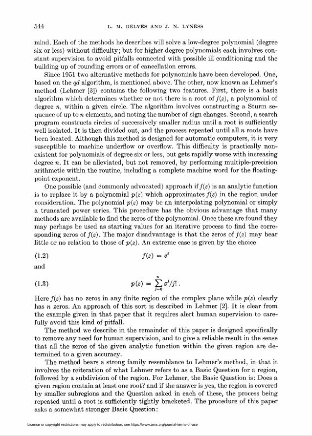
544 L. M. DELVES AND J. N. LYNESS
mind. Each of the methods he describes will solve a low-degree polynomial (degree
six or less) without difficulty; but for higher-degree polynomials each involves con-
stant supervision to avoid pitfalls connected with possible ill conditioning and the
building up of rounding errors or of cancellation errors.
Since 1951 two alternative methods for polynomials have been developed. One,
based on the qd algorithm, is mentioned above. The other, now known as Lehmer's
method (Lehmer [3]) contains the following two features. First, there is a basic
algorithm which determines whether or not there is a root of fiz), a polynomial of
degree n, within a given circle. The algorithm involves constructing a Sturm se-
quence of up to n elements, and noting the number of sign changes. Second, a search
program constructs circles of successively smaller radius until a root is sufficiently
well isolated. It is then divided out, and the process repeated until all n roots have
been located. Although this method is designed for automatic computers, it is very
susceptible to machine underflow or overflow. This difficulty is practically non-
existent for polynomials of degree six or less, but gets rapidly worse with increasing
degree n. It can be alleviated, but not removed, by performing multiple-precision
arithmetic within the routine, including a complete machine word for the floating-
point exponent.
One possible (and commonly advocated) approach if fiz) is an analytic function
is to replace it by a polynomial piz) which approximates fiz) in the region under
consideration. The polynomial piz) may be an interpolating polynomial or simply
a truncated power series. This procedure has the obvious advantage that many
methods are available to find the zeros of the polynomial. Once these are found they
may perhaps be used as starting values for an iterative process to find the corre-
sponding zeros of fiz). The major disadvantage is that the zeros of fiz) may bear
little or no relation to those of piz). An extreme case is given by the choice
(1.2) m = e2
and
(1.3) PÜ0«-Íb*7¿!.
Here fiz) has no zeros in any finite region of the complex plane while piz) clearly
has n zeros. An approach of this sort is described in Lehmer [2]. It is clear from
the example given in that paper that it requires alert human supervision to care-
fully avoid this kind of pitfall.The method we describe in the remainder of this paper is designed specifically
to remove any need for human supervision, and to give a reliable result in the sense
that all the zeros of the given analytic function within the given region are de-
termined to a given accuracy.
The method bears a strong family resemblance to Lehmer's method, in that it
involves the reiteration of what Lehmer refers to as a Basic Question for a region,
followed by a subdivision of the region. For Lehmer, the Basic Question is : Does a
given region contain at least one root? and if the answer is yes, the region is covered
by smaller subregions and the Question asked in each of these, the process being
repeated until a root is sufficiently tightly bracketed. The procedure of this paper
asks a somewhat stronger Basic Question :
License or copyright restrictions may apply to redistribution; see https://www.ams.org/journal-terms-of-use
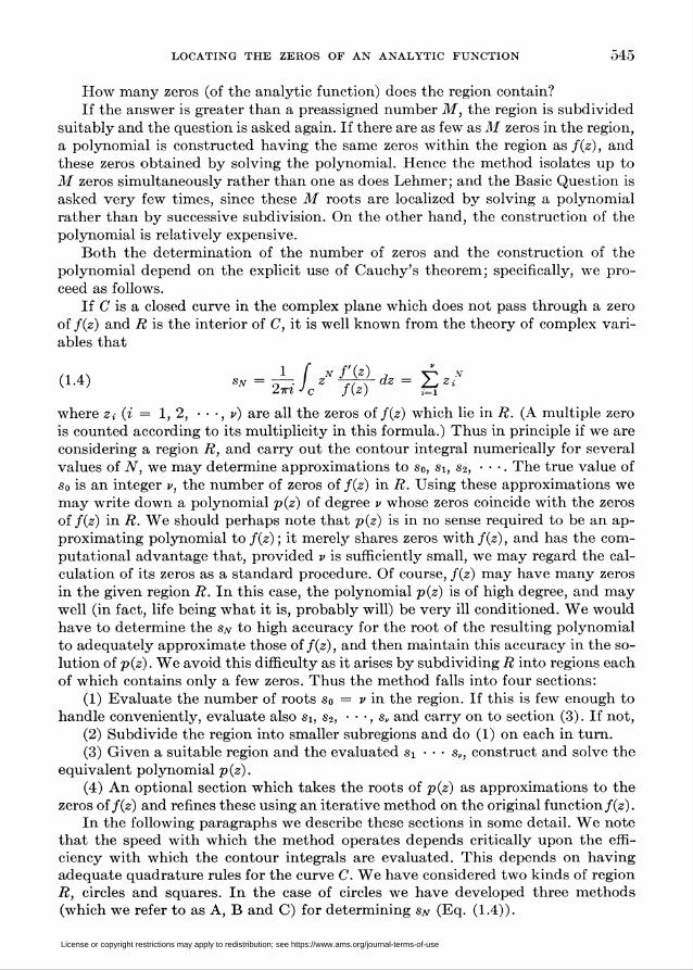
LOCATING THE ZEROS OP AN ANALYTIC FUNCTION 545
How many zeros (of the analytic function) does the region contain?
If the answer is greater than a preassigned number M, the region is subdivided
suitably and the question is asked again. If there are as few as M zeros in the region,
a polynomial is constructed having the same zeros within the region as fiz), and
these zeros obtained by solving the polynomial. Hence the method isolates up to
M zeros simultaneously rather than one as does Lehmer; and the Basic Question is
asked very few times, since these M roots are localized by solving a polynomial
rather than by successive subdivision. On the other hand, the construction of the
polynomial is relatively expensive.
Both the determination of the number of zeros and the construction of the
polynomial depend on the explicit use of Cauchy's theorem; specifically, we pro-
ceed as follows.
If C is a closed curve in the complex plane which does not pass through a zero
of fiz) and R is the interior of C, it is well known from the theory of complex vari-
ables that
(1.4) *» = T--f zNÇ^-dz= ±zY2m Je fiz) tí
where z( (* = 1, 2, • • •, v) are all the zeros of fiz) which lie in R. (A multiple zero
is counted according to its multiplicity in this formula.) Thus in principle if we are
considering a region R, and carry out the contour integral numerically for several
values of N, we may determine approximations to so, Si, S2, * * *. The true value of
So is an integer v, the number of zeros of fiz) in R. Using these approximations we
may write down a polynomial piz) of degree v whose zeros coincide with the zeros
of fiz) in R. We should perhaps note that piz) is in no sense required to be an ap-
proximating polynomial to/(z); it merely shares zeros with/(z), and has the com-
putational advantage that, provided v is sufficiently small, we may regard the cal-
culation of its zeros as a standard procedure. Of course, fiz) may have many zeros
in the given region R. In this case, the polynomial piz) is of high degree, and may
well (in fact, life being what it is, probably will) be very ill conditioned. We would
have to determine the sN to high accuracy for the root of the resulting polynomial
to adequately approximate those of fiz), and then maintain this accuracy in the so-
lution of piz). We avoid this difficulty as it arises by subdividing R into regions each
of which contains only a few zeros. Thus the method falls into four sections:
(1) Evaluate the number of roots s0 = v in the region. If this is few enough to
handle conveniently, evaluate also Si, s2, • • ■, s„ and carry on to section (3). If not,
(2) Subdivide the region into smaller subregions and do (1) on each in turn.
(3) Given a suitable region and the evaluated si • • • s„, construct and solve the
equivalent polynomial piz).
(4) An optional section which takes the roots of piz) as approximations to the
zeros oí fiz) and refines these using an iterative method on the original function fiz).
In the following paragraphs we describe these sections in some detail. We note
that the speed with which the method operates depends critically upon the effi-
ciency with which the contour integrals are evaluated. This depends on having
adequate quadrature rules for the curve C. We have considered two kinds of region
R, circles and squares. In the case of circles we have developed three methods
(which we refer to as A, B and C) for determining sN (Eq. (1.4)).
License or copyright restrictions may apply to redistribution; see https://www.ams.org/journal-terms-of-use

546 L. M. DELVES AND J. N. LYNESS
2. The Basic Subroutine; Method A.
The Organization. We refer to the subroutine which carries out the contour in-
tegration as the basic subroutine. This routine is given:
(i) a contour C;
(ii) a function/(z) and/'(z) analytic on and within this contour;
(iii) a list of the known zeros zi, z2, ■ • •, zk oí fiz) which have so far been obtained;
(iv) constants M, K and e (see below).
The routine attempts to calculate the number of zeros of fiz) within C using trap-
ezoidal rule approximations to the contour integral
(2.1; s0 = ^/4rr<fe.2-Ki Jc fiz)
Since the exact result So is known to be an integer, the accuracy required is low.
We need only determine unambiguously which integer is involved. There are three
possible outcomes. These are
(a) It finds that fiz) becomes unduly small on the contour and takes this to
imply that there is a zero of fiz) close to the contour. In this case the integration
method, if continued, would converge slowly. The routine does not continue the
integration, but returns control to the search routine, which in turn chooses a dif-
ferent contour.
(b) It finds a value of So. On checking the list of known zeros it finds that q of
these lie within the region C, and hence there are s0 — q unknown zeros within C.
If So — q > M it returns control to the search routine.
(c) It proceeds as in (b) but finds a value s0 — q *§ M. It then evaluates the
So — q unknown zeros as follows. It evaluates approximations to the sums of
powers of zeros
(2.2) sN=J^zY, N = 0,1, •••,So-3,¿-i
using trapezoidal rule approximations to the integral
(2.3) sN = ^-.l zN^~dz.2m Jc fiz)
The method of integration is described in more detail below. Since the locations of
the known zeros zi z2 ■ • • zq are available, the sums sN of the powers of the un-
known zeros are
(2.4) sN= J2 zY = sN-J^zY, N = 0,l,---,s0-q.i=q+l i=l
Based on these numbers, a polynomial of degree s0 — q may be constructed, using
Newton's formulas, which has z; (z = q + 1, • • • s0) as zeros. This polynomial is
solved using the polynomial root-finding subroutine.
Local Deflation. We term the process of subtracting the already known zeros
described by (2.4), local deflation. It performs much the same function as does de-
flation for a polynomial; that is, it avoids finding any root twice. However, since
deflation is carried out only over a given region, it does not suffer from the danger
License or copyright restrictions may apply to redistribution; see https://www.ams.org/journal-terms-of-use

LOCATING THE ZEROS OF AN ANALYTIC FUNCTION 547
of accumulation of round-off errors, as does polynomial deflation (Wilkinson [9]).**
Local deflation is not an essential feature of the method described here; if it is
not used, the only consequence is that additional regions may have to be searched.
However, the total time taken depends on the number of regions searched rather
than on the number of zeros. Thus the use of local deflation results in a consider-
able saving of time.
Programming Details. The integration is abandoned under heading (a) if there
is a zero close to the contour, as manifested by the occurrence of a large value of
|/'(z)//(z)|. The value of this function is of order 1/p, where p is the distance from
the contour to the nearest zero. Thus if r\f'iz)/fiz)\ exceeds some pre-set value K,
indicating that p is less than r/K, the current integration is abandoned. Section 7
of (Lyness and Delves) [5], which we refer to as Paper B, is devoted to a discussion
of this point.It is necessary to give the integration routine some convergence criteria for the
integrals sN. We have already noted that s0 need only be evaluated quite crudely.
The routine we have written accepts a set of values Si, s2, • • •, s„ if each agrees with
a previous iterate to within a pre-set constant e.
The routine also requires a number M, the maximum number of zeros which it
is allowed to handle. The choice of M involves a compromise. The effect of increas-
ing M is that fewer regions need be scanned. However, if we choose M too large,
the resulting equivalent polynomial may be ill conditioned. We would then have
to evaluate si, s2, ■ • ■, s„ to too high an accuracy. We have generally chosen M = 5.
Integration Method; Circles. We define C(zo, r) as the circle, center z0 and radius
r, in the complex plane. We translate the origin to the center of this circle and in-
troduce the integration parameter t given by
(2.5) z = zo + r exp i2mt) .
The zeros of /(z) are denoted by
(2.6) Zj = zo + r¡ exp i2mtj) , j = 1, 2, • • • ,
and we find
(2.7) s4= Texr
rf'jzp 4- r exp j2mt))
Since the integrand is a periodic function of t with period 1, an appropriate rule is
the trapezoidal rule. This is discussed in Paper B. Denoting by <£iv(i) the integrand
in (2.7) and using standard functional notation, we define
(2.8) R[m-1]<pN = - ¿ cpJ¿ ) = - ¿ A¿- ) exp i2mNj/m) .m "wf \m/ m f^î \m/
It follows that
(2.9) s—*, = i B-w + ¿ g *4*sr) ■
** We note that deflation as carried out in Lehmer's method is stable.
License or copyright restrictions may apply to redistribution; see https://www.ams.org/journal-terms-of-use

548 L. M. DELVES AND J. N. LYNESS
Thus the integral in each of the (e + 1) calculations depends on the same set of
function evaluations of fiz)/fiz) and, as is usual in trapezoidal rule calculations, in-
creasing the number of points for function evaluation from m to 2m requires only m
additional function evaluations.
We describe the error analysis of this process in Paper B. There it is shown that
asymptotically
(2.10) \R[m'1]cp - l4>\~OiAm)
where |A| < 1. More precisely
(2.11) Ul = max iAi, A2, Af)
where
Ai = max r¡/r , A2 = max r/r,, Ai = r/Rrj<r Tj>r
and R is the distance from z0 of the nearest point at which /(z) is not analytic. The
convergence of the sum to the integral is linear in the usual sense; that is, each addi-
tional function evaluation reduces the error by a constant factor.
Integration Method; Squares. We define sizo, r) as the square whose vertices are
zo + (±1 ± i)r. We use an m-point trapezoidal rule on each side separately, and
eliminate early terms of the asymptotic expansion of the discretization error, fol-
lowing the method of Romberg. It is shown in Paper B that
(2.12) R(m)f -If- c2/m2 + co/m6 + cio/m10 + ■■■ ,
where // stands for the true contour integral and Ä("°/ for the discretization using
the m-point trapezoidal rule for each side. Using m = 1, 2, 4, 8, • ■ •, 2P, it is shown
that after using 2V+2 points the error E is bounded by
(2.13) \E\<r™J'Z K(4p + 2)!4-
(2-rp)2
where 2rp is the shortest distance between any zero of fiz) and a side of the square
and K is a constant. Asymptotically, in terms of the number of points n, the
discretization error is shown in Paper B to be dominated by a term l/n2lo^n as
n —» °o. This is a slower rate of convergence than for the circle.
3. The Search Routine. The search routine is that part of the program which
splits a given region R containing too many zeros, into smaller regions Ri, • • •, R3.
We have investigated only very simple schemes in which Äi, R2, ■ ■ ■, R, have the
same shape as R. The method of subdivision we have used is as follows:
(a) Squares. The square is divided into four as shown in Fig. 1 (a).
(b) Circles. We have adopted Lehmer's subdivision ; that is, we cover the circle
of radius R with nine smaller circles, namely
(1) a concentric circle of radius R/2,
(2) eight circles of radius 5R/12 regularly spaced around the remaining annulus.
This scheme is shown in Fig. 1 (b).
The subregions are then treated in turn in the order indicated by the subroutine.
This order is broken if at any stage the number of zeros in R remaining to be lo-
cated becomes less than or equal to M. In this case the region R is searched again.
License or copyright restrictions may apply to redistribution; see https://www.ams.org/journal-terms-of-use

LOCATING THE ZEROS OF AN ANALYTIC FUNCTION 549
(a) (b)
Figure 1. The method used to subdivide squares and circles. In each case the original region
is represented by the heavy line. Square regions have the advantage that they can be subdivided
without redundancy. On the other hand, more efficient integration rules can be obtained for
circles. The numbers in the subregions denote the order in which they are treated. This order may
be altered if it is apparent that all the roots have been found, or that those remaining can be
found by a faster alternative procedure (see text).
If the basic subroutine indicates that a region R¡ is unsuitable (because a zero
lies close to the boundary) the region is extended.
For the circle this extension is simple; the radius of the current circle is in-
creased. The procedure for squares is more complicated, since these possess com-
mon sides and the program looks ahead to avoid future trouble. A number of dif-
ferent cases arise which are clumsy to describe but easy to implement; a typical
case is shown in Fig. 2, which portrays the rescue operation when trouble is struck
(for the first time) on (an (inside) edge of) the second subregion of a given square.
TROUBLE
-X-y
Figure 2. An example of the algorithm used for avoiding roots near the edge of the square
subregions. In this example, square 1 was successfully treated, and the trouble encountered on an
inner edge of square 2. The program readjusted squares 2, 3, and 4 as shown. As a result a small
area is covered more than once.
License or copyright restrictions may apply to redistribution; see https://www.ams.org/journal-terms-of-use

550 L. M. DELVES AND J. N. LYNESS
An Example. The working of the search routine is illustrated by a practical ex-
ample taken from Lehmer [2]. We choose
fiz) = Jiiz) - Joiz)J2iz) .
This is a real analytic function of z containing a double zero at the origin and four
other complex zeros of the form ±ai ± ia2 inside a square of side 2R = 12, center
the origin. Fig. 3 illustrates how the program located these zeros when it was
allowed to deal with groups of up to three zeros at a time.
6 ZEROS TROUBLE SHIFT EVALUATE ZEROS
Solution of the Equation J,2(Z) -J0(Z) J2(Z) =0.
Figure 3. Steps in the location of the zeros of the function /i2 — JoJ2- The original region
is a square of side 2R = 12, centered at the origin. The position of the zeros is marked with a
cross. That at the origin is a double zero.
After obtaining the equivalent polynomials piz) the routine calculated the zeros
of these to be
ai = 4.466298 , a2 = 1.46747037 ,
which agree with the zeros of fiz) to the number of significant figures shown. In
this example the convergence parameter e for the integrals was set at 10-4.
The Buffer Zone. The user initially specifies some region which he wishes to be
searched for zeros ; if this region is square it is most likely that the search will be
limited to this region. Exceptions will occur if there is a zero close to the boundary
of the square, when the region may be extended to avoid a difficult integration.
If the region is a circle of radius R, it is not true that the specified circle will be
the only region searched. Fig. 1 shows that the process of subdividing the circle will
cause a search over a region outside the required circle. The extent of this 'Buffer
Zone' depends on the number of subdivisions made; that is, on the number of zeros
in the region and its extension. If there are a large number of zeros, the region
actually searched may include points up to a distance 235Ä/172 ~ 10Ä/7 from
the center of the required circle. This feature of the search routine must be kept
in mind. For the methods described here to be valid, the function must be analytic
over the entire region searched, which may exceed the original region.
4. Comparison with Lehmer's Method. The algorithm presented in this paper
may be applied to an arbitrary analytic function. However, an inevitable question
is: if it is given a polynomial, how does it compare with existing methods? In par-
ticular, a comparison with Lehmer's method is of interest. We first look at the
License or copyright restrictions may apply to redistribution; see https://www.ams.org/journal-terms-of-use

LOCATING THE ZEROS OF AN ANALYTIC FUNCTION 551
relative speed of the methods. Since our algorithm spends most of its time evaluat-
ing fiz) for the numerical integration, its speed is determined by the number of
evaluations needed to attain a given accuracy e in these integrations. We saw in
Section 2 that the dependence of e on the number of function evaluations n has the
form
(4.1) e~eoA", Ul < 1 .
That is, the process converges linearly in the number n.
This is the same order of convergence as obtained in Lehmer's method, which
converges linearly in the number of major steps. However, for a polynomial of de-
gree v, each major step in Lehmer's method involves the tabulation of a Sturm
sequence of Oiv) steps, taking of order v2 operations in all. A single function evalua-
tion takes only of order v operations, and hence the time taken by the method of
this paper increases less rapidly with the degree of the polynomial than does
Lehmer's method, although for polynomials of low degree it is considerably slower.
Such low-degree examples are, of course, rather unkind to the method, since if it is
allowed to treat all the zeros at once, it will spend its time re-constituting the orig-
inal polynomial coefficients and then hand these on to a polynomial-solving routine !
On the other hand, it may often be convenient to use the routine for poly-
nomials of high degree G> 12). Two difficulties can arise with polynomials of high
degree. The first difficulty lies in the polynomial itself, which may be very ill con-
ditioned with respect to its coefficients. These must then be carried to multiple pre-
cision in order to define the roots adequately, independently of the method of solv-
ing the polynomial. The second difficulty is the possible occurrence, in a given
method of solution, of extremely large or extremely small numbers which may
underflow or overflow the machine word. This difficulty exists in Lehmer's method ;
for any given choice of precision in the routine, it is possible to construct poly-
nomials for which this will occur. The routine then fails completely to give a solu-
tion. This difficulty does not occur with the method given here, for which all num-
bers generated are automatically of a reasonable size. .
We illustrate these two different points with the following example of a badly
ill-conditioned polynomial of degree 16, taken from Wilkinson [9] and Olver [7].
fiz) = 12501 62561 x1* + 3854 55882 a*16 4- 8459 47696 xu + 2407 75148 xn
+ 2479 26664 x12 + 642 49356 a;11 4- 410 18752 a:10 + 94 90840 x9
(4.2) + 4178260 x8 + 8 37860 x1 + 2 67232 x6 + 44184 x5
+ 10416 x4 + 1288 x3 + 224 x2 + 16 x + 2
Table 1 shows the result when this polynomial is solved to varying degrees of pre-
cision, using the method of this paper, but with no final iteration. The results agree
with those given by Wilkinson, to the precision stated by him. We see that, indeed
it is necessary to define the polynomial to double precision (about 24 decimal places
on our machine) before the more closely spaced roots become stabilized. However,
an accuracy of about 9 significant figures is obtained using only single-precision
working in the routine itself. We gave the polynomial also to a single-precision
version of Lehmer's method, which was available. This routine failed to solve the
equation, due to the overflow difficulty mentioned above, although we used it as
License or copyright restrictions may apply to redistribution; see https://www.ams.org/journal-terms-of-use
552 L. M. DELVES AND J. N. LYNESS
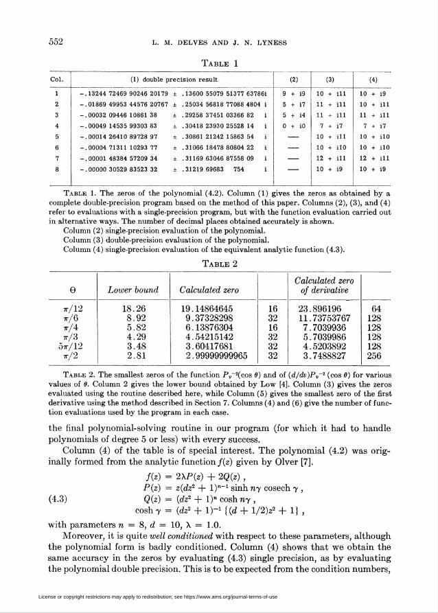
Table 1
Col. (1) double precision result (2) (3) (4)
.13244 72469 90246 20179 ± .13600 55079 51377 63786
.01869 49953 44576 20767 ± .25034 56818 77088 4804
.00032 09446 1086138 ± .29258 3745103366 82
.00049 14535 99303 83 ± .30418 23930 25528 14
.00014 26410 89728 97 ± .3086121242 15863 54
.00004 7131110293 77 ± .31066 18478 80804 22
.0000148384 57209 34 ± .31169 63046 87558 09
.00000 30529 83523 32 ± .31219 69683 754
9 + 19
5 + i7
5 + i4
0 + i0
10 + ill
11 + ill
11 + ill
7 + i7
10 + ill
10 + ilO
12 + ill
10 + i9
10
10
i9
ill
11 + ill
7 + i7
10 + ilO
10 + ilO
12 + ill
10 + i9
Table 1. The zeros of the polynomial (4.2). Column (1) gives the zeros as obtained by a
complete double-precision program based on the method of this paper. Columns (2), (3), and (4)
refer to evaluations with a single-precision program, but with the function evaluation carried out
in alternative ways. The number of decimal places obtained accurately is shown.
Column (2) single-precision evaluation of the polynomial.
Column (3) double-precision evaluation of the polynomial.
Column (4) single-precision evaluation of the equivalent analytic function (4.3).
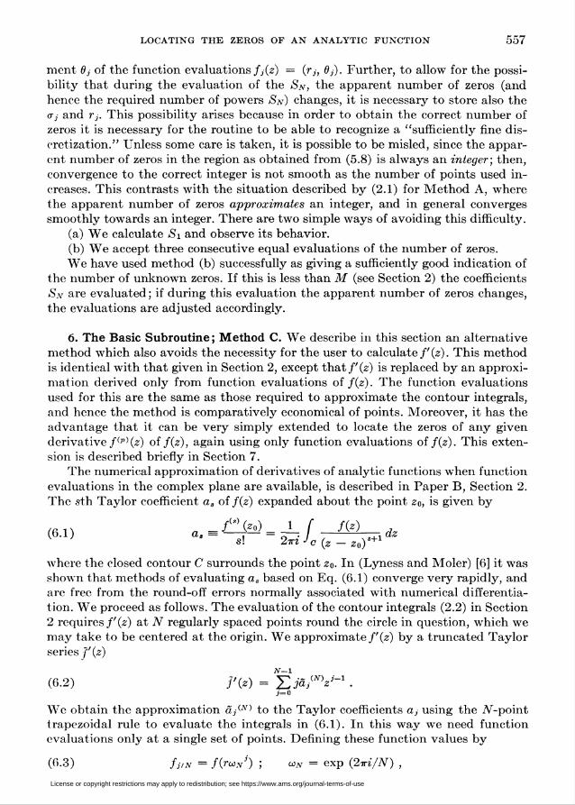
Table 2
e Lower bound Calculated zeroCalculated zero
of derivative
ir/12x/6tt/4tt/3
5ir/12tt/2
18.268.925.824.293.482.81
19.148646459.373282986.138763044.542151423.604176812.99999999965
163216323232
23.89619611.737537677.70399365.70399864.52038923.7488827
64128128128128256
Table 2. The smallest zeros of the function Pv~2(cos 0) and of (d/dv)Pv~2 (cos 0) for various
values of 0. Column 2 gives the lower bound obtained by Low [4]. Column (3) gives the zeros
evaluated using the routine described here, while Column (5) gives the smallest zero of the first
derivative using the method described in Section 7. Columns (4) and (6) give the number of func-
tion evaluations used by the program in each case.
the final polynomial-solving routine in our program (for which it had to handle
polynomials of degree 5 or less) with every success.
Column (4) of the table is of special interest. The polynomial (4.2) was orig-
inally formed from the analytic function/(z) given by Olver [7].
fiz) = 2XP(z) + 2Q(z) ,Piz) = zidz2 + l)"-1 sinh ny cosech y ,
(4.3) Qiz) = idz2 + l)n cosh ny ,
cosh y = idz2 + l)-1 {id + l/2)z2 + 1} ,
with parameters n = 8, d = 10, X = 1.0.
Moreover, it is quite well conditioned with respect to these parameters, although
the polynomial form is badly conditioned. Column (4) shows that we obtain the
same accuracy in the zeros by evaluating (4.3) single precision, as by evaluating
the polynomial double precision. This is to be expected from the condition numbers,
License or copyright restrictions may apply to redistribution; see https://www.ams.org/journal-terms-of-use

LOCATING THE ZEROS OF AN ANALYTIC FUNCTION 553
which for the higher numbered roots are of order unity for (4.3) but 107 for (4.2).
The ability to accept the more natural form (4.3) rather than the derived poly-
nomial is a useful feature of our method; one is given the choice of presenting a
function in the way which makes the zeros the least sensitive to the parameters.
We have demonstrated this ability in an even more striking, although rather
artificial example. The polynomial of degree 20 having as zeros the integers from
1 to 20, has condition number of order 1010 for the larger roots (Wilkinson [9]) and
hence is not represented at all even by a double-precision calculation. The (of course
trivial) representation of this polynomial in terms of its linear factors was given to
the single-precision program, which satisfactorily computed all 20 zeros to at least
nine significant figures.
5. The Basic Subroutine; Method B. The algorithm given in the previous sec-
tion requires the evaluation of the single function fiz)/fiz) at a number of points,
to produce the zeros of fiz). In practice, of course, this will usually involve the
separate evaluation oí fiz) and fiz); and it may happen that the calculation of
fiz) is unduly difficult or takes very much longer than that of fiz). In these circum-
stances it would be convenient to have an algorithm which required only function
evaluation of fiz). We have developed two such methods. The first is derived from
Eq. (5.1) by integrating by parts, and involves the evaluation only of ln/(z); it is
described in this section. An alternative method, involving a numerical approxima-
tion to/'(z), is described in a subsequent section.
We start from Eq. (2.3), which we restate here
(5.1) SN = J2 zY = ~ I zN ¿¡$- dz .2ttî-/c fiz)
Since
(5.2) £&- = - lu fiz) , arg fiz) * - rr,
we see that we can replace the factor fiz)/fiz) by the derivative of In /(z) and
then integrate by parts. The initial difficulty in doing this is that In z is not analytic
within the circle Cr- \z\ = r, but has a branch point at the origin. We therefore
have to be able to keep track of the appropriate sheet on which In /(z) lies as z
passes round the contour C. The possible points of discontinuity in In (z) occur
where arg z = —ir and the main effort in the following analysis goes into ways of
numerically keeping track of these points. We define the principal value of In (z)
as:
In (r exp (2irz7)) = In r + 2mt, -§<íá|,
and in numerical calculations we assume that the subroutine for evaluating the log-
arithm of a complex number calculates this quantity. In what follows, the function
In (z) refers to this principal value.
We assume that no zero oí fiz) lies on the circle \z\ = r. If we define a new w
complex plane, the mapping w = fiz) maps the circle \z\ = r into a closed curve C
in the w plane. This curve does not pass through the origin. We suppose C cuts the
License or copyright restrictions may apply to redistribution; see https://www.ams.org/journal-terms-of-use

554 L. M. DELVES AND J. N. LYNESS
negative real axis at p. distinct points qi, q2, • • *, q„. We assign to each point an
index äy which takes the value +1 or —1 according as C cuts the axis in a positive
(counter clockwise) or in a negative direction. Thus, if the points p¡ in the z plane
correspond to q¡ in the w plane
(5.5) q¡ = fip¡) , arg q¡ = -r,
and for all 0 < ey *g hj, argfip, exp (¿ey)) =-¿ — 7r
(5.6) ¡fy = -sgn (Im/(pyexp (¿Äy))) .
In order to carry out the integration we divide the contour integral C into sec-
tions pip2, p2Pi, • • •■ Within each of these sections arg/(z) ^ —v and so ln/(z) is
continuous. Thus
l-l z»f-^dz=Y-]-P+1zNf-^-dzm L Z f(¿\ dz h 9« h, Z f(z) dZ
(5J) - t Tr-*" ln/(^) Y& ~h\r NzN" ***■/<*)& * N^l,y=i ¿m \pj ¿in Jcr
where the sign on p¡ indicates that the appropriate limit is used. The first term on
the right-hand side may be written
X) viivi)N ■y=i
In the case in which N — 0 we find
(5-8) v = h¡Mdz = %ni'
This corresponds to the well-known result that the number of zeros in Cr is the
number of times C encircles the origin.
For N > 0, the expression
(5.9) S„ = £ wYPif -~l Nz"-1 \nfiz)dzy-i ¿m J cr
is clearly quite unsuitable as a basis for discretization. The locations of p, would
need to be determined and the integral of a function with several discontinuities
would have to be evaluated. To obviate this difficulty we obtain an expression for
2 VjpY in the form of an integral whose discontinuities exactly eliminate those in
the second term. We set
(5.10) pj = r exp (2«Ty)
and we define a function [t] by
[t + l] - M •
An elementary calculation shows that
(5.12) iPjY = 2tíN i (r exp i2mt))N[t - T, - \}dt.J o
Thus we find from (5.9) that
License or copyright restrictions may apply to redistribution; see https://www.ams.org/journal-terms-of-use

LOCATING THE ZEROS OF AN ANALYTIC FUNCTION 555
(5.13) SN = / 2V(rexp i2mt))N<t>it)dtJ o
where
(5.14) <K0 = ¿^ äßm\t - Tj - §] - ln/(r exp (2t»í)) •i
We note that <f>it) is a continuous function of t with period 1. Hence if the values
of Tj were known exactly, the integral would be a priori quite as straightforward
as the original (2.7), the principal difference in the amount of work being that
In [fiz)] is calculated instead oí fiz). We show below that it is not necessary to
know Tj exactly to obtain accurate numerical results. The information that Tj is
chosen so that #(i) is continuous is sufficient.
Discretization. The discretization may be accomplished using an n-point trape-
zoidal rule
(5.15) Rl"'\it) = ^ ± Jj-) .n k=i \ n /
We first define what we term a "sufficiently fine discretization." We require the com-
puter to determine the number of times the curve V:w = fiz), \z\ = r cuts the
negative real w axis, and it has at its disposal only a finite number of points on this
curve. Thus if the curve behaves in an unexpected manner between two successive
points, the routine may fail to indicate this. We define a sufficiently fine discretiza-
tion as follows:
(i) The curve cuts the negative real axis only once or not at all between any
pair of neighboring points.
(ii) The straight line segment connecting these points cuts the negative real
axis the same number of times as the corresponding section of the curve.
The analytic results obtained below all depend on the discretization being suf-
ficiently fine.
We suppose that arg z is defined so that
(5.16) —it < arg z ^ ir.
For a particular discretization we have available the values of fir exp (2irziy)) where
tj = j/n and j = 1,2, • • •, n. We may assign to each point a value of a defined as
follows:
<Tj = +1 , arg/y - arg/y_i ^ -it ,
(5.17) try = 0 , — w < arg/y - arg/y_i *g -k ,
o-y = — 1 , it < arg/y - arg/y_i .
This has the effect that, if Tj lies between tk and i*+i, <xi+i is set equal to ¡7/. In
this respect the discretization transfers properties pertaining to points at which C
cuts the negative real axis to the next calculated point on the curve. We now con-
sider the trapezoidal sum
R[nA][t - Tj - |] exp i2mNt) ,
where
License or copyright restrictions may apply to redistribution; see https://www.ams.org/journal-terms-of-use

556 L. M. DELVES AND J. N. LYNESS
(5.18) tk < Tj < tk+l
and
We find
(5.19)
where
n> N ^ 0
R[n,1]i[t - Tj - }] exp i2mNt)) - - ¿ (<• - Ty + |) exp (2xtM,)71 '=0
+ - Z ih-Tj- |) exp (2«7W,)
(5.20) U = l/n.
Since
i n~*
(5.21) - 31 exp i2mNti) = 0 , n> N ,n i=o
it follows that the terms in T'y in expression (5.19) eliminate each other. The value
of Rln-1][t — Tj — \] exp i2mNt) does not depend on the exact value of Tj, but
only depends on k, that is on the interval in which Tj is situated. A simple calcula-
tion gives
(5.22) R™[t - Tj - %] exp (2*¿OT) = exp '¡2xiA^+1)v ' l j 2j k v / n(exp (2x^A^/n) — 1) '
where T'y lies in the interval tk < Tj *S tk+i and n > N.
The calculation of ¿w may be arranged as follows :
(5.23) SN~NRlnA\<i>it) exp i2mNt)rN) = TNM - L.v(r,)
where
(5.24) LN(n) = NR[n-1]iir exp i2mt))N In fir exp (2tt¿í)))
and
(5.25) TYn) =N32 2mR[nA]ïïj[t - Tj - J](r exp (2«<))" .i
The advantage of doing this is that TV(n) need not be calculated as a trapezoidal
sum. We note that in the discretization a nonzero value of ¡ry is assigned to the next
calculated point; moreover, replacing Tj by the next calculated point does not alter
the value of the trapezoidal sum. Consequently
n
(5.26) Ta/"' =N31 2x¿r* exp (2«Ar4)/n(exp i2mN/n) - 1) .k-l
This relatively simple analytic expression for TYn) is clearly much more convenient
than (5.25).
Programming Details. The final results (5.24) and (5.26) give an alternative way
of evaluating the power sums Sn, and a routine based on these equations can re-
place the basic subroutine described in Section 2. The user need not then evaluate
fiz) at all. In order to evaluate the <r¿ it is necessary to tabulate and store the argu-
License or copyright restrictions may apply to redistribution; see https://www.ams.org/journal-terms-of-use
LOCATING THE ZEROS OF AN ANALYTIC FUNCTION 557
ment 6, of the function evaluations/y(z) = (ry, Of). Further, to allow for the possi-
bility that during the evaluation of the SN, the apparent number of zeros (and
hence the required number of powers Sn) changes, it is necessary to store also the
o-j and ry. This possibility arises because in order to obtain the correct number of
zeros it is necessary for the routine to be able to recognize a ■"sufficiently fine dis-
cretization." Unless some care is taken, it is possible to be misled, since the appar-
ent number of zeros in the region as obtained from (5.8) is always an integer; then,
convergence to the correct integer is not smooth as the number of points used in-
creases. This contrasts with the situation described by (2.1) for Method A, where
the apparent number of zeros approximates an integer, and in general converges
smoothly towards an integer. There are two simple ways of avoiding this difficulty.
(a) We calculate S\ and observe its behavior.
(b) We accept three consecutive equal evaluations of the number of zeros.
We have used method (b) successfully as giving a sufficiently good indication of
the number of unknown zeros. If this is less than M (see Section 2) the coefficients
Sx are evaluated ; if during this evaluation the apparent number of zeros changes,
the evaluations are adjusted accordingly.
6. The Basic Subroutine; Method C. We describe in this section an alternative
method which also avoids the necessity for the user to calculate/'(z). This method
is identical with that given in Section 2, except that/'(z) is replaced by an approxi-
mation derived only from function evaluations of fiz). The function evaluations
used for this are the same as those required to approximate the contour integrals,
and hence the method is comparatively economical of points. Moreover, it has the
advantage that it can be very simply extended to locate the zeros of any given
derivative/(p)(z) oí fiz), again using only function evaluations oí fiz). This exten-
sion is described briefly in Section 7.
The numerical approximation of derivatives of analytic functions when function
evaluations in the complex plane are available, is described in Paper B, Section 2.
The sth Taylor coefficient as oí fiz) expanded about the point zo, is given by
(en a=£U¿fu = J-[ /(«) dz{bA> a>- si 2mhiz-ZoY+i
where the closed contour C surrounds the point z0. In (Lyness and Moler) [6] it was
shown that methods of evaluating as based on Eq. (6.1) converge very rapidly, and
are free from the round-off errors normally associated with numerical differentia-
tion. We proceed as follows. The evaluation of the contour integrals (2.2) in Section
2 requires/'(z) at N regularly spaced points round the circle in question, which we
may take to be centered at the origin. We approximate/'(z) by a truncated Taylor
series/'(z)
(6.2) fiz) = Ziäy^V-1 .y=o
We obtain the approximation ôyw) to the Taylor coefficients ay using the A-point
trapezoidal rule to evaluate the integrals in (6.1). In this way we need function
evaluations only at a single set of points. Defining these function values by
(6.3) fjlN = firoo.Y) ; w.v = exp i2m/N) ,
License or copyright restrictions may apply to redistribution; see https://www.ams.org/journal-terms-of-use
558 L. M. DELVES AND J. N. LYNESS
the required formulas are
1 N(6.4) rsäs(N) = ^ 31 m~sifj,N
1\ y=i
and
JV-l
(6.5) r/'y/iv = ¿^ sr a. aws=0
The trapezoidal rule (6.4) used for approximating as corresponds to the first term
in the expansions given in Lyness and Moler. The truncation error of the ap-
proximation (6.5) for/' is considered in Paper B. This error stems from two sources
—the truncation of the Taylor series at the Ath term, and the approximation used
for the coefficients a, which are retained. In Paper B it is shown that the total
truncation error using N points has the form
(6.6) |r/'(z) - r/'(z)ml < ËN; \z\ -g r,
where
(6.7) ËN ~ const NpN as |2V| -> °o ; 0 < Ipl < 1 .
A more detailed bound is given in Paper B, Eq. (2.6). Eq. (6.7) shows that the
accuracy of the approximation to the derivatives at each point has the same ex-
ponential dependence on N, as the truncation error involved in performing the final
contour integrations using Eq. (2.6).
As in (2.7), the work may be arranged so that in proceeding from N to 2A points
we need only perform operations with the added points. We define coefficients Oy(iV>
involving only these added points :
(6.8) r%m = ± 31 ^-"fvk-vnN , j=l---N.JV k=l
Then in terms of these coefficients we have
,. (2N) _ i, .- GV) , ,, OVK(6.9) rüs -*^°« +r0s >' S = 0---A-1,
Y+Na%N¿ = Wäsm - rV-v)) ,
and
2V-1
(6.10)
j.,(2N) ,,(AT) . At V-> s+N-(.2N) i(«-l) .rft/iw = rftiN |]í¿r al+Nu2N , t even,
s=0N-l iV-1Es, (.N) t(s-l) A7 V^ s+N~'2M i(s-l) . ji
sr bf u2N — N 2-¿r a,+N<¿m , t odd .8=0 s=0
An Example. Both this method and that of the previous section are particularly
easy to use, since the user has only to provide a routine for evaluating /(z). We
demonstrate their power by means of a simple example which was the subject of a
recent paper (Low [4]). This was concerned with the evaluation of the smallest
zeros of the associated Legendre function Pv~m (cos 0) for fixed m and 6, as a func-
tion of v. These zeros are known to be all simple and real, and Low obtained bounds
License or copyright restrictions may apply to redistribution; see https://www.ams.org/journal-terms-of-use
LOCATING THE ZEROS OF AN ANALYTIC FUNCTION 559
on the smallest zeros for m — 2 and a number of values of 0. A program based on
the method of this paragraph was used to search for the smallest zeros, and gave
the results in Table 2.
7. The Zeros of /(p)(z). Method C may be adapted in an obvious manner to ob-
tain the zeros of the pth derivative /(p)(z) of a given analytic function/(z). The cal-
culation of the Taylor coefficients ây(iV) takes place as before, but fiz)/fiz) is re-
placed whenever it occurs by the approximation to/<p+1)(z)//(p)(z) based on these
Taylor coefficients, using
(7.1) fp\z) ^f(p\z) - 31jij - 1) • - - 0" - V + l)äjmY-p .y=o
The truncation error involved in Eq. (7.1) is considered in Paper B. There it is
shown that using N function evaluations
(7.2) rp\fp\z) -f(p\z)\ < ËN(p) ; \z\ Û r,
where
(7.3) ËYP) ~ const NppN , N -> » ; 0 < \p\ < 1.
An Example. As an example of the use of this technique, we consider a problem
due to W. L. Morris (private communication). The following function arises in the
consideration of algorithms for solving sets of ordinary differential equations :
(7 4) f( -= 1 ~ 1005e~' + °-525e~2z - 0-475<T3* - 0.045e~4*
2.27e~* - 2.19e~2* + 1.86e-3z - 0.38e-4*
for which the characteristic of interest is the location of the zero of smallest modulus
oí fiz). A program based on the method described here was used to search for this
smallest zero, and located it to be
(7.5) zo = 0.3430042 4- ¿1.0339458.
This example is interesting since the function (7.4) has a pole at zp:
zp = -0.2275004 ± ¿1.1152220
with modulus only slightly greater than that of zo. This serves to emphasize the re-
marks made in Section 3. The methods given in this paper require a knowledge that
the function /(z) is analytic in the region searched.
8. The Final Iteration. A feature of almost any global method for locating zeros
is that it is uneconomic to find the zeros to high accuracy. Rather, these should be
located to a relatively low accuracy first and then refined by an iterative technique.
This is also true of the method given here, since it is time consuming to evaluate
the contour integrals to high accuracy. We have therefore allowed for a final iterative
stage in all of the methods.
For Method B we have used the secant rule, while for methods A and C we have
used Newton iteration, with the required derivative in Method C being obtained
from the Taylor expansion (6.2). For all of these methods the final accuracy at-
License or copyright restrictions may apply to redistribution; see https://www.ams.org/journal-terms-of-use

560 L. M. DELVES AND J. N. LYNESS
tained depends only on the accuracy with which the function can be evaluated near
the zero. We have also used Newton's method to iterate the pth derivative, obtain-
ing both/(p)(z) and/(p+1)(z) from the Taylor expansion. In this case, the attainable
accuracy depends on the accuracy of the truncated Taylor series.
9. Discussion of the Methods. The methods given in this paper give a practical
means of finding the zeros of an analytic function or of its derivatives, in a given
region. Each method has its own advantages and disadvantages, and it does not
seem possible to single out one as being always preferable. However, we attempt
here to make some comments on their relative virtues.
These methods give the user the choice of searching in squares or in circles. The
search routine for squares is rather more efficient than for circles, yielding much less
overlap (usually, none) when a subdivision occurs. But the integration rules given
are more efficient for circles than for squares. For circles, we have presented three
methods :
Method A. Explicit evaluation of fiz).
Method B. Evaluation of In (/(z)).
Method C. Evaluation of fiz) by interpolation.
Of these three methods, A is by far the most economical of storage space and is
about as fast as Method B. If no derivatives are available, then in general Method
B is faster than Method C, since for large numbers of points the evaluation of the
Taylor coefficients and then the derivatives in Method C is time consuming. How-
ever, Method C has the advantage that it is readily adapted to find the zeros of
the derivatives or the zeros of several derivatives at the same time.
Acknowledgment. We are indebted to Dr. W. B. Gragg for several stimulating
discussions on these topics.
Oak Ridge National Laboratory
Oak Ridge, Tennessee
1. P. Henrici & B. O. Watkins, "Finding zeros of a polynomial by the Q-D algorithm,"
Comm. ACM, v. 8, 1965, pp. 570-574. MR 31 #4172.2. D. H. Lehmer, "The Graeffe process as applied to power series," MTAC, v. 1, 1945, pp.
377-383. MR 7, 84.3. D. H. Lehmer, "A machine method for solving polynomial equations," J. Assoc. Compul.
Mach., v. 8, 1961, pp. 151-162.4. R. D. Low, "On the first positive zero of Py-h2 (cos 0), considered as a function of y,"
Math. Comp., v. 20, 1966, pp. 421-424.5. J. N. Lyness & L. M. Delves, "On numerical contour integration round a closed con-
tour," Math. Comp., v. 21, 1967, pp. 561-577.6. J. N. Lyness & C. B. Moler, "Numerical differentiation of analytic functions," J. SI AM
Numer. Anal, v. 4, 1967, pp. 202-210.7. F. W. J. Olver, "The evaluation of zeros of high-degree polynomials," Phil. Trans. Roy.
Soc. A, v. 244, 1952, pp. 385-415. MR 14, 209.8. H. Rutishauser, "Der Quotienten-Differenzen-Algorithmus," Z. Angew. Math. Phys.,
v. 5, 1954, pp. 233-251. MR 16, 176.9. J. H. Wilkinson, Rounding Errors in Algebraic Processes, Prentice-Hall, Englewood Cliffs,
N. J., 1963. MR 28 #4661.
License or copyright restrictions may apply to redistribution; see https://www.ams.org/journal-terms-of-use