A Numerical Euler-Lagrange Method for Bubble Tower CO2 Dissolution Modelling

D. Legendre1* and R. Zevenhoven2 1, 2 Faculty of Science and Technology, Thermal and Flow Laboratory, Åbo Akademi University, Turku Finland. * Piispankatu 8 FI-20500 Turku, Finland. daniel.legendre@abo.fi Abstract: The present paper proposes an application for an Euler-Lagrangian one-way coupling method in CO2 bubble tower design. A simplified flow field is presented as the basis of this research work for a slice of fluid and a rotating mesh model is presented as the base of the simulation, in this case involving a mixing rotor. A Turbulent Flow interface from Comsol is used. CO2 concentration as function of time and position is studied. Bubble motion is tracked separately in a Lagrangian spherical particle, in this case using the Comsol Particle Tracing module. A link between mass transfer boundary layer and bubble force is established through the mass time derivative of the dissolving bubble, included as the mass change rate of the particle as function of the local Reynolds, Schmidt and Sherwood number of a spherical bubble using mass diffusion theory. Keywords: CO2 Dissolution, mass transfer, Euler-lagrangian coupling, bubble tracking, frozen rotor FEM. 1. Introduction

While the processes taking place in a bubble reactor are simple to describe in a few sentences it is much more difficult to give a physical description that is useful for engineering purposes. A better understanding of a cluster of bubbles dissolving in a liquid where the species transferred reacts with other dissolved species is an interesting engineering challenge that could result in simplifications of upstream or downstream process units. An example could be being able to predict, for a certain gas/liquid combination, the maximum gas flow that would result in complete dissolution (and chemical conversion). It would allow for operating without a gas outlet for cases where no gaseous products are generated. This is the topic addressed in this paper, where CO2 is dispersed in an aqueous solution that contains dissolved calcium (Ca2+ ions), producing PCC, precipitated calcium carbonate (CaCO3) Fig. 1. (Mattila and

Zevenhoven, 2014) [1] Since the solution used also contains dissolved ammonia (NH3 (aq)) with a certain vapour phase, an exit stream of unreacted CO2 would also contain NH3, which would require an additional separation step to the process for its recovery.

Figure.1 Slag2PCC experimental set up [1]

2. Fluid environment

The first stage to model a bubble tower is to define the moving environment of the surrounding liquid. Taking into account the dimensions for the stirred tank reactor presented by Mattila and Zevenhoven [1] a modification of the geometry was made with the sole objective to enhance bubble dissolution. The goal is to study the critical height of bubble dissolution for a defined initial bubble size in a given solution. Impeller dimensions are defined according the standard tank geometry parameters [2]. The mineral carbonation process [1] requires a constant mixing environment to maintain the suspensions of Ca2+ ions in the fluid that are a crucial part of the slag2PCC process. The CO2

dissolution emanates from a flow stream of small spheroidal bubbles, as it is know that a larger area gives a larger mass transfer effect.

A simplified flow field is presented as the

basis of this research work for a slice of fluid and a rotating mesh model is presented as the base of the fluid flow field. A Turbulent Flow interface

Excerpt from the Proceedings of the 2015 COMSOL Conference in Grenoble

from Comsol is used. As initial conditions for a time dependent solver the flow field is obtained from a Frozen Rotor simulation. Due to computational power limitations (CPU core i7 with 16 GB RAM) the simulated section of length ‘’L’’ (also the distance between several subsequent impellers) is stacked to form the total bubble tower (Fig 2). As a first approach the problem will center in a section of this bubble tower.

2.1 Boundary conditions

The system consist of a section of a vertical

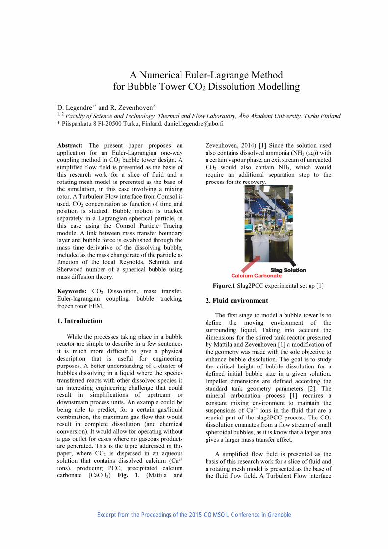
pipe of diameter [D1= 127 mm] with an internal cylindrical rotating domain that contains the impeller geometry with varying diameter of 50-75% of the outer pipe (Fig. 1). These domains are joined by an identity pair and on both a gravitational force acts as a volumetric force in the –z direction. Impeller shaft velocity outside the rotating domain is modelled as a moving wall with velocity Ω x R, with “Ω” the rotational speed and “R” the radial coordinates of the shaft. The liquid is water under ambient conditions and taking advantage of the periodicity of the bubble tower the bottom and top faces are constrained to be periodic. To improve convergence a constrain point of pressure Po=0 is put at the top of the outer domain. The fluid dynamic environment can be observed in Fig 2.

Figure 1. Rotating domain

Figure 2. Section of the bubble tower simulated

and boundary conditions (Velocity w).

2.2 Frozen rotor simulation

A rotational flow simulation in a mixer is characterized to be a time dependent phenomenon as the flow field presents certain oscillatory behavior. For reactors with suspended particles the widely accepted perfect mixing assumption is used for design purposes and furthermore validated with experimental results. In fluid dynamics terms perfect mixing implies continuous suspension and particle movement through the entire reactor domain, i.e. particle concentration should be relatively constant in every volume section of the domain. In terms of equipment usage the steady state solution is of interest for reactors, therefore the transitory solution is often neglected.

This modeling work aim at a fully developed

fluid mixing environment for bubble dissolution, consequently a Frozen Rotor simulation using a finite element method in an Eulerian framework is used as an initial condition for a time dependent solution. This implies that the steady state solution can be more rapidly reached numerically in comparison with the calculation of the transitory solution and further stabilization into a steady state solution.

2.3 Time dependent solution

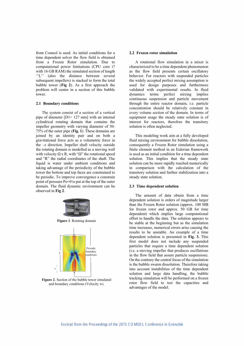
The amount of data obtain from a time dependent solution is orders of magnitude larger than the Frozen Rotor solution (approx. 100 MB for frozen rotor and approx. 50 GB for time dependent) which implies large computational effort to handle the data. The solution appears to be stable at the beginning but as the simulation time increases, numerical errors arise causing the results to be unstable. An example of a time dependent solution is presented in Fig. 3. This first model does not include any suspended particles that require a time dependent solution (i.e. a moving impeller that produces oscillations in the flow field that assure particle suspension). On the contrary the central focus of the simulation is the bubble swarm dissolution. Therefore taking into account instabilities of the time dependent solution and large data handling, the bubble tracking simulation will be performed on a frozen rotor flow field to test the capacities and advantages of the model.

Excerpt from the Proceedings of the 2015 COMSOL Conference in Grenoble

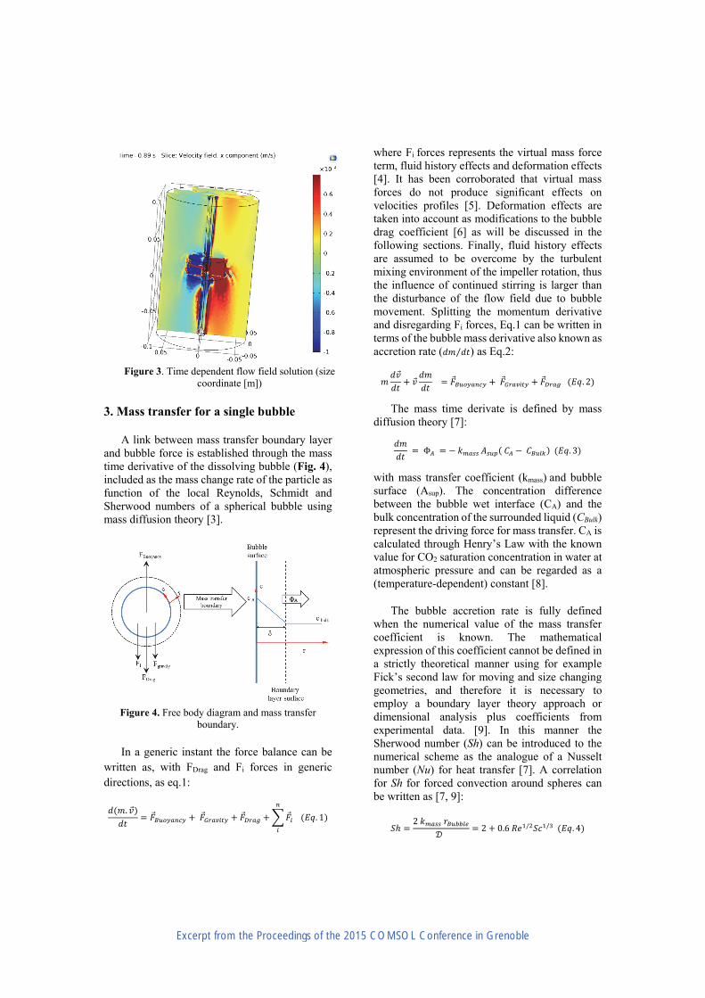
Figure 3. Time dependent flow field solution (size coordinate [m])

3. Mass transfer for a single bubble

A link between mass transfer boundary layer and bubble force is established through the mass time derivative of the dissolving bubble (Fig. 4), included as the mass change rate of the particle as function of the local Reynolds, Schmidt and Sherwood numbers of a spherical bubble using mass diffusion theory [3].

Figure 4. Free body diagram and mass transfer boundary.

In a generic instant the force balance can be

written as, with FDrag and Fi forces in generic directions, as eq.1:

. . 1

where Fi forces represents the virtual mass force term, fluid history effects and deformation effects [4]. It has been corroborated that virtual mass forces do not produce significant effects on velocities profiles [5]. Deformation effects are taken into account as modifications to the bubble drag coefficient [6] as will be discussed in the following sections. Finally, fluid history effects are assumed to be overcome by the turbulent mixing environment of the impeller rotation, thus the influence of continued stirring is larger than the disturbance of the flow field due to bubble movement. Splitting the momentum derivative and disregarding Fi forces, Eq.1 can be written in terms of the bubble mass derivative also known as accretion rate ( ⁄ ) as Eq.2:

. 2

The mass time derivate is defined by mass diffusion theory [7]:

Φ . 3

with mass transfer coefficient (kmass) and bubble surface (Asup). The concentration difference between the bubble wet interface (CA) and the bulk concentration of the surrounded liquid (CBulk) represent the driving force for mass transfer. CA is calculated through Henry’s Law with the known value for CO2 saturation concentration in water at atmospheric pressure and can be regarded as a (temperature-dependent) constant [8].

The bubble accretion rate is fully defined when the numerical value of the mass transfer coefficient is known. The mathematical expression of this coefficient cannot be defined in a strictly theoretical manner using for example Fick’s second law for moving and size changing geometries, and therefore it is necessary to employ a boundary layer theory approach or dimensional analysis plus coefficients from experimental data. [9]. In this manner the Sherwood number (Sh) can be introduced to the numerical scheme as the analogue of a Nusselt number (Nu) for heat transfer [7]. A correlation for Sh for forced convection around spheres can be written as [7, 9]:

2

2 0.6 / / . 4

Excerpt from the Proceedings of the 2015 COMSOL Conference in Grenoble

where the Schmidt number (Sc) and Reynolds number (Re) are defined as:

. 5

2 | |

. 6

with diffusion coefficient D for CO2 dissolved in water for bubble of radius rbubble and relative velocity | | respective to the surrounded liquid with kinetic and dynamic viscosity υfluid and μfluid.

3.1 Chemical reaction effects

The Hatta number (Ha) is a dimensionless number that compares the rate of reaction in a liquid film (in general: a boundary layer) to the rate of diffusion through that film, here defined as:

. 7

where the chemical reaction rate for reacting CO2

in presence of dissolved calcium (kreaction) has been defined experimentally by Mattila et al. [10].

After some mathematical rearranging for the accretion rate defined by mass transfer theory via the boundary layer thickness δ for first order chemical reaction [11] the mass derivative is written as:

1 . 8

3.2 Spherical shape deviation effects

Bubble deformation effects are taken into account as modifications to the drag coefficient using Eötvös (Eo), Morton (Mo) and Reynolds (Re) number relations for rising bubbles according to studies by Roghair et al. 2011 [6]:

. 9

with:

16

12

1 16 3.315√

. 10

4

9.5 . 11

The dimensionless numbers Mo and Eo are defined as:

2 . 12

. 13

with surface tension σ. Finally the expected bubble shape can be tracked in the shape regime map for bubbles in liquids with Re, Mo and Eo relations according to Amaya-Bower and Lee [12].

4. Bubble Lagrangian tracking

Bubble motion is tracked separately for a Lagrangian spherical particle as a similar approach to Jamshidi and Brenner [13], in this case using the Comsol Particle Tracing module. For this particular case the bubble radius change is produced by mass diffusion, chemical reaction effects and local pressure changes in the fluid. Jamshidi and Brenner [13] proved that a variable bubble size motion can be simulated without serious numerical convergence complications.

4.1 Initial conditions

The bubble while rising is expected to have a Re of an order of magnitude of 103 [1], therefore assuming regime in which Stokes Law (Re << 1) drag coefficients will have large discrepancies with the experimental drag coefficients for that Reynolds number range. An initial velocity is needed and according to Michaelides [4] for high Reynolds numbers a constant value CD high Re of 0.43 is recommended.

It is therefore preferable to define as an initial rise bubble speed the speed that a bubble would have for large Reynolds numbers, as high Reynolds flow would be a better estimation for rising bubbles than Stokes Law. We can determine this initial steady velocity with a force balance between drag and buoyancy forces for non-accelerating bubbles as:

83

. 14

Excerpt from the Proceedings of the 2015 COMSOL Conference in Grenoble

Bubble initial radius and mass define the initial conditions of the bubble and density is calculated using the ideal gas equation at ambient conditions. Local pressure is found from the pressure field obtained from the fluid dynamic simulation.

5. Euler-Lagrangian one-way coupling in COMSOL Multiphysics

Here a one-way coupling is used in contrast with the two-way coupling used by Gong et al. [14] for mass transfer of ozone dissolution in bubble plumes. In their case the fluid (water) remained stagnant without any momentum source that modified the flow field apart from bubble displacement. In a stirred reactor it is necessary to maintain certain momentum intake from a moving impeller, as a turbulent fluid environment that induces mixing and recirculation patterns is desired. It is assumed that the amount of energy imparted by the impeller is far superior to the flow pattern disturbing effects of the rising bubbles. Two-way coupling is more computational demanding than one-way coupling as the different physics are not connected, thus resulting in smaller systems of equations to solve. In this sense a one way coupling represents a more suitable solution within the limits of computer use. 5.1. Model assembly in COMSOL

The model is decomposed in two different solvers. First a frozen rotor with a mesh calibrated for fluid dynamics with an approximate number of 2 million elements for the different heights of the bubble towers modelled. Corner refinement on the moving impeller domain and boundary layer elements on the wall of the reactor wall are used. After the fluid environment is defined, it is used as base for a time-dependent solver for bubble Lagrangian tracking as a one-way coupling multiphysics problem.

6. Flow field simulation results

Different simulations where performed for different combination of parameters Ω and L. Results for a rotational speed Ω =100 rpm and L=50 cm are presented in Fig. 4.

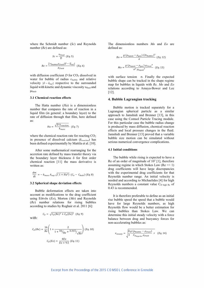
Figure 4. Velocity field z (vertical) and x (radial) The mixing pattern in the bubble column

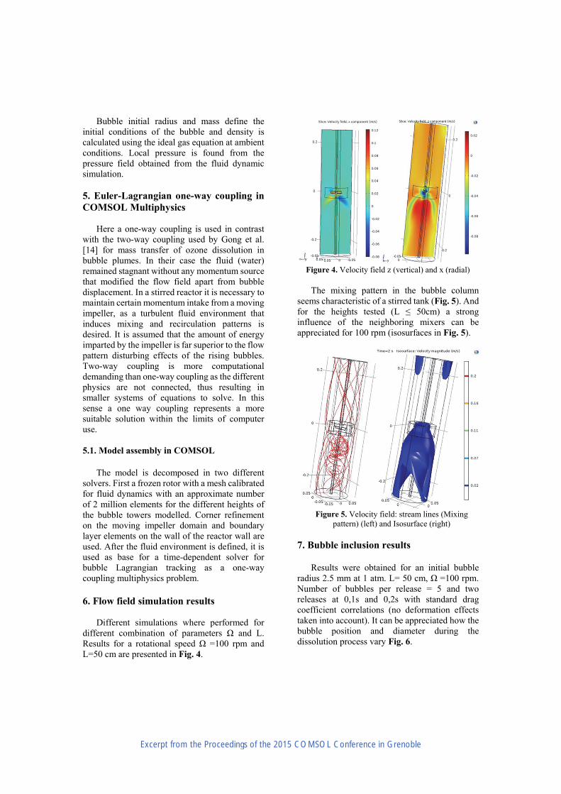
seems characteristic of a stirred tank (Fig. 5). And for the heights tested (L ≤ 50cm) a strong influence of the neighboring mixers can be appreciated for 100 rpm (isosurfaces in Fig. 5).

Figure 5. Velocity field: stream lines (Mixing pattern) (left) and Isosurface (right)

7. Bubble inclusion results

Results were obtained for an initial bubble radius 2.5 mm at 1 atm. L= 50 cm, Ω =100 rpm. Number of bubbles per release = 5 and two releases at 0,1s and 0,2s with standard drag coefficient correlations (no deformation effects taken into account). It can be appreciated how the bubble position and diameter during the dissolution process vary Fig. 6.

Excerpt from the Proceedings of the 2015 COMSOL Conference in Grenoble

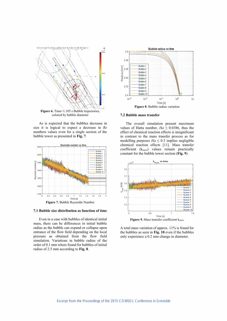
Figure 6. Time=1.105 s Bubble trajectories, colored by bubble diameter

As is expected that the bubbles decrease in

size it is logical to expect a decrease in Re numbers values even for a single section of the bubble tower as presented in Fig. 7.

Figure 7. Bubble Reynolds Number 7.1 Bubble size distribution as function of time

Even in a case with bubbles of identical initial mass, there can be differences in initial bubble radius as the bubble can expand or collapse upon entrance of the flow field depending on the local pressure as obtained from the flow field simulation. Variations in bubble radius of the order of 0.1 mm where found for bubbles of initial radius of 2.5 mm according to Fig. 8.

Figure 8. Bubble radius variation 7.2 Bubble mass transfer

The overall simulation present maximum values of Hatta number, Ha ≤ 0.0386, thus the effect of chemical reaction effects is insignificant in contrast to the mass transfer process as for modelling purposes Ha ≤ 0.3 implies negligible chemical reaction effects [11]. Mass transfer coefficient (kmass) values remain practically constant for the bubble tower section (Fig. 9).

Figure 9. Mass transfer coefficient kmass

A total mass variation of approx. 11% is found for the bubbles as seen in Fig. 10 even if the bubbles only experience a 0.2 mm change in diameter.

Excerpt from the Proceedings of the 2015 COMSOL Conference in Grenoble

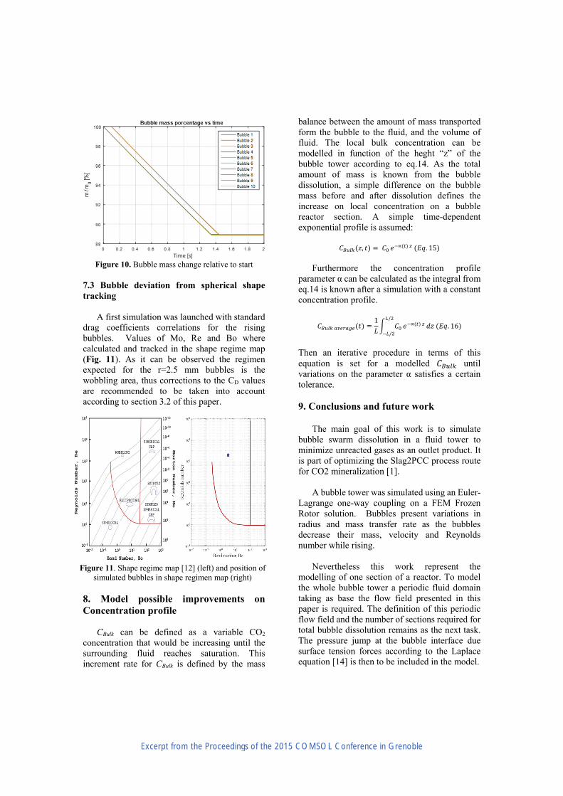
Figure 10. Bubble mass change relative to start 7.3 Bubble deviation from spherical shape tracking

A first simulation was launched with standard drag coefficients correlations for the rising bubbles. Values of Mo, Re and Bo where calculated and tracked in the shape regime map (Fig. 11). As it can be observed the regimen expected for the r=2.5 mm bubbles is the wobbling area, thus corrections to the CD values are recommended to be taken into account according to section 3.2 of this paper.

Figure 11. Shape regime map [12] (left) and position of simulated bubbles in shape regimen map (right)

8. Model possible improvements on Concentration profile

CBulk can be defined as a variable CO2 concentration that would be increasing until the surrounding fluid reaches saturation. This increment rate for CBulk is defined by the mass

balance between the amount of mass transported form the bubble to the fluid, and the volume of fluid. The local bulk concentration can be modelled in function of the heght “z” of the bubble tower according to eq.14. As the total amount of mass is known from the bubble dissolution, a simple difference on the bubble mass before and after dissolution defines the increase on local concentration on a bubble reactor section. A simple time-dependent exponential profile is assumed:

, ∝ . 15

Furthermore the concentration profile

parameter α can be calculated as the integral from eq.14 is known after a simulation with a constant concentration profile.

1

∝

/

/ . 16

Then an iterative procedure in terms of this equation is set for a modelled until variations on the parameter α satisfies a certain tolerance. 9. Conclusions and future work

The main goal of this work is to simulate bubble swarm dissolution in a fluid tower to minimize unreacted gases as an outlet product. It is part of optimizing the Slag2PCC process route for CO2 mineralization [1].

A bubble tower was simulated using an Euler-

Lagrange one-way coupling on a FEM Frozen Rotor solution. Bubbles present variations in radius and mass transfer rate as the bubbles decrease their mass, velocity and Reynolds number while rising.

Nevertheless this work represent the modelling of one section of a reactor. To model the whole bubble tower a periodic fluid domain taking as base the flow field presented in this paper is required. The definition of this periodic flow field and the number of sections required for total bubble dissolution remains as the next task. The pressure jump at the bubble interface due surface tension forces according to the Laplace equation [14] is then to be included in the model.

Excerpt from the Proceedings of the 2015 COMSOL Conference in Grenoble

10. References 1. Mattila H-P. and Zevenhoven R. “Design of

a continuous process setup for precipitated calcium carbonate production from steel converter slag”, ChemSusChem, 3 903-13 (2014).

2. Cheremisinoff N.P. “Handbook of chemical processing equipment”. Butterworth-Heinemann, USA (2000).

3. Bird R. B. “Transport phenomena”. John Wiley & Sons, Inc, USA (2007)

4. Michaellides E.E. “Particles, bubbles and drops”, World Scientific Publishing Co. Pte. Ltd, Singapore (2006)

5. Ashraf Ali B. and Pushpavanam S. “Hydrodynamics, mixing and reaction in bubble columns”. PhD thesis, India, Scholar’s Press (2014)

6. Roghair I. et al. “On the drag force of bubbles in bubble swarms at intermediate and high Reynolds numbers”, Chem. Eng. Sci. 66 3204-3211 (2011).

7. McCabe W.L. et al. “Unit operations of chemical engineering”. McGraw-Hill, New York (1993)

8. Atkins P.W. “Physical chemistry” Oxford University Press, London (1983).

9. Hanjalić K. et al. “Analysis and modelling of physical transport phenomena” VSSD, Delft, the Netherlands (2007)

10. Mattila H-P. et al. “Chemical kinetics modeling and process parameter sensitivity for precipitated calcium carbonate production from steelmaking slags” Chem. Eng. J., 192 77-89 (2012).

11. Beek, W.J. et al. “Transport phenomena” Wiley, USA (1999)

12. Amaya-Bower L. and Lee T. “Single bubble rising dynamics for moderate Reynolds number using Lattice Boltzman Method”, Comp. & Flu. 39 (1191-1207) (2010)

13. Jamshidi R. and Brenner G. “An Euler-Lagrange method considering bubble radial dynamics for modelling sonochemical reactors” Ult. Chem. 21, 154-161 (2013)

14. Gong X, et al. “A numerical study of mass transfer of ozone dissolution in bubble plumes with an Euler-Lagrange method” Elsevier Chem. Eng. Sci. 62, 1081-1093 (2006)

11. Acknowledgements This work was funded by the Doctoral Program in Energy Efficiency and Systems (EES) of Finland (2012-2015) and the Cleen Oy Carbon Capture and Storage Program CCSP (2011-2016).

Excerpt from the Proceedings of the 2015 COMSOL Conference in Grenoble