Numerical Approach and Analytical Study of Cracks Severity ...

Third Serbian (28th Yu) Congress on Theoretical and Applied Mechanics Vlasina lake, Serbia, 5-8 July 2011 C-29
A NUMERICAL APPROACH FOR THE SEISMIC ANALYSIS OF REINFORCED CONCRETE STRUCTURES ENVIRONMENTALLY DAMAGED AND CABLE-STRENGTHENED
A.A. Liolios 1, K.E. Chalioris 1 and K.A. Liolios 2 1 Democritus University of Thrace, Dept. Civil Engineering, Division of Structural Engineering, GR-67100 Xanthi, Greece (e-mail: [email protected]) 2 University of Thrace, Dep. Environmental Engineering, Lab. Ecological Mechanics and Technology, Xanthi, Greece (e-mail: [email protected])
Dedicated to the Memory of Prof. Panagiotis D. Panagiotopoulos, (1.1.1950-12.8.1998),
Late Professor of Aristotle-University of Thessaloniki, Greece.
Abstract. The paper deals with a numerical analusis for the seismic response of reinforced concrete structures containing cable elements. The cable behaviour is considered as nonconvex and nonmonotone one and is described by generalized subdifferential relations including loosening, elastoplastic - fracturing etc. effects. The problem is treated incrementally by double discretization: in space by finite elements and piece-wise linearization of cable - behaviour, and in time by the Newmark method. Thus, in each time - step an incremental linear complementarity problem is solved with a reduced number of problem unknowns. Finally, an example from civil engineering praxis is presented and some results are discussed.
Keywords: Solid Mechanics, Dynamic Unilateral Problems, Cable-braced Structures, optimization algorithmes.
1. Introduction Braces play an important role for the strengthening, repair and earthquake resistant design and construction, see e.g. [1],[2]. This holds especially for reinforced concrete structures, exposed to environmental actions and requiring a strengthening procedure to continue to be serviceable. So, the seismic analysis of braced-structures, such as framing systems, suspended roofs and bridges, offshore platforms and braced towers, is an active investigation field [3],[4],[5]. A special class of braced structures are those containing cable elements. The peculiarity is that these elements can transmit tensile stresses only. The so-caused nonnegativity inequality for cable stresses is the principal condition in the relevant mathematical formulation of the problem. This is nonlinear, not only because of the presence of stress
590

Third Serbian (28th Yu) Congress on Theoretical and Applied Mechanics Vlasina lake, Serbia, 5-8 July 2011 C-29
inequalities, but also because the considered cable stress-strain law is nonlinear, non-convex and non-monotone. Thus, the formulated theory is a large displacement inequality theory, as usual in cable-structures, see e.g. Panagiotopoulos [3], [6] . A compact mathematical treatment of the static problem of cable-structures has been also presented by Panagiotopoulos [3], [7], on the basis of the variational or hemivariational inequality approach. As well known, the hemivariational inequality concept has been introduced into Mechanics and Applied Mathematics by P.D. Panagiotopoulos for first time in 1983, see [8], and constitutes now the basis of the so-called Non-Smooth Mechanics. Further, as concerns numerical aspects, a remarkable approach to the above inequality problem has been obtained by piece-wise linearization of the cable constitutive laws and by using mathematical programming [3], [4], [5], [12]. The aim of this paper is to present a numerical analysis to the seismic problem of cable braced reinforced concrete structures. For this purpose we use a double discretization. First the problem is discretized in space by the finite element method and by piece-wise linearization of the constitutive laws of cable-elements. Then, due to large cable deformations, the problem is given an incremental formulation. Further, a time discretization is applied by using the Newmark method. In each time-step an incremental non-convex linear complementarity problem, with reduced number of unknowns, is formulated and solved. Finally, the developed numerical procedure is applied to a practical Civil Engineering example.
2. Problem formulation The structural system is discretized in space by using finite elements of the "natural" type, see e.g. [3],[6],[14]. Pin-jointed bar elements are used for the cables. The behaviour of these elements includes loosening, elastoplastic or/and elastoplastic-softening-fracturing and unloading - reloading effects. All these characteristics can be expressed mathematically by the relation:
i i i iˆs (d ) S (d ) . (1)
where si and di are the (tensile force) and the deformation (elongation), respectively, of the
i-th cable element, is the generalized gradient and Si is the superpotential function, see Panagiotopoulos [7], [8]. By definition, relation (1) is equivalent to the following hemivariational inequality expressing the Virtual Work Principle:
i i i i i i i iS (d ,e d ) s (d ) (e d ) . (2)
where iS denotes the subderivative of Si and ei, di are kinematically admissible (virtual)
deformations. From the mathematical point of view, using (l) and (2), we can formulate the problem as a hemivariational inequality one by following [7] and investigate it. Instead of this, and because here we are interested for the computational treatment of the problem, we proceed directly by piece wise linearizing the constitutive relations (l). So, in a way similar to that in elastoplasticity –see e.g. Maier [5],[6] - and in unilateral elastodynamics –see e.g. Liolios
591

Third Serbian (28th Yu) Congress on Theoretical and Applied Mechanics Vlasina lake, Serbia, 5-8 July 2011 C-29
[9]-, we have the following constitutive relations (in matrix notation, underlined symbols) for the cable elements:
Tψ B σ Aυ r, (r 0) . (3)
Tψ 0, υ 0, ψ υ 0 . (4a,b,c)
Here σ is the stress vector of the whole structural system; B is a transformation matrix; A is the current symmetric interaction matrix; and ψ, (-υ), r are the yield, slackness and ultimate capacity (resistance), respectively, vectors of cable elements. The remaining constitutive relations for the unassembled structural system are:
e ε Bυ θ . (5)
-1σ E ε or ε E σ . (6)
where e, ε, θ are the total, pure elastic and imposed (e.g. thermal or dislocations) strain vectors, respectively, and E is the current elasticity matrix, symmetric and positive definite. Next, dynamic equilibrium and compatibility for the assembled structural system are expressed, respectively, by the relations
GG σ + K u = p - Cu - Mu . (7)
Te = G u . (8)
Here G is the equilibrium matrix and GT , its transposed, is the compatibility matrix; u and p are the displacement and the load vectors, respectively; C and M are the damping and mass matrices, respectively, both symmetric and in general positive (semi)- definite. The geometric stiffness matrix KG depends linearly on preexisting constant load [6]. Through the term KGu alone the geometry changes affect the equilibriumn (second order geometric effects). As usua1, dots over symbols denote derivatives with respect to time. On the other hand, for the case of seismic excitation, it is
gp = -M x . (9)
where xg(t) is the ground seismic displacement. Finally, the initial conditions are
u(t 0) u , u(t 0) u , υ(t 0) υo o o . (10a,b,c)
where uo, uo and υo are known quantities.
Thus the problem consists in finding the response set {σ(t), u(t), ε(t); ψ(t), υ(t)} which satisfies (3)-(10) for the given excitation set {p(t), -or xg(t)-, θ(t), uo, uo , υo}.
3. The Incremental Linear Complementarity Approach
592
Third Serbian (28th Yu) Congress on Theoretical and Applied Mechanics Vlasina lake, Serbia, 5-8 July 2011 C-29
Due to nonmonotone and nonconvex cable behaviour (large deformations, loosening, elastoplastic-softening-fracturing effects, unloading-reloading etc.), E and A depend on u and υ, respectively. Therefore, an incremental formulation for the problem is more suitable. For this purpose, let Et, At, ψ(t), υ(t) etc. denote known quantities at the time t and let Δt be the time increment. Then the linear complementarity conditions (4) at the next time-moment (t + Δt) are written as follows:
Tt tt t
ψ + Δψ 0 , υ + Δυ 0 , (ψ + Δψ) υ + Δυ = 0 . (11a,b,c)
Next, the remaining problem conditions (3), (5)-(8) take the incremental form
TtΔψ B Δσ A Δυ . (12)
Δe Δε BΔυ Δθ . (13)
-1t tΔσ E Δε or Δε E Δσ . (14)
GΔσ + K Δu = Δp - C Δu - M Δu . (15)
TΔe = G Δu . (16)
Further, we use a time discretization scheme for the step-by-step solution of problem (11)-(l6). As known - see e.g. [10], for implicit time integration methods, relations of the following form hold:
1Δu = c Δu + a . (17a)
2Δu = c Δu + b . (17b)
where c1 and c2 are positive constants in terms of Δt, and a, b known quantities from previous time-steps. So, for the constant-average acceleration method, which is chosen here from the Newmark time-integration schemes, we have
1 22
4 2c , c
ΔtΔt . (17c,d)
In order to reduce the unknowns number, we substitute (l7) into (l5) and eliminate Δσ, Δε, Δe, Δu from (l2)-(l6). So we eventually arrive at
Δψ = Λ Δυ + λ . (18)
where
T -1 TΛ = H K H - A - B E B . (19a)
H = G E B . (19b)
TG 2 1K = G E G + K + c C + c M . (19c)
T -1 Tλ = H K (Δf + C b + M a) - B E Δθ . (19d)
593
Third Serbian (28th Yu) Congress on Theoretical and Applied Mechanics Vlasina lake, Serbia, 5-8 July 2011 C-29
Δf = Δp + G E Δθ . (19e)
Now, (18) with (11) constitute a Linear Complementarity Problem (LCP). In comparison to problem of (1)-(10), the LCP has a reduced number of unknowns. The LCP is solved in terms of the increments Δψ and Δυ by available computer codes of mathematical programming, see [5], [6], [7], [13]. Finally, by using Euler relations u = ut + Δu, υ = υt + Δυ etc., we complet the solution at time (t + Δt).
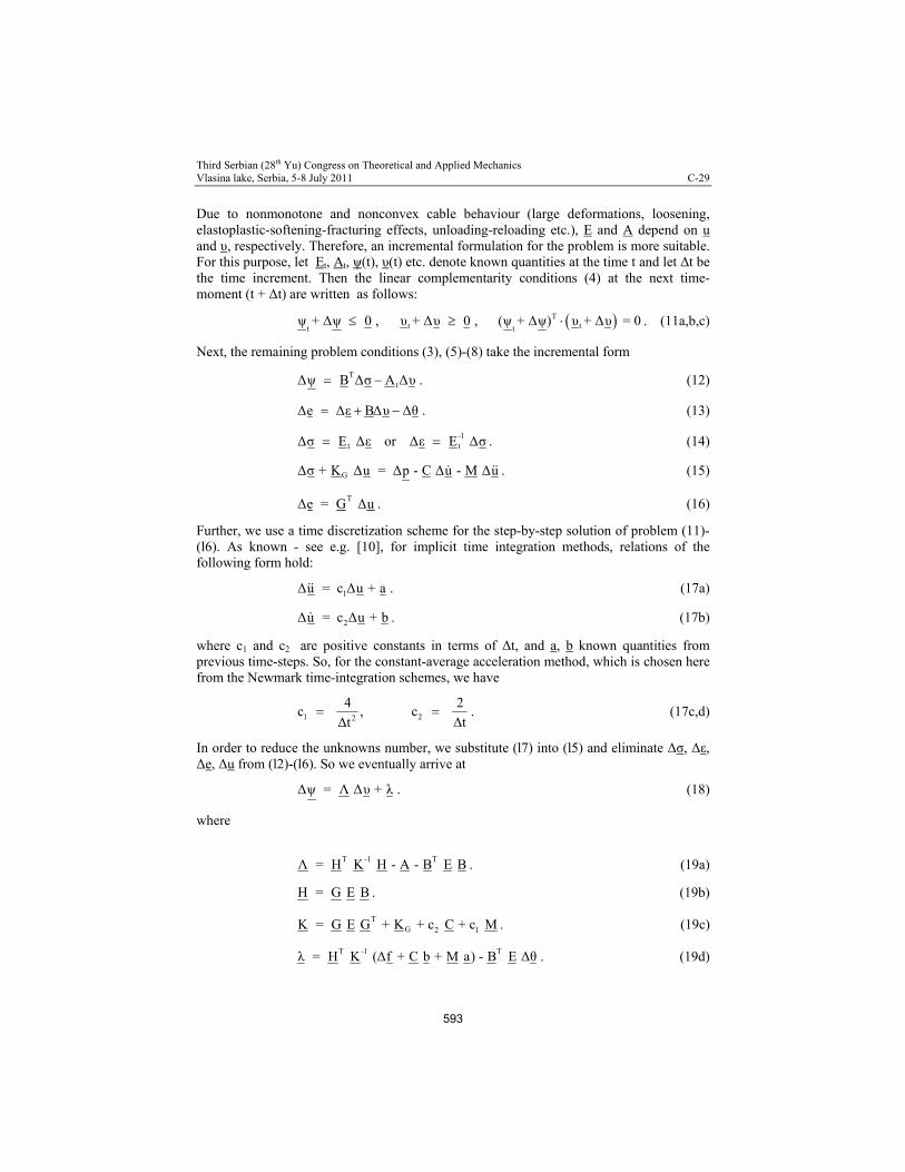
4. Numerical Example The 6-storey framing system of reinforced concrete class C16/20 in Fig. 1, with L = 6 m and h = 4 m, was initially designed and constructed without cable-braces. The beams are of rectangular section 30/75 (width/height, in cm) for the floors i=1,2,3,4, section 25/60 for the floors i=5,6, and have a total vertical distributed load 50 kN/m (each beam). The columns have section dimensions, in cm: 35/50 for the i =1,2 floors, 30/35 for the i = 3,4 floors, and 25/30 for the i = 5,6 floors. Due to environmental actions, corrosion and cracking has been taken place. This had caused a reduction for the section inertia moments, which is estimated [11] to be 10% for the columns and 50% for the beams. So it was necessary for the system to be strengthened. Because of architectural reasons, the cable-braces system shown in Fig. 1 has been applied, and not the usual X-braces [1]. The cable elements, of steel class S400, have a unilateral behaviour depicted in Fig. 2, with yield strain ε y = 0.2 %, fracture strain ε f = 2 % , yield stress σ y = 34.78 kN/cm2, and elasticity modulus Ec = 200 GPa. The branch OA is a 2-nd degree parabola with an horizontal tangent at point A. The system is subjected to the horizontal ground seismic excitation:
-2tg ox (t) = x e sin(4πt) . (20)
where xο = 0.025 m. The graphic representation of xg(t) is shown in Fig. 3. The corresponding maximum seismic ground acceleration is 0.32 g, where g = 9.81 m/sec2 is the gravity acceleration. Further, for comparison reasons, we introduce the comparison coefficients
c
f
Qc =
Q. (21)
where Q is the absolutely maximum value which takes a response quantity during the seismic excitation. Index (c) is for the cable-braced system and index (f) for the free (i.e. without cables) system. Some representative results, obtained by applying the numerical method developed in previous sections, are shown in Table 1. Two cases of cross-sectional area of cables are considered: a) Fc = 3.8 cm2, b) Fc = 7.4 cm2. These results concern on the one hand the comparison coefficients cs for the floor shear forces and cd for the floor horizontal displacements, and on the other hand the stress si [kN/cm2] and the percentage [%] permanent plastic deformation di for the i-th cable element (i = 1,...,6).
594

Third Serbian (28th Yu) Congress on Theoretical and Applied Mechanics Vlasina lake, Serbia, 5-8 July 2011 C-29
Figure 1: Numerical example: The cable-braced 6-storey structural system
Figure 2: Cable-elements constitutive law Figure 3: Seismic horizontal ground
displacement
595

Third Serbian (28th Yu) Congress on Theoretical and Applied Mechanics Vlasina lake, Serbia, 5-8 July 2011 C-29
Table 1. Some results for the numerical example.
Comparison coefficients Cable-Element
Floor cs
(Shear Force)
cd
(Displ. Horiz.)
max si
[kN/cm2]
di
[%]
(0) (1) (2) (3) (4)
1 a 0.921 1.001 17.84 0.128 b 0.884 1.007 17.38 0.107
2 a 0.984 0.963 12.37 0.078 b 0.981 0.945 12.24 0.068
3 a 0.971 1.004 19.63 0.147 b 0.948 1.011 18.01 0.118
4 a 0.971 0.968 15.63 0.108 b 0.982 1.103 15.07 0.091
5 a 1.123 1.171 18.17 0.137 b 1.237 1.378 17.88 0.118
6 a 0.848 1.357 34.78 0.374 b 0.837 1.617 34.78 0.238
As the table values of columns (1) and (2) show, the most influenced floors due to cable behaviour are the two higher ones. So, in the 5th floor the shear floor force increases about 24 % and the displacement about 38 % for case b) with Fc = 7.4 cm2. In the 6th floor it is appeared a decrease about 15 % for the shear force and an increase about 62 % for the displacement. These results can be explained by energy considerations on the basis of the values on columns (3) and (4). Indeed, the cable in the 6th floor has been plastified. Therefore the seismic energy absorbed by it until plastification has returned partially to the frame system. Such effects can be of impact type when cable-elements are fractured, and so the change of response values for the frame can be ocurred in a sudden and pounding way. Moreover, the 6th floor is influenced by the unilateral behaviour of the 6th cable alone. On the contrary, each of the lower floor beams is affected by the combined action of two cables at the same time, and so it is subjected to actions similar to those caused by X-braces. The latter have merely a bilateral character instead of a purely unilateral one. As regards the response of the lower floors, we remark from the table values that as long as the cable remain in the elastic or the early elastoplastic range of their behaviour, i.e. without fracturing, the braced structure appears a reduced response in comparison to that one of the free structure. This fact concerns especially the shear forces in the floors 14, where the corresponding coefficients are about 0.90.
596

Third Serbian (28th Yu) Congress on Theoretical and Applied Mechanics Vlasina lake, Serbia, 5-8 July 2011 C-29
5. Concluding remarks An incremental approach has been herein presented, by which the unilateral dynamic problem of the seismic analysis of cable-braced reinforced concrete structures can be treated numerically. This approach takes into account the unilateral behaviour of cable elements and leads to a linear complementarity problem, in each time increment, with a reduced number of problem unknowns. The numerical realization is obtained by available computer codes of the finite element method, of step-by-step time integration schemes and of mathematical programming (optimization) algorithmes. Moreover, as it has been verified in an example, the herein developed approach can treat in a realistic way the seismic problem of cable-braced reinforced concrete structures in civil engineering praxis.Paper could be divided into sections and subsections.
References
[1] Chopra, A.K.: Dynamics of Structures: Theory and Applications to Earthquake Engineering, Pearson Prentice
Hall, New York, (2007). [2] Newmark, N.M. & E. Rosenblueth.: Fundamentals of Earthquake Engineering. PrenticeHall,Inc, Englewood
Cliffs, N.J., (1971). [3] Panagiotopoulos, P.D.: Stress-Unilateral analysis of discretized cable and membrane structure in the
presence of large displacements. Ingenieur-Archiv, vol. 44, 291-300, (1975). [4] Maier, G. & R. Contro.: Energy approach to inelastic cable-structure analysis. J. Enging Mech. Div., Proc.
ASCE, Vol. 101, EM5, 531-547, (1975). [5] Contro, R. & Maier, G. & A. Zavelani.: Inelastic analysis of suspension structures by nonlinear
programming. Computer Meth. Appl. Mech. Enging, 5, l27-l43, (1975). [6] Maier, G.: Incremental plastic analysis in the presence of large displacements and physical instabilizing
effects. Int. J. Solids Struct. 7, 345–372 (1971). [7] Panagiotopoulos, P.D.: Hemivariational Inequalities. Applications in Mechanics and Engineering. Springer-
Verlag, Berlin, New York, (1993). [8] Panagiotopoulos, P.D.: Non-convex Energy Functions. Hemivariational Inequalities and Substationarity
principles. Acta Mechanica, 48, 111-130, (1983). [9] Liolios, A.A.: A Linear Complementarity Approach for the Non-convex Seismic Frictional Interaction
between Adjacent Structures under Instabilizing Effects. Journal of Global Optimization, vol. 17, no. 1-4, pp. 259-266, (2000).
[10] Weaver, W.Jr. & P.R. Johnston.: Structural dynamics by finite elements. Prentice Hall, Inc, Englewood Cliffs, N.J. (1987).
[11] Pauley T. and Priestley, M.J.N.: Seismic design of reinforced concrete and masonry buildings. Wiley, New York, (1992).
[12] Nitsiotas, G. (1971). Die Berechnung statisch unbestimmter Tragwerke mit einseitigen Bindungen, Ingenieur-Archiv, vol. 41, S. 46-60.
[13] Maier, G., 1973. Mathematical programming methods in structural analysis. In:Brebbia, C. & H. Tottenham (eds.), Variational methods in engineering, Proc. Int. Conf. Southampton University Press, Southampton, Vol. 2, 8/1-8/32.
[14] Zienkiewicz, O.C. & R.L. Taylor, 1989. The finite element method, 4th edition. Mc GrawHill, New York-London .
597

Third Serbian (28th Yu) Congress on Theoretical and Applied Mechanics Vlasina lake, Serbia, 5-8 July 2011 C-30
STRUCTURAL INTEGRITY AND LIFE WITH STEREOMETRIC MACHINE VISION
Jasmina Lozanović Šajić1 1 Faculty of Mechanical Engineering, Innovation Center The University of Belgrade, Kraljice Marije 16, 11120 Belgrade 35 e-mail: [email protected]
Abstract. This paper presents a mobile system that is used to prevent failure of structures. Beginning of the research involved a review of technical measurement system with two cameras – stereometric measurement and machine vision. Fracture mechanics is theoretical number of possible solutions of problems of cracks development approach for assessing structural integrity. There are numerous examples where the rating integrity is used very successfully, but there are still opportunities for new methods of achieving greater efficiency and further cost reduction engineering construction and service.
1. Introduction Machine Vision systems are systems for video processing in industrial conditions where the most common use of these system for product quality control, automatic control of robotic systems, determining the number of people in place frequented, to monitor object in systems for monitoring traffic in biomedical engineering, while in this paper an stereometric system used within an expert system for structural integrity assessment. The term Machine Vision among other things, we mean digitization, analysis and various ways of handling the image (video) which is covered by concept of processing image.
Figure 1. Video cameras "Aramis" with the tested sample at the centre [1]
There are two functionally different methods used for automated control area, this puts an emphasis on surface recording, it will result in this paper used recording surface cracks using stereometric methods:
1. Error detection of uniform structure surface (scratches, marks, holes, etc.) 2. Error detection in the copies preserved in relation to a reference model
598

Third Serbian (28th Yu) Congress on Theoretical and Applied Mechanics Vlasina lake, Serbia, 5-8 July 2011 C-30
Namely, recording with two video cameras were evaluated as suitable contactless method, to obtain information about behavior of the structures during operations. The surface components can spray a contrasting color (black or white background), which are discretized by computer program such as a fingerprint in a unique discretized record of surface. When the construction is loaded, a displacement of points, are saved. This method helps to better understand material and component behavior and is ideally suited to monitor experiments with high temporal and local resolution. This is a non-contact and material independent measuring system providing, for static or dynamically loaded test objects, accurate: 3D surface coordinates, displacements and velocities, Surface strain values (major and minor strain, thickness reduction), Strain rates This is the ideal solution for: Determination of material properties (R- and N-values, FLC, Young's Modulus, etc...), Component analysis (crash tests, vibration analysis, durability studies, etc...), Verification of Finite Element Analysis. It is ideally suited to measure, with high temporal and local resolution as well as with a high accuracy, three-dimensional deformation and strain in real components and material specimens. For static or dynamically loaded specimens and components, ARAMIS allows for non-contact and material independent determination of 3D coordinates and 3D displacements, 3D speeds and accelerations, Plane strain tensor and plane strain rate, Material characteristics. By this method is possible to obtain a complete picture of deformation of structural components by the real time with the change of the spatial components of deformations . Coordinates of selected points of the network are changing due shifting these points, caused by increasing load. , monitoring of coordinates is possible by using a complex mathematical apparatus, which contains expressions to determine the strain components, and expressions that are used for assessing structural integrity. The aim was stereometric measurement applications application in the analysis if structures under the influence of external loads. Fracture mechanics is theoretical number of possible solutions of problems of crack development approach for assessing structural integrity. There are numerous examples where integrity assessment is used very successfully, but there are still possibilities of new method to achieve greater efficiency and further cost reduction engineering, construction and service construction. A special problem is the structure composed of several different materials. Basis for stereometric measuring are two examples of transient crack and an example of surface cracks in tubes for fracture mechanics testing.
2. Setting up the experiment and development of numerical models
In the thesis [2] made the following test tubes: - experimental (in laboratory for mechanical testing) - stereometric measurements (monitor the deformation in real time during
mechanical load) - numeric (using licensed software for calculation of FEM), and - analytical (FAD and CDF diagrams)
599

Third Serbian (28th Yu) Congress on Theoretical and Applied Mechanics Vlasina lake, Serbia, 5-8 July 2011 C-30
Figure 2. Model for numerical analysis.
In Figure 3, the data of distribution of equivalent von Mises’s stress obtained for model with crack and fine mesh finite elements. The results obtained are preliminary, because the tensile properties of materials that make up circuit modeled using a simplidied bilinear strength curves.
Figure 3. Distribution of von Mises’s stress on models with a crack and fine mesh.
3. Results obtained by stereometric measurement Stereometric measurement was performed on two specimens, because strength testing machine and get better results stereometric results steremetric stereometric measurement, the specimens have gone to further processing and finishing before the test. The test were concluded welded joints of low-carbon steel increased strength X60, which is designed for longitudinally welded pipes exposed to high pressure vessels. Chemical compositions and mechanical properties of X60 steel are given in Table 1 and Table 2, consequently.
600

Third Serbian (28th Yu) Congress on Theoretical and Applied Mechanics Vlasina lake, Serbia, 5-8 July 2011 C-30
Figure 3. Tensioning specimen in testing machine with controlled growth force and stereometric monitoring crack
growth.
Table 1. Chemical Compositions, X60
mass. % C Mn P S Co V Nb
0.12 0.33 0.020 0.010 0.35 0.045 0.056
Table 2. Mechanical Properties, X60
448 596 22.7 55.6 76
Plate specimen with initial crack in the test specimen material resistance to fracture and define standards. Initial crack the test specimen with K welded joint were conducted electro-erosion and dynamically changing load. The study was concluded on electro-mechanical testing machine, and was used stereometric method.
Figure 4. Stereometric measurement of specimen with initial crack.
601
Third Serbian (28th Yu) Congress on Theoretical and Applied Mechanics Vlasina lake, Serbia, 5-8 July 2011 C-30
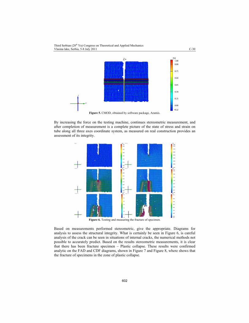
Figure 5. CMOD, obtained by software package, Aramis.
By increasing the force on the testing machine, continues stereometric measurement, and after completion of measurement is a complete picture of the state of stress and strain on tube along all three axes coordinate system, as measured on real construction provides an assessment of its integrity.
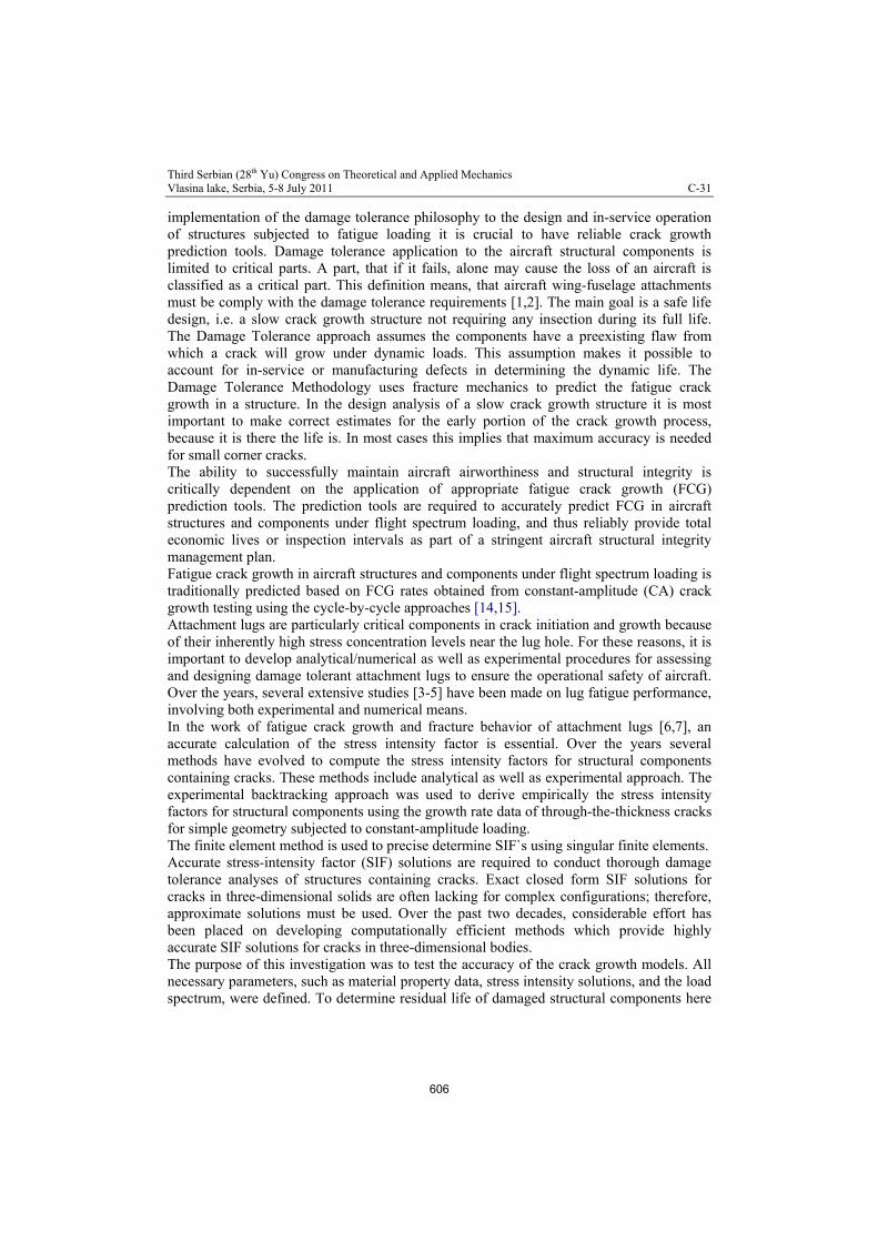
Figure 6. Testing and measuring the fracture of specimen.
Based on measurements performed stereometric, give the appropriate. Diagrams for analysis to assess the structural integrity. What is certainly be seen in Figure 6, is careful analysis of the crack can be seen in situations of internal cracks, the numerical methods not possible to accurately predict. Based on the results stereometric measurements, it is clear that there has been fracture specimen – Plastic collapse. These results were confirmed analytic on the FAD and CDF diagrams, shown in Figure 7 and Figure 8, where shows that the fracture of specimens in the zone of plastic collapse.
602

Third Serbian (28th Yu) Congress on Theoretical and Applied Mechanics Vlasina lake, Serbia, 5-8 July 2011 C-30
Figure 7. FAD diagram for specimen
Figure 8. CDF diagram for specimen
Figure 8. Fracture specimen
603

Third Serbian (28th Yu) Congress on Theoretical and Applied Mechanics Vlasina lake, Serbia, 5-8 July 2011 C-30
4. Conclusion The research of this study showed good agreement between experimental, analytical and numerical analysis of deformation behavior of structural components with different configurations and different ways of cracking loads. Paramerers of fracture mechanics and limit load were calculated analytically and numerically, and experimentally verified aquipment measuring displacement and strain at the surface were studied components. Comparisons between analytical and numerical results on surface and corresponding experimental results have shown that it is possible to trace the behavior structural components of the cracked and assume the existence, location size and development of internal cracks. The agreement between analytical, numerical and experimental results is good for surface cracks. Less agreement of numerical and experimental results are in internal cracks because they cannot be assumed true, the reason lies in the structure of material, as in the case welded jointsm, which are usually not taken into account in numerical modeling base material, but is taken into account in welded joints when differences in strength exceed some percentage (eg SINTAP- Structural Integrity Assessment Procedures for European Industry-is more than 10%). Results showed that data obtained with stereometric method correspond well with numerical and analytical results which gives us justification for introducing such expert system.
References [1] AramisGOMmbH, http://www.gom.com [2] Jaсмина Лозановић, Аутоматизација стереометријског мерења приликом одређивања напонског стања око врха прслине и процена интегритета конструкције, докторска дисертација, одрањена 02.06.2009., на Машинском факултету Универзитета у Београду. [3] N. Gubeljak, J. Lozanovic, A. Sedmak, Crack tip strain and CTOD in situ measurement, First Serbian (26th YU) Congress on Theoretical and Applied Mechanics, Kopaonik, Serbia, April, 2007. p.p. 1103-1108. [4] Jasmina Lozanović, Aleksandar Sedmak, Nenad Gubeljak, Measurement of Strain Using Stereometry, TEHNIČKI VJESNIK - TECHNICAL GAZETTE, Tehnički vjesnik, Vol.16. No.4 Prosinac 2009, p.p. 93-99
604

Third Serbian (28th Yu) Congress on Theoretical and Applied Mechanics Vlasina lake, Serbia, 5-8 July 2011 C-31
RESIDUAL LIFE ESTIMATION OF DAMAGED STRUCTURAL COMPONENTS
USING LOW-CYCLE FATIGUE PROPERTIES
1Maksimovic S., 2Vasovic I., 3Maksimović M., 1Đurić M. 1 Military Technical Institute- Department of Aeronautics Ratka Resanovica 1, Belgrade, Serbia e-mail: [email protected] 2 Institut Goša, Milana Rakica 35, Belgrade, Serbia e-mail: [email protected] 3 Water Supply, Belgrade, Serbia e-mail: [email protected]
Abstract. The goal of this paper is the establishment of computation method for the evaluation of the residual life of structural elements in the presence of initial damage which appears in the form of cracks. Therefore in this paper computation method for the evaluation of the residual life of structural elements with initial damage subjected to cyclic loading of constant amplitude load spectrum are presented. Computational methods for the evaluation of the residual life of structural elements with initial damage basically rely on crack propagation analysis. In this investigation for crack propagation analysis Strain Energy Density (SED) method will be used. This method uses the low-cycle fatigue (LCF) properties of the material, which are also being used for the lifetime evaluation until the occurrence of initial damage. Therefore experimentally obtained dynamic properties of the material such as Paris` constants are not required when this approch is concerned. The complete computation procedure for the crack propagation analysis using low-cycle fatigue material properties is illustrated with the damaged structural elements. To determine analytic expressions for stress intensity factors (SIF) singular finite elements are used. Results of numerical simulation for crack propagation based on strain density method have been compared with own experimental results.
Key words: Fatigue, residual life, damaged structural elements, aircraft attachment lugs, strain energy density method, low-cycle fatigue properties, finite elements
1. Introduction Methods for design against fatigue failure are under constant improvement. In order to optimize constructions the designer is often forced to use the properties of the materials as efficiently as possible. One way to improve the fatigue life predictions may be to use relations between crack growth rate and the stress intensity factor range. These are fairly well established for constant amplitude loading, at least for common specimen geometries. Loading histories in engineering structures do however often exhibit varying amplitudes. For such cases the prediction capacity is markedly lower. Ideally, the crack advance under varying amplitude should be possible to predict using experimental data from constant amplitude testing. Numerous investigations address this problem but so far without reaching any total success. Design based on damage tolerance criteria often deals with notched components giving rise to localized stress concentrations which, in brittle materials, may generate a crack leading to catastrophic failure or to a shortening of the assessed structural life. For a successful
605
Third Serbian (28th Yu) Congress on Theoretical and Applied Mechanics Vlasina lake, Serbia, 5-8 July 2011 C-31
implementation of the damage tolerance philosophy to the design and in-service operation of structures subjected to fatigue loading it is crucial to have reliable crack growth prediction tools. Damage tolerance application to the aircraft structural components is limited to critical parts. A part, that if it fails, alone may cause the loss of an aircraft is classified as a critical part. This definition means, that aircraft wing-fuselage attachments must be comply with the damage tolerance requirements [1,2]. The main goal is a safe life design, i.e. a slow crack growth structure not requiring any insection during its full life. The Damage Tolerance approach assumes the components have a preexisting flaw from which a crack will grow under dynamic loads. This assumption makes it possible to account for in-service or manufacturing defects in determining the dynamic life. The Damage Tolerance Methodology uses fracture mechanics to predict the fatigue crack growth in a structure. In the design analysis of a slow crack growth structure it is most important to make correct estimates for the early portion of the crack growth process, because it is there the life is. In most cases this implies that maximum accuracy is needed for small corner cracks. The ability to successfully maintain aircraft airworthiness and structural integrity is critically dependent on the application of appropriate fatigue crack growth (FCG) prediction tools. The prediction tools are required to accurately predict FCG in aircraft structures and components under flight spectrum loading, and thus reliably provide total economic lives or inspection intervals as part of a stringent aircraft structural integrity management plan. Fatigue crack growth in aircraft structures and components under flight spectrum loading is traditionally predicted based on FCG rates obtained from constant-amplitude (CA) crack growth testing using the cycle-by-cycle approaches [14,15]. Attachment lugs are particularly critical components in crack initiation and growth because of their inherently high stress concentration levels near the lug hole. For these reasons, it is important to develop analytical/numerical as well as experimental procedures for assessing and designing damage tolerant attachment lugs to ensure the operational safety of aircraft. Over the years, several extensive studies [3-5] have been made on lug fatigue performance, involving both experimental and numerical means. In the work of fatigue crack growth and fracture behavior of attachment lugs [6,7], an accurate calculation of the stress intensity factor is essential. Over the years several methods have evolved to compute the stress intensity factors for structural components containing cracks. These methods include analytical as well as experimental approach. The experimental backtracking approach was used to derive empirically the stress intensity factors for structural components using the growth rate data of through-the-thickness cracks for simple geometry subjected to constant-amplitude loading. The finite element method is used to precise determine SIF`s using singular finite elements. Accurate stress-intensity factor (SIF) solutions are required to conduct thorough damage tolerance analyses of structures containing cracks. Exact closed form SIF solutions for cracks in three-dimensional solids are often lacking for complex configurations; therefore, approximate solutions must be used. Over the past two decades, considerable effort has been placed on developing computationally efficient methods which provide highly accurate SIF solutions for cracks in three-dimensional bodies. The purpose of this investigation was to test the accuracy of the crack growth models. All necessary parameters, such as material property data, stress intensity solutions, and the load spectrum, were defined. To determine residual life of damaged structural components here
606
Third Serbian (28th Yu) Congress on Theoretical and Applied Mechanics Vlasina lake, Serbia, 5-8 July 2011 C-31
are used two crack growth methods: conventional Forman`s crack growth method and crack growth model based on the strain energy density method. The last metod uses the low cycle fatigue properties in the crack growth model.
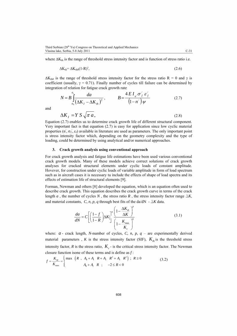
2. Crack growth model based on Strain Energy Density Method In this work fatigue crack growth method based on energy concept is considered and then it is necessary to determine the energy absorbed till failure. This energy can be calculated by using cyclic stress-strain curve. Function between stress and strain, as recommended by Ramberg-Osgood provides good description of elastic-plastic behavior of material, and may be expressed as
/
1
/22
n
kE
. (2.1)
where E is the modulus of elasticity, /2 is strain amplitude and /2 is stress amplitude. Equation (2.1) enables the calculation of the stress-strain distribution by knowing low cyclic fatigue properties. As a result the energy absorbed till failure become [10,11]
//
/1
4ffc
nW
(2.2)
where f/ is cyclic yield strength and f
/ - fatigue ductility coefficient. Given the fact that strain energy density method is considered, the energy absorbed till failure must be determined after the energy concept is based on the following fact: The energy absorbed per unit growth of crack is equal to the plastic energy dissipated within the process zone per cycle. This energy concept is expressed by
Wc a = p, (2.3)
where Wc is energy absorbed till failure, p- the plastic energy and a - the crack length. In equation (2.3) it is necessary just to determine the plastic energy dissipated in the process zone p. By integration of equation for the cyclic plastic strain energy density in the units of Joule per cycle per unit volume 10 from zero to the length of the process zone ahead of crack tip d* it is possible to determine the plastic energy dissipated in the process zone p. After integration relation of the plastic energy dissipated in the process zone becomes
/
2
/
/
1
1
n
Ip IE
K
n
n
(2.4)
where KI is the range of stress intensity factor, - constant depending on the strain hardening exponent n/, In
/ - the non-dimensional parameter depending on n/. Fatigue crack growth rate can be obtained by substituting Eq. (2.2) and Eq. (2.4) in Eq. (2.3)
2
//
/
/4
1thI
ffn
KKIE
n
dN
da
, (2.5)
607
Third Serbian (28th Yu) Congress on Theoretical and Applied Mechanics Vlasina lake, Serbia, 5-8 July 2011 C-31
where Kth is the range of threshold stress intensity factor and is function of stress ratio i.e.
Kth= Kth0(1-R), (2.6) Kth0 is the range of threshold stress intensity factor for the stress ratio R = 0 and is coefficient (usually, = 0.71). Finally number of cycles till failure can be determined by integration of relation for fatigue crack growth rate
ca
a thI KK
daBN
0
2,
/
//
1
4 /
n
IEB
ffn
(2.7)
and
,aSYK I (2.8)
Equation (2.7) enables us to determine crack growth life of different structural component. Very important fact is that equation (2.7) is easy for application since low cyclic material properties (n/, f
/, f) available in literature are used as parameters. The only important point is stress intensity factor which, depending on the geometry complexity and the type of loading, could be determined by using analytical and/or numerical approaches.
3. Crack growth analysis using conventional approach
For crack growth analysis and fatigue life estimations have been used various conventional crack growth models. Many of these models achieve correct solutions of crack growth analyses for cracked structural elements under cyclic loads of constant amplitude. Hovever, for construction under cyclic loads of variable amplitude in form of load spectrum such as in aircraft cases it is necessary tu include the effects of shape of load spectra and its effects of estimation life of structural elements [9].
Forman, Newman and others [8] developed the equation, which is an equation often used to describe crack growth. This equation describes the crack growth curve in terms of the crack length a , the number of cycles N , the stress ratio R , the stress intensity factor range DK,
and material constants, C, n, p, q through best fits of the da/dN - DK data.
max
11
11
p
thn
q
c
Kda f K
C KdN R K
K
(3.1)
where: - crack length, N-number of cycles, C, n, p, q – are experimentally derived
material parameters , K is the stress intensity factor (SIF), is the threshold stress
intensity factor, R is the stress ratio, - is the critical stress intensity factor. The Newman
closure function isone of these terms and is define as f :
a
thK
cK
2 30 1 2
; 2
A
3
ma 0 1
max , ; 0
0
R A A R R A R RKf
K A A R R
x
op (3.2)
608

Third Serbian (28th Yu) Congress on Theoretical and Applied Mechanics Vlasina lake, Serbia, 5-8 July 2011 C-31
and the coefficients are given by: 1
2 max0
0
(0.825 34 0.05 ) cos(2
SA
1 0(0.415 0.071 ) /msxA S
2 0 11A A A 3A
3 0 12 1A A A where: - is the plane stress/strain constraint factor, (max/0) is the ratio of maximum stress to the flow stress. The threshold stress intensity factor range is calculated by the following empirical equation:
1 (1 )2
0
1/
1 (1 )(1 )
thC R
th tho
a fK K
a A R
(3.3)
Relation (3.1) represents one general crack growth models based on conventional approach. This relation can be transformed to conventional Forman`s crack growth model5. In region III rapid and unstable crack growth occurs, so Forman at al. Proposed equation for region III as well as for region II [9]
1
n
C
C Kda
dN R K K
(3.4)
where KC is the fracture toughness. Forman`s equation has been developed to model of unstable crack growth domain (III).
4. Stress intensity factor solution of cracked lugs
4.1 Damaged attachment lug with initial crack through the thickness
In this section are given relations for stress intensity factor with crack through the thickness In general geometry of notched structural components and loading is too complex for the stress intensity factor (SIF) to be solved analytically. The SIF calculation is further complicated because it is a function of the position along the crack front, crack size and shape, type loading and geometry of the structure. In this work analytic and FEM were used to perform linear fracture mechanics analysis of the pin-lug assembly. Analytic results are obtained using relations derived in this paper. Good agreement between finite element and analytic results is obtained. It is very important because we can to use analytic derived expresions in crack growth analyses. Lugs are essential components of an aircraft for which proof of damage tolerance has to be undertaken. Since the literature does not contain the stress intensity solution for lugs which are required for proof of damage tolerance, the problem posed in the following investigation are: selection of a suitable method of determining othe SIF, determination of SIF as a function of crack length for various form of lug and setting up a complete formula for calculation of the SIF for lug, allowing essential parameters. The stress intensity factors are the key parameters to estimate the characteristic
609
Third Serbian (28th Yu) Congress on Theoretical and Applied Mechanics Vlasina lake, Serbia, 5-8 July 2011 C-31
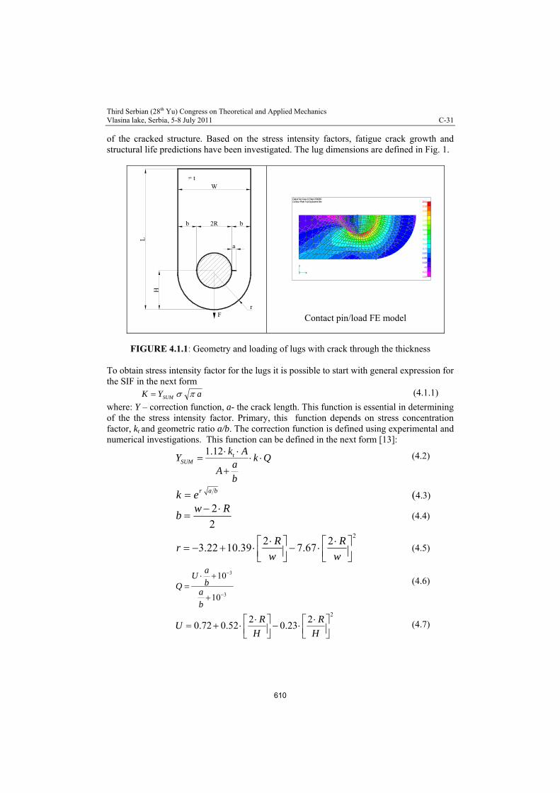
of the cracked structure. Based on the stress intensity factors, fatigue crack growth and structural life predictions have been investigated. The lug dimensions are defined in Fig. 1.
L
H
W
a
F
= t
2R bb
r
Contact pin/load FE model
X
Y
Z
29.01
27.28
FIGURE 4.1.1: Geometry and loading of lugs with crack through the thickness
To obtain stress intensity factor for the lugs it is possible to start with general expression for the SIF in the next form aYK SUM (4.1.1)
where: Y – correction function, a- the crack length. This function is essential in determining of the the stress intensity factor. Primary, this function depends on stress concentration factor, kt and geometric ratio a/b. The correction function is defined using experimental and numerical investigations. This function can be defined in the next form [13]:
1.12 tSUM
k AY
aA
b
k Q (4.2)
r a bk e (4.3) 2
2
wb
R (4.4)
22 2
3.22 10.39 7.67R R
rw w
(4.5)
3
3
10
10
aU
bQab
(4.6)
22 2
0.72 0.52 0.23R R
UH H
(4.7)
25.55
23.82
22.09
20.36
18.63
16.9
15.17
13.45
11.72
9.987
8.258
6.529
4.8
3.071
1.342
Output Set: Case 12 Step 0.500000Contour: Plate Top Equivalent Stre
610

Third Serbian (28th Yu) Congress on Theoretical and Applied Mechanics Vlasina lake, Serbia, 5-8 July 2011 C-31
1.895 1
0.026a
bA e (4.8)
The stress concentration factor kt is very important in calculation of correction function, eq. 4.2. In this investigation. A contact finite element stress analysis was used to analyze the load transfer between the pin and lug.
4.2 Damaged attachment Lug with semi-elliptic surface crack
Here is considered the stress intensity factors for cracked lug with the semi-elliptic surface crack as shown in Fig. 4.2.1.
Ro
Ri
A t
2b
a
FIGURE 4.2.1 Lug with semi-elliptic surface crack
As start point for determination of stress intensity factor of attachment lug with semi-elliptic surface crack will be used Lukaš`s model [16,17]. Lukaš is considered problem of determination of SIF to plate with surface crack within zone of stress concentration. This approached is extended to the attachment lugs with semi-elliptic surface crack. By using this approach here are defined analytic expressions for determination of SIF`s at the points А and B to lug with semi-elliptic surface crack as shown in Fig. 4.2.1, in the next form:
A A tK F k a (4.3.1)
AA A,0
DF F
a (4.3.2)
611

Third Serbian (28th Yu) Congress on Theoretical and Applied Mechanics Vlasina lake, Serbia, 5-8 July 2011 C-31
A,0
2
a1.13 0.09
abF ,
a bE
b
0 1 (4.3.3)
a
aAD a d 1 e
(4.3.4)
2t
da
k 1
4.3.5)
B B tK F k a (4.3.6)
BB B,0
DF F
a (4.3.7)
a
4aBD a 4d 1 e
(4.3.8)
B,0
2
a1.243 0.099
abF
a bEb
(4.3.9)
Горњи аналитички изрази за ФИН код ушке са елиптичном прскотином се могу користити како за прорачун чврстоће ушки са аспекта “статичке” механике лома тако и за процену преосталог века коришћењем различитих закона ширења прскотине. 5. Numerical validation To illustrate computation procedures in damage tolerance analysis and residual life estimations of damged structural components here are numerical examples included. 5.1 Life estimation of damaged structural elements Subject of this analyses are cracked aircraft lugs under cyclic load of conctant amplitude end spectra. For that purpose conventional Forman crack growth model and crack growth model based on strain energy density method are used. Material of lugs is Aluminum alloy 7075 T7351 with the next material properties: m=432 N/mm2 Tensile strength of material 02=334 N/mm2 KIC=2225 [N/mm3/2] Dynamic material properties (Forman`s constants): CF=3* 10-7, nF=2.39. Cyclic material properties: f
/=613 МПа, f/=0.35 , n/=0.121.
612

Third Serbian (28th Yu) Congress on Theoretical and Applied Mechanics Vlasina lake, Serbia, 5-8 July 2011 C-31
The stress intensity factors (SIF`s) of cracked lugs are determined for nominal stress levels: g = max=98.1 N/mm2 and min=9.81 N/mm2. These stresses are determined in net cross-section of lug. The corresponding forces of lugs are defined as, Fmax= g (w-2R) t = 63716 N and Fmin= 6371.16 N, that are loaded of lugs. For stress analyses contact pin/lug finite element model is used. For cracked lugs defined in Table 5.1, with initial cracks a0, SIF`s are determined using finite elements, Table 5.2. To obtain high-quality results of SIF`s cracked lugs are modeled by singular finite elements around crack tip.
160
44.4
R20
R41
83.3
t = 15 mm
a
F = 6371.6 daN
Fig 5.1: Geometry of cracked lug 2
Fig. 5.2. Finite Element Model of cracked lug with stress distribution
Table 5.1: Geometric parameters of lugs [13]
Dimensions [mm] Lug No. 2R W H L t 2 6 7
40 40 40
83.3 83.3 83.3
44.4 57.1 33.3
160 160 160
15 15 15
The stress intensity factors of cracked lugs are calculated under stress level: g = max=98.1 N/mm2, or corresponding axial force, Fmax= g (w-2R) t = 63716 N. In present finite element analysis of cracked lug is modeled with special singular quarter-point six-node finite elements around crack tip, Fig. 5.2. The load the model, a concentrated force, Fmax, was applied at the center of the pin and reacted at the other and of the lug. Spring elements were used to connect the pin and lug at each pairs of nodes having identical nodal coordinates all around the periphery. The area of contact was determined iteratively by assigning a very high stiffness to spring elements which were in compression and very low stiffness (essentially zero) to spring elements which were in tension. The stress intensity factors of lugs, analytic and finite elements, for through-the-thickness cracks are shown in Table 5.2. Analytic results are obtained using relations from previous sections, eq. (4.1.1).
613

Third Serbian (28th Yu) Congress on Theoretical and Applied Mechanics Vlasina lake, Serbia, 5-8 July 2011 C-31
Table 5.2: Comparisons analytic with FEM results of SIF
Lug No.
mma MKEIK max
.max
ANALIK
2 5.00 68.784 65.621 6 5.33 68.124 70.246 7 4.16 94.72 93.64
From above Table 5.2 is evident good agreement between analytic and finite element results for determination of stress intensity factors. Accuracy of SIF`s is very important in precise crack growth analyses and life estimation of cracked lugs. That means that proposed analytic model for determination of SIF`s is adequate in crack growth analyses.In design process is very important to know how any geometric parameters of lug have the effects on fracture mechanics parameters. In Fig. 5.4 are shown dependence SIF, Kmax, and height of head of lug H. In this analysis geometric properties of lugs are given in Table 5.1. From Fig. 5.4 is evident increasing of SIF`s with increasing crack length and reducing with increasing height of lug`s head. In Fig. 5.3 are shown computation and experimental results of cracked lug No. 2 as defined in Fig. 5.1 and Table 5.1. In this computation analysis Forman crack growth model is used. Good agreement between computation and experimental results is obtained. It is evident that computation Forman`s crack growth model is to a small extent conservative for longer crack, Fig. 5.3.
Fig. 5.3 Comparisons computational with experimental crack growth results for lug
No. 2 (H=44.4 mm); kt=2.8
Nf x 103
614
Third Serbian (28th Yu) Congress on Theoretical and Applied Mechanics Vlasina lake, Serbia, 5-8 July 2011 C-31
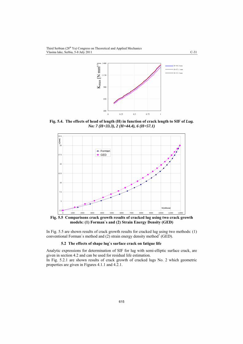
a/b 400
650
900
1 1 50
1 400
0 0.25 0.5 0.75 1
H=44. 4 mm
H=57. 1 mm
H=33. 3 mm
][N
mm
max
K0.
5
Fig. 5.4. The effects of head of length (H) in function of crack length to SIF of Lug. No: 7 (H=33.3), 2 (H=44.4), 6 (H=57.1)
2.5
5
7.5
10
12.5
15
17.5
20
22.5
0 1000 2000 3000 4000 5000 6000 7000 8000 9000 10000 11000 12000
N [ciklusa]
a [
mm
]
FormanGED
Fig. 5.5 Comparisons crack growth results of cracked lug using two crack growth
models: (1) Forman`s and (2) Strain Energy Density (GED) In Fig. 5.5 are shown results of crack growth results for cracked lug using two methods: (1) conventional Forman`s method and (2) strain energy density method7 (GED).
5.2 The effects of shape lug`s surface crack on fatigue life
Analytic expressions for determination of SIF for lug with semi-elliptic surface crack, are given in section 4.2 and can be used for residual life estimation. In Fig. 5.2.1 are shown results of crack growth of cracked lugs No. 2 which geometric properties are given in Figures 4.1.1 and 4.2.1.
615

Third Serbian (28th Yu) Congress on Theoretical and Applied Mechanics Vlasina lake, Serbia, 5-8 July 2011 C-31
b0=2.5
0
1
2
3
4
5
6
7
8
0 2000 4000 6000 8000 10000 12000
N [broj ciklusa]
a [m
m]
Total
Eliptik
Fig. 5.2.1. Comparisons crack growth results of attachment lug with crack through
the thickness and semi-elliptic surface crack
In Figure 5.2.1 is shown the effect of lug`s shape of surface crack on residual fatigue life. As expected reduced life has lug with crack through the thickness (“total”) then lug with semi-elliptic surface crack (“eliptik”).
5. Conclusions This investigation is focused on developing efficient and reliable computation methods for fatigue life estimation of damaged structural components. An special attention has been focused on determination of fracture mechanics parameters of structural components such as stress intensity factors of aircraft cracked lugs. The effects of shape of lug`s surface crack on residual fatigue life is investigation too. Predictions and experimental investigations for fatigue life of an attachment lug under load spectrum were performed. From this investigation followings are concluded: A model for the fatigue crack growth is included which incorporates the low cycle fatigue properties of the material. Comparisons of the predicted crack growth rate using strain energy method method with experimental data and conventional Forman`s model points out the fact that this model could be effective used for residual life estimations The stress intensity factor of cracked lug is well defined by analytical method since there is really minor difference when compared results obtained by singular finite elements. The effects of of shape of attachment lug`s surface crack on residual fatigue life is evident. Acknowledgments The authors would like to thank the Ministry of Science and Technological Development of Serbia for financial support under the project numbers TR 35045 and OI 174001.
616

Third Serbian (28th Yu) Congress on Theoretical and Applied Mechanics Vlasina lake, Serbia, 5-8 July 2011 C-31
References [1] “Airplane Damage Tolerance Requirements”, MIL-A-83444, Air Force Aeronautical
Systems Division, July 1974. [2] Brussat, T.R., Kathiresan, K and Rud, J.L., Damage tolerance assessment lugs,
Engineering Fracture Mechanics, 23, 1067-1084, 1986 [3] Maksimović, S., Fatigue Life Analysis of Aircraft Structural Components, Scientific
Technical Review, 2005. [4] Maksimović K., Nikolić-Stanojević V., Maksimović S., MODELING OF THE
SURFACE CRACKS AND FATIGUE LIFE ESTIMATION, ECF 16, 16th European Conference of Fracture, ECF 16, Alexandroupolis, Grčka, 2006.
[5] Maksimović, S., Boljanović, S, Maksimović, K., Fatigue life prediction of Structural Components under variable amplitude loads, FATIGUE 2002, 8th International Fatigue Congress (IFC8), Stocholm, 2-6. June, 2002.
[6] Antoni, N and Gaisne F., Analytical modeling for static stress analysis of pin-loaded lugs with bush fitting, Applied Mathematical Modeling, 35, 2011, 1-21.
[7] Liu, Y.Y and Lin F.S., A mathematical equation relating low cycle fatigue data to fatigue crack propagation rates. Int. J. Fatigue, Vol. 6 (1984), pp.31-36
[8] Forman, R. G., and Mettu, S. R., “Behavior of Surface and Corner Cracks Subjected to Tensile and Bending Loads in Ti-6Al-4V Alloy,” Fracture Mechanics: Twenty-second Symposium, Vol. 1, ASTM STP 1131, H. A. Ernst, A. Saxena, and D. L., McDowell, eds., American Society for Testing and Materials, Philadelphia, 1992, pp. 519-546.
[9] Forman, R.G., V.E. Kearney and R. M. Engle, Numerical analysis of crack propagation in cyclic loaded structures, J. Bas. Engng. Trans. ASME 89, 459, 1967.
[10] ] Liu S.B and Tan C.L., Boundary element contact mechanics analysis of pin-loaded lugs with single cracks, Engineering Fracture Mechanics, Vol. 48,No.5, 717-725, 1994.
[11] Maksimović, S., Boljanović, S., Fatigue Life Prediction of Structural Components Based on Local Strain and an Energy Crack Growth Models, WSEAS TRANSACTIONS on APPLIED and THEORETICAL MECHANICS, Issue 2, Volume 1, 2006, pp 196-205..
[12] Maksimović, K., Maksimović, S., Analytic approach for determination of fracture mechanics parameters and crack growth analysis of 3-D surface cracked structural elements, Technical Diagnostic, Vol. III, No. 1, 2004.
[13] Maksimović K., Damage tolerance analysis of aircraft constructions under dynamic loading, Master Thesis, Faculty of Mechanical Engineering, 2003.
[14] Ball D, Norwood D, TerMaath S. Joint strike fighter airframe durability and damage tolerance certification. In: Proceedings of the 47th AIAA/ASME/ASCE/AHS/ASC structures, structural dynamics, and materials conference, Newport, Rhode Island, USA; May 2006.
[15] Schijve J. Fatigue of structures and materials in the 20th century and the state of art. Int J Fatigue 2003;25:679–702.
[16] Lukaš, P., Stress intensity factor for small notch-emanated cracks, Engineering Fracture Mechanics, 26 (3), 471-3, 1987.
[17] Wormsen, A., Fjeldstad, A., Harkegard, G., The application of asѕimptotic solutions to a semi-elliptical crack at the root of a notch, Engineering Fracture Mechanics, Vol. 73, 1889-1912, 2006.
617

Third Serbian (28th Yu) Congress on Theoretical and Applied Mechanics Vlasina lake, Serbia, 5-8 July 2011 C-32
NUMERICAL MODELLING OF MASONRY WALLS SUBJECTED
TO LATERAL IN-PLANE LOAD
R. Mandić1, R. Salatić2, Z. Perović3 1 Faculty of Civil Engineering The University of Belgrade, Bulevar kralja Aleksandra 73, 11000 Belgrade e-mail: [email protected] 2 Faculty of Civil Engineering The University of Belgrade, Bulevar kralja Aleksandra 73, 11000 Belgrade e-mail: [email protected] 3 Faculty of Civil Engineering The University of Belgrade, Bulevar kralja Aleksandra 73, 11000 Belgrade e-mail: [email protected]
Abstract. Masonry walls are traditionally used as main vertical structural elements in low rise buildings. The masonry walls are also used as infill in high rise frames, but in this case their presence usually is neglected in the structural design although they significantly modify the structural response especially in the case of seismic loading. Seismic resistance of masonry wall depends on wall geometry, vertical loads and on characteristic of brick-mortar interface connection. The nonlinear response of the connection between unit and mortar represents the most important feature of masonry behaviour which has to be considered in the modelling of masonry. In this paper some results of a numerical finite element study on the monotonic response of masonry panels subjected to lateral loading are given. A comparison between numerical results and experimental data points out the ability of the proposed model to trace the overall shear performances of masonry walls.
1. Introduction Beside the stone, masonry is the oldest building material and it still widely present in building construction. In many existing buildings masonry walls are main vertical bearing elements. In Serbia and surrounding countries the masonry in low rise buildings is extensively used with vertical and horizontal belt beams. In high rise reinforced concrete frames the masonry infill are treated as a secondary (non-structural) element. However, they significantly influence the response of framed structures, particularly in the case of earthquake loading, by increasing the initial stiffness and changing the dynamic properties of the whole system by forming the mechanism with large dissipation energy in the case of reversed dynamic response. The full understanding of behavior of masonry walls under lateral load is important from the point of view of seismic assessment and retrofitting of existing buildings or the construction of new ones. For the walls subjected to in-plane lateral loading the cracking of mortar joints starts for very low levels of lateral loading. This generate non-linear response from the very
618
Third Serbian (28th Yu) Congress on Theoretical and Applied Mechanics Vlasina lake, Serbia, 5-8 July 2011 C-32
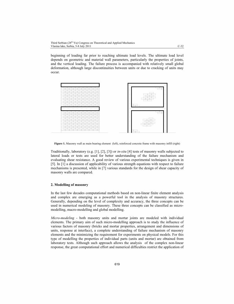
beginning of loading far prior to reaching ultimate load levels. The ultimate load level depends on geometric and material wall parameters, particularly the properties of joints, and the vertical loading. The failure process is accompanied with relatively small global deformation, although large discontinuities between units or due to cracking of units may occur.
Figure 1. Masonry wall as main bearing element (left), reinforced concrete frame with masonry infill (right)
Traditionally, laboratory (e.g. [1], [2], [3]) or in-situ [4] tests of masonry walls subjected to lateral loads or tests are used for better understanding of the failure mechanism and evaluating shear resistance. A good review of various experimental techniques is given in [5]. In [1] a discussion of applicability of various strength equations with respect to failure mechanisms is presented, while in [7] various standards for the design of shear capacity of masonry walls are compared. 2. Modelling of masonry In the last few decades computational methods based on non-linear finite element analysis and complex are emerging as a powerful tool in the analysis of masonry structures. Generally, depending on the level of complexity and accuracy, the three concepts can be used in numerical modeling of masonry. These three concepts can be classified as micro-modelling, macro-modelling and global modelling. Micro-modeling - both masonry units and mortar joints are modeled with individual elements. The primary aim of such micro-modelling approach is to study the influence of various factors of masonry (bricks and mortar properties, arrangement and dimensions of units, response at interface), a complete understanding of failure mechanism of masonry elements and the minimizing the requirement for experiments on physical models. For this type of modelling the properties of individual parts (units and mortar) are obtained from laboratory tests. Although such approach allows the analysis of the complex non-linear response, the great computational effort and numerical difficulties restrict the application of
619

Third Serbian (28th Yu) Congress on Theoretical and Applied Mechanics Vlasina lake, Serbia, 5-8 July 2011 C-32
this approach to individual structural parts (e.g. walls). Note that in the finite element micro-modelling strategy two concepts can be realized. First, both units and mortar joints are considered as continuum. The interface is established on the contact between mortar elements and unit elements. In the second one, the properties of mortar and properties of mortar-unit connection are lumped into thin elements between them [8]. For the interface element zero thickness elements with modeling traction-separation (both opening and shear) response can be also used [10]. Macro modelling is based on the smearing the properties of joints and units into averaged equivalent anisotropic continuum [9]. The different levels of complexity are possible in the process of macro-modelling. ([11], [12], [14]). Beside micro-modeling, the macro-modeling approach is also suitable for the analysis of individual structural elements and may be used for the establishing global force-displacement relationship. Global modeling represents the next step in simplification of the analysis of masonry walls. The main concept in this approach is establishing relationships between forces and deformations for elements which can be used for direct modeling of large portions of structures, e.g. piers and shear walls. The force displacement relationship are obtained from experimental tests or micro/macro-modelling procedures. For the modelling of the dynamic response these models have to capture stiffness and strength degradation due to reversed loading. The model with substituting diagonal strut [15], [16] for the modeling of masonry infill panels in reinforced concrete frame represents represent a good example of global approach. It is inspired by limit analysis and assumed stress field in two dimensional panel surrounded by reinforced columns and beams. 3. Constitutive models For the correct modeling of masonry walls subjected the understanding of failure mechanism is of utmost importance. A lot of experimental and theoretical work has been carried out so far for the predication of the shear capacity of walls subjected to shear loading.
Figure 2. Failure surface of masonry wall - Mann and Müller [7]
620

Third Serbian (28th Yu) Congress on Theoretical and Applied Mechanics Vlasina lake, Serbia, 5-8 July 2011 C-32
According to Mann and Müller – see [7], the following failure modes can be observed in vertically pre-compression shear walls subjected to monotonically increased shear load.
(1) Failure due to opening of horizontal joints due to bending
(2) Tensile and shearing failure of joints due to decohesion and friction
(3) Tensile failure of units plus tensile and shearing failure of joints
(4) Compression failure of units
The mode (1) takes place in the case of very low vertical loads. The failure mode (4) is characteristic in the case of high vertical compression stresses. The second and third mode are usually accompanied by stepping failure mode in joints or/and in units. The diagonal cracks pass through vertical and horizontal joints, or in the case of higher vertical loads through units.
In our research we have been so far focused on the analysis of masonry walls having failure modes (1) and (2). The understanding and correct modeling of interface between mortar and units represents key moment in correct numerical modelling of masonry. Non linear response of joints is the result of fracture process (decohesion) which takes place along joints either in mortar or in the mortar-unit interface. We shall consider this as unique process of failure in joints. It results in some peak strength followed by a softening, both in tension and in shear. In tension when the cohesive strength is lost, the tensile strength drops to zero (mode I). In the case of shearing under compressive normal pressure, the decohesion (mode II) is followed by the presence of residual strength due to friction.
Figure 3. Shear – slip response – mode II (left), Opening mode I (right)
For joints in pure tension (mode I) Rankin type yield criterion can be used to describe failure surface which exhibit softening:
0)( ntn fF (1)
The n denotes the contribution of tensile stresses only, while scalar parameter n controls softening. If triangular type of cohesive law is adopted (see Fig. 3) we have
621
Third Serbian (28th Yu) Congress on Theoretical and Applied Mechanics Vlasina lake, Serbia, 5-8 July 2011 C-32
tnnt ff )1()( and the following energy release: for 0 we have 0IG , after the
crack initiation cr 0 the released energy due to normal stresses n is:
CI
crI GG
0
0
t
CI
cr f
G2 (2)
For cr (complete fracture) C
II GG where CIG denotes the fracture energy
corresponding to mode I. The similar expression can be written for mode II. However, the presence of confining stresses and friction in joints has to be considered. In the case pure of shear and monotonic increase of slip, the presence of cohesion and friction have to be modelled. The experimental results (Van de Pluijm [20]) support the implementation of modified Mohr-Coulomb law [19] – see figure 2. Note also, that the same experimental research [20] correlate C
IIG to confining stress. However, this issue has not been considered in our work. The initial, intermediate and final yielding surfaces in pure sliding mode can be written in the following form:
0)1( csns fF (3)
where n denotes contribution only from compression stresses, while fc is the cohesion strength in shear. The parameter s controls decohesion in mode II. The state 0s denotes no damage. In the case of linear softening in the range 0ssscr we have
)()( 00 ssss crs and corresponding energy release:
CII
crII G
ss
ssG
0
0
C
CII
cr f
Gs
2 (4)
where C
IIG is the fracture energy for mode II. When critical shear separation is reached crss and 1s , a complete fracture in shear occurs followed by the residual resistance due to friction in the case of confining normal stress. In reality, the response of tensioned joints is governed by the mixed mode, i.e. opening - slip mode. In this case the damage initiation is governed by a single criterion:
1
22
t
n
c
s
ff
(5)
The damage initiation is followed by process of softening which yields to final failure. The final failure may be described by mixed mode criterion:
622

Third Serbian (28th Yu) Congress on Theoretical and Applied Mechanics Vlasina lake, Serbia, 5-8 July 2011 C-32
1CII
IICI
I
G
G
G
G (6)
where IG and IIG are energies released per unit area done by tensile and shearing stress due corresponding conjugate displacements. For limitation of compressive stresses in joints, the compression yield surface have to be adopted. The issue is not considered in our present work and is not discussed here. Elastic response of joints, prior to cracking initiation, i.e. pure elastic response is governed by the law: nnnnn k and snsss k . The response of masonry walls is not too sensitive to
elastic properties of joints, as cracking occurs for relatively low level of loading, so even crude estimate can be used. The masonry units are assumed do be linearly elastic, so the non-linear response of walls is lumped in joints. 4. Numerical simulations The laboratory tests of masonry walls (scale 1:1) tested at Technical University of Cataluna, Barcelona, [18] are used to validate the numerical model using finite element package Abaqus (version 6.9). In numerical simulation a simplified version of the presented material model based on average sliding resistance along horizontal joints is used. Such an approach enable simulations of low or moderate vertical pre-compressioned walls, i.e. failure modes (1) and (2). The wall dimensions are: height 100cm, length 120cm, thickness 14cm. The following parameters are adopted for mortar joints having thickness 1cm: shear and tensile strength
kPafc 270 , kPaft 300 , fracture energies corresponding to modes I and II mNGc
I /20 mNGcII /30 friction angle =350 , dilatancy angle =0, Em=1GPa
Gm=0,4Em. In this paper we present the results of numerical simulation of walls are subjected to initial vertical compression V=150kN and V=250kN, i.e. 5,4% and 9% of vertical compressive strength which was assessed to be 16,4MPa [18]. The units with dimensions 250 x 140 x 50mm with normalized compressive strength MPafb 50 are assumed to be linearly elastic. The finite model is presented in the figure 4. For each masonry unit the 16 x 3 mesh with eight node brick elements in the plane of the wall is used. Vertical and horizontal joints are modeled with cohesive elements with which have axial stiffness in n direction (perpendicular to the joints) and shear stiffness in the plane of the joints. On the top of the masonry wall a beam with a large bending stiffness is placed in order to simulate the conditions from the experiments: transfer of horizontal and vertical forces uniformly into the wall and rigid rotation of the top wall edge.
In the first stage loading process the vertical load is gradually applied. In the second stage, after the pre-compression is finalized, the horizontal in plane load is applied at the top of the wall by the displacement controlled procedure.
623

Third Serbian (28th Yu) Congress on Theoretical and Applied Mechanics Vlasina lake, Serbia, 5-8 July 2011 C-32
Figure 4. Finite element model
In table 1 numerical, experimental [18] and Eurocode 6 [21] shear strength resistances (horizontal force Hult and shear stress ult) are compared. The actual shear resistance is overestimated by numerical results and particularly by EC6 proposals. The numerically obtained force displacement curves are given on figure 5. The post peak response was not traced in our numerical simulations. In oppose to numerically obtained results, the force displacement curves from [18] show sharp increase of displacement for values larger then approximately H=30kN.
V=150kN V=250kN
Hult (kN) Hult(kN) Shear strength
of walls
ult (MPa) ult (MPa)
87 130 Finite element
0,52 0,77
80 110 Exp. ref [18]
0,48 0,65
105 145 EC6[21]
0,62 0,86
Table 1. Shear strength of walls - comparison of different methods
624

Third Serbian (28th Yu) Congress on Theoretical and Applied Mechanics Vlasina lake, Serbia, 5-8 July 2011 C-32
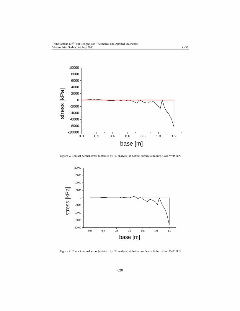
The figures 7 and 8 present compressive stress at the base of the wall. The stress concentrations at the right bottom corner indicate developing of a compressive diagonal strut and stress releasing at the left bottom zone. The high peaks of compression stresses indicate possible crushing of masonry.
0
20
40
60
80
100
120
140
0 1 2 3 4
Horizontal displacement (mm)
H (
kN
)
V=250kN
V=150kN
Figure 5. Horizontal force - displacement curves for two cases (vertical loads V=150kN and V=250kN)
Figure 6. Experimentally [18] and numerically obtained failure pattern (deformation scale 30:1)
625
Third Serbian (28th Yu) Congress on Theoretical and Applied Mechanics Vlasina lake, Serbia, 5-8 July 2011 C-32
0.0 0.2 0.4 0.6 0.8 1.0 1.2-10000
-8000
-6000
-4000
-2000
0
2000
4000
6000
8000
10000st
ress
[kP
a]
base [m]
Figure 7. Contact normal stress (obtained by FE analysis) at bottom surface at failure. Case V=150kN
0.0 0.2 0.4 0.6 0.8 1.0 1.2-20000
-15000
-10000
-5000
0
5000
10000
15000
20000
stre
ss [k
Pa]
base [m]
Figure 8. Contact normal stress (obtained by FE analysis) at bottom surface at failure. Case V=250kN
626

Third Serbian (28th Yu) Congress on Theoretical and Applied Mechanics Vlasina lake, Serbia, 5-8 July 2011 C-32
In table 2 there is an assessment of global moduli of a masonry wall based on response obtained by finite element model. Ew modulus is obtained from the numerical simulation of initial loading process with V=250kN. The global shear modulus is extracted from the response with horizontal load H=40kNH=0,35Hult assuming that the total horizontal displacement is the result of bending and shear deformation.
Global moduli of masonry wall
Finite element
Exp. ref. [18 ]
Ew (GPa) 4,8 4,1
Gw(GPA) 1,77 1,67
Table 2.Young’s and shear moduli of the masonry wall extracted from finite element analysis and experiment
5. Conclusions A micro-modelling of masonry walls subjected to static shear in-plane loading is presented. The model has been validated by comparing the results with available experiments. After a number of numerical tests we may say that in our research overall response of masonry wall can be well predicted from the point of view of failure loads. During the loading process, a compressive diagonal strut was formed from the top-left to the bottom right corner. The cracking and shearing-off was spread in a relatively larger zone and was not localized in a „step mode mechanism“. The further work, including developing user defined material models in Abaqus finite element code, is necessary in order to obtain robust and reliable various failure modes of masonry walls.
Acknowledgement. The study presented in this paper is the part of the research financed by the Ministry of science and technology, Republic of Serbia.
References [1] Tomaževič M, Gams M
and. Lu S. (2009), Modelling of shear failure mechanism of masonry walls, Proceedings of the 11th Canadian Masonry Symposium, Toronto, Canada. [2] Tomaževič M., Weiss P (1994). Seismic behaviour of plain and reinforced masonry buildings, Journal of Structural Engineering, ASCE, 120 (2), 323-338 [3] Benedetti D., Pezzoli P. and Carydis P, (1998), Shaking table tests on 24 simple masonry buildings, Earthquake Engin. Struct. Dyn. Vol. 27. [4] Muravljov M, Zakić D (2009), Izveštaj o ispitivanju parametara čvrstoće zidova od opeke u sklopu objekta Kliničkog centra – Instituta za patlogiju u Beogradu, Izveštaj 97/2009, Institut za materijale i konstrukcije, Gradjevinski fakultet u Beogradu. [5] Shear test on masonry panels, Literature survey and proposal for experiments (2004), TNO report 2004/CI/R0171, TNO Building and construction research
627

Third Serbian (28th Yu) Congress on Theoretical and Applied Mechanics Vlasina lake, Serbia, 5-8 July 2011 C-32
[6] Schermer D. (2004), Experimental and Numerical Investigations on the Behaviour Of Unreinforced Masonry Buildings Under Seismic Loadings, Proceedings of the 13th International Brick and Block Masonry Conference, Amsterdam. [7] Graubner C. A, T. Kranzle T (2005), Shear Design of Unreinforced Masonry Panels - Basic Assumptions And Comparison Of Different Standards . 10th Canadian Masonry Symposium, Banff, Alberta, Canada [8] Lourenco, P.B., Rots, J.G,(1997). Multisurface Interface Model for Analysis of Masonry Structures, Journal of Engineering Mechanics, ASCE, Vol.123, No. 7, 660-668. [9] Lourenço, P.B. J.G. Rots, J. Blaauwendraad, Continuum model for masonry: Parameter estimation and validation, Journal of Structural Engineering ASCE, 124(6), 1998, pp. 642-652. [10] Daryan A S et al (2009) A Study of the Effect of Infilled Brick Walls on Behavior of Eccentrically Braced Frames Using Explicit Finite Elements Method, American J. of Engineering and Applied Sciences 2 (1): 96-104,. [11] Lotfi, H. R. and Shing, P. B. (1991). An appraisal of smeared crack models for masonry shear wall analysis. Computers and Structures Vol.41(3): pp.413-425. [12] Madan A, Reinhorn a. M, Mander J. B., and Valles R.E (1996), Modeling of Masonry Infill Panels for Structural Analysis, Journal of Structural Engineering, ASCE, pp. 1295–1302. [13] Marcari G, Fabbrocino G, Manfredi G, Prota A, (2007) Experimental And Numerical Evaluation of Tuff Masonry Panels Shear Seismic Capacity, Proceedings of the 10th North American Masonry Conference, St. Louis, Missouri, USA. [14] Gambarotta, L. and Lagomarsino S. (1997) Damage models for the seismic response of brick masonry shear walls. Part II: The continuum model and its applications, Earthquake Eng. Struct. Dyn., 26: 441-462. [15] Smyrou E et al (2006) An implementation And Verification Of A Masonry Panel Model For Nonlinear Pseudo-Dynamic Analysis Of Infilled RC Frames, First European Conference On Earthquake Engineering And Seismology Geneva, Switzerland, Paper Number: 355 [16] Salatić R, Mandić R, Perović Z (2010) Modeliranje zidane ispune u seizmičkom proračunu, Savetovanje Zemljotresno inženjerstvo i inženjerska seizmologija, Divčibare 2010, pp. 107-112. [17] Magenes G, (2006), Masonry Building Design in Seismic Areas: Recent Experiences and Prospects from a European Standpoint, First European Conference on Earthquake Engineering and Seismology (a joint event of the Geneva, Switzerland, paper number: keynote address k9 [18] Charry Ablanque J. A. (2010) Experimental Study Of Masonry Wall Behaviour Under Lateral Stress, Tesis Doctoral Departamento de ingenieria de la construcción, Universidad Politécnica de Cataluña, Spain [19] Stupkiewicz S. Mróz Z, (2001) Modelling Of Friction And Dilatancy Effects at Brittle Interfaces For Monotonic And Cyclic Loading, Journal Of Theoretical and Applied Mechanics, 3, 39, pp. 707-739. [20] Van Der Pluijm, R. (1992). Material properties of masonry and its components under tensile and shear, Proc. 6th Canadian Masonry Symp., Canada, 675 – 686. [21] Eurocode 6, Design of masonry structures - Part 1-1: Common rules for reinforced and unreinforced masonry structures, CEN: Brussels. [22] Abaqus, ver. 6.9 (2008), Users manual, Dassault Systèmes Simulia Corp., Providence, RI, USA.
628

Third Serbian (28th Yu) Congress on Theoretical and Applied Mechanics Vlasina lake, Serbia, 5-8 July 2011 C-33
NUMERICAL AND EXPERIMENTAL DIAGNOSTIC OF DYNAMIC BEHAVIOR OF THE ROTOR-EXCAVATOR CONSTRUCTION
T. Maneski1, P. Jovančić2, D. Ignjatović2, V. Milošević-Mitić1, N. Trišović1
1 Faculty of Mechanical Engineering The University of Belgrade, Kraljice Marije 16, 11120 Belgrade 35 e-mail: [email protected] 2 Faculty of Mining and Geology The University of Belgrade, Đušina 7, 11120 Belgrade 35
Abstract. Dynamic behaviour of a rotor-excavator construction is of crucial importance for proper and reliable operation. Numerical and experimental procedure shown that these structures failed due to incorrect operational parameters related to the vibration of complete supporting structures. Therefore, the base for rehabilitation and reconstruction is a dynamic diagnostics of the structure. This analysis involves a computer calculation by the finite elements method with the mandatory experimental measurements. This enables determination of the actual behaviour of structure, reliable prediction of its response in operation, determination of the cause for poor behaviour or failure, assessment of service life time of reliable operation and the scope of revitalization. Operational problems developed mostly from improper geometry design. Presented methodology is inevitable during the engineering analysis of excavator structure. This approach is justified due to low costs with a very high level of results.
1. Introduction
Rotor-excavators are very complex sistems with a great number of functionaly important elements. Working life of the rotor excavator depends of the stable of the steel structure. For a drive system we have very clear criteriums about replacement or rehabilitation which is not case for the steel structure. So, experimental tests and visual analysis have to give validation of the numerical model based on the finite element method FEM. FEM and experimental messurements are the main tools in the proces of the construction accompaniment [1].
The basis for structural performance diagnostics is the computer modelling and structural analysis calculation software with the application of finite element numerical method throughout static, dynamic and thermal calculation of consisting structural elements.
Program KOMIPS [2] allows modelling and the calculation of complex structures and problems, determination of real displacements and stresses and real structural behaviour including the consisting elements, it gives a reliable forecast of structural behaviour in service and depicts the parameters for decision making (operating regime, repairs, reconstructions, revitalizations, optimizations, confirmations of selected solution variants), poor performance sample identification or structural deterioration, service life estimation and time of reliable operation efficiency. Every improvement of structural performance that can be reached by this approach allows service life extension and increase of reliability.
The developed system KOMIPS includes specific calculus for closer defining structural state and behaviour. The equivalent stress, according to the Huber–Hencky–Misses theory,
629
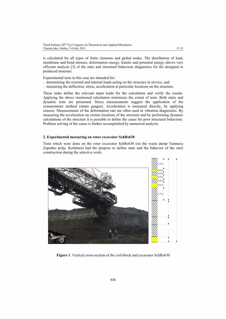
Third Serbian (28th Yu) Congress on Theoretical and Applied Mechanics Vlasina lake, Serbia, 5-8 July 2011 C-33
is calculated for all types of finite elements and global nodes. The distribution of load, membrane and bend stresses, deformation energy, kinetic and potential energy allows very efficient analysis [3] of the state and structural behaviour diagnostics for the designed or produced structure.
Experimental tests in this case are intended for: – determining the external and internal loads acting on the structure in service, and – measuring the deflection, stress, acceleration at particular locations on the structure.
These tasks define the relevant input loads for the calculation and verify the results. Applying the above mentioned calculation minimizes the extent of tests. Both static and dynamic tests are presumed. Stress measurements suggest the application of the extensometer method (strain gauges). Acceleration is measured directly, by applying sensors. Measurements of the deformation rate are often used in vibration diagnostics. By measuring the acceleration on certain locations of the structure and by performing dynamic calculations of the structure it is possible to define the cause for poor structural behaviour. Problem solving of the cause is further accomplished by numerical analysis.
2. Experimental messuring on rotor excavator SchRs630
Tests which were done on the rotor excavator SchRs630 (on the waste dump Tamnava Zapadno polje, Kolubara) had the purpose to define state and the bahavior of the steel construction during the selective work.
1.7 m
0.5 m
0.6 m
0.3 m
0.6 m
0.2 m
1.4 m
Figure 1. Vertical cross-section of the coil-block and excavator SchRs630
630

Third Serbian (28th Yu) Congress on Theoretical and Applied Mechanics Vlasina lake, Serbia, 5-8 July 2011 C-33
All parameters were obtained during work, for rigid highs of cuts: 0.5-0.7 m, 1-1.2 m, 2-2.2 m and for 5-7 m. The whole high of the coil-block was 10.5 m.
The characteristis place for the measuring was on the lug of the slice of the will-excavator.
Figure 2 presents appropriate measuring place.
Figure 2. Measuring place
Stress was measured using three strain gauges. On the same time, accelerations were obtaining. Instalation of the strain gauges was done on the static-loaded construction.
Measurings were done in next order:
1. Stress and acceleration for cut-high of h = 5.3 m and for advent of 40 cm and 20 cm (for left and right direction),
2. Stress and acceleration for cut-high of h = 2 m and for advent of 70 cm and 35 cm (for left and right direction),
3. Stress and acceleration for cut-high of h = 1 m and for advent of 60 cm and 30 cm (for left and right direction),
4. Stress and acceleration for cut-high of h = 0.7 m and for advent of 80 cm and 40 cm (for left and right direction).
Obtained diagrems for stress accession and for acceleration in time and frequent domain are presented on figure 3 for the first case of loading.
631

Third Serbian (28th Yu) Congress on Theoretical and Applied Mechanics Vlasina lake, Serbia, 5-8 July 2011 C-33
0.00 0.20 0.40 0.60 0.80 1.00 1.20 1.40 1.60 1.80 2.00Time [Sec.]
-1.0
-0.5
0.0
0.5
1.0
0.00 0.20 0.40 0.60 0.80 1.00 1.20 1.40 1.60 1.80 2.00
Time [Sec.]
-1.0
-0.5
0.0
0.5
2.00 4.00 6.00 8.00 10.00 12.00Frequency [Hz]
0.00
1.00-02
2.00-02
3.00-02
4.00
Left
1.00 2.00 3.00 4.00 5.00 6.00 7.00 8.00 9.00 10.00Frequency [Hz]
0.00
1.00-02
2.00-02
3.00-02
4.00-02
5.00-02
Right
Figure 3. Stress, accelerations in time and frequent domain in the first case
During left cuting, stress accession was between 50-55 N/mm2 at the begining of the process and then decreased to 15-25 N/mm2. Acceleration in time domain was to 1G, which was satisfied. But, low frequences to 10 Hz was obtained on the steel structure.
During right cuting, stress accession was as in the previous case 50-55 N/mm2 at the begining of the process and later 10-40 N/mm2. Acceleration in time domain was to 0.8G, which was satisfied. Diging frequecy of 2.7 Hz wasn’t dominant.
Figure 4 shows obtained diagrams for the second group of measurings.
632

Third Serbian (28th Yu) Congress on Theoretical and Applied Mechanics Vlasina lake, Serbia, 5-8 July 2011 C-33
0.00 0.20 0.40 0.60 0.80 1.00 1.20 1.40 1.60 1.80 2.00Time [Sec.]
-1.0
-0.5
0.0
0.5
1.0
0.00 0.20 0.40 0.60 0.80 1.00 1.20 1.40 1.60 1.80 2.00 2.20
Time [Sec.]
-1.0
-0.5
0.0
0.5
1.00 2.00 3.00 4.00 5.00 6.00 7.00 8.00 9.00 10.00 11.00Frequency [Hz]
0.00
1.00-02
2.00-02
3.00-02
4.00-02
Left, 70 cm
5.00 10.00 15.00 20.00 25.00 30.00 35.00 40.00 45.00 50.00Frequency [Hz]
0.00
5.00-02
0.1
0.1
0.2
Left, 35 cm
Figure 4. Accelerations in time and frequent domain in the seccond case
Left cuting of 70 cm gives stress accession of maximal 60-70 N/mm2 at the begining and about 20-40 N/mm2 later. Stress was high but in limited value. Acceleration was to 1G, which was satisfied. The amplitude of the characteristic frequences was to 0.04 m/s2.
Left cuting of 35 cm gives stress accession of maximal 45-50 N/mm2 at the begining and about 15-30 N/mm2 later. Acceleration was to 1G, which was satisfied. The amplitude of the characteristic frequences was to 0.15 m/s2.
Figure 5 shows obtained diagrams for the third group of measurings.
0.00 0.20 0.40 0.60 0.80 1.00 1.20 1.40 1.60 1.80 2.00Time [Sec.]
-0.5
0.0
0.5
cce e at o [ /s ]
0.00 0.20 0.40 0.60 0.80 1.00 1.20 1.40 1.60 1.80 2.00
Time [Sec.]
-1.0
0.0
1.0
cce e at o [ /s ]
633

Third Serbian (28th Yu) Congress on Theoretical and Applied Mechanics Vlasina lake, Serbia, 5-8 July 2011 C-33
1.00 2.00 3.00 4.00 5.00 6.00 7.00 8.00 9.00 10.00 11.00Frequency [Hz]
0.00
2.00-02
4.00-02
6.00-02
8.00-02
0.1
0.1
[ / ]
Right, 60 cm
1.00 2.00 3.00 4.00 5.00 6.00 7.00 8.00 9.00 10.00 11.00Frequency [Hz]
0.00
5.00-02
0.1
0.1
0.2
0.3
Right, 30 cm
Figure 5. Accelerations in time and frequent domain in the third case of loading
Right cutting of 60 cm gives next values: - Sterss accession of 30-40 N/mm2 the the begining and 10-25 N/mm2 later, - Acceleration in time domain 0.75G maximum, - Low frequencies to 10 Hz of steel construction, - Amplitude of the characteristic frequences to 0.13 m/s2.
Right cutting of 30 cm gives next values: - Sterss accession of 25-30 N/mm2 the the begining and 10-20 N/mm2 later, - Acceleration in time domain 1.2G maximum, - Amplitude of the characteristic frequences to 0.25 m/s2.
0.00 0.20 0.40 0.60 0.80 1.00 1.20 1.40 1.60 1.80 2.00 2.20Time [Sec.]
-0.5
0.0
0.5
cce e at o [ /s ]
0.00 0.20 0.40 0.60 0.80 1.00 1.20 1.40 1.60 1.80 2.00 2.20
Time [Sec.]
-0.5
0.0
0.5
cce e at o [ /s ]
Left, 80 cm Right, 40 cm
Figure 6. Stress and accelerations in time domain in the fourth case
634

Third Serbian (28th Yu) Congress on Theoretical and Applied Mechanics Vlasina lake, Serbia, 5-8 July 2011 C-33
Obtained results are presented in next table.
Table 1. Results in the fourth case of loading Sterss
accession Acceleration Amplitude Frequencies of steel
structure Left, 80 cm 35-45 N/mm2
10-25 N/mm2 0.7G 0.03 m/s2 to 10 Hz
Right, 40 cm 35-45 N/mm2
10-25 N/mm2 0.7G 0.085 m/s2 to 10 Hz
3. Numerical model of the rotor-excavator steel structure
Dynamic behaviour diagnostics of the operating wheel cantilever beam was done using program package KOMIPS. Shown below are major oscillation forms of the operating wheel for two outermost cantilever positions (A and B).
Position A: f01 = 0.8 Hz, f02 = 1.3 Hz Position A: f03 = 2.3 Hz, f04 = 3.3 Hz
Position B: f01 = 0.8 Hz, f02 = 1.6 Hz Position B: f03 = 2.7 Hz, f04 = 3.4 Hz
Figure 7. Main oscillating forms of operating wheel cantilever in positions A and B
The main diagnostic element is defined by the unloading range (number of buckets operating wheel revolutions). The unloading number must correlate to eigen-value oscil-lations of the operating wheel cantilever beam. From the cantilever dynamics point of view,
635

Third Serbian (28th Yu) Congress on Theoretical and Applied Mechanics Vlasina lake, Serbia, 5-8 July 2011 C-33
the number of unloads should be within (1.6÷2.3 Hz) 60 sec = 96÷138, i.e. for a 23 bucket wheel, the revolutions should be 4.17 to 6 min–1.
4. The conclusion
Diagnostic of the behaviour of the steel structure of the rotor excavator SchRs630 was based on the numerical model and the experimental tests. Obtained results show:
- load-measurings were done in dynamic-load state of the rotor excavator, - higher stress accessions were propper to higher cut-highes and steps, - measuring results were satisfied and in limitid values, - experimental results validated numerical model.
Acknowledgement. This work is a contribution to the Ministry of Science and Technological Development of Serbia funded project TR 35040 and TR 35011.
REFERENCES [1] T. Maneski, V. Milošević-Mitić, Numerical and experimental diagnostic of
structural strength, Structural integrity and life, 10 (1) (2010) 3-10. [2] G.M. Zloković, T. Maneski, M. Nestorović, Group theoretical formulation of
quadrilateral and hexahedral isoparametric finite elements, COMPUTERS & STRUCTURES, 82 (11-12) (2004) 883-899.
[3] N. Trišović, T. Maneski, D. Kozak, Developed procedure for dynamic reanalysis of structures, Strojarstvo - Journal for Theory and Application in Mechanical Engineering, 52 (2) (2010) 147-158.
[4] P. Jovančić, D. Ignjatović, T. Maneski, P., Diagnosis of behaviour for support steel structure at a bucket wheel excavators, Handbook Machine design (editor S. Kuzmanović), Faculty of technical sciences University of Novi Sad (2008) pp.383-388.
[5] P. Jovančić, D. Ignjatović, T. Maneski, Analysis of loading steel structure of bucket wheel excavator by stress condition measuring, Proc. 26th Danubia-Adria Symposium on Advances in Experimental Mechanics, September 23 – 26. 2009, Leoben, Austria (2009) p.87-88.
636

Third Serbian (28th Yu) Congress on Theoretical and Applied Mechanics Vlasina lake, Serbia, 5-8 July 2011 C-34
SOME APPLICATIONS AND CONSTRAINTS OF THE FEM WITHIN THE MODAL ANALYSIS OF THE STRUCTURES
Lj. Markovic 1, D. Ruzic 2, H. Hertha-Haverkamp 3, C. Kardelky 4
1 Tensor GmbH Nordbahnhofstraße 16, D-70191 Stuttgart, Germany e-mail: [email protected] 2 Faculty of Mechanical Engineering, The University of Belgrade, Kraljice Marije 16, 11120 Belgrade 35, Serbia e-mail: [email protected] 3 Hochschule Reutlingen Alteburgstraße 150, D-72762 Reutlingen, Germany e-mail: [email protected] 4 Hochschule Pforzheim Tiefenbronner Straße 65, D-75175 Pforzheim, Germany e-mail: [email protected]
Abstract. The contributions to the dynamic analysis of machine parts or of a group of machines as well as the algorithmic concept are given. Particular attention is paid to the modal analysis. The FEM is a very efficient method for obtaining a very quick Feed-Back – the response of the system if the input parameters of the system are given in advance. But as very often the protection of the data (e.g. the engine parameters in motor vehicle industry) is at a very high level one will meet just the inverse problem – to determine the load vector starting from the known dynamic response. It is well known that the resonant frequency field represents the particular importance for the calculations. As the experimental measurements are usually very expensive and as the rule, in the case of the dynamic analysis, they are performed only once, the relevant mathematical or FEM models are of very high importance. On the basis of theoretical knowledge of the problems from one side and of the practical experience from the other, the authors propose an algorithm for the application of the vibration analysis, where the calculation of one exhaust pipe is given as an example. The interaction between experimental measurements and the calculation is shown. The MAC-analysis, one of usually applied methods in the structural dynamics for the comparison of calculated and measured eigen-vectors, is used for the explanation of that interaction. The influence of the MAC-Matrix on the sensitive analysis as well as on the calculation of the substructure is explained.
1. Introduction` The modal analysis although by its nature expensive one is one of the most important methods in the numerical analysis of mechanical systems. Together with the development of new hardware having more outstanding performances, from one side, and with trends of avoiding expensive experiments, from the other, the modal analysis becomes more and more important in the numerical analysis. Although the vibration analysis is performed in the finite time domain, a great part of responsibility is transferred from the measurements to the calculations. That is quite understandable because it is too expensive to perform a new experiment if only some geometrical parameters (e.g. profile thickness) or the material are changed. The simultaneous intentions of avoiding expensive experiments and of obtaining quick results often yield to some contradictions between the time and the available
637

Third Serbian (28th Yu) Congress on Theoretical and Applied Mechanics Vlasina lake, Serbia, 5-8 July 2011 C-34
resources. The efficiency of one FEM program depends on its structure and on the quantity of available processors that are needed for its performing. The intention of the paper that follows is to prove that when the modal analysis is in question the universal FEM program satisfying all requirements does not exist, and to point to some methods for solving the problems that are met in practice. Some specific industrial requirements that one FEM program can not always and completely satisfy are often faced and that is why some additional tools for solving real problems are needed. 2. Basic equations In the domain of modal analysis the starting point is the system of differential equations
)t(Fq Kq Dq M , (1)
Where: M – Mass matix, D – Damping matrix, K – Stiffness matrix,
)t(F – Load vector,
)t(qq - Displacement vector – the dynamic response of the system to given loads.
For one discrete mechanical system, q represents the displacement field in nodal points. It is not necessary to know the displacement field in all nodal points as the output but it is enough to know only the system response in the points in which the measurements were performed. These points, i.e. their coordinates, are taken from the measurements and corresponding nodal points are found in the FEM model. These points are suitably chosen in the mechanical system in order to obtain significant information about the spectral and modal behavior of the system.
Fig. 1.Generalized mechanical model for the analysis
If there are n points (Fig. 1) then the response at the kth point MPk will be denoted by qk and corresponding components by uk,vk,wk or
638

Third Serbian (28th Yu) Congress on Theoretical and Applied Mechanics Vlasina lake, Serbia, 5-8 July 2011 C-34
k
k
k
kM
w
v
u
q , (2)
The total displacement vector is given by
nM
3M
2M
1M
M
q
.
.
q
q
q
q , (3)
or, through the corresponding components, by
nnn222111T
M w.v.u.....I.w.v.u.I.w.v.uq (4)
From the mathematical point of view, there exists such an equivalent system that gives the identical displacement, or there exists a system of differential equations
)t(FqKqDqM eqeqeqeq (5)
Where:
eqM – Mass matrix,
eqD – Damping matrix,
eqK – Stiffness matrix,
)t(Feq – Load vector,
for the equivalent system that has to be determined. The importance of the formulation of the equivalent model will be noticed later. 3. Modal analysis The authors present the algorithm in the schematic form in order to show what a modal analysis applied to the calculation of one mechanical system is supposed to look like. The standard input consists of the geometry of the model, where material data and boundary conditions are defined in advance and where also the springs with their axial and torsional stiffnsses (Fig.1) are introduced.
639
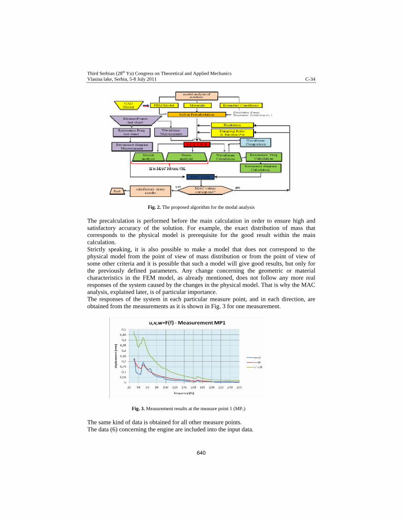
Third Serbian (28th Yu) Congress on Theoretical and Applied Mechanics Vlasina lake, Serbia, 5-8 July 2011 C-34
Fig. 2. The proposed algorithm for the modal analysis
The precalculation is performed before the main calculation in order to ensure high and satisfactory accuracy of the solution. For example, the exact distribution of mass that corresponds to the physical model is prerequisite for the good result within the main calculation. Strictly speaking, it is also possible to make a model that does not correspond to the physical model from the point of view of mass distribution or from the point of view of some other criteria and it is possible that such a model will give good results, but only for the previously defined parameters. Any change concerning the geometric or material characteristics in the FEM model, as already mentioned, does not follow any more real responses of the system caused by the changes in the physical model. That is why the MAC analysis, explained later, is of particular importance. The responses of the system in each particular measure point, and in each direction, are obtained from the measurements as it is shown in Fig. 3 for one measurement.
Fig. 3. Measurement results at the measure point 1 (MP1)
The same kind of data is obtained for all other measure points. The data (6) concerning the engine are included into the input data.
640
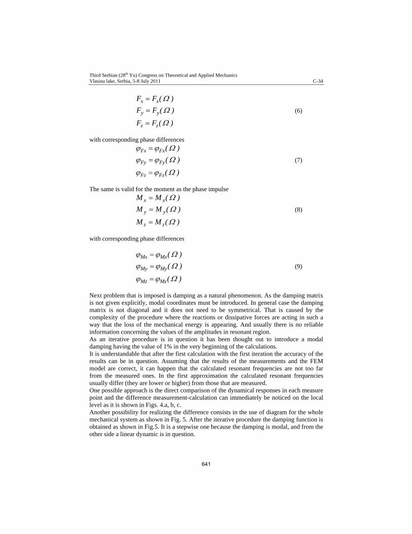
Third Serbian (28th Yu) Congress on Theoretical and Applied Mechanics Vlasina lake, Serbia, 5-8 July 2011 C-34
)(FF
)(FF
)(FF
zz
yy
xx
(6)
with corresponding phase differences
)(
)(
)(
FzFz
FyFy
FxFx
(7)
The same is valid for the moment as the phase impulse
)(MM
)(MM
)(MM
zz
yy
xx
(8)
with corresponding phase differences
)(
)(
)(
MzMz
MyMy
MxMx
(9)
Next problem that is imposed is damping as a natural phenomenon. As the damping matrix is not given explicitly, modal coordinates must be introduced. In general case the damping matrix is not diagonal and it does not need to be symmetrical. That is caused by the complexity of the procedure where the reactions or dissipative forces are acting in such a way that the loss of the mechanical energy is appearing. And usually there is no reliable information concerning the values of the amplitudes in resonant region. As an iterative procedure is in question it has been thought out to introduce a modal damping having the value of 1% in the very beginning of the calculations. It is understandable that after the first calculation with the first iteration the accuracy of the results can be in question. Assuming that the results of the measurements and the FEM model are correct, it can happen that the calculated resonant frequencies are not too far from the measured ones. In the first approximation the calculated resonant frequencies usually differ (they are lower or higher) from those that are measured. One possible approach is the direct comparison of the dynamical responses in each measure point and the difference measurement-calculation can immediately be noticed on the local level as it is shown in Figs. 4.a, b, c. Another possibility for realizing the difference consists in the use of diagram for the whole mechanical system as shown in Fig. 5. After the iterative procedure the damping function is obtained as shown in Fig.5. It is a stepwise one because the damping is modal, and from the other side a linear dynamic is in question.
641

Third Serbian (28th Yu) Congress on Theoretical and Applied Mechanics Vlasina lake, Serbia, 5-8 July 2011 C-34
Fig. 4,a. Comparative analysis of dynamical response in x-direction
Fig. 4,b. Comparative analysis of dynamical response in y-direction
4. MAC-Matrix (Modal Assurance Criterion) Anyhow, one of very efficient methods today for the determination of the differences from the measured values is so called MAC-Matrix (Modal Assurance Criterion). A MAC-matrix element is defined as a normalized scalar product of the measured and calculated eigen-vectors.
)vv)(vv(
)vv()j,i(MAC )j(
measT)j(
meas)i(
calcT)i(
calc
2)j(meas
T)i(calc
(10)
642
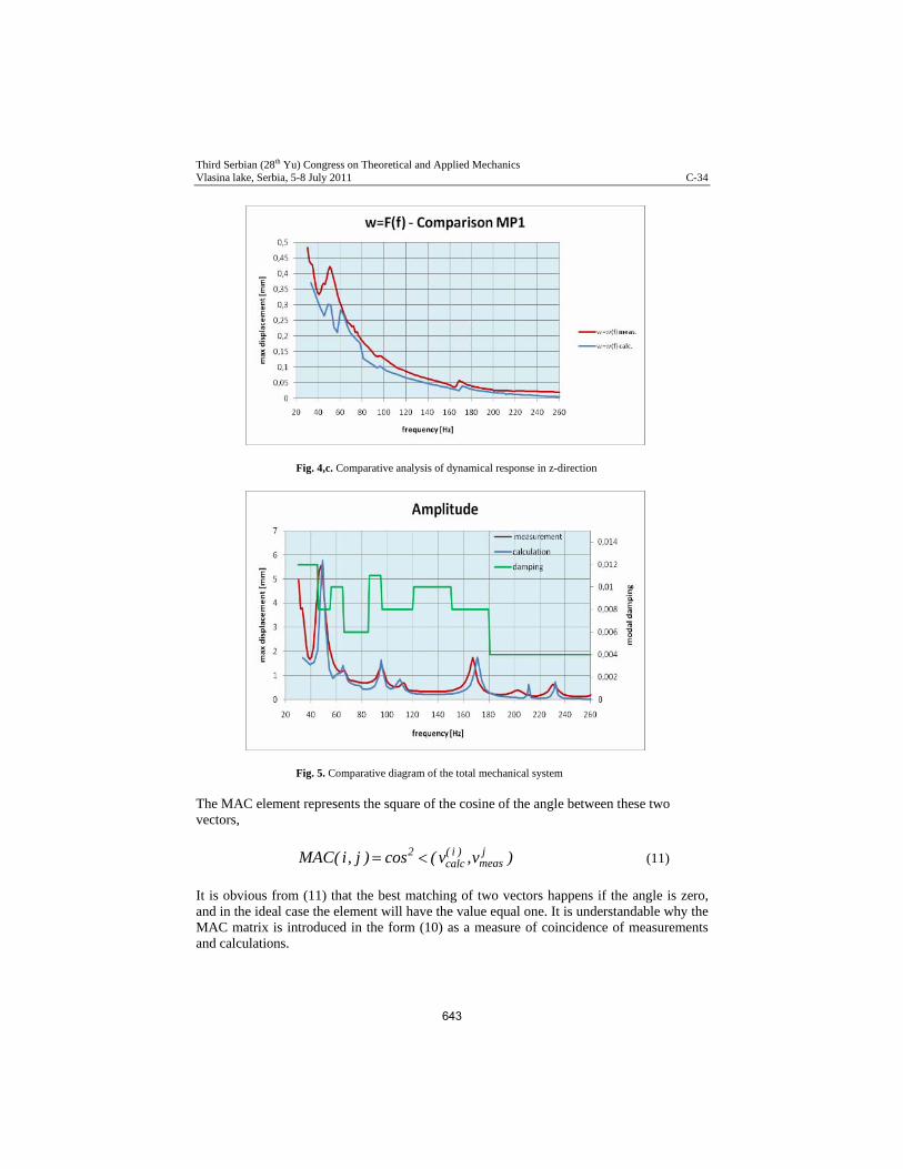
Third Serbian (28th Yu) Congress on Theoretical and Applied Mechanics Vlasina lake, Serbia, 5-8 July 2011 C-34
Fig. 4,c. Comparative analysis of dynamical response in z-direction
Fig. 5. Comparative diagram of the total mechanical system
The MAC element represents the square of the cosine of the angle between these two vectors,
)v,v(cos)j,i(MAC jmeas
)i(calc
2 (11)
It is obvious from (11) that the best matching of two vectors happens if the angle is zero, and in the ideal case the element will have the value equal one. It is understandable why the MAC matrix is introduced in the form (10) as a measure of coincidence of measurements and calculations.
643
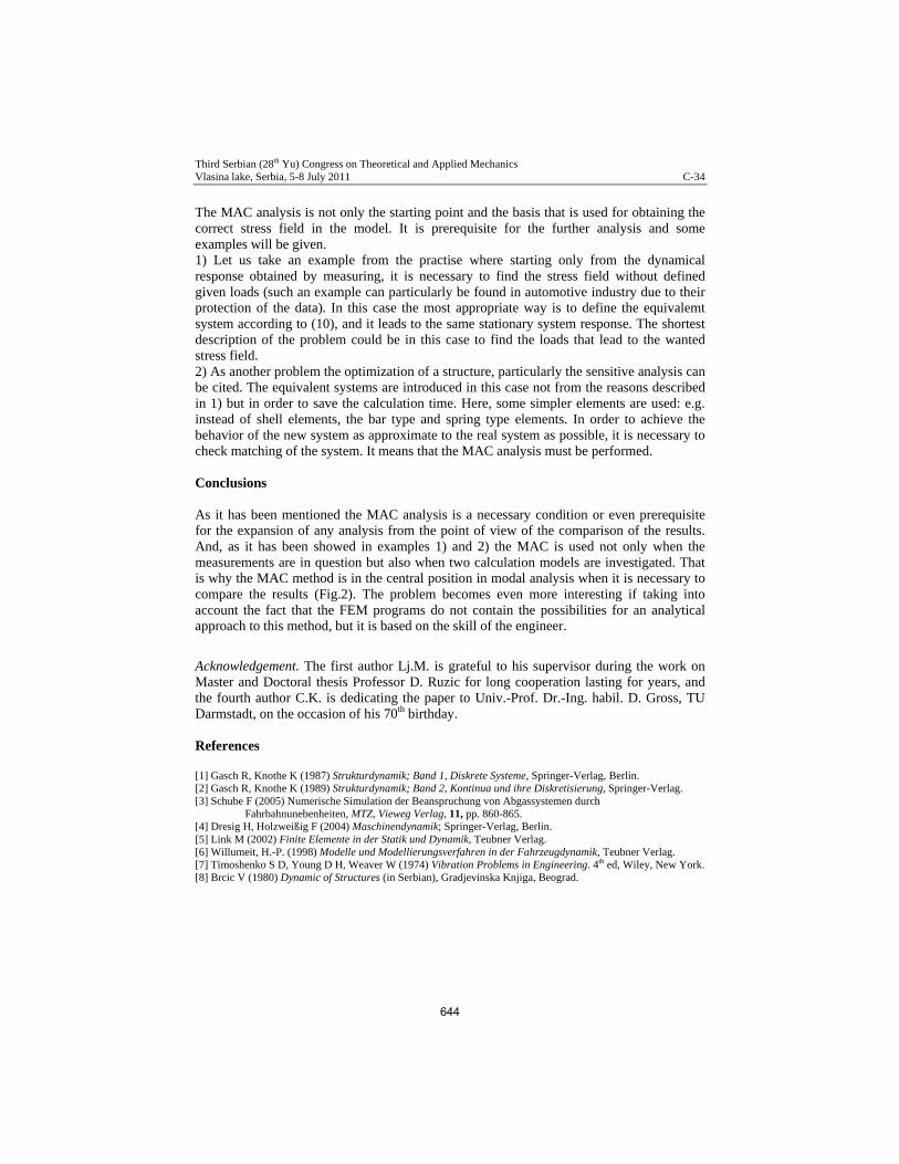
Third Serbian (28th Yu) Congress on Theoretical and Applied Mechanics Vlasina lake, Serbia, 5-8 July 2011 C-34
The MAC analysis is not only the starting point and the basis that is used for obtaining the correct stress field in the model. It is prerequisite for the further analysis and some examples will be given. 1) Let us take an example from the practise where starting only from the dynamical response obtained by measuring, it is necessary to find the stress field without defined given loads (such an example can particularly be found in automotive industry due to their protection of the data). In this case the most appropriate way is to define the equivalemt system according to (10), and it leads to the same stationary system response. The shortest description of the problem could be in this case to find the loads that lead to the wanted stress field. 2) As another problem the optimization of a structure, particularly the sensitive analysis can be cited. The equivalent systems are introduced in this case not from the reasons described in 1) but in order to save the calculation time. Here, some simpler elements are used: e.g. instead of shell elements, the bar type and spring type elements. In order to achieve the behavior of the new system as approximate to the real system as possible, it is necessary to check matching of the system. It means that the MAC analysis must be performed. Conclusions As it has been mentioned the MAC analysis is a necessary condition or even prerequisite for the expansion of any analysis from the point of view of the comparison of the results. And, as it has been showed in examples 1) and 2) the MAC is used not only when the measurements are in question but also when two calculation models are investigated. That is why the MAC method is in the central position in modal analysis when it is necessary to compare the results (Fig.2). The problem becomes even more interesting if taking into account the fact that the FEM programs do not contain the possibilities for an analytical approach to this method, but it is based on the skill of the engineer.
Acknowledgement. The first author Lj.M. is grateful to his supervisor during the work on Master and Doctoral thesis Professor D. Ruzic for long cooperation lasting for years, and the fourth author C.K. is dedicating the paper to Univ.-Prof. Dr.-Ing. habil. D. Gross, TU Darmstadt, on the occasion of his 70th birthday. References [1] Gasch R, Knothe K (1987) Strukturdynamik; Band 1, Diskrete Systeme, Springer-Verlag, Berlin. [2] Gasch R, Knothe K (1989) Strukturdynamik; Band 2, Kontinua und ihre Diskretisierung, Springer-Verlag. [3] Schube F (2005) Numerische Simulation der Beanspruchung von Abgassystemen durch
Fahrbahnunebenheiten, MTZ, Vieweg Verlag, 11, pp. 860-865. [4] Dresig H, Holzweißig F (2004) Maschinendynamik; Springer-Verlag, Berlin. [5] Link M (2002) Finite Elemente in der Statik und Dynamik, Teubner Verlag. [6] Willumeit, H.-P. (1998) Modelle und Modellierungsverfahren in der Fahrzeugdynamik, Teubner Verlag. [7] Timoshenko S D, Young D H, Weaver W (1974) Vibration Problems in Engineering. 4th ed, Wiley, New York. [8] Brcic V (1980) Dynamic of Structures (in Serbian), Gradjevinska Knjiga, Beograd.
644

Third Serbian (28th Yu) Congress on Theoretical and Applied Mechanics Vlasina lake, Serbia, 5-8 July 2011 C-35
MICROMECHANICAL APPROACH TO INTEGRITY ASSESSMENT OF SURFACE DAMAGED PIPES
B. Medjo1,a, M. Rakin1, M. Arsić2, Ž. Šarkoćević3, A. Sedmak4 1 Faculty of Technology and Metallurgy, University of Belgrade, Karnegijeva 4, 11120 Belgrade, Serbia 2 Institute for Testing of Materials - IMS, Bulevar vojvode Mišića 43, 11000 Belgrade, Serbia 3 High Technical School of Professional Studies Nušićeva 6, 38227 Zvečan, Serbia 4 Faculty of Mechanical Engineering, University of Belgrade, Kraljice Marije 16, 11120 Belgrade, Serbia a e-mail: [email protected]
Abstract. During the service life, casing steel pipes for oil and gas drilling rigs are subjected to a corrosive atmosphere, along with high pressures and elevated temperatures. Hence, they are very susceptible to corrosion damages, often preceded by errors in design, manufacturing or mounting. The influence of corrosion defects to pipeline integrity is investigated by pressure test of a pipe with circular notches, machined in order to simulate actual defects. Micromechanical approach is applied to predict the damage development, and failure criterion is considered fulfilled when damage parameter reaches its critical value in the bottom of a notch. Several analytical expressions and numerical criterion based on von Mises stress value are used for estimation of the critical pressure in damaged pipeline, and solutions are compared with the predictions of micromechanical complete Gurson model.
1. Introduction Pipelines are the most economical and safest way for oil and gas exploitation and transport. Decrease in strength caused by the corrosion defects is very often encountered in these structures; it can endanger the work safety and even lead to catastrophic failures. Casing steel pipes used in the oil drilling rigs are subjected to a corrosive atmosphere, with coupled effects of high pressures and elevated temperatures during the service life. Hence, they are very susceptible to material degradation, often preceded by errors in design, construction, manufacturing, mounting and exploitation. The reliability of the oil and gas drilling rig systems is very important for continuous exploitation, as well as for environment protection. Many procedures for estimation of remaining strength of the pipes with corroded (local thin) areas have been developed, [1-8]. One of the solutions for assessment of corrosion defect influence to the pipe integrity is ASME B31G code [1]. Several other procedures are also derived from it, such as [2] (in the remainder of the text - modified ASME B31G) or RSTRENG [3]. Det Norske Veritas (DNV) published recommended practices [4] for determining corroded pipelines remaining strength under internal pressure and axial loading. FITNET procedures [5] also contain a module for estimating the remaining strength of pipelines with local corrosion damages.
645

Third Serbian (28th Yu) Congress on Theoretical and Applied Mechanics Vlasina lake, Serbia, 5-8 July 2011 C-35
Choi et al. [6] derived limit load solutions based on results of experimental and numerical analyses. Adib-Ramezani et al. [7] proposed integrity assessment of the pipes with defects under internal pressure based on a modification of SINTAP (Structural integrity assessment procedure) [9]. In this paper, a local criterion for maximum pressure in damaged casing pipe for drilling rigs, manufactured from API J55 steel, is discussed. Pressure test is conducted on a pipe segment capped at both ends. Corrosion defects were simulated by machining the circular notches, and the pipe was subjected to hydrostatic pressure to determine the spreading of plasticity in damaged areas. Local approach to fracture is applied to assess the failure criterion for damaged pipe, and the results are compared with existing solutions from the literature and a finite element stress-based criterion.
2. Experimental
2.1 Material API J55 steel is used for fabricating the examined seam casing pipe; yield strength 380 MPa, tensile strength 562 Mpa (more data about the material is given in [10]). Tensile properties are determined on round tensile (RT) specimens taken from the examined casing pipe. Figure 1 shows the strain state on the surface of the specimen obtained by stereometric measurement system Gom/Aramis [11] with two cameras and the software for data processing. This system enables determination of strain field on the surface of a structure, and a comparison with finite element solution is also given in Figure 1 (neck formation is marked by circles). Figure 2 shows the dependence of force on elongation; elongation is obtained by stereometric measurement.
Figure 1. Strain fields for RT specimen obtained by stereometric measurement system and finite element method
Having in mind that damage is modelled in this work using a micromechanical model, microstructural observation is conducted on samples cut from the pipe. This examination indicated presence of oxides, silicates and complex oxide inclusions. Two micro-
646
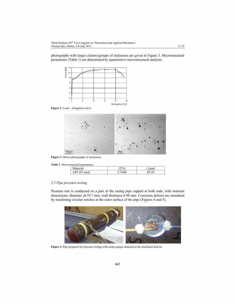
Third Serbian (28th Yu) Congress on Theoretical and Applied Mechanics Vlasina lake, Serbia, 5-8 July 2011 C-35
photographs with larger clusters/groups of inclusions are given in Figure 3. Microstructural parameters (Table 1) are determined by quantitative microstructural analysis.
Figure 2. Load – elongation curve
Figure 3. Micro-photographs of inclusions.
Table 1. Microstructural parameters.
Material f [%] λ [μm] API J55 steel 2.7648 69.39
2.2 Pipe pressure testing Pressure test is conducted on a part of the casing pipe capped at both ends, with nominal dimensions: diameter 139.7 mm, wall thickness 6.98 mm. Corrosion defects are simulated by machining circular notches at the outer surface of the pipe (Figures 4 and 5).
Figure 4. Pipe prepared for pressure testing with strain gauges attached at the machined defects.
647
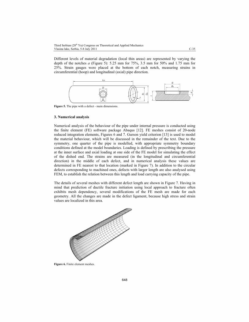
Third Serbian (28th Yu) Congress on Theoretical and Applied Mechanics Vlasina lake, Serbia, 5-8 July 2011 C-35
Different levels of material degradation (local thin areas) are represented by varying the depth of the notches a (Figure 5): 5.25 mm for 75%, 3.5 mm for 50% and 1.75 mm for 25%. Strain gauges were placed at the bottom of each notch, measuring strains in circumferential (hoop) and longitudinal (axial) pipe direction.
Figure 5. The pipe with a defect - main dimensions.
3. Numerical analysis Numerical analysis of the behaviour of the pipe under internal pressure is conducted using the finite element (FE) software package Abaqus [12]. FE meshes consist of 20-node reduced integration elements, Figures 6 and 7. Gurson yield criterion [13] is used to model the material behaviour, which will be discussed in the remainder of the text. Due to the symmetry, one quarter of the pipe is modelled, with appropriate symmetry boundary conditions defined at the model boundaries. Loading is defined by prescribing the pressure at the inner surface and axial loading at one side of the FE model for simulating the effect of the dished end. The strains are measured (in the longitudinal and circumferential direction) in the middle of each defect, and in numerical analysis these values are determined in FE nearest to that location (marked in Figure 7). In addition to the circular defects corresponding to machined ones, defects with larger length are also analysed using FEM, to establish the relation between this length and load carrying capacity of the pipe. The details of several meshes with different defect length are shown in Figure 7. Having in mind that prediction of ductile fracture initiation using local approach to fracture often exhibits mesh dependency, several modifications of the FE mesh are made for each geometry. All the changes are made in the defect ligament, because high stress and strain values are localized in this area.
Figure 6. Finite element meshes.
648

Third Serbian (28th Yu) Congress on Theoretical and Applied Mechanics Vlasina lake, Serbia, 5-8 July 2011 C-35
Figure 7. Finite element meshes of the defects
The results of the numerical analysis predict significantly larger strains in circumferential direction in comparison with longitudinal direction (up to 10 times), which is also measured during the experiment; results for depths 75 and 50% of the pipe wall thickness are shown in Figure 8.
0 5 10 15 20 25 30 35 40 450
1
2
3
4a/t = 0.75
Axial
Hoop
Str
ain
[%]
Experiment FEM
Pressure [MPa] 0 5 10 15 20 25 30 35 40 45
0.0
0.5
1.0
1.5
2.0a/t = 0.5
Axial
Hoop
S
tra
in [%
]
Experiment FEM
Pressure [MPa] (a) (b)
Figure 8. Comparison of strain values obtained experimentally and numerically, for defects with depth 75% (a) and 50% (b) of the pipe wall thickness.
4. Micromechanical modelling A significant accumulation of stress and plastic strain emerges in the bottom of a defect, which leads to development of ductile damage in this area. Gurson yield criterion (with damage parameter porosity or void volume fraction) is used for damage quantification in this work. The expression for plastic potential [13 - 15] is:
2* *21 12
3 32 cosh 1 0
2 2
ij ij mS S qq f q f
(1)
where σ denotes the flow stress of the material matrix, m is the mean stress and Sij is the stress deviator. Constitutive parameters q1 and q2 were introduced by Tvergaard [14] to improve the predictions of the Gurson model and f * is the damage function [15]:
649
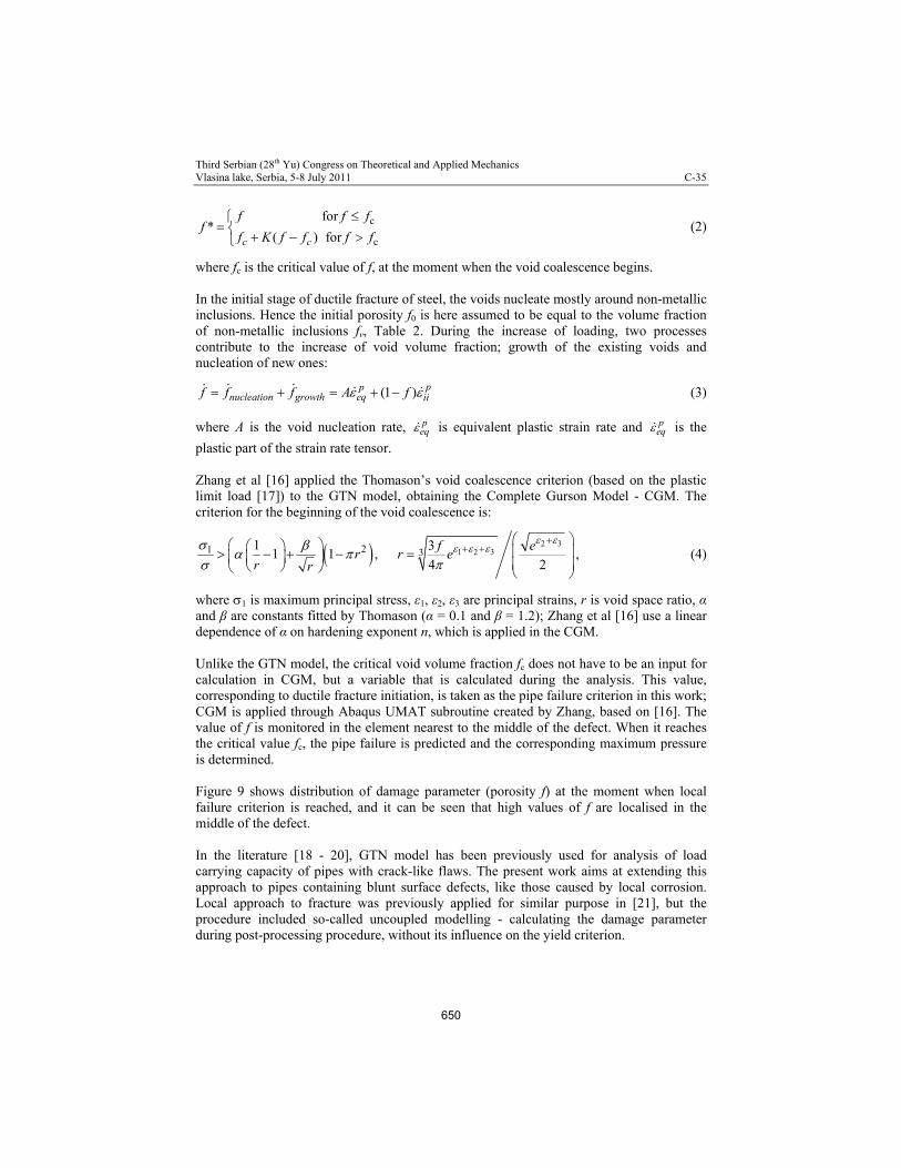
Third Serbian (28th Yu) Congress on Theoretical and Applied Mechanics Vlasina lake, Serbia, 5-8 July 2011 C-35
c
c
for *
( ) for c c
f f ff
f K f f f f
(2)
where fc is the critical value of f, at the moment when the void coalescence begins. In the initial stage of ductile fracture of steel, the voids nucleate mostly around non-metallic inclusions. Hence the initial porosity f0 is here assumed to be equal to the volume fraction of non-metallic inclusions fv, Table 2. During the increase of loading, two processes contribute to the increase of void volume fraction; growth of the existing voids and nucleation of new ones:
(1 ) ppnucleation growth eq iif f f A f (3)
where A is the void nucleation rate, peq is equivalent plastic strain rate and p
eq is the
plastic part of the strain rate tensor. Zhang et al [16] applied the Thomason’s void coalescence criterion (based on the plastic limit load [17]) to the GTN model, obtaining the Complete Gurson Model - CGM. The criterion for the beginning of the void coalescence is:
2 31 2 321 3
1 31 1 ,
4 2
f er r e
r r
, (4)
where 1 is maximum principal stress, ε1, ε2, ε3 are principal strains, r is void space ratio, α and β are constants fitted by Thomason (α = 0.1 and β = 1.2); Zhang et al [16] use a linear dependence of α on hardening exponent n, which is applied in the CGM. Unlike the GTN model, the critical void volume fraction fc does not have to be an input for calculation in CGM, but a variable that is calculated during the analysis. This value, corresponding to ductile fracture initiation, is taken as the pipe failure criterion in this work; CGM is applied through Abaqus UMAT subroutine created by Zhang, based on [16]. The value of f is monitored in the element nearest to the middle of the defect. When it reaches the critical value fc, the pipe failure is predicted and the corresponding maximum pressure is determined. Figure 9 shows distribution of damage parameter (porosity f) at the moment when local failure criterion is reached, and it can be seen that high values of f are localised in the middle of the defect. In the literature [18 - 20], GTN model has been previously used for analysis of load carrying capacity of pipes with crack-like flaws. The present work aims at extending this approach to pipes containing blunt surface defects, like those caused by local corrosion. Local approach to fracture was previously applied for similar purpose in [21], but the procedure included so-called uncoupled modelling - calculating the damage parameter during post-processing procedure, without its influence on the yield criterion.
650

Third Serbian (28th Yu) Congress on Theoretical and Applied Mechanics Vlasina lake, Serbia, 5-8 July 2011 C-35
Figure 9. Distribution of damage parameter - local failure criterion is reached.
5. Failure criteria comparison In addition to the micromechanical criterion, several solutions from literature are applied for calculation of the maximum pressure of the analysed pipe: ASME B31G code [1], modified ASME B31G [2, 3] and the solution of Choi et al. [6] (in the remainder of the paper - Choi’s solution/equation). Corresponding expressions are given in Table 2. Table 2. Expressions used for calculation of maximum pressure
ASME B31G
20 eL D t
212 31.1
2 11
3
max Ye
at tp
aDt M
2
1 0.8 e
LM
D t
20 eL D t 2
1.1 1
max Ye
t ap T
D t M
Modified ASME B31G
50 eL D t
22 2
1 0.6275 0.003375
e e
L LM
D t D t
50 eL D t
61 0.852
1.1 69 101
1 0.85
max Ye
at tp
aDt M
2
3.3 0.032 e
LM
D t
Choi’s solution
6L Rt
2
2 1 02
0.9
max mi
t L Lp C C C
D Rt Rt
2
2 0.1163 0.1053 0.0292
a aC
t t
2
1 0.6913 0.4548 0.1447
a aC
t t
2
0 0.06 0.1035 1.0
a aC
t t
6L Rt 1 02
max mi
t Lp C C
D Rt
1 0.0071 0.0126
aC
t
0 0.9847 1.1101
aC
t
651

Third Serbian (28th Yu) Congress on Theoretical and Applied Mechanics Vlasina lake, Serbia, 5-8 July 2011 C-35
In Table 2, a and L are defect depth and length, M is geometry correction factor, while Cj (j = 0..2) are coefficients in Choi’s equation. Geometry of the pipe is defined in Figure 5; De and Di represent the external and internal diameter of the pipe ( 2i eD D t ), while mean
pipe radius is ( ) / 4e iR D D .
Figure 10 shows the dependence of maximum pressure in a damaged pipeline on defect length for damage level 75%, obtained using expressions from Table 2, FE stress-based solution and CGM solution. FE stress-based failure criterion is considered to be fulfilled when von Mises stress value reaches the reference stress through the entire ligament; reference stress is chosen at 85 % of the ultimate tensile strength, as moderately conservative solution [22]. Two points for CGM at a damage length represent the limit values obtained using different element size (Figure 7) and formulation, as well as different load increments.
0 1 2 3 4 5 6
15
20
25
30
35
40
45
50
55
a/t = 0.75
L Rt
ASME B31G Modif. ASME B31G Choi et al. FEM (stress-based crit.) CGM (damage criterion)
pres
sure
[M
Pa]
Figure 10. Comparison of the maximum pressure for defects with depth 75% of the pipe wall thickness.
Local approach (model based on the Gurson yield criterion) can predict the trend of decrease in maximum pressure with increase of defect length and depth. Having in mind that it is strain-based and that it includes damage development in material, it is physically suitable for the materials often used for pipe manufacturing. Namely, such materials exhibit ductile behaviour in the working conditions (except for those operating at low temperatures) and their failure is usually accompanied with plastic deformations. Local approach also prevents another problem with standard stress-based criteria, which is variable coefficient multiplying the ultimate tensile strength for determination of failure criterion [7]. This coefficient, often designated as η, can have values from 0.8 to 1.0, depending on the material (its stress-strain curve, etc.) and geometry of the pipe/defect. As mentioned previously, in the Figure 10 this value is 0.85.
6. Conclusions
652

Third Serbian (28th Yu) Congress on Theoretical and Applied Mechanics Vlasina lake, Serbia, 5-8 July 2011 C-35
The results presented and discussed in this paper concerning the local failure criterion for assessment of the remaining strength of damaged pipes manufactured from API J55 steel can be summarised as follows:
Ductile fracture initiation can be used as the failure criterion for examined structures, especially bearing in mind the exploitation conditions and materials used for their manufacturing.
Unlike other numerical criteria for pipe integrity assessment, mainly stress-based, micromechanical modelling includes analysis of damage that inevitably emerges prior to failure. Also, plastic deformation development, characteristic for ductile fracture, is taken into account this way, which is important because it influences the damage initiation and development.
An advantage of the local approach is lack of a need for estimation of the reference stress - in the literature varying between 80 and 100 % of the ultimate tensile strength.
The influence of FE mesh on the applied micromechanical criterion for pipe failure exists, but it is not significant.
Acknowledgement. The authors acknowledge the support from the Serbian Ministry of Science under the projects OI 174004 and TR 35002. The authors would also like to thank Z.L. Zhang for the CGM user subroutine and I. Cvijović-Alagić for help in microstructural analysis.
References
[1] American Society of Mechanical Engineers (1991) ASME B31G: Manual for Determining the Remaining
Strength of Corroded Pipelines, New York. [2] Kiefner J, Vieth P (1989) A modified Criterion for Evaluating the Strength of Corroded Pipe - Final Report
on Project PR 3-805 to the Pipeline Supervisory Committee of the American Gas Association, Ohio: Battelle.
[3] Kiefner J, Vieth P (1990) Evaluating Pipe 1: New Method Corrects Criterion for Evaluating Corroded Pipe, Oil & Gas Journal, 88, pp. 56-59.
[4] Det Norske Veritas (2004) DNV RP-F101: Corroded Pipelines - Recommended Practice, Hovik. [5] FITNET: European Fitness-for-Service Network, http://www.eurofitnet.org [6] Choi J B, Goo B K, Kim J C, Kim Y J, Kim W S (2003) Development of Limit Load Solutions for Corroded
Gas Pipelines, International Journal of Pressure Vessels and Piping, 80, pp. 121-128. [7] Adib-Ramezani H, Jeong J, Pluvinage G (2006) Structural Integrity Evaluation of X52 Gas Pipes Subjected to
External Corrosion Defects Using the SINTAP Procedure, International Journal of Pressure Vessels and Piping, 83, pp. 420-432.
[8] Chiodo M, Ruggieri C (2009) Failure Assessments of Corroded Pipelines with Axial Defects Using Stress-Based Criteria: Numerical Studies and Verification Analyses, International Journal of Pressure Vessels and Piping, 86, pp 164-176.
[9] SINTAP: Structural Integrity Assessment Procedure - Final Report EU project BE95-1462 (1999) Brussels [10] Šarkoćević Ž, Arsić M, Medjo B, Kozak D, Rakin M, Burzić Z, Sedmak A (2009) Damage Level Estimate of
API J55 Steel for Welded Seam Casing Pipes, Strojarstvo: Journal for Theory and Application of Mechanical Engineering, 51, pp. 303-311.
[11] Aramis GOM GmbH, www.gom.com [12] Abaqus FEM software package, www.simulia.com [13] Gurson A L (1977) Continuum Theory of Ductile Rupture by Void Nucleation and Growth: Part I - Yield
Criteria and Flow Rules for Porous Ductile Media, Journal of Engineering Materials and Technology ASME, 99, pp. 2-15.
653

Third Serbian (28th Yu) Congress on Theoretical and Applied Mechanics Vlasina lake, Serbia, 5-8 July 2011 C-35
[14] Tvergaard V (1981) Influence of Voids on Shear Band Instabilities under Plane Strain Conditions,
International Journal of Fracture, 17, pp 389-407. [15] Tvergaard V, Needleman A (1984) Analysis of the Cup-Cone Fracture in a Round Tensile Bar, Acta
Metallurgica, 32, pp 157-169. [16] Zhang Z L, Thaulow C, Odegard J (2000) A Complete Gurson Model Approach for Ductile Fracture,
Engineering Fracture Mechanics, 67, pp. 155-168. [17] Thomason P F (1990) Ductile Fracture of Metals, Pergamon Press, Oxford. [18] Bezensek B, Miyazaki K (2009) Alignment Criteria for Through-Wall Flaws in Plates and Pipes, Proceedings
of the 2009 ASME Pressure Vessels and Piping Division Conference, Prague, published on CD. [19] Dotta F, Ruggieri C (2004) Structural Integrity Assessments of High Pressure Pipelines with Axial Flaws
Using a Micromechanics Model, International Journal of Pressure Vessels and Piping, 81, pp. 761-770. [20] Saxena S, Ramakrishnan N, Chouhan J S (2010) Establishing Methodology to Predict Fracture Behaviour of
Piping Components by Numerically Predicting Specimen Fracture Data Using Tensile Specimen Test, Engineering Fracture Mechanics, 77, pp. 1058-1072.
[21] Oh C K, Kim Y J, Baek J H, Kim Y P, Kim W S (2007) A Phenomenological Model of Ductile Fracture for API X65 Steel, International Journal of Pressure Vessels and Piping, 84, pp. 512-525.
[22] Arsić M, Rakin M, Šarkoćević Ž, Medjo B, Burzić Z, Sedmak A (2011) Remaining Strength of Damaged API J55 Steel Casing Pipes, submitted to International Journal of Pressure Vessels and Piping
654

Third Serbian (28th Yu) Congress on Theoretical and Applied Mechanics Vlasina lake, Serbia, 5-8 July 2011 C-36
DETERMINATION OF OPTIMUM DIMENSION OF VARIABLE SHAPE LATTICE-COLUMNS FOR BUCKLING
Radomir Mijailović 1 Faculty of Transport and Traffic Engineering The University of Belgrade, Vojvode Stepe 305, 11000 Belgrade, Serbia e-mail: [email protected]
Abstract. Determining the optimal construction dimensions represents one of the major tasks in the process of construction. Their determination importantly influences the reduction of construction overall costs. By this fact, the construction solution becomes competitive on the market. Numerous authors have dealt with the construction optimization using models of different approximation levels. Different types of constructions can be subject to optimization. Constraint functions were also different depending on the construction’s operation characteristics. The optimization of the lattice column against buckling was performed in paper [1]. As one of the further research objectives in the previous paper it has been recommended to analyze new models about the optimization of lattice constructions for buckling. This paper’s objective is to obtain functions that determine realistic optimal parameters of the variable shape lattice-columns. These functions should be straightforward for practical implementation. The adopted model should facilitate to the constructor to obtain the results allowing him to choose from the profiles available on the market. Total mass of the columns has been selected as the objective function. Criterions of general buckling of the lattice column, local buckling of the chord and local buckling of the bracing diagonal are used as the constraint functions. Numerical examples are performed by usage of the obtained theoretical solutions.
Keywords: optimization, lattice, variable shape, column, buckling.
1. Introduction
Determining the optimal construction dimensions represents one of the major tasks in the process of construction. Their determination importantly influences the reduction of construction overall costs. By this fact, the construction solution becomes competitive on the market. The analysis of the cost structure of a metal construction, carried out by Farkas [5], has shown that the price is primarily influenced by the price of the material (30-73)%, while the other costs are lower: manufacture (16-22)%, assembling (5-20)%, transportation (3-7)%, design (2-3)%. The selection of optimal shape and optimum parameters of metal construction reduce the consumption of the material and its costs [1, 5, 8, 12, 18]. Numerous authors have dealt with the construction optimization using models of different approximation levels. Different types of constructions can be subject to optimization. Constraint functions were also different depending on the construction’s operation characteristics. The problem of construction optimization, using different methods, objective and constraint functions, was studied by several authors [1...18].
655

Third Serbian (28th Yu) Congress on Theoretical and Applied Mechanics Vlasina lake, Serbia, 5-8 July 2011 C-36
Authors [12] determined optimal parameters of trapezoid cross section of tower crane bracing boom. The established model included practical data that the overall dimensions of boom cross-section are unvarying along the boom. Based on the analysis that was carried out, the recommendations are given regarding the application of trapezoid, triangular and rectangular cross-sections of the bracing constructions are given.
As one of the further research objectives in the paper [12] it has been recommended to analyze the influence of buckling on optimal dimensions of bracing constructions. This problem was resolved in the paper [13]. Bracing column has been selected as a representative construction where the problem of buckling is often present. This paper’s objective is to obtain functions that determine realistic optimal parameters of the selected construction (height of the parallel chords, cross-sectional areas of the chord and bracing and area moments of inertia of the chord and bracing). The model included assumption that the overall dimensions of construction cross-section are unvarying along the construction.
As one of the further research objectives in the paper [13] it has been recommended to analyze new models about the optimization of lattice constructions for buckling. This paper’s objective is to obtain functions that determine realistic optimal parameters of the variable shape lattice-columns. These functions should be straightforward for practical implementation. The adopted model should facilitate to the constructor to obtain the results allowing him to choose from the profiles available on the market.
2. Defining of the optimization task
Bracing constructions have important applications in practice, especially in case of constructions with larger overall dimensions, where larger carrying capacity and minimal weight are required.
The cross section of bracing construction (Fig. 1) consists of chords (pos. 1) and bracing (pos. 2a, 2b, 3). The chords are usually made of pipes with circular, square or rectangular cross-section. Bracing are welded to the chords.
Bracing are composed of the diagonals (pos. 2) and struts (pos. 3). Struts (pos. 3) perpendicular to chords are loaded by axial force that has smaller values than diagonal (pos. 2) axial force. Optimal struts cross-sectional area could be smaller than the optimal diagonal cross-sectional area. The struts’ (pos. 3) task is to decrease the buckling length of the chords. Cross-sectional areas of bracing (pos. 2 and 3) are manufactured from profiles witch equal cross-sectional area and area moment of inertia in practice.
In this paper, the area moment of inertia and cross-section areas are analyzed in view of correlation for various profiles (cross-sections) usually found in practice. Results of the analysis show that the best results can be obtained for the following functional dependence [13]:
2222
2111
2 , AIAIAI yyy . (1)
The numerical values of the coefficients 1 and 2 can be found in paper [13].
656

Third Serbian (28th Yu) Congress on Theoretical and Applied Mechanics Vlasina lake, Serbia, 5-8 July 2011 C-36
Fig. 1. Bracing column b – height of the parallel chords (b1 – bottom of the construction, b2 – top of the construction); A1 – cross-sectional
area of one chord; Iy1 – area moment of inertia of one chord; A2 – cross-sectional area of one bracing; Iy2 – area moment of inertia of one bracing
In the paper will be define next optimum dimensions of square cross-section in bracing column (Fig. 1): b1, b2, A1 and A2.
657

Third Serbian (28th Yu) Congress on Theoretical and Applied Mechanics Vlasina lake, Serbia, 5-8 July 2011 C-36
3. Objective function
As it was mentioned before, the price of the material, hence, material consumption has the main influence in the overall price of metal construction. Hence, minimization of total mass of the construction has been selected as the objective function:
VmF . (2)
where – – is density of the material, – V – volume of the bracing construction.
Volume of the bracing construction is equal to the sum of chords volume (Vp), volume of bracing (Vr) and volume of other elements (Vo):
orp VVVV . (3)
The volume of the chords is determined by the following expression:
cos
4 1L
AVp . (4)
Applying the small-angle approximation
1cos ; tgsin , (5)
the volume of the chords (4) can be rewritten in the form:
LAVp 14 . (6)
The volume of the bracing is in the form:
sn
iirir lbAV
1)()(124 . (7)
where – lr – length of diagonal (Fig. 1b), – ls – length of segments (Fig. 1b), – ns – number of segments.
The angle may be found by the following expression:
L
bb
L
bb
tg
2
2 21
21
)5( L
bb
2
21 . (8)
Height of the parallel chords on the bottom of segment n (b1(n) – Fig. 1c) is determined by next expression:
)(2)(1)(1 nnnb , (9)
658
Third Serbian (28th Yu) Congress on Theoretical and Applied Mechanics Vlasina lake, Serbia, 5-8 July 2011 C-36
where
)
2(
)()(1
tg
l nsn . (10)
)](
2[
)()(2
tg
l nsn . (11)
Applying the small-angle approximation (5) equations (10) and (11) can be rewritten in the form
)()(1 nsn l , (12)
tg
tgl nsn 1)()(2 , (13)
and equation (9) can be rewritten in the form:
tg
tglb nsn 1)()(1 . (14)
By using a previous equation length of segment n (Fig. 1b, 1c) can be written in form of:
tg
tgbl nns
1)(1)( . (15)
Length of diagonal of segment n can be defined by trigonometry too:
)cos(
)()( ns
nr
ll )15,5(
tg
tgbl
nnr
1
sincos)(1
)( . (16)
Height of the parallel chords on the top of segment n is equal to height of the parallel chords on the bottom of segment n+1 (b1(n+1) – Fig. 1c). The b1(n+1) is determined by next expressions:
)2
1(2 )(1)(1)(1)1(1
tgbbb nnnn , (17)
nn tg
bb )2
1(1)1(1
. (18)
By application of the expression (18) the expressions (15) and (16) become in their final forms:
tg
tg
tgbl n
ns1
)2
1( 11)( , (19)
659
Third Serbian (28th Yu) Congress on Theoretical and Applied Mechanics Vlasina lake, Serbia, 5-8 July 2011 C-36
tg
tg
tg
bl n
nr1
)2
1(sincos
11)( . (20)
Height of the parallel chords on the top of construction (Fig. 1a) by using of expression (8) can be written in form of:
Lbb 212 . (21)
Number of segments (ns) determined by using the geometrical conditions that the height of the parallel chords on the top of construction (b2) is equal to the height of the parallel chords on the top of the last segment (b1(n+1))
)1(12 nsbb . (22)
Substitution of (18) and (21) into (22) yields:
)
21ln(
)2
ln(1
1
tg
b
Lb
ns . (23)
The volume of the bracing (7) by using of expressions (18) and (20) can be written in its final form:
sn
i
ir tgtg
tgbAV
1
112 )
21()
1
sincos
11(4 . (24)
The volume of other elements is determined by following expression:
rpo VVkV 1 . (25)
The variation of coefficient value k1 is minimal in observed cases, so they can be assumed constant [5, 12, 18].
By application of the expressions (6), (24) and (25), the volume of the bracing construction (3) obtains its final form:
])2
1()1
sincos
11([)1(4
1
11211
sn
i
i
tgtg
tgbALAkV . (26)
4. Constraint functions
Criterions of buckling are used as the constraint function: – general buckling of the bracing column, – local buckling of the chord, – local buckling of the bracing diagonal.
660
Third Serbian (28th Yu) Congress on Theoretical and Applied Mechanics Vlasina lake, Serbia, 5-8 July 2011 C-36
The constraint function of general buckling of the bracing column is given by expression [13, 14]:
04
1
,
1,
1
1
,11
d
uky
y
j
fW
M
A
N. (27)
Axial force is determined by next expression:
cos1 zFN )5( zFN 1 . (28)
Moments of flexion for axes y is in given by expression:
2
2LqLFM xy
. (29)
Moment of inertia and resistance moment on the bottom of the bracing column are in given by expressions:
211, bAI uky , (30)
11, 2 bAW uky . (31)
Limiting stress can be determined by follow expression:
m
yd
ff
, (32)
where – fy – yield stress, – m – material safety factor.
The reduction factor for the buckling curves (A, B, C, D) is in given by expression [13]:
2
,,
,1
ijiji
jivu
. (33)
where – i – criteria of buckling (for this case i=1,2,3) – j – buckling curves (j=A, B, C, D) – 93430613.0Au , 66790141.0Av ,
– 95183782.0Bu , 79943067.0Bv ,
– 96585452.0Cu , 93542113.0Cv ,
– 981721.0Du , 1634394.1Dv .
The reduction factor 1,j for the general buckling of the bracing column using the equation (33) can be rewritten as follows:
661

Third Serbian (28th Yu) Congress on Theoretical and Applied Mechanics Vlasina lake, Serbia, 5-8 July 2011 C-36
21,1,1
,11
jj
jvu
. (34)
Least radius of gyration is in the form:
1
,1 4 A
Ii
uky
)30(
21
1b
i . (35)
Ideal slenderness ratio can be defined by the expression [13]:
2
1211 8
A
AKi . (36)
The parameter K is a function of the angle (Fig. 1b). Values of the parameter K can be found in papers [9, 14].
Slenderness ratio can be determinate by the equation:
1
1 i
L . (37)
Column effective length factor () depends on the conditions of end support of the column and ratio of the moments of inertia on the top and bottom of the bracing column:
21 . (38)
The factor (1) depends on the conditions of end support of the column. A bracing column is modeled as cantilever. In this case factor 1 is:
21 . (39)
The factor (2) is a function of ratio of the moments of inertia on the top and bottom of the bracing column:
1,,
2,,2
uky
uky
I
If )30(
21
22
2b
bf . (40)
The factor (2) was approximated based on catalogue data [14] by correlation analysis:
3)(1
2212
w
b
bww , (41)
where
– ,11794.0,502242.4,505845.3 321 www
– 9999.0k – correlation coefficient.
Substitution of (39) and (41) into (38) yields column effective length factor:
662
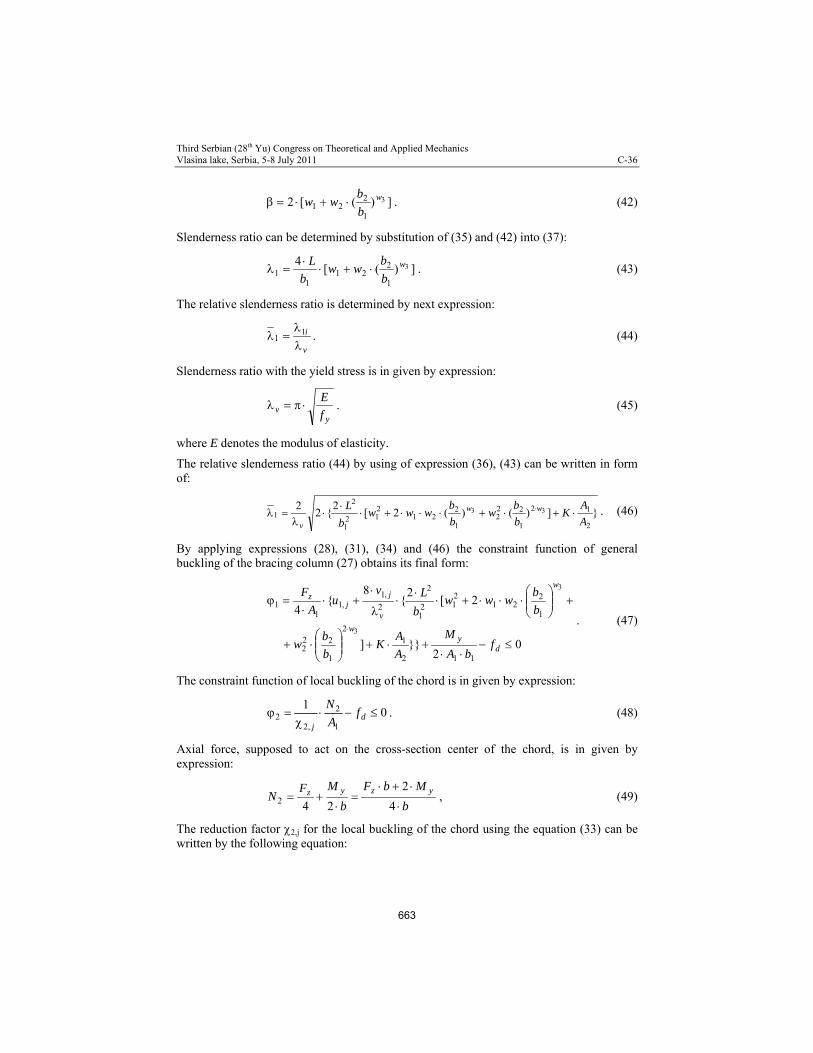
Third Serbian (28th Yu) Congress on Theoretical and Applied Mechanics Vlasina lake, Serbia, 5-8 July 2011 C-36
])([2 3
1
221
w
b
bww . (42)
Slenderness ratio can be determined by substitution of (35) and (42) into (37):
])([4 3
1
221
11
w
b
bww
b
L
. (43)
The relative slenderness ratio is determined by next expression:
v
i
11 . (44)
Slenderness ratio with the yield stress is in given by expression:
y
v f
E . (45)
where E denotes the modulus of elasticity.
The relative slenderness ratio (44) by using of expression (36), (43) can be written in form of:
}])()(2[2
{22
2
12
1
222
1
221
212
1
2
133
A
AK
b
bw
b
bwww
b
L ww
v
. (46)
By applying expressions (28), (31), (34) and (46) the constraint function of general buckling of the bracing column (27) obtains its final form:
02
}}]
2[2
{8
{4
112
12
1
222
1
221
212
1
2
2
,1,1
11
3
3
dy
w
w
v
jj
z
fbA
M
A
AK
b
bw
b
bwww
b
Lvu
A
F
. (47)
The constraint function of local buckling of the chord is in given by expression:
01
1
2
,22
d
j
fA
N. (48)
Axial force, supposed to act on the cross-section center of the chord, is in given by expression:
b
MbF
b
MFN
yzyz
4
2
242 , (49)
The reduction factor 2,j for the local buckling of the chord using the equation (33) can be written by the following equation:
663

Third Serbian (28th Yu) Congress on Theoretical and Applied Mechanics Vlasina lake, Serbia, 5-8 July 2011 C-36
22,1,1
,21
jj
jvu
. (50)
Least radius of gyration is in the form:
1
12 A
Ii y )1( 112 Ai . (51)
The slenderness ratio for a fixed ends beam and effective buckling length of chords 0.9ls [15] can be written in form of:
2
)1(2
9.0
i
ls )52(
11
)1(2
9.0
A
ls
. (52)
The relative slenderness ratio is determined by next expression:
v
2
2 )53( 11
)1(2
9.01
A
ls
v
. (53)
By application of the expressions (19) and (53) the reduction factor 2,j (50) finally becomes:
2
2
11
21
2,1
,1,2 )(
)1(81.01
tg
tg
A
bvu
v
jj
j
. (54)
Substitution of expressions (49) and (54) into Eq. (48) yields:
0])(
)1(81.0[
4
22
2
11
21
2
,1,1
12
d
v
jj
yzf
tg
tg
A
bvu
Ab
MbF. (55)
The constraint function of local buckling of the bracing diagonal is in given by expression:
01
2,33
d
d
j
fA
F. (56)
Axial force supposed to act on the cross-section center of the bracing diagonal is given by expression:
)sin(2
LqFF x
d )5( )cos(sin2
LqFF x
d . (57)
The reduction factor for the local buckling of the bracing diagonal using the equation (33) can be written in the following form:
23,3,3
,31
jj
jvu
. (58)
Least radius of gyration is in given by expression:
664

Third Serbian (28th Yu) Congress on Theoretical and Applied Mechanics Vlasina lake, Serbia, 5-8 July 2011 C-36
2
23 A
Ii y )1( 223 Ai . (59)
The slenderness ratio for a fixed ends beam and effective buckling length of bracings 0.75lr [15] is determined by next expression:
3
)1(3
75.0
i
lr )66,16( )sin(cos
)1(75.0
22
13
tgA
tgb. (60)
The relative slenderness ratio is determined by next expression:
v
3
3 . (61)
Substitution of expressions (60) and (61) into Eq. (58) yields:
22
222
221,3
,3,3 )sin(cos)(
)1(5625.01
tgA
tgbvu
v
jj
j
. (62)
By application of the expressions (57) and (62) the constraint function of local buckling of the bracing diagonal (56) becomes finally:
.0])sin(cos)(
)1(5625.0[
)cos(sin2
2222
2
221,3
,3
23
dv
jj
x
ftgA
tgbvu
A
LqF
(63)
I concluded that analytical solution of minimization of the objective function (26) could not be determined for model with previous constraint functions (47), (55) and (63). For this reason, the optimal parameters should be numerically determined.
5. Numerical Example and Analysis of Results
The verification of theoretical results is carried out on a numerical example for a lattice column with the following data: k1=0.05, L=30 m, =45O, fy=235 N/mm2, =1.504 (circular cross section).
The graphs of optimum parameters in the function of transverse force (Fx) for the lattice-columns with the overall dimensions of construction cross-section are unvarying along the construction were taken from paper [13].
By analyzing graphs (Fig. 2a) it can be concluded that the optimal height of the parallel chords on the bottom of construction (b1(II)) for unvarying shape lattice-columns is greater than the optimal height of the parallel chords for variable shape (b1(I)). Based on the analysis of Fig. 2 it may concluded that the optimal heights of the parallel chords on the
665

Third Serbian (28th Yu) Congress on Theoretical and Applied Mechanics Vlasina lake, Serbia, 5-8 July 2011 C-36
bottom and the top of construction have the same values in case of smaller values of the transverse force (Fx).
On the other hand, optimal cross-sectional area of one chord (A1(I)) for variable shape lattice-columns is greater than the optimal cross-sectional area of one chord (A1(II)) for unvarying shape.
Fig. 2. Change of optimum parameters in the function of transverse force (Fx) for variable (I) and unvarying (II) shape lattice-columns
6. Conclusion
The optimization of the bracing column against buckling was performed in this paper. The analysis was carried out based on buckling criterions: general buckling of the lattice column, local buckling of the chord and local buckling of the bracing diagonal. This paper’s objective is to determine optimal parameters of the variable shape lattice-columns. The optimal parameters were numerically determined. Obtained results are compared with the results that published in paper where goal was to determine optimal parameters of the unvarying shape lattice-columns.
Acknowledgement. The research work was supported by the Ministry of Science and Technological Development of the Republic of Serbia (Grant No. 36010).
666

Third Serbian (28th Yu) Congress on Theoretical and Applied Mechanics Vlasina lake, Serbia, 5-8 July 2011 C-36
References
[1] Andjelić N., Milošević-Mitić V., (2007), An approach to the optimization of thin-walled cantilever open
section beams, Theoretical and Applied Mechanics, Vol.34, No.4, pp. 323-340, Belgrade [2] Atanacković T., (1987), Teorija stabilnosti elastičnih štapova, FTN Novi Sad [3] Banichuk N. V., Ragnedda F. and Serra M., (2004), Optimum shapes of bar cross-sections, Structural
Multidisciplinary Optimization 23, 222–232 [4] Eurocode 3, (1992), Design of steel structures, CEN European Committee for Standardization, Brussels [5] Farkas J., (1984), Optimum design of metal structures, Akademiai KIADO, Budapest [6] Farkas J., Jármai K., (1997), Analysis and optimum design of metal structures, Rotterdam, Balkema [7] Farkas J., (2005), Structural optimization as a harmony of design, fabrication and economy, Structural
Multidisciplinary Optimization 30, 66–75 [8] Jarmai K., Farkas J., Optimum cost design of welded box beams with longitudinal stiffeners using advanced
backtrack method, Structural Multidisciplinary Optimization (2001) 21: 52-59 [9] Гохберг М.М., (1988), Справочник по кранам, Машиностроение, Ленинград [10] Kastratović G., Mijailović R., (2009), Optimum dimensions of trapezoid cross-section in lattice structures, 2nd
International Congress of Serbian Society of Mechanics (IConSSM 2009), Palić (Subotica), Serbia, pp. C-01:1-10
[11] Lanfeng Yu, (2008), Calculation method and control value of static stiffness of tower crane, Journal of Mechanical Science and Technology 22, pp. 829–834
[12] Mijailovic R., Kastratovic G., (2009), Cross-section optimization of tower crane lattice boom, Meccanica 44: 599–611
[13] Mijailović R., (2010), Optimum design of lattice-columns for buckling, Structural and Multidisciplinary Optimization, Volume 42, Number 6, pp. 897–906
[14] Petković Z., Ostrić D., (1996), Metalne konstrukcije u mašinogradnji, Institut za mehanizaciju Mašinskog fakulteta Univerziteta u Beogradu, Belgrade
[15] Rondal J., Wurker K.G., Dutta D., Wardenier J., Yeomans N., (1992), Structural Stability of Hollow Sections, Verlag TUV Rheinland, Koln, Germany
[16] Selmic R., Cvetkovic P., (1993), Determination of optimum dimension of lattice structure cross-sections, Facta Universitatis 3, 365–372
[17] Selmic R., Cvetkovic P., Mijailiovic R., Kastratovic G., (2006), Optimum Dimensions of triangular cross-section in lattice structures, Meccanica 41: 391–406
[18] Selmic R., Cvetkovic R., Mijailovic R., (2006), Optimization of cross-section in structures, monograph, The Faculty of Transport and Traffic Engineering, Belgrade
Radomir Mijailović works as an associate professor at the Faculty of Transport and Traffic Engineering in Belgrade, Serbia, where he earned his Ph.D. He is the author/co-author of more than 50 research papers. Research interests: dynamic modeling and optimization of cranes and vehicles, energy efficiency, end-of-life vehicle.
667

Third Serbian (28th Yu) Congress on Theoretical and Applied Mechanics Vlasina lake, Serbia, 5-8 July 2011 C-37
MATHEMATICAL MODELING OF FUNCTIONS DEPENDENCE OF FORCE – DEFORMATION IN A COLLISION OF VEHICLES
Radomir Mijailović Faculty of Transport and Traffic Engineering The University of Belgrade, Vojvode Stepe 305, 11000 Belgrade, Serbia e-mail: [email protected]
Abstract. Graph of dependence of force upon deformation is a commonly used graph in the field of the vehicle safety. The error present in determination of the modeling of preceding dependence has a considerable influence on the outcome results of the collision analysis. By comparative analysis of literature once can notice that the case of described previous dependences with two linear curves is often used (one for compression process and one for restitution process). By correlation analysis of experimental curves, we concluded that the previous approximation does not describe graph of dependence of force upon deformation with satisfactory way. This paper’s objective is mathematical modeling of functions dependence of force – deformation in a collision of vehicles. The compression process was approximated with piecewise linear functions with one and more than one regions. The restitution process may be approximated with linear functions. The quality of the coherence between experimental curves and mathematical functions is quantified by residual sum of squares.
Keywords: vehicle, crash, force, deflection, residual sum of squares.
1. Introduction
Determining the adequate functions dependence of force upon deformation of vehicles must to represent one of the major tasks in the analysis of impact of vehicles [1]. Their determination influence importantly on reduction of error in the output result of the analysis of impact process.
There are a few approaches in literature for defining the functions dependence of force – deformation of collisions vehicles. Usually mechanical-mathematical model presume that the curve dependence of force upon deformation can be described with two linear curves (one curve for compression process and one curve for restitution process) [2]. In this case force can be described in form of multiplication of deformation and appropriate stiffness. The difficulty lays in determining the stiffness during the processes of compression and restitution of vehicles. The approximate expression for the processes of compression may be found in the literature [3, 4], where is used vehicle mass (mv), impact velocity (v0) and its maximal deformation (max):
2max
20
vmc v . (1)
668

Third Serbian (28th Yu) Congress on Theoretical and Applied Mechanics Vlasina lake, Serbia, 5-8 July 2011 C-37
To my knowledge the analytical expression for strictly determination of stiffness during the restitution processes is not yet available. Usually in practical defining the previous stiffness is through usage of coefficient of restitution. What is the problem? Usually mechanical-mathematical models presume cognition of numeric values of coefficient of restitution. In practice, it is common that numerical value of coefficient of restitution is determined on basis of experience. The error present in determination of the value of coefficient of restitution has a considerable influence on the outcome results of the collision analysis and determination of stiffness during the processes of restitution.
The force deformation curves for the vehicle models can also be approximated as piecewise linear with three regions: before buckling has started, after buckling has started and when the occupant compartment starts to deform [5].
Elmarakbi and Zu [6] presume that the curve dependence of compression force upon deformation can be described using piecewise linear functions but with two regions.
Usually authors presume that the force has zero value at the moment when the appropriate deformation has zero value. However, there are other approaches to determining the functions dependence of force upon deformation of vehicles. McCoy and Lankarani [7] presume that the force have value greater than zero at the initial moment of vehicle's crush when the deformation has zero value.
The experimental data for the crash tests may be found in literature. Most of the tests were made at about 60 km/h [8, 9]. It also can be found papers [10, 11, 12] which presented the experimental data for the same vehicle at different impact velocity.
Based on currently published papers may be noticed necessity for defining new functions dependence of force upon deformation of vehicles.
This paper’s objective is to obtain new function that represent realistic behavior of vehicle during the impact. This function should be simple enough for practical implementation. We presume that the curve dependence of compression force upon deformation can be described using piecewise linear functions with three regions. Curves dependences for process of restitutions are approximated using linear functions with one and more than one regions. The stiffness during the process of restitution is expressed as function dependence of maximum vehicle deformation. Purpose of the model is reduction of error in the output results of the analysis of vehicle impact process.
2. The function dependence of force upon deformation
The function dependence of force upon deformation is determined by the following expression:
0
0
forF
forFF
r
k . (2)
2.1. The function dependence of compression force upon deformation
669

Third Serbian (28th Yu) Congress on Theoretical and Applied Mechanics Vlasina lake, Serbia, 5-8 July 2011 C-37
In this paper the function dependence of compression force upon deformation of vehicles is analyzed in view of correlation for piecewise linear functions with one and more than one regions (n regions) (Fig. 1).
Fig. 1. Dependence of compression force upon deformation
Function of dependence of compression force upon deformation is given by expression:
,)(...)(
......
)()(
)(
0
11121
322121
2111
1
21
321
21
1
,
nnn AAAnAAA
AAAAAA
AAAA
A
nk
forccc
forccc
forcc
forc
F (3)
where Fk – compression force, – deformation of vehicle, n – maximum value of deformations during process of compression (experimental
data), ci – coefficients of proportionality during process of compression (region ''i'').
Coefficient of proportionality (c1 for n=1) in literature is known as the coefficients of stiffness. Therefore, in the following text we will use notion stiffness for ci.
It is necessary to define following unknown parameters ci and A,i (i=1 ... n-1).
Experiment is necessary in order to mathematical modeling of functions dependence of force upon deformation. In that sense experiment consists of impact of vehicles into an absolutely rigid barrier. To gain a better output results experiment must be repeated for different values of impact velocity [5, 10, 11, 12].
The quality of the coherence between experimental curves and mathematical functions is quantified by residual sum of squares. Why was chosen just residual sum of squares? The function of dependence of compression force upon deformation done by the minimization
670

Third Serbian (28th Yu) Congress on Theoretical and Applied Mechanics Vlasina lake, Serbia, 5-8 July 2011 C-37
of a residual sum of squares also has minimum error using it in determination work during compression process. A minimal error in determining the work also results in a minimal error in determining coefficient of restitution.
Residual sum of squares (RSS) measures the deviations of experimental from their predicted values:
nk
iikik FFRSS
1
2exp,,, )( , (4)
where Fk,exp,i is the ith experimental value of the variable to be predicted, and Fk,i is the predicted value of Fk,exp,i.
The determination of unknown parameters was performed by the minimization of a residual sum of squares. We concluded that the analytical solution of minimization of the function (4) can’t be determined for n1 (3) by application of some optimization methods [13]. Therefore, the unknown parameters (ci, A,i) should be numerically determined.
2.2. The function dependence of restitution force upon deformation
Fig. 2. Dependence of restitution forces upon deformation (dash line – compression force; solid line – restitution forces)
The restitution process is significantly shorter than compression process.
By the author using more complex functions wouldn’t significantly reduce the error, but on the other hand would be more complicated. Therefore, the restitution process was approximated with linear curve (Fig. 2). Slopes of restitution lines are a function of maximum value of deformation during process of compression (Bm).
Functions of dependence of restitution force upon deformation are given by expression:
)()(, mm BmBkmr bFF , (5)
where Fr,m – restitution force, Bm – maximum value of deformations during process of compression,
671

Third Serbian (28th Yu) Congress on Theoretical and Applied Mechanics Vlasina lake, Serbia, 5-8 July 2011 C-37
bm – stiffness (coefficients of proportionality) during process of restitution for Bm.
Stiffness (bm) can be determined from the conditions: during restitution process work determined by experimental data (Ar,m,exp) is equal to work determines using approximate functions (5) (Ar,m,appr):
apprmrmr AA ,,exp,, . (6)
Numerical value of work Ar,m,exp can be determined by using experimental data for the same vehicle characteristics and for different values of impact velocities. The analysis output data are two numerical values: Bm and Ar,m,exp.
Numerical value of work Ar,m,appr is given in following form:
mC
mB
dFA mrapprmr ,,, . (7)
Deformation of vehicle in the instant of separation (Cm) may be determined from the condition:
0)(, mCmrF . (8)
The deformation Cm can be determined by substitution of (5) into (8):
m
BkBC b
Fm
mm
)( . (9)
Finally, stiffness bm can be determined by applying equations (5), (6), (7) and (9):
exp,,
2
2
)]([
mr
Bkm A
Fb m
. (10)
The stiffness bm depends on the deformation Cm (10). The final step of modeling may be correlation analysis between bm and Cm.
3. Numerical example and the analysis of results
The analysis of unknown parameters was performed using experimental data given in paper [11] where the results obtained through experimental analysis for Ford Escort. The experimental data from previous paper was derived using the case of direct central impact of vehicles into an absolutely rigid barrier.
Quality comparison between two piecewise linear functions with subsequent number of regions (i.e. n and n+1) may be presented by comparing their RSS relative discrepancy:
%,1001
11
i
iiinin RSS
RSSRSSRSS , (11)
672

Third Serbian (28th Yu) Congress on Theoretical and Applied Mechanics Vlasina lake, Serbia, 5-8 July 2011 C-37
%1.12221 nnRSS , %7.332 nnRSS , %1.043 nnRSS (12)
The relative discrepancies for n4 tend to zero.
The same calculation was used for comparing two functions with n=1 where stiffness obtained using equations (1) and (4):
%,100)1.(
)4.()1.()4.1.(1
Eq
EqEqEqEqn RSS
RSSRSSRSS , (13)
%4.11)4.1.(1 EqEqnRSS . (14)
The approximate expression for the compression stiffness (1) is often used in practice. By analysis of equations (12) and (14) it can be concluded that this expression hasn’t satisfactory results.
Therefore, we propose to use piecewise linear functions dependence of compression force upon deformation with three regions.
Fig. 3. Dependence of compression force upon deformation for Ford Escort (exp – experimental data, n=1...4 – approximations (Eq. 3)
Functions of dependence of compression force upon deformation (3) with n regions (n=1...4) and experimental data are presented in a Figure 3. By visual analysis of Figure 3 it can be also concluded that expression (3) for n=1 and n=2 doesn’t have satisfactory results.
Compression stiffness (ci) and deformation (A,i) for linear functions dependence of compression force upon deformation with three regions have following values:
.23.1,/38
,43.0,/299
,16.0,/1034
1
2
1
3
2
1
mmkNa
mmkNa
mmkNa
A
A
A
(15)
673
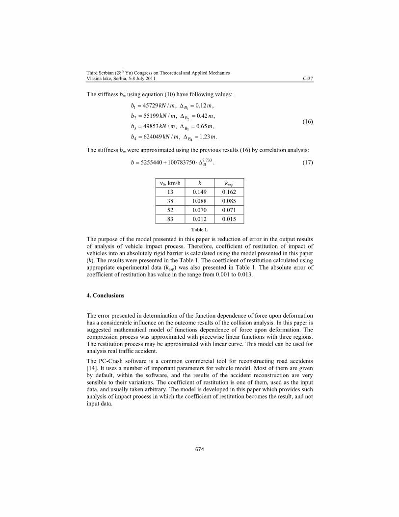
Third Serbian (28th Yu) Congress on Theoretical and Applied Mechanics Vlasina lake, Serbia, 5-8 July 2011 C-37
The stiffness bm using equation (10) have following values:
.23.1,/624049
,65.0,/49853
,42.0,/55199
,12.0,/45729
4
3
2
1
4
3
2
1
mmkNb
mmkNb
mmkNb
mmkNb
B
B
B
B
(16)
The stiffness bm were approximated using the previous results (16) by correlation analysis:
733.71007837505255440 Bb . (17)
v0, km/h k kexp
13 0.149 0.162
38 0.088 0.085
52 0.070 0.071
83 0.012 0.015
Table 1.
The purpose of the model presented in this paper is reduction of error in the output results of analysis of vehicle impact process. Therefore, coefficient of restitution of impact of vehicles into an absolutely rigid barrier is calculated using the model presented in this paper (k). The results were presented in the Table 1. The coefficient of restitution calculated using appropriate experimental data (kexp) was also presented in Table 1. The absolute error of coefficient of restitution has value in the range from 0.001 to 0.013.
4. Conclusions
The error presented in determination of the function dependence of force upon deformation has a considerable influence on the outcome results of the collision analysis. In this paper is suggested mathematical model of functions dependence of force upon deformation. The compression process was approximated with piecewise linear functions with three regions. The restitution process may be approximated with linear curve. This model can be used for analysis real traffic accident.
The PC-Crash software is a common commercial tool for reconstructing road accidents [14]. It uses a number of important parameters for vehicle model. Most of them are given by default, within the software, and the results of the accident reconstruction are very sensible to their variations. The coefficient of restitution is one of them, used as the input data, and usually taken arbitrary. The model is developed in this paper which provides such analysis of impact process in which the coefficient of restitution becomes the result, and not input data.
674

Third Serbian (28th Yu) Congress on Theoretical and Applied Mechanics Vlasina lake, Serbia, 5-8 July 2011 C-37
Further investigations may be directed towards establishing an analytical model for analysis of three dimensional vehicles collisions with the coefficient of restitution as the end result. Such analysis of collision processes would contribute to the analysis of traffic accidents.
Acknowledgement. The research work was supported by the Ministry of Science and Technological Development of the Republic of Serbia (Grant No. 36010).
References
[1] Harmati I.A., Rovid A., Varlaki P., Application of LPV Type Force Model in Vehicle Crash Dynamics,
Proceedings of the 9th WSEAS International Conference on Applications of computer engineering, 2010. [2] Pawlus W., Karimi H.R., Robbersmyr K.G., Mathematical modeling of a vehicle crash test based on elasto-
plastic unloading scenarios of spring-mass models, The International Journal of Advanced Manufacturing Technology, in press
[3] Janković A, Simić D, Vehicle safety, monograph, DSP-mecatronic, Kragujevac, 1996. [4] Nusholtz, G.S., Xu L., Shi Y., Domenico L.D., Vehicle mass, stiffness and their relationship, 19th ESV, Paper
number 05-0413, 2005. [5] Van der Zweep C.D., Jenefeldt F., Thomson R., Van der Zweep C.D., Jenefeldt F., Thomson R., 2002.
Improvement of vehicle crash compatibility through the development of crash test procedure, Project number – GRD2-2001-50083, 1998-2002., Project number – GRD2-2001-50083, 1998-2002.
[6] Elmarakbi A., Zu J., Mathematical modelling of a vehicle crash with emphasis on the dynamic response analysis of extendable cubic nonlinear dampers using the incremental harmonic balance method, Proc. IMechE Vol. 221 Part D: J. Automobile Engineering, pp. 143 – 156, 2007
[7] McCoy M.L., Lankarani H.M., Determination of the crush stiffness coefficients of a typical aftermarket frontal protective guard used in light trucks and vans with comparisons between guard stiffness and frontal vehicle crush coefficients, Proceedings of the Institution of Mechanical Engineers, Part D: Journal of Automobile Engineering, Vol. 220, 2006, pp. 1073 – 1084
[8] www.nhtsa.dot.gov [9] Huibers J., de Beer E., Curent front stiffness of European vehicles with regard to compatibility, International
Technical Conference on the Enhanced Safety of Vehicles (ESV), Amsterdam, The Netherlands, June 4 - 7, 2001.
[10] Kerkhoff JF, Husher SE, Varat MS, Busenga AM, Hamilton K, An investigation into vehicle Frontal impact stiffness, BEV and repeated testing for reconstruction, Society of Automotive Engineers International Congress, Detroit, Michigan, 1993, SAE Paper 930899
[11] Steffan H., Geigl B. C., Moser A., Hoschopf H., Comparison of 10 to 100 km/h rigid barrier impacts, Paper No. 98-S3-P-12
[12] Varat M. S., Husher S. E., Vehicle impact response analysis through the use of acceleration data, SAE Tech. Paper 2000-01-0850, 2000.
[13] Selmic R., Cvetkovic R., Mijailovic R., (2006), Optimization of cross-section in structures, monograph, The Faculty of Transport and Traffic Engineering, Belgrade
[14] Depriester JP, Perrin C, Serre T, Chalandon S., Comparision of several methods for real pedestrian accident, 2006, http://www.mathlab.mtu.edu/~struther/Drop/Modeling/05-0333-O.pdf
Radomir Mijailović works as an associate professor at the Faculty of Transport and Traffic Engineering in Belgrade, Serbia, where he earned his Ph.D. He is the author/co-author of more than 50 research papers. Research interests: dynamic modeling and optimization of cranes and vehicles, energy efficiency, end-of-life vehicle.
675

Third Serbian (28th Yu) Congress on Theoretical and Applied Mechanics Vlasina lake, Serbia, 5-8 July 2011 C-39
BENDING OF A THIN PLATE SUBJECTED TO STRONG UNIFORM MAGNETIC FIELD
V. Milošević-Mitić, T. Maneski, N. Anđelić
Faculty of Mechanical Engineering,
University of Belgrade, Kraljice Marije 16, 11120 Belgrade 35
e-mail: [email protected]
Abstract. The problem of an elastic plate, originally unmagnetized, in a uniform magnetic field is considered in the paper. The magnetic forces are of two kinds: the force of the magnetic field on conducting currents in the material, induced by its motion in the static field and the force between the magnetic field and the magnetized material (independent of the motion).The general equations are linearized by assuming linear constitutive equations and that all electromagnetic variables in the deformed body may be divided into two parts: a rigid body state and a perturbation state. Maxwell’s stress is calculated and involved in differential equation related to bending. Obtained equation is solved in analytical form using the integral-transformation technique (Double Fourier finite-sine transformation and Laplace transformation). Discussion of the obtained solution is done using Kirchhoff’s hypothesis.
1. Introduction
The theory of electro-magneto-thermoelasticity investigates the interaction between the straian and the electromagnetic field in a solid elastic body. A propagation of an elastic field in presence of magnetic field was considered by L. Knopoff (1955), J.W. Dunkin i A.C. Eringen (1963). F.W. Brown (1966) developed a rigorous phenomenological theory for ferromagnetic materials on the basis of the large deformation theory and the clasical theory of feromagnetisam. H.F. Tiersten (1964) developed an analogous theory based on a microscopic model. Since the general nonlinear theory is complicated, Y.W. Pao and C.S. Yeh 1 derived a set of linear equations and boundary conditions for soft feromagnetic elastic materials. They applied linear theory to investigate magnetoelastic buckling of an isotropic plate. The same problem was treated on the other way by F.C. Moon i Y.H. Pao 2. Basic general information about the theory of magneto-thermoelasticity was presented in monographs by H. Parkus 3. A great contribution of a research in this scientific field was given by W. Nowacki, S.A. Ambarcumian 4, M. Krakowski 5. From 1975 on Michigan Technological University (N.S. Christopherson, M.O. Peach, J.M. Dalrymple, L.G. Viegelahn 6), a set of experiments were done to reconsider theoretical results. Because of a disagreement in analytical and experimental results methods of numerical analyses were involved in consideration (K. Miya, T. Takagi, Y. Ando (1980), X. Tian and Y. Shen 7). Sharma and Pal investigated the propagation of magnetic-thermoelastic plane
676

Third Serbian (28th Yu) Congress on Theoretical and Applied Mechanics Vlasina lake, Serbia, 5-8 July 2011 C-39
wave in homogeneous isotropic conducting plate under uniform static magnetic field [8]. The problem with high-frequncy electromagnetic waves was presented in [9] and the problem with low-frequency electromagnetic field was descused in [10].
2. Basic equations
Electro-magneto-thermoelastic problem considered in the paper shows one type of interaction between electromagnetic and strain field in a solid plate. It is assumed that the plate material is elastic and isotropic, possessing a good electric conductivity. Many nickel-iron alloys used for building the magnetic circuits of motors, generators, inductors, transformers are of this type.
As a result of time changing electromagnetic field conducting currents appear in electric conductors. This problem is mathematically described by the system of Maxwell’s equations with the relations for slowly moving media and modified Ohm’s low 6:
t
DJHrot
, t
BKrot
,
0Ddiv
, 0Bdiv
, (1)
BuKD
0 , DuHB
,
BuKJ
,
where the following notation is applied: H – intensity of the magnetic field, K – intensity of the electric field, B – magnetic flux density (magnetic induction), D – electric induction, J – current density, u – deflection, 0 – permeability of vacuum, – electric conductivity, 0 – dielectric constant of vacuum, t – time.
In the consideration of the plate vibrations, we shall take the assumption that the longitudinal vibrations are independent of transversal vibrations. Transversal vibrations can be obtained by using the following differential equation 11:
3333333333
341 212 ii
ix
hTTw
hwhwD
2
2
33
2
2
33,,332
h
h
h
hiiiiii
i
dxXdxxfXTTx
h, (i=1,2), (2)
where: D – flexural rigidity of the plate, X – mechanical force, f – Lorenz force. ij and Tij denote mechanical and magnetic stress tensors (ij
+, Tij+ are stress components on the upper
and ij-, Tij
- on the lower side of the plate), where h is the plate thickness and is the
four-dimension Laplace operator.
41
Of course, presented systems of equations has to be accomplished with the appropriate set of boundary and initial conditions.
677

Third Serbian (28th Yu) Congress on Theoretical and Applied Mechanics Vlasina lake, Serbia, 5-8 July 2011 C-39
Presented system of differential equations is complicated to be solved in analytical form. So, at first we have to simplify mathematical model of the discusted problem. In this paper only the problem of the plate subjected to homogenius magnetic field will be presented.
In this case, electromagnetic energy which is converting in thermal energy is very small, so Joules heat can be neglected. Mahwell’s equations (1) can be linearysed, too. Deformation field is coupled with the magnetic field.
3. Thin metallic plate in a stationary homogenius magnetic field
Let the thin simply supported plate made of homogenius, isotropic linear magnetic material is subjected transversal to an external uniform homogenius magnetic field induction
000 HB
in air. The magnetic permeability of the plate material is =0r and at the
beginning the plate is quite non-magnetized (Figure 1).
x1
x2
x3
a
b
h
Figure1. Coordinate system and plate dimensions
In that case we have two kinds of forces:
1. forces of interaction between magnetic field and magnetized material, independent of vibrations - motion and
2. forces of the magnetic field and the conducting currents in the plate material, induced by the plate vibrations in the stationary magnetic field.
Electromagnetic field forming in the plate appeares on the action of magnetized material and macroscopic conducting current, as can be presented in next way
210 pppp hhHH
, (3)
where 1ph
and 2ph
are small fluctuations of the magnetic field generated on the presented
actions. In the mathematical model their influence on each other can be neglected.
If the thin metallic plate is placed in strong homogeneous magnetic field H0=const. appropriate of the law of the line refraction, in the plate is forming magnetic field intensity Hp0. In the moment t=0 plate is losing stability place, apropos the plate has initial deformation conditions. It can be presented in the next form
678

Third Serbian (28th Yu) Congress on Theoretical and Applied Mechanics Vlasina lake, Serbia, 5-8 July 2011 C-39
21021 ,0,, xxxxw , 211
0
21 ,,,
xxt
txxw
t
. (4)
On the coupling between the electromagnetic field and the deformation field there are small
fluctuations of the electric field e
and the magnetic field in the plate 2ph
, defined as
txxxhHtxxxH ppop ,,,,,, 3212
321
, (5)
txetxK ,,
.
As the change of the magnetic field under a deformation is small, for ferromagnetic materials can be accepted that the magnetic permeability is nearly constant const.. Neglecting of the productions between the values hpi
2, ei , vi and the productions of their derivatives, relations (1) have the next form 6
0pHveD
, 20 pp hHB
,
0pHveJ
, (6)
and the Maxwell’s equations are
002
ppp HveHvehrot
, 2pherot
,
00 pHvdivediv
, 02 phdiv
. (7)
Lorient’s force has a form
02
pp HDhrotBJf
. (8)
By eliminating value we can form differential equation for the magnetic field 6 as e
002222
1 ppppp HvrotHvrothhh
. (9)
In the case of the quazistationry electromagnetic field we have 0D
, 0
t
D
, or 0, so
presented equations have simplified form
02
pp Hhrotf
, (10)
022
1 ppt Huroth
. (11)
The whole equation system of this coupled magnetoelastic bending problem is consisted of the equations (11) and (2) together with the appropriate boundary and initial conditions and relation (10).
Let us discus one special case when the magnetic field is transversal to the middle surface of the thin plate. The plate is rectangular with the material density (Figure 1.). Using the
679
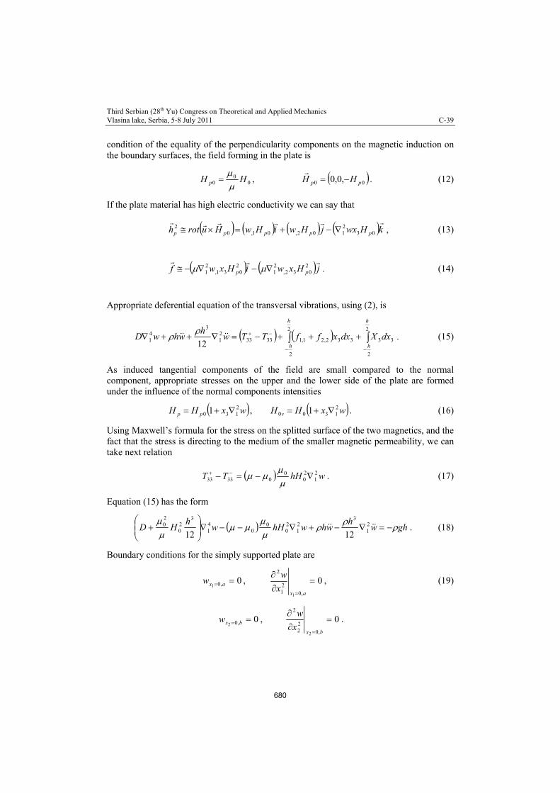
Third Serbian (28th Yu) Congress on Theoretical and Applied Mechanics Vlasina lake, Serbia, 5-8 July 2011 C-39
condition of the equality of the perpendicularity components on the magnetic induction on the boundary surfaces, the field forming in the plate is
00
0 HH p
, 00 ,0,0 pp HH
. (12)
If the plate material has high electric conductivity we can say that
kHwxjHwiHwHuroth ppppp
03
2102,01,0
2 , (13)
jHxwiHxwf pp
2
032,21
2031,
21 . (14)
Appropriate deferential equation of the transversal vibrations, using (2), is
2
2
33
2
2
332,21,1333321
341 12
h
h
h
h
dxXdxxffTTwh
whwD . (15)
As induced tangential components of the field are small compared to the normal component, appropriate stresses on the upper and the lower side of the plate are formed under the influence of the normal components intensities
wxHH pp2130 1 , wxHH v
21300 1 . (16)
Using Maxwell’s formula for the stress on the splitted surface of the two magnetics, and the fact that the stress is directing to the medium of the smaller magnetic permeability, we can take next relation
whHTT 21
20
003333
. (17)
Equation (15) has the form
ghwh
whwhHwh
HD
2
1
321
20
00
41
320
20
1212. (18)
Boundary conditions for the simply supported plate are
0w ,01 ax , 0,0
21
2
1
axx
w, (19)
0,02 bxw , 0
,0
22
2
2
bxx
w.
680

Third Serbian (28th Yu) Congress on Theoretical and Applied Mechanics Vlasina lake, Serbia, 5-8 July 2011 C-39
System of the equations (18) and (19) with the initial conditions (4) can be solved using integral transform technique – double sine Fourier transformation and the Laplace transformation. Obtained solution has next form
...5,3,1,2121 sinsin
4,,
nmmnmn xxtw
abtxxw ,
222
310
cos1
12
4sincos
nm
nm
mnmnnm
nmnmnmnmmn
t
hh
ghtttw
,
223
2220
00
2223
20
20
2
12
12
mn
mnmn
nmh
h
hHh
HD
,
a
nn
, b
mm
, (20)
a b
mnkknm dxdxxxxx0 0
212121 sinsin, (k=0,1).
4. The conclusion
The analysis of the obtained results can be done using relation for nm. In the cases of the paramagnetics and ferromagnetics we have (-0)>0 and the magnetic field is acting in the same direction of the elastic field. It means that the magnetic field is in corelation with the elasic field and they together gravity to return the plate in the equilibrium position. For diamagnetic materials we have (-0)<0 and the magnetic field is acting in opposite direction of the direction of the elastic field.
Using relation (17) and Kirchoff hypothesis, on the base of a sign of , we have to
conclude that in the case of the plate clamped on only one side we have opposite situation.
w21
681
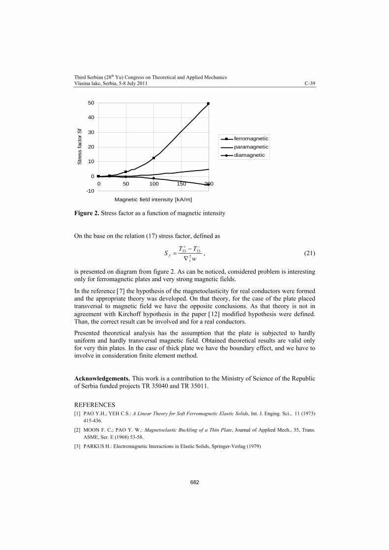
Third Serbian (28th Yu) Congress on Theoretical and Applied Mechanics Vlasina lake, Serbia, 5-8 July 2011 C-39
-10
0
10
20
30
40
50
0 50 100 150 200
Magnetic field intensity [kA/m]
Stres
s fa
ctor
Sf
ferromagnetic
paramagnetic
diamagnetic
Figure 2. Stress factor as a function of magnetic intensity
On the base on the relation (17) stress factor, defined as
w
TTS f 2
1
3333
, (21)
is presented on diagram from figure 2. As can be noticed, considered problem is interesting only for ferromagnetic plates and very strong magnetic fields.
In the reference 7 the hypothesis of the magnetoelasticity for real conductors were formed and the appropriate theory was developed. On that theory, for the case of the plate placed transversal to magnetic field we have the opposite conclusions. As that theory is not in agreement with Kirchoff hypothesis in the paper 12 modified hypothesis were defined. Than, the correct result can be involved and for a real conductors.
Presented theoretical analysis has the assumption that the plate is subjected to hardly uniform and hardly transversal magnetic field. Obtained theoretical results are valid only for very thin plates. In the case of thick plate we have the boundary effect, and we have to involve in consideration finite element method.
Acknowledgements. This work is a contribution to the Ministry of Science of the Republic of Serbia funded projects TR 35040 and TR 35011.
REFERENCES [1] PAO Y.H.; YEH C.S.: A Linear Theory for Soft Ferromagnetic Elastic Solids, Int. J. Enging. Sci., 11 (1973)
415-436.
[2] MOON F. C.; PAO Y. W.: Magnetoelastic Buckling of a Thin Plate, Journal of Applied Mech., 35, Trans. ASME, Ser. E (1968) 53-58.
[3] PARKUS H.: Electromagnetic Interactions in Elastic Solids, Springer-Verlag (1979)
682

Third Serbian (28th Yu) Congress on Theoretical and Applied Mechanics Vlasina lake, Serbia, 5-8 July 2011 C-39
[4] AMBARCUMIAN S.A.; BAGDASARIAN G.E.; BIELUBIEKIAN M.V.: Magnetoelasticity of Thin Shells
and Plates [in Russian], Nauka, Moscow (1977)
[5] KRAKOWSKI M.: Mathematical Model of Eddy Currents in a Metallic Solid after Applying an External Magnetic Field, Bullet. of the Polish Acad. of Science, 29, No. 5-6, Varsaw (1981) 67-71.
[6] PEACH M.O.; CHRISTOPHERSON N.S.; DALRYMPLE J.M.; VIEGELAHN G. L.: Magnetoelastic Buckling: Why Theory and Experiment Disagree, Experimental Mech., 28, No 1 (1988) 65-69.
[7] TIAN X.; SHEN Y.: Generalized magneto-thermoelasticity solved by FEM in time domain, Springer, Comput. Methods (2006) 1621-1627.
[8] SHARMA J.N.; PAL M.: Rayleigh-Lamb waves in magneto-thermoelastic homogeneous isotropic plate, Int. J. of Eng. Sci. 42 (2004) 137-155.
[9] Miloševic-Mitić V, Kozak D, Maneski T, Anđelić N, Gaćeša B, Stojkov M, Dynamic nonlinear temperature field in a ferromagnetic plate induced by high frequency electromagnetic waves, Strojarstvo Vol. 52, No. 2 (2010) 115-124
[10] Milošević-Mitić V, Maneski T, Temperature Loading of a Thin Metallic Plate Subjected Transversal to Law-Frequency Electromagnetic Field, FME TRANSACTIONS, Vol 38, No. 2 (2010) 95-101
[11] MILOŠEVIĆ-MITIĆ V. Magneto-thermo-elastic bending of thin plates; Monogr., Zadužbina Andrejević, Belgrade (1999)
[12] Rudnicki M, A Modified Hypothesis of magnetoelasticity of Plates, Bull. of the Polish Academy of Sciences, Vol. 32, no 3-4, (1984) 101-112
683

Third Serbian (28th Yu) Congress on Theoretical and Applied MechanicsVlasina Lake, Serbia, 5-8 July 2011
SOME QUADRATURE RULES FOR FINITE ELEMENT METHODAND BOUNDARY ELEMEN T METHOD
G.V. Milovanovi c1, T. Igi c2, N. Toncev2
1 Faculty of Computer Sciences, Megatrend University, Bulevar Umetnosti 29, 11070 NoviBeograd, Serbiae-mail: [email protected] Faculty of Civil Engineering and Architecture, University of Niš, A. Medvedeva 14, 18000Niš, Serbiae-mail: [email protected]
Abstract. The boundary element method (BEM) and the f nite element method (FEM) arevery popular in many computational applications in engineering. These methods very oftenrequire the numerical evaluation of one dimensional or multiple integrals with singular ornear singular integrands. Such problems appear in many subjects of mechanics (fracturemechanics, damage mechanics, etc.), as well as in other technical f elds. In this paper wegive some improvements of quadrature rules for FEM and BEM. Beside of general notions onGaussian quadratures, we give a construction of weighted Gaussian quadratures for integralswith logarithmic and/or algebraic singularities. Also, we consider generalized quadratures ofhigh degree of precision for Müntz systems. Numerical examples are included.
1. Introduction
The boundary element method (BEM) and the f nite element method (FEM) are very popularin many computational applications in engineering, for example, in fracture mechanics,damage mechanics, electromagnetic diffraction, etc. Very often in such applications weneed accurate numerical evaluation of one dimensional or multiple integrals with singularkernels and/or singular basis functions. Two kinds of singularities are typical: algebraicand logarithmic. Müntz and Müntz-logarithmic polynomials are typical functions with suchproperties. Also, an accurate evaluation of nearly singular one and multidimensional integralsis very important. For some additional details see, for example, [1], [9], [7], [8], [10], [11],[17], [18].
In this paper we propose a method for constructing the weighted Gaussian quadraturerules for integrals with algebraic and/or logarithmic singularities. This method gives Gaussianquadratures with a maximal algebraic degree of precision. Also, we mention anotherapproach which enables us to obtain Gaussian quadratures for Müntz systems (for detailssee Milovanovic [13] and Milovanovic and Cvetkovic [15]).
Beside of general notions on quadratures of high algebraic degree of precision, weconsider a stable and eff cient construction of the weighted Gaussian quadratures for integralsof functions with end-point singularities. Such a construction is based on an application ofthe Mathematicapackage OrthogonalPolynomials, recently developed by Cvetkovic andMilovanovic [2]. Numerical examples are included.
684

2. Quadrature Formulas for Integrals With Logarithmic Weight Functions
In numerical implementation of the BEM (see [9, Chapters 4 & 5]), quadrature formulasplay a very important role, especially for higher order elements. For calculating integrals ofthe corresponding inf uence coeff cients (for off-diagonal elements and diagonal elements),quadratures of Gaussian type are very appropriate. For suff ciently smooth functions on af nite interval [a,b] a linear transformation to the standard interval [−1,1] can be used andthen an application of Gauss-Legendre quadrature formula provides numerical integrationwith a satisfactory accuracy. However, for integrals with a logaritmic singularity and/or somekind of algebraic singularities the convergence of the corresponding quadrature process isvery slow, so that certain weighted quadratures are recommended. In such cases, the weightfunctions of the corresponding weighted Gaussian quadratures include these “diff cult parts(with singularities)” of the integrand. In this section, we consider a few cases of suchquadratures on the standard interval [0,1]. However, we f rst give some general notions onGaussian quadratures.
2.1. General notions of Gaussian quadratures
Let Pm be a set of all algebraic polynomials of degree at most m. We consider the n-pointweighted quadrature formula
∫ b
af (x)w(x)dx=
n
∑k=1
Ak f (xk)+Rn( f ), (1)
where the weight function w(x) is such one that all its moments µk =∫ b
a xkw(x)dx < +∞,k = 0,1, . . ., and µ0 > 0. Quadrature rule (1) is known as interpolatoryif it is exact for allpolynomials of degree at least n−1, i.e., if the remainder term Rn( f ) = 0 for each f ∈Pn−1.
However, if the nodes xk and the weights Ak in (1) are selected so that Rn( f ) = 0 foreach f ∈ P2n−1, the rule (1) is the Gaussianquadrature formula. In that case, the nodesxk are zeros of the monic orthogonal polynomial πn(w;x) and the corresponding weights Ak
(Christoffel numbers) can be expressed by the so-called Christoffel function λn(w;x) (cf.[12, Chapters 2 & 5]) in the form Ak = λn(w;xk) > 0, k = 1, . . . ,n. Positivity of Christoffelnumbers is very important for the convergence of the quadrature formulas. In the specialcase w(x) = 1 on [−1,1], the nodes xk are zeros of the Legendre polynomial Pn(x). It wasoriginally discovered by Gauss in 1814, of course, without theory of orthogonality.
As we know [12, Chapters 2], the (monic) polynomials πn(w;x) orthogonal with respectto the weight function w(x) on [a,b] satisfy the three-term recurrence equation
πk+1(t) = (t −αk)πk(t)−βkπk−1(t), k = 0,1,2, . . . , (2)
π0(t) = 0, π−1(t) = 0,
where (αk) = (αk(w)) and (βk) = (βk(w)) are sequences of recursion coeff cients. Thecoeff cient β0 which is multiplied by π−1(x) = 0 in the recurrence relation (2) may bearbitrary, but it is convenient to def ne it by β0 = µ0 =
∫ ba w(x)dx.
For generating Gaussian quadrature rules there are numerical methods, which arecomputationally much better than a computation of nodes by using Newton’s method and thena direct application of the classical Christoffel’s expressions for the weights (see e.g. Davis
685

and Rabinowitz [3]). The characterization of the Gaussian quadratures via an eigenvalueproblem for the Jacobi matrix
Jn(w) =
α0√
β1 O√
β1 α1√
β2√
β2 α2. . .
. . . . . .√
βn−1O
√
βn−1 αn−1
(3)
has become the basis of current methods for generating these quadratures. The most popularof them is one due to Golub and Welsch [6]. Their method is based on determining theeigenvalues and the f rst components of the eigenvectors of a symmetric tridiagonal Jacobimatrix (3), where αν and βν , ν = 0,1, . . . ,n− 1, are the coeff cients in the three-termrecurrence relation (2) for the monic orthogonal polynomials πν(w; ·). Namely, the nodes xkin the Gaussian quadrature rule(1), with respect to the weight function w(x) on [a,b], arethe eigenvalues of the n-th order Jacobi matrix(3). The weights Ak are given by
Ak = β0v2k,1, k = 1, . . . ,n,
whereβ0 = µ0 =∫ b
a w(x)dx and vk,1 is the first component of the normalized eigenvectorvk
corresponding to the eigenvalue xk,
Jn(w)vk = xkvk, vTk vk = 1, k = 1, . . . ,n.
Simplifying QR algorithm so that only the f rst components of the eigenvectors arecomputed, Golub and Welsch [6] gave an eff cient procedure for constructing the Gaussianquadrature rules. This procedure was implemented in several programming packagesincluding our package OrthogonalPolynomials realized in Mathematica [2].
Thus, we need the recursion coeff cients αk and βk, k≤N−1, for the monic polynomialsπν(w; ·), in order to construct the n-point Gauss-Christofell quadrature formula, with respectto the weighte w(x), for each n ≤ N. These coeff cients are known explicitly for theclassical orthogonal polynomials (see [12, Chapters 2]). In other cases we need an additionalnumerical construction of recursion coeff cients, using the method of moments or the so-called discretized Stieltjes procedure (see [12, § 2.4.8]).
2.2. Gaussian formulas for the weight w(x) = (1−x)αxβ log(1/x)
We consider the n-point quadrature formula∫ 1
0f (x)(1−x)αxβ log
1x
dx=n
∑k=1
Ak f (xk)+Rn( f ), (4)
with parameters α,β > −1 in the weight function w(x) = (1− x)α xβ log(1/x). Piessensand Branders [19] considered cases when α = 0 and β = 0,±1/2,±1/3,−1/4,−1/5 (seealso Gautschi [4] and [5]). Quadrature parameters for n ≤ 8 was given in Katsikadelis [9,pp. 297–298] in the case α = β = 0.
Using symbolic integration we f nd the moments µk = µk(α,β ) in terms of the gammafunction and harmonic numbers,
µk(α,β ) =
∫ 1
0xkw(x)dx=
∫ 1
0(1−x)αxk+β log
1x
dx
686

=Γ(α + 1)Γ(β +k+ 1)
Γ(α + β +k+ 2)[H(α + β +k+ 1)−H(β +k)] . (5)
For example, for α = β = 0 it reduces to µk(0,0) = 1/(k+ 1)2, k≥ 0.The standard meaning of the k-th harmonic number Hk is the sum of the reciprocals of
the f rst k natural numbers, i.e.,
Hk = H(k) =k
∑ν=1
1ν
,
and its representation is given by Euler in the form
H(k) =
∫ 1
0
1− tk
1− tdt =
k
∑ν=1
(−1)ν−1 1ν
( kν
)
.
Taking a fractional argument x between 0 and 1, the harmonic number H(x) is def nedby the previous integral, where k is simply replaced by x. Then it can be generated byH(x) = H(x−1)+x−1 or
H(1−x)−H(x) = π cot(πx)− 1x
+1
1−x.
More generally, for every x > 0 (integer or not), the harmonic number is determined by
H(x) = x+∞
∑k=1
1k(x+k)
= ψ(x+ 1)+ γ,
where ψ(x) = Γ′(x)/Γ(x) is the so-called digammafunction, i.e., the logarithmic derivative ofthe gamma function Γ(x) and γ = 0.577215664901532 . . . is the Euler-Mascheroni constant.
Using the Mathematica package OrthogonalPolynomials [2] and the f rst 2Nmoments µk, k = 0,1, . . . ,2N− 1, given by (5), we get the f rst N coeff cients αk and βk,k= 0,1, . . . ,N−1, in the recurrence relation (2). It enables us to obtain quadrature parametersin (4) for any n≤ N.
Remark. In order to overcome the severe ill-conditioning in obtaining the recursioncoeff cients with a satisfactory accuracy, a multi-precision arithmetic can be used. Forexample, in the simplest case α = β = 0, taking 55-decimal-digit arithmetic we get the f rstN = 50 recursion coeff cients to about 20 decimal digits.
The following code in the Mathematica package OrthogonalPolynomials [2]generates recursion coeff cients for k ≤ 2N− 1 = 99 and quadrature parameters (nodes andweights) to 20 decimal digits for n = 10(10)50:
In[1]:= << orthogonalPolynomials`
In[2]:= w@t_, a_, b_ D := H1 - tL ^a t^b Log@ 1 � tD
In[3]:= mom= Integrate @t ^k w @t, 0, 0D, 8t, 0, 1<D; moments = Table@ mom, 8k, 0, 99<D;
In[4]:= 8alpha, beta< = aChebyshevAlgorithm @moments, WorkingPrecision ® 55D;
In[5]:= param = Table@aGaussianNodesWeights @n, alpha, beta,Precision ® 20, WorkingPrecision ® 20D, 8n, 10, 50, 10<D;
For example, the obtained nodes and weights for n = 10 are given in the following list:
687
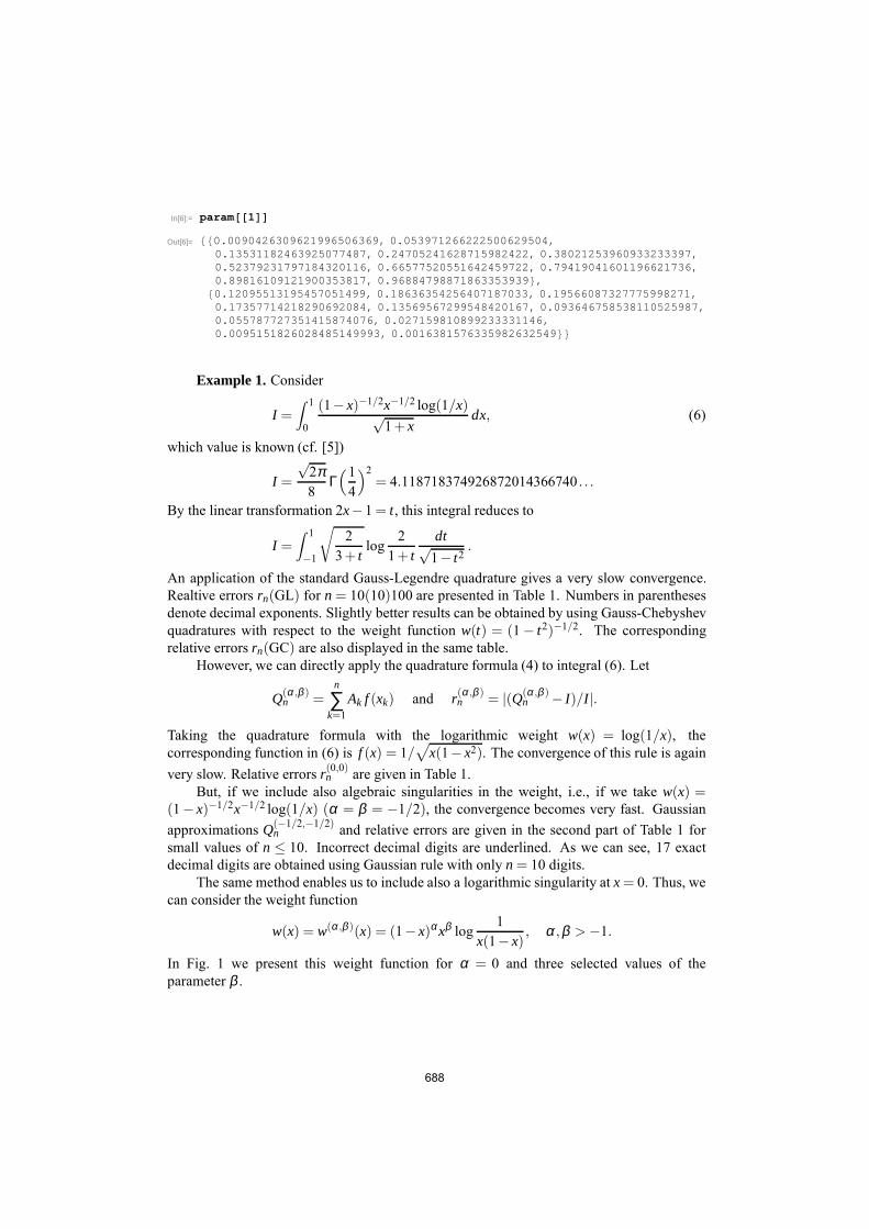
In[6]:= param@@1DD
Out[6]= 880.0090426309621996506369, 0.053971266222500629504,0.13531182463925077487, 0.24705241628715982422, 0.38021253960933233397,0.52379231797184320116, 0.66577520551642459722, 0.79419041601196621736,0.89816109121900353817, 0.96884798871863353939<,80.12095513195457051499, 0.18636354256407187033, 0.19566087327775998271,0.17357714218290692084, 0.13569567299548420167, 0.093646758538110525987,0.055787727351415874076, 0.027159810899233331146,0.0095151826028485149993, 0.0016381576335982632549<<
Example 1.Consider
I =∫ 1
0
(1−x)−1/2x−1/2 log(1/x)√1 +x
dx, (6)
which value is known (cf. [5])
I =
√2π8
Γ(1
4
)2= 4.118718374926872014366740 . . .
By the linear transformation 2x−1 = t, this integral reduces to
I =∫ 1
−1
√
23 + t
log2
1 + tdt√
1− t2.
An application of the standard Gauss-Legendre quadrature gives a very slow convergence.Realtive errors rn(GL) for n = 10(10)100 are presented in Table 1. Numbers in parenthesesdenote decimal exponents. Slightly better results can be obtained by using Gauss-Chebyshevquadratures with respect to the weight function w(t) = (1 − t2)−1/2. The correspondingrelative errors rn(GC) are also displayed in the same table.
However, we can directly apply the quadrature formula (4) to integral (6). Let
Q(α ,β )n =
n
∑k=1
Ak f (xk) and r(α ,β )n = |(Q(α ,β )
n − I)/I |.
Taking the quadrature formula with the logarithmic weight w(x) = log(1/x), thecorresponding function in (6) is f (x) = 1/
√
x(1−x2). The convergence of this rule is againvery slow. Relative errors r(0,0)
n are given in Table 1.But, if we include also algebraic singularities in the weight, i.e., if we take w(x) =
(1− x)−1/2x−1/2 log(1/x) (α = β = −1/2), the convergence becomes very fast. Gaussianapproximations Q(−1/2,−1/2)
n and relative errors are given in the second part of Table 1 forsmall values of n ≤ 10. Incorrect decimal digits are underlined. As we can see, 17 exactdecimal digits are obtained using Gaussian rule with only n = 10 digits.
The same method enables us to include also a logarithmic singularity at x= 0. Thus, wecan consider the weight function
w(x) = w(α ,β )(x) = (1−x)αxβ log1
x(1−x), α,β > −1.
In Fig. 1 we present this weight function for α = 0 and three selected values of theparameter β .
688
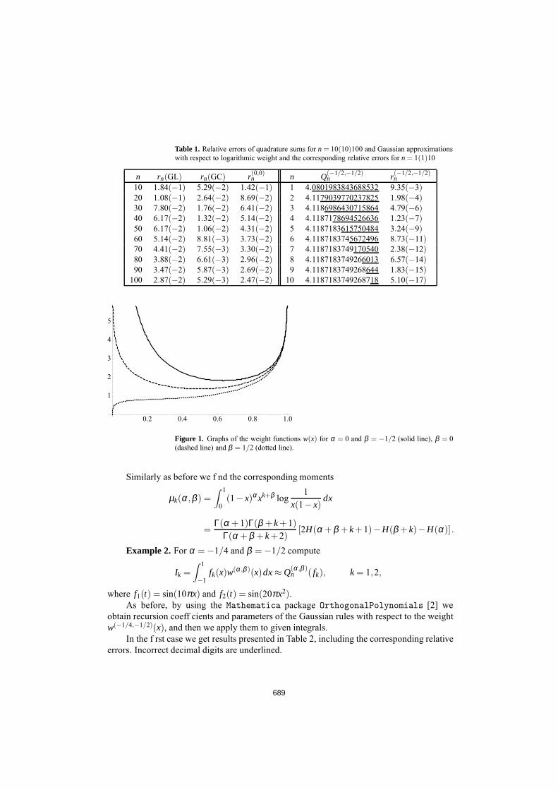
Table 1. Relative errors of quadrature sums for n = 10(10)100 and Gaussian approximationswith respect to logarithmic weight and the corresponding relative errors for n = 1(1)10
n rn(GL) rn(GC) r(0,0)n n Q(−1/2,−1/2)
n r(−1/2,−1/2)n
10 1.84(−1) 5.29(−2) 1.42(−1) 1 4.0801983843688532 9.35(−3)20 1.08(−1) 2.64(−2) 8.69(−2) 2 4.1179039770237825 1.98(−4)30 7.80(−2) 1.76(−2) 6.41(−2) 3 4.1186986430715864 4.79(−6)40 6.17(−2) 1.32(−2) 5.14(−2) 4 4.1187178694526636 1.23(−7)50 6.17(−2) 1.06(−2) 4.31(−2) 5 4.1187183615750484 3.24(−9)60 5.14(−2) 8.81(−3) 3.73(−2) 6 4.1187183745672496 8.73(−11)70 4.41(−2) 7.55(−3) 3.30(−2) 7 4.1187183749170540 2.38(−12)80 3.88(−2) 6.61(−3) 2.96(−2) 8 4.1187183749266013 6.57(−14)90 3.47(−2) 5.87(−3) 2.69(−2) 9 4.1187183749268644 1.83(−15)
100 2.87(−2) 5.29(−3) 2.47(−2) 10 4.1187183749268718 5.10(−17)
0.2 0.4 0.6 0.8 1.0
1
2
3
4
5
Figure 1. Graphs of the weight functions w(x) for α = 0 and β = −1/2 (solid line), β = 0(dashed line) and β = 1/2 (dotted line).
Similarly as before we f nd the corresponding moments
µk(α,β ) =
∫ 1
0(1−x)αxk+β log
1x(1−x)
dx
=Γ(α + 1)Γ(β +k+ 1)
Γ(α + β +k+ 2)[2H(α + β +k+ 1)−H(β +k)−H(α)].
Example 2.For α = −1/4 and β = −1/2 compute
Ik =
∫ 1
−1fk(x)w
(α ,β )(x)dx≈ Q(α ,β )n ( fk), k = 1,2,
where f1(t) = sin(10πx) and f2(t) = sin(20πx2).As before, by using the Mathematica package OrthogonalPolynomials [2] we
obtain recursion coeff cients and parameters of the Gaussian rules with respect to the weightw(−1/4,−1/2)(x), and then we apply them to given integrals.
In the f rst case we get results presented in Table 2, including the corresponding relativeerrors. Incorrect decimal digits are underlined.
689
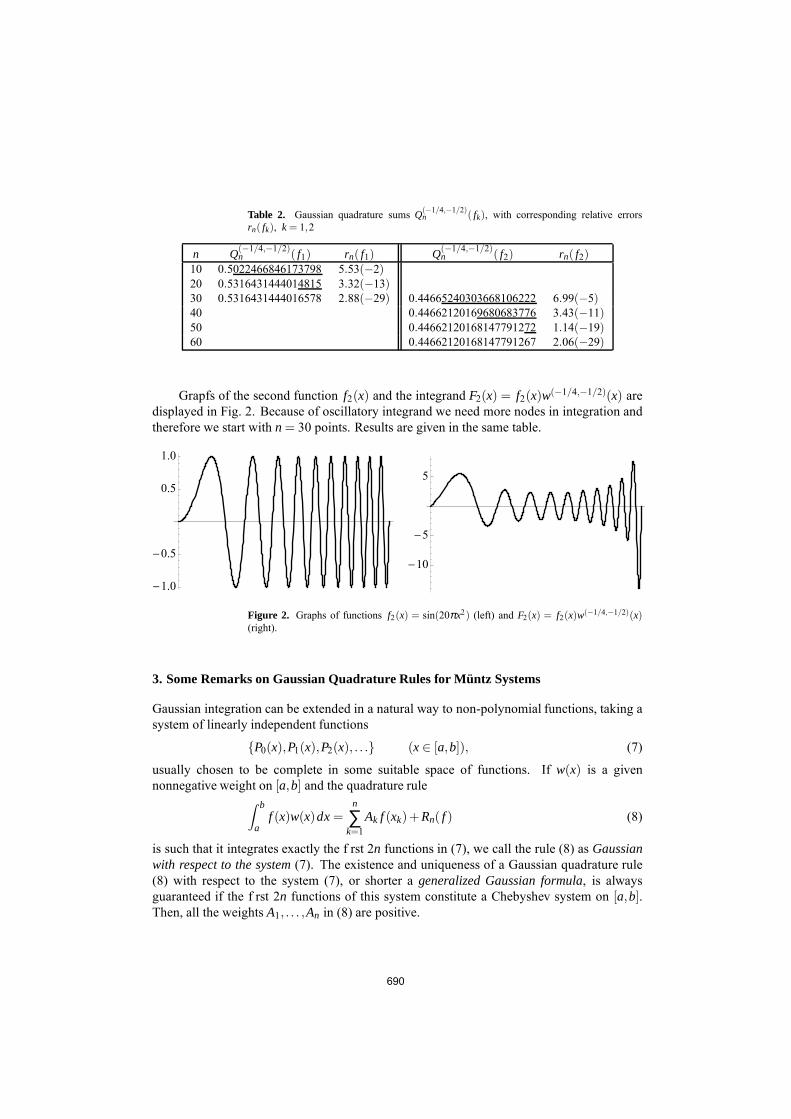
Table 2. Gaussian quadrature sums Q(−1/4,−1/2)n ( fk), with corresponding relative errors
rn( fk), k = 1,2
n Q(−1/4,−1/2)n ( f1) rn( f1) Q(−1/4,−1/2)
n ( f2) rn( f2)10 0.5022466846173798 5.53(−2)20 0.5316431444014815 3.32(−13)30 0.5316431444016578 2.88(−29) 0.44665240303668106222 6.99(−5)40 0.44662120169680683776 3.43(−11)50 0.44662120168147791272 1.14(−19)60 0.44662120168147791267 2.06(−29)
Grapfs of the second function f2(x) and the integrand F2(x) = f2(x)w(−1/4,−1/2)(x) aredisplayed in Fig. 2. Because of oscillatory integrand we need more nodes in integration andtherefore we start with n = 30 points. Results are given in the same table.
-1.0
-0.5
0.5
1.0
-10
-5
5
Figure 2. Graphs of functions f2(x) = sin(20πx2) (left) and F2(x) = f2(x)w(−1/4,−1/2)(x)(right).
3. Some Remarks on Gaussian Quadrature Rules for Müntz Systems
Gaussian integration can be extended in a natural way to non-polynomial functions, taking asystem of linearly independent functions
{P0(x),P1(x),P2(x), . . .} (x∈ [a,b]), (7)
usually chosen to be complete in some suitable space of functions. If w(x) is a givennonnegative weight on [a,b] and the quadrature rule
∫ b
af (x)w(x)dx=
n
∑k=1
Ak f (xk)+Rn( f ) (8)
is such that it integrates exactly the f rst 2n functions in (7), we call the rule (8) as Gaussianwith respect to the system(7). The existence and uniqueness of a Gaussian quadrature rule(8) with respect to the system (7), or shorter a generalized Gaussian formula, is alwaysguaranteed if the f rst 2n functions of this system constitute a Chebyshev system on [a,b].Then, all the weights A1, . . . ,An in (8) are positive.
690
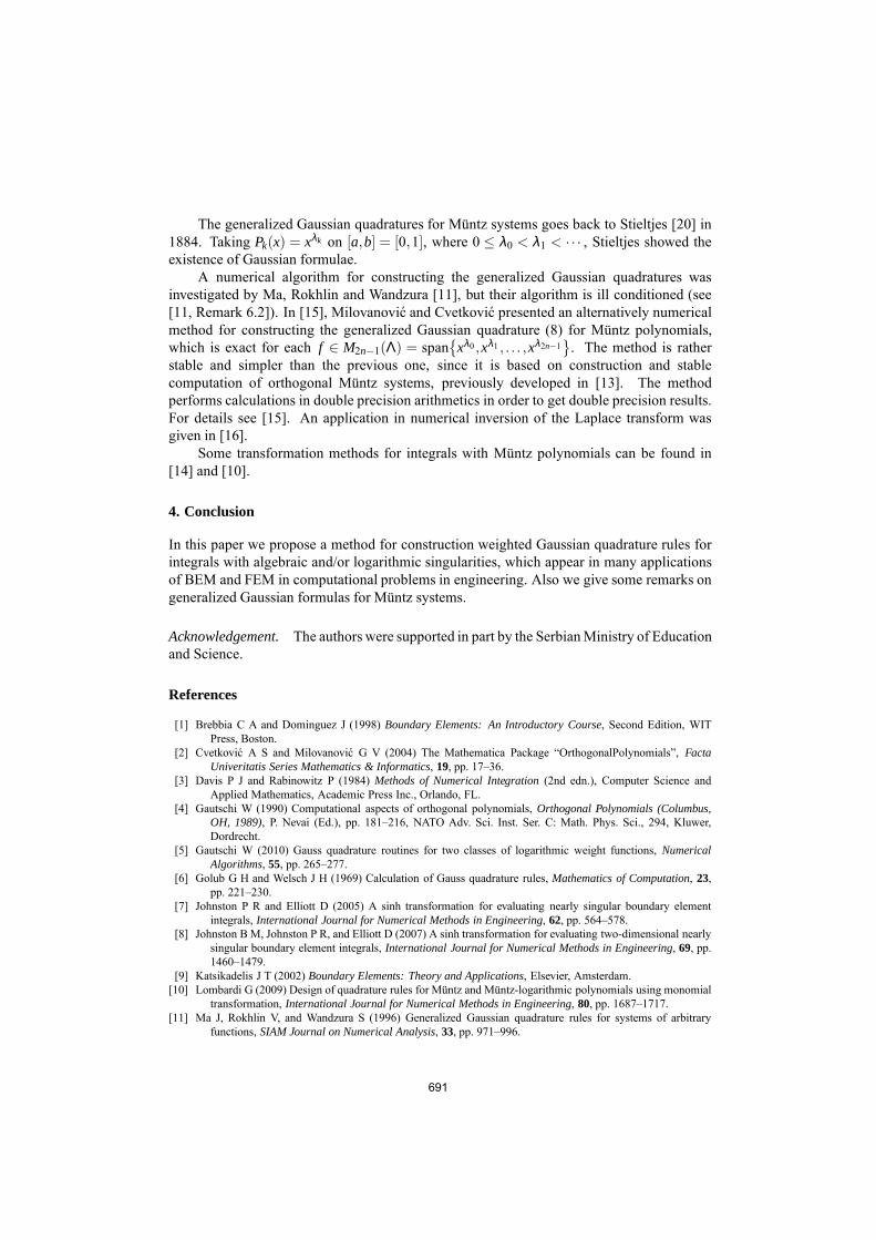
The generalized Gaussian quadratures for Müntz systems goes back to Stieltjes [20] in1884. Taking Pk(x) = xλk on [a,b] = [0,1], where 0 ≤ λ0 < λ1 < · · · , Stieltjes showed theexistence of Gaussian formulae.
A numerical algorithm for constructing the generalized Gaussian quadratures wasinvestigated by Ma, Rokhlin and Wandzura [11], but their algorithm is ill conditioned (see[11, Remark 6.2]). In [15], Milovanovic and Cvetkovic presented an alternatively numericalmethod for constructing the generalized Gaussian quadrature (8) for Müntz polynomials,which is exact for each f ∈ M2n−1(Λ) = span
{
xλ0 ,xλ1 , . . . ,xλ2n−1}
. The method is ratherstable and simpler than the previous one, since it is based on construction and stablecomputation of orthogonal Müntz systems, previously developed in [13]. The methodperforms calculations in double precision arithmetics in order to get double precision results.For details see [15]. An application in numerical inversion of the Laplace transform wasgiven in [16].
Some transformation methods for integrals with Müntz polynomials can be found in[14] and [10].
4. Conclusion
In this paper we propose a method for construction weighted Gaussian quadrature rules forintegrals with algebraic and/or logarithmic singularities, which appear in many applicationsof BEM and FEM in computational problems in engineering. Also we give some remarks ongeneralized Gaussian formulas for Müntz systems.
Acknowledgement.The authors were supported in part by the Serbian Ministry of Educationand Science.
References
[1] Brebbia C A and Dominguez J (1998) Boundary Elements: An Introductory Course, Second Edition, WITPress, Boston.
[2] Cvetkovic A S and Milovanovic G V (2004) The Mathematica Package “OrthogonalPolynomials”, FactaUniveritatis Series Mathematics & Informatics, 19, pp. 17–36.
[3] Davis P J and Rabinowitz P (1984) Methods of Numerical Integration(2nd edn.), Computer Science andApplied Mathematics, Academic Press Inc., Orlando, FL.
[4] Gautschi W (1990) Computational aspects of orthogonal polynomials, Orthogonal Polynomials (Columbus,OH, 1989), P. Nevai (Ed.), pp. 181–216, NATO Adv. Sci. Inst. Ser. C: Math. Phys. Sci., 294, Kluwer,Dordrecht.
[5] Gautschi W (2010) Gauss quadrature routines for two classes of logarithmic weight functions, NumericalAlgorithms, 55, pp. 265–277.
[6] Golub G H and Welsch J H (1969) Calculation of Gauss quadrature rules, Mathematics of Computation, 23,pp. 221–230.
[7] Johnston P R and Elliott D (2005) A sinh transformation for evaluating nearly singular boundary elementintegrals, International Journal for Numerical Methods in Engineering, 62, pp. 564–578.
[8] Johnston B M, Johnston P R, and Elliott D (2007) A sinh transformation for evaluating two-dimensional nearlysingular boundary element integrals, International Journal for Numerical Methods in Engineering, 69, pp.1460–1479.
[9] Katsikadelis J T (2002) Boundary Elements: Theory and Applications, Elsevier, Amsterdam.[10] Lombardi G (2009) Design of quadrature rules for Müntz and Müntz-logarithmic polynomials using monomial
transformation, International Journal for Numerical Methods in Engineering, 80, pp. 1687–1717.[11] Ma J, Rokhlin V, and Wandzura S (1996) Generalized Gaussian quadrature rules for systems of arbitrary
functions, SIAM Journal on Numerical Analysis, 33, pp. 971–996.
691

[12] Mastroianni G and Milovanovic G V (2008) Interpolation Processes – Basic Theory and Applications, SpringerMonographs in Mathematics, Springer – Verlag, Berlin – Heidelberg.
[13] Milovanovic G V (1999) Müntz orthogonal polynomials and their numerical evaluation, Applications andComputation of Orthogonal Polynomials, W Gautschi, G H Golub, and G Opfer (Eds.), pp. 179–202, ISNM,Vol. 131, Birkhäuser, Basel.
[14] Milovanovic G V and Cvetkovic A S (2002) Numerical integration of functions with logarithmic end pointsingularity, Facta Univeritatis Series Mathematics & Informatics, 17, pp. 57–74.
[15] Milovanovic G V and Cvetkovic A S (2005) Gaussian type quadrature rules for Müntz systems, SIAM Journalon Scientific Computing27, pp. 893–913.
[16] Milovanovic G V and Cvetkovic A S (2005) Numerical inversion of the Laplace transform, Facta UniveritatisSeries Electronics & Energetics, 18, pp. 515–530.
[17] Milovanovic G V and Velickovic D M (2001) Quadrature processes for several types of quasi-singular integralsappearing in the electromagnetic f eld problems, 5th Intern. Conf. Applied Electromagnetics PES 2001,Proceedings of Full Papers (Niš, 2001), D M Velickovic, (Ed.), pp. 117–122, Faculty of ElectronicEngineering, Niš.
[18] Oliveira S P, Madureira A L, and Valentin F (2009) Weighted quadrature rules for f nite element methods,Journal of Computational and Applied Mathematics,227, pp. 93–101.
[19] Piessens R and Branders M (1975) Tables of Gaussian Quadrature Formulas, University of Leuven, Leuven.[20] Stieltjes T J (1884) Sur une généralisation de la théorie des quadratures mécaniques, Comptes Rendus
Mathématique, Académie des Sciences, Paris, 99, pp. 850–851.
692
Third Serbian (28th Yu) Congress on Theoretical and Applied Mechanics Vlasina lake, Serbia, 5-8 July 2011 C-41
CRITERIA OF ELASTIC STABILITY FOR PLATE WITH GEOMETRIC DISCONTINUITY
Snežana N. Mitić Faculty of Mechanical Engineering, The University of Niš, Aleksandra Medvedeva 14, 18000 Niš e-mail: [email protected]
Abstract. This paper presents stability criteria for rectangular plates subjected to loads along constructive discontinuity and along the two edges. In its mid-plane, the plate is loaded with uniformly distributed forces along two opposing plate edges and along constructive discontinuity. The constructive discontinuity divides the plate into subplates of different thickness. The subplates are isotropic and have a common elastic surface area. The Morris-Levy method has been used to solve the stability problem. Each subplate buckling problem is separately solved and the solutions are brought together by matching the continuity equations. The plate has two opposite edges simply supported while the other two edges can take any combination of free, simply supported and clamped conditions. For different boundary conditions, the buckling solutions comprise of different combinations. For each boundary condition, the correct solution combination depends on the discontinuity load to the edges load ratio. The analysis of stability has been performed according to the basic postulates of the elastic stability theory. Fourth-order type ordinary linear differential equations with constant coefficients are derived from partial differential equations of the elastic surface areas of the buckled subplates. The buckling factor, which depends on the plate geometry, its mechanical properties and loads, is obtained from the derived system of equations.
1. Introduction The elastic buckling problem of rectangular plates under uniaxial loads acting at opposite edges is the most basic plate buckling problem and its solution is documented in all standard texts on plate buckling [1]. A theoretical analysis of the stability of plates with fields of non-uniform thickness is employed in practical engineering designs. Researchers have investigated various forms of thickness variations of the plate that include: a linear function along one direction [2]; a non-linear function along one direction [3] or in both directions [4]. Piecewise constant step functions in one direction are considered in references [5, 6], and in both directions in references [7]. The paper [8] considered stability criteria for rectangular plates subjected to intermediate and end in-plane loads. The subplates are of uniform thickness. Unlike [8], this paper will focus on subplates with different thickness. Subplates are isotropic and have a common elastic surface area. The resultant buckling problem can then be solved in the exact manner to yield the stability criteria that are functions of the position of the discontinuity and the relative ratio of the loads along discontinuity and edges. The Morris-Levy method has been used to solve the stability problem. Plates with constructive discontinuity and fields of non-uniform thickness are extensively used in modern structures. By using such plates, it is possible to obtain material saving,
693
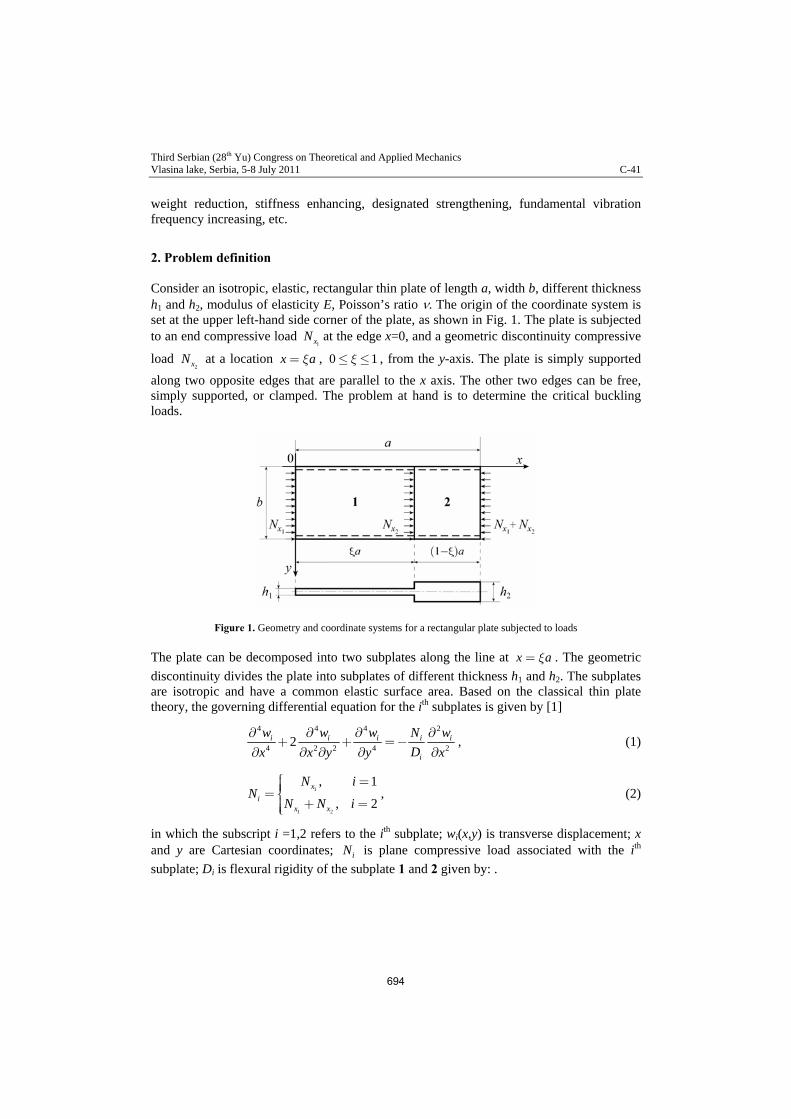
Third Serbian (28th Yu) Congress on Theoretical and Applied Mechanics Vlasina lake, Serbia, 5-8 July 2011 C-41
weight reduction, stiffness enhancing, designated strengthening, fundamental vibration frequency increasing, etc.
2. Problem definition Consider an isotropic, elastic, rectangular thin plate of length a, width b, different thickness h1 and h2, modulus of elasticity E, Poisson’s ratio . The origin of the coordinate system is set at the upper left-hand side corner of the plate, as shown in Fig. 1. The plate is subjected to an end compressive load
1xN at the edge x=0, and a geometric discontinuity compressive
load 2xN at a location x ax= , , from the y-axis. The plate is simply supported
along two opposite edges that are parallel to the x axis. The other two edges can be free, simply supported, or clamped. The problem at hand is to determine the critical buckling loads.
0 x£ £1
Figure 1. Geometry and coordinate systems for a rectangular plate subjected to loads
The plate can be decomposed into two subplates along the line at x ax= . The geometric
discontinuity divides the plate into subplates of different thickness h1 and h2. The subplates are isotropic and have a common elastic surface area. Based on the classical thin plate theory, the governing differential equation for the ith subplates is given by [1]
4 4 4
4 2 2 42i i i i
i
w w w N
D
2
2iw
x x y y x
¶ ¶ ¶ ¶+ + =-
¶ ¶ ¶ ¶ ¶, (1)
, (2) 1
1 2
, 1
, 2
x
ix x
N iN
N N i
ì =ïïï=íï + =ïïî
in which the subscript i =1,2 refers to the ith subplate; wi(x,y) is transverse displacement; x and y are Cartesian coordinates; is plane compressive load associated with the ith
subplate; Di is flexural rigidity of the subplate 1 and 2 given by: . iN
694

Third Serbian (28th Yu) Congress on Theoretical and Applied Mechanics Vlasina lake, Serbia, 5-8 July 2011 C-41
( )
31
1 212 1
EhD
n=
-, (3)
( )
32
2 212 1
EhD
n=
-. (4)
a) b)
Figure 2. . Geometry and coordinate systems for a rectangular plate subjected to loads.
(a) subplate 1; and (b) subplate 2.
3. Analytical modeling for subplate 1 Based on the classical thin plate theory, the governing differential equation for the subplate 1 is given by Eq. (1) for i=1 and can be rewritten as
1
4 4 41 1 1
4 2 2 411 1 1 1
2xNw w w
D
21
21
w
x x y y x
¶ ¶ ¶ ¶+ + =-¶ ¶ ¶ ¶ ¶
. (5)
Using the following transformations:
1 1 11 1 1, , ,
w x y aw x y
b a bq
x= = =
b= , (6)
the differential Eq. (5) of the deflection surface can be written in the following form:
4 4 4 2
2 2 4 4 2 2 21 1 114 2 2 4 2
1 1 1 1 1
2 0w w w w
Kx x y y x
x q x q p x q¶ ¶ ¶ ¶+ + +¶ ¶ ¶ ¶ ¶
1 = , (7)
where K1 is the buckling factor for subplate and which, for certain materials and load, depends on the dimensions of the plate.
1
2
1 21
xN bK
D p= . (8)
By using the Levy approach, solution of differential equations for the subplate 1 can be expressed as:
695

Third Serbian (28th Yu) Congress on Theoretical and Applied Mechanics Vlasina lake, Serbia, 5-8 July 2011 C-41
( ) ( )1 1 1 1 1 1, sin ,n nw x y f x y nb b= p= (9)
where n (=1, 2, ...) is the number of half waves of the buckling mode in the y direction and ( )1 1f x is an unknown function to be determined. Eq. (9) satisfies the boundary conditions
for two simply supported edges. The essential and natural boundary conditions for the two simply supported edges at
1 0y = and 1 1,y = associated with the subplate 1 are given by
( )1
1 1 1 0,1,
yw x y
== 0 (10)
( ) ( )
1
2 21 1 1 1 1 1
2 2 2 21 1 0,1
, ,0
y
w x y w x y
y x
nx q
=
é ù¶ ¶ê +ê ¶ ¶ê úë ûú =ú (11)
The transverse displacement given in Eq. (9) satisfies the boundary conditions of the two parallel simply supported edges [Eq. (10) and (11)]. In view of Eq. (9), the partial differential equations may be reduced to fourth-order ordinary differential equations as
( ) ( ) ( ) ( ) ( )4 2 2 2 4 4 4 2 2 21 1 1 1 1 1 1 1 12 0n nf x f x f x K f xx q b x q b p x q¢¢ ¢¢- + + .= (12)
The buckling of subplate 1 in the direction of the x axis is determined by the functions
( )1 1f x which is represented in the form
1111
xeAxf (13)
Based on Eq. (13), Eq. (12), the characteristics equation for subplate 1 is derived
(14) ( )4 2 2 2 2 2 2 2 4 4 41 2 n nKl p x q x q b l x q b+ - + 0.=
q
0.
Introduce a label , equation (14) becomes: 2 2 21 1Kg p x=
(15) ( )4 2 2 2 2 4 4 41 2 n nl g x q b l x q b+ - + =
Depending on the roots of the characteristics equations of the differential equations, there are five general solutions to the above fourth-order differential equations as given below.
3.1. Solution A for the case 1<0 The general solution of the differential equation (7) has the form
( )1 1 1 1 2 1 1 3 1 1 4 1 1 1sinh cosh sinh cosh sin nw C x C x C x C x ya a b b= + + + b . (16)
where and are the roots of the characteristics equation (15) for condition 1<0: 1a 1b
( )2 2 2 2 2 2 21 11,2 1 1 1 12 22 4n nl g x q b g x q b g a= - - - - = , (17)
696

Third Serbian (28th Yu) Congress on Theoretical and Applied Mechanics Vlasina lake, Serbia, 5-8 July 2011 C-41
( )2 2 2 2 2 2 21 13,4 1 1 1 12 22 4n nl g x q b g x q b g= - - + - =b . (18)
3.2. Solution B for the case 1=0 For the roots of the characteristics Eq. (15) are: 1 0g =
. (19) 1 1 na b xqb= =
General solution of the differential equation for those roots of characteristics equations is:
( )1 1 1 1 2 1 1 1 3 1 1 4 1 1 1 1sinh sinh cosh cosh sin nw C x C x x C x C x x ya a a a= + + + b . (20)
3.3. Solution C for the case 2 2 210 4 ng x q b< <
The roots of the characteristics equation (15) are
12 2 2 11,2 4 2n i
ggl x q b= - + , (21)
12 2 2 13,4 4 2n i
ggl x q b= - - , (22)
where
12 2 2 11 1;
4 2n
gga x q b b= - = (23)
The general solution of the differential equation (7) has the form:
(
)1 1 1 1 1 1 2 1 1 1 1
3 1 1 1 1 4 1 1 1 1
sinh cos cosh cos
sinh sin cosh sin sin n
w C x x C x x
C x x C x x
a b a b
a b a b b
= +
+ + 1y
+. (24)
3.4. Solution D for the case 2 2 21 4 ng x q b=
The roots of the characteristics equation (15), for this case are:
(25) 1 1 na b xqb= =
The general solution of the differential equation (7) has the form
( )1 1 1 1 2 1 1 1 3 1 1 4 1 1 1 1cos cos sin sin sin nw C x C x x C x C x x ya a a a= + + + b . (26)
697

Third Serbian (28th Yu) Congress on Theoretical and Applied Mechanics Vlasina lake, Serbia, 5-8 July 2011 C-41
3.5. Solution E for the case 2 2 2
1 4 ng x q b>
The roots of the characteristics equation (15), for this case are:
( )2 2 2 2 2 2 21 11,2 1 1 1 12 22 4n ni il g x q b g x q b g a= - - - = , (27)
( )2 2 2 2 2 2 21 13,4 1 1 1 12 22 4n ni il g x q b g x q b g= - + - = b . (28)
The general solution of the differential equation (7) is
( )1 1 1 1 2 1 1 3 1 1 4 1 1 1cos sin cos sin sin nw C x C x C x C x ya a b b= + + + b . (29)
The constants C1, C2, C3 and C4 in Eq. (16), (20), (24), (26) and (29) are determined from the boundary conditions along the edges and the continuity conditions along the geometric discontinuity.
4. Analytical modeling for subplate 2 Based on the classical thin plate theory, the governing differential equation for subplate 2 is given by [1]:
1 2
4 4 42 2 2
4 2 2 422 2 2 2
2x xN Nw w w
D
22
22
w
x x y y x
+¶ ¶ ¶ ¶+ + =-¶ ¶ ¶ ¶ ¶
, (30)
where is the transverse displacement for subplate 2. 2 2 2,w x y Using the following transformations:
( )
2 2 22 2 2, , ,
1
w x y aw x y
b a bq
x= = =
- b= , (31)
the differential Eq. (30) of the deflection surface can be written in the following form:
( ) ( ) ( )( )4 4 4
2 4 22 4 2 22 2 214 2 2 4
2 2 2 2
2 1 1 1 1 0w w w
Kx x y y
x q x q p e x q¶ ¶ ¶+ - + - + Y + - =¶ ¶ ¶ ¶ ¶
22
22
w
x
¶ , (32)
where K2 is the buckling factor for subplate 2:
( )
1 2
2
2 22
x xN N bK
D p
+= , (33)
and
3
1 1
2 2
D h
D h
æ ö÷ç ÷Y = =ç ÷ç ÷çè ø; 2
1
x
x
N
Ne= . (34)
698

Third Serbian (28th Yu) Congress on Theoretical and Applied Mechanics Vlasina lake, Serbia, 5-8 July 2011 C-41
By using the Levy approach, solution for differential equation for the subplate 2 can be expressed as:
( ) ( )2 2 2 2 2 2, sin ,n nw x y f x y nb b= p= . (35)
where n (=1, 2, ...) is the number of half waves of the buckling mode in the y direction and
( )2 2f x is an unknown function to be determined. Eq. (35) satisfies the boundary conditions
for two simply supported edges. The essential and natural boundary conditions for the two simply supported edges at
1 0y = and 1 1,y = associated with the subplate 2 are given by
( )2
2 2 2 0,1,
yw x y
== 0 , (36)
( )
( )( )
2
2 22 2 2 2 2 2
2 2 222 2
0,1
, ,0
1y
w x y w x y
y x
nx q
=
é ù¶ ¶ê +ê ¶ ¶ê ú-ë û
ú =ú . (37)
The transverse displacement given in Eq. (35) satisfies the boundary conditions of the two parallel simply supported edges [Eq. (36) and (37)]. In view of Eq. (35), the partial differential equations in Eq. (32) may be reduced to fourth-order ordinary differential equations as
( ) ( ) ( ) ( ) ( ) ( ) ( ) ( )2 44 2 2 4 4 2 2 22 2 2 2 2 2 1 2 22 1 1 1 0.n nf x f x f x K f xx q b x q b p k x q¢¢ ¢¢- - + - + Y + = (38)
The buckling of subplate 2 in the direction of the x axis is determined by the functions 22 xf which is represented in the form
2'
222xeAxf (39)
The characteristics equation for subplate 2 is derived
( ) (40) ( )( ) ( ) ( ) ( )4 22 2 42 2 2 2 4 41 1 1 2 1 1nKl p x q x q b l x q bé ù¢ ¢+ Y +Y - - - + - =ê úë û
0.n
21
Introduce a label
( )( )222 1 1 Kg p e x q= Y + - (41)
equation (40) becomes
(42) ( ) ( ) ( ) ( )4 22 42 2 4 42 2 1 1 0.nl g x q b l x q bé ù¢ ¢+ - - + - =ê úë û n
Depending on the roots of the characteristics equations of the differential equations, there are five general solutions to the above fourth-order differential equations as given below.
699

Third Serbian (28th Yu) Congress on Theoretical and Applied Mechanics Vlasina lake, Serbia, 5-8 July 2011 C-41
4.1. Solution A for the case <0 The general solution of the differential equation (32) has the form
( )2 5 2 2 6 2 2 7 2 2 8 2 2sinh cosh sinh cosh sin nw C x C x C x C x ya a b b= + + + 2b (43)
where and are the roots of the characteristics equation (42) for the condition 1<0: 1a 1b
( )( ) ( )2 22 2 2 2 21 11,2 2 2 2 22 22 1 4 1n nl g x q b g x q b g a¢ = - - - - - - = , (44)
( )( ) ( )2 22 2 2 2 21 13,4 2 2 2 22 22 1 4 1nl g x q b g x q b g b¢ = - - - + - - =n . (45)
4.2. Solution B for the case 2=0 For the roots of the characteristics Eq. (42) are: 2 0g =
1 1 1 n . (46)
The general solution of the differential equation (32) is
( )2 5 2 2 6 2 2 2 7 2 2 8 2 2 2 2sinh sinh cosh cos sin nw C x C x x C x C x x ya a a a= + + + b
b
. (47)
4.3. Solution C for the case ( )2 2 220 4 1 ng x q< < -
The roots of the characteristics Eq. (42) are:
2 22 2 21,2 1
4 2n i
, (48)
2 22 2 23,4 1
4 2n i
, (49)
where
2 22 22 1 ;
4 2n 2
. (50)
The general solution of the differential equation (32) for subplate 2 has the form
(
)2 5 2 2 2 2 6 2 2 2 2
7 2 2 2 2 8 2 2 2 2 2
sinh cos cosh cos
sinh sin cosh sin sin n
w C x x C x x
C x x C x x
a b a b
a b a b b
= +
+ + y
+. (51)
700

Third Serbian (28th Yu) Congress on Theoretical and Applied Mechanics Vlasina lake, Serbia, 5-8 July 2011 C-41
b4.4. Solution D for the case ( )2 2 2
2 4 1 ng x q= - The general solution of the differential equation (32) for subplate 2 is:
2 5 2 2 6 2 2 2 7 2 2 8 2 2 2 2cos cos sin sin sin nw C x C x x C x C x x y
b
, (52)
where
. (53) ( )2 2 1 nb a x qb= = -
4.5. Solution E for the case ( )2 2 22 4 1 ng x q> -
The roots of the characteristics Eq. (42) are:
2 2' 2 2 2 21,2 2 2 2 2
1 12 1 4 1
2 2ni i2n (54)
2 2' 2 2 2 23,4 2 2 2 2
1 12 1 4 1
2 2ni i2n (55)
The general solution of the differential equation (32) has the form:
2 5 2 2 6 2 2 7 2 2 8 2 2cos sin cos sinw C x C x C x C x . (56)
The constants C5, C6, C7 and C8 in Eq. (43), (47), (51), (52) and (56) are determined from the boundary conditions along the edges and the continuity conditions along the geometric discontinuity. The essential and natural boundary conditions of the plate at the edge 1 0x = for simply
supported edge are defined as follows:
1
1
2 21 1
1 0 2 2 2 21 1 0
10, 0x
x
w ww
x yn
x q==
é ù¶ ¶ê= +ê ¶ ¶ë ûú =ú . (57)
For a clamped edge natural boundary conditions are defined as follows:
1
11 0
1
0, 0x
ww
x=¶=¶= . (58)
For a free edge boundary conditions are defined:
1 1
2 2 3 31 1 1 1 1 1
2 2 2 2 3 3 3 2 3 311 1 1 1 10 0
1 1 20, 0
x x
w w w w w
xx y x x y
gnnxqx q x q x q
= =
é ù é¶ ¶ ¶ ¶ ¶-ê ú ê+ = + +ê ú ê ¶¶ ¶ ¶ ¶ ¶ë û ë
ùú =úû
. (59)
The essential and natural boundary conditions of the plate at the edge 1 0x = for simply
supported edge are defined as follows:
701

Third Serbian (28th Yu) Congress on Theoretical and Applied Mechanics Vlasina lake, Serbia, 5-8 July 2011 C-41
2
2
2 22 2
2 1 2 2 222 2
1
10, 0
1x
x
w ww
x y
. (60)
For a clamped edge natural boundary conditions are defined as follows:
2
2
22 1
2 1
0, 0x
x
ww
x==
é ù¶ê ú= ê ú¶ë û= . (61)
For a free edge boundary conditions are defined:
( )
( ) ( ) ( )
2
2
2 22 2
2 2 222 2
1
3 32 2 2 2
3 3 2 2 33 2 32 2 2 2
1
10,
1
1 20
1 1 1
x
x
w w
x y
w w w
x x y x
nx q
gnx q x q x q
=
=
é ù¶ ¶ê ú+ =ê ú¶ ¶ê ú-ë ûé ù¶ ¶ ¶-ê ú+ +ê ú¶ ¶ ¶ ¶ê ú- - -ë û
=
(62)
To ensure displacement continuities and equilibrium conditions at the interface of the two subplates, the following essential and natural conditions must be satisfied:
1 2
1 21xw w
==
0x = (63)
( )
1 2
1
1 21 0
1 1
1x x
w
x xxq x q= =
¶ =¶ - ¶
2w¶ (64)
( )
12
2 2 2 21 1 2 2
1 1 2 22 2 2 2 2 2 221 1 2 21 0
1 1
1x x
w w w wD D
x y x yn n
x q x q= =
é ùé ù¶ ¶ ¶ ¶ê úê ú+ = +ê úê ú¶ ¶ ¶ ¶ê ú-ë û ë û (65)
( ) ( ) ( )
1
2
3 31 1 1 1
1 3 3 3 2 3 311 1 1 1
3 32 2 2 2 2
2 3 3 2 33 322 2 2
0
1 2
21
11 1
x
x
w w wD
xx x y
w wD
xx x y
gnxqx q x q
n gx qx q x q
=
=
é ù¶ ¶ ¶-ê ú+ + =ê ú¶¶ ¶ ¶ë ûé ù¶ - ¶ ¶ê ú+ +ê ú- ¶¶ ¶ ¶ê ú- -ë û
w (66)
When assembling the subplates to form the whole plate via the implementation of the boundary conditions of the plate along the two edges parallel to the y-axis [Eq. (57)–(62)] and the interface conditions between two subplates [Eq. (63)–(66)], a system of homogenous equations is obtained. For a nontrivial solution, the determinant of system must vanish. Each solution combination for the determinant of system is examined. The valid solution combinations should satisfy the following requirements: the buckling loads satisfy the limits of validity for the solution combinations which they belong to; the buckling load factor is the lowest value among possible solutions; the stability curves are continuous.
702

Third Serbian (28th Yu) Congress on Theoretical and Applied Mechanics Vlasina lake, Serbia, 5-8 July 2011 C-41
5. Numerical results Exact stability criteria are presented graphically in Figs. 3 to 6 for simply supported (SS), and free (FF) plates, respectively.
5.1. SSSS plate A simply supported rectangular plate (or simply referred to as an SSSS plate) subjected to geometric discontinuity and end inplane loads is first considered. Fig. 3 presents the typical stability criterion curves for SSSS plates. Fig. 3. shows the buckling factor K1 in the function of the position of the geometric discontinuity for different loads ratio (
2xN =const) and h2/h1=1.5, =1.
With the increase of coordinate , the value of K1 decreases. For constant position of the geometric discontinuity, the value of K1 decreases with the increase of loads ratio (
2xN =const, 1x
N decreases).
0.2 0.3 0.4 0.5 0.6 0.7 0.8 0.9 1.0
4
6
8
10
e = 0
e = 0.2
e = 0.5
e = 0.7
e = 1.2
e = 1.6
K1
x
q = 1h2 / h
1 =1.5
4.00
Figure 3. The buckling factor K1 in the function of the position
of the geometric discontinuity for different loads ratio for SSSS plate
In Fig. 4. the buckling factor K2 in the function of loads ratio (2xN =const) for different
position of the geometric discontinuity and h2/h1=1 is represented. The factor K2 increases with the increase of loads ratio . With the moving of the position of the discontinuity toward higher values, the value of the buckling factor K2 increases for constant loads ratio . The stability region is bellow the boundary curves.
703

Third Serbian (28th Yu) Congress on Theoretical and Applied Mechanics Vlasina lake, Serbia, 5-8 July 2011 C-41
0.0 0.2 0.4 0.6 0.8 1 0
3.0
3.5
4.0
4.5
5.0
5.5
6.0
6.5
.
x =0.3 x =0.5 x =0.7 x =0.9
K2
e
h2 / h
1 =1
q = 1
Figure 4. The buckling factor K2 in the function of loads ratio the for different position of the geometric discontinuity for SSSS plate
5.2. FSFS plate
Rectangular plate with the two edges parallel to the x-axis simply supported while the two edges parallel to the y-axis are free (this plate is referred to as a FSFS plate) is consider. The typical stability criterion curve for a FSFS plate. is shown in Fig. 5. Also, Fig. 5. depicts the buckling factor K1 in the function of the position of the geometric discontinuity for different loads ratio . The geometric properties plates are h2/h1=1.2 and =1. With the moving of the position of the discontinuity toward higher values, the value of the buckling factor K1 decreases.
0.0 0.1 0.2 0.3 0.4 0.5 0.6 0.7 0.8 0.9 1.0
1.5
2.0
2.5
3.0
3.5
4.0
q = 1h2 / h
1 =1.2
e = 0
e = 0.2
e = 0.5
2.049
e = 0.7
K1
x Figure 5. The buckling factor K1 in the function of the position
of the geometric discontinuity for different loads ratio for FSFS plate
704

Third Serbian (28th Yu) Congress on Theoretical and Applied Mechanics Vlasina lake, Serbia, 5-8 July 2011 C-41
The buckling factor K2 in the function of loads ratio the for different position of the geometric discontinuity is presented in Fig. 6. Stability region is bellow boundary curves. The value of the buckling factor K2 increases with the moving of the position of the discontinuity toward higher values.
0.0 0.1 0.2 0.3 0.4 0.5 0.6 0.7 0.8 0.9
1.6
1.8
2.0
2.2
2.4
2.6
2.8
q = 1h2 / h
1 =1.2
e = 0.7
e = 1.2
e = 1.6
K2
x
2.049
Figure 6. The buckling factor K2 in the function of loads ratio the for different position of the geometric discontinuity for FSFS plate
6. Conclusion This paper is concerned with the elastic buckling of rectangular plates subjected to both geometric discontinuity and end uniaxial loads. The stability of a rectangular plate with geometric discontinuities has been discussed in the field of elastic stability. The rectangular plates have two simply supported opposite edges, while the other two plate edges can have free, simply supported, or clamped edges. The aforementioned buckling problem is solved by decomposing the plate into two subplates at the location where the geometric discontinuity uniaxial load acts. By applying the Levy method of the boundary conditions and the conditions along the geometric discontinuity, a system of equations has been derived. Based on the obtained solution, numerical analysis has been performed. Stability criteria (the buckling factor) in the function of plate thickness ratio, loads ratio and the position of the geometric discontinuity are obtained. The method gives exact stability criteria; samples of which are presented in a graphical form for plates with various boundary conditions. Some sample buckling results are served as benchmark solutions for researchers who are developing software for plate buckling analysis.
705

Third Serbian (28th Yu) Congress on Theoretical and Applied Mechanics Vlasina lake, Serbia, 5-8 July 2011 C-41
References [1] Timoshenko P.S. and James G. M. (1961) Theory of Elastic Stability, McGraw-Hill, Book Company, Inc. [2] Wittrick W. H. and Ellen C. H. (1962) Buckling of tapered rectangular plates in compression, Aeronautical
Quarterly 13, pp. 308-326.. [3] Malhorta S. K., Ganesan N. and Veluswami M. A. (1987) Vibrations of orthotropicsquare plates having
variable thickness (parabolic variation), Journal of Sound and vibration 119, pp. 184-188.. [4] Olhoff N. (1974) Optimal design of vibrating rectangular plates, International Journal of Solids and
Structures 10, pp. 93-109. [5] Guo S. J., Keane A. J. and Moshrefi-Torbati M. (1997) Vibration analysis of stepped thickness plates, Journal
of Sound and vibration 204, pp. 645-657. [6] Eisenberger M. and Alexandrov A. (2000) Stability analysis of stepped thickness plates, Computational
Methods for Shell and Spatial Structures, IASS-IACM 2000 Athens, Greece: ISASR-NTUA. [7] Ju F., Lee H. P. and Lee K. H. 1995 Free vibration of plates with stepped variations in thickness on non-
homogeneous elastic foundations.Journal of Sound and vibration 183, 533-545. [8] Wang C. M., Chen Y. and Xiang Y. (2004) Stability criteria for rectangular plates subjected to intermediate
and end inplane loads, Thin-Walled Structures 42, pp. 119–136
706
Third Serbian (28th Yu) Congress on Theoretical and Applied Mechanics Vlasina lake, Serbia, 5-8 July 2011 C-43
VIBRATIONS AND NOISE AS DESIGN CONSTRAINTS IN MACHINE SYSTEMS DESIGN
M. Ognjanovic, M. Benur Faculty of Mechanical Engineering, The University of Belgrade, Kraljice Marije 16, 11120 Belgrade 35 e-mail: [email protected]
Abstract. Vibrations of machine systems are important indicator of the system quality and of dynamic process which going on inside of the system. In reverse approach for design necessity, vibration indicators can be used as design limits (constraints) in order to choose and harmonized design parameters which can provide high level of technical system quality. As the case study, the robust design approach in the stage of the Embodiment design of power transmission components – gear systems is presented. For this purpose the specific model of gear vibrations is developed which is suitable for applying as the design constraint. The model is based on a great volume of experimental data about gear units vibrations and modal analysis, etc. Theoretical knowledge and models are insufficient yet to provide the necessary data. The article contains presentation of testing methods and data processing oriented to provide data necessary for the application in the suggested approach to power transmission components design. Additionally the article includes analysis of disturbance energy (power) absorption through the mechanical (elastic) structure, attenuation and emission in surroundings. The methodology of vibration and noise reduction is based on design parameters variation with objective to reduce disturbance energy and increase or kip at the same level of reliability and other service quality indicators. Keywords: vibrations, gears, robust design
1. Introduction
Design for Vibration and Noise is one of separate approaches Design for X – DfX which in the design stage of Embodiment design provides environment for optimal design parameters definition in the first attempt. Robust design is a specific approach aimed to design parameters definition which can provide design solution insensitive at functional requirements variation [1-3]. This design advantages are provided by design constraints which are result of DfX methodology as well as reliability as design constraint, vibration as design constraint, noise as design constraint, cost as design constraint etc. This research presents by itself completing and spreadsheet of design methodology by incorporating the knowledge from various areas of techniques. In order to incorporate vibration and use as design constraint, it is necessary to identify the process of vibration generation in the certain technical system and then use this mechanism in reverse direction as design constraint. As the case study for this opportunity is chosen design parameters definition of the gear drive units. The gear systems present very specific assembly of mechanical components in the sense of vibration and noise generation. This is combination of discrete and continual dynamic system and interaction of design parameters have significant effect at vibration and noise indicators.
707

Third Serbian (28th Yu) Congress on Theoretical and Applied Mechanics Vlasina lake, Serbia, 5-8 July 2011 C-43
2. Vibration and Noise as Design Constraints Vibration and noise of machine systems, i.e. power transmission components is the result of interaction between disturbances caused by components in motion and design parameters of components. This interaction in gear teeth meshes and bearings are in the form of machine parts collision, sliding, rolling etc [3-6]. In gear pair meshes between the meshed teeth all of these processes exist. A few kinds of teeth impacts arise in the mesh. More important is the addendum impact which is the result of gear pitch difference caused by elastic deformations. 2.1 Gear system restorable free vibrations
Teeth deformations are proportional to teeth load and teeth stiffness. Deformations replace the first point of contact from the right position A, to position A’ which is ahead of point A. The contact of teeth pair starts with intensive addendum impact (Fig.1a). Collision speed vc is proportional to teeth deformation, speed of rotation n and gear design parameters. By analyzing teeth geometry, deformations and speeds, collision speed at the first point of teeth contact is defined and presented in [7 and 8]. Every individual teeth impact produces natural free vibration of the gears (Fig 1b) with natural frequency fn . By strong inside damping these vibrations attenuate in a short time. The next teeth pair entering the mesh collides again and again. Vibrations become restorable after every teeth impact. For relatively slow gear rotation the measured time function of restorable free vibrations is presented in Fig. 2a. The teeth mesh frequency f corresponds to gear revolutions and to gear teeth number. If the speed of the gear rotation is slow enough, the time between the two teeth impacts 1/f is higher than the time necessary for the free vibration attenuation.
Figure 1. Gear teeth addendum collision (a) and free vibration caused by teeth impact (b)
As the speed of rotation increases the time between the two impacts gets lesser and lesser with the same natural frequency fn. In the full resonance these two frequencies get equal f=fn. For the case of gear vibration measurement (Fig 2b) (gear teeth number z=32) the resonant speed of gear rotation is 9860 rpm, and resonant teeth mesh frequency is 5258 Hz. Before the main resonance a few sub-resonances arise. This is the result of equality of additional disturbances and natural frequencies. After (behind) the main resonance arises, numerous super-critical resonances arise and total vibration level slightly increase. This is an interesting phenomenon, especially in the gear meshing process. In super-critical mesh
708

Third Serbian (28th Yu) Congress on Theoretical and Applied Mechanics Vlasina lake, Serbia, 5-8 July 2011 C-43
frequency range the absorbed disturbance energy by teeth impact relishes natural free vibrations. Higher speed of rotation produces higher level of absorbed disturbance energy and relished vibration energy has to be of higher level. Also, in super-critical mesh frequency range the modal structure of gear system fluctuates. In some parts of this range energy attenuation is lesser and relished energy by natural vibration is higher. By extensive measurement of gear vibrations with speed of rotation variation [7-8] and with frequency spectrum analysis these processes are identified.
Figure 2. Restorable free vibration of gear pair: a) the time function, b) result of vibration measurement and modeling
The results of those gear vibration measurement are presented in the form of calculation model [7-8]. The objective of modeling was to prove the hypothesis that gear vibration is a restorable natural one and then to present the vibrations in the form suitable for use as constraints in design parameters definition in gear drive design process. The total level of gear vibration is divided into two parts, continual and transient (Fig. 2b). x ax bx
sin1sin1 0T
eTaba f
m
xcAxxxx (1)
The gear pair is modeled as a single mass oscillator, where me is equivalent mass reduced in collision direction (Fig.1a), c is the mean gear teeth stiffness, x0 is teeth deformation amplitude in the moment of teeth collision, T is transfer function between force transferred
709

Third Serbian (28th Yu) Congress on Theoretical and Applied Mechanics Vlasina lake, Serbia, 5-8 July 2011 C-43
to the gear masses and collision force Fc with phase angle is coefficient of energy absorption inside the vibration system, and f is the gear teeth mesh frequency. The model presented by equation (1) and by the diagram in Fig.2b is developed using the theory of singular systems. According to this theory, the singular process consists of the two processes, continual and transient. Vibration energy emission is presented as the continual process (a) and transient (b) which contains resonances (the main, sub-critical and super-critical). Analytical model for continual part is established based on equilibrium between disturbance energy caused by teeth impacts and kinetic energy of restorable free vibrations. A significant part of disturbance energy is attenuated by numerous damping. The ratio between these energies is presented in the form of constant value which is calculated for measured vibrations level. The model for additional (transient) vibration values (b) is developed using analytical relations for resonance responses. These formulas include the difference between the teeth mesh (impact) frequency f and natural frequency fn, dimensionless damping coefficient and phase angle. By variation of damping coefficient the response is calculated to be equal measured vibrations. In Fig.2b the calculated line which approximates the measured one is presented. This line contains the main resonance only. The program for these values calculation can also include sub-critical and super-critical resonances. The developed analytical model gives possibility to present disturbance energy transformation, and to explain the inside processes of gear teeth mesh. Besides, the model gives possibility for design parameters harmonization in order to avoid resonances and reduce gear vibration level, i.e. use gear vibration as design constraints. 2.2 The noise generation caused by gear system vibration The part of disturbance energy absorbed by teeth repeatable collisions is relished in the form of kinetic energy of the gear system vibrations. The part of this kinetic energy is transformed, via free surfaces, into the noise energy inside the gear system housing. Another part of energy is transmitted through the supports (bearings) to the housing walls. This energy can be emitted from the wall surface in the surroundings in the form of noise waves. Also, the housing inside noise can penetrate through the housing walls into the surroundings. Much more important effect of the gear system vibration is disturbance of gear housing natural vibrations. This vibration can significantly intensify the noise that housing surfaces emit into the surroundings. From this point of view, the housing walls have a triple role: transmitter of vibration energy in surrounding, insulator of inside noise and generator of additional noise by own natural vibrations. Detailed analysis of the gear system housing behavior and its effects are presented in the articles [9-10]. Disturbing of a certain modal shape of elastic deformation with a certain natural frequency fni is the result of a few conditions, equality of natural and disturbing frequency, the same direction and type of elastic deformation of disturbance elastic waves and modal elastic deformations, low level of dimensionless damping coefficient of those modal elastic deformations (elastic waves). In Fig. 3a and b, numerical anaysis of natural frequencies by FEM, and by modal testing of chosen gearbox housing, is presented. Fig.3c shows response caused by modal hammer impact which contains the great collection of natural frequencies which are disturbed. Four of them fn1… fn4 have dominant effect. If inside the housing the running gear system with mesh (teeth impact) frequencies f1, f2 and f3 increase with speed of rotation, those frequencies proportionally increase. Equality of disturbance fi and natural fni frequencies produces natural vibrations of housing walls and noise with this frequency.
710

Third Serbian (28th Yu) Congress on Theoretical and Applied Mechanics Vlasina lake, Serbia, 5-8 July 2011 C-43
b) a)
Figure 3. Relation between frequencies of gear system vibration
d) c)
and gear housing natural frequencies
The relation between disturbance and natural frequencies presented in Fig. 3d is a principle one and presents Campell’s diagram for this purpose. A real gear system which is settled in the gearbox housing generates vibrations with a much more complex frequency spectrum. Except the presented teeth mesh frequencies f1, f2 and f3 (Fig.3d) natural frequencies of the gear system dominate in those spectrums. Furthermore, gear system vibrations disturb natural vibrations of housing walls. However, all natural vibrations are independent of service conditions (speed of rotation) and are in close relation with design parameters. This is the reason why some of the gear system natural frequencies can permanently disturb some of the housing natural frequencies and produce permanent high level of noise with a certain frequency. It can be changed by some kind of design parameters variation. 2.3 Disturbance power transmission Disturbance power transmits through the gear unit assembly and can be indicated by outside motion of discrete masses and by inside motion of elastic waves in machine parts [11]. Motion of discrete masses can indicate disturbance power transmission in the form of the next relations as follows.
fxK
W cc 2 ; f
xmfEW e
kv 2
2 ;
c
vv W
W ;
v
ss W
W (2)
The teeth collision power Wc is proportional to constant K proportional to teeth collision force (gear design parameters and collision speed) and fluctuation of teeth displacement xc
711

Third Serbian (28th Yu) Congress on Theoretical and Applied Mechanics Vlasina lake, Serbia, 5-8 July 2011 C-43
and teeth mesh frequency f. The gear vibration power Wv is proportional to the rotating equivalent mass me, the vibration speed (obtained via equat.1) and the teeth mesh frequency f. Disturbance power transfer function from collision power to vibration power is marked by v and transfer function from vibration power to the sound power is marked by s. All of them are experimental values which are in this way very simply presented.
x
The part of absorbed disturbance energy is transmitted through elastic structure of machine part in the form of elastic waves. By reflections from bound surfaces of machine part, the dominant value of that energy attenuates. In the course of attenuation process elastic waves reflect from bound surfaces. Via contact surfaces the part of wave energy is transmitted to the other machine part in the assembly. In Fig.4 the assemblies of the gear, shaft, bearing and support in housing wall are presented. The part of disturbance power absorbed in gear mesh Wg is transmitted to the shaft Wsh with the transmission factor gshshgT WW .
The part of disturbance energy via other gear bound surfaces is transmitted into inside space of transmission unit in the form of inside sound power Win with the transmission factor gininT WW . The rest of disturbance power Wg attenuates inside of the gear
elastic structure i.e. attenuated power is Wga=Wg-Wsh-Win . Disturbance power transmitted to the shaft Wsh is partly transmitted via the bearings to the transmission unit housing Who and also partly to the inside of the housing in the form of inside noise W’in. The rest also attenuates inside of the shaft elastic structure. The factor of disturbance power transmission from the shaft to the housing via the bearings is shhobT WW . Disturbance energy
transmitted to the housing Who can produce a few effects. The first one is further transmission to the outside and inside air in the form of outside noise Won and in the form of inside noise W”in. The second effect of the housing contains the possibility of the great attenuation of energy Who or possibility of disturbed natural vibrations and significant increase of Who and emitted noise Won and W”in. Also, disturbing natural (modal) vibrations of the housing modulate frequencies of emitted noise compared to frequencies of machine part vibrations (gears, bearings, shafts, etc). The third effect of housing is the inside noise isolation. Machine parts emit inside noise which is trying to pass through the housing walls into the surroundings. The noise transition ratio of the housing walls is inonnT WW .
Figure 4. Disturbance energy transmission from the source to the surrounding
W’on Wo
W”in Win Who
Wsh
Wsh
W’in Wg
712

Third Serbian (28th Yu) Congress on Theoretical and Applied Mechanics Vlasina lake, Serbia, 5-8 July 2011 C-43
3. Design parameters definition constraint by vibration and noise According to the main axiom of axiomatic approach in design, i.e. the axiom of independency, design parameters definition using reliability, vibration and noise as design constraints are independent. Usage of vibration and noise as design constraints provides the possibility to reduce vibration and noise level by variation of gear design parameters (gear teeth number z, gear module m, teeth offset factor x, teeth helical angle etc without variation of d and b which are fixed by reliability as design constraint). The reduction of vibration and noise level with the aim to satisfy limited levels is the main task of vibration and noise design constraint. This constraint can be satisfied with a set of design actions and solutions [12-14]. It is not a general design solution which can provide this result. One group of these partial activities has the purpose to harmonize gear parameters in order to avoid equivalence between teeth mesh frequencies with natural frequencies of the gear pear and the housing. The second group of design actions is the gears parameters variation and the shape and dimensions variation of housing with the aim to reduce disturbance power, vibration power and noise power including the corresponding transfer functions (equat.2). The main of these activities oriented to satisfying the limited level of vibration and noise are as follows. By variation of gear teeth design parameters z, m, x, (without variation of gear
dimensions) the teeth stiffness and gear pair natural frequencies fni vary. Also, these variations effectuate the variation of gear teeth mesh frequency f. This is the way to avoid the equilibrium between disturbance and natural frequencies presented in Fig. 3d.
By variation of gear teeth parameters z, m, x, (without variation of gear dimensions) and by flank correction possibility is provided for the reduction of disturbances, especially teeth impacts in the gear pair mesh i.e. collision power Wc . It is the direct way to reduce vibration power Wv and sound power Ws (equ. and 2) and satisfy vibration and noise constraint.
By variation of design parameters of gear system housing (shape, thickness of walls, distribution of ribs, material characteristics, etc.) gives possibility for harmonization of natural (modal) behavior of housing with natural frequencies and teeth mesh frequencies of gear system. This is the way to reduce the value of transfer function s (equat.1 and 2) as one step more in the noise reduction and satisfying of vibration and noise constraint.
Isolation is a passive approach to satisfying the constraints by limited level of vibration and noise. The two groups of isolation principles are available. The first is oriented to interrupting the disturbance transmission through the system, i.e. from one to another machine part. For example, to interrupt disturbance transmission from the gear system to the housing via bearings (reduction of transmission factor s (equat.1 and 2). The second group is the coating of housing surfaces or the application of layered housing walls in order to increase the isolation properties and reduce emission activity of the housing walls, also with the aim to reduce s and additionally reduce the emitted noise and satisfy the noise constraint.
Active approach to the noise reduction is also available and possible to apply when the passive solutions are insufficient. This approach implies the electronic control system which measures vibration or noise and produces the same vibrations or noise with the phase displacement which, in the sum, provides full elimination of vibration or noise.
713

Third Serbian (28th Yu) Congress on Theoretical and Applied Mechanics Vlasina lake, Serbia, 5-8 July 2011 C-43
4. Conclusions The article offers an innovated design process of PT components, especially in the stage of embodiment design using vibration and noise as design constreints. The proposed design process based on robust and axiomatic approach is more effective and provides good solution in the first attempt insensitive to service conditions variation. Vibrations and noise of power transmission components are presented by specific and new models suitable to be the design constraints. Limited level of vibrations and noise have to be satisfied by variation of gear design parameters, bearing parameters and especially gearbox housing design parameters, without dimension variation which is already constrained by reliability. The analysis of vibration and noise generation is the wide area of experimental research, which provides a great support to robust design of PT components.
Acknowledgement This article is a contribution to the Ministry of Education and Science of Serbia funded project TR 035006.
References
[1] Armen Z, James K, Lusine B (2007) Modeling and analysis of system robustness, Journal of Engineering
Design 18, pp 243-263. [2] Mizuyama H (2005) Statistical robust design of complex system through a sequential approach, Journal of
Engineering Design 16, pp 259-276. [3] Lacey D, Steele C (2006) The use of dimensional analysis to augment design of experiments for optimization
and robustification, Journal of Engineering Design 17, pp 55-73 [4] Verdmar L, Andersson A (2003) A method to determine dynamic loads on spur gear teeth and on bearings,
Journal of Sound and Vibration 267, pp 1065-1084. [5] Kim T C, Rook T E, Singh R (2005) Effect of nonlinear impact damping on the frequency response of a
torsion system with clearance, Journal of Sound and Vibration 281, pp 995-1021. [6] He S, Gunda R, Singh R (2007) Inclusion of sliding friction in contact dynamics model for helical gears,
ASME Journal of Mechanical Design 129, pp 48-57. [7] Agemi F, Ognjanovic M (2004) Gear Vibration in Supercritical Mesh-Frequency Range, FME Transactions
32, pp 87-94. [8] Ognjanovic M, Agemi F (2010) Gear vibrations in supercritical mesh-frequency range caused by teeth
impacts, Strojniski vestnik – Journal of Mechanical Engineering 56, pp 653-662 [9] Ciric-Kostic S, Ognjanovic M (2006) Excitation of the Modal Vibrations in Gear Housing Walls, FME
Transactions 34, pp 21-28. [10] Ciric-Kostic S, Ognjanovic M (2007) The Noise of Gear Transmission Units and the Role of Gearbox Walls,
FME Transactions 35, pp 105-112. [11] Pavic G (2005) The role of damping on energy and power in vibrating systems, Journal of Sound and
Vibration 281, pp 45-71. [12] Imrek H (2009) Width modification for gears with low contact ratio, Meccanica 44, pp 613-621. [13] Dron J.P, Rasolofondraible L, Chlementin X, Bolaers F (2010) A Comparative experimental study on the
use of three denoising methods for Bearing Defects detection, Meccanica 45, pp 265-277. [14] Ognjanovic M, Benur M (2011) Experimental research for robust design of power transmission
components, Meccanica, DOI 10.1007/s11012-010-9331-y
714

Third Serbian (28th Yu) Congress on Theoretical and Applied Mechanics Vlasina lake, Serbia, 5-8 July 2011 C-44
AN ENGINEERING APPROACH TO WELDING SIMULATION USING SIMPLIFIED MATERIAL PROPERTIES
M. Perić1, D. Stamenković2 1 Bureau of Energetics and Mechanical Engineering Ltd., Petrovaradinska 7, 10000 Zagreb, Croatia e-mail: [email protected] 2 Termoelektro Ltd. Uralska 9, Belgrade, 11060, Serbia e-mail: [email protected]
Abstract. The article is about conducting a numerical simulation of a welding process on butt-weld of two pipes. There were two models considered: model A in which thermal and mechanical properties of materials were temperature dependent and model B in which thermal and mechanical properties were taken at room temperature except yield strength. A parallel numerical simulation of welding process was cunducted, using the software packages Abaqus and Ansys. The obtained results of residual stresses for models A and B agree very good.
1. Introduction Welded joints are inevitable, but at the same time a very reliable technique of joining materials in almost all areas of technology. The parts of structures near the welding zone are exposed to high localized heating and subsequent rapid cooling. It causes plastic deformations and a manifestation of residual stress in the weld. These manifestations are harmful, but inevitable, so that a reliable calculation of residual stress and deformations is very important for achieving the safety design. With the development of information technology and the application of the finite element method the numerous numerical simulations of the welding process have been performed and a lot of knowledge has also been established 1-9]. It has also been established that the amount of the residual stress is primarily affected by a heat input, material properies, thermal and mechanical boundary conditions, a number of weld pass and structural dimensions. For a detailed numerical simulation of a welding process it is a necessity to know thermal and mechanical properties depending on temperature. However, for many materials the thermal and mechanical properties are non-existent or hardly available on high temperatures. Using the structure of two welded plates made of aluminium alloy 5052-H32, Zhu 1] carried out a detailed research of the impact of individual thermal and mechanical
715

Third Serbian (28th Yu) Congress on Theoretical and Applied Mechanics Vlasina lake, Serbia, 5-8 July 2011 C-44
properties on residual stress. Thus he established that along with little mistakes all thermal and mechanical properties can be taken at room temperature except the yield strength which should be temperature dependent. In this work a parallel numerical simulation of welding process of two steel tubes was conducted using Abaqus code 10] and Ansys code 11] for two models: model A in which thermal and mechanical properties of materials were used, and model B in which mechanical and thermal properties were used at room temperature except yield strength, which is taken depending on temperature.
2. Computional Approach The simulations performed in this work use sequential thermal-stress solution procedure in which the transient heat transfer analysis is followed by the thermal stress analysis. Temperatures predicted by the heat transfer analysis are used as the loading for thermal stress analysis.
2.1. Thermal model Differential equation of heat conduction in solid bodies can be expressed by a formula:
t
TCQ
z
Tk
zy
Tk
yx
Tk
x zyx
(1)
where xk , ,yk zk are thermal conductivity in the x , y and z respectively, T is the
current temperature, Q is the heat generation, is the density, C is the specific heat
capacity and t is the time. The general solution is obtained by applying the following initial and boundary conditions: Initial condition:
),,()0,,,( 0 zyxTzyxT (2)
Boundary conditions:
0)()( rrx
TThTThqz
TkN
y
TkN
x
Tk cszyyx (3)
where xN , yN , zN are the direction cosine normal to the boundary, ch , rh are the
convection and radiation heat transfer coefficients respectively, sq is the boundary heat
flux and rT is the temperature of radiation heat source and T are the surrounding
716

Third Serbian (28th Yu) Congress on Theoretical and Applied Mechanics Vlasina lake, Serbia, 5-8 July 2011 C-44
temperature. Radiation heat losses are dominant near the weld, so they can be expressed by a formula:
))(( r2
r2
r TTTTFh (4)
where 81067.5 J/(m2K4) is the Steffan-Boltzman constant, is the effective emissivity and F is the configuration factor. Starting from the welding zone a share of radiation heat losses decreases and a share of convection heat loses ch rises. A total heat
input is expressed by:
HV
UIq
(5)
Where is the arc efficiency, I is current, U is voltage a HV is the weld volume.
2.2. Mechanical model Equilibrium equations are expressed by formulas:
0, ijij b (6)
jiij (7)
In equations (6) i (7) ij is the stress tensor, is the material density a ib is the body
force. Following thermal-plastic constitutive equations are used in numerical simulations:
dTCdDd thep (8)
dTCdDd thep (9)
where eD is the elastic stiffness matrix, pD is the plastic stiffnes matrix, thC is the
thermal stiffness matrix, d is the strain increment and dT is the temperature increment.
3. Welding conditions, boundary conditions and material properies Figure 1 shows computational model of butt weld of two pipes made of SAE 1020 steel. The diameter of each pipe is 324 mm, wall thickness is 3.96 mm and length of each pipe is 200 mm. Constant weld width is presumed to be 3.84 mm along the whole wall thickness. Mechanical and thermal properties are given in Table 1. The material is modelled as an elastic – ideally plastic. Welding parameters chosen for this analysis are as follows:
717
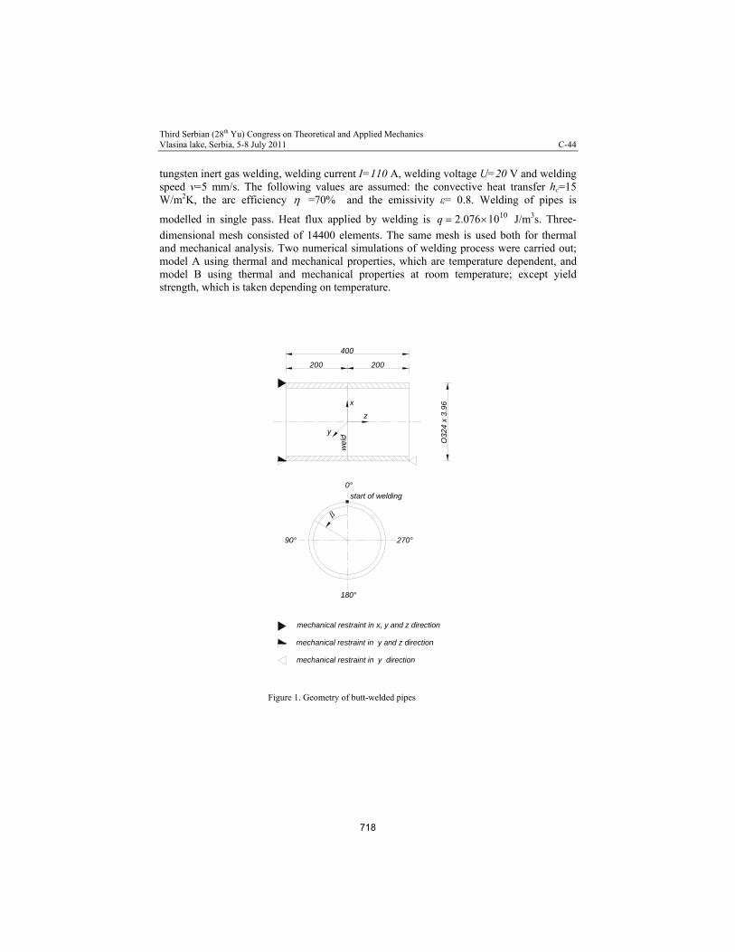
Third Serbian (28th Yu) Congress on Theoretical and Applied Mechanics Vlasina lake, Serbia, 5-8 July 2011 C-44
tungsten inert gas welding, welding current I=110 A, welding voltage U=20 V and welding speed v=5 mm/s. The following values are assumed: the convective heat transfer hc=15 W/m2K, the arc efficiency =70% and the emissivity ε= 0.8. Welding of pipes is
modelled in single pass. Heat flux applied by welding is 1010076.2 q J/m3s. Three-
dimensional mesh consisted of 14400 elements. The same mesh is used both for thermal and mechanical analysis. Two numerical simulations of welding process were carried out; model A using thermal and mechanical properties, which are temperature dependent, and model B using thermal and mechanical properties at room temperature; except yield strength, which is taken depending on temperature.
400
O32
4 x
3.96
0°
90° 270°
180°
start of welding
mechanical restraint in x, y and z direction
mechanical restraint in y and z direction
mechanical restraint in y direction
we
ld
y
x
z
200 200
Figure 1. Geometry of butt-welded pipes
718
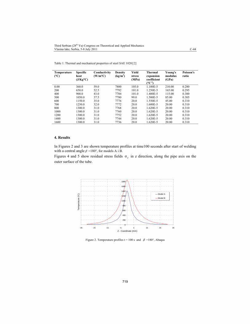
Third Serbian (28th Yu) Congress on Theoretical and Applied Mechanics Vlasina lake, Serbia, 5-8 July 2011 C-44
Table 1: Thermal and mechanical properties of steel SAE 1020 2]
Temperature (°C)
Specific heat (J/Kg°C)
Conductivity (W/m°C)
Density (kg/m3)
Yield stress (MPa)
Thermal expansion coefficient (°C-1)
Young's modulus (GPa)
Poisson's ratio
0.00 360.0 59.0 7800 105.0 1.100E-5 210.00 0.280 200 650.0 52.5 7792 101.0 1.250E-5 165.00 0.295 400 900.0 43.0 7784 101.0 1.400E-5 115.00 0.300 500 1050.0 37.5 7780 99.0 1.500E-5 85.00 0.305 600 1150.0 35.0 7776 20.0 1.550E-5 45.00 0.310 700 1250.0 32.0 7772 20.0 1.600E-5 20.00 0.310 800 1300.0 31.0 7768 20.0 1.620E-5 20.00 0.310 1000 1300.0 31.0 7760 20.0 1.620E-5 20.00 0.310 1200 1300.0 31.0 7752 20.0 1.620E-5 20.00 0.310 1400 1300.0 31.0 7744 20.0 1.620E-5 20.00 0.310 1600 1300.0 31.0 7736 20.0 1.620E-5 20.00 0.310
4. Results In Figures 2 and 3 are shown temperature profiles at time100 seconds after start of welding with a central angle =180°, for models A i B.
Figures 4 and 5 show residual stress fields zσ in z direction, along the pipe axis on the
outer surface of the tube.
0
200
400
600
800
1000
1200
1400
1600
1800
-35 -25 -15 -5 5 15 25 35
Z - Coordinate (mm)
Te
mp
era
ture
(°C
) Model A
Model B
Figure 2. Temperature profiles t = 100 s and =180°, Abaqus
719

Third Serbian (28th Yu) Congress on Theoretical and Applied Mechanics Vlasina lake, Serbia, 5-8 July 2011 C-44
0
200
400
600
800
1000
1200
1400
1600
1800
-35 -25 -15 -5 5 15 25 35
Z - Coordinate (mm)
Te
mp
era
ture
(°C
) Model A
Model B
Figure 3. Temperature profiles t = 100 s and =180°, Ansys
-80
-60
-40
-20
0
20
40
60
80
100
120
-200 -150 -100 -50 0 50 100 150 200
Z - Coordinate (mm)
Lo
ng
itud
ina
l re
sid
ua
l str
ess
z (M
Pa
)
Model A
Model B
Figure 4. Residual stresses zσ in z direction along inner surface
for =180°, model A and model B, Abaqus
-100
-80
-60
-40
-20
0
20
40
60
80
100
120
-200 -150 -100 -50 0 50 100 150 200
Z - Coordinate (mm)
Lo
ng
itud
ina
l re
sid
ua
l str
ess
z (M
Pa
)
Model A
Model B
Figure 5. Residual stresses zσ in z direction along inner surface
720
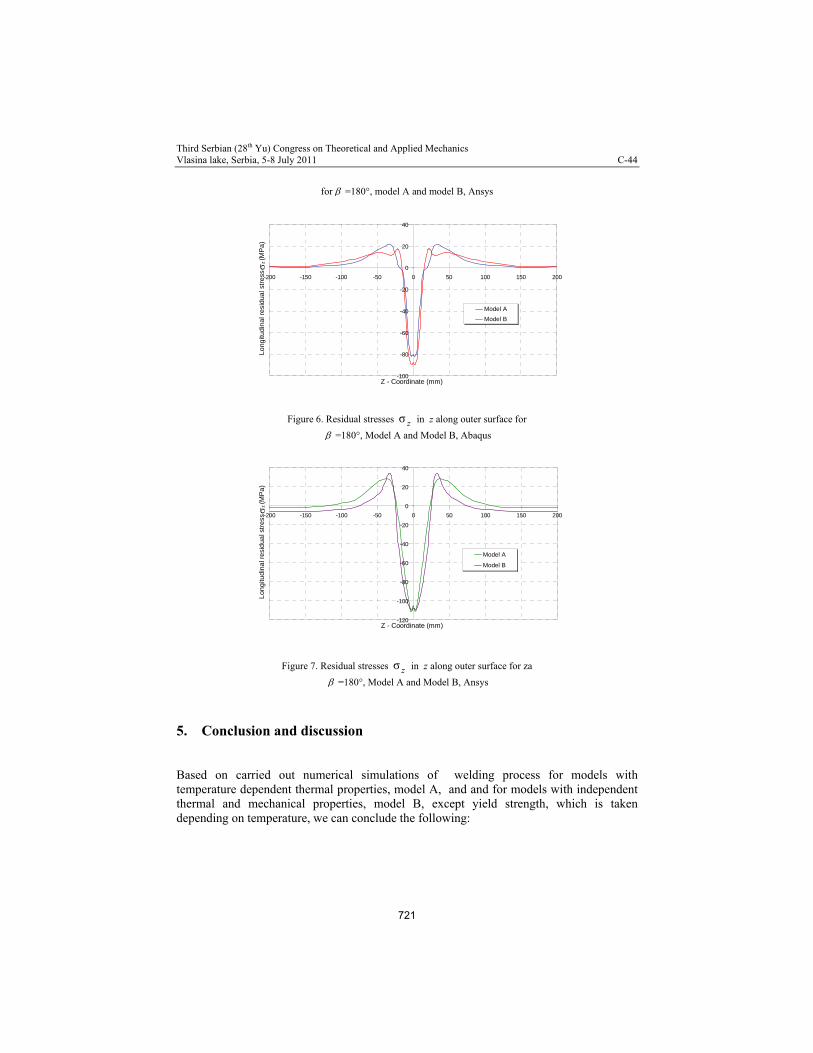
Third Serbian (28th Yu) Congress on Theoretical and Applied Mechanics Vlasina lake, Serbia, 5-8 July 2011 C-44
for =180°, model A and model B, Ansys
-100
-80
-60
-40
-20
0
20
40
-200 -150 -100 -50 0 50 100 150 200
Z - Coordinate (mm)
Lo
ng
itud
ina
l re
sid
ua
l str
ess
z (M
Pa
)
Model A
Model B
Figure 6. Residual stresses zσ in z along outer surface for
=180°, Model A and Model B, Abaqus
-120
-100
-80
-60
-40
-20
0
20
40
-200 -150 -100 -50 0 50 100 150 200
Z - Coordinate (mm)
Lo
ng
itud
ina
l re
sid
ua
l str
ess
z (M
Pa
)
Model A
Model B
Figure 7. Residual stresses zσ in z along outer surface for za
=180°, Model A and Model B, Ansys
5. Conclusion and discussion Based on carried out numerical simulations of welding process for models with temperature dependent thermal properties, model A, and and for models with independent thermal and mechanical properties, model B, except yield strength, which is taken depending on temperature, we can conclude the following:
721

Third Serbian (28th Yu) Congress on Theoretical and Applied Mechanics Vlasina lake, Serbia, 5-8 July 2011 C-44
Temperature fields for the case of numerical simulation of welding process of two steel tubes SAE 1020 in the welding zone, for models A and B, show significant discrepancies (Figures 2 and 3), which was confirmed with the parallel analysis in Abaqus and Ansys. Residual stresses zσ in direction of pipe axis, calculated along inner surface, are well
matched at models A and B, (Figures 4 and 5). Considerable difference among residual stresses zσ appear along outer surface (Figures 6 and 7), which was confirmed with the
parallel analysis in Abaqus and Ansys as well. According to the obtained values of residual stresses, we can conclude that the numerical simulation of the welding process is, using thermal and mechanical properties of steel materials at room temperature, except for yield strength which must be taken depending on the temperature, acceptable for a wide range of industries where less accuracy in the results of residual stresses and strain are required. In order to achieve more accurate residual stresses and strain, it is needed to know the thermal properties of materials at high temperatures.
References
[1] Zhu XK, Chao YJ (2002), Effects of temperature-dependent material properties on welding simulation,
Computers and Structures, 80, pp. 967-976. [2] Teng TL, Chang PH. (1998) ,Three-dimensional thermomechanical analysis of circumferentiallly welded thin-
waled pipes, International Journal of Pressure Vessels and Piping, 75, pp. 237-247. [3] Deng D, (2009), FEM prediction of welding residual stress and distortion in carbon steel considering phase
transformation effects. Materials and Design, 30, pp. 359-366. [4] Deng D, Liang W, Murakawa H. (2007), Determination of welding deformation in fillet –welded joint by
menas of numerical simulation and comparison with experimental measurements, Journal of Materials Processing Technology, 183, pp. 219-225.
[5] Deng D, Murakawa H., Liang W. (2007), Numerical simulation of welding distortion in large structures. Computer methods in applied mechanics and engineering, 196, pp. 4613-4627.
[6] Lee CH, Chang KH, (2008), Three-dimensional finite element simulation of residual stresses in circumferential welds of steel pipe diameter effects, Material Science and Engineering, 487, pp. 210-218.
[7] Peric M., Tonkovic Z., Karsaj I, (2010), Numerical analysis of residual stresses using a shell/3D modeling technique, Proceedings of the International Conference on Advances in Welding Science and Technology for Construction, Energy and Transportation AWST-2010, pp.75-80
[8] Stamenkovic D., Vasovic I.: Finite Element Analysis of Residual Stresses in Butt Welding Two Similar Plates, Scientific Technical Review, ISSN 1820-0206, 2009,Vol. LIX, No.1, pp.57-60.
[9] Peric M., Stamenkovic D., Milkovic V.: Comparison of residual stresses in butt-welded plates using software packages abaqus and ansys, Scientific Technical Review, ISSN 1820-0206, 2010,Vol.60,No.3-4, pp.22-26
[10] ABAQUS/Standard, User's guide and theoretical manual, Version 6.8, Hibbit, Karlsson & Serensen, Inc. (2008).
[11] Theory Reference for ANSYS and ANSYS Workbench, ANSYS Inc. Release 12.1
722