A numerical approach for modelling fracture in variably...
138
UNIVERSITÀ DEGLI STUDI DI PADOVA Dipartimento di ingegneria civile, edile e ambientale Technische Universität Carolo Wilhelmina zu Braunschweig Laurea Magistrale in Ingegneria Civile A numerical approach for modelling fracture in variably saturated porous media Relatore: Prof. Lorenzo SANAVIA Correlatore: Prof.ssa Laura DE LORENZIS Laureanda: Francesca MARCON 1058705 ANNO ACCADEMICO 2014-2015
Transcript of A numerical approach for modelling fracture in variably...

UNIVERSITÀ DEGLI STUDI DI PADOVA
Dipartimento di ingegneria civile, edile e ambientale
Technische Universität Carolo Wilhelmina zu Braunschweig
Laurea Magistrale in Ingegneria Civile
A numerical approach for modelling fracture
in variably saturated porous media
Relatore: Prof. Lorenzo SANAVIA
Correlatore: Prof.ssa Laura DE LORENZIS
Laureanda:
Francesca MARCON 1058705
ANNO ACCADEMICO 2014-2015


Ringraziamenti
In primis volevo ringraziare il Professor Lorenzo Sanavia per la pazienza
e il tempo dedicatomi alla realizzazione di questa tesi e la Professoressa
Laura de Lorenzis per l’aiuto e la collaborazione nel periodo a
Braunschweig.
I miei genitori per avermi permesso di intraprendere e ultimare
quest’avventura e mia sorella Michela per essermi stata vicina durante
tutto questo percorso.
Gli amici della compagnia di Silea, tutte le mie coinquiline, i miei
compagni di studi e tutti gli amici che in questi anni non solo universitari
hanno reso possibile questo traguardo.
Alberto per essermi stato vicino come solo lui sa fare supportandomi e
rubandomi sempre un sorriso.
Un grazie di cuore a tutti perché senza tutti voi ora non sarei qui a poter
festeggiare la fine di bellissimo percorso.


Index
Chapter 1 – Introduction 1
Chapter 2 – Theory of the porous media .................................................. 4
2.1. Governing equations for dynamic behaviour of saturated-
unsaturated porous media ..................................................................... 4
2.1.1. Introduction ............................................................................. 4
2.1.2. General assumption for behavior of porous media ................ 5
2.1.3. Description of skeleton deformation and fluid flow............... 6
2.1.4. Effective stress in partially saturated soils ............................. 7
2.1.5. Partial saturation and capillary pressure ................................. 8
2.1.6. Constitutive relation ............................................................. 10
2.1.7. Momentum equilibrium equations ....................................... 12
2.1.8 Water flow continuity equation ............................................. 13
2.1.9. Summary of governing equations ......................................... 14
2.1.10. Two simplifying approximations ....................................... 17
2.2. Discretization of governing equations ......................................... 19
2.2.1. Introduction ........................................................................... 19
2.2.2. Discretization in time ............................................................ 19
Chapter 3 – Modelling of the porous media ........................................... 31
3.1. Summary of the examples ........................................................... 31
3.2. Initial steps ................................................................................... 32
3.2.1. Step 1 .................................................................................... 32
3.2.2. Step 2 .................................................................................... 36
3.2.3. Step 3 .................................................................................... 39
3.2.4. Step 4 .................................................................................... 44
3.2.5. Step 5 .................................................................................... 51
3.3. Partially Saturated conditions ...................................................... 60
3.3.1. Explanation of the benchmark .............................................. 60
3.3.2. Implementation: results and validation ................................ 62
3.3.3. Conclusions........................................................................... 71
Chapter 4 - The phase-field description of dynamic brittle fracture ...... 72
4.1. Introduction to phase field ........................................................... 72
4.2. General remarks ........................................................................... 75
4.3. Model assumption in LEFM ........................................................ 76
4.4. Griffith’s theory of brittle fracture ............................................... 76
4.5. Phase-field approximation ........................................................... 79
4.4.1. Phase field theory ................................................................. 79
4.4.2. Numerical formulation ......................................................... 83
4.4.3. Time discretization and numerical implementation ................. 85
Chapter 5 – Examples and applications .................................................. 89
5.1. Description of the global model .................................................. 89
5.2. Examples and results ................................................................... 90

5.2.1. Exsiccation ............................................................................ 90
5.2.2. Traction on the top. Ten elements-column. ........................ 101
5.2.3. Traction on all the nodes on the top. 160 element-column 111
5.2.4. Traction on two the nodes on the top. 160 element-column
...................................................................................................... 119
Chapter 6 – Conclusions ....................................................................... 129
Bibliography .......................................................................................... 131

1
Chapter 1 – Introduction
This thesis, developed in cooperation with the Institute of Applied
Mechanics, Technische Universität Braunschweig (Germany), aspires to
couple a model of porous media with a phase field model for fracture.
In recent years, the interest in thermos-hydromechanics of partially
saturated porous media is increased and several mathematical models
were therefore implemented, neglecting however some relevant aspects
of the problem, which involves gas phase, water phase and the solid
matrix.
In this dissertation we take in account only two phases, i.e. the solid
matrix and water, omitting the effects of the gas in the mixture. The
implemented model consists in balance equations of mass, linear
momentum and energy, as well as of the appropriate constitutive
equations.
The macroscopic balance equations will be discretized both in space
(using the finite element method) and both in time.
The discretized equations in matrix form will be therefore solved by
means of a Newton-Raphson type procedure.
Some examples, simpler before and more and more complex and
complete later, will be carried out in order to validate the model step by
step, comparing it to analytical results or with the help of some
benchmarks.

2
From the case of fully saturated model, the dissertation will arrive to
discuss the case of a partially saturated model.
When the model of the porous media is completed and validated, it is
time to introduce the concept of phase field, for the study of the
development of the fracture in the material.
In order to briefly introduce the phase field model (better explained in
Chapter 4), we can describe it like a model where the fracture is
indicated with a scalar order parameter, which is able to change the
stiffness of the material, thanks to its link with the material properties.
In particular, the order parameter assumes the value zero where the
material is broken (and the stiffness will be consequently reduced), and
the value one for the undamaged material. At interface between broken
and undamaged material, the order parameter interpolates between zero
and one.
The Institute of Applied Mechanics, Technische Universität
Braunschweig (Germany), and in particular its Professor and Director,
Prof. Dr.-Ing. Laura De Lorenzis, supplied a Matlab code in which the
phase field model was implemented.
In this model, in addition to the displacement vector, the phase field
order parameter is treated as a supplementary nodal degree of freedom.
Usual linear shape functions can be used, together with four noded
element.

3
In every time step, the nonlinear coupled system of equations formed by
the discretized elasto-mechanincal field equations and the evolution
equation is solved using a Newton-Raphson algorithm.
The objective was therefore to introduce in this code the porous media
model, briefly descripted before, and to make the two fit together in
order to couple the two approaches and study the fracture in a porous
material.

4
Chapter 2 – Theory of the porous media
2.1. Governing equations for dynamic behaviour of saturated-unsaturated porous media
2.1.1. Introduction
Biot was the first who established the essence of the mathematical theory
governing the behavior of saturated porous media. He formulated the
solid-fluid interaction for linear elastic materials by a straightforward
physical approach.
Later, Zienkiewicz and Shiomi extended the Biot’s theory with large
strain and non-linear material behavior of saturated porous media.
This thesis uses a further expansion of the Biot’s theory where the
principle of effective stress is extended to unsaturated zones and the air
pressure is assumed to be zero.
The dynamic unsaturated context presents the most difficult situation and
the formulation is given in this case. The other phenomena (slow
consolidation or saturated behaviors) can be treated like special cases.
Throughout this thesis the stress is defined as tension positive and the
pressure as compression negative.

5
2.1.2. General assumption for behavior of porous media
Porous media are composed of a mass of solid grains separated by spaces
or voids. These voids are filled with air or water or both. The porous
media is dry when only air is present, it is saturated when only water is
present. When both water and air are present the porous media is said to
be partially saturated.
𝑆𝑤 , the degree of water saturation and 𝑆𝑎, the degree of air saturation are
defined as:
𝑆𝑤 =
𝑣𝑜𝑙𝑢𝑚𝑒 𝑜𝑓 𝑤𝑎𝑡𝑒𝑟
𝑣𝑜𝑙𝑢𝑚𝑒 𝑜𝑓 𝑣𝑜𝑖𝑑𝑠
𝑆𝑎 =𝑣𝑜𝑙𝑢𝑚𝑒 𝑜𝑓 𝑎𝑖𝑟
𝑣𝑜𝑙𝑢𝑚𝑒 𝑜𝑓 𝑣𝑜𝑖𝑑𝑠
(2.1)
If the porous media is dry, saturated or partially saturated the sum of 𝑆𝑤
and 𝑆𝑎 is always equal to unity:
𝑆𝑤 + 𝑆𝑎 = 1. (2.2)
The mechanics of porous media is described on a macroscopic scale so
that a continuum approach can be used in the analysis, assuming the
porous medium to be continuous everywhere, with air, water and solid
grains forming an overlapping continuum.
If the air flow is not significant and the air pressure is nearly uniform
over the domain considered, it may be assumed that the air pressure 𝑝𝑎 in
the unsaturated zones remains at atmospheric pressure, or:
𝑝𝑎 = 0 (2.3)
6
2.1.3. Description of skeleton deformation and fluid flow
A Cartesian coordinate system is used as a reference for all
displacements, velocities and accelerations. There are two different
description: Lagrangian and Eulerian. In the first one the attention is
focused on what is happening to a particular material with its initial
coordinate 𝑋. In the second one we concentrate on events at a particular
point 𝑥 in the space.
In small strain and small displacement analysis it makes no difference
which description is used. But if the finite deformation of the soil
skeleton is to be considered, a Lagrangian description is used for the
solid phase.
The displacement vector 𝑢 of a typical particle from its initial position 𝑋
to its position at time t is:
𝑢 = 𝑥 − 𝑋 (2.4)
Coupled problems in soil mechanics are generally focused on water
flow. is the water velocity relative to the solid phase and it is defined
as the rate of water flow across unit gross area of the solid-fluid
ensemble. The relative velocity of water is
(𝑛𝑆𝑤) .
𝑛 is the porosity of the solid which is defined as:
𝑛 =𝑣𝑜𝑙𝑢𝑚𝑒 𝑜𝑓 𝑣𝑜𝑖𝑑𝑠
𝑡𝑜𝑡𝑎𝑙 𝑣𝑜𝑙𝑢𝑚𝑒 𝑜𝑓 𝑠𝑜𝑖𝑙 (2.5)
The absolute velocity of water is:

7
= +
(𝑛𝑆𝑤) (2.6)
Where is the velocity of the solid phase.
2.1.4. Effective stress in partially saturated soils
For saturated soil Terzaghi, who introduced the concept of effective
stress, related it to the total stress 𝜎 and the water pressure 𝑝𝑤 as:
𝜎 = 𝜎′ + 𝑚 𝑝𝑤 (2.7)
Where 𝑚𝑇 = [1 1 1 0 0 0].
The principle of effective stress is extended to the unsaturated zones and
the Bishop’s law is adopted:
𝜎 = 𝜎′ + 𝑚 (2.8)
With:
= 𝜒 𝑝𝑤 + (1 − 𝜒) 𝑝𝑎 (2.9)
𝜒 is the Bishop’s parameter and it was suggested to be dependent on the
degree of water saturation, and other factors. can be treated like the
approximation of the pressure acting on the soil grains.
𝜒 may be approximated as:
𝜒 ≅ 𝑆𝑤 (2.10)
Substituting equations (2.10) and (2.1) into equation (2.9) gives:
8
= 𝑆𝑤 𝑝𝑤 + 𝑆𝑎 𝑝𝑎 (2.11)
Assuming the air pressure equals to zero, the equation becomes:
= 𝑆𝑤 𝑝𝑤 (2.12)
A modification of the equation (2.8) can be introduced to account for the
compressibility of the solid grains:
𝜎 = 𝜎′′ − 𝑚 𝛼 𝑝 (2.13)
𝜎′′ is the real effective stress.
For the concrete 𝛼 is in the range of 0.4 – 0.6 and in this case it is
important to take the effect of solid grain compressibility into account.
2.1.5. Partial saturation and capillary pressure
A liquid surface resists tensile forces because of the attraction between
adjacent molecules in the surface. The phenomenon of capillarity is
caused by such surface tension. The height of water column a soil can
thus support, depends on the capillarity pressure difference 𝑝𝑐 which is
defined as:
𝑝𝑐 = 𝑝𝑎 − 𝑝𝑤 (2.14)
The value of capillarity forces is inversely proportional to the size of soil
void at the air-water interface. There is great difference in the capillarity
tensions owing to the great difference in the particle size within sands
and clays. There can be very large capillarity tensions within clays, but
only very small capillarity tensions can exist within sands.

9
If the air pressure is zero, (2.14) can be written as :
𝑝𝑤 = −𝑝𝑐 (2.15)
Negative water pressures are thus maintained in the partially saturated
soils through the mechanism of capillarity forces. From equations (2.8),
(2.12) and (2.15) the effective stress can be written as:
𝜎′ = 𝜎 − 𝑚 𝑆𝑤 𝑝𝑐 (2.16)
The apparent cohesion 𝑆𝑤 𝑝𝑐 is a significant component of strength for
some soils in which the strength is proportional to the effective confining
stress.
Since the capillarity pressure is dependent on the size of soil void, for a
given granular material with specific void ratio and under isothermal
conditions we can assume that a unique function defines:
𝑝𝑐 = 𝑝𝑐(𝑆𝑤) (2.17a)
or
𝑆𝑤 = 𝑆𝑤(𝑝𝑐) (2.17b)
The permeability coefficient 𝑘𝑤 is, by similar arguments, again a unique
function.
𝑘𝑤 = 𝑘𝑤(𝑆𝑤) (2.18a)
or
𝑘𝑤 = 𝑘𝑤(𝑝𝑐) (2.18b)
10
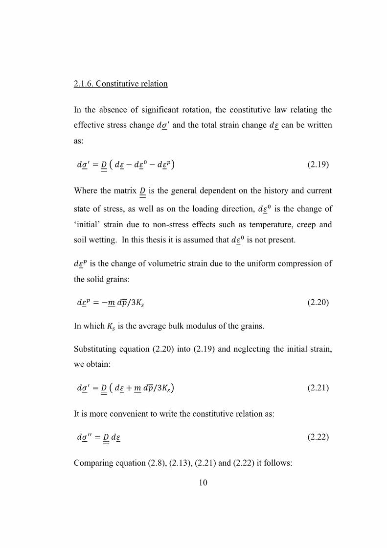
2.1.6. Constitutive relation
In the absence of significant rotation, the constitutive law relating the
effective stress change 𝑑𝜎′ and the total strain change 𝑑𝜀 can be written
as:
𝑑𝜎′ = 𝐷 ( 𝑑𝜀 − 𝑑𝜀0 − 𝑑𝜀𝑝) (2.19)
Where the matrix 𝐷 is the general dependent on the history and current
state of stress, as well as on the loading direction, 𝑑𝜀0 is the change of
‘initial’ strain due to non-stress effects such as temperature, creep and
soil wetting. In this thesis it is assumed that 𝑑𝜀0 is not present.
𝑑𝜀𝑝 is the change of volumetric strain due to the uniform compression of
the solid grains:
𝑑𝜀𝑝 = −𝑚 𝑑𝑝/3𝐾𝑠 (2.20)
In which 𝐾𝑠 is the average bulk modulus of the grains.
Substituting equation (2.20) into (2.19) and neglecting the initial strain,
we obtain:
𝑑𝜎′ = 𝐷 ( 𝑑𝜀 + 𝑚 𝑑𝑝/3𝐾𝑠) (2.21)
It is more convenient to write the constitutive relation as:
𝑑𝜎′′ = 𝐷 𝑑𝜀 (2.22)
Comparing equation (2.8), (2.13), (2.21) and (2.22) it follows:

11
𝛼 𝑚 = 𝑚 − 𝐷 𝑚
3 𝐾𝑠 (2.23)
Premultiplying equation (2.23) with 𝑚𝑇, we obtain:
𝛼 = 1 −𝑚𝑇 𝐷 𝑚
9 𝐾𝑠 (2.24)
In this case the material is isotropic so the quantity of 𝑚𝑇 𝐷 𝑚 is equal to
9 𝐾𝑠, and 𝐾𝑠 is the bulk modulus of the overall soil mixture. Equation
(2.24) can be simplified as:
𝛼 = 1 −𝐾𝑡
𝐾𝑠 (2.25)
For small strain analysis, the change of total strain 𝑑𝜀 is related to the
change of displacement 𝑑𝑢 of the soil skeleton as:
𝑑𝜀𝑖𝑗 = ( 𝑑𝑢𝑖,𝑗 + 𝑑𝑢𝑗,𝑖)/2 (2.26a)
or
𝑑𝜀 = 𝐿 𝑑𝑢 (2.26b)
And the differential operator 𝐿𝑇 is defined as:

12
𝐿𝑇 =
[
𝜕
𝜕𝑥0 0
0𝜕
𝜕𝑦0
0 0𝜕
𝜕𝑧𝜕
𝜕𝑦
𝜕
𝜕𝑥0
0𝜕
𝜕𝑧
𝜕
𝜕𝑦
𝜕
𝜕𝑧0
𝜕
𝜕𝑥]
(2.27)
2.1.7. Momentum equilibrium equations
Assuming that the coordinate system moves with the solid phase the
convective acceleration is applied only to the fluid. For a unit volume of
the soil mixture, the overall equilibrium equation relates the total stress 𝜎
and the body force 𝑏 to the acceleration of the soil skeleton and the
relative acceleration of water in this form:
𝐿𝑇𝜎 + 𝜌 𝑏 = 𝜌 + 𝜌𝑤 𝑛 𝑆𝑤 𝐷
𝐷𝑡(
𝑛 𝑆𝑤) (2.28)
𝜌𝑤 is the density of the water and 𝜌 is the density of the soil mixture
written as:
𝜌 = 𝜌𝑠 (1 − 𝑛) + 𝜌𝑤 𝑛 𝑆𝑤 (2.29)
𝜌𝑠 is the density of the solid grain.
In the case of water passing through soil, the validity of Darcy law is
assumed. For a unit volume of water, the Darcy law in the generalized
form can be written as:

13
𝑘𝑤−1 = −∇𝑝𝑤 + 𝑝𝑤 (𝑏 −
𝐷
𝐷𝑡) (2.30)
𝑘𝑤 is the dynamic permeability matrix of water. For isotropic case it is
conveniently replaced by a single 𝑘𝑤 value. is the actual velocity of
water as indicated in equation 6 and the acceleration of water is given as:
𝐷
𝐷𝑡= +
𝐷
𝐷𝑡(
𝑛 𝑆𝑤) (2.31)
Since the air pressure has been assumed to be zero, the equation (2.30) is
not need in the present analysis approach.
2.1.8 Water flow continuity equation
For a unit volume of soil mixture, the rate of water inflow is given by:
−∇𝑇 (2.32)
There are five factors that contribute to the change of water stored in the
unit volume of the solid-fluid ensemble:
1. Volumetric strain of the soil skeleton:
𝑚𝑇 𝜕𝜀
𝜕𝑡 (2.33a)
2. Compressive volumetric strain of the grain due to pressure changes:
(1−𝑛)
𝐾𝑠 𝜕𝑝
𝜕𝑡 (2.33b)
3. Compressive volumetric strain of water:
𝑛 𝑆𝑤
𝐾𝑤 𝜕𝑝𝑤
𝜕𝑡 (2.33c)
4. Increase of water storage due to saturation changes:

14
𝑛 𝜕𝑆𝑤
𝜕𝑡= 𝑛
𝜕𝑆𝑤
𝜕𝑝𝑤
𝜕𝑝𝑤
𝜕𝑡= 𝐶𝑠
𝜕𝑝𝑤
𝜕𝑡 (2.33d)
Where 𝐶𝑠 is the specific moisture capacity, which can be evaluated from
𝑆𝑤 − 𝑝𝑤 curves as 𝑛 𝜕𝑆𝑤
𝜕𝑝𝑤.
5. Compressive volumetric strain of grain due to effective stress:
−1
3𝐾𝑠𝑚𝑇 𝜕𝜎′
𝜕𝑡= −
1
3𝐾𝑠𝑚𝑇𝐷
𝜕𝜀
𝜕𝑡− 𝑚𝑇𝐷 𝑚
1
(3𝐾𝑠)2
𝜕𝑝
𝜕𝑡 (2.33e)
The final continuity equation for water flow becomes:
−∇𝑇 = 𝑛 𝑆𝑤
𝐾𝑤 𝜕𝑝𝑤
𝜕𝑡+ 𝐶𝑠
𝜕𝑝𝑤
𝜕𝑡+ 𝑆𝑤 (𝑚𝑇 −
𝑚𝑇𝐷
3𝐾𝑠)
𝜕𝜀
𝜕𝑡+ 𝑆𝑤 [
(1−𝑛)
𝐾𝑠+
− 𝑚𝑇𝐷 𝑚 1
(3𝐾𝑠)2]
𝜕𝑝
𝜕𝑡 (2.34)
Using the definition of 𝑝 in the equation (2.12) an of 𝛼 in equation
(2.23), equation (2.34) becomes:
−∇𝑇 = 𝑛 𝑆𝑤
𝐾𝑤 𝜕𝑝𝑤
𝜕𝑡+ 𝐶𝑠
𝜕𝑝𝑤
𝜕𝑡+ 𝑆𝑤𝛼 𝑚𝑇 𝜕𝜀
𝜕𝑡+ 𝑆𝑤
(𝛼−𝑛)
𝐾𝑠(𝑆𝑤 +
𝐶𝑠
𝑛𝑝𝑤)
𝜕𝑝𝑤
𝜕𝑡
(2.35)
This is a general equation for continuity of water flow through a partially
saturated porous medium.
2.1.9. Summary of governing equations
1. Equilibrium of the soil mixture:
𝐿𝑇𝜎 + 𝜌 𝑏 = 𝜌 + 𝜌𝑤 𝑛 𝑆𝑤 𝐷
𝐷𝑡(
𝑛 𝑆𝑤) (2.36a)
2. Equilibrium of water:
𝑘𝑤−1 = −∇𝑝𝑤 + 𝑝𝑤 (𝑏 − −
𝐷
𝐷𝑡(
𝑛 𝑆𝑤)) (2.36b)
3. Continuity of water flow:

15
−∇𝑇 = 𝑛 𝑆𝑤
𝐾𝑤
𝜕𝑝𝑤
𝜕𝑡+ 𝐶𝑠
𝜕𝑝𝑤
𝜕𝑡+ 𝑆𝑤𝛼 𝑚𝑇
𝜕𝜀
𝜕𝑡+
+𝑆𝑤(𝛼−𝑛)
𝐾𝑠(𝑆𝑤 +
𝐶𝑠
𝑛𝑝𝑤)
𝜕𝑝𝑤
𝜕𝑡 (2.36c)
4. The real ‘effective stress’:
𝜎 = 𝜎′′ − 𝑚 𝛼 𝑆𝑤 𝑝𝑤 (2.36d)
5. Constitutive relation:
𝑑𝜎′′ = 𝐷 𝑑𝜀 (2.36e)
6. Incremental strain:
𝑑𝜀 = 𝐿 𝑑𝑢 (2.36f)
7. Partial saturation relationships:
𝑆𝑤 = 𝑆𝑤(𝑝𝑐), 𝑘𝑤 = 𝑘𝑤(𝑝𝑐) 𝑎𝑛𝑑 𝐶𝑠 = 𝑛 𝜕𝑆𝑤
𝜕𝑝𝑤 (2.36g)
The above system of equations is the generalized Biot formulation for
dynamic behavior of saturated-unsaturated porous media. It can be
solved incrementally for most problems with appropriate boundary and
initial conditions such as:
Boundary conditions
a. Prescribed displacement
𝑢 = 𝑢 𝑜𝑛 𝛤𝑢 𝑎𝑡 𝑡 ≥ 0 (2.37)
b. Prescribed traction
𝑡 = 𝑡 𝑜𝑛 𝛤𝑡 𝑎𝑡 𝑡 ≥ 0 (2.38a)
i.e.
𝑙𝑇 𝜎 = 𝑡 𝑜𝑛 𝛤𝑡 𝑎𝑡 𝑡 ≥ 0 (2.38b)
In which the matrix 𝑙 is related to the unit normal vector
𝑛 = [𝑛𝑥 , 𝑛𝑦 , 𝑛𝑧]𝑇 by

16
𝑙 =
[ 𝑛𝑥 0 00 𝑛𝑦 0
0 0 𝑛𝑧
𝑛𝑦 𝑛𝑥 0
0 𝑛𝑧 𝑛𝑦
𝑛𝑧 0 𝑛𝑥]
(2.38c)
c. Prescribed water flow:
= 𝑜𝑛 𝛤𝑤 𝑎𝑡 𝑡 ≥ 0 (2.39a)
or from the equation (2.33b) it is given that:
𝑘𝑤 (−∇𝑝𝑤 + 𝑝𝑤 (𝑏 − − 𝐷
𝐷𝑡(
𝑛 𝑆𝑤))) = (2.39b)
d. Prescribed water pressure:
𝑝𝑤 = 𝑝𝑤 𝑜𝑛 𝛤𝑝𝑤
𝑎𝑡 𝑡 ≥ 0 (2.40)
Initial conditions
𝑢 = 𝑢0 (2.41a)
= 0 𝑖𝑛 𝛺 𝑎𝑛𝑑 𝑜𝑛 𝛤 𝑎𝑡 𝑡 = 0 (2.41b)
𝑝𝑤 = 𝑝𝑤0 (2.41c)
There are nine variables in the system (2.36). They are named 𝑢, 𝑤, 𝜀,
𝜎, 𝜎′′, 𝑆𝑤 , 𝐾𝑤 and 𝐶𝑠. A direct numerical solution to equations (2.36)
can be obtained by taking 𝑢 and 𝑤 as primary variables with other
variables eliminated. Solving these equations for nonlinear dynamic
problems can be very expensive. Therefore, under certain conditions, an

17
approximation to the system (2.36) is useful and indeed more
economical for the practical use.
2.1.10. Two simplifying approximations
Partially saturated dynamic u-p formulation
When the relative acceleration of the water with respect to the soil
skeleton is not significant, the variable 𝑤 can be eliminated by dropping
the acceleration terms associated with 𝑤 on the assumption that: 𝐷
𝐷𝑡 ≪ 𝑜𝑟
𝐷
𝐷𝑡 (
𝑛 𝑆𝑤) ≪ (2.42)
For most problems in earthquake response analysis, this approximation is
sufficiently accurate. The equation system (2.36) can now be reduced by
eliminating between (2.36b) and (2.36c) to:
𝐿𝑇𝜎 + 𝜌 𝑏 = 𝜌 (2.43a)
∇𝑇 [𝑘𝑤 (∇𝑝𝑤 − 𝜌𝑤(𝑏 − ))] = 𝑛 𝑆𝑤
𝐾𝑤 𝜕𝑝𝑤
𝜕𝑡+ 𝐶𝑠
𝜕𝑝𝑤
𝜕𝑡+ 𝑆𝑤𝛼 𝑚𝑇 𝜕𝜀
𝜕𝑡+
+𝑆𝑤(𝛼−𝑛)
𝐾𝑠(𝑆𝑤 +
𝐶𝑠
𝑛𝑝𝑤)
𝜕𝑝𝑤
𝜕𝑡 (2.43b)
𝜎 = 𝜎′′ − 𝑚 𝛼 𝑆𝑤 𝑝𝑤 (2.43c)
𝑑𝜎′′ = 𝐷 𝑑𝜀 (2.43d)
𝑑𝜀 = 𝐿 𝑑𝑢 (2.43e)

18
𝑆𝑤 = 𝑆𝑤(𝑝𝑐), 𝑘𝑤 = 𝑘𝑤(𝑝𝑐) 𝑎𝑛𝑑 𝐶𝑠 = 𝑛 𝜕𝑆𝑤
𝜕𝑝𝑤 (2.43f)
This is the dynamic u-p formulation partially saturated porous media,
where the displacement 𝑢 and water pressure 𝑝𝑤 are taken as primary
variables.
Partially saturated consolidation form
This is the case developed in this thesis. The problem is very slow and
all the acceleration forces are found to be negligible:
𝐷
𝐷𝑡 (
𝑛 𝑆𝑤) → 0 𝑎𝑛𝑑 → 0 (2.44)
The consolidation equations are obtained:
𝐿𝑇𝜎 + 𝜌 𝑏 = 0 (2.45a)
∇𝑇[𝑘𝑤(∇𝑝𝑤 − 𝜌𝑤𝑏)] = 𝑛 𝑆𝑤
𝐾𝑤
𝜕𝑝𝑤
𝜕𝑡+ 𝐶𝑠
𝜕𝑝𝑤
𝜕𝑡+ 𝑆𝑤𝛼 𝑚𝑇
𝜕𝜀
𝜕𝑡+
+𝑆𝑤(𝛼−𝑛)
𝐾𝑠(𝑆𝑤 +
𝐶𝑠
𝑛𝑝𝑤)
𝜕𝑝𝑤
𝜕𝑡 (2.45b)
𝜎 = 𝜎′′ − 𝑚 𝛼 𝑆𝑤 𝑝𝑤 (2.45c)
𝑑𝜎′′ = 𝐷 𝑑𝜀 (2.45d)
𝑑𝜀 = 𝐿 𝑑𝑢 (2.45e)
19
𝑆𝑤 = 𝑆𝑤(𝑝𝑐), 𝑘𝑤 = 𝑘𝑤(𝑝𝑐) 𝑎𝑛𝑑 𝐶𝑠 = 𝑛 𝜕𝑆𝑤
𝜕𝑝𝑤 (2.45f)
There are the same equations of the system (2.44) but with terms
containing omitted.
2.2. Discretization of governing equations
2.2.1. Introduction
In Section 2.1, the governing equations for the coupled problem of
saturated-unsaturated flow in deforming porous media have been
presented.
Because of the eventually complex geometry and arbitrary nonlinearity
in these kind of problems, the use of the finite element method is the
most recommended, and is therefore used in this thesis.
In this Section, the numerical solution to the governing equations of
static behaviour of saturated-unsaturated porous media is discussed.
First, the time discretization and the iterative Newton-Raphson
procedure is described. Then the finite element method is applied to the
generalized Biot equations for the spatial discretization.
2.2.2. Discretization in time
Generally, a boundary value problem can be represented as:

20
𝐴(𝑢) = 𝐶 𝑢 + 𝑝 = 0 𝑖𝑛 Ω (2.46a)
and
𝐵(𝑢) = 𝐷 𝑢 + 𝑞 = 0 𝑜𝑛 𝛤 (2.46b)
Where C and D are linear or nonlinear differential operators, p and q are
functions defined in the domain Ω and on the boundary 𝛤 and u is the
exact solution to the governing equation (2.46a) subject to the boundary
condition (2.46b).
Due to the impossibility of finding the exact solution, some
approximations must be done.
This is the reason for the introduction of the Weighted Residual Method,
which assumes that a solution can be approximated analytically or
piecewise analytically. In general, a solution of the problem can be
expressed as a linear combination of a base set of functions where the
coefficients are determined by a chosen method, and the method
attempts to minimize the approximation error.
Indeed, the approximation 𝑢∗ , substituted into (2.46a) and (2.46b),
usually do not satisfy them with the creation of a residual in the domain:
𝑅Ω = 𝐴(𝑢∗) = 𝐶 𝑢 + 𝑝 = 0 𝑖𝑛 Ω (2.47a)
and
𝑅Ω = 𝐵(𝑢∗) = 𝐷 𝑢 + 𝑞 = 0 𝑜𝑛 𝛤 (2.47b)
The residuals can be made zero in some weighted sense writing:

21
∫ Ω 𝑊𝑇𝑅Ω 𝑑Ω + ∫ Γ 𝑊𝑇𝑅𝛤 𝑑𝛤 (2.48)
or
∫ Ω 𝑊𝑇 (𝐶 𝑢 + 𝑝)𝑑Ω + ∫ Γ 𝑊𝑇( 𝐷 𝑢 + 𝑞) 𝑑𝛤 (2.49)
where the weighted functions 𝑊 and 𝑊 can be, in general, chosen
independently.
In what follows, the weighted residual method is applied in the case of
the partially saturated dynamic u-p formulation of (2.43).
Applying the integral equation (2.49) to the equilibrium equation (2.43a)
and the boundary condition (2.38b), we obtain:
∫ Ω 𝑊𝑇(𝐿𝑇𝜎 + 𝜌𝑏 − 𝜌)𝑑Ω + ∫ Γ 𝑊𝑇(𝑙𝑇 𝜎 − 𝑡)𝑑𝛤 = 0 (2.50)
The boundary condition (2.37) of 𝑢 = 𝑢 on 𝛤𝑢 is satisfied by the choice
of the approximation of 𝑢.
By using the Green’s theorem, the first term of the equation (2.50)
becomes:
−∫ Ω ( 𝐿 𝑊 )𝑇𝜎 𝑑Ω + ∫
𝛤𝑢+𝛤𝑡𝑊
𝑇𝑙𝑇𝜎 𝑑𝛤 (2.51)
Forcing the weighting functions to be like:
𝑊 = 0 𝑜𝑛 𝛤𝑢 (2.52a)
𝑊 = −𝑊 𝑜𝑛 𝛤𝑡 (2.52b)

22
the equation (2.50) is reduced to:
∫ Ω ( 𝐿 𝑊 )𝑇𝜎 𝑑Ω + ∫ Ω 𝑊𝑇𝜌 𝑑Ω = ∫ Ω 𝑊𝑇𝜌𝑏 𝑑Ω + ∫ Γ 𝑊
𝑇𝑡 𝑑𝛤
(2.53)
The continuity equation of water flow can be rewritten substituting
equation (2.43e) into (2.43b) as:
∇𝑇[−𝑘𝑤 ∇ 𝑝𝑤 + 𝑘𝑤 𝜌𝑤 ( 𝑏 − )] + 𝑆𝑤 𝛼 𝑚𝑇𝐿 + 1
𝑄∗ = 0 (2.54)
where
1
𝑄∗= 𝐶𝑠 + 𝑛
𝑆𝑤
𝐾𝑤+ 𝑆𝑤
( 𝛼−𝑛 )
𝐾𝑠 ( 𝑆𝑤 +
𝐶𝑠
𝑛 𝑝𝑤) (2.55)
As regards the boundary condition (2.39b), it can be simplified using the
assumption (2.44) for the dynamic u-p formulation. The result is:
𝑘𝑤 [ −∇ 𝑝𝑤 + 𝜌𝑤( 𝑏 − ) ] = 𝑜𝑛 𝛤𝑤 (2.56)
It is possible now to apply the weighted residual method to the equations
(2.54) and (2.56), obtaining:
∫ 𝑊∗𝑇 ∇𝑇[−𝑘𝑤 ∇ 𝑝𝑤 + 𝑘𝑤 𝜌𝑤 ( 𝑏 − )] + 𝑆𝑤 𝛼 𝑚𝑇𝐿 + 1
𝑄∗ 𝑑Ω +
Ω
+ ∫ Γ 𝑊∗𝑇
[−𝑘𝑤∇ 𝑝𝑤 + 𝑘𝑤 𝜌𝑤( 𝑏 − ) − ]𝑇𝑛 𝑑𝛤 = 0 (2.57)
where 𝑊∗ and 𝑊∗ are arbitrary weighting functions.
The boundary condition (2.40) of 𝑝𝑤 = 𝑝𝑤 on 𝛤𝑤 is satisfied by the
choice of the approximation of 𝑝𝑤.

23
By applying the Green’s theorem to the first term of the first integral of
the equation (2.57), and limiting the choice of the weighting functions so
that:
𝑊∗ = 0 𝑜𝑛 𝛤𝑝 (2.58a)
𝑊∗ = −𝑊∗ 𝑜𝑛 𝛤𝑢 𝑜𝑛 𝛤𝑤 (2.58b)
the equation (2.57) is now written as:
∫ −(∇ 𝑊∗)𝑇[−𝑘𝑤 ∇ 𝑝𝑤 + 𝑘𝑤 𝜌𝑤 ( 𝑏 − )] + 𝑊∗𝑇𝑆𝑤 𝛼 𝑚𝑇𝐿 +
Ω
+ 𝑊∗𝑇 1
𝑄∗ 𝑑Ω + ∫ 𝑊∗𝑇
𝑇𝑛
𝛤𝑤 𝑑𝛤 = 0 (2.59)
At the end the equations weighted are:
∫ (𝐿𝑊∗)𝑇
Ω𝜎 𝑑Ω − ∫ (𝑊∗)
𝑇𝜌𝑏 𝑑Ω
Ω− ∫ Γ 𝑊
𝑇𝑡 𝑑𝛤 = 0 (2.60a)
∫ −(∇ 𝑊∗)𝑇[−𝑘𝑤 ∇ 𝑝𝑤 + 𝑘𝑤 𝜌𝑤 𝑏] + 𝑊∗𝑇𝑆𝑤 𝛼 𝑚𝑇𝐿 +
Ω
+ 𝑊∗𝑇 1
𝑄∗ 𝑑Ω + ∫ 𝑊∗𝑇
𝑇𝑛
𝛤𝑤 𝑑𝛤 = 0 (2.60b)
With:
𝜎 = 𝜎′ + 𝑆𝑤 𝛼 𝑚 (2.61a)
𝜌 = 𝜌𝑠(1 − 𝑛) + 𝑛𝑆𝑤 (2.61b)
It is assumed that the differential equations are to be satisfied at each
discrete time station.
The derived terms are substituted with their incremental ratio in the
following way:

24
= (𝑑𝑢
𝑑𝑡)
𝑛+1=
𝑢𝑛+1
−𝑢𝑛
∆𝑡 (2.62a)
= (𝑑𝑝
𝑑𝑡)
𝑛+1=
𝑝𝑛+1
−𝑝𝑛
∆𝑡 (2.62b)
𝑛+1 =𝑆𝑛+1−𝑆𝑛
∆𝑡 (2. 62c)
Eq. 2.70c can be written as:
𝑛+1 =𝜕𝑆
𝜕𝑝 (2.62d)
where the suffix ‘w’ is now omitted for simplicity.
Inserting the (2.62a) and (2.62b) into the equations (2.60a) and (2.60b),
the result is:
∫ (𝐿𝑊∗)𝑇
Ω𝜎 ′𝑛+1𝑑Ω − ∫ (𝐿𝑊∗)
𝑇
𝑆𝑤 𝛼 𝑚𝑝𝑛+1
𝑑ΩΩ
− ∫ (𝑊∗)𝑇[(1 −
Ω
𝑛)𝜌𝑠 + 𝑛𝑆𝑤𝑛+1𝜌𝑤]𝑏 𝑑Ω − ∫ Γ 𝑊
𝑇𝑡 𝑑𝛤 = 0 (2.63a)
∇𝑡 ∫ (∇ 𝑊∗)𝑇𝑘𝑤 ∇ 𝑝𝑤𝑛+1
𝑑Ω − ∇𝑡 ∫ (∇ 𝑊∗)𝑇𝑘𝑤 𝜌𝑤 𝑏 𝑑Ω +
ΩΩ
∫ 𝑊∗𝑇𝑆𝑤 𝛼 𝑚𝑇𝐿 𝑢𝑛+1
𝑑Ω −Ω
∫ 𝑊∗𝑇𝑆𝑤 𝛼 𝑚𝑇𝐿 𝑢𝑛 𝑑Ω
Ω+∫ 𝑊∗𝑇 1
𝑄∗𝑝
𝑛+1Ω 𝑑Ω − ∫ 𝑊∗𝑇 1
𝑄∗𝑝
𝑛Ω 𝑑Ω +
∇𝑡 ∫ 𝑊∗𝑇 𝑇𝑛
𝛤𝑤 𝑑𝛤 = 0 (2.63b)
The system of equation now obtained is a non-linear system. To be
solved, it needs some iterative procedure. We decided to use the
Newton-Raphson method.

25
Eq. (2.63a) can be written as 𝑅1 (𝑢𝑛+1
, 𝑝𝑛+1
) and Eq. (2.63b) as
𝑅2 (𝑢𝑛+1
, 𝑝𝑛+1
).
The next passage is the differentiation of the two equations of the (2.63),
in order to obtain a system with the following structure:
[(
𝜕𝑅1
𝜕𝑢𝑛+1)(𝑖)
∆𝑢𝑛+1(𝑖+1) (
𝜕𝑅1
𝜕𝑝𝑛+1)(𝑖)
∆𝑝𝑛+1(𝑖+1)
(𝜕𝑅2
𝜕𝑢𝑛+1)(𝑖)
∆𝑢𝑛+1(𝑖+1) (
𝜕𝑅2
𝜕𝑝𝑛+1)(𝑖)
∆𝑝𝑛+1(𝑖+1)
] = − [𝑅1
(𝑖)
𝑅2(𝑖)
] (2.64)
where the index (i) identifies the respective Newton-Raphson iteration.
Each term of the matrix in (2.64) is reported below:
𝜕𝑅1
𝜕𝑢𝑛+1∆𝑢𝑛+1 = ∫ (𝐿𝑊∗)
𝑇
Ω
𝜕𝜎′𝑛+1
𝜕𝜀𝑛+1
𝜕𝜀𝑛+1
𝜕𝑢𝑛+1∆𝑢𝑛+1𝑑Ω = ∫ (𝐿𝑊∗)
𝑇
Ω
𝜕𝜎′𝑛+1
𝜕𝜀𝑛+1𝐿 ∆𝑢𝑛+1𝑑Ω
( 2.65)
𝜕𝑅1
𝜕𝑝𝑛+1∆𝑝𝑛+1 = −∫ (𝐿𝑊∗)
𝑇 𝜕𝑆𝑤
𝜕𝑝𝑛+1 𝛼 𝑚 ∆𝑝𝑛+1 𝑝
𝑛+1 𝑑Ω
Ω−
∫ (𝐿𝑊∗)𝑇𝑆𝑤𝑛+1
𝛼 𝑚 𝜕𝑝
𝑛+1
𝜕𝑝𝑛+1
∆𝑝𝑛+1 𝑑ΩΩ
+ −∫ (𝑊∗)𝑇 𝜕𝑆𝑤
𝜕𝑝𝑛+1Ω𝑛𝜌𝑤𝑏 ∆𝑝𝑛+1 𝑑Ω (2.66)
𝜕𝑅2
𝜕𝑢𝑛+1∆𝑢𝑛+1 = ∫ 𝑊∗𝑇𝑆𝑤 𝛼 𝑚𝑇𝐿
𝜕𝑢𝑛+1
𝜕𝑢𝑛+1
∆𝑢𝑛+1 𝑑ΩΩ
(2.67)
𝜕𝑅2
𝜕𝑝𝑛+1∆𝑝𝑛+1 = ∆𝑡 ∫ (∇ 𝑊∗)
𝑇 𝜕𝑘𝑤
𝜕𝑝𝑛+1
∆𝑝𝑛+1 ∇ 𝑝𝑤𝑛+1𝑑Ω
Ω+
∆𝑡 ∫ (∇ 𝑊∗)𝑇 𝜕𝑝
𝑛+1
𝜕𝑝𝑛+1
𝑘𝑤∆𝑝𝑛+1 𝑑ΩΩ
+ −∆𝑡 ∫ (∇ 𝑊∗)𝑇 𝜕𝑘𝑤
𝜕𝑝𝑛+1
∆𝑝𝑛+1 𝜌𝑤 𝑏 𝑑ΩΩ
+
∫ 𝑊∗𝑇 𝜕𝑆𝑤
𝜕𝑝𝑛+1∆𝑝𝑛+1 𝛼 𝑚𝑇𝐿 𝑢
𝑛+1 𝑑Ω +
Ω
−∫ 𝑊∗𝑇 𝜕𝑆𝑤
𝜕𝑝𝑛+1 ∆𝑝𝑛+1 𝛼 𝑚𝑇𝐿 𝑢
𝑛 𝑑Ω
Ω+∫ 𝑊∗𝑇
𝜕1
𝑄∗
𝜕𝑝𝑛+1∆𝑝𝑛+1 𝑝
𝑛+1Ω 𝑑Ω +
+∫ 𝑊∗𝑇 1
𝑄∗
𝜕𝑝𝑛+1
𝜕𝑝𝑛+1
Ω ∆𝑝𝑛+1 𝑑Ω − ∫ 𝑊∗𝑇
𝜕1
𝑄∗
𝜕𝑝𝑛+1∆𝑝𝑛+1 𝑝
𝑛Ω 𝑑Ω (2.68)
26
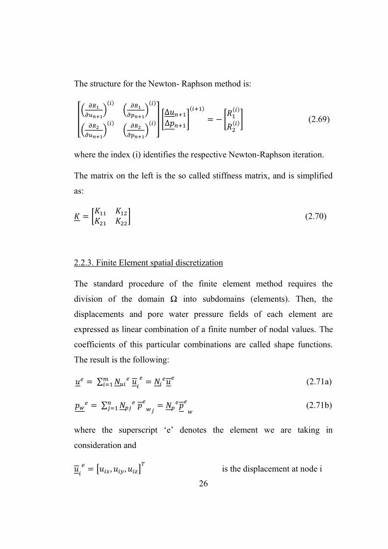
The structure for the Newton- Raphson method is:
[(
𝜕𝑅1
𝜕𝑢𝑛+1)
(𝑖)
(𝜕𝑅1
𝜕𝑝𝑛+1)
(𝑖)
(𝜕𝑅2
𝜕𝑢𝑛+1)
(𝑖)
(𝜕𝑅2
𝜕𝑝𝑛+1)
(𝑖)] [
∆𝑢𝑛+1
∆𝑝𝑛+1]
(𝑖+1)
= − [𝑅1
(𝑖)
𝑅2(𝑖)
] (2.69)
where the index (i) identifies the respective Newton-Raphson iteration.
The matrix on the left is the so called stiffness matrix, and is simplified
as:
𝐾 = [𝐾11 𝐾12
𝐾21 𝐾22] (2.70)
2.2.3. Finite Element spatial discretization
The standard procedure of the finite element method requires the
division of the domain Ω into subdomains (elements). Then, the
displacements and pore water pressure fields of each element are
expressed as linear combination of a finite number of nodal values. The
coefficients of this particular combinations are called shape functions.
The result is the following:
𝑢𝑒 = ∑ 𝑁𝑢𝑖𝑒 𝑢
𝑖
𝑒= 𝑁𝑖
𝑒𝑢𝑒𝑚
𝑖=1 (2.71a)
𝑝𝑤𝑒 = ∑ 𝑁𝑝𝑗
𝑒 𝑝𝑒
𝑤𝑗= 𝑁𝑝
𝑒𝑝𝑒
𝑤
𝑛𝑗=1 (2.71b)
where the superscript ‘e’ denotes the element we are taking in
consideration and
𝑢𝑖
𝑒= [𝑢𝑖𝑥 , 𝑢𝑖𝑦 , 𝑢𝑖𝑧]
𝑇 is the displacement at node i

27
𝑢𝑒
= [𝑢1
𝑒𝑇
… . 𝑢𝑖
𝑒𝑇
… . 𝑢𝑚
𝑒𝑇
]𝑇
is the nodal displacement
vector
𝑝𝑒
𝑤𝑗 is the water pressure at node j
𝑝𝑒
𝑤= [ 𝑝𝑤1
𝑒 … . 𝑝𝑤𝑗𝑒 … . 𝑝𝑤𝑚
𝑒 ]𝑇 is the nodal water pressure
vector
m is the number of nodes per
element for the displacement
shape function
n is the number of nodes per
element for the water pressure
shape function
𝑁𝑢𝑒 = [𝑁𝑢1
𝑒 𝐼3 …𝑁𝑢𝑖𝑒 𝐼3 …𝑁𝑢𝑚
𝑒 𝐼3] is the shape function for the
displacements (𝐼3 is a 3x3
identity matrix)
𝑁𝑝𝑒 = [𝑁𝑝1
𝑒 …𝑁𝑝𝑗𝑒 …𝑁𝑝𝑛
𝑒 ] is the shape function for the
water pressure
As the whole domain is concerned, the summation of all element
contributions can be represented in terms of global shape functions as:
𝑢 = 𝑁𝑢 𝑢 (2.72a)
𝑝𝑤 = 𝑁𝑝𝑝𝑤
(2.72b)

28
∆𝑢 = 𝑁𝑢∆ 𝑢 (2.71c)
∆𝑝𝑤 = 𝑁𝑝∆ 𝑝𝑤
(2.71d)
𝑊∗ = 𝑁𝑢𝑊∗ (2.71e)
The type of elements can be chosen in many different ways. In this thesis
we work with isoparametric elements, that is using the same shape
functions both for the interpolation of the coordinates within an element
and in the displacement representation (2.70).
As concerning the displacement shape functions and the water pressure
ones, they can be different (therefore we use two different notation, 𝑁𝑢
and 𝑁𝑝 respectively). Even if analysis indicates that it is usually
necessary to use higher order of interpolation for 𝑢 than for 𝑝𝑤, in the
first part of our dissertation we will use the same shape function for both
of them, losing accuracy, but making the problem simpler.
Substituting the approximations (2.71a,b,c,e)) for the displacement and
water pressure into equations (2.65), (2.66), (2.67), (2.68) :
𝜕𝑅1
𝜕𝑢𝑛+1∆𝑢𝑛+1 = ∫ (𝐿 𝑁𝑢)
𝑇
Ω
𝜕𝜎′𝑛+1
𝜕𝜀𝑛+1𝐿 𝑁𝑢 ∆𝑢𝑛+1𝑑Ω (2.72a)
𝜕𝑅1
𝜕𝑝𝑛+1∆𝑝𝑛+1 = −∫ (𝐿 𝑁𝑢)
𝑇 𝜕𝑆𝑤
𝜕𝑝𝑛+1 𝛼 𝑚 𝑁𝑢 ∆𝑝𝑛+1𝑁𝑢 𝑝
𝑛+1 𝑑Ω
Ω+
−∫ (𝐿 𝑁𝑢)𝑇𝑆𝑤𝑛+1
𝛼 𝑚 𝜕𝑝
𝑛+1
𝜕𝑝𝑛+1
𝑁𝑢∆𝑝𝑛+1 𝑑ΩΩ
− ∫ (𝑁𝑢)𝑇 𝜕𝑆𝑤
𝜕𝑝𝑛+1Ω𝑛𝜌𝑤𝑏 𝑁𝑢 ∆𝑝𝑛+1𝑑Ω
(2.72b)
𝜕𝑅2
𝜕𝑢𝑛+1∆𝑢𝑛+1 = ∫ 𝑁𝑝
𝑇𝑆𝑤 𝛼 𝑚𝑇𝐿 𝑁𝑢 𝜕𝑢
𝑛+1
𝜕𝑢𝑛+1
∆𝑢𝑛+1 𝑑ΩΩ
(2.72c)

29
𝜕𝑅2
𝜕𝑝𝑛+1∆𝑝𝑛+1 = ∆𝑡 ∫ (∇𝑁𝑝)
𝑇 𝜕𝑘𝑤
𝜕𝑝𝑛+1
∆𝑝𝑛+1∇𝑁𝑝 ∇ 𝑝𝑤𝑛+1𝑁𝑝𝑑Ω
Ω+
∆𝑡 ∫ (∇𝑁𝑝)𝑇 𝜕𝑝
𝑛+1
𝜕𝑝𝑛+1
𝑘𝑤∆𝑝𝑛+1 𝑁𝑝𝑑ΩΩ
+ −∆𝑡 ∫ (∇𝑁𝑝)𝑇 𝜕𝑘𝑤
𝜕𝑝𝑛+1
𝑁𝑝∆𝑝𝑛+1 𝜌𝑤 𝑏 𝑑ΩΩ
+
+∫ 𝑁𝑝𝑇 𝜕𝑆𝑤
𝜕𝑝𝑛+1∆𝑝𝑛+1 𝛼 𝑚𝑇𝐿 𝑁𝑢 𝑢
𝑛+1𝑁𝑝 𝑑Ω +
Ω
−∫ 𝑁𝑝𝑇 𝜕𝑆𝑤
𝜕𝑝𝑛+1 ∆𝑝𝑛+1 𝛼 𝑚𝑇𝐿 𝑁𝑢 𝑢
𝑛𝑁𝑝 𝑑Ω
Ω+∫ 𝑁𝑝
𝑇𝜕
1
𝑄∗
𝜕𝑝𝑛+1∆𝑝𝑛+1𝑁𝑝 𝑝
𝑛+1𝑁𝑝Ω
𝑑Ω +
+∫ 𝑁𝑝𝑇 1
𝑄∗
𝜕𝑝𝑛+1
𝜕𝑝𝑛+1
Ω 𝑁𝑝∆𝑝𝑛+1 𝑑Ω − ∫ 𝑁𝑝
𝑇𝜕
1
𝑄∗
𝜕𝑝𝑛+1∆𝑝𝑛+1𝑁𝑝 𝑝
𝑛𝑁𝑝Ω
𝑑Ω
(2.72d)
To keep on making all the terms of equations (2.72) explicit, some
constitutive relations for the concrete are needed. In order to have a
benchmark to validate the model, the program is implemented using
some constitutive laws for the soil. In particular, the approximated
equations of the Liakopoulus saturation of water-capillary pressure and
relative permeability of water-capillary pressure relationships of the
following form:
𝑆𝑤 = 1 − 1.9722 ∙ 10−11𝑝𝑐2.4279 (2.73)
𝑘𝑟𝑤 = 1 − 2.207(1 − 𝑆𝑤)1.0121 (2.74)
were applied.
As a consequence the term 𝐶𝑠 assumes the configuration
𝐶𝑠 = 𝑛(−4.8768 ∙ 10−11𝑝𝑐1.4279) (2.75)
The capillary pressure is 𝑝𝑐 = −𝑝𝑤 only when the water pressure 𝑝𝑤 is
negative. Otherwise 𝑝𝑐 = 0. In this case the material is fully saturated,

30
the saturation of water-capillary pressure takes value one, as well as the
relative permeability.
It is possible now to describe each term of the 𝐾𝑖𝑖 parts of the matrix 𝐾.
All the needed elements are now examined. In the next Chapter some
exemples will be carried on.

31
Chapter 3 – Modelling of the porous media
3.1. Summary of the examples The model described in the previous Chapter 2 is implemented using a
Matlab code.
In order to not neglect any kind of mistake in the different part of the
code, several steps are done, before coming to the definitive and
complete model for the porous media.
In Section 3.2. all these “preparing steps” are described. Here a brief
summary of these steps is given:
Step one. Fully saturated soil. Control of displacements.
Step two. Fully saturated soil. Control of pressure.
Step three. Fully saturated soil. Control of the coupling between
displacements and pressure.
Step four. Fully saturated soil. Control of the model development in
time.
Step five. Fully saturated soil. Addition of a mechanical load.
In Section 3.3. the final test is described, carried on in conditions of
partial saturation.

32
3.2. Initial steps
3.2.1. Step 1
This first case wants to analyze the mechanical behavior of the model. In
particular the precision of the results in terms of displacements are
investigated, without considering the effects of pressure on them.
A concrete column with a displacement applied on the top will be
therefore modeled, fixing the parameter 𝛼 = 0. In this way the 𝐾12and
𝐾21elements of the stiffness matrix assume null values and the problem
is uncoupled, i.e. there are no interactions between displacements and
pressures.
The column is 2.00 m high and 1.00 m wide with a constant load of 1
mm. This column is completely saturated and the problem is two
dimensional. Nodes on the base are fixed in both directions while others
nodes are fixed in the horizontal direction only.
Material parameters:
𝜌𝑠 = 2000𝑘𝑔
𝑚3
𝜌𝑤 = 1000 𝑘𝑔/𝑚3
𝐸 = 2 ∙ 1010𝑃𝑎
𝑣 = 0,001 𝑚
Figure 3. 1. - Representation of the geometry and list of material parameters
33
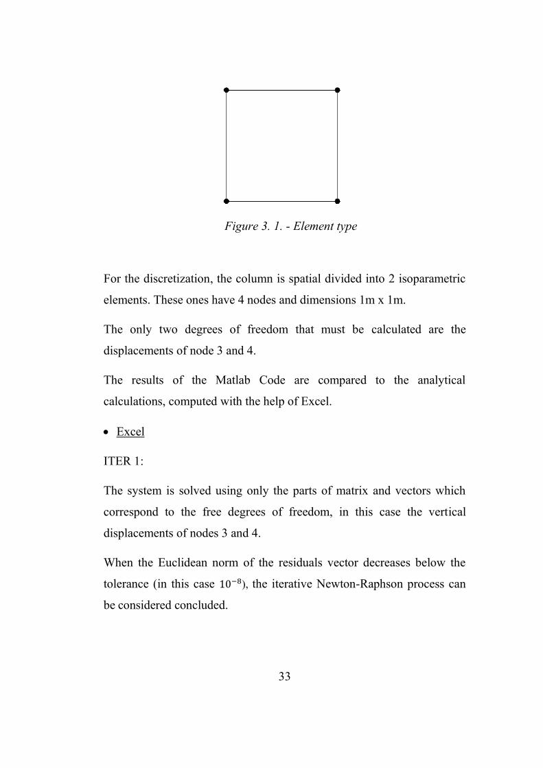
For the discretization, the column is spatial divided into 2 isoparametric
elements. These ones have 4 nodes and dimensions 1m x 1m.
The only two degrees of freedom that must be calculated are the
displacements of node 3 and 4.
The results of the Matlab Code are compared to the analytical
calculations, computed with the help of Excel.
Excel
ITER 1:
The system is solved using only the parts of matrix and vectors which
correspond to the free degrees of freedom, in this case the vertical
displacements of nodes 3 and 4.
When the Euclidean norm of the residuals vector decreases below the
tolerance (in this case 10−8), the iterative Newton-Raphson process can
be considered concluded.
Figure 3. 1. - Element type

34
Table 3. 1. - Iter one. Analytical results.
ITER 2:
Table 3. 2. - Iter two. Analytical results.
Free DOFs Residuals
20000,1685 -0,1685 Δv3 10
0,0000 20000,1685 Δv4 10
Residuals Δv
5,00E-05 4,21E-10 10 0,0005
0 5,00E-05 10 0,000499996
v new Euclidean norm
v3 0,0005 14,14213562
v4 0,000499996
=
Stiffness Matrix of the free DOFs
Inverse of the Stiffness Matrix
=
Free DOFs Residuals
20000,1685 -0,1685 Δv3 -8,88E-16
0,0000 20000,1685 Δv4 8,43E-05
Residuals Δv
5,00E-05 4,21E-10 10 3,55E-14
0 5,00E-05 10 4,21E-09
v new Euclidean norm
v3 0,0005 8,43E-05
v4 0,0005
=
Stiffness Matrix of the free DOFs
Inverse of the Stiffness Matrix
=

35
ITER 3:
Table 3. 3. - Iter three. Analytical results.
In three iterations the system of equations converges and the norm goes
to zero. The result is what we expected to have.
Matlab Code
Free DOFs Residuals
20000,1685 -0,1685 Δv3 8,88E-16
0,0000 20000,1685 Δv4 7,11E-15
Residuals Δv
5,00E-05 4,21E-10 8,88E-16 4,44E-20
0 5,00E-05 7,11E-15 3,55E-19
v new Euclidean norm
v3 0,0005 7,16E-15
v4 0,0005
=
Stiffness Matrix of the free DOFs
Inverse of the Stiffness Matrix
=
DOF VALUE U1 0 V1 0 P1 0 U2 0 V2 0 P2 0 U3 0 V3 5*10^-4 P3 0 U4 0 V4 5*10^-4 P4 0 U5 0 V5 1*10^-3 P5 0 U6 0 V6 1*10^-3 P6 0
Table 3. 4. - Numerical results.
Figure 3. 2. - Spectrum of displacements

36
The vector with all the degrees of freedom and the diagram of
displacements along the two-element column show how the code
perfectly fits to the analytical solution.
This output is obtained after to iterations only:
After the second iteration in fact the Euclidian norm is decreased below
the tolerance.
In this particular comparison a geometrical model formed by two
elements only is created, to have a more simple system and make the
analytical computations simpler. Analogue results are however reached
also considering a different mesh formed by more elements.
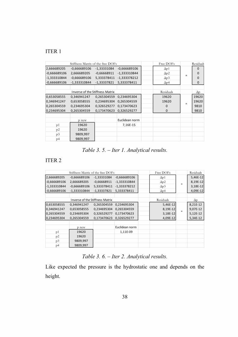
3.2.2. Step 2
The aim of this second sub-case is checking the pressures alone. In other
words we want to control the element 𝐾22 of the global stiffness matrix.
For this reason the parameter 𝛼, which links displacements and
pressures, is maintained equal to zero.
Even the geometry is maintained the same of the previous example. The
changes are in terms of applied load. There are no more displacements
applied on the top, but the gravity 𝑔 = 9,81 𝑚/𝑠2 is the only external
load. It will not be applied on the nodes, but it becomes part of the

37
equations themselves, in particular of the term 𝑓𝑝 in correspondence of
the vector; previously named 𝑏.
The boundary conditions infect the pressure on the top (nodes 5 and 6)
and are fixed to zero.
What we expect at the end of this simulation, is an hydrostatic
distribution of pressures along the entire high of the column.
Excel
𝜌𝑠 = 2000𝑘𝑔
𝑚3
𝜌𝑤 = 1000 𝑘𝑔/𝑚3
𝐸 = 2 ∙ 1010𝑃𝑎
𝑔 = 9,81 𝑚/𝑠2
Figure 3. 3. - Representation of geometry and list of material parameters.
Figure 3. 4. - Representation of the geometry and list of material parameters
38
ITER 1
Table 3. 5. – Iter 1. Analytical results.
ITER 2
Table 3. 6. – Iter 2. Analytical results.
Like expected the pressure is the hydrostatic one and depends on the
height.
Free DOFs Residuals
2,666689205 -0,666689106 -1,33331084 -0,666689106 Δp1 0
-0,666689106 2,666689205 -0,66668911 -1,333310844 Δp2 0
-1,333310844 -0,666689106 5,333378411 -1,333378212 Δp3 0
-0,666689106 -1,333310844 -1,33337821 5,333378411 Δp4 0
Residuals Δp
0,653058555 0,346941247 0,265304559 0,234695304 19620 19620
0,346941247 0,653058555 0,234695304 0,265304559 19620 19620
0,265304559 0,234695304 0,326529277 0,173470623 0 9810
0,234695304 0,265304559 0,173470623 0,326529277 0 9810
p new Euclidean norm
p1 19620 7,16E-15
p2 19620
p3 9809,997
p4 9809,997
=
Inverse of the Stiffness Matrix
=
Stiffness Matrix of the free DOFs
Free DOFs Residuals
2,666689205 -0,666689106 -1,33331084 -0,666689106 Δp1 5,46E-12
-0,666689106 2,666689205 -0,66668911 -1,333310844 Δp2 8,19E-12
-1,333310844 -0,666689106 5,333378411 -1,333378212 Δp3 3,18E-12
-0,666689106 -1,333310844 -1,33337821 5,333378411 Δp4 4,09E-12
Residuals Δp
0,653058555 0,346941247 0,265304559 0,234695304 5,46E-12 8,21E-12
0,346941247 0,653058555 0,234695304 0,265304559 8,19E-12 9,07E-12
0,265304559 0,234695304 0,326529277 0,173470623 3,18E-12 5,12E-12
0,234695304 0,265304559 0,173470623 0,326529277 4,09E-12 5,34E-12
p new Euclidean norm
p1 19620 1,11E-09
p2 19620
p3 9809,997
p4 9809,997
=
Inverse of the Stiffness Matrix
=
Stiffness Matrix of the free DOFs

39
In two iterations the system of equations converges and the norm goes to
zero.
Matlab Code
Figure 3. 4. – Spectrum of pressures.
The results showed, both in the table and both in the colored diagram,
are right and the same of the analytical calculations.
The precise solution is reached in two iterations:
3.2.3. Step 3
After the validation of the program respectively in the decoupled case of
displacements alone or pressure alone, the coupled case is considered.
Fixed the parameter 𝛼 = 0, the 𝐾21and 𝐾21elements of the stiffness
matrix begin to be significant and assume values different from zero.
DOF VALUE P1 0 P2 0 P3 9810 P4 9810 P5 19620 P6 19620
Table 3. 7. – Numerical results.

40
The case of a column, 10m high, composed by ten square elements 1x1
is considered. The only contribute of the external forces is due to the
gravity.
First, the analytical solution has to be calculated, in order to have a basis
for comparison.
The analysed system and the material parameters used in this example
are summarized in Figure 3.6..
𝜌𝑠 = 2000𝑘𝑔
𝑚3
𝜌𝑤 = 1000 𝑘𝑔/𝑚3
𝐸 = 2 ∙ 1010𝑃𝑎
𝑔 = 9,81 𝑚/𝑠2
Figure 3. 5. – Representation of geometry and list of the material parameters.

41
The width of the elements is the unit, in order to assume the plane stress
state.
As already said, the only external force is the weight force of the grains
themselves. The effective stress 𝜎(𝑧)′ is therefore calculated as:
𝜎′(𝑧) = 𝛾′𝑧 (3.1)
where 𝛾′is effective part of the specific weight 𝛾 of the global material.
It can be in fact written as:
𝛾′ = 𝛾 − 𝛾𝑤 (3.2)
where 𝛾𝑤is the water specific weight.
The terms above can be rewritten using respectively the mixture density
𝜌𝑚𝑖𝑥 and the water density 𝜌𝑤:
𝛾 = 𝜌𝑚𝑖𝑥𝑔 = (1 − 𝑛)𝜌𝑠 + 𝑛𝜌𝑤 (3.3)
𝛾𝑤 = 𝜌𝑤𝑔 (3.4)
with 𝜌𝑠 density of the solid skeleton.
The effective part of the specific weight is therefore explicated as:
𝛾′ = [(1 − 𝑛)𝜌𝑠 + (𝑛 − 1)𝜌𝑤]𝑔 = 6891,52 𝑁/𝑚2 (3.5)
It is now necessary to find the law for the strain 𝜀(𝑧) and to integrate it in
order to obtain the relative displacements ∆𝐿.
The strain law can be deduced by the stress one:
𝜀(𝑧) =𝜎(𝑧)
𝐸 (3.6)

42
and the stretching is therefore:
∆𝐿(𝑧) = ∫ 𝜀 𝑑𝑧𝑧
0= ∫
𝛾′𝑧
𝐸𝑑𝑧 =
𝛾′
𝐸∫ 𝑧
𝑧
0𝑑𝑧 =
𝛾′
𝐸
𝑧2
𝑑
𝑧
0 (3.7)
We can now calculate for example the hugest stretching, that is the
incremental displacement of the superior element (nodes 21-22), which
is:
∆𝐿(𝑧 = 10) =𝛾′
𝐸
ℎ2
2= 0,0000072288125 𝑚 (3.8)
The next step is therefore the comparison between this result and the
numerical output of Matlab Code.
The gait of pressure and displacement is reported in the following
images:
Figure 3. 6. Spectrum of pressures
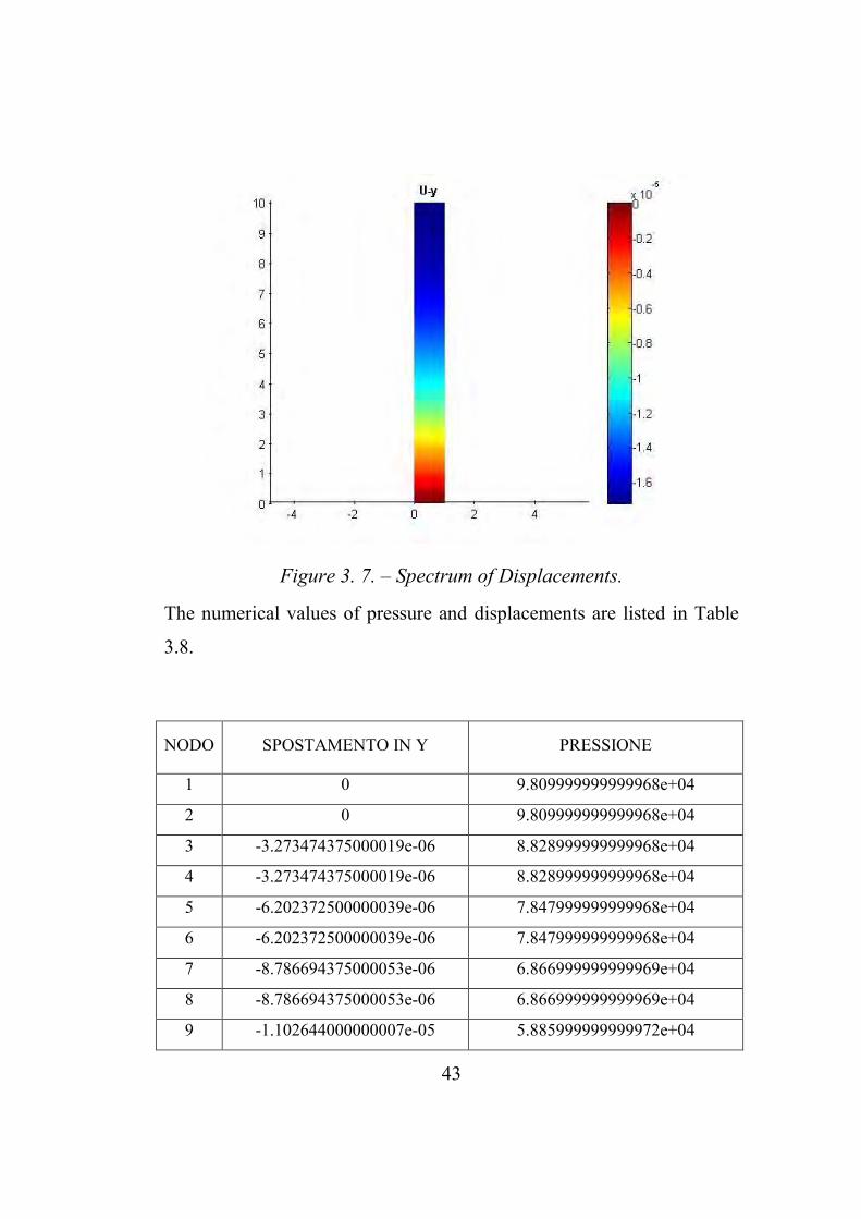
43
Figure 3. 7. – Spectrum of Displacements.
The numerical values of pressure and displacements are listed in Table
3.8.
NODO SPOSTAMENTO IN Y PRESSIONE
1 0 9.809999999999968e+04
2 0 9.809999999999968e+04
3 -3.273474375000019e-06 8.828999999999968e+04
4 -3.273474375000019e-06 8.828999999999968e+04
5 -6.202372500000039e-06 7.847999999999968e+04
6 -6.202372500000039e-06 7.847999999999968e+04
7 -8.786694375000053e-06 6.866999999999969e+04
8 -8.786694375000053e-06 6.866999999999969e+04
9 -1.102644000000007e-05 5.885999999999972e+04

44
10 -1.102644000000007e-05 5.885999999999972e+04
11 -1.292160937500009e-05 4.904999999999976e+04
12 -1.292160937500009e-05 4.904999999999976e+04
13 -1.447220250000010e-05 3.923999999999981e+04
14 -1.447220250000010e-05 3.923999999999981e+04
15 -1.567821937500010e-05 2.942999999999986e+04
16 -1.567821937500010e-05 2.942999999999986e+04
17 -1.653966000000011e-05 1.961999999999991e+04
18 -1.653966000000011e-05 1.961999999999991e+04
19 -1.705652437500011e-05 9.809999999999953e+03
20 -1.705652437500011e-05 9.809999999999953e+03
21 -1.722881250000012e-05 0
22 -1.722881250000012e-05 0
Table 3. 8. – Numerical results.
As expected, pressures keep their hydrostatic behaviour.
The displacements results are validated too. Their values in
correspondence of nodes 21 and 22 (highlighted in bold in Table 3.8.)
are in fact the same calculated in (3.8) with the analytical method.
3.2.4. Step 4
This step contains the validation of the model in the same load and
geometrical conditions of “step 3”, comparing the results at each time
step with the program Comes-GeoPZ. The aim is checking the right
transmission of the load in time.
The material parameters in this example are the following:

45
𝜌𝑤 = 1000 𝑘𝑔/𝑚3 water density
𝜌𝑠 = 2000 𝑘𝑔/𝑚3 grains density
𝐸 = 30 ∙ 106𝑃𝑎 Young modulus of the soil
𝜈 = 0 Posson ratio of the soil
𝐾𝑠 = 6.78 ∙ 109𝑃𝑎 bulk modulus of the grains
𝐾𝑤𝑎 = 0.2 ∙ 109 𝑃𝑎 bulk modulus of the water
𝑘𝑤𝑖 = 4.5 ∙ 10−13𝑚2 intrinsic permeability
𝜇𝑤 = 0.001𝑘𝑔
𝑚∙𝑠 water viscosity
The analysis is carried on using steps of time of 100s.
Previously, the program Comes-GeoPZ is run. Noticed that the complete
consolidation is reached after 238 steps, our steps are fixed at the number
of 250.
Next, the results after step 1, 50, 150 and 250 are copied out.
We compare the results of the two programs in terms of maximum
pressure, measured at the bottom of the column.
In Comes-GeoPz the water pressure 𝑝𝑐 is calculated, while with the
Matlab Code the output is the water pressure. The modulus is the same,
only the sign obviously changes.

46
Time step 1 t=100 s
Comes
Figure 3. 8. – Time step 1. Numerical results with Comes.
Matlab
Figure 3. 9. Time step 1. Numerical results for pressure with Matlab
code.

47
Time step 50 t=5000s
Comes
Figure 3. 10. Time step 50. Numerical results with Comes.
Matlab
Figure 3.11. – Time step 50. Numerical results for pressure with Matlab code.

48
Time step150 t=15000s
Comes
Figure 3. 12. – Time step 150. Numerical results with Comes.
Matlab
Figure 3. 13. – Time step 150. Numerical results for pressure with Matlab code.

49
Time step250 t=25000s
Comes
Figure 3. 14. – Time step 250. Numerical results with Comes.
Matlab
Figure 3. 15. – Time step 250. Numerical results for pressure with Matlab code.

50
The two models are comparable. We can easily notice that the process of
consolidation is not really finished at step 250. The decimal places
neglected by Comes are not null yet.
Going on with the time steps, the solution slowly tends to the precise
expected value of 98100 Pa.
The results in terms of pressure and displacements at the 400th time step
are therefore given (Figure 3.17).
Figure 3. 16 – Time step 400. Numerical results with Matlab code.

51
3.2.5. Step 5
In this last example with a fully saturated condition of flow, the load
conditions and the initial conditions change, while the geometry and the
spatial constraints remain the same.
At time 𝑡 = 0, the process of consolidation is considered finished. As
initial conditions, the hydrostatic trend of pressure and the deformation
field at the end of the consolidation process are assumed. In other words
the results of previous Step 4 can be considered the start of this new
case.
As for the applied load, a mechanical vertical load of 10.000 Pa is acting
on the top of the ten elements-column.
The system is represented in Figure (3.18).
Figure 3. 18. – Representation of the geometry.

52
The development of the water pressure we expect to find, is the
following one, described by Figure (3.19).
Figure 3. 19. – Representation of the geometry.
Starting from an hydrostatic configuration (phase 0), water pressures
should initially adsorb the whole entity of the applied load (phase 1), and
then pass it on to the solid skeleton, returning therefore to the initial
condition (phase 2).
In this particular case, in order to fix a boundary condition for the water
pressure, this last one is fixed zero on the nodes 21 and 22. This creates a
discrepancy in the trend in correspondence of the superior part of the
column between Figure 3.19 and the numerical implementation.
The applied load is inserted into the code, by adding it to the residual
term of the first momentum equilibrium equation.

53
It needs his own loop of integration between node 21 and 22, using the
interpolation functions of a two-node element.
Next, the results at some significant time-steps are reported. Even in this
case, they are compared to the outputs of an existent model for the
consolidation in Comes.
Time step1 t=100s
This is the initial step, in which the water takes all the load.
The water pressure value at nodes 1 and 2 must be the sum between the
initial hydrostatic pressure and the applied tension:
𝑝𝑤(𝑛𝑜𝑑𝑒 1) = 98100 + 10000 = 108100𝑃𝑎 = 1,081 ∙ 105𝑃𝑎
Indeed, both Comes and Matlab give this result, as shown in Figure
(3.20-3.21).
Figure 3. 20. – Time step 1. Numerical results for pressure with Matlab code.

54
Figure 3. 21. – Time step 1. Numerical results for pressure with Comes.
Time step50 t=5000s
Matlab results are firstly shown. Therefore the comparison between it
and Comes is represented in a graph.
Figure 3. 22. – Time step 50. Numerical results with Matlab code.

55
Figure 3. 23. – Time step 50. Comparison Matlab/Comes for pressures.
Figure 3. 24. – Time step 50. Comparison Matlab/Comes for displacements.

56
Time step100 t=10000s
Matlab results are firstly shown. Therefore the comparison between it
and Comes is represented in a graph.
Figure 3. 25. – Time step 100. Numerical results with Matlab code.

57
Figure 3. 26. – Time step 100. Comparison Matlab/Comes for pressures.
Figure 3. 27. – Time step 100. Comparison Matlab/Comes for
displacements.

58
Time step250 t=25000s
Matlab results are firstly shown. Therefore the comparison between it
and Comes is represented in a graph.
Figure 3. 28. – Time step 250. Numerical results with Matlab code.

59
Figure 3. 29. – Time step 250. Comparison Matlab/Comes for pressure.
Figure 3. 30. – Time step 250. Comparison Matlab/Comes for displacements.

60
Conclusions
After 250 time step, that is after 25000 seconds, the load is completely
transmitted from the water to the solid skeleton.
Water pressures settle themselves again in their hydrostatic trend, while
the displacements reach the maximum value on the top of -1,235 cm.
Purified of the initial displacement due to the process of consolidation
(-0.957 cm), the maximum displacement caused by the applied load has
a value of -1.139 cm.
The code can be considered validated in fully saturated conditions, as the
comparison with Comes at different time steps proves.
3.3. Partially Saturated conditions
3.3.1. Explanation of the benchmark
In this last test, the aim was the validation of the model in condition of
partially saturated soil.
It is difficult to choose appropriate tests to validate the model developed
in the previous sections and its implementation in the computer code.
Indeed there are no analytical solution for this type of coupled problems,
where deformations of the solid skeleton are studied with saturated-
unsaturated flow of mass transfer. There are also very few documented
laboratory experiments.
One of these is the experiment conducted by Liakopoulos on the
isothermal drainage of water from a vertical column of water saturated

61
sand. The column is one meter high, subdivided into ten quadrilateral
elements of 0.1 x 0.1 meters. All the nodes of the column are fixed along
the horizontal direction. The base of the column is also fixed for the
vertical displacements.
The column was packed by Del Monte sand and instrumented to measure
the moisture tension at several points along the column. Before starting
the experiment (t < 0) water was continuously added from the 28 The
Erwin Stein Award top and was allowed to drain freely at the bottom
through a filter. The flow was carefully regulated until the tensiometers
read zero pore pressure. At t = 0 the water supply was ceased and the
tensiometers reading were recorded.
Only the porosity and the hydraulic properties of Del Monte sand were
measured by an independent set of experiments. Material parameters and
the experimental constitutive laws for 𝑆𝑤(𝑝𝑐) and 𝑘𝑟𝑤(𝑝𝑐) used in the
computation are listed in (Table 3.9.).
PARAMETER VALUE
Porosity 𝑛 = 0.2975
Isotropic permeability 𝑘 = 4.3 ∙ 10−6𝑚/𝑠
Solid grain density 𝜌𝑠 = 2000 𝑘𝑔/𝑚3
Water density 𝜌𝑤 = 1000 𝑘𝑔/𝑚3
Gravity acceleration 𝑔 = 9.806 𝑚/𝑠
Water saturation 𝑆𝑤 = 1 − 1.9722 ∙ 1011𝑝𝑐2.4279
Relative permeability for water 𝑘𝑟𝑤 = 1 − 2.207(1 − 𝑆𝑤)1.0121
Solid bulk modulus 𝐾 = 2166.77 𝑘𝑁/𝑚3
Table 3. 9. – Parameters.

62
3.3.2. Implementation: results and validation
Liakopoulus’ column is made of consolidated sand. As initial condition
for modelling, the pressures and the dispalcements obtained after Step 4
(consolidation) are imposed. Water pressure at the bottom is fixed zero,
to simulate the dreinage of water.
The simulation is divided into time steps of 𝑡 = 10𝑠.
The compairson with the Liakopoulus test implemented with Comes are
done at different time steps: 5, 30, 60 and 120 minutes.
The results in terms of water pressure, displacement and saturation
degree are shown below.
Water pressure
A compairson between Matlab code and Comes at each time step will be
described in the next graphs.
After them, another diagram will show the evolution of water pressure
during the time.

63
Figure 3. 31. – Time step 30. Comparison Matlab/Comes for pressure.
Figure 3. 32. – Time step 180. Comparison Matlab/Comes for pressure.

64
Figure 3. 33. – Time step 360. Comparison Matlab/Comes for pressure.
Figure 3. 34. – Time step 720. Comparison Matlab/Comes for pressure.
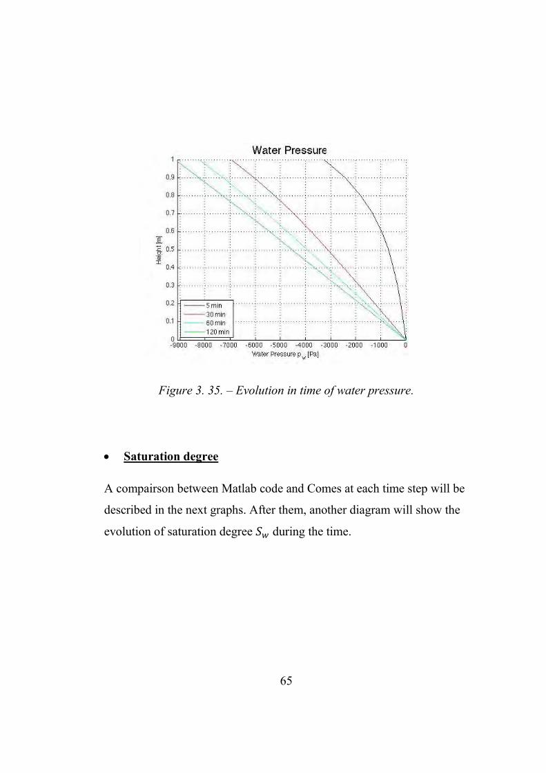
65
Figure 3. 35. – Evolution in time of water pressure.
Saturation degree
A compairson between Matlab code and Comes at each time step will be
described in the next graphs. After them, another diagram will show the
evolution of saturation degree 𝑆𝑤 during the time.

66
Figure 3. 36. – Time step 30. Comparison Matlab/Comes for Sw.
Figure 3. 37. – Time step 180. Comparison Matlab/Comes for Sw.

67
Figure 3. 38. – Time step 360. Comparison Matlab/Comes for Sw.
Figure 3. 39. – Time step 720. Comparison Matlab/Comes for Sw.

68
Figure 3. 40. – Evolution in time of saturation degree.
Displacements
A compairson between Matlab code and Comes at each time step will be
described in the next graphs. After them, another diagram will show the
evolution of displacments during the time.
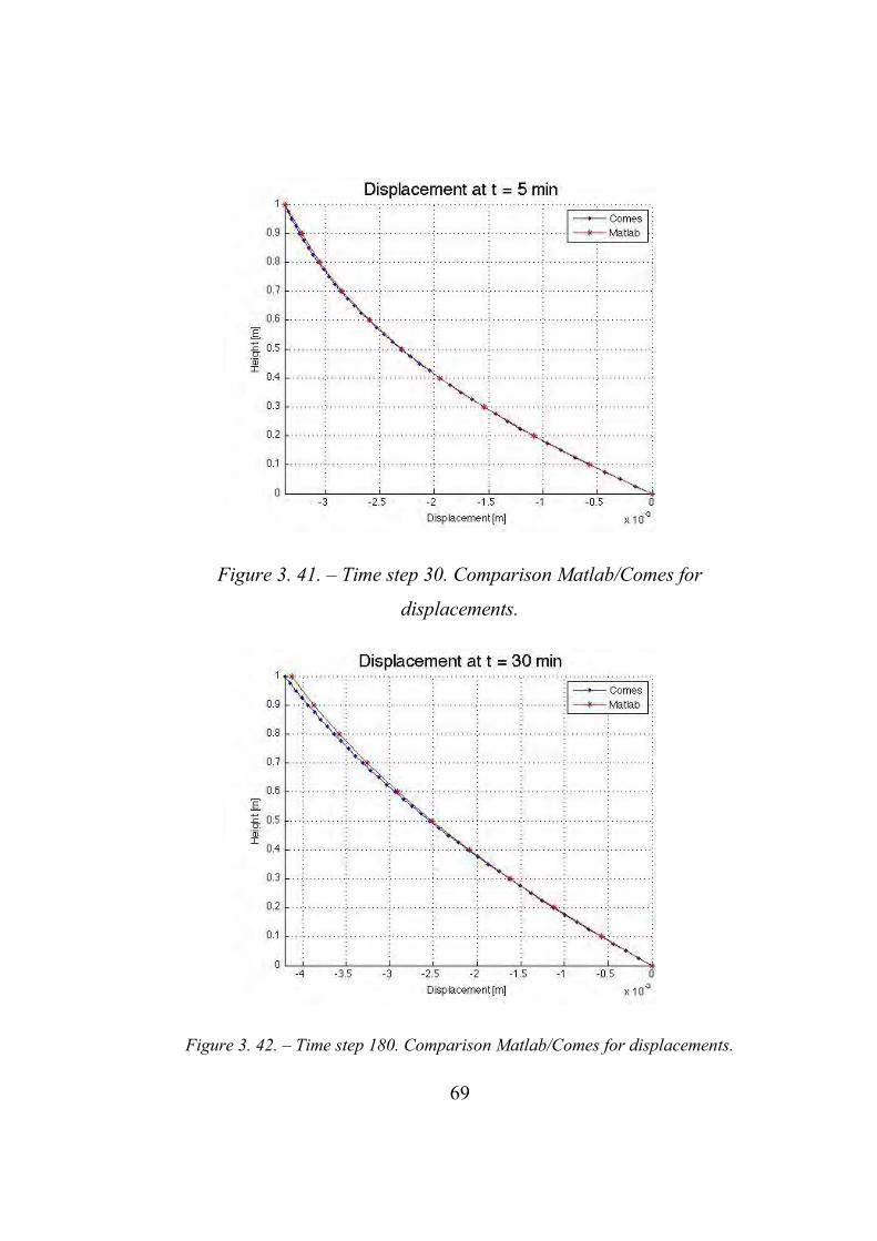
69
Figure 3. 41. – Time step 30. Comparison Matlab/Comes for
displacements.
Figure 3. 42. – Time step 180. Comparison Matlab/Comes for displacements.
70
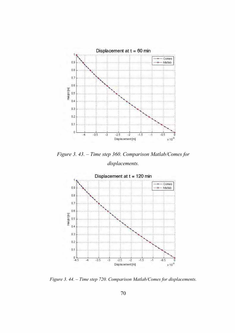
Figure 3. 43. – Time step 360. Comparison Matlab/Comes for
displacements.
Figure 3. 44. – Time step 720. Comparison Matlab/Comes for displacements.

71
Figure 3. 45. – Evolution in time of displacements.
3.3.3. Conclusions
After 2 hours the process is almost concluded. The water pressure on the
top should in fact reach the value of 𝑝𝑤 = −9810 𝑃𝑎 , linearly
decreasing his absolute value until reaching the null pressure at the
bottom.
The model implemented in Matlab can be considered validated. It fits in
fact with the Comes results.

72
Chapter 4 - The phase-field description of
dynamic brittle fracture
4.1. Introduction to phase field As experimental tests are expensive and time consuming, they cannot be
carried out at all stages of a design process in an efficient and
economical way. Thus, conclusions drawn from numerical simulations
often play a crucial role in design decisions. This happens even in the
case of the study of material fractures.
As a consequence, lots of research effort is put into the development of
reliable fracture models and the numerical implementation thereof. The
key objective of these fracture models is the prediction of the fracture
evolution in a given loading situation. On the one hand, this requires
criteria for the onset of crack extension of pre-existing cracks and for the
nucleation of new cracks in originally undamaged material. On the other
hand, the geometry of the crack path, including possible kinking of a
crack or bifurcation into several crack branches, needs to be predicted. In
dynamic fracture mechanics, also the velocity of crack propagation is an
issue.
The theoretical foundations of the contemporary theory of brittle fracture
were laid in the works of Griffith [1921] and Irwin [1957]. Griffith was
the first to link the energy necessary for the breaking of atomic bonds to
an energy density of crack surfaces. As a consequence, he formulated an
energetic fracture criterion, where crack propagation results from the

73
competition of elastic energy stored in the solid and surface energy
needed to create new fracture surfaces. The actual breakthrough of this
new concept was achieved through the works of Irwin. Besides a
refinement of the surface energy density proposed by Griffith, he
characterized the loading of a crack in terms of singular stresses at the
crack tip, and proved the equivalence of his method and Griffith’s
energetic approach. This link allows to evaluate cracks using the tools of
classical continuum mechanics and opened the door to practical
applications of the new concepts and to further research in the field of
theoretical fracture mechanics.
Besides the development of physically sound and appropriate models of
crack propagation, numerical instruments are needed to describe the
elastic deformations of complex structures, which generally cannot be
obtained analytically. To this end, particularly the finite element method
(FEM) is widely used in industrial applications. The essential
characteristic of this method is the discretization of a continuous
structure into a set of sub-domains referred to as elements with a certain
number of element nodes. The partial differential equations for the
unknown field variables are then recast into a finite dimensional set of
equations for the discrete nodal values. In between the element nodes,
the unknown field variables are usually approximated by means of
continuous shape functions. Consequently, finite elements do not cope
well with field discontinuities. This challenges their application in the
context of fracture mechanics, because at a crack the displacement field
may suffer jump discontinuities.

74
In this regard, a conceptually different modeling approach to fracture has
gained importance in recent years. The so called phase field method
bases on concepts elaborated by Ginzburg and Landau [1959] and was
originally introduced by Collins and Levine [1985] and Caginalp and
Fife [1986] in order to model solidification processes. The general idea
of this modeling approach is the incorporation of an additional
continuous field variable – the phase field order parameter – whose value
describes the condition of the system. At interfaces between different
material phases, the order parameter interpolates smoothly between the
values assigned to the different phases, avoiding discontinuous jumps.
The width of the diffuse transition zone between different material
phases is controlled by a model inherent length scale. If this length scale
becomes infinitesimal small, the underlying sharp interface model is
recovered. In a phase field model, the motion of the interfaces is given
implicitly by the solution of a partial differential equation for the order
parameter. This so called evolution equation is coupled to the elastic
field equations in order to model the mutual interaction between the
phase state and the elastic properties of the material. This coupling also
has the effect that the boundary conditions at phase interfaces are
automatically satisfied, thus avoiding an explicit treatment thereof. This
property is also very advantageous concerning numerical simulations and
significantly facilitates the study of structures with more complex
interface geometries. Thus, the phase field method is a very powerful
numerical tool to solve moving boundary problems.

75
4.2. General remarks In this thesis a continuum approach to brittle fracture is used. This means
that the material is treated as a continuum, and fracture is predicted on
the basis of an analysis of macroscopic quantities stress, energy and
strain. from this point of view, a crack is a cut in the body at the scale of
the structure. The dimension of a crack is considered to be one
dimension lower than the geometrical dimension of the surrounding
material.
A crack is a line and its end point is called crack tip, in two-dimensional
media. In three-dimensional media, a crack forms a surface ending at the
crack front. The opposite boundaries of a crack are called crack faces.
These ones are considered to be traction free in most applications.
The loading of a crack can be described with three independent
components according to the figure. Mode one is a symmetric crack
opening orthogonal to the local fracture surface. It is the most important
case for practical application. In mode two, the crack surface slide
relatively to each other in the plane of the crack and perpendicular to the
crack front, causing shear stresses. In mode three, crack surfaces separate
in the plane of the crack, but parallel to the crack front.

76
Figure 4. 1. Crack opening modes.
4.3. Model assumption in LEFM The complex processes of bond breaking in front of the crack front or
crack tip are not explicitly described by continuum approaches to
fracture. Therefore, the process zone, in which these events take place,
must be negligibly small compared to all macroscopic dimensions of the
investigated structure. This assumption holds true for many brittle
materials and is a typical feature of metals.
In reality, the material will deform inelastically in the so called yielding
zone around the crack tip. Thus, linear theory is applicable, if the
yielding zone is limited to a very small area around the crack. Which
holds true for many brittle but not for ductile materials.
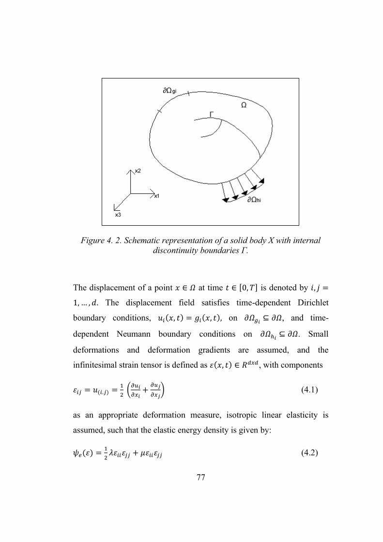
4.4. Griffith’s theory of brittle fracture An arbitrary body 𝛺 ⊂ 𝑅𝑑 (with 𝑑 ∈ 1, ,2,3) with external boundary 𝜕𝛺
and internal discontinuity boundary Γ is considered.
77
Figure 4. 2. Schematic representation of a solid body X with internal discontinuity boundaries Γ.
The displacement of a point 𝑥 ∈ 𝛺 at time 𝑡 ∈ [0, 𝑇] is denoted by 𝑖, 𝑗 =
1,… , 𝑑. The displacement field satisfies time-dependent Dirichlet
boundary conditions, 𝑢𝑖(𝑥, 𝑡) = 𝑔𝑖(𝑥, 𝑡), on 𝜕𝛺𝑔𝑖⊆ 𝜕𝛺, and time-
dependent Neumann boundary conditions on 𝜕𝛺ℎ𝑖⊆ 𝜕𝛺. Small
deformations and deformation gradients are assumed, and the
infinitesimal strain tensor is defined as 𝜀(𝑥, 𝑡) ∈ 𝑅𝑑𝑥𝑑, with components
𝜀𝑖𝑗 = 𝑢(𝑖.𝑗) =1
2 (
𝜕𝑢𝑖
𝜕𝑥𝑖+
𝜕𝑢𝑗
𝜕𝑥𝑗) (4.1)
as an appropriate deformation measure, isotropic linear elasticity is
assumed, such that the elastic energy density is given by:
𝜓𝑒(𝜀) =1
2𝜆𝜀𝑖𝑖𝜀𝑗𝑗 + 𝜇𝜀𝑖𝑖𝜀𝑗𝑗 (4.2)
78
with 𝜆 and 𝜇 the Lamé constants. The Einstein summation convention is
used on repeated indices.
The evolving internal discontinuity boundary, Γ(t), represent a set of
discrete cracks. In according with Griffith’s theory of brittle fracture, the
energy required to create a unit area of fracture surface is equal to the
critical fracture energy density 𝒢𝑐. The total potential energy of the body,
𝜓𝑝𝑜𝑡, being the sum of the elastic energy and the fracture energy, is the
given by
𝜓𝑝𝑜𝑡(𝑢, 𝛤) = ∫ 𝜓𝑒(∇𝑠𝑢)𝑑𝑥
𝛺+ ∫ 𝒢𝑐𝑑𝑥
𝛤 (4.3)
the symmetric gradient operator, ∇𝑠: 𝑢 → 𝜀, is defined as a mapping from
the displacement field to the strain field. Since brittle fracture is
assumed, the fracture energy contribution is merely the critical fracture
energy density integrated over the fracture surface. In the case of small
deformations, irreversibility of the fracture process dictates that 𝛤(𝑡) ⊆
𝛤(𝑡 + ∆𝑡) for all ∆𝑡 > 0. Hence, translation of cracks through the domain
is prohibited, but cracks can extend, branch and merge.
The kinetic energy of the body Ω is given by:
𝜓𝑘𝑖𝑛() =1
2∫ 𝜌𝑖𝑖𝑑𝑥𝛺
(4.4)
with =𝜕𝑢
𝜕𝑡 and 𝜌 the mass density of the material. Combined with the
potential energy this renders the Lagrangian for the discrete fracture
problem as:

79
𝐿(𝑢, , 𝛤) = 𝜓𝑘𝑖𝑛() − 𝜓𝑝𝑜𝑡 = ∫ [1
2𝜌𝑖𝑖 − 𝜓𝑒(∇
𝑠𝑢)] 𝑑𝑥𝛺
− ∫ 𝒢𝑐𝑑𝑥𝛤
(4.5)
The Euler-Lagrange equations of this functional determine the motion of
the body. From a numerical standpoint, tracking the evolving
discontinuity boundary, Γ, often requires complex and costly
computations. This is particularly so when interactions between multiple
cracks, or complex shaped cracks in three dimensions are considered.
4.5. Phase-field approximation
4.4.1. Phase field theory
In order to circumvent the problems associated with numerically tracking
the propagating discontinuity representing a crack, the fracture surface,
Γ, is approximated by a phase-field, 𝑠(𝑥, 𝑡) ∈ [0,1]. The value of this
phase field is equal to 1 away from the crack and is equal to 0 inside the
crack. As in Bourdin the fracture energy is approximated by:
∫ 𝒢𝑐𝑑𝑥𝛤
≈ ∫ 𝒢𝑐 [(𝑠−1)2
4𝑙0+ 𝑙0
𝜕𝑠
𝜕𝑥𝑖
𝜕𝑠
𝜕𝑥𝑖] 𝑑𝑥
𝛺 (4.6)
where 𝑙0 ∈ ℝ+is a model parameter that controls the width of the smooth
approximation of the crack. From Eq (4.6) it is clear that a crack is
represented by regions where the phase field goes to zero. As elaborated
by Bourdin n the limit of the length scale 𝑙0 going to zero, the phase field
approximation converges to the discrete fracture surface.
To model the loss of material stiffness in the failure zone, it is followed
Miehe and the elastic energy is defined as:

80
𝜓𝑒(𝜀, 𝑠) = [(1 − 𝑘)𝑠2 + 𝑘]𝜓𝑒+(𝜀) + 𝜓𝑒
−(𝜀) (4.7)
where 𝜓𝑒+(𝜀) and 𝜓𝑒
−(𝜀) are the strain energies computed from the
positive and negative components of the strain tensor, respectively,
defined through a spectral decomposition of strain. Let:
𝜀 = 𝑃𝛬𝑃𝑇 (4.8)
where P consists of the orthonormal eigenvectors of 𝜀 and 𝛬 =
𝑑𝑖𝑎𝑔(𝜆1, 𝜆2, 𝜆3) is a diagonal l matrix of principal strains. Defining:
𝜀+ = 𝑃𝛬+𝑃𝑇 (4.9)
𝜀− = 𝑃𝛬−𝑃𝑇 (4.10)
where:
𝛬+ = 𝑑𝑖𝑎𝑔(⟨𝜆1⟩, ⟨𝜆2⟩, ⟨𝜆3⟩) (4.11)
𝛬− = 𝛬 − 𝛬+ (4.12)
and
⟨𝑥⟩ = 𝑥 𝑥 > 00 𝑥 ≤ 0
(4.13)
Then:
𝜓𝑒+(𝜀) =
1
2𝜆⟨𝑡𝑟𝜀⟩2 + 𝜇𝑡𝑟[(𝜀+)2] (4.14)
and
𝜓𝑒−(𝜀) =
1
2𝜆(𝑡𝑟𝜀 + ⟨𝑡𝑟𝜀⟩)2 + 𝜇𝑡𝑟[(𝜀 − 𝜀+)2]. (4.15)

81
the intent of the model is to maintain resistance in compression and, in
particular, during crack closure. All calculations in this model set 𝑘 = 0
because its inclusion is unnecessary.
Substitution of the phase field approximations for the fracture energy
(4.6) and the elastic energy density (4.7) into Lagrange energy functional
(4.5) yields:
𝐿(𝑢, , 𝛤) = ∫ (1
2𝜌𝑖𝑖 − [(1 − 𝑘)𝑠2 + 𝑘]𝜓𝑒
+(∇𝑠𝑢) − 𝜓𝑒−(∇𝑠𝑢)) 𝑑𝑥
𝛺−
∫ 𝒢𝑐 [(𝑠−1)2
4𝑙0+ 𝑙0
𝜕𝑠
𝜕𝑥𝑖
𝜕𝑠
𝜕𝑥𝑖] 𝑑𝑥
𝛺 (4.17)
In order to conserve mass kinetic energy term is unaffected by the phase
field approximation. The dependence of Lagrange energy functional on
the propagating discontinuity boundary id now captured by the phase
field, 𝑠(𝑥, 𝑡), which simplifies the numerical treatment of the model.
Miehe uses an additional viscosity contribution but hence this term is
omitted for brevity.
The Lagrangian is formulated in terms of the independent fields 𝑢(𝑥, 𝑡)
and 𝑠(𝑥, 𝑡), the Euler-Lagrange equations are used to arrive at the strong
form equations of motion:
𝜕𝜎𝑖𝑗
𝜕𝑥𝑗= 𝜌𝑖 𝑜𝑛 𝛺 × ]0, 𝑇[
(4𝑙0(1−𝑘)𝜓𝑒
+
𝒢𝑐+ 1) 𝑠 − 4𝑙0
2 𝜕2𝑠
𝜕𝑥𝑖2 = 1 𝑜𝑛 𝛺 × ]0, 𝑇[
(4.18)
where =𝜕2𝑢
𝜕𝑡2 and the Cauchy stress tensor 𝜎 ∈ ℝ𝑑×𝑑is defined by
𝜎𝑖𝑗 = [(1 − 𝑘)𝑠2 + 𝑘]𝜕𝜓𝑒
+
𝜕𝜀𝑖𝑗+
𝜕𝜓𝑒−
𝜕𝜀𝑖𝑗 (4.19)

82
These equations of motion can be solved to find both the displacement
field 𝑢(𝑥, 𝑡) and phase field 𝑠(𝑥, 𝑡). The irreversibility condition 𝛤(𝑡) ⊆
𝛤(𝑡 + ∆𝑡) is enforced in the strong form equations by introducing a
strain history field, ℋ, which satisfies the Kuhn-Tucker conditions for
loading and unloading:
𝜓𝑒+ − ℋ ≤ 0, ℋ ≥ 0, ℋ(𝜓𝑒
+ − ℋ) = 0 (4.20)
Substituting ℋ for 𝜓𝑒+ in (4.18) the modified strong form equations of
motion are:
𝜕𝜎𝑖𝑗
𝜕𝑥𝑗= 𝜌𝑖 𝑜𝑛 𝛺 × ]0, 𝑇[
(4𝑙0(1−𝑘)ℋ
𝒢𝑐+ 1) 𝑠 − 4𝑙0
2 𝜕2𝑠
𝜕𝑥𝑖2 = 1 𝑜𝑛 𝛺 × ]0, 𝑇[
(4.21)
The equation of motion are subject to the boundary conditions:
𝑢𝑖 = 𝑔𝑖 𝑜𝑛 𝜕𝛺𝑔𝑖× ]0, 𝑇[
𝜎𝑖𝑗𝑛𝑗 = ℎ𝑖 𝑜𝑛 𝜕𝛺ℎ𝑖× ]0, 𝑇[
𝜕𝑠
𝜕𝑥𝑖𝑛𝑖 = 0 𝑜𝑛 𝜕𝛺 × ]0, 𝑇[
(4.22)
with 𝑔𝑖(𝑥, 𝑡) and ℎ𝑖(𝑥, 𝑡) being prescribed on 𝜕𝛺𝑔𝑖 and 𝜕𝛺ℎ𝑖
,
respectively, for all 𝑡 ∈ ]0, 𝑇[, and with 𝑛(𝑥) being the outward-pointing
normal vector of the boundary.
In addition, the equations of motion (4.21) are supplemented with initial
conditions:
𝑢(𝑥, 0) = 𝑢0(𝑥) 𝑥 ∈ 𝛺
(𝑥, 0) = 𝑣0(𝑥) 𝑥 ∈ 𝛺
ℋ(𝑥, 0) = ℋ0(𝑥) 𝑥 ∈ 𝛺
(4.23)

83
for both the displacement field and the strain history field, ℋ0(𝑥), can be
used to model pre-existing cracks or geometrical features.
4.4.2. Numerical formulation
The numerical formulation of (4.21) requires a spatial and temporal
discretization. In this section the spatial discretization is formulated by
means of the Galerkin method and a monolithic implicit scheme is
introduced for the temporal discretization.
Continuous problem in the weak form
For the weak form of the problem it is defined a trial solution spaces 𝒮𝑡
for the displacement and 𝑡 for the phase field as:
𝒮𝑡 = 𝑢(𝑡) ∈ (𝐻1(𝛺))𝑑𝑢𝑖(𝑡) = 𝑔𝑖 𝑜𝑛 𝜕𝛺𝑔𝑖
(4.24)
𝑡 = 𝑠(𝑡) ∈ 𝐻1(𝛺) (4.25)
Similarly, the weighting function spaces are defined as:
𝜈 = 𝑤 ∈(𝐻1(𝛺))𝑑𝑤𝑖 = 0 𝑜𝑛 𝜕𝛺𝑔𝑖
(4.26)
𝜈 = 𝑞 ∈ 𝐻1(𝛺) (4.27)
Multiplying the equations in (4.21) by appropriate weighting functions
and applying integration by parts leads to the weak formulation:

84
𝐺𝑖𝑣𝑒𝑛 𝑔, ℎ, 𝑢0, 0, 𝑎𝑛𝑑 𝑠0 𝑓𝑖𝑛𝑑 𝑢(𝑡) ∈ 𝒮𝑡 𝑎𝑛𝑑 𝑠(𝑡) ∈ 𝑡 , 𝑡 ∈
[0, 𝑇], 𝑠𝑢𝑐ℎ 𝑡ℎ𝑎𝑡 𝑓𝑜𝑟 𝑎𝑙𝑙 𝑤 ∈ 𝜈 𝑎𝑛𝑑 𝑓𝑜𝑟 𝑎𝑙𝑙 𝑞 ∈ 𝜈
(𝜌𝑢, )𝛺 + (𝜎, ∇𝑤)𝛺 = (ℎ,𝑤)𝜕𝛺ℎ
((4𝑙0(1 − 𝑘)ℋ
𝒢𝑐
+ 1) 𝑠, 𝑞)
𝛺
+ (4𝑙02∇𝑠, ∇𝑞)𝛺 = (1, 𝑞)𝛺
(𝜌𝑢(0), 𝑤)𝛺 = (𝜌𝑢0, 𝑤)𝛺
(𝜌(0), 𝑤)𝛺 = (𝜌0, 𝑤)𝛺
(𝑠(0), 𝑞)𝛺 = (𝑠0, 𝑞)𝛺 (4.28)
where (∙,∙)𝛺 is thℒ2e inner product on Ω.
The semidiscrete Galerkin form
Following the Galerkin method, 𝒮𝑡ℎ ⊂ 𝒮𝑡 , 𝜈
ℎ ⊂ 𝜈, 𝑡ℎ ⊂ 𝑡 , and 𝜈ℎ ⊂ 𝜈 are
the usual finite dimensional approximations to the function spaces of the
weak form. The semidiscrete Galerkin form of the problem is then:
𝐺𝑖𝑣𝑒𝑛 𝑔, ℎ, 𝑢0, 0, 𝑎𝑛𝑑 𝑠0 𝑓𝑖𝑛𝑑 𝑢(𝑡) ∈ 𝒮𝑡 𝑎𝑛𝑑 𝑠(𝑡) ∈ 𝑡, 𝑡 ∈
[0, 𝑇], 𝑠𝑢𝑐ℎ 𝑡ℎ𝑎𝑡 𝑓𝑜𝑟 𝑎𝑙𝑙 𝑤 ∈ 𝜈 𝑎𝑛𝑑 𝑓𝑜𝑟 𝑎𝑙𝑙 𝑞 ∈ 𝜈
(𝜌𝑢, )𝛺 + (𝜎, ∇𝑤)𝛺 = (ℎ, 𝑤)𝜕𝛺ℎ
((4𝑙0(1 − 𝑘)ℋ
𝒢𝑐+ 1) 𝑠, 𝑞)
𝛺
+ (4𝑙02∇𝑠, ∇𝑞)𝛺 = (1, 𝑞)𝛺
(𝜌𝑢(0),𝑤)𝛺 = (𝜌𝑢0, 𝑤)𝛺
(𝜌(0), 𝑤)𝛺 = (𝜌0, 𝑤)𝛺
(𝑠(0), 𝑞)𝛺 = (𝑠0, 𝑞)𝛺 (4.29)

85
The explicit representations of 𝑢ℎ , 𝑤ℎ , 𝑠ℎ and 𝑞ℎ in terms of the basis
functions and nodal variables are:
𝑢𝑖ℎ = ∑ 𝑁𝐴(𝑥)𝑑𝑖𝐴
𝑛𝑏𝐴 (4.30)
𝑤𝑖ℎ = ∑ 𝑁𝐴(𝑥)𝑐𝑖𝐴
𝑛𝑏𝐴 (4.31)
𝑠ℎ = ∑ 𝑁𝐴(𝑥)𝛷𝐴𝑛𝑏𝐴 (4.32)
𝑞ℎ = ∑ 𝑁𝐴(𝑥)𝜒𝐴𝑛𝑏𝐴 (4.33)
where 𝑛𝑏 is the dimension of the discrete space, the 𝑁𝐴’s are the global
basis functions, 𝑖 is the special degree of freedom number, and
𝑑𝑖𝐴, 𝑐𝑖𝐴, 𝛷𝐴 and 𝜒𝐴 are control variable degree of freedom. The same set
of basis functions are used both for the finite dimensional trial solution
and weighting function spaces.
4.4.3. Time discretization and numerical implementation With this time discretization the momentum and phase field equations
are solved independently. At a given time step, the momentum equation
is solved first to get the displacements. Using the updated displacements,
the phase field equation is solved. Here it is presented an algorithm that
uses 𝛼 methods to solve the momentum equation.
Defining the residual vectors for the momentum and phase field
equations by:
𝑅𝐴,𝑖𝑢 = (ℎ,𝑁𝐴𝑒𝑖)𝜕𝛺ℎ
− (𝜌ℎ , 𝑁𝐴𝑒𝑖)𝛺 − (𝜎𝑗𝑘 , 𝐵𝐴𝑖𝑗𝑘
)𝛺
(4.34)
𝑅𝐴𝑠 = (1,𝑁𝐴)𝛺 − ((
4𝑙0(1−𝑘)ℋ
𝒢𝑐+ 1) 𝑠ℎ , 𝑁𝐴)
𝛺
− (4𝑙02 𝜕𝑠ℎ
𝜕𝑥𝑖,𝜕𝑁𝐴
𝜕𝑥𝑖)𝛺
(4.35)

86
And letting 𝑑 and Φ be arrays of the control variable coefficients in
(4.30) and (4.32), the staggered predictor/multicorrector time integration
scheme is stated as follows: given (𝑑𝑛, 𝜈𝑛, 𝑎𝑛, 𝛷𝑛), solve:
Predictor stage:
𝑖 = 0 (𝑖𝑡𝑒𝑟𝑎𝑡𝑖𝑜𝑛 𝑐𝑜𝑢𝑛𝑡𝑒𝑟) (4.36a)
𝜈𝑛+1 = 𝜈𝑛 + ∆𝑡(1 − 𝛾)𝑎𝑛 (4.36b)
𝑛+1 = 𝑑𝑛 + ∆𝑡𝜈𝑛 +(∆𝑡)2
2(1 − 2𝛽)𝑎𝑛 (4.36c)
𝑎𝑛+1(𝑖) = 0 (4.36d)
𝜈𝑛+1(𝑖) = 𝜈𝑛+1 (4.36e)
𝑑𝑛+1(𝑖) = 𝑛+1 (4.36f)
𝛷𝑛+1(𝑖) = 𝛷𝑛 (4.36g)
Multicorrector stage
𝑎𝑛+𝛼𝑚
(𝑖) = 𝑎𝑛 + 𝛼𝑚(𝑎𝑛+1(𝑖) − 𝑎𝑛) (4.37a)
𝜈𝑛+𝛼𝑓
(𝑖) = 𝜈𝑛 + 𝛼𝑓(𝜈𝑛+1(𝑖) − 𝜈𝑛) (4.37b)
𝑑𝑛+𝛼𝑓
(𝑖)= 𝑑𝑛 + 𝛼𝑓(𝑑𝑛+1
(𝑖)− 𝑑𝑛) (4.37c)
𝑀∗∆𝑎 = 𝑅𝑢(𝑑𝑛+𝛼𝑓
(𝑖), 𝜈𝑛+𝛼𝑓
(𝑖), 𝑎𝑛+𝛼𝑚
(𝑖), 𝛷𝑛+1
(𝑖)) (4.37d)
𝑎𝑛+1(𝑖+1)
= 𝑎𝑛+1(𝑖)
+ ∆𝑎 (4.37e)
𝜈𝑛+1(𝑖+1)
= 𝜈𝑛+1 + ∆𝑡𝛾𝑎𝑛+1(𝑖+1) (4.37f)

87
𝑑𝑛+1(𝑖+1)
= 𝑛+1 + (∆𝑡)2𝛽𝑎𝑛+1(𝑖+1) (4.37g)
𝐾𝑠𝑠∆𝛷 = 𝐹𝑠 (4.37h)
𝛷𝑛+1(𝑖+1)
= ∆𝛷 (4.37i)
The phase field arrays are defined as:
𝐾𝑠𝑠 = [𝐾𝐴𝐵] (4.38a)
𝐾𝐴𝐵 = ((4𝑙0(1−𝑘)ℋ
𝒢𝑐+ 1)𝑁𝐵 , 𝑁𝐴)
𝛺
− (4𝑙02 𝜕𝑁𝐵
𝜕𝑥𝑖,𝜕𝑁𝐴
𝜕𝑥𝑖)𝛺
(4.38b)
𝐹𝑠 = 𝐹𝐴 (4.38c)
𝐹𝐴 = (1,𝑁𝐴) (4.38d)
and ∆𝑡 = 𝑡𝑛+1 − 𝑡𝑛 is the time step and parameters 𝛼𝑚, 𝛼𝑓 , 𝛽 and 𝛾,
which define the method, are selected as described below.
If the linearized momentum equation is being solved implicitly then:
𝑀∗ = −𝜕𝑅𝑖
𝑢
𝜕𝑎𝑛+1= 𝛼𝑚𝑀 + 𝛼𝑓𝛽(∆𝑡)2𝐾 (4.39)
where M is the consistent mass matrix and
𝐾 = [𝐾𝐴𝐵,𝑖𝑗𝑢𝑢 ] (4.40)
𝐾𝐴𝐵,𝑖𝑗𝑢𝑢 = (
𝜕𝜎𝑙𝑘
𝜕𝜀𝑚𝑛𝐵𝐵
𝑗𝑚𝑛, 𝐵𝐴
𝑖𝑙𝑘)𝛺
(4.41)
is the consistent damage-elastic tangent stiffness matrix.
The parameters are:
𝛼𝑚 = 1 (4.42a)

88
𝛼𝑓 = 1 + 𝛼 (4.42b)
𝛽 =(1−𝛼)2
4 (4.42c)
𝛾 =1−2𝛼
2 (4.42d)
𝛼 ∈ [−1
3, 0] (4.42e)

89
Chapter 5 – Examples and applications
5.1. Description of the global model In this Chapter the final results of the union between the porous media
theory and the phase field approach for fracture will be shown.
The aim is proving that a cohesion between the two is possible,
permitting new future development in this research area.
The porous media implemented model descripted and validated in
Chapters 2 and 3 is inserted as additional subroutine in the Matlab code
supplied by the Department of Applied Mechanics of the TU
Braunschweig, Germany (written: Marreddy Ambati, M.Sc. - Prof. Dr.-
Ing. Laura De Lorenzis - Institut für Angewandte Mechanik -Technische
Universität Braunschweig).
The logical passages of the implementation are:
1. Newton-Raphson cycle for phase field
INPUT: displacements calculated at previous time step.
OUTPUT: phase field, new displacements, new stiffness matrix.
2. Newton Raphson cycle for porous media
INPUT: displacements and mechanical stiffness matrix given as
an output by the previous N-R cycle, water pressures calculated at
the previous time step.
OUTPUT: new displacements, new water pressures.
Some examples are then carried on. In the next Section the results will be
shown.

90
5.2. Examples and results In this Section some tests will be described. All these cases have
something in common: the creation of negative water pressures, that
means the desaturation of the soil, and the formation of traction stresses
and the consequent appearance of the fracture (phase field activation).
5.2.1. Exsiccation
With this test, the idea is to simulate the process of exsiccation.
On the Liakopoulis column (the same for geometry and material
properties) the capillary pressure on the top is fixed at a value of 10000
Pa. Starting from a consolidated soil (hydrostatic pressure and relative
displacements), the column will begin unsaturating, creating therefore a
negative strain. This can activate the phase field value, which should
slowly separate from the initial value 1, together with the crack
formation.
The program is at first launched without the combination with the phase
field, in order to evaluate the behaviour of the system and collect data for
a comparison, and to check the creation of negative strains, essential for
the activation of the phase field function.
After the first five minutes (30 time steps of 10 seconds), the situation in
terms of strain is that described in Figure 5.1.

91
Figure 5. 1. Strain after five minutes.
Results for pressures and displacements are shown in Figures 5.2 and
5.3.
Figure 5. 2. Water pressure after five minutes.

92
Figure 5. 3. Displacements after 5 minutes.
During the time steps the value of pressure should assume a linear trend
with a maximum value on the top equal to the imposed value, and a
minimum value at the bottom equal to the difference between the
negative imposed pressure and the hydrostatic pressure at the base. This
means:
𝑝𝑤(𝑛𝑜𝑑𝑒𝑠 1,2) = −10000 + 9806 = −194 𝑃𝑎
On the other hand, the trend of volumetric strains should settle in a linear
one.
The changes during the time in terms of pressures, strains and
displacements are shown in Figures 5.4, 5.5, 5.6.

93
Figure 5. 4. Water pressure at different steps of time
Figure 5. 5. Strain at different steps of time.

94
Figure 5. 6. Displacements at different steps of time.
The results are correct.
As additional example, the case of imposed positive capillary pressure
on the top, not considering the gravity acceleration, is possible. In this
case, after an adequate number of time steps, the pressure should become
the same in each node of the column, and obviously equal to the imposed
value. This is in fact what happens, as evident in Figure 5.7.
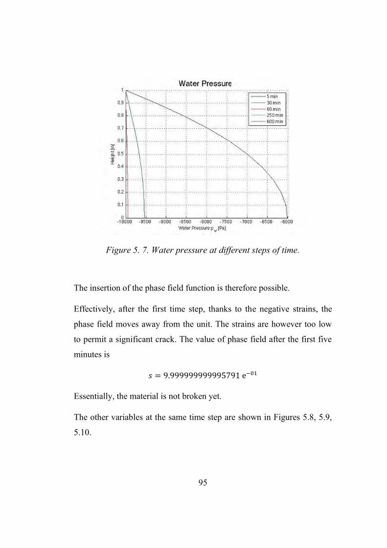
95
Figure 5. 7. Water pressure at different steps of time.
The insertion of the phase field function is therefore possible.
Effectively, after the first time step, thanks to the negative strains, the
phase field moves away from the unit. The strains are however too low
to permit a significant crack. The value of phase field after the first five
minutes is
𝑠 = 9.999999999995791 e−01
Essentially, the material is not broken yet.
The other variables at the same time step are shown in Figures 5.8, 5.9,
5.10.
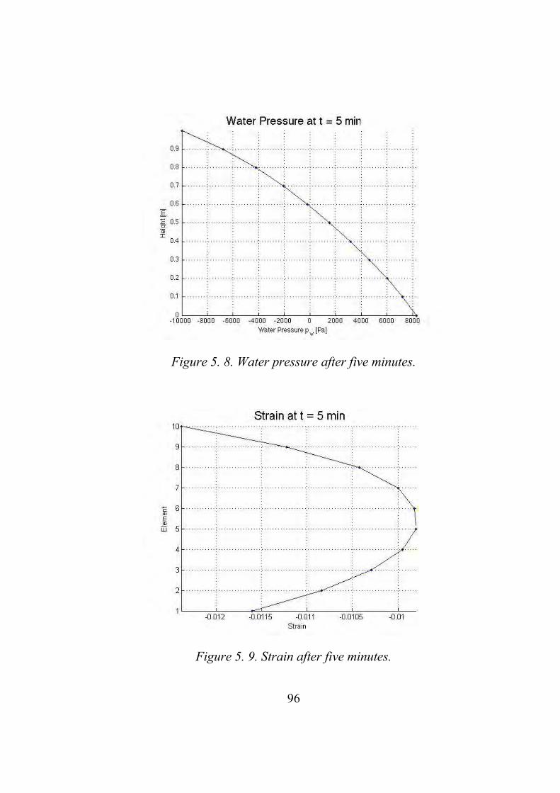
96
Figure 5. 8. Water pressure after five minutes.
Figure 5. 9. Strain after five minutes.

97
Figure 5. 10. Displacements after five minutes.
Going on with the time steps, displacements and strains lightly increase,
but the order of magnitude remains about the same. The phase field
variable remains for this reason unchanged during the evolution in time.
In the next graphs the trend of water pressures, strains and displacements
at different time steps are plotted.
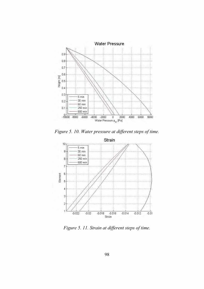
98
Figure 5. 10. Water pressure at different steps of time.
Figure 5. 11. Strain at different steps of time.

99
Figure 5. 12. Displacements at different steps of time.
Clearly, with the value of phase field constant and so closed to zero, the
outputs with insertion of phase field calculation is essentially the same
(or anyway not so different) of those calculated using the porous media
model alone. This is clear in the next Figures 5.13, 5.14, with a
comparison between the two at time 𝑡=5 𝑚𝑖𝑛𝑢𝑡𝑒𝑠.

100
Figure 5. 13. Comparison of pressures with and without phase field.
Figure 5. 14. Comparison of displacements with and without phase field.

101
It is not possible to increase the water pressure imposed on the top
because of the limitation of the Liakopoulous laws for 𝑆𝑤, and
consequently for pressure.
Liakopoulus test, because of its experimental nature, is valid in fact for
saturation degrees not higher than 0,91. This corresponds to a value of
water pressure, that cannot pass an intensity of about 9200 Pa. This
example already lightly overpass the limit. It is not therefore possible to
increase the capillary pressure on the top of the column.
5.2.2. Traction on the top. Ten elements-column.
The second example of union between phase field and the porous media
is the following.
The geometry is the Liakopoulus’ column with the same material
parameters and the same constitutive relations.
On the top a displacement is imposed with an intensity 0,001m every
time step. Water pressures on the bottom of the column are fixed at 9806
Pa. The starting point is the final results or the process of consolidation
(for pressures and displacements).
Because of the same reasons explained in Section 5.2.1., the minimum
water pressure that can be reached using the same constitutive relations
of Liakopoulus test is -9200Pa.
After ten minutes, this limit is already overpassed.

102
In order to show the evolution of the variables (and in particular the
decreasing of the phase field value) over these 10 minutes, the results are
taken for a longer time. Reached the 40 minutes the values of the
variables are clearly distorted.
In the following pages, the results in term of displacements, water
pressure, saturation degree and phase field value, are described with
graphs.
A comparison between the implementation with and without considering
the phase field variable is made.
Displacements
The evolution of displacements during the time taking into account the
phase field (Figure 5.15a) and without considering it (Figure 5.16b) are
shown.
a) b)
Figure 5. 15. Displacements at different steps of time, with (a) and without (b) considering the phase field.

103
The comparison between final displacements considering or not
considering the phase field at some different time steps (5,10,15 minutes)
are now reported.
Figure 5. 16. Displacements after 5 minutes with and without considering the phase field.
Figure 5. 17. Displacements after 10 minutes with and without considering the phase field.

104
Figure 5. 18. Displacements after 15 minutes with and without considering the phase field.
As regards the displacements, the difference between those ones
calculated without taking into account the phase field variable are not so
different (but a little bit inferior) than the ones obtained from the
complete model.
Water pressure
Similarly to what was made for the displacements, also for water
pressures the evolution in time is shown, both in the case complete with
phase field and both in the case with the porous media alone.
The limit imposed for Liakopoulus constitutive laws is highlighted with
a vertical red line (overpassed by the complete model after ten minutes).

105
a) b)
Figure 5. 19. Water pressures at different steps of time, with (a) and without (b) considering the phase field.
The comparison between final displacements considering or not
considering the phase field at some different time steps (5,10,15 minutes)
are now reported.
Figure 5. 20. Water pressures after 5 minutes with and without considering the phase field.

106
Figure 5. 21. Water pressures after 10 minutes with and without considering the phase field.
Figure 5. 22. Water pressures after 15 minutes with and without considering the phase field.

107
Observing the graphs above, the obvious conclusion that can be made is
that water pressures in the complete model with phase field is lower in
modulus. In fact the limit value (when every physical meaning of
constitutive laws is lost) is reached before in the model without the phase
field implementation (40 minutes).
In the complete model this limit is reached after 54 minutes, as shown in
Figure 5.23.
Figure 5. 23. Water pressures after 54 minutes in the complete model.

108
Saturation degree
The evolution in time of Saturation degree is shown in Figure 5.24. In
this case, the red vertical line indicates the limit for 𝑆𝑤, fixed at 0.91.
Figure 5. 24. Saturation degree at different steps of time.
Following, the results at some different time steps (5,10,15 minutes)
Figure 5. 25. Saturation degree after 5 minutes.

109
Figure 5. 26. Saturation degree after 10 minutes.
Figure 5. 27. Saturation degree after 15 minutes.
After 10 minutes, the Saturation degree at the top of the column begin to
overpass the limit. In the case without the phase field implementation
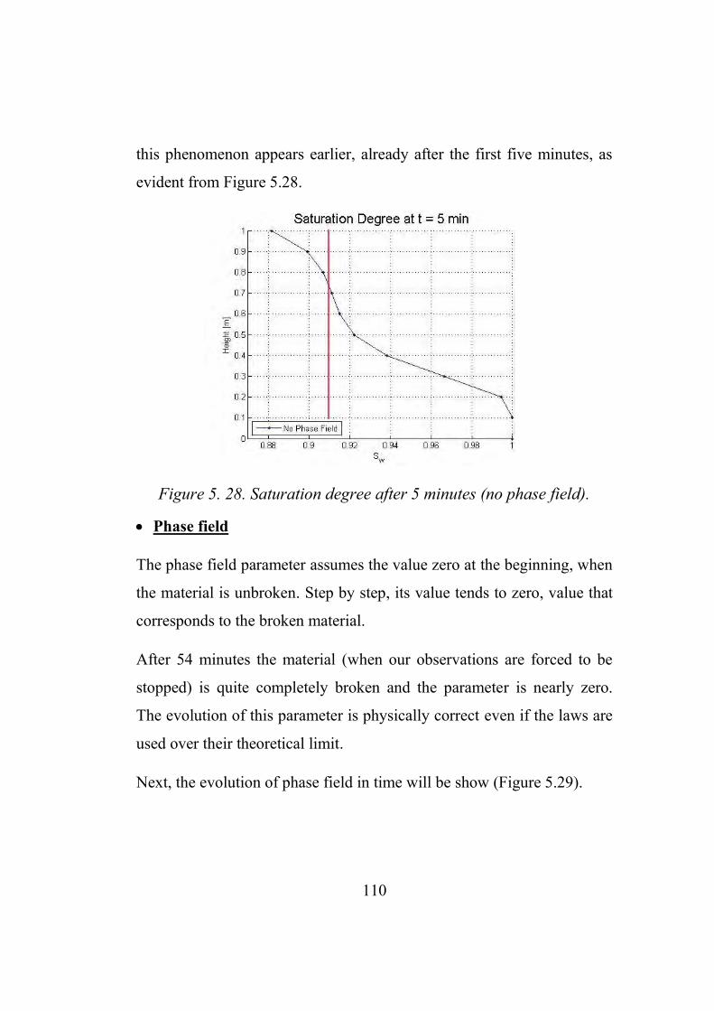
110
this phenomenon appears earlier, already after the first five minutes, as
evident from Figure 5.28.
Figure 5. 28. Saturation degree after 5 minutes (no phase field).
Phase field
The phase field parameter assumes the value zero at the beginning, when
the material is unbroken. Step by step, its value tends to zero, value that
corresponds to the broken material.
After 54 minutes the material (when our observations are forced to be
stopped) is quite completely broken and the parameter is nearly zero.
The evolution of this parameter is physically correct even if the laws are
used over their theoretical limit.
Next, the evolution of phase field in time will be show (Figure 5.29).
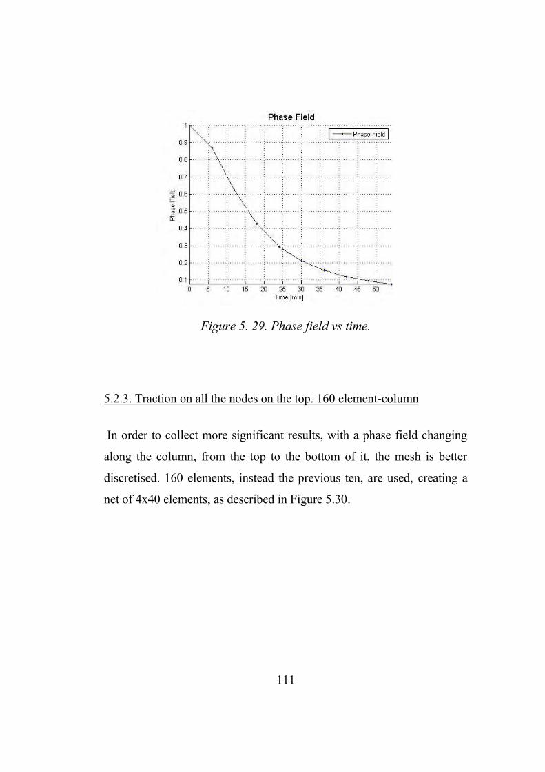
111
Figure 5. 29. Phase field vs time.
5.2.3. Traction on all the nodes on the top. 160 element-column
In order to collect more significant results, with a phase field changing
along the column, from the top to the bottom of it, the mesh is better
discretised. 160 elements, instead the previous ten, are used, creating a
net of 4x40 elements, as described in Figure 5.30.

112
Figure 5. 30. Mesh with 160 elements.
The column is therefore loaded with incremental displacements (0.001 m
each time step) applied on the five superior nodes.
Even in this case the limit pressure for the application of Liakopolus
constitutive relations are overpassed, in order to catch the evolution of all
the variables in time, even after reaching the limit point for pressures.
The inevitable stop is after 35 minutes: after them the Liakopolus laws
lose every physical meaning.
The results at each time step are shown below.

113
t = 5 minutes
Figure 5.31.Results after 5 minutes.
t = 10 minutes

114
Figure 5. 32. Results after 10 minutes.
t = 15 minutes
Figure 5. 33.Results after 15 minutes.

115
t = 20 minutes
Figure 5. 34. Results after 20 minutes.
t = 25 minutes

116
Figure 5. 35. Results after 25 minutes.
t = 30 minutes
Figure 5. 36. Results after 30 minutes.

117
t = 35 minutes
Figure 5. 37. Results after 35 minutes.
Final considerations
Values of phase field change from the top to the bottom of the column.
Obviously the column breaks before in correspondence of the application
of the load.
After the 35 minutes, the deformation of the column is the following:

118
Figure 5. 38. Column configuration after 35 minutes.
The column is stretched, becoming 1.2 meters high: 0.2 meters more
than in the initial conditions. Observing carefully the Figure 5.38, a
different deformation of the elements can be noticed. In particular the
element below are less stretched than the elements above.
An important observation is that after ten minutes water pressure values
have already overpassed the limit pressure of Liakopoulus test.
At the last possible measure (35 minutes) the phase field value has
however reached the value of 0,1632: the material can be considered
almost totally broken.

119
The evolution of the phase field (calculated in one of the nodes of the
top) in time is plotted in the next graph (Figure 5.39).
Figure 5. 39.Phase Field vs Time.
5.2.4. Traction on two the nodes on the top. 160 element-column
This example is a variation of the previous one. The mesh used is the
same with 160 elements. The only difference is the point where the
incremental displacements are applied. Instead of applying it to all the
nodes on the top of the column, it is applied only to the two external
nodes on the top. The aim is to notice a differentiation of strains and
phase field variable even along the horizontal direction.
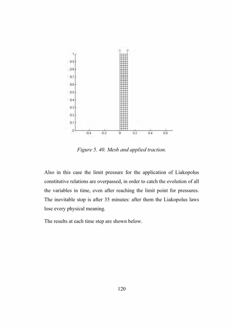
120
Figure 5. 40. Mesh and applied traction.
Also in this case the limit pressure for the application of Liakopolus
constitutive relations are overpassed, in order to catch the evolution of all
the variables in time, even after reaching the limit point for pressures.
The inevitable stop is after 35 minutes: after them the Liakopolus laws
lose every physical meaning.
The results at each time step are shown below.

121
t = 5 minutes
Figure 5. 41. Results after 15 minutes.
t = 10 minutes

122
Figure 5. 42. Results after 10 minutes.
t = 15 minutes
Figure 5. 43. Results after 15 minutes.
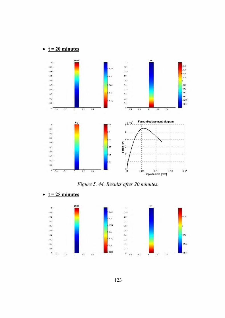
123
t = 20 minutes
Figure 5. 44. Results after 20 minutes.
t = 25 minutes

124
Figure 5. 45. Results after 25 minutes.
t = 30 minutes
Figure 5. 46. Results after 30 minutes.
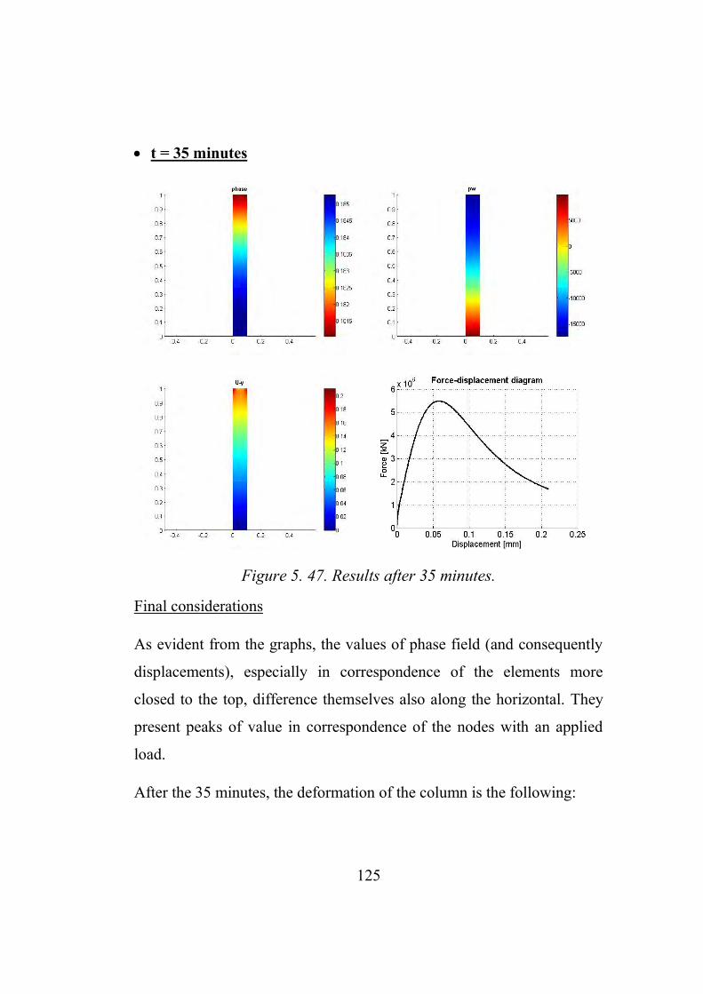
125
t = 35 minutes
Figure 5. 47. Results after 35 minutes.
Final considerations
As evident from the graphs, the values of phase field (and consequently
displacements), especially in correspondence of the elements more
closed to the top, difference themselves also along the horizontal. They
present peaks of value in correspondence of the nodes with an applied
load.
After the 35 minutes, the deformation of the column is the following:

126
Figure 5. 48. Column configuration after 35 minutes.
At the last possible measure (35 minutes) the phase field value has
however reached the value of 0,1815: the material can be considered
almost totally broken.
The evolution of the phase field in time is plotted in the next graph
(Figure 5.49).

127
Figure 5. 49. Phase field vs Time.
It could be now interesting to compare the different evolution of phase
field in the two last cases (traction applied on 5 nodes, or only on two
nodes). This comparison is made in Figure 5.50.
Figure 5. 50. Phase field vs Time – Comparison.

128
The phase field values in both cases are plotted in correspondence of one
of the stretched nodes. The conclusion is that if less nodes are involved
in the traction, they are consequently characterized by a highest value of
phase field. They will arrive earlier to a fracture: this is comprehensible
also from a physical point of view.

129
Chapter 6 – Conclusions
This work began with a carefully itinerary through the complex world of
the phase field. The first weeks in Braunschweig have been devoted to
the analysis of the phase field theory, as well as to the comprehension of
its implementation in the Matlab code, kindly provided by the foreign
Institute.
After that the attention was moved to the discovery of the porous media:
their equations, their features and their laws. This was the indispensable
step to implement a code able to perfectly describe the phenomena just
studied.
Finally, the last stage: to find the right way to fit the two models
together, not only from the point of view of a correct theoretical
approach, but also from a numerical point of view.
The set goal for this master thesis was showing a proof that an union of
the two big fields of research is possible and open the way for future
investigations.
In fact, no studies have still leaded in this direction till now, and the way
is still opened.
After this work, the result in this sense can be considered satisfactory.
With the last examples of Chapter 5 is clear that the two models can
combine in the right way and the number of tests and situation that can
be simulated to examine in depth the subject is really ample.

130
In this work, some limits due to the applicability of the constitutive laws
had to be taken into account. The first step for future analysis will be
therefore the use of different laws which can better and more extensively
describe the phenomena.
The way is opened, hopefully the future and the future studies will
produce other proofs and deeper examples that this bond “porous
media/phase field” is really possible.
131
Bibliography
Borden M.J. et al.; “A phase field description of dynamic brittle
fracture”, Computer Methods Applied Mechanics and Engineering 217-
220 (2012) 77-95
Durner W.;Flühler H.; “Soil Hydraulic Properties”, Encyclopedia of
Hydrological Sciences. Edited by M G Anderson. 2005 John Wiley &
Sons, Ltg.
Kuhn C.; “Investigation of a Phase Field Model for Fracture”,2013
Lewis R.W.; Schrefler B.A.; “The Finite Element Method in the Static
and Dynamic Deformation and Consolidation of Porous Media”, 1998
John Wiley & Sons, Ltg.
Lu N.; Likos W.J.; “Unsaturated Soli Mechanics”, 1960 John Wiley &
Sons, Ltg.
Miehe C. et al.; “A phase field model for rate-independent crack
propagation: Robust algorithmic implementation based on operator
splits”, Computer Methods Applied Mechanics and Engineering 199
(2010) 2765-2778
Xie
Zienkiewicz O.C.; Chan A.H.C.; Pastor M.; Schrefler B.A.; Shiomi T.;
“Computational Geomechanics, with special Reference to Earthquake
Engineering; John Wiley & Sons, Ltg.


![[Vicino Oriente XIX (2015), pp. 85-96]...Keywords: Fayyūm; Bakchias; Early Christianity; church architecture; monasticism 1. EARLY CHRISTIANITY IN THE FAYYŪM: LITERARY SOURCES AND](https://static.fdocuments.us/doc/165x107/60651ae67e5bc723d85b3114/vicino-oriente-xix-2015-pp-85-96-keywords-fayym-bakchias-early-christianity.jpg)