A numerical and experimental study on turbulent

natural convection in a differentially heated cavity

Driek RouwenhorstEngineering Fluid Dynamics

University of TwenteThe Netherlands

d.rouwenhorst@student.utwente.nl

Florianopolis, Brazil, 03/2011 - 07/2011

Supervisor POLO: Prof. Cesar J. Deschamps

Supervisor UT: Prof. dr. ir. H.W.M. Hoeijmakers

Report of internship activities at POLO, Research Laboratories forEmerging Technologies in Cooling and Thermophysics.

Abstract

The three-dimensional flow field and temperature distribution in adifferentially heated vertical cavity is identified by means of different nu-merical models and experimental measurement techniques. Numerically,the performance of different turbulence models are validated with DNSdata available in literature. The main results will be published in theXXXII Iberian Latin-American Congress on Computational Methods inEngineering (CILAMCE). A model with sufficient performance will beused to simulate the flow in the experimental setup to give an accuratedescription of the phenomenon. Along specific contours the velocity fieldis measured experimentally in two dimensions applying Laser Doppler Ve-locimetry (LDP). For a more global overview of the flow behavior ParticleImage Velocimetry (PIV) is used in some cross-sectional planes. In addi-tion, the temperature distribution in the flow is visualized exploiting theLiquid Crystal Thermography (LCT) measurement technique. Finally,the heat flux distribution from the heated walls to the fluid is obtainedby the positioning of an array of flux sensors. The classifying Rayleighnumber is defined by the height of the cavity, which is related to its squarebase by an aspect ratio of four. Numerically RaH = 6, 4 · 108 and 1010

are considered with air as working fluid (Pr = 0.71), making it possibleto compare the results with available DNS data. In the experiments wa-ter is used (Pr = 7.0) and is exposed to a temperature difference suchthat RaH = 1 · 1010 is achieved, where the flow is measured with thenon-intrusive techniques. The experimental results will complement ex-isting data at lower Rayleigh numbers available in literature. The mainobject is to extend the availability of accurate experimental data on natu-ral convection in differentialy heated cavities. This data can be exploitedto validate different numerical methods, trying to capture the behavior ofturbulent natural convection in the most efficient way. The work under-lined above is the graduation project of Andre Popinhak, in which I wasassigned to assist. The activities had already begun before the internshipstarted and was not finished before the end of this period, therefore thesubjects descibed are representative for the learned theory and performedtasks of the internee rather then a complete description of the researchcarried out.

Keywords: Natural convection; Turbulence; Cavity; LDV; LCT

1

Contents

1 Introduction 4

2 Theory 52.1 Governing equations . . . . . . . . . . . . . . . . . . . . . . . . . 52.2 Turbulence modeling . . . . . . . . . . . . . . . . . . . . . . . . . 6

2.2.1 Time averaging . . . . . . . . . . . . . . . . . . . . . . . . 62.2.2 Closure problem . . . . . . . . . . . . . . . . . . . . . . . 72.2.3 Mixing length . . . . . . . . . . . . . . . . . . . . . . . . . 72.2.4 k − ε model . . . . . . . . . . . . . . . . . . . . . . . . . . 72.2.5 Reynolds stress equation model (RSM) . . . . . . . . . . . 82.2.6 Large eddy simulation (LES) . . . . . . . . . . . . . . . . 82.2.7 Wall treatment . . . . . . . . . . . . . . . . . . . . . . . . 8

3 Numerical simulation 103.1 Solution procedure . . . . . . . . . . . . . . . . . . . . . . . . . . 103.2 SST k − ω model . . . . . . . . . . . . . . . . . . . . . . . . . . 113.3 RSM . . . . . . . . . . . . . . . . . . . . . . . . . . . . . . . . . . 113.4 Conclusions . . . . . . . . . . . . . . . . . . . . . . . . . . . . . . 113.5 Large eddy simulation . . . . . . . . . . . . . . . . . . . . . . . . 14

3.5.1 Mesh design . . . . . . . . . . . . . . . . . . . . . . . . . . 143.5.2 Journal file . . . . . . . . . . . . . . . . . . . . . . . . . . 153.5.3 Solution procedure . . . . . . . . . . . . . . . . . . . . . . 15

4 Experimental setup 174.1 Cavity . . . . . . . . . . . . . . . . . . . . . . . . . . . . . . . . . 17

4.1.1 Environment . . . . . . . . . . . . . . . . . . . . . . . . . 174.1.2 Radiation . . . . . . . . . . . . . . . . . . . . . . . . . . . 174.1.3 Thermal boundary conditions . . . . . . . . . . . . . . . . 17

4.2 Measurement instrumentation . . . . . . . . . . . . . . . . . . . . 184.2.1 Positioning system . . . . . . . . . . . . . . . . . . . . . . 184.2.2 LDV . . . . . . . . . . . . . . . . . . . . . . . . . . . . . . 184.2.3 PIV . . . . . . . . . . . . . . . . . . . . . . . . . . . . . . 184.2.4 LCT . . . . . . . . . . . . . . . . . . . . . . . . . . . . . . 184.2.5 Wall heat flux measurement . . . . . . . . . . . . . . . . . 19

5 Laser Doppler Velocimetry 205.1 The optic system . . . . . . . . . . . . . . . . . . . . . . . . . . . 205.2 Test measurements . . . . . . . . . . . . . . . . . . . . . . . . . . 21

5.2.1 half-height, low turbulence . . . . . . . . . . . . . . . . . 225.2.2 80 percent height, high turbulence . . . . . . . . . . . . . 24

6 Particle Imaging Velocimetry 27

2

7 Liquid Crystal Thermography 287.1 Camera procurement . . . . . . . . . . . . . . . . . . . . . . . . . 287.2 Image filtering . . . . . . . . . . . . . . . . . . . . . . . . . . . . 287.3 Conversion to temperature . . . . . . . . . . . . . . . . . . . . . . 30

7.3.1 One-parameter correlation . . . . . . . . . . . . . . . . . . 307.3.2 Neural networks . . . . . . . . . . . . . . . . . . . . . . . 31

7.4 Calibration . . . . . . . . . . . . . . . . . . . . . . . . . . . . . . 31

8 Heat Flux 33

9 Conclusions 349.1 Postscript . . . . . . . . . . . . . . . . . . . . . . . . . . . . . . . 34

10 Appendix A 35

3

1 Introduction

Natural convection is a phenomenon occurring in every environment containinga fluid with temperature gradients, provided that the density is a function ofthe temperature. In many engineering applications the contribution of naturalconvection can be disregarded because often the contribution to the flow behav-ior is negligible when compared to forced convection. Yet there is still a varietyof engineering problems concerned with natural convection, such as convectionin a double glazed window, which increases heat transfer.

For convenience, research on natural convection is often carried out on rect-angular enclosures, as it is a simple geometry for both the experimental andnumerical approach. Several results are available for laminar natural convec-tion in cubical enclosures with heated sides, bottom or positioned under an anglewith respect to the direction of gravity. The case considered in the present re-search deals with heated side walls, referred to as differentially heated walls. Inearlier investigations it has been found that current numerical methods usuallydo not predict the temperature stratification in the core region of the cavitycorrectly [1]. In order to increase the realizability of the boundary conditions inexperiments with air filled cavities, a linear temperature distribution is usuallyproposed instead of the adiabatic assumption [2]. Other experimental investi-gations provide benchmark data for the validation of numerical codes [3],[4].

The range of experimental data is mainly restricted to the laminar and lowturbulent flow regimes. As in the majority of engineering flow problems tur-bulence is involved, it would be desirable to extend experimental data to caseswith higher turbulence intensity. Because the solving of the Navier-Stokes equa-tions with turbulent effects requires a very fine grid and small time steps, directnumerical simulations (DNS) are computationally too costly for engineeringpurposes. Instead, time averaging of the equations is usually employed, elimi-nating the need to solve the time dependency caused by turbulence. However,this approach yields additional unknowns that have to be estimated through aconveniently chosen turbulence model. The method to choose strongly dependson the problem at hand and new methods for broader application and betterperformance are continuously sought. Therefore there is a need for experimentaldata on turbulent flows for validation purposes, which are too scarce at the mo-ment. Despite the geometric simplicity, differentially heated cavities provideschallenging features for numerical modeling, because of the presence of turbu-lence and steep gradients near the walls and a nearly stagnant core region.

Accurate DNS calculations also prove to be good validation material andwere performed on a cavity with aspect ratio four [5], similar to the geometryconsidered in this work. Different levels of turbulence are considered, using theparameter Pr = 0.71 to resemble the flow of air. In the present experimentalresearch a matching degree of turbulence is aimed for using water, thereforecomplementing the data with results for Pr = 7.0.

4

2 Theory

Obviously the velocity and temperature distributions in a differential heatedenclosure can not be solved analytically. In such cases the analysis can becarried out by using either experiments or applying an appropriate numericalmethod. Several variables are involved and it is a common practice to reducethem to a few dimensionless numbers. With the use of the Buckingham Πtheorem, the number of variables governing a specific problem can be narroweddown to just a few dimensionless numbers. In the case of natural convectionthe most important number is the Rayleigh number, describing the qualitativeratio between buoyancy forces and viscous forces:

RaH =gβ∆TH3

να(2.1)

with α being the thermal diffusivity and β the thermal expansion coefficient ofthe fluid. In the case of the cavity considered herein, the temperature differencebetween the heated walls is used and the height H is recognized as the relevantlength scale. The driving forces of the natural convection appear in the numer-ator of the Rayleigh number, so the higher the Rayleigh number, the strongerthe natural convection. Geometrically similar problems will show transitionfrom laminar to turbulent natural convection at the same Rayleigh number in-dependent of the fluid used. The transition in a differentially heated cavityoccurs around Ra = 2 · 108, somewhat depending on the surface roughness.Furthermore the solution depends on the Prandtl number:

Pr =µcpk

(2.2)

The Prandtl number describes the ratio between the momentum diffusivity tothe thermal diffusivity. As heat is the driving force for the momentum boundarylayer, the Prandtl number has an important influence on natural convection,affecting the thickness of the momentum and thermal boundary layers. Mostfound Prandtl numbers in literature are those of water and air at atmosphericcondition, being close to 7 and 0.7, respectively.

2.1 Governing equations

As the expected velocities in the solution are expected to be very low comparedto the speed of sound in the fluid and the temperature difference between thevertical walls is small, a good starting point would be the incompressible Navier-Stokes equations. The PDE conservation forms of such governing equations are:

∂~u

∂t+ ~u · ∇~u = −1

ρ∇p+ ν∇2~u+ ~g (2.3)

Provided that the gravitation vector is the only source of body forces. Incom-pressibility reduces the continuity equation to the following expression:

∇ · ~u = 0 (2.4)

5

Because the flow is driven by temperature differences, the energy equation needsto be considered too:

ρ∂E

∂t+ ρ∇ · (~uH) = ρ~u · ~f +∇ · (¯τ~u) +∇ · (k∇T ) + Q (2.5)

Note that despite incompressibility is assumed, the buoyancy forces are takeninto account through a thermal expansion coefficient that gives rise to the bodyforce ~f . These five equations can be rewritten into a general form with the con-served variable φ that can be solved with commercial software, such as Fluent,applying the finite volume method [6].

∂φ

∂t+∇ · (φ~u) =

1

ρ∇ · (Γ∇φ) +

1

ρSφ (2.6)

The left side of equation 2.6 represents the local increase of the variable in timeand the convective outflow of the fluid element. This is forced to be equal tothe increase of the variable by the diffusion and the volumetric source term onthe right side.

2.2 Turbulence modeling

The governing equations could be solved directly without applying a model forturbulence. However, in order to capture the physics, an unsteady simulationwith small time steps should be applied on a very fine grid, taking months ona simple problem in order to have enough data to perform statistics on theturbulence.

2.2.1 Time averaging

Usually one is not interested in the behavior of individual eddies in a turbulentflow, but rather wants to know the mean behavior and the occurring deviationsbecause of these eddies. For this purpose the variables are decomposed into atime averaged part and the fluctuating part caused by the turbulence, beforesubstitution in the governing equations. Lets consider the decomposed velocityvector ~u = ~U + u′ and the decomposed pressure p = P + p′, substituted theminto the momentum equations 2.3 and see what happens when the terms areaveraged in time:

∂(~U + ~u′)

∂t+ (~U + ~u′) · ∇(~U + ~u′) = −1

ρ∇(P + p′) + ν∇2(~U + ~u′) + ~g (2.7)

By definition the averages of the fluctuating parts are zero when appearing inlinear forms, simplifying the above expression to:

∂~U

∂t+ ~U · ∇~U + ~u′ · ∇~u′ = −1

ρ∇P + ν∇2~U + ~g (2.8)

Bringing us back to the same momentum equations 2.3 but for the six introducednon-linear terms of the perturbations in the velocity field ~u′ · ∇~u′, referred to

6

as the Reynolds stresses. Applying the same strategy to the energy equation2.5 yields three similar terms representing correlations between temperature andvelocity perturbations. Note that the continuity equation 2.4 does not change inthis evaluation, the velocity components are just replaced by the time averagedvelocities.

2.2.2 Closure problem

The new set of equations are called the Reynolds Averaged Navier-Stokes equa-tions (RANS). The new terms, consisting of the fluctuations in the velocitycomponents and temperature are unknown and pose the closure problem of theRANS equations.

Observations of turbulent flows showed that the largest values of the fluc-tuations in the velocity field are found in the regions where the mean velocitygradient is largest. This has led to the Boussinesq approximation, relating theReynolds stresses to mean flow velocity gradients with a viscosity-like constantµt called the turbulent viscosity.

τij = −ρu′iu′j = µt

(∂Ui∂xj

+∂Uj∂xi

)(2.9)

The analogous turbulent transport of the thermal energy takes the form

−ρu′iT ′ = kt∂T

∂xi(2.10)

Usually the assumption is made that the turbulent temperature diffusivity isequal to a fraction of the turbulent viscosity σtkt = µt, defined by the turbulentPrandtl number σt. The only thing left now is to find a proper expression forthe turbulent viscosity and the closure problem is solved.

2.2.3 Mixing length

The first attempt to find an expression for the kinematic turbulent viscosity νtwas by means of dimensional analysis. The dimensions [m2/s] were sought bythe multiplication of physically relevant length and velocity scales, yielding

µt = ρνt = ρl2m

∣∣∣∣∂U∂y∣∣∣∣ (2.11)

which proved pretty accurate for simple two-dimensional flows. The length scaleis a combination of the physical relevant length and an experimentally obtainedconstant belonging to a certain problem. This method is called Prandtl’s mixinglength model.

2.2.4 k − ε model

In an attempt to develop a model that is more generally applicable, the k − ε-model was developed. The model computes the turbulent viscosity from two

7

more variables that are solved in the domain. One equation for the turbulentkinetic energy k = 1

2 |~u′|2 and another for the viscous turbulence dissipation are

assembled to the best knowledge of the physical behavior. In these equationsfour adjustable constants are present that are set to a value such that a widerange of turbulent flows is solved accurately. A fifth constant is found in theequation of the turbulent viscosity from k and ε: µt = ρCµk

2/ε. This is thesimplest general model to close the RANS equations, supplying reasonable re-sults for some engineering applications. The main drawback for this methodand variations on it like the k − ω method, lies in the fact that it assumes theturbulent viscosity to be an isotropic scalar, which is not accurate for flows withfor example complex strain fields or significant body forces.

2.2.5 Reynolds stress equation model (RSM)

The more complex turbulence model RSM solves transport equations for all sixindependent Reynolds stresses instead of just the kinetic energy. The turbu-lent dissipation ε needs to be resolved, yielding seven equations for the modelrequired to solve the turbulent flow. This method is the most general of theclassical turbulence models, but computational costs are considerably highercompared to k − ε. The major uncertainty comes from the modeling of theturbulent dissipation [6].

2.2.6 Large eddy simulation (LES)

LES can be considered as an efficient midway between the computational costlyDNS and turbulence models based on the RANS approach. The large eddies,containing most of the turbulence kinetic energy, are resolved directly, whilethe more isotropic behaving, low-energy containing small eddies are modeledapplying the Boussinesq approximation. The mesh resolution generally acts asthe filter to separate these two scales and therefore determines the smallest eddythat will be resolved. On one hand computational cost is much higher than evenRSM, but on the other hand it is way lower than for a full DNS simulation.

2.2.7 Wall treatment

When a turbulent flow is bounded by a wall, this will affect the turbulent quan-tities. The no-slip and impermeability conditions not only apply to the mainflow, but also to the fluctuations. On the other hand the velocity gradient nearthe wall will act like a source of turbulence. Good near-wall modeling is there-fore in general very important, while most turbulence models are developed topredict free-stream turbulent behavior [7].

A turbulent boundary layer can be subdivided into a viscous sublayer verynear the wall where molecular diffusion plays a dominant role, fully-turbulentregion further away from the wall, and a transition region between them. Thesolution can be solved up to the wall, but this requires a very fine mesh for thehigh gradients in the mean and turbulent quantities. At least some volumes

8

must lie within the viscous sublayer for accurate results. Another approach isto apply wall functions, semi-empirical functions describing the behavior of theturbulent quantities near the wall. This approach obviates the need of a veryfine mesh to solve the boundary layer, which might drastically reduce compu-tational time. However, special care has to be given to the validity of the wallfunctions for the type of flow being considered, which can include effects asstrong adverse pressure gradients.

9

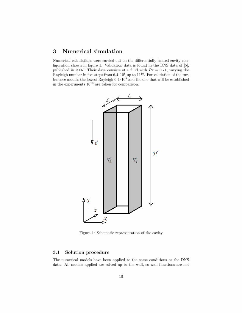
3 Numerical simulation

Numerical calculations were carried out on the differentially heated cavity con-figuration shown in figure 1. Validation data is found in the DNS data of [5],published in 2007. Their data consists of a fluid with Pr = 0.71, varying theRayleigh number in five steps from 6.4 ·108 up to 1110. For validation of the tur-bulence models the lowest Rayleigh 6.4 ·108 and the one that will be establishedin the experiments 1010 are taken for comparison.

Figure 1: Schematic representation of the cavity

3.1 Solution procedure

The numerical models have been applied to the same conditions as the DNSdata. All models applied are solved up to the wall, so wall functions are not

10

applied. First laminar calculations are performed by setting the gravitationalconstant a factor 100 lower. This solution is used as initial guess for the turbu-lence models. After convergence is reached, velocity, temperature and turbulentintensity values are read and compared along certain lines in the domain. Thesolutions have been verified for truncation error, by means of mesh-refinementtests. A grid size of 100x250x50 (x,y,z) proved to be sufficient. The calculationsare all conducted by the commercial code Ansys Fluent 12.0.

3.2 SST k − ω model

The first and simplest model considered is the Shear-Stress Transport (SST)k − ω model. The model k − ω differs from the briefly described k − ε modelin that it resolves for the specific dissipation rate ω, rather then the turbulencedissipation rate ε which has proven to be more accurate for wall-bounded flows.The SST adopts the k − ω model near the wall and the k − ε model furtheraway from the walls, making the model more generally applicable compared tothe standard k − ω. The result of velocity and temperature profiles at 20, 50and 80 percent of the height of the cavity is shown in figure 2 and 3.

3.3 RSM

The second model applied is the RSM model. The converged solution of thek−ω model served as the initial guess for this more advanced model. This modelshould be able to produce better results near the wall and in the corners wherethe streamline curvature is relatively high. These results are also included infigure 2 and 3.

3.4 Conclusions

At the lower turbulence intensity both models show pretty good agreementwith the DNS data, the k − ω model seems to overestimate the momentumdiffusion and RSM overestimates the maximum velocity. Both models slightlyunderestimate the temperature stratification over the cavity hight. Also theresults for the local Nusselt number along the heated walls are accurate forthe lower Rayleigh number, see figure 4. At the higher Rayleigh number thedeviations in the velocity between the models and the DNS are unacceptablyhigh.

Of course the best variables for the validation of turbulence modeling arethe turbulence quantities, like the turbulence intensity It = k

1/2|~U |2. For the

k − ω model the magnitude of the turbulence intensity is accurate, but thedistribution is not, probably because the turbulence is modeled by two equationsonly. Although the solution of the RSM appears to be more accurate, strangelythe turbulence intensity is found to be virtually zero in the hole domain. In fact,for an unknown reason, the model finds a laminar solution for the problem,explaining the over-prediction of the velocity because there is no additionalviscous dissipation as a result of the turbulence.

11

Figure 2: Comparison of velocity and temperature profile at RaH = 6.4 · 108

12

Figure 3: Comparison of velocity and temperature profile at RaH = 1010

13

Figure 4: Local Nusselt number along the heated wall, RaH = 6.4 · 108

3.5 Large eddy simulation

Since the RSM was found unable to capture the turbulence quantities in thesolution, LES was also carried out in the present study. As the computationalefforts are some magnitudes of order higher than the previous models that soughta steady state solution, the computational power of a cluster is exploited.

3.5.1 Mesh design

The mesh used for the LES model is developed with the use of the validationdata. As the mesh size determines the size of the resolved eddies, it is importantto use a fine and consistent grid in the region with high turbulence intensity. Amesh density function is chosen based on the turbulence kinetic energy. Figure5 shows the turbulence kinetic energy at the lower Rayleigh number with thedensity function scaled to the same order of magnitude.

Near the wall a constant distribution is used and in the middle of the cavitythe density is 20 times lower. A smooth transition is applied between thoseregions. The turbulent kinetic energy for the high Rayleigh number has similarmagnitude, but is located closer to the wall. With this density function 150points are distributed in the x-direction between the heated walls. In the otherdirections bi-exponential density functions are applied, yielding close to cubicvolumes in the cavity core and a fine distribution near the walls, placing thefirst volume well within the viscous sublayer.

14

Figure 5: Turbulence kinetic energy and the density function for the LES-mesh

3.5.2 Journal file

The Fluent application running on the cluster is controlled by a sequence ofcommands listed in a so-called journal file. In order to export variable datafor every time step and apply autosave, loops had to be written in Schemeprogramming language which is supported by Fluent. With the help of [8] ajournal file could be written to retrieve the required data automatically.

Moreover Matlab codes were written to read the data for the calculationof the statistical variables and visualize physically relevant variables such asisocontours of temperature and Reynolds stresses. A screen-shot of a resultingmovie of temperature profiles in the top quarter of the cavity is shown in figure6.

3.5.3 Solution procedure

An attempt was made to solve the problem explicitly, being computationallycheap for solving with small time steps. Unfortunately the solution did notconverge, even for very low Courant numbers. Instead the implicit scheme isused, roughly requiring a week to gather enough data for statistically stablesolution on a cluster node with eight processors. Due to some problems withthe cluster there are no statistically stable results yet to show.

15

Figure 6: Temperature isocontours in the top of the cavity, LES RaH = 6.4 ·108

16

4 Experimental setup

The cavity, shown in figure 1, has a square base and an aspect ratio of 4, givingit the dimensions 100x400x100 mm. The cavity is positioned vertically, aligningthe longest side with the y-axis. As the gravitational force acts along the y-axis, the Rayleigh number is based on the height H. The temperature of thealuminum walls perpendicular to the x-axis can be controlled in order to applythe differential heating to the cavity. The front, back, top and bottom of thecavity are constructed from PMMA, enabling optical measurement techniquesto retrieve data. The fluid to be studied in the cavity is water.

4.1 Cavity

This section describes the positioning of the cavity in the laboratory. Thetemperature management is considered and special attention is given to thethermal boundary conditions defining the problem and creating the possibilityto compare the experimental results to future numerical calculations.

4.1.1 Environment

The ambient temperature inside the laboratory is kept constant at 20◦C bythe air conditioning system, with an accuracy of 1◦C. The cavity is placedon a suspended table, isolated from external vibrations (heavy traffic, work-ing laboratory technicians etc.) by a set of springs. The setup is shielded byblack curtains, primarily for the safety of the laboratory technicians, but it alsoprevents ambient light to influence the measurements.

4.1.2 Radiation

With water as the applied working fluid, the used dimensions guarantee a tem-perature difference of around 10◦C in order to reach the turbulent flow regimeup to the aimed value of RaH = 1010. Combined with the low emissivity of thealuminum heating walls, this assures that radiation will be negligible comparedto the heat flux caused by the natural convection.

4.1.3 Thermal boundary conditions

Heated walls The desired boundary condition of the heated walls is a uni-form temperature. This condition is approached by the high conductivity of thealuminum wall material, kept at temperature by a steady supply of water froma thermostatic bath meandering trough canals embedded in the walls. Measure-ments with thermocouples show a maximum deviation of 0.6◦C from the aimedisothermal temperature.

Remaining walls The non-heated walls are meant to behave adiabatically.The measurement techniques require the walls to be transparent, making goodisolating properties hard to achieve. A high thermal resistance is established

17

by the use of one inch thick PMMA walls instead of the better heat conductingglass alternative. Moreover a low heat flux trough the sidewalls is guaranteedby the small temperature difference of the flow with respect to the controlledambient temperature.

4.2 Measurement instrumentation

For the LDV, PIV and LCT measurements, instrumentation is positioned aroundthe cavity. In order to be able to capture the desired data, the instrumentationthat has to be repositioned is mounted on a positioning table with three remotecontrolled translational degrees of freedom.

4.2.1 Positioning system

The positioning system used is the T3D Standard Traverse System of TSI,specially designed for applications such as LDV and PIV measurements. Thesystem is remote controlled by computer and is integrated with the measurementcontrol of the LDV and PIV systems. The three axis can be positioned over arange of 600mm with an accuracy of 300µm and a repeatability of 10µm. Theprofiles which are part of the table assures flexible use and a rigid fixture of theinstruments.

4.2.2 LDV

The Laser Doppler Velocimetry instrumentation consists of a laser with a mul-ticolor beam separator and a transmitting probe with integrated receiver. Theprobe is connected to the beam separator with a flexible cable and can thereforebe positioned freely by the table to measure the points of interest within the cav-ity. The same probe collects the data by the backscatter of the seeding particlespassing the focal point. Particles reflect the laser light with a certain frequencycaused by crossing a fringe pattern, hence the velocity can be calculated. Thedata is processed by the Photo Detector Module and Signal Processor before itcan be accessed on the computer with FlowSizer software.

4.2.3 PIV

For the Particle Image Velocimetry another laser, emitting a white light, is fixedto the positioning table. The laser illuminates a cross-sectional plane in thecavity from above. A static camera captures the illuminated seeding particles(larger than the particles used for LDV) in a frequency so that the velocity canbe constructed with by correlation between the particles in the images. Thewanted data can be obtained by PowerView software.

4.2.4 LCT

The Liquid Crystal Thermography technique uses encapsulated crystal seedingparticles that change color according to the temperature in a certain range. A

18

sheet of white light from a bright lamp above the cavity defines the plane ofinterest, as in the PIV experiment. A 3CCD camera captures the color field,that - after proper calibration - can be converted numerically to a temperaturefield.

4.2.5 Wall heat flux measurement

For the measurement of the wall heat flux at the heated walls of the cavity,walls with integrated heat flux sensors are installed. These walls are not usedin the other experiments, because the use of these sensors might introduce anadditional error in the uniform temperature of the heated walls that can un-necessarily compromise the accuracy of the other measurement techniques. Awall contains eight sensors distributed over the height, making it possible tocalculate the Nusselt number along the wall.

19

5 Laser Doppler Velocimetry

LDV is the first experiment to be carried out. The setup was used before in thelaboratory and all components were still in place and connected. The settingsthough had to be re-optimized and optical components had to be checked andcleaned. The details of the used instruments for LDV is listed in Appendix A.

5.1 The optic system

The heart of the setup is an argon ion laser, emitting a beam consisting ofspecific wavelengths. Because of the high power requirement of such a laser, itis equipped with water cooling. Approximately ten liters of filtered water perminute is used to remove excess heat. A beam splitter extracts two wavelengthsfrom the laser beam that will be used to measure the two velocity components.A Bragg cell divides these wavelengths in two, with a shift in frequency betweenthe pairs. The two pairs of laser light leaving the beam splitter are led intoindividual optic fibers by couplers. The fibers transport the beams to the probethat is dynamically positioned on the traverse system in front of the cavity.

After the beam splitter was properly aligned with the laser, the couplers hadto be adjusted so the light is focused precisely at the entrance of the fiberglass.Thereto a focusing ring and a course and a fine set of positioning knobs areavailable on the couplers to steer the green (514.5 nm) and blue (488 nm)light that is used. A laser power meter is put in front of the probe allowing tomaximize the efficiency of every coupler. The argon ion laser itself is adjusted tooptimize the combined intensity of the beams. The power of both wavelengthsare found to be of the same order of magnitude.

For proper functioning of the LDV, the pairs of beam paths have to crossexactly at the focal point. Here fringes will develop because of interferencebetween the paired beams. The misalignment of beams in the crossing pointis found to fall within the specifications. The frequency shift induced by theBragg cell in the beam splitter causes the fringes to travel with a constantvelocity within the oval focus point.

Another important feature of the beams is the polarity of the light. In orderto obtain a sharp contrast between the fringes, the polarity of the pairing beamsneed to be similar. The polarization angle of a beam is found with a PolarizationAxis Finder, the angles were assessed to be very accurate. The amount ofpolarization is not very high, but believed to be sufficient, this property isfound by the contrast of the image created with the Polarization Axis Finder.

The fact the measurements are carried out through a window and in anothermedium give extra complications. Refraction and reflection of the laser beamshave to be considered for valid measurement results. Luckily the the solutionsare straightforward in the case the probe is placed perpendicular with respectto a flat window, and also applicable for small offset angles. Reflections fromthe PMMA walls will fall exactly on the same line as from where they weresent. In order to prevent these reflections to influence the measurements fromparticles passing through the focal point, a mask is made that is placed in front

20

of the probe, masking the horizontal and vertical lines between the emittedbeams. The focal point itself is not influenced by the media because of theperpendicularity, only the focal length changes with the distance to the window[9]:

F = FDtanκatanκf

+ t

[1− tanκw

tanκf

]+ d1

[1− tanκa

tanκf

](5.1)

In this expression the new focal length is expressed in the lens’s focal distance,the wall thickness and the probe’s distance to the window. The variable κ is thehalf angle between the beams in the air, window and fluid respectively. We areinterested in the displacement of the focal point with respect to a displacementof the probe. Thereto we differentiate the expression with respect to the distanceto the window: dF

dd1= 1− tanκa

tanκf. The angle of the beams in the fluid is found with

Snell’s law κf = sin−1 (sinκa ·Na/Nf ), as a function of the refractive indexes.Recognizing that the displacement of the focal point is the displacement of theprobe plus the change of focal distance yields:

dxFdxP

=

√(Nf

Na cosκa

)2

− tan2 κa = 1.33 (5.2)

So put in words, the focus point travels one third faster than the probe in thez-direction. This result will be used for positioning the focal point to the desireddepth in the cavity.

5.2 Test measurements

To get acquainted to the measurement technique and find the optimal con-ditions, some test measurements are carried out on a prototype cavity. Thequantity that will be measured is the frequency content of the backscatteredlight. When a particle crosses the focal point of the laser beams this causesan increased intensity. The frequency of the passing of a particle will be upto about the kHz range, depending on its velocity. A higher frequency will besuper-positioned on this signal because of the moving fringes within the focalpoint. This signal will be in the MHz range; the 40 MHz of the shift appliedby the Bragg cell plus the Doppler effect as a result of the particle velocityperpendicular to the fringes. Above this order of magnitude in the frequencythe noise will prevail.

For seeding, polyamide particles are suspended in the flow with an averagediameter of 5µm. The particles have a density very close to the density of wa-ter, making them follow the flow accurately. Because of the low velocities in theexperiment the passing frequency of the particles through the focal point is alsolow. This cannot be overcome by increasing the amount of particles, when toomuch particles are used the water is saturated and the seeding particles settleat the top wall. Also larger particles are available, but they will span severalfringes, reducing the quality of the signal. In order to obtain a higher data rateit is attempted to measure while moving the probe along the line of measure-ments, hoping more particles would cross the focal point. Unfortunately the

21

data rate did not increase while it did bring other complications, therefore thisstrategy was rejected.

The signal processing equipment will first filter out the particle passing fre-quency with a high pass filter of 20 MHz. Subsequently the signal frequencycan be ’downmixed’, the subtraction of a fraction or the entire 40 MHz shift.This allows the Doppler frequencies, containing the velocity information, to fallin a certain Band Pass Filter range. The smaller the range can be chosen, thebetter the resolution of the resolved velocity will be.The maximum velocity tobe expected is about 7 mm/s and the fringe spacing for the used blue light is3.73 µm. The maximum Doppler frequency will therefore be about 2 kHz. Thisassures that the boundary layer at one side of the cavity can be fitted exactlywithin the smallest frequency range available, when leaving a 1 kHz shift withthe downmixing.

The most interesting region of the flow is of course the boundary layer, verynear the wall. The measurement technique though uses an angle for the crossingbeams. So to measure the horizontal velocity up to the wall an angle of at least4 degrees is required, directing the focusing point to the wall. This implies thatthe entire profile, from wall to wall cannot be measured in one run, because theprobe needs to be turned say ten degrees to capture both walls. Therefore itwill be more convenient to measure both sides from the wall to the middle andconnect both profiles with post-processing. Because of the angle the measuredvelocity is a combination of the z- and x-direction. As the z-velocities in thecavity are expected to be small compared to the other components and the usedangle will be small, the contribution of the z-component will be neglected. Asmall investigation is carried out for the dependency of the results on the offsetangle about the y-axis. Results of measuring perpendicular and with a 10◦ angleare compared. The results in figure 7 show that the influence of the measuredz-component is very limited, but does indeed increase the measuring domain ofthe horizontal component considerably towards the wall. The unknown lengthof the gap from the last measurement to the wall that will still be present, isdetermined by drawing a third order polynomial through the measured verticalvelocity in the boundary layer.

5.2.1 half-height, low turbulence

A test measurement is done at RaH = 1010 near the hot wall in the middle ofthe cavity for the z- and y-axis. The probe is placed under an angle of 5 degreesto measure up to the wall. In figure 8 the obtained data of the vertical velocitycomponent is compared to a SST k − ω numerical solution. As the numericalturbulence quantities converged to a questionable distribution, it only serves forqualitative comparison. Every experimental data point is the velocity averageof about one hundred particles, taking more than a minute per measurement, soinformation about the turbulence will be captured in the statistics. The errorzone shown is the standard deviation on both sides of the mean value. Thedeviations are relatively small and from the same order of magnitude of the

22

Figure 7: Influence of an angle about the y-axis on the measurements

Figure 8: Laser Doppler Velocimetry measurements

23

measurement deviations of the stagnant fluid without heated sidewalls. There-fore with the low turbulence intensity at this height it is difficult to obtaininformation about the turbulence.

5.2.2 80 percent height, high turbulence

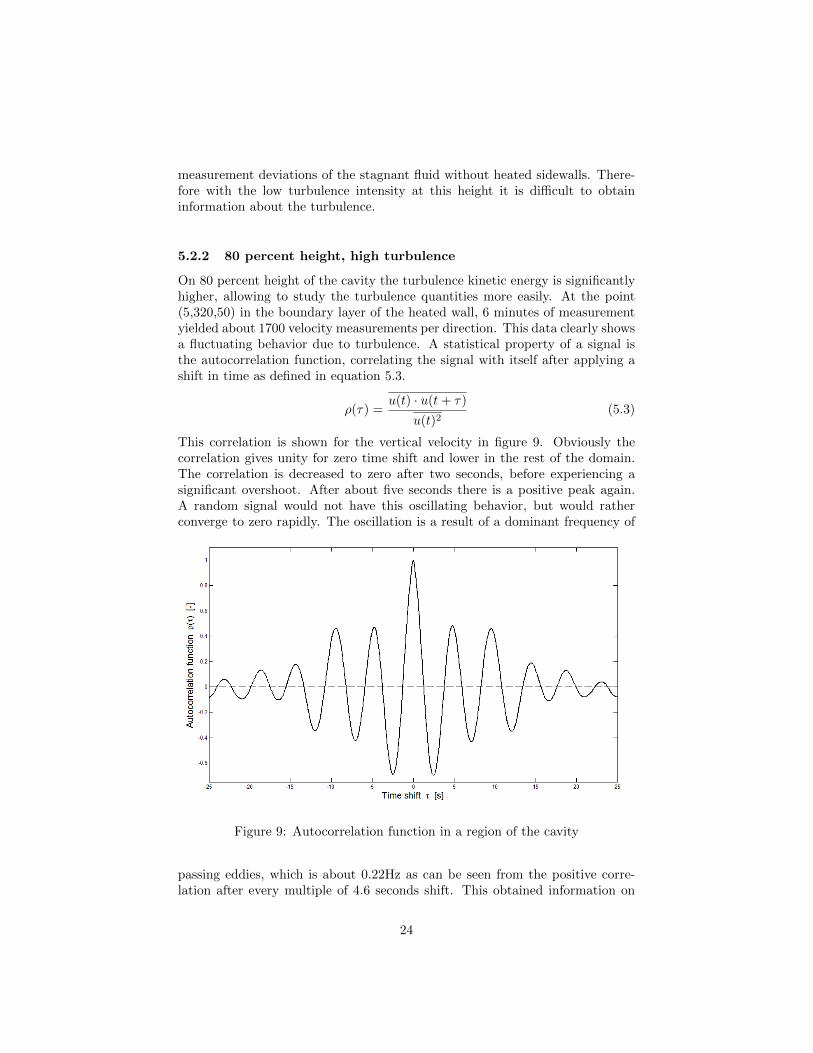
On 80 percent height of the cavity the turbulence kinetic energy is significantlyhigher, allowing to study the turbulence quantities more easily. At the point(5,320,50) in the boundary layer of the heated wall, 6 minutes of measurementyielded about 1700 velocity measurements per direction. This data clearly showsa fluctuating behavior due to turbulence. A statistical property of a signal isthe autocorrelation function, correlating the signal with itself after applying ashift in time as defined in equation 5.3.

ρ(τ) =u(t) · u(t+ τ)

u(t)2(5.3)

This correlation is shown for the vertical velocity in figure 9. Obviously thecorrelation gives unity for zero time shift and lower in the rest of the domain.The correlation is decreased to zero after two seconds, before experiencing asignificant overshoot. After about five seconds there is a positive peak again.A random signal would not have this oscillating behavior, but would ratherconverge to zero rapidly. The oscillation is a result of a dominant frequency of

Figure 9: Autocorrelation function in a region of the cavity

passing eddies, which is about 0.22Hz as can be seen from the positive corre-lation after every multiple of 4.6 seconds shift. This obtained information on

24

Figure 10: Mean velocity profiles at 80% height

the passing frequency of the eddies is important for the time to measure at aspecific point in order to obtain statistically stable data. If measurements spanabout 100 eddies, a single eddy will have negligible influence on the statistics.This suggests that collecting 8 minutes of data at every position would givestatistically stable quantities.

With 500 seconds per point, the boundary layer at 80% height is measuredwith the same settings as was done at 50% of the height. Velocities are onlyused if within a time window of 0.1s a measurement is done on both channels,giving the possibility to correlate the velocity deviations between the two direc-tions in order to find the Reynolds stress. By mistake, the measurements areperformed 7mm from the middle in the z-direction. In figure 11 the turbulencequantities for the two directions are visualized. Although sufficient particlesare captured in the specified time, it does not give a really smooth result. Thequantitative behavior and order of magnitude though are clear. The correlationof the velocity fluctuations between the two directions is low, but it is slightlynegative very near the wall and positive further away from the wall, which seemsto make sense, imagining growing eddies. The turbulence kinetic energy, definedby equation 5.4 is calculated assuming that w′ is the mean of u′ and v′, whichis found to be the global behavior near the wall in the DNS data of the air-filledcavity.

k =1

2

[u′2 + v′2 + w′2

](5.4)

25

Figure 11: Turbulence quantities at 80% height

26

6 Particle Imaging Velocimetry

PIV was carried out more often in the past at POLO. The equipment wasavailable and could pretty much be considered as plug and play. The mainfocus of this part was how to position the camera and laser with respect to thecavity. A special part was designed to attach the laser to the traverse system, sodifferent plane depths can be illuminated with remote controlled traverse. Thecamera will be positioned on a stationary fixture. No further activities werecarried out on PIV during the considered period.

27

7 Liquid Crystal Thermography

Liquid Crystal Thermography is a technique that allows one to measure theinstantaneous temperature distribution in a plane, without disturbing the flow.The setup comprises a carefully selected illumination source, liquid crystal par-ticles that are active in the right range and a sensitive color camera. Thecombination should guarantee clear images with a distinctive color to temper-ature relation. In this chapter the subsequent image processing, conversion totemperatures and the calibration method are considered.

7.1 Camera procurement

In this research the camera, capturing the color distribution from the illumi-nated plane in the cavity, plays a key role in the accuracy of the measurements.In LCT experiments usually CCD (charge-coupled device) cameras are usedbecause of their excellent photosensitivity. As a CCD-chip in principle only reg-isters intensity, optics have to be applied in order to extract information aboutthe color contents. One option is to place a color filter on every single pixel,transmitting only red, green and blue alternately. This way two third of theincoming light is rejected and numerical interpolation has to be applied to re-construct the color information in an RGB array. A more sophisticated methodis to split the incoming light in three parts separated by specific wavelengths.The three components are directed to separate CCD chips, giving the name3CCD to this technology. All incoming light is used and can be projected onRGB format directly, giving a very high resolution. Cameras with one CCDchip are considerably cheaper than its three chips alternative. With a certainbudget roughly the same color resolution can be obtained. However, the singleCCD camera needs an images of at least three times the size with the interpo-lated values that do not supply additional information. This increased imagesize is a disadvantage in post-processing time. These considerations have led tothe decision to purchase a professional 3CCD camera for this research.

7.2 Image filtering

The images obtained with the 3CCD camera have to be processed before theycan be used to calculate the temperature distribution. The images will be some-what granular, because of the non-uniform crystal particle distribution. Therewill be voids, small regions without an illuminated particle, depending on theseeding density. As these dark spots contain no useful information, the colordistribution has to be smoothened before the conversion to temperature. Themain purpose of the image processing is to remove high differences in the colorcomponents of neighboring pixels. There are different approaches to filter outhigh frequency noise. The filtering process is a balance between noise reductionand preservation of the underlying physical behavior.

For the application of LCT image processing, combinations of linear filtershave been applied. For example [10] subsequently applies a Fourier filter, and

28

averaging of a 5x5 window to reduce localized noise further. In order to getback some lost sharpness a high boost image preparation is applied. On theother hand non-linear filters are used for the processing of LCT images [11]with encouraging results. A median filter is applied to a 5x5 window to dras-tically reduce the noise content. A median filter returns the value that dividesthe high and low values in a window. This method is used to avoid corrupt datapoints to influence the other points. Because the voids are dark spots, contain-ing no information about the flow, this would be a good strategy. Moreover themedian filter manages to preserve edges and high gradients. The computationaleffort is somewhat higher, as the values need to be ordered before a value isassigned.

As separate filtering of the color components can give new color combina-tions, advanced median techniques for color images are considered [12]. Themost straightforward method is the classic vector median filter, using either theL1 or L2 norm. The method is very costly in computation time and the gain inaccuracy will be small compared to the median filter applied on the colors sepa-rately. This is because of the smooth nature of the problem, as no independentsudden color changes are expected and therefore no unrealistic new colors willbe generated.

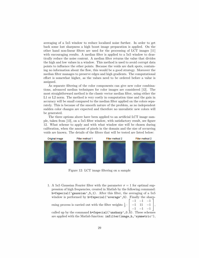
The three options above have been applied to an artificial LCT image sam-ple, taken from [13], on a 5x5 filter window, with satisfactory result, see figure12. What scheme to apply and with what window size will be chosen duringcalibration, when the amount of pixels in the domain and the size of occurringvoids are known. The details of the filters that will be tested are listed below:

Figure 12: LCT image filtering on a sample

1. A 5x5 Gaussian Fourier filter with the parameter σ = 1 for optimal sup-pression of high frequencies, created in Matlab by the following command:h=fspecial(’gaussian’,5,1). After this filter, the averaging of a 5x5window is performed by h=fspecial(’average’,5). Finally the sharp-

ening process is carried out with the filter weights 13 ·

−1 −1 −1−1 11 −1−1 −1 −1

,

called up by the command h=fspecial(’unsharp’,0.5). These schemesare applied with the Matlab function: imfilter(image,h,’symmetric’),

29

where special care is taken with the boundaries by the last entry. ’sym-metric’ mirrors the pixel values in the boundary, so no corrupt data entersthe domain.

2. A median filter applied on a 5x5 window for the color components sep-arately. The command medfilt2(image(:,:,i),[5 5],’symmetric’)

with the index denoting the color component.

3. A vector median filter applied on a 5x5 window: For every point in thewindow the absolute distance in the color space to the other points iscalculated and added up. The middle pixel gets the lowest value of theseL1 norms within the window. The code had to be written manually asMatlab only has a scalar median filter. The computation time is a fewminutes, so for real time processing this filter is not suitable.

4. Identical to 1, with the Gaussian and averaging filters working upon a 7x7window.

5. Identical to 2 applied to a 7x7 window.

6. Identical to 3, but on a 7x7 window.

7.3 Conversion to temperature

Once the images of the liquid crystals are smooth, an attempt can be madeto transfer it to an accurate temperature distribution. As pointed out in [14]the correlation between the color and temperature can be carried out with oneparameter for the color. But by the use of more parameters to describe thecolor, the accuracy and useful range of the spectrum might be increased.

7.3.1 One-parameter correlation

The color of the liquid crystal changes with the temperature, therefore the mostconvenient conversion to find the temperature corresponding to a certain coloris to convert the RGB color components to the HSI space and find a correlationbetween hue and temperature. The conversion from RGB to the hue value iscarried out with [15]:

H =

cos−1(

12 [(R−G)+(R−B)

[(R−G)2+(R−B)(G−B)]1/2

)for B ≤ G

2π − cos−1(

12 [(R−G)+(R−B)

[(R−G)2+(R−B)(G−B)]1/2

)for B > G

(7.1)

By curve fitting a one-to-one relationship between color and temperature is ob-tained.

The correlation between hue and temperature is usually not a simple mono-tonically increasing function. The useful range may therefore be restricted tothe region where the hue is changing enough with temperature. When the slopebecomes too small the error increases to unacceptable values. A reduction in

30

the error and an extension of the useful range might be obtained by combin-ing the hue-temperature relationship with the dependency of temperature onsaturation and/or intensity.

S = 1− min(R,G,B)13 (R+B +G)

(7.2)

I =1

3(R+B +G) (7.3)

For a specific type of crystal liquids, a more monotonically increasing rela-tionship is obtained by correlating the temperature to the hue divided by theintensity [14]. This method requires a combination of the variables that definea color in order to obtain the best correlation with the temperature, which willdepend on the setup configuration and the characteristics of the used liquidcrystal particles.

7.3.2 Neural networks

In the above strategy the three color components of an image are reduced to oneparameter before a one-to-one conversion to the temperature field. Althoughpretty accurate results can be obtained by choosing the right parameter, betterresults can be obtained when no information is thrown away. By using all threecolor parameters in either RGB or HSI space, the error is reduced further andthe useful range is maximized. The relation between the three variable colorinput and the temperature output can be obtained by means of an artificialneural network.

The neural network consists of one or more hidden layers between the inputand output variables. By training the network with input data accompaniedwith the desired output, connections between neurons in the hidden layer will beassigned weights. After enough training the established network can convert thecolor images with high accuracy, given that the training data was a consequentset of data. In literature neural networks with four input parameters are alsoused. Besides the RGB values, also the corresponding hue is used as well [16].As the hue is not independent of RGB, no additional information is providedto the neural network, but it can be seen as an extra weight on this mostmonotonically increasing parameter.

7.4 Calibration

The calibration has to provide the relationship between the color images and thetemperature field. An inaccurate calibration will cause all obtained temperaturefields to be erroneous, therefore this process has to be fulfilled with care. Animportant requirement for calibration is that the circumstances are the same asduring the actual measurements. Although for example calibration with a drysubstrate on a temperature controlled plate might be more accurate, it will nottake into account effects because of dispersion in the fluid and voids between

31

particles which can be expected in the real measurement. For calibration of oursetup there are two viable options for calibration.

1. Instead of applying differential heating, the temperature controlled wallsare kept at the same temperature. When the temperature of the fluidis constant, the color is captured at the depth of the illuminating plane.This procedure is repeated for every tenth of a degree over the activerange of the liquid crystals. The depths of the illuminated plane shouldbe chosen the same as for the measurements as this will influence mainlythe intensity of the received colors. This method will take some time as forevery temperature step it will take time to reach a uniform temperature.Moreover it will yield a limited amount of data points with considerableuncertainty. A spline can be fitted through the filtered and averageddata for the one-parameter correlation. For the neural network a twodimensional filtered color field will give plenty of training data.

2. A second method relies on the physics of heat transport. When a stagnantfluid is subjected to a temperature difference, a constant heat flux and alinear temperature profile will develop. This situation can be obtained inthe cavity if the present body force is eliminated. This is done by tiltingof the cavity, such that the heated wall is on top and the cooled wall thebottom. Buoyancy will play no role in this configuration and a strati-fied temperature distribution will be found. Just one image can providesufficient information for calibration. Most of the uncertainty will be inthe temperatures at the walls, a smooth linear temperature distributionis assumed between these values. A filtered calibration image can be av-eraged over the x-axis, directly yielding a discrete correlation. For theneural network the horizontal lines are training data for one temperature.This method is the convenient choice and will be used if an accurate andreproducible correlation between color and temperature can be obtained.

32

8 Heat Flux

The experiments for obtaining the heat flux at the wall will be the last part ofthe research. Only for this last setup the heated walls will be equipped with heatflux sensors. The sensors are basically a small plate with known thickness andthermal conductivity with thermocouples measuring the temperature differenceat both sides. This data can be converted to heat flux values straightforwardly.During the internship this particular part was not yet considered, only the designand positioning of the heat flux sensors was discussed briefly.

33

9 Conclusions

During the internship period some experience has been gained on numericallysolving a buoyancy driven flow field, with turbulence involved. It is found thatdespite the developments in the field of computational fluid dynamics, obtain-ing a satisfying solution is not at all guaranteed. The combination of turbulentnatural convection close to the wall and a stagnant core region with stratifiedtemperature distribution proves to be a very challenging problem to solve nu-merically. Meshing and the solution strategy have to be adapted to the usedmodel and chosen with care. When the calculation converges to a solution, theresults have to be checked carefully for reasonable behavior.

The difficulties described above call for improved numerical models, espe-cially for turbulent flows. This emphasizes the need for an extensive range ofexperimental data for validation purposes. The experimental data that will beobtained on the differential heated cavity will extend the available data to aregion with higher turbulence intensity.

Preliminary results with LDV measurements show consistent and accurateresults. The velocity profile can be measured up to a quarter of a millimeterclose to the wall. In the region with higher turbulence kinetic energy, the sep-arate eddies can be recognized and the behavior of Reynolds stresses can bedetermined.

PIV and LCT yet have to prove their accuracy and ability in extracting tur-bulent quantities. If the cameras are capable of capturing sharp images of theparticles suspended in the flow at a sufficiently high rate, such data could beextracted. It should be noted that no statistics will be obtained on the correla-tion between temperature and velocity fluctuations, because the techniques willbe applied separately. However, the effect of the turbulence quantities on themean quantities will be captured in this research. Increased transport of heatand dissipation of momentum will be noticed and will be useful for validationpurposes.

9.1 Postscript

This internship period has been a valuable experience. A good insight of theactivities involved in experimental research is obtained, varying from a thoroughunderstanding of the theory and using high end equipment, to solving practicalproblems and cleaning the test section. A lot has been learned on turbulencebehavior and modeling on which I had no prior knowledge. Together with theabroad experience, this has been an internship I’ll never forget.

I would like to thank Cesar Deschamps and Harry Hoeijmakers for makingthis internship possible, especially on such a short notice. Furthermore I wouldlike to thank Andre Popinhak for his guidance and an enjoyable time in thelaboratory.

34

10 Appendix A

Used instrumentation for particle doppler velocimetry:

Instrument Description Model

Laser Water cooled Argon Ion Laser Coherence Innova 70c 2Multicolor beam separator Splits beam and applies phase shift fbl-2 FiberlightFiberoptic Probe Emits beams and collects backscatter TR60 TLN06-363Photodetector box Converts light to electrical signal PDM 1000Signal processor Processes the signal from the PDM FSA 4000Laser Power meter Meter for laser power optimization Coherent FieldMateSeeding particles Reflect light with a Doppler shift Dantec PSP5

35

References

[1] J. Salat, S. Xin, P. Joubert, A. Sergent, F. Penot, and P. Le Quere. Ex-perimental and numerical investigation of turbulent natural convection ina large air-filled cavity. Int. J. of Heat and Fluid Flow, 25:824–832, Apr2004.

[2] W.H. Leong, K.G.T. Hollands, and A.P. Brunger. On a physically-realizable benchmark problem in internal natural convection. Int. J. ofHeat and Fluid Flow, 41:3817–3828, Feb 1998.

[3] M.A.H. Mamun, W.H. Leong, K.G.T. Holland, and D.A. Johnston.Cubical-cavity natural-convection benchmark experiments: an extension.Int. J. of Heat and Fluid Flow, 46:3655–3660, Mar 2003.

[4] Y.S. Tian and T.G. Karayiannis. Low turbulence natural convection in anair filled square cavity. Int. J. of Heat and Fluid Flow, 43:849–884, Jun1999.

[5] F. X. Trias, M. Soria, A. Olivia, and C.D. Perez-Segarra. Direct numeri-cal simulations of two- and three-dimensional turbulent natural convectionflows in a differentially heated cavity of aspect ratio 4. J. Fluid Mech.,586:259–293, Apr 2007.

[6] H.K. Versteeg and W. Malalasekera. An introduction to computational fluiddynamics. Longman scientific & technical, first edition, 1995.

[7] Ansys, inc. Ansys Fluent 12.0 Theory Guide, 12 edition, jan 2009.

[8] Mirko Javurek. Scheme-programmierung in fluent 5&6. unknown, Oct2004.

[9] TR/TM Series Fiberoptic Probes Owner’s Manual, revision b edition, Nov2005.

[10] P.M. Lutjen, D. Mishra, and V. Prasad. Three-dimensional visualizationand measurement of temperature field using liquid crystal scanning ther-mography. J. of Heat Transfer, 123:1006–1014, Oct 2001.

[11] Yu Rao and Shusheng Zang. Calibrations and the measurement uncertaintyof wide-band liquid crystal thermography. Measurement Science and Tech-nology, 21:015105–015112, Nov 2009.

[12] Andreas Koschan and Mongi Abidi. A comparison of median filter tech-niques for noise removal in color images. Proc. 7th German workshop oncolor image processing, 34:69–79, Oct 2001.

[13] N. Fujisawa and Y. Hashizume. An uncertainty analysis of temperature andvelocity measured by a liquid crystal visualization technique. MeasurementScience and Technology, 12:1235–1242, May 2001.

36

[14] N. Fujisawa and R.J. Adrian. Three-dimensional temperature measurementin turbulent thermal convection by extended range scanning liquid crystalthermometry. j. of Visualization, 1:355–364, Feb 1999.

[15] Gonzalez and Woods. Digital Image Processing. Addison-Wesley, firstedition, 1992.

[16] G.S. Grewal, M. Bharara, J.E. Cobb, V.N. Dubey, and D.J. Claremont.A novel approach to thermochromic liquid crystal calibration using neuralnetworks. Measurement Science and Technology, 17:1918–1924, April 2006.

37