A Numerical and Experimental Study of the Dynamics of the … · · 2018-03-27of the Dynamics of...

L3 Internship

A Numerical and Experimental Studyof the Dynamics of the Foucault

Pendulum Subject to PerturbationsThomas Portier & Ridhuan Shukor

April to May 2013

Supervisors :Achim Wirth, Research Fellow at CNRS

Tristan Vandenberghe, Project Engineer at LEGI

Joseph Fourier University, L3 MécaniqueLEGI Laboratory / Team MEIGE

Acknowledgment

We want to give special thanks to Mr. Christophe Baudet, the Director of LEGI Laboratory. Without

his effort, it would be impossible to bring the whole project to the light.

We also express our heart full of gratitude and indebtedness to Mr. Achim Wirth and Mr. Tristan

Vandenberghe for their scholastic guidance, salutable instructions, constructive criticism, and constant

help in carrying out this internship to the very successful completion.

We are also thankful to Mr. Nathanäel Connesson, Mechanics of Materials Professor, Department of

Mechanical Engineering, Joseph Fourier University for consenting to be our supervisor of the Internship

Program.

Our sincere gratitude also goes to our colleagues who helped a lot during our internship, Miss Aimie

Moulin, Miss Sophie Metivier and Mr. Thibault Oudart who contributed in many ways to our internship.

Finally, we would like to express our overall gratitude to all other employees of LEGI Laboratory who

contributed to the project and finally to everyone from our Mechanical Engineering department for the

direct and indirect support through out the year.

Thomas Portier & Ridhuan Shukor

Abstract

The Foucault Pendulum is a well known device in physics world invented in 1851 by Sir Léon Foucault,

a renowned french scientific journalist, in order to demonstrate the theory of the rotation of Earth. This

pendulum exists in museums and universities all around the world to prove the phenomenon of the rotation

of the Earth. While the LEGI Laboratory is in the process of installing its very own Foucault Pendulum, it

is our internship’s subject to make a study of the pendulum at different levels of precisions and hypotheses,

while taking in consideration the studies that have already been made on the subject.

The first part of our internship was devoted to the construction of the mathematical and numerical

models of the pendulum. First we had to build a method of calculation of the pendulum, comprised of

several mathematical models according to the level of approximation. The numerical models were construc-

ted to solve the mathematical models. These numerical models were then integrated into programming

softwares. We used Scilab and Matlab as our programming softwares to build the numerical models and

the visualisation of the pendulum’s movement. The results of the numerical solutions were then compared,

at several orders of precision, with the analytical solutions derived from our mathematical models. In a

bigger scope of study, we take into consideration the existence of external perturbation into the pendulum,

such as the friction, which make an extra case of study of the dynamics of the pendulum.

The second part of our internship was dedicated to the verification and the validation of the numerical

model with the true Foucault Pendulum that was freshly installed in the laboratory.

Contents

1 Introduction 1

1.1 Presentation of the LEGI Laboratory and Team MEIGE . . . . . . . . . . . . . . . . . . . . 1

1.2 Presentation of the internship’s project . . . . . . . . . . . . . . . . . . . . . . . . . . . . . . 2

1.3 Physical problem considered . . . . . . . . . . . . . . . . . . . . . . . . . . . . . . . . . . . . 3

2 Models 4

2.1 Mathematical model . . . . . . . . . . . . . . . . . . . . . . . . . . . . . . . . . . . . . . . . 4

2.1.1 Newtonian method . . . . . . . . . . . . . . . . . . . . . . . . . . . . . . . . . . . . . 4

2.1.2 Analytical solution . . . . . . . . . . . . . . . . . . . . . . . . . . . . . . . . . . . . . 8

2.2 Numerical model . . . . . . . . . . . . . . . . . . . . . . . . . . . . . . . . . . . . . . . . . . 9

2.2.1 The idealised model of the pendulum . . . . . . . . . . . . . . . . . . . . . . . . . . . 9

2.2.2 Evaluation of the pendulum’s trajectory in true and apparent equilibrium position . 11

2.2.3 The real model: Friction, Stokes and Quadratic Drag . . . . . . . . . . . . . . . . . . 12

2.2.4 Runge-Kutta calculation . . . . . . . . . . . . . . . . . . . . . . . . . . . . . . . . . . 15

2.2.5 Difference between numerical and analytical solution . . . . . . . . . . . . . . . . . . 18

2.3 External Perturbation . . . . . . . . . . . . . . . . . . . . . . . . . . . . . . . . . . . . . . . 20

2.3.1 Eccentricity of the plane of the pendulum’s oscillation . . . . . . . . . . . . . . . . . 20

2.4 Deviation of the oscillation’s plane . . . . . . . . . . . . . . . . . . . . . . . . . . . . . . . . 21

3 Experimental results 23

3.1 Objectives . . . . . . . . . . . . . . . . . . . . . . . . . . . . . . . . . . . . . . . . . . . . . . 23

3.2 Procedures . . . . . . . . . . . . . . . . . . . . . . . . . . . . . . . . . . . . . . . . . . . . . 23

3.3 Initial conditions . . . . . . . . . . . . . . . . . . . . . . . . . . . . . . . . . . . . . . . . . . 23

3.4 Results & Analysis . . . . . . . . . . . . . . . . . . . . . . . . . . . . . . . . . . . . . . . . . 24

4 Conclusion 29

4.1 Professional conclusion . . . . . . . . . . . . . . . . . . . . . . . . . . . . . . . . . . . . . . . 29

4.2 Personal conclusion . . . . . . . . . . . . . . . . . . . . . . . . . . . . . . . . . . . . . . . . . 29

4.3 Professional & personal perspective . . . . . . . . . . . . . . . . . . . . . . . . . . . . . . . . 29

A)APPENDIX 1: Numerical model in Scilab i

1 Introduction

1.1 Presentation of the LEGI Laboratory and Team MEIGE

The Laboratory of Geophysical and Industrial Flows / Laboratoire des Ecoulements Géophysiques

et Industriels (LEGI) is a public research laboratory at the University of Grenoble. It is a member of

Joint Research Unit (UMR 5519) at the National Centre for Scientific Research (CNRS), Joseph Fourier

University (UJF) and the National Polytechnic Institute of Grenoble (Grenoble-INP), which employs more

than 180 people, including 70 permanent researchers and many PhD students and postdocs, as well as

intern students. The laboratory is located within the heart of University of Grenoble.

Research activities conducted by the LEGI laboratory are focused on the field of Fluid Mechanics

and Transfers. They rely on a combination of methodological approaches combining modelling, exper-

iments (more than 40 large experimental instruments such as the wind tunnel for low level turbulence,

the hydrodynamics water tunnel, the huge Coriolis turntable and many more), high-performance numer-

ical simulations (which include parallel computing machines and national calculators) and development

of innovative measurement instruments. These activities are related to many application areas within

environmental issues as well as industrial covering the fields of natural environment and decision support,

environmental engineering as well as energy engineering.

Figure 1: From left (a) Coriolis turntable, (b) Hydrodynamics water tunnel, (c) Wind tunnel for low level

turbulence

The main research themes conducted here are:

• The dynamics of turbulent flows (hydrodynamics, mixing, heat transfers etc)

• Geophysical fluid dynamics (simulations of natural processes and systems (ocean, atmosphere, coastal,

river etc), understanding of climate change and development of forecasting tools)

• Flow dynamics in strong hydrodynamic coupling (physical modelling of flow and high density con-

trast, discrete multiphase flows (bubbles, drops))

Here in the LEGI laboratory, there are 4 working teams:

• Team EDT: Multiphase flows and turbulence

• Team Energy

• Team MEIGE: Modeling, Experiments and Instrumentation for Geophysics and Environment

• Team MOST: MOdeling and Simulation of Turbulence

1

For our project, we worked with the Team MEIGE, under the surveillance of Mr. Achim Wirth and

the project engineer Mr. Tristan Vandenberghe.

Team MEIGE

The Team MEIGE (Modeling, Experiments and Instrumentation in Geophysics and Environment)

researches are related closely to the theme of LEGI laboratory: ocean, atmosphere and coastline. The

team is led by Mrs. Chantal Staquet, our own mathematics professor in the university. The studies focus

on the dynamics of these environments at local-scales such as: boundary currents in the ocean or the

braking of surface surface waves on the shore. They seek to understand and model the processes. The

team consists of twelve researchers and academics.

The notable experimental facilities used by the team is the Coriolis turntable having for diameter as

big as 13m, and the newly installed Foucault pendulum which is exactly our subject of internship.

1.2 Presentation of the internship’s project

The Foucault pendulum is, in itself, a clever piece of engineering. It has proven to be a low-cost

demonstration of the rotation of the Earth. The pendulum derived its name from Sir Jean Bernard Léon

Foucault, a french scientific journalist who invented the pendulum in 1851. By his time, the rotation of

the Earth was no longer in dispute, but there was still no direct way to demonstrate or measure it.

Foucault found out that the plane of oscillation of a pendulum is not affected by the twist of its fixed

point. Thus, the pendulum’s plane of oscillation can be used as a fixed plane in order to prove Earth’s

rotation. Foucault reasoned that if he hung a pendulum from a fixed point and the direction of the

pendulum’s swing appeared to change, that could only be because the Earth itself was moving underneath

the pendulum.

Thanks to this simple yet massive discovery, it has become the pioneer into proving the rotation of

the Earth. Nowadays, it is one of the most present mechanical devices in educational institutes as well as

science museums. For this reason, the LEGI laboratory has decided to install one of this pendulums in its

newly-built exhibition hall, which will be opened to all public, scientific students included.

When we arrived in the laboratory, the pendulum was currently being installed. Thus the objective

of our study was to construct a complete model of the Foucault pendulum; from mathematical model, to

numerical model and its visualisation, to experimental results and finally verify the validity of all models

and results. Only then the pendulum will be opened to all public.

2

1.3 Physical problem considered

The pendulum studied is a Foucault pendulum installed in the LEGI laboratory for public access.

Unlike the other simple pendulums, the pendulum that we had to study is specially designed in order to

demonstrate the rotation of the Earth.

For this cause, we will have to determine certain values which will be crucial for our study that follows:

the latitude of the place where the pendulum is suspended (latitude of the LEGI laboratory), the terrestrial

radius, the exact gravitational acceleration of the place the pendulum is suspended, and the properties of

the pendulum itself.

The pendulum’s bob is made of brass, it has a mass of 45kg, its radius counts 0.11m, and the wire’s

length is 7.98 m. The pendulum is suspended in the hall in the heart of the LEGI laboratory. The physical

model is well installed, and it is our goal to construct a comprehensive numerical model which describes

the dynamics of our pendulum.

The Coriolis effect presents a small perturbation (Ω = 6.58 × 10−5 ω =⇒ Ω ω) to the pendulum’s

dynamics. The experiment has to be performed with special cave to avoid other type of perturbations

which can potentially masque the Coriolis effect.

Figure 2: The pendulum’s bob, weighs 45 kg

3

2 Models

2.1 Mathematical model

First of all, from the physical model we will proceed with the construction of the mathematical model.

2.1.1 Newtonian method

Figure 3: Terrestial spherical frame of reference

Let us adopt the frame of reference conventions represented in fig. (3). Consider the figure illustrated

below, ϕ defines the latitude of the place where the pendulum is suspended, the sets of vectors (UrUϕ, UyUz)

(refer fig. (3)) are superposed and the two planes built from those vectors are coplanar, therefore one can

translate the set of vector (UrUϕ) to the Earth’s center to have the plane illustrated as below:

Figure 4: Plane showing the projection of Earth’s rotational vector onto the local frame of reference

The Earth is rotating about the axis −→Uz, to study the pendulum’s dynamics in local scale, one has to

project the Earth’s rotation onto the local frame of reference, from fig. (4) the Earth’s rotational vector

can therefore be expressed as:−→Uz = sinϕ

−→Ur + cosϕ

−→Uϕ (1)

4

As a result, the Earth’s rotational vector −→Ω will be expressed as such in the local frame of study:0

0

Ω

(x,y,z)

=

Ω sinϕ

0

Ω cosϕ

(r,θ,ϕ)

(2)

The following figure illustrates the local frame of reference in which the pendulum swings and where

our study will be focused on:

Figure 5: Local frame of reference of the pendulum

From fig. (5), one uses Chasles’ relation to express the pointM , the position of the bob at instantaneous

moment, R is the projection of the point M on the axis −→Ur, r = (the Earth’s radius + ‖−−→OR‖), x and y are

the positions in projection to respective vectors:

−−→OM =

−−→OR+

−−→RM (3)

= r−→Ur + x

−→Uθ + y

−→Uϕ (4)

The velocity of the bob is given by:

−→V (−−→OM)R =

d(−−→OM)

dt(R)=

d

dt(R)(r−→Ur + x

−→Uθ + y

−→Uϕ) (5)

= r−→Ur + r

d−→Ur

dt(R)+ x−→Uθ + x

d−→Uθ

dt(R)+ y−→Uϕ + y

d−→Uϕ

dt(R)(6)

Since the vectors −→Ur,−→Uθ and

−→Uϕ are the vectors of a non-inertial frame of reference, the time derivatives

of those vectors depend on the inertial frame of reference. In our study, assume the Earth to be immobile,

therefore Earth is the inertial frame of reference. The time derivative is expressed:

d−→Ui

dt(R)=

d−→Ui

dt(R′)+−→Ω (R′/R) ×

−→Ui (7)

5

where −→Ui is the position vector of the pendulum, R is the terrestrial frame of reference and R′ is the local

frame of reference. Since there is no acceleration of the local frame of reference with respect to its own

reference, one has:d−→Ui

dt(R′)= 0 (8)

Hence the derivative of the local plane’s vectors with respect to time is expressed by using the eq. (7):

d−→Ur

dt(R)=

d−→Ur

dt(R′)+

Ω sinϕ

0

Ω cosϕ

(r,θ,ϕ)

×

Ur

0

0

(r,θ,ϕ)

=

0

Ω cosϕ

0

(r,θ,ϕ)

(9)

d−→Uθ

dt(R)=

d−→Uθ

dt(R′)+

Ω sinϕ

0

Ω cosϕ

(r,θ,ϕ)

×

0

Uθ

0

(r,θ,ϕ)

=

−Ω cosϕ

0

Ω sinϕ

(r,θ,ϕ)

(10)

d−→Uϕ

dt(R)=

d−→Uϕ

dt(R′)+

Ω sinϕ

0

Ω cosϕ

(r,θ,ϕ)

×

0

0

Uϕ

(r,θ,ϕ)

=

0

−Ω sinϕ

0

(r,θ,ϕ)

(11)

with Ur, Uθ and Uϕ are the unit vectors.

On account of the negligible effect of the variation in r with respect to the pendulum’s length and

oscillation, one can consider a case study of the plane movement:

dr

dt(R)= r = 0 (12)

The velocity of the bob is given by:

−→V (−−→OM)R = 0 + rΩ cosϕ

−→Uθ + x

−→Uθ + xΩ(sinϕ

−→Uϕ − cosϕ

−→Ur) + y

−→Uϕ

−yΩ sinϕ−→U (13)

= (−xΩ cosϕ )−→Ur + (x+ rΩ cosϕ − yΩ sinϕ )

−→Uθ + (xΩ sinϕ + y)

−→Uϕ (14)

Before proceeding with the acceleration, one introduces the constants ϕ = 0 Pendulum’s latitude is constant

Ω = 0 Earth’s rotational speed is constant(15)

Due to these terms equal to zero, the final expression of the bob’s acceleration can be simplified, and

therefore expressed as such:

−→Γ (−−→OM) =

d−→V (−−→OM)

dt(R)(16)

= (−xΩ cosϕ )−→Ur + (−xΩ cosϕ )(Ω cosϕ

−→Uθ) + (x− yΩ sinϕ )

−→Uθ)

+(x+ rΩ cosϕ − yΩ sinϕ )(Ω sinϕ−→Uϕ − Ω cosϕ

−→Ur) + (xΩ sinϕ + y)

−→Uϕ

+(xΩ sinϕ + y)(−Ω sinϕ−→Uθ) (17)

= (x− 2yΩ sinϕ − xΩ2)−→Uθ + (y + 2xΩ sinϕ − yΩ2 sin2 ϕ

+rΩ2 cosϕ sinϕ )−→Uϕ (18)

6

Let us introduce the forces acting on the pendulum’s bob: the bob’s weight P itself, and the wire’s

tension T . Consider the fig. (5), the net force is given in the following expression, one can eventually

project the force vectors onto the vectors that are parallel and orthogonal to the pendulum’s movement,

where α is the instantaneous angle of the pendulum’s movement:∑(−−−−→F ext/b) =

−→T +

−→P (19)

= T−→Ut − P

−→Ur (20)

= T−→Ut − P cosα

−→Ut + P sinα

−→Ua (21)

The projection onto −→Ut gives:

T − P cosα = 0 (22)

Hence the only term of the net force acting on the bob is P sinα−→Ua. Assume the projection of the net

force onto the vector −→Uθ and −→Uϕ, where P = mg, m the mass of the bob, g the gravitational acceleration

of the place the pendulum is suspended, M the instantaneous position of the bob, R the projection of the

point M to the axis −→Ur, l the length of the pendulum’s wire:∑(−−−−−→F ext/b) = mg sinα

−→Ua (23)

= mg(RM

l)−→Ua (24)

=mg

l(x−→Uθ + y

−→Uϕ) (25)

Now that all the necessary terms have been calculated, let us introduce the Newton’s second law of

motion in order to express the equations of the pendulum’s dynamics:∑(−−−−−→F ext/b) = m

−→Γ (26)

From the previous calculations, one can simply rewrite the Newton’s second law of motion as such:

mg

l(x−→Uθ + y

−→Uϕ) = mΓ

−→Ua (27)

The term√

gl = ω0 which represents the pendulum’s period is introduced to simplify the expression,

one replaces the expression Γ by its expression described in eq. (18):

mω20(x−→Uθ + y

−→Uϕ) = m(x− 2Ω sinϕ y − xΩ2)

−→Uθ

+m(y + 2Ω sinϕ x− yΩ2 sin2 ϕ + rΩ2 cosϕ sinϕ )−→Uϕ (28)

For a more simplified expression, let us project the acceleration on their respective vectors:

−→Uθ : x− 2yΩ sinϕ− xΩ2 = ω2

0x (29)−→Uϕ : y + 2xΩ sinϕ− yΩ2 sin2 ϕ+ rΩ2 cosϕ sinϕ = −ω2

0y (30)

Finally the equations of the pendulum’s dynamics is expressed as below, one ignores the terms xΩ2

and yΩ2 sin2 ϕ because with the value of order 10−10m.s−2, they have a negligible effect with respect to

other terms of the equations.

x− 2Ω sinϕ y + ω20x = 0 (31)

y + 2Ω sinϕ x+ ω20y = −rΩ2 cosϕ sinϕ (32)

7

2.1.2 Analytical solution

In the laboratory’s frame of reference, the point of suspension of the pendulum lies at altitude l =

7.98 ± 0.005m, (the Earth’s radius + laboratory’s altitude) r = 6.371397 × 106m, the Earth’s angular

rotational speed Ω = 7.2921150 × 10−5 rad/s, latitude of the laboratory ϕ = 0.788714289 rad, and

gravitational acceleration at the laboratory g = 9.804ms−2.

To solve analytically, assume a system of linear homogenous differential equations:

x0 − 2Ω sinϕ y0 + ω20x0 = 0 (33)

y0 + 2Ω sinϕ x0 + ω20y0 = 0 (34)

Let us introduce the complex variable z0 = x0 + iy0. Multiply the Equation (34) by i and add the

Equation (33), the auxiliary variable z occurs naturally in the unique differential equation:

z0 + 2iΩ sinϕ z0 + ω20 z0 = 0 (35)

To solve the differential equation, one poses the characteristic equation and finds the solution for r:

r2 + 2iΩ sinϕ r + ω20 = 0 (36)

=⇒ r1,2 = −iΩ sinϕ± i√

Ω2 sin2 ϕ+ ω20 (37)

The solution for z is well-known, and expressed in the form of:

z0(t) = C1 er1t + C2 e

r2t (38)

with C1 and C2 the coefficients which depend on the initial conditions (the position and velocity).

One can easily determine the two coefficients by using the matrices. This requires one to derivate the

expression z with respect to time.

z0(t) = C1r1 er1t + C2r2 e

r2t (39)

For initial conditions (t = 0), the matrices are expressed as

A · C = B (40) 1 1

r1 r2

· C1

C2

=

z0(t)

z0(t)

(41)

By using the matrix inversion C = A−1 ·B, the constants C1 and C2 are expressed:

C1 =1

2+

Ω sinϕ√Ω2 sin2 ϕ+ ω2

0

(42)

C2 =1

2− Ω sinϕ√

Ω2 sin2 ϕ+ ω20

(43)

The values of C1 and C2 being replaced in the eq. (38), one can finally obtain the x-position and

y-position by extracting its real part and the imaginary part respectively.

Let us insert the second member of the eq. (32). The equations make a system of non-homogenous

differential equations, which is the system of equations that we try to solve:

x− 2Ω sinϕ y + ω20x = 0 (44)

y + 2Ω sinϕ x+ ω20y = −rΩ2 cosϕ sinϕ (45)

8

To solve the non-homogenous differential equations, consider the equilibrium of the pendulum: x = x = 0

y = y = 0=⇒

x = xeq = constant

y = yeq = constant(46)

Therefore eq. (44) and (45) give:

xeqω20 = 0 (47)

yeqω20 = −rΩ2 cosϕ sinϕ (48)

the true equilibrium position is given by:

xeq = 0 (49)

yeq =−rΩ2 cosϕ sinϕ

ω20

=−rΩ2 cosϕ sinϕ l

2g=−rΩ2 sin(2ϕ) l

2g= −3.752727× 10−4m (50)

The set xeq, yeq is a solution of equations of motion; indeed this is the equilibrium solution. Thus at

equilibrium, the pendulum is not oriented along the true vertical, but along the apparent vertical, which

makes an angle

α ≈ sinα =yeql

=−rΩ2 sin 2ϕ

2g= 0.00269442914 (51)

The term yeq is a particular solution of the non-homogenous equation which gives:

z(t) = C1 er1t + C2 e

r2t + i yeq (52)

Note that from the first stage of analytical calculation, we have made the assumption that the variation

in r is insignificant against the length of the pendulum thus we ignore the term r from the calculation and

the numerical modelling of the pendulum’s swing.

2.2 Numerical model

2.2.1 The idealised model of the pendulum

In a first approximation, an idealised model is constructed to illustrate the pendulum’s movement over

time in its optimum situation. In reality, which is the objective of the internship, the pendulum is subject

to the air resistance and friction, where the pendulum’s amplitude decreases over time.

When set into motion, an idealised pendulum never loses energy to its surroundings. So when released,

and left to swing, the potential energy is converted into kinetic energy and therefore the pendulum swings.

When it reaches its highest point the energy is fully converted back to potential, and as it falls back to

kinetic. As it is "idealised" it never loses energy to friction. Therefore, the conversion of kinetic energy

to potential will always be periodic and it will never stop. Although in reality it is impossible to have an

idealised pendulum, near idealised ones can be obtained by suspending the pendulum in a vacuum.

For the modelling of the idealised model, consider the pendulum’s dynamics where the equilibrium

position is described in true vertical:

x− 2Ω sinϕ y + ω20x = 0 (53)

y + 2Ω sinϕ x+ ω20y = 0 (54)

9

The coupled differential equations described above will be discretised using the Runge-Kutta method, a

numerical method used to solve the problem of differential equations. More details on how to integrate the

differential equations by the Runge-Kutta method will be explained later in the subchapter RK calculation.

The pendulum’s dynamics translated into RK is then programmed in Matlab in order to visualise the

pendulum’s movement. All of the figures and results from this study are obtained from Matlab. Let us

evaluate the oscillation of the pendulum over time, projected onto the axes Uθ and Uϕ, as well as plane

view of the pendulum’s position after a given time.

Figure 6: The rotation of the plane of pendulum’s oscillation after 2 hours

Figure 7: The pendulum’s oscillation in x-position and y-position in 24 hours in the laboratory

From fig. (6), one can see that the plane of the pendulum’s oscillation rotates over time. An explanation

to this, the plane of the pendulum’s oscillation actually remains fixed relative to the distant masses of the

universe while Earth rotates underneath it. So, relative to Earth, the plane of the pendulum’s oscillation

10

suspended in our laboratory supposedly undergoes a full clockwise rotation during one day. However it is

only true at the North and South Pole. As the latitude decreases, the plane of oscillation precesses slower;

and its angular speed $ is proportional to the sine of the latitude ϕ:

$ =360 sinϕ

day(55)

For the latitude of the laboratory ϕ = 45.19, the pendulum will make a rotation of 255.40/day. That

means, in order to make a full 360 rotation, the pendulum will take a total time of 33 hours 49 minutes

and 44 seconds.

This phenomenon can be further explained by studying the fig. (7). In this figure, we set at the

initial launch, the initial conditions of position x=1, position y=0; and the result obtained shows that the

oscillation alternates between the x-axis and y-axis. During a day, we can see that the oscillation with

respect to x-axis decreases while the one with respect to y-axis gains value, vice verca. The figure also

shows the incomplete alternate oscillation after one day; because to make a full rotation, the pendulum

has to come to its initial position, which is not the case in the figure above.

2.2.2 Evaluation of the pendulum’s trajectory in true and apparent equilibrium position

Due to the Earth’s rotation, in the equilibrium position, the pendulum’s bob is not situated exactly

at the point of origin but at the position xeq, yeq as described in the eq. (49) and (50) which we call an

original equilibrium position, and oriented along an apparent vertical.

To evaluate this, we draw a graph with both equilibrium positions oriented along true and apparent

vertical superposed: the system of equations along the apparent vertical is given by eq. (44) and (45),

while the one along the true vertical is given by eq. (53) and (54).

Figure 8: The difference of oscillation of the pendulum after 8000 seconds

11

Figure 9: The close-up trajectories between 2 equilibrium initial positions

The 2 equilibrium positions give a constant interval difference of 0.5% over time. Nevertheless, the

trajectory with the true equilibrium position is not symmetry with respect to the axis UθUϕ. Hence it is

uninteresting to proceed with the true equilibrium position.

For the studies and calculations that follow, we will consider the new equilibrium position x0 = 0, y0 = 0.

2.2.3 The real model: Friction, Stokes and Quadratic Drag

The idealised model of the pendulum is a simulation done in a vacuum and thus, no air resistance. For

anything that has real-world applications, air resistance is an important factor and needs to be taken into

account.

Figure 10: Von Kármán Street (ref: http://panoramix.ift.uni.wroc.pl)

The well known phenomena caused by air friction is the development of the Von Kármán vortex street

trailing the movement of the pendulum. It is caused by the unsteady separation of flow of the air around the

bob as it swings. Nevertheless this vortex street will only form beyond the value of the Reynolds number

RE that causes the instability. The Reynolds number is proportional to the velocity of the pendulum’s

12

bob:

RE =2 vaρR

µ(56)

where va the velocity of the bob, ρ = 1.189 kg.m−3 the density of the air, R = 0.11m the radius of the

bob, µ = 1.983× 10−5N.s.m−2 the dynamic viscosity of the air at temperature T = 25.

From the Matlab data, during 99.9% of the swing’s time, the velocity of the bob gives a Reynolds

number that results in the turbulent flow. The maximum velocity va(max) = 1.173m.s−1 gives the

Reynolds number RE = 15482. Hence the Von Kármán vortex street and the turbulence exist.

Let us analyse the form of the Von Kármán vortex street. From its form, one can assume that the

vortex street leads to a periodic perturbation to our pendulum. Depending on the type of the air flow

around our bob, the bob will undergo two different types of air friction.

The first one is called Stokes’ Drag Fd (inN), a frictional force that is proportional to the velocity of

the bob:

Fd = 6π µR va (57)

Since Stokes’ Drag is proportional to the velocity va of the bob, it has the greatest effect at the launch

of the experiment where the velocity is the greatest. However, the effect of this air friction will only be

visible after a certain time. Stokes’ Drag is dominant in the case of laminar flow. Let us incorporate this

term of Stokes’ Drag into our equations of the pendulum’s dynamics:

x− 2Ω sinϕ y +6πµR

mx+ ω2

0x = 0 (58)

y + 2Ω sinϕ x+6πµR

my + ω2

0y = 0 (59)

It is also interesting to introduce the coefficient friction time FT−1 (in s−1) situated in the eq. (58) and

(59). FT−1 shows the rate of the movement’s decay in which the movement starts to lose its inertia due

to the air resistance.

FT−1 =

6πµR

m= 9.136× 10−7s−1 (60)

The second type of air friction acting on the pendulum’s bob is called quadratic drag FD. The equation

is expressed:

FD =1

2ρCD πR

2 |va| va (61)

where CD is called the drag coefficient (it is a dimensionless number). To determine CD let us introduce a

graph obtained from NASA (ref: http://www.grc.nasa.gov/) that shows the relation between CD and the

Reynolds number.

13

Figure 11: Drag coefficient CD of a sphere as a function of Reynolds number

Since the velocity of the bob is always changing over time of oscillation, and since 99.9% of the time

of oscillation gives turbulent flow, the value of RE(max) = 15500 is chosen as reference for the CD. From

the fig. (11), one has CD ≈ 0.47. The pendulum’s dynamics is now written as:

x− 2Ω sinϕ y +1

2mρCDπR

2|x|x+ ω20x = 0 (62)

y + 2Ω sinϕ x+1

2mρCDπR

2|y|y + ω20y = 0 (63)

Quadratic drag FD is a frictional force that is dominant in the case of turbulent flow. As stated above,

because 99.9% of the time of oscillation gives turbulent flow, the eq. (62) and (63) will be used to study

the dynamics of the Foucault pendulum in the presence of air friction.

The figures that follow illustrate the movement of the pendulum in the horizontal plane for each case

of friction:

Figure 12: Pendulum’s positions for 3 cases of oscillation

14

Figure 13: Pendulum’s oscillation for 3 cases of oscillation

Figure 14: The rotation of the oscillation’s plane for 3 cases of oscillation

From these figures, it is obvious that the quadratic friction is dominant to the dynamics of our pendu-

lum. Hence the eq. (62) and (63) are considered the equations of the pendulum’s dynamics in the presence

of air friction.

2.2.4 Runge-Kutta calculation

The numerical analysis is a powerful method to determine approximate but accurate solutions to the

complex ordinary differential equations. Runge-Kutta (RK) method are among the most popular ODE

solvers used in numerical analysis. There are many other methods of numerical computation, but for our

study we chose the RK method which we are most familiar with. The origin of the RK method comes

15

from the Euler method:

Yn+1 = Yn + dt · f(Yn) (64)

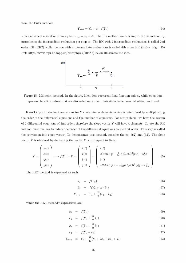
which advances a solution from xn to xn+a = xn + dt. The RK method however improves this method by

introducing the intermediate evaluation per step dt. The RK with 2 intermediate evaluations is called 2nd

order RK (RK2) while the one with 4 intermediate evaluations is called 4th order RK (RK4). Fig. (15)

(ref: http://www.mpi-hd.mpg.de/astrophysik/HEA/) below illustrates the idea.

Figure 15: Midpoint method. In the figure, filled dots represent final function values, while open dots

represent function values that are discarded once their derivatives have been calculated and used.

It works by introducing the state vector Y containing n elements, which is determined by multiplicating

the order of the differential equations and the number of equations. For our problem, we have the system

of 2 differential equations of 2nd order, therefore the slope vector Y will have 4 elements. To use the RK

method, first one has to reduce the order of the differential equations to the first order. This step is called

the conversion into slope vector. To demonstrate this method, consider the eq. (62) and (63). The slope

vector Y is obtained by derivating the vector Y with respect to time.

Y =

x(t)

x(t)

y(t)

y(t)

=⇒ f(Y ) = Y =

x(t)

x(t)

y(t)

y(t)

=

x(t)

2Ω sinϕ y − 12mρCDπR

2|x|x− ω20x

y(t)

−2Ω sinϕ x− 12mρCDπR

2|y|y − ω20y

(65)

The RK2 method is expressed as such:

k1 = f(Yn) (66)

k2 = f(Yn + dt · k1) (67)

Yn+1 = Yn +dt

2(k1 + k2) (68)

While the RK4 method’s expressions are:

k1 = f(Yn) (69)

k2 = f(Yn +dt

2k1) (70)

k3 = f(Yn +dt

2k2) (71)

k4 = f(Yn + k3) (72)

Yn+1 = Yn +dt

6(k1 + 2k2 + 2k3 + k4) (73)

16

Ultimately, the solution for the position and velocity in the axes Uθ and Uϕ is the expression of Yn+1

from the eq. (68) and (73). This solution advances by a step dt until a final given time to describe the

trajectory and the velocity of the pendulum’s bob over time.

Since RK4 method requires twice as much evaluations of the righthand side per step dt as the RK2

method, one might assume the result’s accuracy to be superior to the RK2 by at least twice as large for

the same step. We will compare the 2 methods by calculating the error committed from each method with

the analytical solution from eq. (38). In order to evaluate the error, several steps dt are chosen to plot the

graph: dt = 0.1 s; 0.05 s; 0.025 s and 0.0125 s. The position of the pendulum according to the axis Uθ after

t = 1000s is given in the table (1) below for the calculation using RK2 and RK4 as well as the absolute

error with respect to the analytical solution.

dt(s) RK4 (m) error RK4/analytic (m) RK2 (m) error RK2/analytic (m)

0.1 −0.712967 0.001059 −0.102397 0.611629

0.05 −0.713964 6.274516× 10−5 −1.000513 0.286486

0.025 −0.714023 3.044567× 10−6 −0.807875 0.093848

0.0125 −0.714027 6.028162× 10−7 −0.738590 0.024564

Table 1: The error’s magnitude between RK2 and RK4

The results from the table above is illustrated in the fig. (16) below in logarithm scale.

Figure 16: Error of RK with respect to their steps in logarithm scale.

Firstly, one can easily calculate the slope of each graph and in fact the slope corresponds to the value of

the order of RK method. This means that the RK4 and RK2 have both a slope valuing 4 and 2 respectively.

Secondly, the graphs being plotted in logarithm scale, it is obvious from the graph that RK2 commits an

error that constantly values at twice the error of RK4 with respect to the value of step dt.

17

For this reason, the RK4 is concluded 200% more accurate, hence will be the base of calculation for all

the numerical analysis in our study.

2.2.5 Difference between numerical and analytical solution

In the last subchapter, we have introduced the notion of error between RK method and analytical

solution. In this chapter, we will focus on elaborating the influence and importance of the numerical

solution on the final results with respect to the analytical solution.

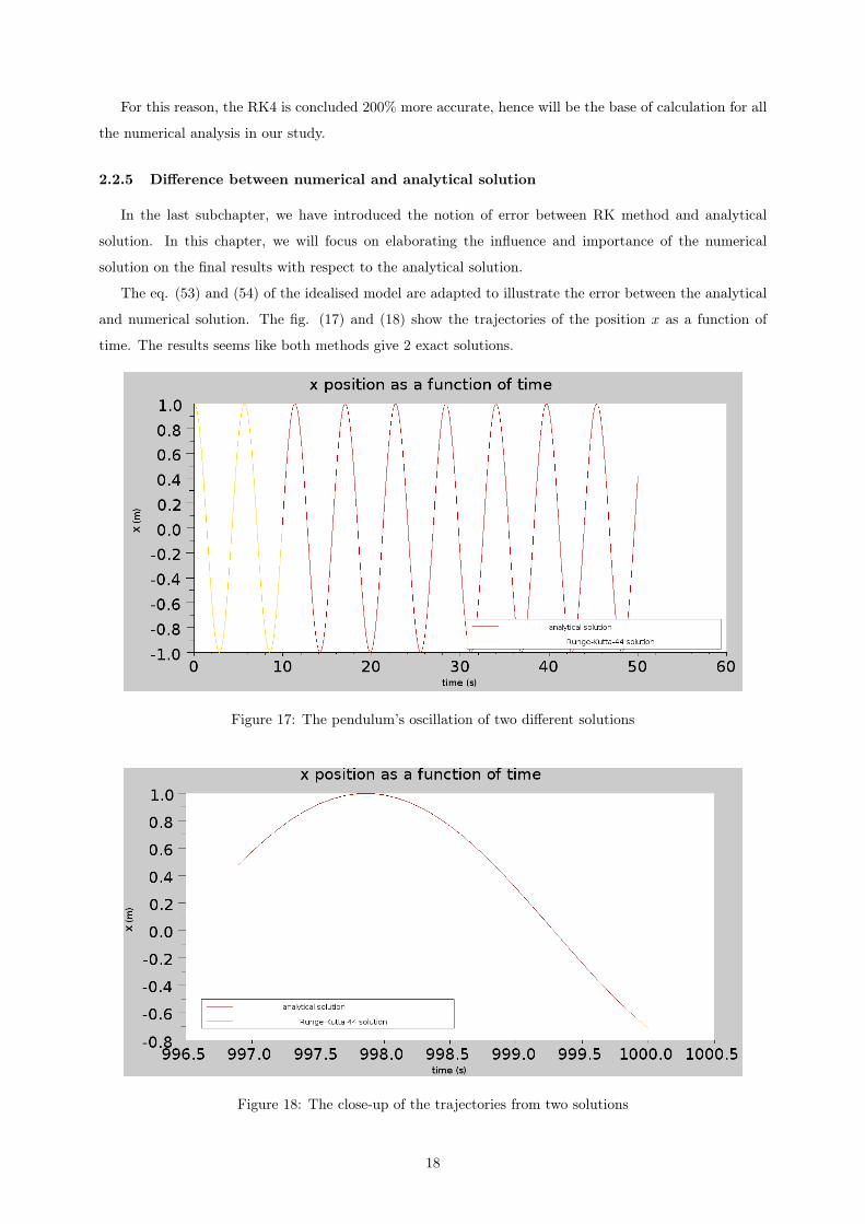
The eq. (53) and (54) of the idealised model are adapted to illustrate the error between the analytical

and numerical solution. The fig. (17) and (18) show the trajectories of the position x as a function of

time. The results seems like both methods give 2 exact solutions.

Figure 17: The pendulum’s oscillation of two different solutions

Figure 18: The close-up of the trajectories from two solutions

18

Nevertheless, let us evaluate the difference of value at every point of the trajectory by calculating the

absolute error of the numerical solution with respect to the analytical solution. The expression of the

absolute error is given by

Absolute error (t) = | Numerical solution (t) - Analytical solution (t) | (74)

Let us plot the graph of absolute error between the numerical solution and analytical solution.

Figure 19: Absolute error between analytical solution and numerical solution

Figure 20: The close-up of the absolute error at the launch of oscillation

From the graphs (19) and (20) above, the error committed by the numerical solution with respect to

the analytical solution increases over time. It is important to note that from fig. (19) the absolute error

increases periodically along the maximum value that appears like a straight line. However after the close

up from fig. (20), one can conclude that the absolute error is periodic and it is synchronised with the

amplitude of the pendulum’s bob itself.

It may seem irrelevant to proceed with numerical study when we register such a growth in absolute

error over time. However, in reality, such visible error will not take place before the pendulum’s oscillation

is greatly reduced by the presence of the air friction. More importantly, the quadratic drag has a non linear

expression, thus when incorporated into the equation of the pendulum’s dynamics, it makes a system of

non-linear differential equation, which is very complicated to solve. By using the numerical method, not

only the calculation is greatly simplified, but the accuracy and the reliability of the results are also hard

to argue.

19

2.3 External Perturbation

In a greater scope of study, consider an external perturbation PE acting upon the pendulum’s bob

apart from the air friction. An example for this is a spontaneous gush of wind coming from outside the

exhibition hall.

Prior to our internship, an observation on this kind of pendulum has been made and it was recorded

that due to the external perturbation, the pendulum’s trajectory takes form of an ellipse rather than a

perfect straight line. Assume the expression of the perturbation is periodic and expressed as:

PE = ε cos(ωpt) (75)

where ωp the period of the perturbation, and ε the perturbation constant, supposedly small in value.

Perturbation’s nature is a force. Its existence will have the influence on the dynamics of the pendulum;

either it adds up the acceleration of the existent movement of the pendulum or slows it down. Depending

on the source of perturbation and the position of the oscillation’s plane, the perturbation will have two

cases of effect: longitudinal and transversal perturbations.

The initial differential equations of movement will take a new form in every case:

•Longitudinal perturbation

x− 2Ω sinϕ y − ε cos(ωpt) x+1

2mρCDAx|x|+ ω2

0x = 0 (76)

y + 2Ω sinϕ x− ε cos(ωpt) y +1

2mρCDAy|y|+ ω2

0y = 0 (77)

•Transversal perturbation

x− (2Ω sinϕ − ε cos(ωpt)) y +1

2mρCDAx|x|+ ω2

0x = 0 (78)

y + (2Ω sinϕ − ε cos(ωpt)) x+1

2mρCDAy|y|+ ω2

0y = 0 (79)

One should take note that the expression of the quadratic drag FD is also already incorporated in the

equation of the pendulum’s dynamics stated above. Hence, the eq. (76), (77), (78) and (79) are the

complete equations for our study, taking in account all the external influences.

2.3.1 Eccentricity of the plane of the pendulum’s oscillation

To characterise the perturbation, the notion eccentricity E of the ellipse is introduced. It is given by

the following relation:

E =

√a2 − b2a2

(80)

where a is the semi-major axis (also the amplitude of the oscillation) and b is the semi-minor axis. This

relation leads to particular cases:E = 0 a perfect circle

0 < E < 1 describes an ellipse

E = 1 a straight line

Let us plot the eccentricity of the oscillation as a function of time.

20

Figure 21: The eccentricity as a function of time

Figure 22: The close up view of the eccentricity

The graphs (21) and (22) above illustrate the evolution of the eccentricity of the pendulum over time

up to 3.5 days.

First it appears that the eccentricity decreases steadily with the existence of the beat phenomenon. The

variation of the eccentricity can be explained by the fact that the amplitude of the oscillation is decreasing

over time due to the air friction while the perturbation is constant, which allow the ellipse to grow while

the amplitude decreases.

The parameters of PE : ωp does not affect E, which is expected since it will actually only affect the

period of the perturbation. On the contrary, E is mostly changed by the variation of the perturbation

constant ε. For example, ε = 10−2 gives E ≈ 1 while ε = 10−1 gives E that is far from a straight line.

2.4 Deviation of the oscillation’s plane

The Foucault pendulum was invented to demonstrate the Earth’s rotation. This was done by showing

that the oscillation’s plane rotates relatively to the Earth. This subchapter will be dedicated to explain

the deviation of the oscillation’s plane over time.

21

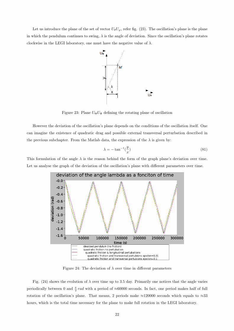
Let us introduce the plane of the set of vector UθUϕ, refer fig. (23). The oscillation’s plane is the plane

in which the pendulum continues to swing, λ is the angle of deviation. Since the oscillation’s plane rotates

clockwise in the LEGI laboratory, one must have the negative value of λ.

Figure 23: Plane UΘUΦ defining the rotating plane of oscillation

However the deviation of the oscillation’s plane depends on the conditions of the oscillation itself. One

can imagine the existence of quadratic drag and possible external transversal perturbation described in

the previous subchapter. From the Matlab data, the expression of the λ is given by:

λ = − tan−1(y

x) (81)

This formulation of the angle λ is the reason behind the form of the graph plane’s deviation over time.

Let us analyse the graph of the deviation of the oscillation’s plane with different parameters over time.

Figure 24: The deviation of λ over time in different parameters

Fig. (24) shows the evolution of λ over time up to 3.5 day. Primarily one notices that the angle varies

periodically between 0 and π2 rad with a period of ≈60000 seconds. In fact, one period makes half of full

rotation of the oscillation’s plane. That means, 2 periods make ≈120000 seconds which equals to ≈33

hours, which is the total time necessary for the plane to make full rotation in the LEGI laboratory.

22

The graph is linear for the idealised pendulum, on the other cases the graphs seem to have slight curve

due to air friction that results in the modified oscillation of the pendulum. It can also be noticed that

the deviation is unaffected by the changes of the parameters ωp. Finally, notice that while comparing the

different conditions of oscillation, the idealised model is in the lead with respect to the real model with

the air friction. Theoretically, in all conditions, the deviation of the oscillation’s plane must be in sync.

3 Experimental results

Our internship was dedicated mostly to the numerical analysis because the pendulum was installed and

ready to be tested only during our last week of internship. Therefore we were not able to experiment and

validate all the numerical analysis that had been done in Matlab.

3.1 Objectives

The objective of the experiment was to validate the numerical and analytical parameters of the pen-

dulum’s dynamics. The experimental parameters observed were:

• The period of oscillation

• The amplitude of oscillation over time

• The semi-minor axis of the oscillation over time

• The deviation of the oscillation’s plane over time

3.2 Procedures

Firstly, since the base measurement scale was not yet installed, it was crucial to position the oscillation

plane correctly which let identifying the parameters during experiments a simple process. The initial launch

of the pendulum is critical; the use of a flame is employed to burn through a thread which temporarily

holds the bob in its starting position, thus avoiding unwanted sideways motion.

Decisive factors:

• The pendulum was suspended at its highest point to a beam (refer fig. (30)) oriented in a particular

direction having for angular orientation 15 or more with respect to the horizontal. Therefore different

angular initial launches will result in completely different trajectory of the pendulum.

• The thread holding the bob was made of different thicknesses and types to test their ability to reduce

the micro vibration during the burning.

• The barrier surrounding the pendulum was not blocked at its bottom-most point, leaving a possibility

for the external air flow to create the perturbation to the pendulum’s oscillation.

3.3 Initial conditions

Experiment 1: Launch at random direction with significant vibration during launching.

Experiment 2: Perpendicular launch to the supporting beam with a little vibration at launching.

Experiment 3: Parallel launch to the supporting beam, a little more vibration than the 2nd experiment.

Experiment 4: Parallel launch to the supporting beam with a little vibration at launching.

23

3.4 Results & Analysis

Time (Hour) RK4 (meter)Experimental amplitude (meter)

1 2 3 4

0 1 1.2 1 1.1 1.1

0.5 0.663 0.8 0.7 0.75 0.8

1 0.493 0.55 0.4 0.5 0.6

1.5 0.386 0.4 0.3 0.35 0.4

2 0.335 0.3 0.25 0.3 0.4

2.5 0.292 0.25 0.2 0.25 0.3

3 0.261 0.2 0.15 0.15 0.25

Table 2: Experimental value of the pendulum’s amplitude/major semi-axis (a)

Time (Hour) RK4 (degree)Experiment deviation (degree)

1 2 3 4

0 0 0 0 0 0

0.5 -5.32 6 5 -10 -20

1 -10.64 10 10 -40 -40

1.5 -15.96 8 13 -45 -50

2 -21.22 4 15 -50 -55

2.5 -26.6 -5 10 -55 -60

3 -31.92 -40 -5 -60 -55

Table 3: Experimental value of the angle of the oscillation’s plane

Time (Hour) RK4 (meter)Experimental minor axis (meter)

1 2 3 4

0 0 0 0 0 0

0.5 0.0081 0.01 0.01 0.01 0.02

1 0.0108 0.02 0.02 0.03 0.03

1.5 0.0114 0.03 0.04 0.03 0.04

2 0.0112 0.05 0.07 0.05 0.05

2.5 0.0165 0.07 0.09 0.08 0.07

3 0.0097 0.13 0.13 0.11 0.12

Table 4: Experimental value of minor semi-axis (b)

24

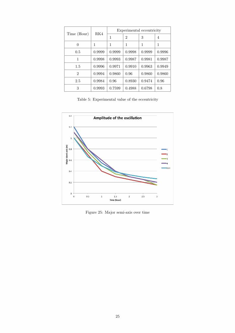
Time (Hour) RK4Experimental eccentricity

1 2 3 4

0 1 1 1 1 1

0.5 0.9999 0.9999 0.9998 0.9999 0.9996

1 0.9998 0.9993 0.9987 0.9981 0.9987

1.5 0.9996 0.9971 0.9910 0.9963 0.9949

2 0.9994 0.9860 0.96 0.9860 0.9860

2.5 0.9984 0.96 0.8930 0.9474 0.96

3 0.9993 0.7599 0.4988 0.6798 0.8

Table 5: Experimental value of the eccentricity

Figure 25: Major semi-axis over time

25

Figure 26

Figure 27

Figure 28

26

As for the period, the time was recorded for 100 swings, which equals to 9 mins 33.8 secs, and the

incertitude of chronometer 0.5s + and measurement error, assume 0.25s. Therefore the experimental period

of the Foucault pendulum equals to 5.738 ± 0.005s. While the theoretical period of the pendulum equals

to 5.701s. The relative error is 0.649%, small enough and we can call the experimental period is accurate.

This interval is due to the presence of air friction whose value is yet to be determined.

The experimental and analytical amplitude from fig. (25) correspond. Nonetheless there is a small

interval of difference, which is due to the air friction having the bigger value than predicted in numerical

analysis.

In fig. (26), after 4 experiments, the oscillation’s plane seems to rotate in clockwise direction only if it

is launched parallel to the beam. In fact, the oscillation’s plane did turn in the right direction in all our

experiments after 2 hours. The average observed angular velocity Ωob = (6.46417± 0.4)× 10−5 rad/s, by

comparing to the theoretical angular velocity at Grenoble ΩG = 5.15923 × 10−5 rad/s, the relative error

is 25.53% which is quite big.

In fig. (27), the experimental results have a bigger amplitude of minor demi-axis over time with respect

to the analytical results. Nevertheless, in the analytical results, the value of the perturbation constant

ε = 10−1 which is already quite big. We can assume that is due to the existence of transversal perturbation

with the bigger value than predicted coming from the pendulum’s surrounding. Therefore, to match the

experimental results, we have to either increase the value of ε, or completely assuming the new expression

of PE .

The same case is recorded in fig. (28), experimental E has the value much greater than predicted in

analytical results. It has the same reasoning as the fig. (27). However we noted that less vibration on the

thread during launching help reducing the development of ellipse during the oscillation.

The length of the experiment is limited by the frictional decrease of the amplitude and the increase of

the eccentricity. Nonetheless it is interesting to fire up a smoke machine in order to address the presence

of the Von Kármán vortex street of our experimental Foucault pendulum.

27

Figure 29: The launch of the pendulum’s oscillation

Figure 30: The view of the beam where the pendulum is suspended

28

4 Conclusion

4.1 Professional conclusion

The objective of our internship was to pursuit a complete study of the dynamics of the Foucault

pendulum, in case of idealised model as well as the real model, taking into account the existence of air

friction and eventually other external possible perturbations.

Our subject was mainly based on numerical study. The data obtained from the numerical study such as

the amplitude, the perturbation and the eccentricity give the theoretical results which are very important

as the base for the experiments that follows.

During our internship, only the final week was devoted to the experimental study and the validation of

the numerical and analytical data. This was due to the installation procedures of the Foucault pendulum

that took some time to finish. The existence of air friction was validated. Nonetheless, it was difficult to

verify its value, as well as the form and existence of additional perturbation occurred onto our pendulum

since we had only one week to do the experiments. Nonetheless, our experimental results served as a great

initiation for the researches that will take place henceforth.

4.2 Personal conclusion

This internship has been such a wonderful experience to both of us. Being able to participate in the

field of dynamical fluid mechanics has especially brought to us a great influence and knowledge to pursuit

our study in Masters. Not to forget the opportunity to work in the laboratory has also brought us the new

perspective on our career pursuit later on.

We have developed a great skill in studying with numerical data, mostly in dealing with how to simplify

the code in programming softwares, which leads to cutting the process and calculation time by half. That

is a very great deal in numerical study, and if we were to orient ourselves into the research, such time-saving

ability is very much welcome.

4.3 Professional & personal perspective

We have done what we could in the allocated time of our internship. The results are satisfying for what

time we had. All the objectives that we set at the beginning of the internship are achieved.

However since the pendulum was just freshly installed, the researchers will keep on experimenting with

the device to find and verify the analytical model. Moreover, according to our supervisor, the internship

will be extended next year to new students with more aspects of the pendulum to be discovered.

The possibility to pursuit the career in the research field is not possible to the students coming from

level L3. However the experience and the exposure gained from this internship here have greatly motivated

us that the research field is actually very interesting and very mind-opening. It has become a huge

encouragement for us to go to the "Master 2 Recherche".

29

References

[1] http://www.cleonis.nl/physics/phys256/foucault-pendulum.php

[2] http://www.mathworks.fr/fr/help/simulink/examples/modeling-a-foucault-pendulum.html

[3] http://www.school-for-champions.com/science/pendulum-equations.htm

[4] http://www.mpi-hd.mpg.de/astrophysik/HEA/internal/Numerical-Recipes/f16-1.pdf

30

A) APPENDIX 1: Numerical model in Scilab

\ begin spac ing 0 .1

############################################################

##########################################################

EQUILIBRIUM

############################################################

##########################################################

Y0(1)=1;

Y0(2)=0;

Y0(3)=0;

Y0(4)=0;

Y1= [ ] ;

f unc t i on [K]=pente (Y, f ,w2 , Omega2)

K(1)=Y( 2 ) ;

K(2)= f ∗Y(4)−w2∗Y(1)+Omega2∗Y( 1 ) ;

K(3)=Y( 4 ) ;

K(4)=− f ∗Y(2)−w2∗Y(3)+Approx1∗Y(3)−Rt∗Omega2∗ s i n ( phi )∗ cos ( phi )

endfunct ion

func t i on [ y]=RK44(Y0 , f ,w2 ,Omega2 , dt )

//M1

ytemp=Y0

P1=pente (ytemp , f ,w2 , Omega2)

//M2

ytemp=Y0+(dt∗P1 )/2 ;


//M3



//M4

ytemp=Y0+(dt∗P3 ) ;


[ y]=Y0+(dt /6)∗ (P1+2∗P2+2∗P3+P4)

i

endfunct ion

k=1;

Ya=ze ro s ( dt , 5 ) ;

Yb=ze ro s ( dt , 5 ) ;

Yc=ze ro s ( dt , 5 ) ;

f o r k=1:2

i f k==1 then ;

e l s e

Omega2=0;

Approx1=0;

end

Y0(1)=1;

Y0(2)=0;

Y0(3)=0;

Y0(4)=0;

Y1=[ ]

f o r i =1:( p r i n t s t ep )

t=( i −1)∗dT

f o r j =1: c a l c s t e p

[Y1]=RK44(Y0 , f ,w2 ,Omega2 , dt )

t=( i −1)∗dT+( j )∗ dt ;

Y0=Y1

end

// p r i n t f ("% f %f %f %f %f \n" , t ,Y1(1 ) ,Y1(2 ) ,Y1(3 ) ,Y1 ( 4 ) ) ;

i f k==1 then

Ya( i ,1)= t

Ya( i ,2)=Y1(1)

Ya( i ,3)=Y1(2)

Ya( i ,4)=Y1(3)

Ya( i ,5)=Y1(4)

e l s e

Yb( i ,1)= t

Yb( i ,2)=Y1(1)

Yb( i ,3)=Y1(2)

Yb( i ,4)=Y1(3)

Yb( i ,5)=Y1(4)

end

end

k=k+1

end

ii

f 1 = f i g u r e (1 )

c l f

p lot2d (Ya ( : , 1 ) ,Ya ( : , 2 ) , s t y l e = 4) // x en f onc t i on du temps

t i t l e ( ’ x en f onc t i on de temps avec Approximation ’ )

f 2 = f i g u r e (2 )

c l f

p lot2d (Yb( : , 1 ) ,Yb( : , 2 ) , s t y l e = 6) // x en f onc t i on du temps

t i t l e ( ’ x en f onc t i on de temps sans Approximation ’ )

f 4 = f i g u r e (4 )

c l f

p lot2d (Ya ( : , 1 ) , [ Ya ( : , 2 ) ,Yb ( : , 2 ) ] ) // x en f onc t i on du temps

t i t l e ( ’ comparison with and without approximation ’ , ’ f o n t s i z e ’ , 5 )

x l ab e l (" time t ( s ) " , ’ f o n t s i z e ’ , 4 )

y l ab e l (" p o s i t i o n x (m)" , ’ f o n t s i z e ’ , 4 )

r e c t =[7994 0 .5 7995 1 ] ; //a r e c t ang l e s p e c i f i e d in r a t i o o f the window s i z e

zoom_rect ( r e c t )

############################################################

##########################################################

ERROR RK4 RK2

############################################################

##########################################################

c l e a r

format long ; %view more p r e c i s i o n o f the r e s u l t s

g l oba l phi g l thetadot dt1 dt2 dt3 dt4 t f i n a l p r i n t s t ep dT f w w2 Y0 Y Y1 Ye x_analytique Fd1 Fd2

%ex t e rna l parameters

phi =0.788675503881750426; %l a t i t u d e o f Grenoble

g=9.8250; %g r a v i t a t i o n a l a c c e l e r a t i o n

l =8; %pendulum ’ s l ength

thetadot =0.00007292115855; %earth ’ s angular r o t a t i o n a l speed

r =0.11; %rad iu s o f the bob

A=pi ∗ r ∗ r ; %A i s the cros s−s e c t i o n a l area (m2)

f r i c t i on_cond =1; %%f r i c t i o n cond i t i on

%f r i c t i o n non−e x i s t an t=1

iii

%l i n e a r f r i c t i o n=2

%quadrat i c f r i c t i o n=3

%t o t a l f r i c t i o n=4

%i n t e r n a l parameters

dt1 =0.1 ; %s t ep s f o r Runge−Kutta c a l c u l a t i o n

dt2 =0.05;

dt3 =0.025;

dt4 =0.0125;

t f i n a l =1000;

p r i n t s t ep=t f i n a l ∗10 ;

dT=t f i n a l / p r i n t s t ep ;

%constant va lue s

f=2∗ thetadot ∗ s i n ( phi ) ;

w=sq r t ( g/ l ) ;

w2=w∗w;

%i n i t i a l c ond i t i on s

Y0= [ ] ;

Y0(1)=1;

Y0(2)=0;

Y0(3)=0;

Y0(4)=0;

%matrix c r e a t i on

Y=ze ro s ( p r i n t s t ep +1 ,33) ;

Y1= [ ] ;

Ye=ze ro s ( 4 , 5 ) ;

Fd1=6∗pi ∗0.000019∗ r ; %c o e f f i c i e n t l i n e a r f r i c t i o n

Fd2=0.5∗1 .275∗0 .47∗ pi ∗A; %c o e f f i c i e n t f r i c t i o n quadrat ique

i f f r i c t i on_cond==1

Fd1=0;

Fd2=0;

e l s e i f f r i c t i on_cond==2

Fd2=0;

e l s e i f f r i c t i on_cond==3

Fd1=0;

end

%i n i t i a l c ond i t i on s put in to f i n a l −value matrix

iv

Y(1 ,1)=0; %t

f o r p=0:3

Y(1 ,4∗p+2)=Y0 ( 1 ) ; %x

Y(1 ,4∗p+3)=Y0 ( 2 ) ; %dx/dt

Y(1 ,4∗p+4)=Y0 ( 3 ) ; %y

Y(1 ,4∗p+5)=Y0 ( 4 ) ; %dy/dt

end

%value o f s tep put in to l og ( dt)− l og ( e r r o r ) t ab l e

Ye(1 ,1)= dt1 ;

Ye(2 ,1)= dt2 ;

Ye(3 ,1)= dt3 ;

Ye(4 ,1)= dt4 ;

%matrix c r e a t i on f o r f i n a l va lue matrix ’ s c a l c u l a t i o n

Y0

FE_RK4_step1 ;

FE_RK4_step2 ;

FE_RK4_step3 ;

FE_RK4_step4 ;

FE_RK2_step1 ;

FE_RK2_step2 ;

FE_RK2_step3 ;

FE_RK2_step4 ;

s o l u t i onana l y t i qu e1 ;

%f i l l the l og ( dt)− l og ( e r r o r ) t ab l e

f o r d=1:4

Ye(d ,3)= sq r t ( (Ye(d,2)− x_analytique )^2 ) ;

Ye(d ,5)= sq r t ( (Ye(d,4)− x_analytique )^2 ) ;

end

Ye %show the e r r o r t ab l e

v

%pr in t the r e s u l t

%f1 = f i g u r e ( 1 ) ;

%c l f ;

%subplot ( 1 2 1 ) ;

%p lo t (Y( : , 1 ) , [Y( : , 2 ) Y( : , 6 ) ] ) ; %x et y en f onc t i on du temps

%x l ab e l ( ’ x et y en f onc t i on de temps ’ ) ;

%subplot ( 1 2 2 ) ;

%p lo t (Y( : , 2 ) ,Y( : , 4 ) ) ; %y en f onc t i on du x

%x l ab e l ( ’ y en f onc t i on de x ’ ) ;

f 1 = f i g u r e ( 1 ) ;

c l f ;

p l o t ( l og (Ye ( : , 1 ) ) , [ l og (Ye ( : , 3 ) ) l og (Ye ( : , 5 ) ) ] , ’ o− ’)

l egend ( ’RK4’ , ’RK2’ )

x l ab e l ( ’ l og ( dt ) ’ )

y l ab e l ( ’ l og ( e r r o r ) ’ )

t i t l e ( ’ Error f o r Pendulums Pos i t i on at t f i n a l =1000 ’)

f 2 = f i g u r e ( 2 ) ;

c l f ;

p l o t (Y( : , 1 ) , [Y( : , 2 ) Y( : , 4 ) ] )

l egend ( ’ po s i t i on−x ’ , ’ po s i t i on−y ’ )

x l ab e l ( ’Time ( second ) ’ )

y l ab e l ( ’ Po s i t i on ( meter ) ’ )

t i t l e ( ’ O s c i l l a t i o n o f the pendulum ’ )

f 3 = f i g u r e ( 3 ) ;

c l f ;

p l o t (Y( : , 2 ) ,Y( : , 4 ) )

x l ab e l ( ’ po s i t i on−x ( meter ) ’ )

y l ab e l ( ’ po s i t i on−y ( meter ) ’ )

t i t l e ( ’ Pendulum" s movement a f t e r 1 day ’ )

#################

globa l dt1 p r i n t s t ep dT f w2 Y Y0 Ye Fd1 Fd2

Z0 = [ ] ;

Z0(1)=Y0 ( 1 ) ;

Z0(2)=Y0 ( 2 ) ;

Z0(3)=Y0 ( 3 ) ;

Z0(4)=Y0 ( 4 ) ;

dt=dt1 ;

vi

c a l c s t e p=dT/dt ;

%c a l c u l a t e f i n a l va lue f o r t=i : " t f i n a l " with v i s u a l i s a t i o n o f va lue every " p r i n t s t ep "


t=( i −1)∗dT;


[Y1]=RK22(Z0 , f , w2 , dt , Fd1 , Fd2 ) ;

t=( i −1)∗dT+( j )∗ dt ;

Z0=Y1 ;

end

%p r i n t f ("% f %f %f %f %f \n" , t ,Y1(1 ) ,Y1(2 ) ,Y1(3 ) ,Y1 ( 4 ) ) ;

Y( i +1,1)= t ;

Y( i +1,18)=Y1 ( 1 ) ;

Y( i +1,19)=Y1 ( 2 ) ;

Y( i +1,20)=Y1 ( 3 ) ;

Y( i +1,21)=Y1 ( 4 ) ;

end

Ye(1 ,4)=Y1 ( 1 ) ;

#####################

globa l dt1 p r i n t s t ep dT f w2 Y Y0 Ye Fd1 Fd2

Z0 = [ ] ;

Z0(1)=Y0 ( 1 ) ;

Z0(2)=Y0 ( 2 ) ;

Z0(3)=Y0 ( 3 ) ;

Z0(4)=Y0 ( 4 ) ;

dt=dt1 ;


%c a l c u l a t e f i n a l va lue f o r t=i : " t f i n a l " with v i s u a l i s a t i o n o f va lue every " p r i n t s t ep "


vii

t=( i −1)∗dT;


[Y1]=RK44(Z0 , f , w2 , dt , Fd1 , Fd2 ) ;

t=( i −1)∗dT+( j )∗ dt ;

Z0=Y1 ;

end

%p r i n t f ("% f %f %f %f %f \n" , t ,Y1(1 ) ,Y1(2 ) ,Y1(3 ) ,Y1 ( 4 ) ) ;

Y( i +1,1)= t ;

Y( i +1,2)=Y1 ( 1 ) ;

Y( i +1,3)=Y1 ( 2 ) ;

Y( i +1,4)=Y1 ( 3 ) ;

Y( i +1,5)=Y1 ( 4 ) ;

end

Ye(1 ,2)=Y1 ( 1 ) ;

############################################################

##########################################################

ERROR RK44 ANALYTIC

############################################################

##########################################################

k=1;

Ya=ze ro s ( dt , 6 ) ;

Yb=ze ro s ( dt , 6 ) ;

Yc=ze ro s ( dt , 1 ) ;

Y1=[ ]

Fd1=0;

Fd2=0;


t=( i −1)∗dT


[Y1]=RK44(Y0 , dt )

t=( i −1)∗dT+( j )∗ dt ;

Y0=Y1

viii

end

// p r i n t f ("% f %f %f \n" , t ,Y1(1 ) , r e a l ( z ( i +1)) ) ;

Yb( i ,1)= t

Yb( i ,2)=Y1(1)

Yb( i ,3)=Y1(2)

Yb( i ,4)=Y1(3)

Yb( i ,5)=Y1(4)

Yb( i ,6)= sq r t (Y1(2)∗Y1(2)+Y1(4)∗Y1(4 ) )

Yc( i ,1)= sq r t ( ( r e a l ( z ( i +1))−Yb( i , 2 ) ) ∗ ( r e a l ( z ( i +1))−Yb( i ,2 ) )+( imag ( z ( i +1))−Yb( i , 4 ) ) ∗ ( imag ( z ( i +1))−Yb( i , 4 ) ) )

//Yc( i ,2)= sq r t ( ( r e a l ( z ( i +1))−Yb( i , 2 ) ) ∗ ( r e a l ( z ( i +1))−Yb( i ,2 ) )+( imag ( z ( i +1))−Yb( i , 4 ) ) ∗ ( imag ( z ( i +1))−Yb( i , 4 ) ) ) /max( ’ ( s q r t ( r e a l ( z ( i +1))∗ r e a l ( z ( i +1))+imag ( z ( i +1))∗ imag ( z ( i +1) ) ) ) ’ )

Yc( i ,3)= sq r t ( r e a l ( z ( i +1))∗ r e a l ( z ( i +1))+imag ( z ( i +1))∗ imag ( z ( i +1)))

end

t=0: t f i n a l / p r i n t s t ep : t f i n a l ;

f 1 = f i g u r e (1 )

c l f

p lot2d (Yb(1 : 5 0 0 , 1 ) ,Yb(1 : 5 00 , 2 ) , s t y l e = 20) // x en f onc t i on du temps

plot2d ( t ( 1 : 5 0 0 ) , r e a l ( z ( 1 : 0 ) ) , s t y l e = 32) // x en f onc t i on du temps

// plot2d ( t (99/100∗ p r i n t s t ep : p r i n t s t ep ) ,Yb(99/100∗ p r i n t s t ep : p r in t s t ep , 2 ) , s t y l e = 32) // x en f onc t i on du temps

// plot2d ( t (99/100∗ p r i n t s t ep : p r i n t s t ep ) , r e a l ( z (99/100∗ p r i n t s t ep : p r i n t s t ep ) ) , s t y l e = 19) // x en f onc t i on du temps

t i t l e ( ’ x p o s i t i o n as a func t i on o f time ’ , ’ f o n t s i z e ’ , 6 )

x l ab e l (" time ( s ) " , ’ f o n t s i z e ’ , 4 )

y l ab e l (" e r r o r (m)" , ’ f o n t s i z e ’ , 4 )

l egends ( [ ’ a n a l y t i c a l s o lu t i on ’ ; ’ Runge−Kutta−44 so lu t i on ’ ] , [ 1 9 , 3 2 ] , opt=" l r " , f ont_s i z e=3 )

l i n e s (0 ) // d i s a b l e s v e r t i c a l paging

a=get (" current_axes ")// get the handle o f the newly c rea ted axes

a . axe s_v i s i b l e="on " ; // makes the axes v i s i b l e

a . f on t_s i z e =6; // s e t the t i c s l a b e l f ont s i z e

a . x_locat ion="bottom " ; // s e t the x ax i s p o s i t i o n

f2 = f i g u r e (2 )

c l f

p lot2d (Yb(1 : 5 0 0 , 1 ) ,Yc ( 1 : 5 00 , 1 ) , s t y l e = 19) // x en f onc t i on du temps

t i t l e ( ’ ab so lu t e e r r o r between RK44 et ana ly t i c ’ , ’ f o n t s i z e ’ , 5 )






ix

a . f ont_s i z e =5; // s e t the t i c s l a b e l f ont s i z e


//a . data_bounds = [1 , 0 , 1 ; 0 , 1 50000 , 1 ] ; // s e t the boundary va lue s f o r the x , y and z coo rd ina t e s .

//a . sub_tics = [ 5 , 0 ] ;

//a . l abe l s_font_co lo r =1;

//a . box="o f f " ;


f 3 = f i g u r e (3 )

c l f

p lot2d (Yb(997/1000∗ p r i n t s t ep : p r in t s t ep , 1 ) ,Yb(997/1000∗ p r i n t s t ep : p r in t s t ep , 2 ) , s t y l e = 32) // x en f onc t i on du temps

plot2d ( t (997/1000∗ p r i n t s t ep : p r i n t s t ep ) , r e a l ( z (997/1000∗ p r i n t s t ep : p r i n t s t ep ) ) , s t y l e = 19) // x en f onc t i on du temps

// plot2d ( t (99/100∗ p r i n t s t ep : p r i n t s t ep ) ,Yb(99/100∗ p r i n t s t ep : p r in t s t ep , 2 ) , s t y l e = 32) // x en f onc t i on du temps

// , r e c t = [997 . 8 , 0 . 98 , 998 , 1 ] p lot2d ( t (99/100∗ p r i n t s t ep : p r i n t s t ep ) , r e a l ( z (99/100∗ p r i n t s t ep : p r i n t s t ep ) ) , s t y l e = 19) // x en f onc t i on du temps

t i t l e ( ’ x p o s i t i o n as a func t i on o f time ’ , ’ f o n t s i z e ’ , 6 )



l egends ( [ ’ a n a l y t i c a l s o lu t i on ’ ; ’ Runge−Kutta−44 so lu t i on ’ ] , [ 1 9 , 3 2 ] , opt="?" , f ont_s i z e=3 )






############################################################

##########################################################

TRANSVERSAL PERTURBATION

############################################################

##########################################################

c l e a r

format ( ’ v ’ , 1 0 ) ;

chd i r ( ’ /home/thom/Bureau/Stage /Prog/Sclb ’ ) ;

phi =0.788675503;

g=9.8250;

l =8;

Omega=0.0000729211;

Rt=6379140;

dt=0.01

f=2∗Omega∗ s i n ( phi ) ;

n=2∗%pi /(Omega∗dt ) ;

w=sq r t ( l /g ) ;

w2=w∗w

x

wp=1/ sq r t (2 )

T=2∗%pi /w;

r =0.11; // rad iu s o f the bob (m)

A=%pi ∗ r ∗ r ; //A i s the cros s−s e c t i o n a l area (m2)

Y=ze ro s ( dt , 5 ) ;

t f i n a l =300000

p r i n t s t ep =12000000;

dT=t f i n a l / p r i n t s t ep ;


Omega2=Omega∗Omega ;

Approx1=f ∗ f /4 ;

eps =0.0001;


// c o e f f i c i e n t f r i c t i o n l i n a i r e

Fd1=6∗%pi ∗0.00019∗ r /45

// c o e f f i c i e n t f r i c t i o n quadrat ique

Fd2=0.5∗1.275∗0.47∗% pi ∗A/45 ;

Y0(1)=1;

Y0(2)=0;

Y0(3)=0;

Y0(4)=0;

Y1= [ ] ;

f unc t i on [K]=pente (Y)

x=Y(1)

xdot=Y(2)

y=Y(3)

ydot=Y(4)

K(1)=xdot ;

K(2)= f ∗ydot−w2∗x−Fd2∗abs ( xdot )∗ xdot ;

K(3)=ydot ;

K(4)=− f ∗xdot−w2∗y−Fd2∗abs ( ydot )∗ ydot ;

endfunct ion

func t i on [ y]=RK44(Y0 , dt )

//M1

ytemp=Y0

P1=pente ( ytemp)

xi

//M2


P2=pente ( ytemp)

//M3


P3=pente ( ytemp)

//M4

ytemp=Y0+(dt∗P3 ) ;

P4=pente ( ytemp)

[ y]=Y0+(dt /6 )∗ ( (P1+2∗P2+2∗P3+P4) )

endfunct ion

j =1;

k=1;

Fd2=0;

f i d 1=mopen ( ’ trans−r e s u l t a t−Fd2 0 ’ , ’w+ ’) ;

Y0(1)=1;

Y0(2)=0;

Y0(3)=0;

Y0(4)=0;

Y1=[ ]


t=( i −1)∗dT


[Y1]=RK44(Y0 , dt )

t=( i −1)∗dT+( j )∗ dt ;

Y0=Y1

end

mfpr in t f ( f id1 , ’% f %f %f %f \n ’ , t ,Y1(1 ) ,Y1(3 ) , s q r t (Y1(1)∗Y1(1)+Y1(3)∗Y1( 3 ) ) )

end

mclose ( f i d 1 ) ;

############################################################

##########################################################

DATA READING

c l e a r

chd i r ( ’ /home/thom/Bureau/Stage /Prog/Sclb ’ ) ;

xii

p r i n t s t ep =600000

nbpoints=30000

j=1

f i d 2=mopen ( ’ f i n a a l −i d ea l ’ ) ;

f o r i =1: nbpoints

A=mfscanf ( p r i n t s t ep /nbpoints , f id2 ,"% lg %lg %lg %lg %lg %lg " ) ;

Z1 ( i ,1)=A(1 ,1 )

Z1( i ,2)=A(1 ,2 )

Z1( i ,3)=A(1 ,3 )

Z1( i ,4)=A(1 ,4 )

Z1( i ,5)=A(1 ,5 )

Z1( i ,6)=A(1 ,6 )

end

f i d 3=mopen ( ’ f i n a a l −Fd1 ’ ) ;


B=mfscanf ( p r i n t s t ep /nbpoints , f id3 ,"% lg %lg %lg %lg %lg %lg " ) ;

Z2 ( i ,1)=B(1 , 1 )

Z2( i ,2)=B(1 , 2 )

Z2( i ,3)=B(1 , 3 )

Z2( i ,4)=B(1 , 4 )

Z2( i ,5)=B(1 , 5 )

Z2( i ,6)=B(1 , 6 )

end

f i d 4=mopen ( ’ f i n a a l −Fd2 ’ ) ;


C=mfscanf ( p r i n t s t ep /nbpoints , f id4 ,"% lg %lg %lg %lg %lg %lg " ) ;

Z3 ( i ,1)=C(1 , 1 )

Z3( i ,2)=C(1 , 2 )

Z3( i ,3)=C(1 , 3 )

Z3( i ,4)=C(1 , 4 )

Z3( i ,5)=C(1 , 5 )

Z3( i ,6)=C(1 , 6 )

end

E=ze ro s ( nbpoints , 2 ) ;

xiii

i=1


E( i ,1)=Z1( i , 1 ) ;

E( i ,2)= sq r t (Z1 ( i , 3 )∗Z1( i ,3)+Z1( i , 2 )∗Z1( i , 2 ) ) ;

end


E( i ,1)=Z2( i , 1 ) ;

E( i ,2)= sq r t (Z2 ( i , 3 )∗Z2( i ,3)+Z2( i , 2 )∗Z2( i , 2 ) ) ;

end


E( i ,1)=Z3( i , 1 ) ;

E( i ,2)= sq r t (Z3 ( i , 3 )∗Z3( i ,3)+Z3( i , 2 )∗Z3( i , 2 ) ) ;

end

f2 = f i g u r e (2 )

c l f

p lot2d (Z1 ( : , 1 ) , Z1 ( : , 2 ) , s t y l e= 16) // d i r e c t i v i t en f onc t i on du temp

plot2d (Z2 ( : , 1 ) , Z2 ( : , 2 ) , s t y l e= 14) // d i r e c t i v i t en f onc t i on du temp

plot2d (Z3 ( : , 1 ) , Z3 ( : , 2 ) , s t y l e= 32) // d i r e c t i v i t en f onc t i on du temp

t i t l e ( ’ plan view o f the bob through time ’ , ’ f o n t s i z e ’ , 6 )

x l ab e l ("x (m)" , ’ f o n t s i z e ’ , 6 )

y l ab e l ("y (m)" , ’ f o n t s i z e ’ , 6 )

l egends ( [ ’ i d ea l ’ ; ’ l i n e a r f r i c t i o n ’ ; ’ quadrat i c f r i c t i o n ’ ] , [ 1 6 , 1 4 , 3 2 ] , opt=" l r " , f on t_s i z e=5 )






a . data_bounds = [1 , 0 , 1 ; 0 , 1 50000 , 1 ] ; // s e t the boundary va lue s f o r the x , y and z coo rd ina t e s .

a . sub_tics = [ 5 , 0 ] ;

a . l abe l s_font_co lo r =1;

a . box="o f f " ;

mclose

############################################################

##########################################################

\end spac ing

xiv

A Numerical and Experimental Study of the Dynamics of the … · · 2018-03-27of the Dynamics of...

Documents

Transcript of A Numerical and Experimental Study of the Dynamics of the … · · 2018-03-27of the Dynamics of...