A novel test configuration design method for inverse ...

of 42

A novel test configuration design method for inverse identification of in-plane moduli of a composite plate under the PFEUM framework M.Z. Siddiquia, S.Z. Khana,b *, , M.A. Khanc, M. Shahzadd, , K.A. Khane, S. Nisara

aDepartment of Engineering Sciences, PN Engineering College, National University of Sciences and Technology (NUST), Karachi, Pakistan bDepartment of Mechanical Engineering, Faculty of Engineering, Islamic University of Madinah, Madinah, PO Box 170, Kingdom of Saudi Arabia cSchool of Aerospace, Transport and Manufacturing, Cranfield University, Cranfield, UK dSpace and Upper Atmosphere Research Commission (SUPARCO), Karachi, Pakistan eDepartment of Aerospace Engineering, Khalifa University of Science, Technology and Research (KUSTAR), Abu Dhabi, UAE

*Corresponding Author

Abstract We propose a novel sensitivity based approach which predicts and explains the accuracy of

material parameter identification for a composite plate using the Projected Finite Element

Update Method (PFEUM). A typical experiment using the PFEUM technique involves a plate

specimen held at three or four supports and bent under the application of a point load. Two-

Dimensional Digital Image Correlation (2D-DIC) is used to measure the pseudo displacements

resulting from the projection of out-of-plane deflection of the plate onto the image plane. A cost

function relating the projected numerical and experimental displacement fields is then

minimized to obtain the material parameters. It is shown that the contribution of a specific

material parameter in the observed displacement field influences the accuracy of its

identification. The contributions from material parameters are first quantified in terms of

sensitivity criterion which may be tailored by changing the elements of test configuration like

location of supports, the load application point and the specimen geometry. Several test

configurations are designed by maximizing the sensitivities corresponding to individual material

parameters. The relevance of proposed sensitivity criterion in these configurations is then

e805814

Text Box

Strain, Volume 54, Issue 5, 2018, Article number e12280 DOI: 10.1111/str.12280

e805814

Text Box

Published by Wiley. This is the Author Accepted Manuscript issued with: Creative Commons Attribution Non-Commercial License (CC:BY:NC 4.0). The final published version (version of record) is available online at DOI:10.1111/str.12280. Please refer to any applicable publisher terms of use.

of 42

validated through material identification in simulated experiments with added Gaussian noise.

Finally, a thin CFRP plate is tested under these configurations to demonstrate the practical use

of this approach. The proposed approach helps in robust estimation of the in-plane elastic moduli

from a bent composite plate with a simple 2D-DIC setup without requiring measurement of the

actual plate deflection or curvatures.

Keywords: 2D field measurements; Inverse identification; Finite Element Model Update method;

Out-of-plane motion; Perspective projection; Parameter sensitivity; In-plane Elastic Moduli

1.1 Corresponding author contact:

Sohaib Zia Khan

Email: [email protected]

Phone: +92 333 2273 100

Address: PG Building, PNEC, Habib Rehmatullah Road, National University of Sciences and

Technology, Karachi, Pakistan 75350.

mailto:[email protected]

of 42

1 Introduction The cost benefit offered by laminated composites has brought about their widespread use in

different industrial and household applications and has resulted in light weight products being

produced at increasingly competitive costs. The weight reduction, however, also requires that

the precise material response be known beforehand at the time of product design to avoid in-

service failures. Characterization of the mechanical response of laminated composites presents

unique challenges due to their anisotropic nature. In general, the displacement response of

composites involves contributions from more than one material parameters [1]. The ASTM

standards for characterization of laminated composites provide specific guidelines for specimen

preparation and testing. Individual test guidelines, detailing the geometry and loading conditions,

ensure that the displacement response from different material parameters are decoupled and a

homogeneous displacement field is achieved which is mandatory when direct measurement of

individual material parameters is sought [2]. These direct methods, however, are limited in their

application as they require a large number of specimens and expendable strain gauges for

complete characterization of material response [3].

The limitations present in the direct methods may be overcome if the test method is able to

utilize heterogeneous displacement fields resulting in relaxation of the stringent geometry and

loading requirements [4]. Recent research in this area has resulted in development of a range of

inverse methods which precisely require the displacement response to be heterogeneous thus

enabling identification of multiple material parameters from a single test. Contrary to the

classical identification techniques where heterogeneous displacement or strain fields are a

limiting condition, a variety of inverse methods are now available that make use of this

heterogeneous information [5]. This paper deals with a particular application of an inverse

method called the Finite Element Model Updating technique – also referred to as the Finite

Element Update Method (FEUM) [6, 7].

The FEUM technique is applied using displacement [8] as well as natural frequencies [9, 10] for

identification of material constitutive parameters. In a typical FEUM problem, a set of unknown

constitutive parameters is assumed and using a FE model, a numerical displacement (or strain)

field is generated. A similar displacement field is found by experimental measurement on the

of 42

specimen whose material properties are to be determined. A cost function comprising of the

displacement gap between the experimental and Finite Element (FE) solution of the surface

response is then minimized in an iterative fashion to yield the material parameters being sought.

[11]. Although full-field data on the whole surface of the specimen is desirable, the technique is

equally applicable when the full-field data is available in only part of the domain [12].

Several researchers have adopted the FEUM based techniques for identification of material

constitutive parameters in composite materials. For example Lecompte et al. [1] used cruciform

shaped specimens made from glass fiber reinforced epoxy in biaxial tension. Bruno et al. [13]

conducted study on the identification of elastic properties of unidirectional Graphite/PEEK using

a plate specimen under flexural loading. In-plane properties of an orthotropic laminate were

determined by Molimard et al. [14] using a thin plate specimen with a central hole loaded in

tension. Wang and Kam [15] identified the elastic parameters of an orthotropic plate made from

graphite/epoxy laminate. The rectangular plates were tested in a CCCC boundary condition (CCCC

denotes clamping at all four edges, each C representing an edge) and loaded with two types of

loads: a point load at the center and a distributed pressure. A T-shaped specimen subjected to

complex stress state was employed by Grédiac et al. [16] for identification of in-plane constitutive

parameters. In addition to lab scale specimens, the inverse methods are also applicable to real

structures. For example, in vivo characterization of anisotropic properties of human skin on a

volar forearm was performed by Meijor et al. [17]. The FEUM approach was also used for

identification of interlaminar fracture behavior of a unidirectional thermoset composite material

by Mathieu et al. [18].

The tailoring of test configuration parameters has been studied earlier for design of an optimal

test configuration for inverse identification of constitutive parameters in laminated composites.

However, most of the earlier work in this direction relates to inverse identification using the

Virtual Fields Method (VFM) [19] which relies on satisfaction of the global or weak form of

equilibrium equations. The Finite Element Update Method (FEUM) has attracted little attention

in this regard due to the absence of analytical relations to evaluate the sensitivity of identified

parameters. The process of selection of optimized virtual fields for inverse identification yields

noise sensitivity coefficients corresponding to the orthotropic stiffness’s [20]. Pierron et al [21]

of 42

have presented an optimization strategy which uses these sensitivity coefficients for constructing

a cost function balancing the sensitivities of all material parameters in a composite specimen.

The standard Unnotched Iosipescu (UI) test was used for the study with displacement

measurements done by speckled interferometry. A similar cost function based on the global

noise sensitivity coefficients normalized with respect to the maximum plate deflection have been

used in [3, 22]. The authors used grid method for measurement of curvatures in a bent composite

plate specimen while the identification was done using the VFM. A numerical simulator for design

of an optimal test configuration is presented by Rossi and Pierron [23] which is able to accurately

model the parameters associated with the UI test. Under the VFM framework, the authors did a

comprehensive study highlighting the effects of stress limit scaling, displacement field anisotropy,

smoothing of strain field and the influence of missing data near the specimen boundary on

parameter identification. In another research [24], the authors used this numerical simulator to

study the effect of DIC settings in terms of identification error for selection of optimal test

settings.

The displacement response of the specimen surface can also be captured by the optical

techniques like Two- or Three-dimensional Digital Image Correlation (DIC) [25]. Thetwo-

dimensional Digital Image Correlation (2D-DIC) measures the in-plane surface displacements by

comparing two images taken before and after the surface deformation [26, 27]. This method has

benefits like ease of setup, less requirement of computation power as well as ease of calibration

and low cost. In this method, a single camera is placed for taking images of the deforming surface

in a way that the optical axis of the camera is parallel to the outward normal of the surface under

consideration [28]. The specimens are tested with the 2D-DIC. They are generally either flat and

subjected to in-plane loading (tension, compression, shear, biaxial or a combination of these

loading conditions) [29, 30]; or at least the surface under observation has predominantly in-plane

deformation [31]. Because of the simplicity and other benefits that it offers, 2D-DIC is employed

in a large number of applications [32]. The out-of-plane displacements cannot be detected and

result in pseudo displacements seen as artificial strains in the DIC output [33, 34].

In plate bending experiments,the displacements are chiefly out-of-plane while the contribution

of in-plane displacements is minimal. For such an arrangement, application of 2D-DIC results in

of 42

measurement of a projected displacement field [29] which can only be utilized for identification

of material constitutive parameters using a displacement gap based FEUM technique [30]. The

Projected Finite Element Update Method (PFEUM) [35] relies on the minimization of a

displacement gap between measured and computed displacement fields projected onto the

image plane of camera. The primary advantage of this approach is that it allows use of a simple

2D-DIC setup for material identification using specimens undergoing three-dimensional

deformation; thus, becomes cost effective and computationally reasonable. The details of the

mathematical development of the PFEUM technique can be found in [29, 30].

In this research, we propose a novel sensitivity based method for design of a test configuration

for material parameter identification using the PFEUM technique. The proposed method

produces displacement fields with controlled contributions from the material parameters. The

test setup is designed such that it allows alteration in the heterogeneity of the observed

displacement field by controlling the setup parameters like position of supports, load location,

fiber orientation and the aspect ratio. In the next section, a matrix based description of the

equations of perspective projection developed earlier in [35] is given using the homogeneous

coordinates. The inverse problem under the PFEUM framework is then reformulated. Later,

sensitivity criterion for contribution of different material parameters in overall displacement field

is derived using the FE simulations. At the end experimental data, for identification of in-plane

elastic moduli of a CFRP plate, is presented to verify the validity of sensitivity criterion based on

some tailored test configurations.

2 Method

2.1 Projected Finite Element Update Method

In this article, a compact matrix based description of the PFEUM technique is given which helps

in the development of sensitivity criterion for design of test configuration and is conveniently

applicable in a computer program. We start by considering the general case of projecting a point

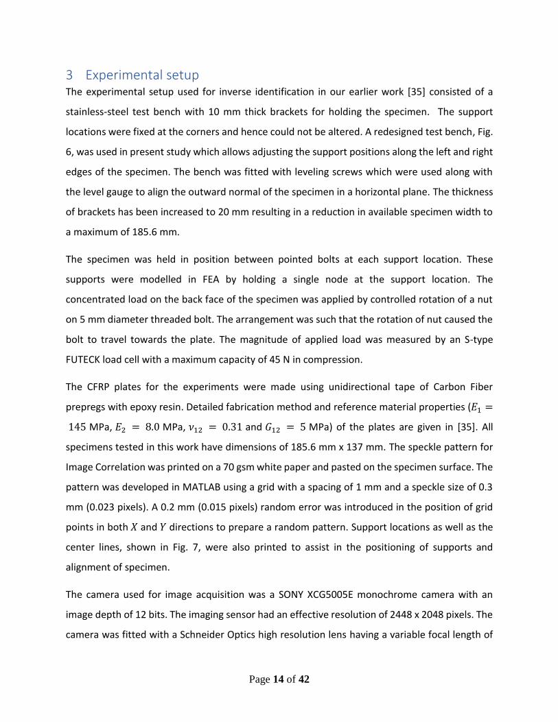
in space 𝑝(𝑥, 𝑦, 𝑧) onto the image plane of an imaging system as shown in Fig. 1(a). A right

handed Cartesian coordinate system is chosen to be parallel to the conventional image

coordinate system with y-axis pointing downwards. Let 𝑣(0,0, −𝑧0) be a point away from the

image plane which lies on the optical axis. The perspective projection of point 𝑝 on the image

of 42

plane is the intersection of line 𝑣𝑝̅̅̅̅ with the image plane and is identified as 𝑝′′(𝑥′′, 𝑦′′, 𝑧′′). The

point 𝑣 here is the center of perceptivity or viewpoint. The image plane normal, 𝑛, and the view

direction are coincident with the z-direction.

A 2D version of Fig. 1(a) is shown in Fig. 1(b). Using similarity of triangles, we can directly write

as

𝑦

𝑦′′=

𝑧0−𝑧

𝑧0=

𝑥

𝑥′′ (1)

From where the position of projected point may be computed as

𝑥′′ =𝑧0

𝑧0−𝑧𝑥 , 𝑦′′ =

𝑧0

𝑧0−𝑧 𝑦

Since z may be negative or positive, we can generalize these equations as

𝑥′′ =𝑧0

𝑧0+𝑧𝑥 , 𝑦′′ =

𝑧0

𝑧0+𝑧 𝑦 (2)

Equations (2) is similar to those derived earlier in [30] with ∆𝑍 replaced by 𝑧. The equations were

earlier derived for a deforming body with ∆𝑍 being the out-of-plane displacement of a point

initially lying on the image plane. However, the description presented here is more generic and

is derived directly from the principles of projective geometry [36]. The current description allows

projection of any point in space irrespective of its underlying deformation or loading history.

It is interesting to note that the camera model given by equations (2), which forms the basis of

pinhole camera model [25], is nonlinear in 𝑧 and hence cannot be represented by simple matrix

multiplication. To make the camera model linear, we can use the homogeneous coordinates [25]

which represent points and lines in the projective space using vectors with four coordinates –

also called 4 vectors. Conversion from projective to Euclidian space is achieved by dividing the

first three coordinates with the fourth coordinate which serves as a scaling parameter. From the

geometry of perspective projection any point on the line joining points 𝑝 and 𝑣, and intersecting

the image plane has coordinates of the form

𝑝′ = 𝑀𝑝 (3)

and,

of 42

𝑀 = 𝑛𝑇𝑣 + (𝑛. 𝑣)𝐼4 (4)

Where, 𝐼4 is the 4 × 4 identity matrix. Equation (3) gives the linear form of the pinhole camera

model and permits the perspective projection of a point to be taken by simple matrix

multiplication. The perspective projection matrix 𝑀 is a linear transformation which maps points

in the three-dimensional space to their corresponding projection points on the image plane. For

the proof of equation (4) refer to [37].

Let 𝑝(𝑥, 𝑦, 𝑧, 1) and 𝑣(0,0, −𝑧0, 1) be the homogeneous coordinates of the points 𝑝 and 𝑣

respectively, and let the image plane normal towards the viewpoint be represented by

𝑛(0,0, −1,0) as shown in Fig. 1(a). Substituting the values in equation (4) gives

𝑀 = [

−𝑧0 0 0 00 −𝑧0 0 00 0 0 00 0 −1 −𝑧0

]

And since 𝜆𝑀𝑝 = λ𝑝′, we can divide M by a scalar (−𝑧0) to give

𝑀 =

[ 1 0 0 00 1 0 00 0 0 0

0 01

𝑧01]

(5)

Substituting back in equation (3) gives

{

𝑥′𝑦′

𝑧′𝑤

} =

[ 1 0 0 00 1 0 00 0 0 0

0 01

𝑧01]

{

𝑥𝑦𝑧1

}

Solving for (𝑥′, 𝑦′, 𝑧′) and 𝑤 gives the homogeneous coordinates of the projection on image

plane as

𝑥′ = 𝑥 , 𝑦′ = 𝑦 , 𝑧′ = 0 , 𝑤 =𝑧+𝑧0

𝑧0

Where, 𝑤 is a scaling parameter used to convert homogeneous coordinates to Euclidian

coordinates as

of 42

𝑥′′ =𝑥′

𝑤, 𝑦′′ =

𝑦′

𝑤 (6)

Substituting for 𝑤 in equation (6) yields the Euclidian coordinates identical to those in equation

(2). Hence the linear form presented in equation (3) gives the same results as equation (2) but is

preferred because of the ease of application. The perspective projection matrix needs to be

evaluated only once and thereafter only a simple matrix multiplication can be used to project a

set of points from the three-dimensional space to the image plane. The hierarchy of projective

transformations also allow multiple transformations to be concatenated in a single expression

[38]. It is therefore possible to combine the rigid body motion of a body with subsequent

projection in a single step as

𝑝′ = 𝑀𝐶𝑝 (7)

Where, 𝐶 = [𝑅 𝑡] is a 4 × 4 matrix that applies rigid body transformation to 𝑝 with 𝑅 and 𝑡

representing the rigid body rotation and translation respectively. The homogeneous coordinates

are finally converted to Euclidian coordinates by dividing by the scaling parameter 𝑤.

In 2D-DIC, the surface under observation and its deformed configuration are assumed to lie

within the image plane. This can be seen from equation (6). If the point 𝑝 in Fig. 1(a) lies on the

image plane then 𝑤 = 1 and 𝑥′′ = 𝑥, 𝑦′′ = 𝑦. This means a point on the image plane projects

onto itself and hence applying the linear transformation 𝑀 to points on the image plane does not

introduce any change in point positions. However, when the specimen deforms out-of-plane or

when there is relative rigid-body motion between the camera and specimen, the deformed

surface is projected by the linear transformation given by matrix 𝑀 and subsequent DIC

computations are performed on the projected image.

Now consider a plate specimen pinned at three points (𝑆1, 𝑆2 and 𝑆3) and acted upon by a force

𝐹 as shown in Fig. 2. The specimen is initially aligned with the image plane 𝛤 and deforms out-

of-plane under the application of load. Let 𝑋 be a set of points defining the specimen surface

before deformation. Now 𝑋′′, the projection of 𝑋 onto the image plane 𝛤, is identical with 𝑋 as

the surface is initially in-plane. Let the coordinates of points on the deformed surface be �̃�. In

the presence of rigid-body motion, the points on the deformed surface assume the positions 𝐶�̃�;

of 42

where 𝐶 = [𝑅 𝑡] is the rigid body transformation matrix. The projection of transformed

deformed surface on 𝛤 is then given by

𝑋′̃ = 𝑀𝐶�̃� (8)

𝑋′̃ can be converted to Euclidian coordinates 𝑋′̃′ by using equation (6). The experimental

displacement field determined through 2D-DIC is

𝑢𝑒 = �̃�′′ − 𝑋′′ (9)

Note that the coordinates �̃�′′ and 𝑋′′ in equation (9) are Euclidean (3 vectors) since addition is

not defined among point coordinates in the perspective space. The double prime with 𝑋′′ is

retained to indicate the operation in Euclidian coordinates. Since the displacement field

computed by 2D-DIC is already on the image plane, �̃�′′ in equation (9) need not be calculated

separately and 𝑢𝑒 is measured directly by 2D-DIC and includes the effect of sample deformation

as well as rigid-body out-of-plane motion. Similarly, the numerical displacement field, found

using FE analysis of the specimen under the same load and boundary conditions, may be found

by the linear transformations of deformed coordinates of FE solution �̃�𝑓 as

𝑋′𝑓 = 𝑋𝑓

�̃�′𝑓 = 𝑀𝐶�̃�𝑓

𝑢𝑓 = �̃�′′𝑓 − 𝑋′′𝑓

} (10)

Where, in the third of equations (10), 𝑋′′𝑓 and �̃�′′𝑓 are the Euclidian equivalents of 𝑋′𝑓 and �̃�′𝑓

respectively. In equation (10) it is assumed that prior to the load application the plate specimen

lies perfectly in-plane with its outward normal aligned with the optical axis. In case this

assumption is not valid, the undeformed or initial coordinates 𝑋𝑓 may need to be transformed

by a different transformation matrix as

𝑋′𝑓 = 𝑀𝐶0𝑋𝑓 (11)

Where, 𝐶0 is the rigid-body transformation matrix that aligns the FE model with the plate

specimen. Finally, a cost function may be defined on 𝛤 which relates the experimental and

numerical displacement fields as

of 42

𝑆(𝑐) = [𝑢𝑒 − 𝑢𝑓]𝑇[𝑢𝑒 − 𝑢𝑓] (12)

The cost function defined by equation (12) is a function of material parameters 𝑐 and is

minimized in an iterative fashion to seek an optimal set of material parameters. The overall

inverse problem is then formulated as

min𝑐

𝑆(𝑐) 𝑐 ∈ 𝐶 (13)

Where, 𝐶 is the set of all permissible values of constitutive parameters satisfying the governing

equation. If equation (10) is used to estimate the numerical displacement field, an additional six

parameters specifying the rigid body modes may be incorporated to account for small relative

motion between camera and specimen. The minimization will yield the correct constitutive

parameters only if the specimen deformation produces a projected displacement field that is

unique from those introduced by the general rigid-body motion of the specimen [29, 30]. The

schematic of the identification process is shown in Fig. 3.

2.2 Sensitivity Criterion For a transversely isotropic laminate, there are four independent material parameters that

uniquely define the displacement response. These four independent material parameters are the

fiber direction modulus 𝐸1, the transverse modulus 𝐸2, the in-plane Poisson’s ratio 𝜈12 and the

in-plane shear modulus 𝐺12 . We denote the numerical projected displacement field that is

obtained by a given set of independent material parameters, geometry, load and boundary

conditions as 𝑢0 which, in the absence of rigid-body motion, is obtained from equation (9) as

𝑢0 = �̃�′′0 − 𝑋′′ (14)

Where, the matrix 𝑋′′ represents the point coordinates in the undeformed configuration while

�̃�′′0 is the matrix containing coordinates of the corresponding deformed configuration. 𝑢0 may

be termed as the nominal displacement field which serves as the reference. Now, if one of the

four parameters is given a small increment, the displacement field thus obtained will be modified

in proportion to the contribution of that parameter in the nominal displacement field. Thus

𝑢i = �̃�′′i − 𝑋′′ (15)

of 42

And,

𝑑𝑖 = 𝑎𝑏𝑠(𝑢0 − 𝑢𝑖) (16)

Where, 𝑑𝑖 is the absolute difference between the nominal and modified displacement fields

corresponding to the 𝑖th incremented material parameter. Similar incremental displacement

fields may be obtained for all material parameters. We define a matrix 𝑑 to contain the

incremental displacement fields from all material parameters in individual columns as.

𝑑 = [𝑣𝑒𝑐(𝑑1) 𝑣𝑒𝑐(𝑑2) 𝑣𝑒𝑐(𝑑3) 𝑣𝑒𝑐(𝑑4)] (17)

Where, 𝑑𝑖 , 𝑖 = 1 𝑡𝑜 4, represent the incremental fields for 𝐸1, 𝐸2, 𝜗12 and 𝐺12 respectively. The

𝑣𝑒𝑐 operator converts 𝑑𝑖 into a single column vector. If there are 𝑛 points in the displacement

field, vector 𝑑𝑖 has the size 2𝑛 × 1 with first 𝑛 elements containing the 𝑥 coordinates while the

next 𝑛 elements containing the 𝑦 coordinates of the incremental displacement field. A criterion

defining the sensitivity of the overall displacement field towards individual parameters may now

be defined as

𝑠𝑐𝑟𝑒𝑙 =∑ (𝑑𝑖𝑗)𝑖

∑ ∑ (𝑑𝑖𝑗)𝑗𝑖∗ 100 (18)

𝑠𝑐𝑟𝑒𝑙 is a 4 × 1 row vector containing the percent relative change in the nominal displacement

fields due to small increments in the individual material parameters. The elements of 𝑠𝑐𝑟𝑒𝑙 range

between 0 and 100 and 𝑠𝑢𝑚(𝑠𝑐𝑟𝑒𝑙) is always equal to 100. The parameter with highest value of

𝑠𝑐𝑟𝑒𝑙, therefore, would be expected to dominate the displacement response of the test specimen

and would be easily identifiable due its distinct signature. On the other hand, a parameter with

the lowest 𝑠𝑐𝑟𝑒𝑙 value would be very prone to underlying noise and difficult to identify. In an ideal

case, therefore, all four material parameters should have a 𝑠𝑐𝑟𝑒𝑙 value of 25. The next section

gives a method to design a test configuration based on 𝑠𝑐𝑟𝑒𝑙 as sensitivity criterion.

2.3 Design of test configuration This section presents a process of sensitivity based design of the test configuration for a plate

bending experiment under PFEUM framework. A parametric description of the plate bending

specimen is given which is useful in formulating the optimization problem for tailoring of

measured displacement fields. Consider a rectangular composite plate with length 𝐿 and width

of 42

𝑊 as shown in Fig. 4. A right handed Cartesian coordinate system is placed at the center of plate

which is aligned with the image coordinate system. The Z axis is coincident with the optical axis

and points away from the camera. The fiber orientation 𝛼 is zero parallel to the X axis and

increases in the counter-clockwise direction. The outer plate edges are marked with solid lines.

The plate is held in place by pin supports which do not restrict plate rotation. The supports

marked 𝑆1, 𝑆2, 𝑆3 and 𝑆4 can be positioned along the edges on the inner boundary marked by

dotted lines. The inner boundary is offset from the outer boundary by distances of 𝑏𝑥 and 𝑏𝑦 in

𝑥 and 𝑦 directions respectively as shown in Fig. 4. The four corners are marked 𝐶1 to 𝐶4 in the

counter-clockwise direction. The position of supports is defined in a normalized boundary

coordinate system (BCS) defined at each corner. As shown for 𝐶1, the BCS is defined such that

the support location 𝑆1 is 0 at 𝐶1, positive between 𝐶1 and 𝐶2 with a maximum value of 1 at 𝐶2,

and negative between 𝐶1 and 𝐶4 with a minimum value of −1 at 𝐶4. In a similar fashion all

supports can move between −1 and +1 along the inner boundary edges connecting the

corresponding corner. The load application point has coordinates 𝐿𝑥 and 𝐿𝑦 which are also

normalized along the 𝑥 and 𝑦 directions. 𝐿𝑥 is −0.5 at the left edge and +0.5 at the right edge

while 𝐿𝑦 is −0.5 at the top edge and +0.5 at the bottom edge. The direction of load is towards

the camera such that plate deformation is primarily out-of-plane.

In total there are 9 independent geometric parameters that completely define the test

configuration. These parameters may be gathered in a set such that

𝑖𝑝 = {𝐿,𝑊, 𝐿𝑥, 𝐿𝑦, 𝛼, 𝑆1, 𝑆2, 𝑆3, 𝑆4} (21)

With the plate completely defined, a simple optimization may be carried out to maximize the

sensitivity criterion 𝑠𝑐𝑟𝑒𝑙 by tuning a subset of the geometric parameters in 𝑖𝑝. The constraints

on geometric parameters during optimization are dictated by specimen manufacturing

considerations and dimensions of test bench. The overall theme of the process of optimizing a

test configuration is depicted in Fig. 5. Alternatively, the optimization may be skipped and a

manual tuning of geometric parameters may be carried out where in a small subset of 𝑖𝑝 is

manually modified to attain the required contribution from a specific material parameter.

of 42

3 Experimental setup The experimental setup used for inverse identification in our earlier work [35] consisted of a

stainless-steel test bench with 10 mm thick brackets for holding the specimen. The support

locations were fixed at the corners and hence could not be altered. A redesigned test bench, Fig.

6, was used in present study which allows adjusting the support positions along the left and right

edges of the specimen. The bench was fitted with leveling screws which were used along with

the level gauge to align the outward normal of the specimen in a horizontal plane. The thickness

of brackets has been increased to 20 mm resulting in a reduction in available specimen width to

a maximum of 185.6 mm.

The specimen was held in position between pointed bolts at each support location. These

supports were modelled in FEA by holding a single node at the support location. The

concentrated load on the back face of the specimen was applied by controlled rotation of a nut

on 5 mm diameter threaded bolt. The arrangement was such that the rotation of nut caused the

bolt to travel towards the plate. The magnitude of applied load was measured by an S-type

FUTECK load cell with a maximum capacity of 45 N in compression.

The CFRP plates for the experiments were made using unidirectional tape of Carbon Fiber

prepregs with epoxy resin. Detailed fabrication method and reference material properties (𝐸1 =

145 MPa, 𝐸2 = 8.0 MPa, 𝜈12 = 0.31 and 𝐺12 = 5 MPa) of the plates are given in [35]. All

specimens tested in this work have dimensions of 185.6 mm x 137 mm. The speckle pattern for

Image Correlation was printed on a 70 gsm white paper and pasted on the specimen surface. The

pattern was developed in MATLAB using a grid with a spacing of 1 mm and a speckle size of 0.3

mm (0.023 pixels). A 0.2 mm (0.015 pixels) random error was introduced in the position of grid

points in both 𝑋 and 𝑌 directions to prepare a random pattern. Support locations as well as the

center lines, shown in Fig. 7, were also printed to assist in the positioning of supports and

alignment of specimen.

The camera used for image acquisition was a SONY XCG5005E monochrome camera with an

image depth of 12 bits. The imaging sensor had an effective resolution of 2448 x 2048 pixels. The

camera was fitted with a Schneider Optics high resolution lens having a variable focal length of

of 42

1.8 mm to 35 mm. The perpendicularity of camera optical axis with specimen surface was

ensured by carefully leveling the camera using a level gauge and then aligning an image grid with

the specimen center lines and a similar grid pattern drawn on the back wall facing the

experimental setup. The images were calibrated by using specimen width along the centerline.

The experimental displacement field was measured by analyzing the captured images with 2D-

DIC using an indigenously developed code OSM. Detailed description of the code, along with test

results with standard images provided by Society for Experimental Mechanics, is given in [51, 57,

58]. Due to very small expected magnitude of the measured displacements, five images were

taken at each load step and then averaged to minimize the measurement noise due to various

effects such as light intensity and main frequency variations. The DIC grid had a spacing of 30

pixels with a subset size of 31 pixels. Low levels of expected deformation gradients allowed

selection of relatively large grid spacing to reduce computation cost during DIC as well as cost

function estimation. Under these conditions, the image correlation system gives a standard

deviation of less than 0.01 pixels or 1 µm when consecutive images without any deformation are

compared. Since this noise is expected to be present in all experimental results, a random noise

with a constant standard deviation of 1 µm was added to all simulated displacement fields during

the sensitivity study discussed in the next section.

4 Results and discussion

4.1 The Finite Element model The FE model of the plate was made with ANSYS APDL script. The supports were modelled by

suppressing translational degrees of freedom (DOF) at the support nodes. The presence of FE

nodes at the supports and at the load application point were ensured by creating ℎ𝑎𝑟𝑑 𝑝𝑜𝑖𝑛𝑡𝑠

on these locations. The element coordinate system was oriented such that the fibers were

aligned length wise in the 𝑋 direction.

The FE model of the plate was also validated experimentally. A composite specimen of 2 mm

thickness was held in case 1 configuration. A linear displacement transducer (LDS) was used to

measure the deflection of plate at its center as shown in Fig. 8. An initial load of 4.3 N was given

and plate deflection was measured from 14 N to 32 N with 2 N steps. The plate was modelled

of 42

using the 20-node SOLID186 brick elements with an edge length of 5 mm and as a single element

across the plate thickness. For comparison, the 8-node SHELL281 elements were also used for

plate modelling with 5 mm element size. In order to extract surface displacements and apply

supports on correct plate surface, the shell section was offset to element BOT plane which

corresponds to the plate surface facing the camera and where the supports physically touch the

plate.

The Figure 9 shows the comparison of the experimentally measured plate deflection with the FEA

results. It is clearly seen that the deflection with both solid and shell elements closely matches

the experimental deflection. The solid elements were preferred even the choice between the

shell and the solid seems arbitrary. The choice was made to ease possible integration with the

support structure made from the solid elements. When nonlinear geometric effects were

enabled, the plate deflection was over-predicted at all loads. The disparity in between the linear

and the non-linear solution is apparently in disagreement with the large deflection theory. It

would predict lower plate deflection due to stress stiffening. The difference is probably because

of the presence of the supports is on the surface of the plate instead on the mid-plane. As the

plate deflects, the mid-plane is relatively free to stretch and resulting an increase in the plate

deflection. The disparity could be removed if the rotation at supports were suppressed for both

the solid and the shell elements. For example, if the plate was held between the two pointed

bolts at each support location (i.e.one on each face of the plate). The rotation at supports would

be suppressed and the stretching of mid-plane would be restricted. The linear and nonlinear

solutions for this support condition agree but do not match with the experimental results for this

setup. The detail investigation of this bias due to the nonlinear effects is beyond the scope of this

work and will be reported in a future publication. The nonlinear effects were ignored in the

presented research.All the test cases were designed to keep the maximum plate deflection at

less than half of the plate thickness which kept the nonlinear effects to a minimum.

4.2 Test configurations Five test configurations were tested in this work. Each of them was designated with a unique case

number. The first two cases related to the configurations tested in [35] with the parameters

converted to those of Fig. 4. Two more configurations having dominant contributions from 𝐸1

of 42

and 𝐺12 and a third configuration with balanced contributions from 𝐸1, 𝐸2 and 𝐺12 have been

designed in this work. The design was carried out on the available specimen geometry. Hence

the specimen dimensions and fiber orientation were not changed. Table 1 shows the geometric

parameters for all the test cases.

The sensitivity criterion 𝑠𝑐𝑟𝑒𝑙 for each configuration was estimated using a simulated

displacement field generated through a FE analysis and then projected using the equation (11).

A constant load of 24 N (corresponds to the average load applied during the identification

experiments) was used for each simulation. The sensitivity criterion corresponding to the five

test cases for each material parameter as well as the maximum plate deflection at this load are

given in Table 2. There were two conditions imposed during the design of the new test cases. The

maximum plate deflection was kept less than half of the plate thickness to keep the nonlinear

effects minimum; and the minimum distance between any two supports was set as 22 mm which

was the minimum physical distance achievable between the support points (i.e. when two

support brackets in physical contact to each other).

Case 1 related to a test configuration with four supports at the corners and a point load at the

plate center. Table 2 indicates that the maximum contribution in the displacement field obtained

from 𝐸2 with a 𝑠𝑐𝑟𝑒𝑙 value of 74.3% . While 𝜈12 had the minimum contribution with 𝑠𝑐𝑟𝑒𝑙 =

3.0%. Thus case 1 was expected to show best convergence of 𝐸2.

The contribution of 𝐸1 and 𝐺12 were more pronounced in case 2, with only three support points,

as indicated by sensitivity values of 37.6% and 36.0%. 𝐸2 had a slightly lower value of 𝑠𝑐𝑟𝑒𝑙 =

23.8% while 𝜈12 contributed very weakly as depicted by a small value of 𝑠𝑐𝑟𝑒𝑙 = 2.7%.

As discussed earlier, the sensitivity criterion may be tailored for a specific parameter by careful

adjustment of geometric parameters. The three new test configurations analyzed in this work

were based on variation of sensitivity criteria due to change in different test parameters. Figures

10 thru 14 show the variation of sensitivity criteria due to change in selected test parameters.

For example, Fig. 10 shows the effect of moving 𝐿𝑋 from the left to right edge of the plate

keeping all other parameters fixed as in case 1. It is seen that the contribution from 𝐸2 and 𝜈12

remain almost unchanged while E1 and G12 reach their minimum and maximum values,

of 42

respectively, as the load application point approaches the plate center. The most dominant

contribution from 𝐸2 is thus found around 𝐿𝑋 = 0 which corresponds to case 1 configuration.

If instead of 𝐿𝑋, 𝐿𝑌 is varied from minimum to maximum – from top to bottom edge – the

contribution from 𝐸1 and 𝐸2 both change rapidly with 𝐸1 being maximum as the top and bottom

edges as shown in Fig. 11. From this figure, an 𝐸1 dominant configuration was selected and

designated as case 3 with the load applied midway between 𝑆2 and 𝑆3. Here the maximum

resistance to deformation is generated due to the fiber direction modulus 𝐸1 with a high

contribution of 65.2% while the sensitivity of 𝐸2 drops rapidly towards the edges. The next

highest contribution comes from 𝐺12 which has 𝑠𝑐𝑟𝑒𝑙 = 26.1% , while 𝐸2 and 𝜈12 have

contributions of 5.6% and 3.2% respectively.

Figure 12 plots the variation in material parameter contributions as load is moved along the

bottom edge from left to right in case 3 configuration. As expected, 𝐸1 remains dominant

throughout as the load remains directly at the fibers going from one support to the other.

Furthermore, no significant change in the contribution from all other parameters is seen.

Figure 13 plots the effect of moving 𝑆3 in case 1 configuration from bottom to top along the right

edge of the plate. Although 𝜈12 does not show any significant improvement, the sensitivities for

all other material parameters change significantly. The sensitivities of 𝐸1 and 𝐸2 reach their

maximum and minimum values, respectively, between 𝑆3 = 0.60 to 0.70 while the sensitivity of

𝐺12 continues to increase as the support 𝑆3 is moved towards 𝑆4.

Although the fiber orientation was constraint due to specimen availability, the effect of varying

it from the reference 0° in case 1 configuration was also studied. Figure 14 shows the variation

of material parameter sensitivities due to change in fiber orientation in the plate specimen. As

the fiber angle increases, the sensitivities of 𝐸1 and 𝐸2 move in the opposite directions and

around 35° to 40°, the contribution from 𝐸1 becomes maximum while 𝐸2 reaches a minimum

value. This corresponds to a point when the load is applied directly on fibers aligned between the

two support points (𝑆2 and 𝑆4 in this case). This result is consistent with the plot of Fig. 11, where

the contribution of 𝐸1 is most dominant when the load is applied on the top or bottom edge. The

of 42

sensitivity of 𝐺12 is maximum at about 50° fiber orientation while 𝜈12 remains almost

unaffected by change in fiber orientation.

From Fig. 10 thru Fig. 14, it is clearly seen that the contribution of in-plane Poisson’s ratio 𝜈12

remains unaffected and does not depend strongly on any single parameter including the fiber

orientation. Hence a 𝜈12 dominant configuration could not be found through an intuitive tailoring

of test configuration. The best point for a 𝐺12 dominant configuration appears to be when 𝑆3 is

above 0.7 as shown in Fig. 13. However, a check on maximum plate deflection, Fig. 15, shows

that the plate deflection rapidly increases above 𝑆3 = 0.6 and exceeds the half plate thickness

criterion. Moreover, the distance between supports 𝑆3 and 𝑆4 becomes less than 22 mm when

𝑆3 is greater than 0.8. Since 𝐺12 shows clear dependence on the position of load application

point, Fig. 10 and Fig. 11, and the support position, Fig. 13, an optimization was run with

𝐿𝑥, 𝐿𝑦, 𝑆1 and 𝑆4 as independent variables while keeping other geometric parameters fixed.

Only four geometric parameters were selected to keep the design space as small as possible. The

sensitivity criterion for 𝐺12 was set as objective function with constraints on the minimum

support distance and the plate deflection as discussed earlier. The configuration obtained

through this optimization study, designated as case 4, has maximum contribution of 50.4% from

𝐺12, while 𝐸2 also has a healthy contribution of 38.1%.

Careful comparison of Fig. 11 and Fig. 13 indicates the possibility of finding a configuration with

balanced contributions from 𝐸1 , 𝐸2 and 𝐺12 . As 𝑆3 reaches a value of about 0.45 , the

contribution from these parameters tend to converge, as shown in Fig. 13, with decreasing

contribution from 𝐸2 and increasing contributions from 𝐸1 and 𝐺12 . Since the same trend is

observed as load moves downwards, increasing 𝐿𝑌 in Fig. 11, the two geometric parameters

were tuned together to reach a point where 𝐸1, 𝐸2 and 𝐺12 have almost equal contributions in

the resulting displacement field as indicated by 𝑠𝑐𝑟𝑒𝑙 values of 31.4% , 32.5% and 33.4%

respectively. The test configuration thus obtained was designated as case 5.

In general, 𝐸1 appears to dominate the displacement field when the load application point is near

either the top or the bottom edge (the edge parallel to the fiber direction). If the load is applied

at the center of the top or bottom edge (case 3), maximum resistance to deformation comes

of 42

directly from the bending of the plate along the fiber direction and hence the fiber direction

modulus plays the key role while the contribution from 𝐸2 stays minimum.

The contribution from 𝐸2, on the other hand, increases as the load application point moves away

from the top and the bottom edges. The maximum contribution from 𝐸2 will be apparent when

the load application point is placed at the center of the left or right edge. At this location, the

bending of plate in the transverse fiber direction is the main driving factor and maximum

contribution is come from matrix deformation. As expected, the contribution form 𝐸1 is

minimum in this configuration. 𝐺12 appears to be minimum for a perfectly symmetric

configuration (case 1) and increases whenever the symmetry is disturbed by moving the load or

any single support from its position in the case 1.

In all the test cases, it was noted that 𝜈12 is least sensitive to any change in the geometric

parameters and hence the most difficult parameter to identify. No configuration could be found,

manually or through optimization, which had a dominant contribution from 𝜈12 in the resulting

displacement field. For this reason, it was decided to study the relationship between the

proposed sensitivity criterion and the identification accuracy for the other three parameters.

It may be noted here that the 𝐸1 and the 𝐸2 dominant test configurations of case 3 and case 1 as

well as the balanced configuration of case 5 could be achieved equally well through a numerical

optimization but the approach presented here is more intuitive and helps in developing a

thorough understanding of the effect of different geometric parameters on material parameter

sensitivities. Furthermore, the present study was confined to obtain variations of case 1 having

four supports. Alternatively, Fig. 10 thru Fig. 14 may be reproduced for a plate held at only three

points to obtain the variations of case 2. In the next section, the results of material parameter

identification though simulated as well as real experiments for all five cases are presented and

discussed.

The test cases were initially analyzed using simulated experiments wherein a simulated

displacement field, projected using equation (11), with an added random noise with standard

deviation of 1µ𝑚, was used as experimental data for inverse identification. Since no rigid body

error was introduced during generation of simulated displacement field, only the four material

of 42

parameters were used as independent variables during the minimization of cost function in

equation (13). The convergence bounds were set as ±75% of the target values. Since the

convergence accuracy is not affected by the initial guess [35], the target values were passed as

initial guess to speed up the convergence process. The simulation was repeated for each case

using 10 load values ranging from 15 N to 33 𝑁 with 2 𝑁 steps and an initial load of 5 𝑁. The

coefficient of variation 𝐶𝑂𝑉 and the relative error 𝐸𝑅𝑅 were estimated using the converged

parameter values from all load steps as follows

𝐶𝑂𝑉 =𝑠𝑡𝑎𝑛𝑑𝑎𝑟𝑑 𝑑𝑒𝑣𝑖𝑎𝑡𝑖𝑜𝑛

𝑚𝑒𝑎𝑛× 100 (23)

𝐸𝑅𝑅 =𝑎𝑏𝑠(𝑚𝑒𝑎𝑛−𝑡𝑎𝑟𝑔𝑒𝑡 𝑣𝑎𝑙𝑢𝑒)

𝑡𝑎𝑟𝑔𝑒𝑡 𝑣𝑎𝑙𝑢𝑒× 100 (24)

To quantify the ability of a given case to produce reliable parameter estimates a unified

convergence criterion was defined by combining the 𝐶𝑂𝑉 and 𝐸𝑅𝑅.

𝐶𝐶 = √(𝐶𝑂𝑉2 + 𝐸𝑅𝑅2) (25)

From our earlier work [35], where 𝐶𝑂𝑉 was used to ascertain successful convergence, it was

found that for some cases the parameter estimates end up near the upper or lower bound for

each load step hence giving a very low 𝐶𝑂𝑉 despite poor convergence as evident from a high

value of 𝐸𝑅𝑅. However, the convergence criterion defined by equation (25) combines the effect

of parameter variation from a mean value as well as the departure of mean from the target. Thus,

a high value of 𝐶𝐶 indicates poor convergence from either one or both of 𝐶𝑂𝑉 and 𝐸𝑅𝑅. Table

3 shows the three convergence estimators for the simulated experiments.

Finally, the test cases were verified by identification experiments using 2 mm thickness CFRP

plate specimen tested in each of the five test configurations. The experimental displacement field

(projected) was measured using 2D-DIC. Each experiment was repeated ten times at loads

ranging from 15 N to 33 N with 2 N intervals and an initial load of 5 N. During the identification

step, all six rigid body modes along with the four material parameters were as variables for

optimization. A sample comparison of the numerical and the experimental displacement fields at

of 42

the end of identification process is given in Fig. 16 for the case 3 configuration at a load of 23 N.

In order to make the comparison, the numerical displacement field is first corrected for the rigid-

body modes, recovered during the identification process, before a projection is taken.

Tables 4 to 8 give the detailed identification results for the five test cases indicating the estimated

material parameters as well as the rigid body modes extracted in each test. The first three modes

represent the in-plane rigid body motion while the last three modes correspond to the out-of-

plane motion. The estimated 𝐶𝑂𝑉, 𝐸𝑅𝑅 and 𝐶𝐶 from this experimental data are shown in Table

9. Figure 17 presents plot of the convergence criterion 𝐶𝐶 against the sensitivity criterion 𝑠𝑐𝑟𝑒𝑙

for simulated as well as experimental results. The figure shows a combined plot of convergence

criterion for the four material parameters in all five test cases. It is clearly seen that as the value

of 𝑠𝑐𝑟𝑒𝑙 for any parameter increases, the convergence is steadily increased. Particularly for 𝑠𝑐𝑟𝑒𝑙

greater than 30 very good convergence is observed. Since 𝑠𝑐𝑟𝑒𝑙 for the in-plane Poisson’s ratio

𝜈12 is always less than 5, the estimation of 𝜈12 remains a challenge.

A comparison of simulated and experimental data shows that the experimental results have

somewhat poor convergence compared to the simulated results for the same sensitivity values.

This difference may be due to the unaccounted variations in the specimen thickness as well as

the behavior of supports. Particularly the assumption of rigid supports is worth considering. In all

five identification experiments, the extracted rigid body modes show considerable our-of-plane

displacement as well as rotation about 𝑥 which could only arise if there was some unaccounted

displacement of the specimen at the supports. A plot of the convergence criteria for simulated

and experimental results were normalized with respect to the maximum criteria value as shown

in Fig. 18. The overall trend of simulated and experimental data matches very well and confirms

the validity of sensitivity criterion 𝑠𝑐𝑟𝑒𝑙 as a valuable tool for design of test configuration under a

PFEUM framework

The correct estimation of 𝜈12 remains a challenge. From a total of 50 attempts at the estimation

of 𝜈12, the estimation was successful only in the first four load steps in case 1 and the second

step in case 4 and case 5. The criterion defined in this work is based on relative contributions of

material parameters in the displacement fields. The results however indicate that a relative

of 42

criterion may not be sufficient for estimation of a parameter which has small contribution in the

overall displacement field. Another possible reason for the failure in estimation of 𝜈12 is the

relative magnitude of noise present in the measured displacement field compared to the

contribution of 𝜈12 in the overall displacement field.

Indirectly, the proposed criterion indicates the change in 𝑐𝑜𝑠𝑡 𝑓𝑢𝑛𝑐𝑡𝑖𝑜𝑛 , equation (12), that

would result when a small change in the individual material parameters is introduced. Hence the

material parameter with relatively high value of 𝑠𝑐𝑟𝑒𝑙 is expected to show good identifiability

whereas a parameter with lowest value of 𝑠𝑐𝑟𝑒𝑙 value will be difficult to identify as its response

will be eclipsed by the underlying measurement noise.

5 Conclusions A systematic approach towards design of test configuration for inverse identification of material

constitutive parameters in transversely isotropic laminates is presented for a plate bending

experiment. First a compact matrix based description of the PFEUM technique is given. The use

of homogeneous coordinates helps in converting the non-linear pin hole camera model to a linear

form which is then utilized to reformulate the PFEUM equations.

A parametric description of the plate bending experiment is given which shows that there are

nine independent geometric parameters that fully define the test geometry and may be tuned to

control the composition of the overall displacement field of the specimen.

Sensitivity criterion based on the relative contribution of material parameters towards the overall

displacement field is derived. Several test configurations have been picked which indicate the

application of the proposed sensitivity criterion. The dominance of individual material

parameters in displacement fields for the selected configurations is then explained in detail. It is

observed that the contributions from 𝐸1, 𝐸2 and 𝐺12 can be easily controlled by modification in

only a small subset of the independent parameters. However, 𝜈12 shows little sensitivity towards

any of the independent parameters and hence no configuration could be identified which

contained dominant contribution of displacement field from 𝜈12.

of 42

Simulated experiments containing white noise have been performed to verify the performance

of each test configuration. The simulations indicate a clear relationship between the sensitivity

criterion and the success of parameter estimation. Finally, this result is further validated from

experiments performed with CFRP plate specimens. The experiments thus performed illustrate

practical importance of the sensitivity criterion. The fifth test configuration, design for a balanced

contribution from 𝐸1, 𝐸2 and 𝐺12 gave the best parameter estimates for these in-plane elastic

moduli.

The disparity between simulated and experimental results, observed in terms of comparatively

poor convergence in experimental test results for the same sensitivity criterion has been

explained. Uncontrolled parameters like specimen thickness variation, support deformations as

well as the possibly high magnitude of signal-to-noise ratio appear to be the major factors

affecting the accuracy of experimental results. An improved sensitivity criterion incorporating the

absolute contribution from different material parameters in the observed displacement fields is

proposed for future study to overcome the difficulty associated with the identification of 𝜈12 by

improving the signal-to-noise ratio.

6 References 1. Lecompte D, Smits A, Sol H, et al (2007) Mixed numerical–experimental technique for orthotropic

parameter identification using biaxial tensile tests on cruciform specimens. International Journal of Solids and Structures 44:1643–1656 . doi: 10.1016/j.ijsolstr.2006.06.050

2. Pierron F, Alloba E, Surrel Y, Vautrin A (1998) whole-field assessment of the effects of boundary conditions on the strain field in off-axis tensile testing of unidirectional composites. Composites Science and Technology 58:1939–1947 . doi: 10.1016/S0266-3538(98)00027-X

3. Syed-Muhammad K, Toussaint E, Grédiac M (2009) Optimization of a mechanical test on composite plates with the virtual fields method. Struct Multidisc Optim 38:71 . doi: 10.1007/s00158-008-0267-y

4. Grédiac M (2004) The use of full-field measurement methods in composite material characterization: interest and limitations. Composites Part A: Applied Science and Manufacturing 35:751–761 . doi: 10.1016/j.compositesa.2004.01.019

5. Pagnacco E, Moreau A, Lemosse D (2007) Inverse strategies for the identification of elastic and viscoelastic material parameters using full-field measurements. Materials Science and Engineering: A 452–453:737–745 . doi: 10.1016/j.msea.2006.10.122

of 42

6. Rahmani B (2014) In-Situ Mechanical Properties Identification of Composite Materials Using Inverse Methods Based on Full-Field Measurements. École Polytechnique de Montréal

7. Kavanagh KT, Clough RW (1971) Finite element applications in the characterization of elastic solids. International Journal of Solids and Structures 7:11–23

8. Fazzini M, Dalverny O, Mistou S (2011) Identification of Materials Properties Using Displacement Field Measurement. Key Engineering Materials 482:57–65 . doi: 10.4028/www.scientific.net/KEM.482.57

9. Türker T, Bayraktar A (2008) Structural parameter identification of fixed end beams by inverse method using measured natural frequencies. Shock and Vibration 15:505–515

10. Xia Y, Hao H, Brownjohn JM, Xia P-Q (2002) Damage identification of structures with uncertain frequency and mode shape data. Earthquake engineering & structural dynamics 31:1053–1066

11. Cooreman S, Lecompte D, Sol H, et al (2008) Identification of Mechanical Material Behavior Through Inverse Modeling and DIC. Experimental Mechanics 48:421–433 . doi: 10.1007/s11340-007-9094-0

12. Grediac M, Hild F (2012) Full-Field Measurements and Identification in Solid Mechanics. John Wiley & Sons

13. Bruno L, Felice G, Pagnotta L, et al (2008) Elastic characterization of orthotropic plates of any shape via static testing. International Journal of Solids and Structures 45:908–920 . doi: 10.1016/j.ijsolstr.2007.09.017

14. Molimard J (2005) Identification of the Four Orthotropic Plate Stiffnesses Using a Single Open-hole Tensile Test. Experimental Mechanics 45:404–411 . doi: 10.1177/0014485105057757

15. Wang WT, Kam TY (2000) Material characterization of laminated composite plates via static testing. Composite Structures 50:347–352 . doi: 10.1016/S0263-8223(00)00112-4

16. Grédiac M, Pierron F, Surrel Y (1999) Novel procedure for complete in-plane composite characterization using a single T-shaped specimen. Experimental Mechanics 39:142–149

17. Meijer R, Douven LFA, Oomens CWJ (1999) Characterisation of Anisotropic and Non-linear Behaviour of Human Skin In Vivo. Computer Methods in Biomechanics and Biomedical Engineering 2:13–27 . doi: 10.1080/10255849908907975

18. Mathieu F, Aimedieu P, Guimard J-M, Hild F (2013) Identification of interlaminar fracture properties of a composite laminate using local full-field kinematic measurements and finite element simulations. Composites Part A: Applied Science and Manufacturing 49:203–213 . doi: 10.1016/j.compositesa.2013.02.015

19. Guélon T, Toussaint E, Le Cam J-B, et al (2009) A new characterisation method for rubber. Polymer Testing 28:715–723 . doi: 10.1016/j.polymertesting.2009.06.001

of 42

20. Avril S, Pierron F (2007) General framework for the identification of constitutive parameters from full-field measurements in linear elasticity. International Journal of Solids and Structures 44:4978–5002 . doi: 10.1016/j.ijsolstr.2006.12.018

21. Pierron F, Vert G, Burguete R, et al (2007) Identification of the orthotropic elastic stiffnesses of composites with the virtual fields method: sensitivity study and experimental validation. Strain 43:250–259

22. Syed-Muhammad K, Toussaint E, Grédiac M, et al (2008) Characterization of composite plates using the virtual fields method with optimized loading conditions. Composite Structures 85:70–82 . doi: 10.1016/j.compstruct.2007.10.021

23. Rossi M, Pierron F (2012) On the use of simulated experiments in designing tests for material characterization from full-field measurements. International Journal of Solids and Structures 49:420–435 . doi: 10.1016/j.ijsolstr.2011.09.025

24. Rossi M, Lava P, Pierron F, et al (2015) Effect of DIC Spatial Resolution, Noise and Interpolation Error on Identification Results with the VFM: Effect of DIC Spatial Resolution, Noise and Interpolation on VFM Identification. Strain 51:206–222 . doi: 10.1111/str.12134

25. Sutton MA, Orteu JJ, Schreier H (2009) Image Correlation for Shape, Motion and Deformation Measurements: Basic Concepts,Theory and Applications. Springer Science & Business Media

26. Pan B, Qian K, Xie H, Asundi A (2009) Two-dimensional digital image correlation for in-plane displacement and strain measurement: a review. Measurement Science and Technology 20:062001 . doi: 10.1088/0957-0233/20/6/062001

27. Chu TC, Ranson WF, Sutton MA (1985) Applications of digital-image-correlation techniques to experimental mechanics. Experimental mechanics 25:232–244

28. Hijazi A, Friedl A, Kähler CJ (2011) Influence of camera’s optical axis non-perpendicularity on measurement accuracy of two-dimensional digital image correlation. JJMIE 5:

29. Siddiqui MZ, Ahmed MF (2014) An Out-of-Plane Motion Compensation Strategy for Improving Material Parameter Estimation Accuracy with 2D Field Measurements. Experimental Mechanics 54:1259–1268 . doi: 10.1007/s11340-014-9880-4

30. Siddiqui MZ (2015) Towards Eliminating the Displacement Bias Due to Out-Of-Plane Motion in 2D Inverse Problems: A Case of General Rigid-Body Motion: 2D-Optical Displacement Field Measurement Methods for Inverse Problems. Strain 51:55–70 . doi: 10.1111/str.12120

31. Yoneyama S, Kitagawa A, Iwata S, et al (2007) Bridge deflection measurement using digital image correlation. Experimental Techniques 31:34–40

32. Hild F, Roux S (2006) Digital image correlation: from displacement measurement to identification of elastic properties–a review. Strain 42:69–80

of 42

33. Sutton MA, Yan JH, Tiwari V, et al (2008) The effect of out-of-plane motion on 2D and 3D digital image correlation measurements. Optics and Lasers in Engineering 46:746–757 . doi: 10.1016/j.optlaseng.2008.05.005

34. Wittevrongel L, Badaloni M, Balcaen R, et al (2015) Evaluation of Methodologies for Compensation of Out of Plane Motions in a 2D Digital Image Correlation Setup: Evaluation of Methodologies for Compensation of Out of Plane Motions in a 2D DIC. Strain 51:357–369 . doi: 10.1111/str.12146

35. Siddiqui MZ, Khan SZ, Khan MA, et al (2017) A Projected Finite Element Update Method for Inverse Identification of Material Constitutive Parameters in transversely Isotropic Laminates. Experimental Mechanics 57:755–772 . doi: 10.1007/s11340-017-0269-z

36. Szeliski R (2011) Computer Vision. Springer London, London

37. Marsh D (2005) Applied Geometry for Computer Graphics and CAD. Springer-Verlag, London

38. Hartley R, Zisserman A (2003) Multiple view geometry in computer vision, 2nd ed. Cambridge University Press, Cambridge, UK ; New York

of 42

Tables Table 1 Geometric parameters for test cases

Case ID L W Lx Ly α S1 S2 S3 S4

1 185.6 137 0 0 0 0 0 0 0

2 185.6 137 -0.26 0.464 0 0 0 0

3 185.6 137 0 0.5 0 0 0 0 0

4 185.6 137 -0.41 -0.28 0 0.071 0 0 -0.76

5 185.6 137 0 0.246 0 0 0 0.367 0

Table 2 Sensitivity criterion for all test cases

Case ID 𝑠𝑐𝑟𝑒𝑙 (%) Max deflection

(mm) 𝐸1 𝐸2 𝜈12 𝐺12

1 13.7 74.3 3.0 9.0 0.723

2 37.6 23.8 2.7 36.0 0.330

3 65.2 5.6 3.2 26.1 0.583

4 10.0 38.1 1.5 50.4 0.468

5 31.4 32.5 2.8 33.4 0.435

Table 3 Coefficient of variation, relative error and the convergence criterion from simulation results

case ID Coefficient of variation Relative error Convergence criterion

𝐸1 𝐸2 𝜈12 𝐺12 𝐸1 𝐸2 𝜈12 𝐺12 𝐸1 𝐸2 𝜈12 𝐺12

1 6.5 1.6 36.7 10.7 1.1 0.8 23.0 3.0 6.6 1.8 43.3 11.1

2 2.6 10.3 62.9 4.4 0.4 0.6 0.9 0.8 2.6 10.3 62.9 4.5

3 3.0 17.3 61.6 9.6 0.4 5.8 14.5 0.8 3.0 18.2 63.3 9.6

4 10.6 1.6 29.7 1.6 1.7 0.7 41.2 0.9 10.7 1.7 50.7 1.9

5 2.9 5.0 63.1 3.9 1.6 2.3 23.8 0.9 3.3 5.5 67.5 4.0

of 42

Table 4 Identification results for case 1

Material Parameters Rigid body modes

𝐸1 𝐸2 𝜈12 𝐺12 𝑇𝑥 𝑇𝑦 𝜃𝑧 𝑇𝑧 𝜃𝑥 𝜃𝑦

(MPa) (MPa) (MPa) (mm) (mm) (deg) (mm) (deg) (deg)

176.9 7.8 0.29 1.3 0.008 -0.011 -0.001 -0.019 -0.008 0.008

161.0 7.8 0.27 1.3 0.008 -0.018 -0.001 -0.023 -0.013 0.010

171.6 7.8 0.30 1.3 0.012 -0.026 -0.001 -0.033 -0.015 0.005

151.7 8.0 0.33 1.3 0.018 -0.030 0.000 -0.031 -0.014 0.007

152.8 7.9 0.38 1.3 0.021 -0.037 0.000 -0.032 -0.017 0.000

137.6 7.8 0.42 1.3 0.025 -0.044 0.000 -0.023 -0.020 0.006

129.9 7.0 0.53 8.8 0.024 -0.051 0.000 -0.075 -0.035 0.002

140.4 7.1 0.53 8.8 0.026 -0.053 0.000 -0.090 -0.028 0.004

126.6 7.1 0.53 8.4 0.027 -0.058 0.001 -0.087 -0.033 0.005

140.7 7.2 0.52 5.7 0.027 -0.063 0.001 -0.087 -0.035 0.000





123.5 6.2 0.39 6.0 -0.003 0.004 0.000 -0.036 -0.021 -0.006

106.7 6.9 0.53 5.9 -0.004 0.009 0.000 -0.045 -0.017 -0.009

116.9 5.8 0.53 5.9 -0.006 0.017 0.000 -0.061 -0.022 -0.011

120.9 6.1 0.53 6.2 -0.007 0.023 0.000 -0.081 -0.026 -0.012

117.3 7.0 0.53 5.3 -0.007 0.027 0.000 -0.086 -0.028 -0.021

114.7 6.0 0.53 5.2 -0.009 0.031 0.000 -0.090 -0.027 -0.017

119.1 6.4 0.53 5.2 -0.009 0.038 0.000 -0.099 -0.037 -0.019

123.0 6.5 0.53 5.5 -0.010 0.039 0.000 -0.112 -0.045 -0.022

113.4 6.6 0.53 5.5 -0.010 0.044 0.000 -0.121 -0.040 -0.024

120.3 7.0 0.53 5.1 -0.012 0.049 0.000 -0.137 -0.051 -0.026

of 42





121.1 13.9 0.08 3.5 0.000 0.009 -0.001 -0.036 -0.009 0.002

130.3 14.0 0.53 2.4 0.000 0.012 -0.002 -0.043 -0.011 0.001

129.6 12.8 0.53 2.4 -0.007 0.018 -0.002 -0.055 -0.010 0.003

115.6 6.9 0.08 4.1 -0.005 0.021 -0.002 -0.064 -0.012 0.000

120.0 8.9 0.08 3.9 -0.004 0.023 -0.003 -0.070 -0.018 -0.001

125.6 14.0 0.08 2.8 -0.006 0.028 -0.003 -0.072 -0.015 0.000

120.0 10.3 0.08 3.7 -0.007 0.031 -0.004 -0.089 -0.020 -0.001

123.1 10.6 0.08 3.7 -0.009 0.034 -0.004 -0.104 -0.023 -0.001

125.1 10.2 0.08 4.0 -0.007 0.035 -0.004 -0.119 -0.027 0.001

127.1 14.0 0.08 3.0 -0.008 0.034 -0.005 -0.117 -0.018 -0.001





115.7 9.2 0.36 5.0 -0.006 0.005 -0.001 -0.012 -0.008 -0.004

141.6 9.2 0.34 5.2 -0.009 0.004 -0.001 -0.027 -0.004 -0.007

108.1 8.6 0.40 4.7 -0.012 0.006 -0.002 -0.014 -0.016 -0.003

94.7 8.3 0.44 4.7 -0.012 0.008 -0.003 -0.015 -0.020 -0.003

88.0 8.1 0.46 4.6 -0.015 0.011 -0.003 -0.014 -0.022 -0.002

69.1 7.8 0.49 4.5 -0.020 0.015 -0.004 -0.014 -0.034 0.002

64.2 7.5 0.51 4.3 -0.020 0.017 -0.005 -0.009 -0.047 0.005

63.2 7.4 0.51 4.4 -0.019 0.019 -0.005 -0.013 -0.049 0.007

59.0 7.3 0.52 4.3 -0.022 0.021 -0.005 -0.013 -0.058 0.010

61.6 7.5 0.52 4.3 -0.022 0.024 -0.005 -0.020 -0.060 0.010

of 42





139.6 7.6 0.08 5.0 0.000 -0.002 0.003 -0.034 -0.014 -0.012

141.1 7.7 0.29 4.8 -0.002 -0.001 0.004 -0.036 -0.021 -0.009

168.2 9.0 0.08 3.5 -0.005 0.002 0.006 -0.041 -0.009 -0.009

146.8 7.3 0.08 4.8 -0.005 0.000 0.006 -0.053 -0.023 -0.013

155.6 8.0 0.10 4.4 -0.007 0.003 0.007 -0.060 -0.028 -0.015

146.2 7.8 0.08 4.4 -0.006 0.005 0.008 -0.061 -0.027 -0.016

150.8 8.0 0.08 4.3 -0.009 0.003 0.008 -0.072 -0.027 -0.015

150.2 7.8 0.08 4.6 -0.006 0.006 0.009 -0.083 -0.038 -0.025

153.8 8.2 0.08 4.2 -0.008 0.006 0.009 -0.091 -0.036 -0.020

149.5 7.9 0.09 4.4 -0.008 0.007 0.009 -0.092 -0.045 -0.025

Table 9 Coefficient of variation, relative error and the convergence criterion from experimental results

case ID Coefficient of variation Relative error Convergence criterion

𝐸1 𝐸2 𝜈12 𝐺12 𝐸1 𝐸2 𝜈12 𝐺12 𝐸1 𝐸2 𝜈12 𝐺12

1 11 5 26 90 3 6 32 22 12 8 42 93

2 4 6 8 7 19 19 65 12 19 20 66 14

3 4 22 115 19 15 44 47 33 15 50 124 38

4 33 9 15 7 40 1 47 8 52 9 49 11

5 5 6 66 9 4 1 67 11 6 6 94 15

of 42

Figures

Figure 1 (a) Perspective projection of a point in space, (b) YZ plane view of (a)

of 42

Figure 2 Plate specimen arrangement for inverse identification with PFEUM technique

of 42

Figure 3 Schematic of inverse identification with PFEUM technique

of 42

Figure 4 Parametric description of specimen geometry

of 42

Figure 5 Schematic of sensitivity based test configuration design

Figure 6 Redesigned experimental setup for inverse identification

of 42

Figure 7 Speckle pattern for DIC measurements

Figure 8 Experimental setup for plate deflection measurement

of 42

Figure 9 Comparison of computed and measured plate deflection

Figure 10 Percent contribution of material parameters as a function of LX varying along plate center

of 42

Figure 11 Percent contribution of material parameters as a function of LY varying along plate center

Figure 12 Percent contribution of material parameters as a function of LX varying along bottom edge

of 42

Figure 13 Percent contribution of material parameters as a function of S3 varying along right edge

Figure 14 Percent contribution of material parameters as a function of fiber orientation

of 42

Figure 15 Maximum plate deflection as a function of S3 varying along right edge

Figure 16 Comparison of numerical (blue, dotted) and experimental (red, solid) projected displacement fields

of 42

Figure 17 Relationship between parameter convergence with sensitivity criterion for simulated and experimental results

Figure 18 Comparison of simulated and experimental results with normalized convergence criteria

A novel test configuration design method for inverse ...

Documents

Transcript of A novel test configuration design method for inverse ...