A note on electromagnetic ﬂeld theory and 1D modeling of ...564462/FULLTEXT01.pdf · A note on...

A note on electromagnetic field theory and 1Dmodeling of synthetic CSAMT data

Hannes Paul Hellsborn

Uppsala UniversityInstitutionen for Geovetenskaper - Geofysik

February 10, 2009

Abstract

Controlled source audio magnetotellurics, or CSAMT, is one of the principal meth-ods for electromagnetic measurements. A 1D model is a simple representation but aquite easy way to find the main features of the Earth’s subsurface. The 1D inversionof CSAMT data that has been used in this report was presented by H.M. Maurerand X. Garcia (1995). The inversion was calculated with a Levenberg-Marquardtalgorithm giving an iterative least-squares solution and the field calculations werebased on those of Weidelt (1986). A cylindrical coordinate system was used to cal-culate the field response for a horizontal electric dipole. The main goal of this thesishas been to investigate these calculations and by using this, implement the fieldcalculations of a horizontal magnetic dipole.

The calculations are done with a numerical representation of the Hankel transfor-mation. Using this approach, the program calculates the field response of a 1Dlayered earth model with a maximum of 10 layers. To find the sensitivities used inthe Levenberg-Marquardt algorithm, a perturbation method has been used. Thoughthe program was written with a semi-analytic method, this was not fully functional.To improve the sensitivities, this method has been reconstructed. To evaluate theprogram response, a program to calculate synthetic data has been written and syn-thetic data sets of four models has been used. Here, the calculations are made bythe same numerical tables as the inversion program to avoid unnecessary errors. Anexception is though made for the homogenous half space, where a simpler formula-tion has been used.

Investigation of the program response show how well the field calculations corre-spond to the professional X3D program based on calculations by Avdeev et al.(2002). For higher (> 100 Hz) frequencies the deviation is alarmingly high whichmakes the result close to useless. This is though not seen in the lower frequencieswhere the result is much better. The deviation is also connected to the complexityof the model, i.e. the number of layers and resistivity contrast. This frequencyproblem is likely to be caused by failure in the numerical approximation for highfrequencies.

Due to the high frequency problem, a maximum of 100 Hz has been used whenlooking at the errors in the output models. When lowering the frequency range,there is some convergence for the simplest model, a homogenous half space. Themore complex models do not converge for any frequency range and due to this, oneconclusion is that the problem can be found in the inversion algorithm itself andnot in the field calculations.

i

Acknowledgements

I would first of all like to thank my supervisor Thomas Kalscheuer for teaching meand helping me out whenever I have asked questions regarding EM or programming.I want to give my thanks to both Laust B. Pedersen, who is my very patient mainsupervisor, and Nazli Ismail who has handed me data from the X3D program alongwith good advice.

Finally I would like to thank the students and employees of the geophysics depart-ment for a great time and also Kristina Lindgren for having great patience with mewhile I was writing this report.

ii

Contents

1 Introduction 1

2 Electromagnetic field theory 32.1 Fields and fluxes . . . . . . . . . . . . . . . . . . . . . . . . . . . . . 3

2.1.1 A homogeneous earth plane wave solution . . . . . . . . . . . 52.1.2 Electromagnetic transfer functions . . . . . . . . . . . . . . . 72.1.3 The layered earth impedances . . . . . . . . . . . . . . . . . . 8

2.2 Strike direction and rotation . . . . . . . . . . . . . . . . . . . . . . . 92.3 Electromagnetic modes . . . . . . . . . . . . . . . . . . . . . . . . . . 102.4 Controlled Source Audio Magnetotellurics . . . . . . . . . . . . . . . 11

2.4.1 Galvanic distortion . . . . . . . . . . . . . . . . . . . . . . . . 122.4.2 Near field and far field . . . . . . . . . . . . . . . . . . . . . . 13

2.5 Field calculations . . . . . . . . . . . . . . . . . . . . . . . . . . . . . 132.5.1 Hankel transform and Bessel function . . . . . . . . . . . . . . 152.5.2 Field formulation . . . . . . . . . . . . . . . . . . . . . . . . . 17

3 Inversion theory 203.1 Singular Value Decomposition . . . . . . . . . . . . . . . . . . . . . . 203.2 The Levenberg-Marquardt algorithm . . . . . . . . . . . . . . . . . . 213.3 Sensitivity calculations . . . . . . . . . . . . . . . . . . . . . . . . . . 21

4 Program description 244.1 Practical 1D modeling . . . . . . . . . . . . . . . . . . . . . . . . . . 26

5 Modeling synthetic data sets 275.1 The Models . . . . . . . . . . . . . . . . . . . . . . . . . . . . . . . . 275.2 Forward modeling examples . . . . . . . . . . . . . . . . . . . . . . . 285.3 Sensitivity computation examples . . . . . . . . . . . . . . . . . . . . 315.4 Inverse modeling examples . . . . . . . . . . . . . . . . . . . . . . . . 32

6 Program response 376.1 Comparing the response with an X3D program . . . . . . . . . . . . . 37

iii

7 Process and result 477.1 Implementing a magnetic dipole source . . . . . . . . . . . . . . . . . 477.2 Improving sensitivities . . . . . . . . . . . . . . . . . . . . . . . . . . 47

8 Conclusions & Further work 49

iv

Chapter 1

Introduction

In geophysics, there are many different ways to investigate the physical propertiesof the subsurface. Electromagnetic (EM) methods can be applied in many differentways spanning from very local geology to global structure of the Earth’s interior.In an investigation, it is crucial to find the most suitable method depending on thetrue subsurface structure. The Controlled Source Audio MagnetoTelluric (CSAMT)method typically involves the frequency band 0.1 Hz to 10 kHz and has thereforea good depth range. A source keeps a high signal to noise ratio also for very lowfrequencies and therefore improves the depth of investigation (section 2.1.1).

EM methods are all originally derived from Maxwell’s equations defining the funda-mental relations between electric and magnetic fields and fluxes. The methods andfield relations differ depending on source configuration, source type and naturallythe surrounding medium, through which the fields penetrate. Often the model is ahalf space with the source set close to the ground level. As the subsurface is likelyto be very complex the model will only approximate a rough picture of its contents.

Modeling a complex subsurface accurately craves extensive work and so the goalis generally to retrieve the main features in shape of blocks or layers. A commondiscussion amongst scientists is how simple or how complex the model should be,to give a good result, compared to how much work is put into making the model.Simple and complex models can both give a good result but the question of whichis the most accurate remains. The 1D homogeneous model can easily be extendedto a 1D layered model and is most efficient for known homogeneous layers such assedimentary basins and alike. 2D and 3D models need considerably more work andgive a representation in form of, for instance, squares or boxes. The size of theboxes decides the resolution but high a resolution does not always give the bestmodel since small scale anomalies or errors can have too much influence on the finalmodel.

The source used can be either magnetic or electric and represented in different wayse.g. dipoles, loops or wires. The primary field (source field) is measured along with

1

the secondary field which is induced when the primary field propagates through thesubsurface materials. An induced field is always perpendicular to its inductive fieldas seen in Maxwell’s equations.

This thesis focuses on developing a 1D inverse modeling code for CSAMT data froma magnetic dipole source. The model is based on a Levenberg-Marquardt algorithmand a singular value decomposition (SVD) and the fields are calculated with a dis-cretized solution of the Hankel transformation according to Weidelt (1986).

Improvements in the model have been made along with simplifying and structuringthe code that is now written in FORTRAN 95. To more easily interpret the accuracyof the model, a program for the generation of synthetic data has been written. Thereport itself contains many theoretical elements in order to give the reader insightin how to approach the numerical calculations of a 1D model.

2

Chapter 2

Electromagnetic field theory

2.1 Fields and fluxes

Electric and magnetic fields are very closely related. In any non-vacuum materialan electric flux induce a magnetic field (equation 2.1) and a magnetic flux giverise to electric fields and fluxes (equation 2.2). For geophysicists it is therefore ofutmost importance to understand these relations. The electromagnetic (EM) fieldcomponents are stated in table 2.1.

Electric MagneticE Field intensity V/m H Field intensity A/mD Flux density C/m2 B Flux density Wb/m2 or TJ Current density A/m2

qv Charge density C/m3

Table 2.1: The electromagnetic field notations.

The basic theory of electromagnetic (EM) fields originates in the works of the Scot-tish mathematician James Clerk Maxwell. Maxwell’s most significant work was toprove the electric and magnetic fields and fluxes to be interlinked and governed onlyby four fundamental laws (equation 2.1-2.4). These explain the most importantparts of the electromagnetic field theory.

∇× E = −∂B∂t

(Faraday’s Law) (2.1)

∇×H = J + ∂D∂t

(Amperes Law) (2.2)

∇ ·D = qv (Coulomb’s Law) (2.3)

∇ ·B = 0 (Continuous flux law) (2.4)

Here, the total current is the sum of the current density J and the displacementcurrent, ∂D/∂t. J itself also contains a term, Js, which depends on the source type

3

i.e. electric or magnetic. Equation 2.5 - 2.7 show the material, or constitutive,relations which, together with Maxwell’s equations, set the foundation of the classicelectromagnetic field theory.

B = µH (2.5)

D = εE (The electric elasticity equation) (2.6)

J = σE (Ohm’s law) (2.7)

The parameters µ, ε and σ represent the physical properties of the surrounding media(table 2.2). These parameters are scalar for a homogeneous isotropic earth. Here,µ = µ0µr and ε = ε0εr where the subscript 0 represents the free space parameterand subscript r represents a materials relative parameter value.

µ Magnetic Permeability H/m µ0 = 4π · 10−7 H/mε Electric Permittivity F/m ε0 = 8.845 · 10−12 F/mσ Electric conductivity S/m ρ = 1/σ Ωm

Table 2.2: Some electric and magnetic properties of earth materials. ρ is the electricalresistivity.

To simplify the field calculations significantly the plane wave assumption can beused. This states that if the wave length is much smaller than the penetrationdepth then the wave front propagation is assumed to be planar. In the presence asource this is only valid in the far field region (section 2.4.2), where the wavelength,λ is much longer than the distance from the source. By applying the 1D Fouriertransform (equation 2.8) it can be shown that the fields can be expressed with anamplitude component and a phase component (equation 2.9) (Ward and Hohmann,1988).

F(ω) = F [f(t)] =

∫ +∞

−∞f(t)e−iωtdt (2.8)

E = E0eiωt (2.9)

Here, E0 is the amplitude of the wave and the exponential is the phase. Thisrepresentation makes the time derivative equal to multiplication by iωt. Hence,Maxwell’s equations can be rewritten together with the constitutive relations togenerate four equations expressed only in terms of the frequency domain E and Hfields (equation 2.10 - 2.13).

∇× E + iµωH = 0 (2.10)

∇×H− (σ + iεω)E = 0 (2.11)

∇ · E = qv/ε (2.12)

∇ ·H = 0 (2.13)

4

ω is the angular frequency, ω = 2πf , and i denotes the imaginary number. Theimpedivity and the admittivity can be introduced and given as z = iµω and y =σ + iεω, respectively. For now, due to the material properties in y and z, thecalculations regards only the simple case of a source free region in a homogeneoushalf space. To find a solution to the fields, some vector identities must be appliedstarting with the curl of equation 2.10 - 2.11 giving

∇× (1z∇× E) = −∇×H and (2.14)

∇× ( 1y∇×H) = ∇× E. (2.15)

Using these relations and assuming the material properties are time independentand that E and H have piecewise continuous first and second derivatives (Ward andHohmann, 1988) the equations can be modified using 2.1 - 2.2 with 2.5 - 2.7.

Finally, using the vector identity ∇ × ∇ ×A = ∇(∇ ·A) − ∇2A and consideringthe fact that ∇ ·H = 0 and ∇ ·E = 0 (source free region) the relations are given asthe Helmholtz equations of E and H (2.16 - 2.17).

∇2E + k2E = 0 (2.16)

∇2H + k2H = 0 (2.17)

Here, k2 = µεω2 − iµσω = −zy. k2 is though often reduced to k2 = −iµσω asµεω2 ¿ iµσω for frequencies less than approximately 105 Hz (Ward and Hohmann,1988). Equations 2.17 - 2.16 express the fields in three dimensions but to find asimple basic solution, the 1D case must first be considered.

2.1.1 A homogeneous earth plane wave solution

Approximating k2 = −iµσω the basic solution of the Helmholtz equation for ahomogeneous subsurface is sinusoidal containing one part in propagation in positivez-direction (downwards) and one in the negative z-direction (equation 2.18 - 2.19)(Ward and Hohmann, 1988).

E = E+0 e−i(kz−ωt) + E−

0 ei(kz+ωt) (2.18)

H = H+0 e−i(kz−ωt) + H−

0 ei(kz+ωt) (2.19)

Since k is complex (k = α − iβ , α = β =√

ωµσ/2) the exponentials can beseparated and assuming the negative z propagation term is neglected then the fieldsare expressed with

E = E+0 e−iαze−βzeiωt and (2.20)

H = H+0 e−iαze−βzeiωt. (2.21)

5

Now it is clear that the wave amplitude is related to E+0 and the e−βz-term. hTe

exponential imaginary parts describe the sinusoidal propagation of the wave withdepth and time, according to the relation e−ix = cos(x) − i sin(x). From this, theskin depth δ (equation 2.22), can be found. The skin depth is the depth where thewaves amplitude has been reduced to 1/e of its original value.

δ =

(2

ωµσ

)1/2

≈ 503

√1

fσ(2.22)

In equation 2.22 µ has been approximated to µ0. The depth of investigation is oftenused as a term of the functional or usable depth range and is, according to Zongeand Hughes (1991), δ/

√2.

The complex impedance, Z, is the ground’s resistance to electromagnetic fields. Zis a product of angular frequency, electric conductivity and magnetic permeabilityand is, in this simple case, linearly related to the electric and magnetic fields. Whenmeasuring the fields the impedance, and hence the subsurface properties, is foundby expanding the curl in 2.11 and setting the derivatives with respect to y and x tozero (equation 2.23 - 2.24) (Hjarten, 2007).

∂Ex

∂z= −iωµHy (2.23)

∂Ey

∂z= iωµHx (2.24)

By using the definition of the field components as the downwards propagating part ofthe 1D solutions in equations 2.18 - 2.19 the z-derivatives function as multiplicationsby −ik (=

√iµσω). Using simple algebra, two expressions for the 1D impedance

are found (2.25 - 2.26).

Ex

Hy

=ωµ

k=

√iωµ

σ= Z (2.25)

Ey

Hx

= −ωµ

k= −

√iωµ

σ= −Z (2.26)

The impedances written by (Ward and Hohmann, 1988) in equation 2.25 gives thephase in the sinusoidal movement of the wave. As the impedance is the quotientbetween an electric and a magnetic component the angle is thereby the quotientbetween these.

Z =√

i

√ωµ

σ, (2.27)

and as i = eiπ/2 this gives

6

Z =

√ωµ

σeiπ/4. (2.28)

Clearly the phase is π/4 when the material properties are constant. The phase angleis often defined as

φ(ω) = arctan

(=(Z)

<(Z)

)(2.29)

where Z is the surface impedance. The apparent resistivity (equation 2.30) can also,ρa, be derived from this relation.

ρa(ω) =1

ωµ0

| ˆZ1(ω)|2 (2.30)

This is the resistivity that, for a given frequency, represents the earth’s response.When measuring apparent resistivity, the frequency response shows the subsurfacestructure.

2.1.2 Electromagnetic transfer functions

Expressed in a more general way the electric and magnetic fields are coupled by alinear relation including the impedance tensor Z and the tipper T. Z and T arecalled the electromagnetic transfer functions and depend on source-receiver distancer, the wavenumber κ and the angular frequency ω. If the source is assumed to beset at z = 0, then the vertical electric component, Ez, is zero. This is true sincedisplacement currents are considered to be zero at the boundary where z ≈ 0+. Thelinear relation is then written as (Li and Pedersen, 1991)

Ex

Ey

Hz

=

Zxx Zxy

Zyx Zyy

A B

[Hx

Hy

], (2.31)

where the impedance and tipper are

Z =

[Zxx Zxy

Zyx Zyy

]and T =

[AB

]. (2.32)

This shows that the impedance tensor express the relation between the horizontalelectric and magnetic fields while the tipper hold the relation between the hori-zontal and vertical magnetic fields. The equations are written with the Cartesiancoordinate system where z is the positive vertical direction and x and y spans thehorizontal plane.

The previously expressed tensor relation is the general expression without any con-straints applied. For 3D structure the relation will remain the same but for 2D and

7

1D there will be certain ”simplifications” due to the limited structure considered.The constraints are expressed in table 2.3.

for 1D structure,Zxx = Zyy = 0, Zxy + Zyx = 0, A = B = 0;for 2D structure,Zxx + Zyy = 0, Zxy + Zyx 6= 0, A 6= B 6= 0;for a coordinate system aligned in the structure strike direction,Zxx = Zyy = 0, A = 0, B 6= 0;

Table 2.3: Behavior of the transfer functions in 1D and 2D. (Zhang et al., 1987)

It is important to remember that these constraints are only theoretical and in realfield measurements no components will have exact zero response due to noise anddue to the fact that a natural subsurface always has some 3D inhomogeneities. Bysimplifying this important relation and thereby removing a more difficult tensorinversion procedure it is easier to work out simple models and interpretations.

2.1.3 The layered earth impedances

The plane wave homogeneous half space model can, without too much effort, bechanged into a 1D layered earth model. The wave number domain part of theequation 2.18 can be used to express Ey and Hx in terms of only the E field accordingto equation 2.26 and the ith layer of the model can then be expressed as (Bastani,2001)

Eyi = E+i e−iki(z−zi) + E−

i eiki(z−zi) and (2.33)

Hxi =1

Zi

(E+i e−iki(z−zi) + E−

i eiki(z−zi)). (2.34)

Here, z is the depth at which the fields are measured and zi is the depth to thebottom of the ith layer. When measuring at z = zi the fields are not decayed andthe exponentials are one which means that the fields are

Eyi = E+i + E−

i and (2.35)

Hxi =1

Zi

(E+i + E−

i ). (2.36)

If zi−1 − zi = hi then equations 2.33 - 2.34 together with equations 2.35 - 2.36using the identities cosh(z) = 1

2(ez + e−z) and sinh(z) = 1

2(ez − e−z) give the field

components for a specific layer (2.37 - 2.38).

8

Ey(i−1) = Eyi cosh(ikihi)−Hxi sinh(ikihi) (2.37)

Hx(i−1) = Hxi cosh(ikihi)− 1

Zi

Eyi sinh(ikihi) (2.38)

This leads to a final expression for the impedance, at the top of the ith layer, in alayered earth model given as (Bastani, 2001)

Zi = −Ey(i−1)

Hx(i−1)

=Eyi cosh(ikihi)−Hxi sinh(ikihi)

Hxi cosh(ikihi)− 1Zi

Eyi sinh(ikihi), (2.39)

which simplifies to Zi = ZiZi+1 + Zi tanh(ikihi)

Zi + Zi+1 tanh(ikihi). (2.40)

The field description of equations 2.21-2.20 tells that, for a constant frequency, thephase will change when α 2.1.1 changes e.g. when there is a change in conductivityor permeability of the ground material. Using this description, with amplitude setto one, the impedance can be written as (Bastani, 2001)

Z =

∣∣∣∣Ex(i−1)

Hy(i−1)

∣∣∣∣ei(φE−φH) =

∣∣∣∣Ex(i−1)

Hy(i−1)

∣∣∣∣eiφ, (2.41)

where φ is the phase difference for the E-field and the H-field.

2.2 Strike direction and rotation

If the measurements are made in 2D, for a 2D conductivity anomaly, the orientationof the conductor is an important issue. The alignment of the conductor, the strikedirection, influences the measured response. To get a more interpretable result, thecomponents must be rotated so the conductive anomaly is aligned along one of thehorizontal coordinate axis. This is made by introducing the rotation matrix R (eq2.42) that rotates the horizontal coordinate system by an angle θ.

R =

[cos(θ) − sin(θ)sin(θ) cos(θ)

](2.42)

As the rotation usually is applied to the horizontal plane the rotation matrix needonly to be two-dimensional. The fields are rotated when multiplied by R like E =RE′ and likewise for the magnetic field where the prime represents the rotated field.Looking at the relation in equation 2.31 the rotation matrix can be applied on theimpedance and tipper part separately. Considering that the rotation does not applyon vertical components, e.g. Hz = H ′

z the rotated impedance can be written as

Z′ = RTZR and T′ = TR. (2.43)

9

The rotation is made counterclockwise. In this case of 1D measurements there is noneed for rotation due to strike direction but this is done to switch between coordinatesystems (figure 2.1). The fields are calculated in a cylindrical coordinates and thedata needs to be rotated to the Cartesian for the output. This is done either as thedata are put in or after the calculations are done.

Figure 2.1: Cylindrical (a) and polar (b) coordinates expressed in a Cartesian coordinatesystem.

The cylindrical coordinate system is a generalization of the polar coordinate system,which contains no third dimension, z. This is used in this report since z ≈ 0, i.e.the source and measurements are set at the earth’s surface.

2.3 Electromagnetic modes

When measuring the response over e.g. a fault, the electromagnetic field can besplit into two modes the transverse electric mode, TE, and the transverse magneticmode, TM. These are a decomposed representation of the total EM-field that makesit simpler to analyze its components. The main point is to rotate the horizontalcoordinate axes to parallel and perpendicular to the strike direction. By doing this,the field components can be reduced to one mode only. The TE-mode simply statesthat the electric field is parallel to the strike while the TM-mode states the samecriterion regarding the magnetic field.

Since one of the x-fields now is parallel to the strike direction there must be induced(figure 2.2 c) perpendicular fields (2.2 a and b). For a strike in the x-direction themodes therefore include three field components each (table 2.4).

TE-mode: E = (Ex,0,0), H = (0,Hy,Hz)TM-mode: E = (0,Ey,Ez), H = (Hx,0,0)

Table 2.4: Electromagnetic mode decomposition.

10

Figure 2.2: The Electromagnetic field split into TE mode (a) and TM mode (b) alongwith the induction of a magnetic field (c).

Still assuming plane waves, the fields can be derived from equation 2.10 - 2.11considering the derivative with respect to x of the magnetic and electric field to bezero for TE and TM mode respectively.

2.4 Controlled Source Audio Magnetotellurics

The Magnetotelluric (MT) methods measure and interpret the electromagnetic fieldsand the subsurface response of a source. The specific method varies depending onthe frequency used. MT has a broad range of applications that span from very localregions to global scale anomalies. In e.g. the oil/gas industries this is a good com-plementary method to seismic measurements for the investigation of the contents ofpossible deposits.

The general difference in the MT methods is the frequencies used and thereby therange of the measurement. The classic MT method uses only the geomagnetic fieldin which regional fluctuations reveal ground properties and anomalies. RMT (RadioMagnetotellurics) uses radio frequency (around 1kHz-250kHz) from already existingradio transmitters to measure ground induction. The used frequency band mightthough vary some depending on the number of active transmitters around the mea-surement area. CSAMT (Controlled Source Audio Magnetotellurics) uses a strongaudio frequency (0.1Hz-10kHz) source which is brought to the measurement site. Asthe skin depth of the measurement is related to the frequency, as in equation 2.22,lower frequencies means greater depth range, for a homogenous half space that is.

When lowering the frequency to the audio bandwidth there can be problems becauseof a too small signal to noise ratio. This limits the casual Audio Magnetotelluricmethod (AMT) and the CSAMT method is preferred. The method was originallydeveloped by Goldstein and Strangway (1975) and uses a controlled source field,in the audio frequency range, which preferably has the configuration of a groundedwire, a loop or a dipole pair (figure 2.3). The source can either be permanentlyturned on during the measurement or turned off to measure the transient response

11

i.e. field decay over time. The transient response method is called Transient Elec-tromagnetic Measurements (TEM).

Figure 2.3: Dipole-Dipole configuration for CSAMT measurements where R is the Re-ciever, S is the dipole-dipole source and the anomaly is the object of inves-tigation.

The advantage of this method is the ability to measure a strong steady signal thatgives a fast high-precision measurements in the top 2-3 km of the crust (Zonge andHughes, 1991). CSAMT also has high lateral resolution, good cost-effectiveness andis quite easy interpreted. These are some features that have made CSAMT a popularmethod in subsurface exploration.

2.4.1 Galvanic distortion

As an effect of the Earths conductive properties an electric and magnetic sourceinduces local ground currents. Due to very small scale conductive anomalies closeto the receiver or transmitter, the measured electric and magnetic fields can bedistorted. This must be accounted for when looking at controlled source data.The distortion of impedance and tipper are decomposed into three components theelectric field real galvanic distortion, P, and the horizontal and vertical magneticreal galvanic distortion, Qh and Qz respectively.

P =

[Pxx Pxy

Pyx Pyy

]Qh =

[Qxx Qxy

Qyx Qyy

]Qz =

[Qzx

Qzy

]

Table 2.5: Distortion matrixes following Garcia et al. (2003).

As the impedance and tipper are affected by distortion the relation to the distortedimpedance, Z and tipper T are (Garcia et al., 2003)

Z = (I + P)Z0(I + QhZ0)−1 and (2.44)

T = [T0 + QzZ0](I + QhZ0)−1 (2.45)

where the subscript 0 represent undistorted data. I is the identity matrix.

12

2.4.2 Near field and far field

When looking at a controlled source fields, the fields depend on some parameterssuch as the distance to the source and frequency. These relations never changes butas the distance to the source increases they appear differently. This change is usedto approximate a simplification of the fields far from the source.

The approximation means that, in the near field, the source receiver distance isR ¿ δ, where δ is the skin depth. Here, the E field decay as 1/R3 and H as1/R2. In the far field region, where R À δ, the approximation is that both theE and the H field decay as 1/R3. The electric displacement D is also affectedand changes from having frequency independence and geometry dependence in thenear field to having frequency dependence and resistivity dependence in the far field.

There is also a third zone, the transition zone (R ≈ δ), which is the middle zonewhere there fields vary fast and by approximation, both cases are true for E and H.Here, D is dependent on frequency, resistivity and geometry (Zonge and Hughes,1991).

2.5 Field calculations

The derivations of the field components contain many steps and long formulationsand the fields can also be expressed with different potential and vector fields. Asan example, the fields of Ward and Hohmann (1988) are expressed with Schelkunoffvector potentials and those of Weidelt (1986) are based on Debye potentials. Thelater is used in the program and in this report. It is important to know that thethoroughly derivations of the field is long and contains too many steps to be fullyexpressed here. The calculations are some of the important steps and will hopefullygive enough insight in how the result is achieved. The full derivations are found inthe referred manuscript by Weidelt (1986).

The fields are calculated for a horizontal x-directed dipole that is either electric ormagnetic. The electric dipole can be approximated as a small grounded wire and themagnetic dipole to a vertical loop. This makes the electric dipole moment d = I · land the magnetic dipole moment m = I ·A ·n. I is the current, l is the wire length, Ais the loop area and n is the number of laps the loop (or coil if more than one lap) run.

The Debye potentials ϕE and χM , for the TE and the TM mode respectively, hassome important properties (table 2.6) and using Maxwell’s equations with the rela-tion χM = σϕM and µ = µ0 the field components for the two modes can be expressed(table 2.7).

13

BE = ∇×∇× (zϕE) BM = ∇× (zµχM)EE = −∇× (zϕE) EM = 1

σ∇× (zχM)

∇2ϕE = µσϕE ∇2χM = µσχM

Table 2.6: Electric and magnetic fields expressed in Debye potentials.

The EM fields can be expressed in the time domain, as in table 2.7, or in frequencydomain, as in table 2.8 (Weidelt, 1986).

TE TMHx = 1

µ0∂2

xzϕE Hx = σ∂yϕM

Hy = 1µ0

∂2yzϕE Hy = −σ∂xϕM

Hz = − 1µ0

(∂2xx + ∂2

yy)ϕE Hz = 0

Ex = −∂yϕE Ex = 1σ∂2

xz(σϕM)Ey = ∂xϕE Ey = 1

σ∂2

yz(σϕM)Ez = 0 Ez = −(∂2

xx + ∂2yy)ϕM

Table 2.7: Electric and magnetic field components expressed with time domain Debyepotentials.

The fields can further be transformed to frequency domain using a 3D Fourier trans-form of the Debye potential (equation 2.46). This result in a frequency domainrepresentation of the fields (2.8)

ϕE,M(r, t) =1

8π3

+∞∫∫∫

−∞

fE,M(z,k, ω) ei(k·r+ωt) d2k dω (2.46)

The expressions in frequency domain can be derived from those in time domainknowing that k2 = |k|2 = k2

x + k2y, ∂x → ikx, ∂y → iky and ∂t → iω.

TE TMHx = ikx

µ0f ′E Hx = ikyσfM

Hy = iky

µ0f ′E Hy = −ikxσfM

Hz = ik2

µ0fE Hz = 0

Ex = ωkyfE Ex = ikx

σ(σf ′M)

Ey = ωkxfE Ey = iky

σ(σf ′M)

Ez = 0 Ez = k2fM

Table 2.8: Electric and magnetic field components expressed with frequency domain De-bye potentials.

Now the field components can be used to find the impedance or admittance likeshown in previous sections. Weidelt (1986) uses a different set up introducing the

14

modified impedance and admittance (equation 2.47 - 2.48) which simply implies adivision of the impedance by a factor iωµ0 and the admittance as its inverse.

YE(z,k, ω) =iωµ0

ZE(z,k, ω)= −f ′E

fE

(2.47)

YM(z,k, ω) =1

σ(z)ZM(z,k, ω)= −fM

f ′M(2.48)

The recursive formula used to describe each layer is much like that of Ward andHohmann (1988) but set up for both the TE and the TM mode (equation 2.49 -2.50). It is set up using the exponential representation of fE,M as that in equation2.20 and using the impedance relation in equation 2.33 - 2.34.

YE(z,k, ω) = αnYn+1 + αn tanh(αndn)

αn + Yn+1 tanh(αndn)(2.49)

YM(z,k, ω) = αnYn+1 + αnβn tanh(αndn)

αnβn + Yn+1 tanh(αndn)(2.50)

Here, n = N − 1, ..., 1, αn = k2 + iωµ0σn, β = σn+1/σn and dn is the thickness oflayer n. The modified impedance is left aside for now since only the admittance willbe used for further field calculations.

The field formulations are made using a cylindrical coordinate system (r, φ, z). Thismakes it possible to use an integral representation of cylindrical functions, in thiscase the Bessel function and its integral transform, the Hankel transform.

2.5.1 Hankel transform and Bessel function

The Hankel transform, or Fourier-Bessel transform, is equivalent to a Fourier trans-form of a Bessel function expansion. Its integral kernel is radially symmetric andwritten as

Hν(r) =

+∞∫

0

h(k)Jν(kr)kdk, ν > −1 (2.51)

where ν is the function order and J is the Bessel function of the first kind. TheBessel function is expressed as an infinite series (equation 2.52) which has the formof a slowly decaying sinusoidal curve (figure 2.4) (Arfken and Weber, 2005).

Jν(x) =+∞∑s=0

(−1)s

s!(ν + s)!

(x

s

)ν+2s

(2.52)

15

0 1 2 3 4 5 6 7 8 9 10−0.5

0

0.5

1

x

J(x

)

J0(x)

J1(x)

J2(x)

Figure 2.4: Bessel function of first kind of degree zero, one and two.

The modified, or hyperbolic, Bessel functions Iν(x) and Kν(x), later used in a al-ternative solution, are related to the first kind Bessel function as

Iν(x) = i−νJν(ix) and (2.53)

Kν(x) =π

2

I−ν(x)− Iν(x)

sin (νπ)(2.54)

The field formulations are made with a numerical representation of the Hankel trans-form which is a little problematic. As the integral oscillates with higher intensity asR and κ increase the only way to find a numerical approximation is to apply a filterto remove the higher frequency oscillations. This low pass filter has 10 samplingpoints per decade and filters the Hankel transform as shown in equation 2.55 withthe result shown in figure 2.5.

g(R) =

+∞∫

0

f(κ)Jν(κR)dκ → g(R) =1

R

+∞∑n=−∞

f(κn)Hν(n) (2.55)

Here R is the source-receiver spacing, κ is the horizontal wave number, H(n) is theHankel transformation and ν is the degree of H and J . The number n reaches from40 to -59 in integer steps.

16

−20 −15 −10 −5 0 5 10 15 20 25

−0.5

−0.4

−0.3

−0.2

−0.1

0

0.1

0.2

0.3

0.4

0.5

n

Hν(n

)

ν = 0ν = 1

Figure 2.5: The numerical Hankel transform for Bessel function of order zero and one.

2.5.2 Field formulation

The TE- and TM-mode are calculated for a horizontal dipole source giving all thecomponents needed to express the electromagnetic field. Using Weidelt’s formulationthe fields can be constructed from a list of integrals (table 2.9) containing specificintegral kernels δ ans η (equation 2.56 - 2.57) and the horizontal wave number κ.

η(κ, ρ) =YE(κ)− κ

YE(κ) + κe−κρ (2.56)

δ(κ, ρ) = 2

(YM(κ)

k21

− 1

YE(κ) + κ

)e−κρ (2.57)

k21 = iωµ0σ1 (2.58)

For the case of z = 0 the integrals T7 and T8 require some modification to conver-gence. By setting YM(κ) = YM(κ) − κ two additional terms are found and added(equation 2.59 - 2.60). The field calculations are, as seen, narrowed down to calcula-tions of the T-integrals and the solutions of these integrals are made by a numericalintegration. Table 2.10 show the field equations for an electric and magnetic dipole.

T7(−z) = T7(−z) +2

k21

3z2 −R2

R5(2.59)

T8(−z) = T8(−z) +2r

k21R

3(2.60)

17

T1(ρ) =+∞∫0

η(κ, ρ)J0(κR) dκ

T2(ρ) =+∞∫0


T3(ρ) =+∞∫0


T4(ρ) =+∞∫0


T5(ρ) =+∞∫0


T6(ρ) =+∞∫0


T7(ρ) =+∞∫0

δ(κ, ρ)J0(κR) dκ

T8(ρ) =+∞∫0

δ(κ, ρ)J1(κR) dκ

Table 2.9: Integrals used in the computation of the field components.

18

Magnetic dipole

Hr = m4π

(3r2−R2

+

R5+

− T3(z−) + 1rT5(z−)

)cos(θ)

Hφ = m4π

(1

R3+

+ 1rT5(z−)

)sin(θ)

Hz = m4π

(3z+rR5

+− T6(z−)

)cos(θ)

Er = − ıωµ0m4π

(− sign(z+)

R+(R++|z+|) + 1rT4(z−)

)sin(θ)

Eφ = − ıωµ0m4π

(sign(z+)

R+(R++|z+|) −z+

R3+

+ T2(z−)− 1rT4(z−)

)cos(θ)

Electric dipole

Hr = d4π

(|z|R3 − 1

R(R+|z|) − T2(−z) + 1rT4(−z)

)sin(θ)

Hφ = d4π

(1

R(R+|z|) − 1rT4(−z)

)cos(θ)

Hz = d4π

(r

R3 − T5(−z)

)sin(θ)

Er = − ıωµ0d4π

(1R− T1(−z) + T7(−z)− 1

rT8(−z)

)cos(θ)

Eφ = − ıωµ0d4π

(− 1

R+ T1(−z)− 1

rT8(−z)

)sin(θ)

Table 2.10: Electromagnetic field components expressed in cylindrical coordinates. m isthe magnetic dipole moment and d the electric dipole moment. The subscripton z indicates if the source is connected to the ground, z+, or not , z−. Thissubscript is set on R as well since R is the total source-receiver distance,including the vertical and horizontal separation.

19

Chapter 3

Inversion theory

The data inversion is done with a classical iterative least-squares method (Garciaet al., 2003) and a Levenberg-Marquardt algorithm (LMA). The least squares prob-lem is set up to solve the inverse problem Gp = d, where G is the kernel matrix.The kernel matrix represents the relation between the model parameter p and thedata d. The solution of p is set up by looking at the sum of the squared errors (equa-tion 3.1), which is the difference between the observed data, y, and the calculatedresponse, Gp.

S = eTe = (y −Gp)T (y −Gp) (3.1)

This is, after some derivation where ∂S∂p

= 0, given as

pest = [GTG]−1GTd. (3.2)

The least squares problem is linear, i.e. the model parameters and data are linearlyrelated. When the relation is non-linear the relation is written as d = G(p), indi-cating that G is a non-linear operator or relation. Most real geophysical relationsare non-linear. To find a solution, the problem must be linearized by e.g. parame-terization. Both linear and non-linear problems can be so called ill-posed problems,i.e. a problems in existence, uniqueness and/or stability of the solution. The prob-lem then needs to be regularized, meaning to introduce additional information, e.g.constraints or truncation.

3.1 Singular Value Decomposition

The singular value decomposition, or SVD, is applied to the kernel matrix and cansave the inversion a lot of trouble by moving the focus to the model parametersof most importance. The SVD splits the kernel matrix G into three parts (3.3)containing its eigenvalues and eigenvectors.

G = UΛVT (3.3)

20

The matrix Λ is a diagonal matrix containing the eigenvalues of G in descendingorder along its diagonal. U and V contain the column and row eigenvectors of Grespectively (Menke, 1989). An extension of the SVD is the truncated singular valuedecomposition, or TSVD. Here, the smallest eigenvalues of G are removed to finda better solution. This is a type of regularization where data fit is decreased toincrease solution stability (Aster et al., 2005).

3.2 The Levenberg-Marquardt algorithm

To solve the inversion problem of finding the model of a layered subsurface, statedearlier, the Levenberg-Marquardt algorithm is used. This numerical algorithm isused iteratively on equation 3.1 (Aster et al., 2005). y is the observed data and thecalculated data response Gp is now written as a function f . The algorithm itself isbased on the Gauss-Newton approximation method and given as

(J(mk)TJ(mk) + λI)∆m = J(mk)

T (y − f(mk)) (3.4)

where J is the Jacobian matrix, λ is a damping factor, m is the estimated modelparameter vector and ∆m its increment, ∆m = mk+1 −mk. Equation 3.4 is calcu-lated for ∆m and λ is adjusted until convergence is found. The iteration is stoppedwhen an absolute or relative convergence is met.

3.3 Sensitivity calculations

Sensitivities are the partial derivatives of the impedances computed with respect tothe model parameters. The model parameters used here are the logarithmic values ofthe layer resistivities and depths and also the distortion parameters. The sensitivitiescan be set up in matrix form as the Jacobian matrix, J (equation 3.5) where thereare N data points and M model parameters and F represents the non-linear relationbetween data and model.

J =

∂F1

∂p1· · · ∂FN

∂p1

.... . .

...∂F1

∂pM· · · ∂FN

∂pM

(3.5)

In the original version, the sensitivities are calculated using a simple Newtonianapproach (equation 3.6) where ∆p, the derivation interval, is a variation of a con-stant (γ), given in the program input, and modified depending on model parametermagnitude and type. The numerator is defined as the impedance difference betweenresponse of the original model parameters, subscript 0, and the response using themodified model parameters of table 3.1.

∂Fi(p)

∂p≈ Fi(p)− Fi(p0)

∆p(3.6)

21

Where p is the modified model parameter and p0 is the original model parameters.How p and ∆p are modified depends on the type of model parameter, i.e. thickness,resistivity or distortion parameter. The modifications made are:

Model parameter valueResistivity & depth p = p0 + γp0

Resistivity & depth ∆p = γp0

Distortion parameter: p = p0 + γ/1.15Distortion parameter: ∆p = γ/1.15

Table 3.1: The modified model parameter and derivation intervals used to calculate thesensitivities.

The derivation interval changes in every iteration as the model changes. The usedinterval size does not depend on how big the model change is but only on the inputmodel itself. This means that there will be a limit for ∆p that depends on the sizeof the true model. Here, a problem is that the sensitivities are calculated betweentwo points which means that the derivative will never be a true representation ofthe point p0 but just an average. This means that local fluctuations or extremes canbe missed depending on derivation interval. There can also be problems when themodel is not smooth enough and the derivatives therefore are distorted.

Another problem with this approximation is the fact that the interval has one endpoint at the starting model and one outside. This mean the derivatives will nottruly represent a derivative at p0 but at a point m, between p0 and p. This is true ifthe model is not linearly dependent on the model parameters (figure 3.1). Since thisaffects the result and limits the program it can lead to loss of accuracy and moreuncertain convergence. The advantage of this method is that it is very simple andefficient for simple relations.

Instead of using this Newtonian approach, or perturbation method, is by calculatingsensitivities using a more analytical approach. This gives a better result but is notas simple as to implement the previous formula and much more work is required.The first step is to find the derivative of F with respect to the model parametersand solve this analytically as far as possible. Since F represents the impedances thederivatives will evolve to derivatives of the field components (equation 3.8).

∂Zrφ(p)

∂p=

∂

∂p

(Er(p)

Hφ(p)

)(3.7)

⇒ E ′r(p)Hφ(p)− Er(p)H ′

φ

Hφ(p)2(3.8)

The fields are, as seen before, constructed by the Hankel integrals where the model

22

Figure 3.1: The image shows the calculation of the derivative of point p0 using Newton’sapproximation. The derivative is found by approximating it to the midpointof the interval, m, which now gives an erroneous result due to too big stepsize or one sided approximation. The image is though largely over scaledand the errors are, is most cases, not this critical.

parameter dependence lies in the integral kernel. This means that if the derivativesof the integral kernels, η and δ (equation 2.57 - 2.57) can be computed analytically,the numerical integration that was applied for the fields can be used.

∂η

∂p=

2λ

(YE,1 + λ)2

∂YE,1

∂p(3.9)

∂δ

∂p= 2

(ρ1

z

∂YM,1

∂p+

1

(YE,1 + λ)2

YE,1

∂p

)(3.10)

These derivatives can easily be formulated, as seen in section 2.5.2, but it is impor-tant to consider some additional terms that are needed when deriving with respectto model parameter one, ρ1 (equation 3.11 - 3.12).

Addition to η: − z

ρ21(YE,1 + λ)2

(3.11)

Addition to δ:2(YE,1 − λ)

z(3.12)

The other field components are derived in a similar way. The terms that are left,the derivatives of the admittances, ∂Y1,E/∂p and ∂Y1,M/∂p, are the most difficultparts to calculate. Also in this case the dependence of different and multiple modelparameters make the calculations rather complicated.

23

Chapter 4

Program description

This CSAMT inversion program calculates a 1D layered earth model based on theinput of impedances, tipper and their standard deviations. For each frequency onlyone data set, along with source-receiver spacing and rotation angle, is needed tofind the best data fit. The output is the model along with the eigenvalues, eigen-vectors and errors. This program was originally written by H.M. Maurer and X.Garcia (1995) who later used a modified version of the inversion algorithm set upby Pedersen and Rasmussen (1989). This was later also applied on mining data ina report by Garcia et al. (2003).

As the old code was very much out of date some changes had to be made regardingcode structure and readability. First of all the program was written in the olderlanguage FORTRAN 77 which was changed (thanks to Thomas Kalscheuer) to thenewer version, FORTRAN 90. This made it easier to split the program into dif-ferent modules and to replace old code with more efficient statements and intrinsicfunctions. Most of the program variables were defined in a separate module. Af-ter making this program ”face lift” changes to improve the program functions weremade.

To make the improvement, a Levenberg-Marquardt iterative algorithm (section 3.2)is used. In this there is another loop, a damping loop, which finds the best improve-ment of the model by looking at the change of the data fit for different dampingparameters. In the iterative scheme, the following steps are taken:

1. Impedance, tipper and are calculated for the current model.

2. Data fit and residual vector are calculated.

3. The sensitivities, or Jacobian, is calculated. The spectral decomposition andSVD of the Hessian matrix, JTJ, is made.

4. Damping loop starts

24

i. Calculation of new model by Levenberg-Marquardt algorithm and by this,new impedances and a new data fit with its residual vector are found.

ii. The misfit difference is found and if an improvement is made the dampingfactor is reduced by division of a fixed number,

√10. Otherwise it is

increased by multiplication of the same number.

iii. This procedure is repeated until an improvement followed by an iterationwithout improvement of misfit is made.

5. The loop runs until relative convergence is obtained, that is, when the data fitimprovement is small enough.

The data fit is denoted Q2 in the program and calculated as

Q2 =

√1

Nd −Np

∑i

<(ddif,i)2 −=(ddiff,i)2

σstd,i

(4.1)

where σstd is the standard deviation, ddiff is the difference in the original input dataand the calculated data in the current iteration. The summation is made over alldata points, Nd for every frequency, Nf . Np is the number of model parameters.

In the CSAMT program the subroutine Z calculates the impedances and its deriva-tives using only the current model. The calculations are based on numerical in-tegration of the Hankel transforms H(r) for a layered earth, described by Weidelt(1986) (table 2.9). The fields (table 2.10) are calculated for either an electric or amagnetic dipole and from this the impedance and tipper are formed. Due to the 1Dmodel data Zrr, Zφφ and TB are set to zero. Finally the distorted transfer functions(section 2.4.1) are calculated for the parameters which were set by the user input.

The field calculations in the program follow those in section 2.5.2. Since the fieldcomponents are not used more than to calculate impedance and tipper some com-ponents, which exist in both numerator and denominator of the impedance calcu-lations, are removed. The angular dependence, seen in table 2.10, is removed fromthe field-component equations. The dipole moments m and d , in section 2.5, areboth given the value of 4π to simplify the equations. This is done by setting l = 1,A = 1, n = 1 and I = 4π.

Because of the configuration of a only single dipole some field components, andthereby some impedance and tipper values, will be zero at θ = 0 and θ = π/2 asseen from the θ-dependence in 2.10. Due to this, the angle θ is given as either 0o or90o when looking at the program response.

The far field approximation (section 2.4.2) can also be used in the program. Here,the criterion is that if

25

∣∣∣∣z/YE(κ)

Zrφ

∣∣∣∣− 1 < 0.005 and (4.2)

∣∣∣∣z/YE(κ)

−Zφr

∣∣∣∣− 1 < 0.005 (4.3)

then the tipper is zero and the impedance tensor is

Z =

[0 z

YE(κ)

− zYE(κ)

0

]. (4.4)

4.1 Practical 1D modeling

A 1D model is, as mentioned, very simple and gives only the representation ofa vertical line through the subsurface. Since measured fields of real data containinformation of the surrounding subsurface as well, this method is best used in regionswhere the structure of the ground is known to be simple e.g. in for structures of layersor, to some extent, homogeneity. For these situations, 1D modeling is favorably usedto determine depths or thicknesses of supposedly layered structure.

26

Chapter 5

Modeling synthetic data sets

5.1 The Models

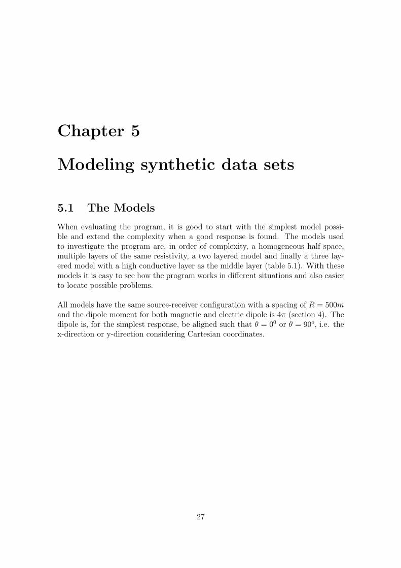
When evaluating the program, it is good to start with the simplest model possi-ble and extend the complexity when a good response is found. The models usedto investigate the program are, in order of complexity, a homogeneous half space,multiple layers of the same resistivity, a two layered model and finally a three lay-ered model with a high conductive layer as the middle layer (table 5.1). With thesemodels it is easy to see how the program works in different situations and also easierto locate possible problems.

All models have the same source-receiver configuration with a spacing of R = 500mand the dipole moment for both magnetic and electric dipole is 4π (section 4). Thedipole is, for the simplest response, be aligned such that θ = 00 or θ = 90o, i.e. thex-direction or y-direction considering Cartesian coordinates.

27

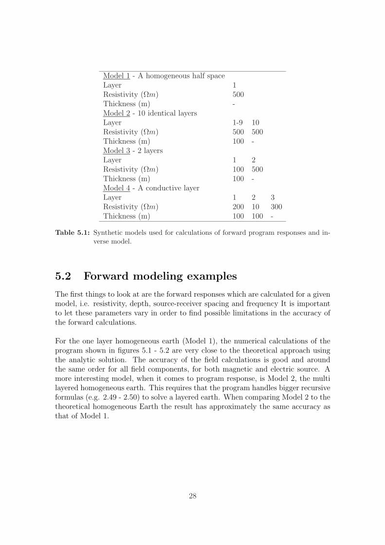
Model 1 - A homogeneous half spaceLayer 1Resistivity (Ωm) 500Thickness (m) -Model 2 - 10 identical layersLayer 1-9 10Resistivity (Ωm) 500 500Thickness (m) 100 -Model 3 - 2 layersLayer 1 2Resistivity (Ωm) 100 500Thickness (m) 100 -Model 4 - A conductive layerLayer 1 2 3Resistivity (Ωm) 200 10 300Thickness (m) 100 100 -

Table 5.1: Synthetic models used for calculations of forward program responses and in-verse model.

5.2 Forward modeling examples

The first things to look at are the forward responses which are calculated for a givenmodel, i.e. resistivity, depth, source-receiver spacing and frequency It is importantto let these parameters vary in order to find possible limitations in the accuracy ofthe forward calculations.

For the one layer homogeneous earth (Model 1), the numerical calculations of theprogram shown in figures 5.1 - 5.2 are very close to the theoretical approach usingthe analytic solution. The accuracy of the field calculations is good and aroundthe same order for all field components, for both magnetic and electric source. Amore interesting model, when it comes to program response, is Model 2, the multilayered homogeneous earth. This requires that the program handles bigger recursiveformulas (e.g. 2.49 - 2.50) to solve a layered earth. When comparing Model 2 to thetheoretical homogeneous Earth the result has approximately the same accuracy asthat of Model 1.

28

10−4

10−3

10−2

10−1

100

0.5

1

1.5

2x 10

−8

[H/m

]

Period [s]

Real Hφ

Forward responseTheoretical field

10−4

10−3

10−2

10−1

100

10−25

10−20

10−15

10−10

Period [s]

[H/m

]

Absolute difference

Figure 5.1: Real part of Hφ and difference between program response and analytic solu-tion of a magnetic dipole source over a homogeneous half space model, whereR = 500m, θ = 90o and ρ = 500Ωm.

10−4

10−3

10−2

10−1

100

0

1

2

3

4x 10

−9

[H/m

]

Period [s]

Imaginary Hφ


10−4

10−3

10−2

10−1

100

10−25

10−20

10−15

10−10

Period [s]

[H/m

]

Absolute difference

Figure 5.2: Imaginary part of Hφ and difference between program response and analyticsolution of a magnetic dipole source over a homogeneous half space model,where R = 500m, θ = 90o and ρ = 500Ωm.

There is only one deviation seen in the Model 1 forward response and that is in thecase of an electric dipole using high values of R and high frequencies. This showsthat there exists a frequency dependence that creates a major deviation of the

29

imaginary components of the E-field. For e.g. R = 10 km this is seen at frequencieshigher than around 10 kHz (figures 5.3 and 5.4). Since the Er-component has acos(θ) dependence and the Eφ-component has a sin(θ) dependence, these are givenat θ = 0o and θ = 90o respectively.

10−4

10−2

100

102

−4

−2

0

2x 10

−11 Imaginary Er[V

/m]

Period [s]


10−4

10−2

100

102

10−20

10−15

10−10

10−5

Period [s]

[V/m

]

Absolute difference

Figure 5.3: The imaginary component of Er and difference between program responseand theory for an electric dipole over a homogeneous half space model, wheresource-receiver distance is 10 km, θ = 0o and resistivity 500Ωm.

10−4

10−2

100

102

−2

0

2

4

6x 10

−11 Imaginary Eφ

[V/m

]

Period [s]


10−4

10−2

100

102

10−20

10−15

10−10

10−5

Period [s]

[V/m

]

Absolute difference

Figure 5.4: The imaginary component of Eφ and difference between program responseand theory for an electric dipole over a homogeneous half space model, wheresource-receiver distance is 10 km, θ = 90o and resistivity 500Ωm.

As seen, the dependence is caused by the imaginary part which has different signsfor Er and Eφ. This leads to the problem which lies in the two first components ofthe E-fields of a magnetic dipole (table 2.10) i.e. the kernel integral T1 (table 2.9).

30

This is most likely an effect of the discretization made for numerical integrations ofthe Bessel functions and as long as the same numeric tables for filter coefficients areused this deviation will remain.

For real applications the distance R varies depending on the resistivity but when itcomes to actual measurements this can probably be narrowed down to around 1 kmand with the frequencies the CSAMT method use this deviation will be neglectable.This means that for the used frequency range and the limit of R the program calcu-lations can be used only keeping this possible influence in mind when interpretingfurther models.

5.3 Sensitivity computation examples

Looking at the sensitivities is another way of making sure the program behaves inthe right way. These show the data dependence on model parameters and thereforedifferent for every parameter. As an example the, perturbation method sensitivities,derived with respect to the resistivities, can be observed. Figures 5.5 and 5.6 showthat these model parameters have a decreasing amplitude with frequency. Sincethe resistivity is the same for all cases, the figures show, for this resistivity, whichfrequencies that are best fit to model a given depth. The semi-analytical solution isthough not yet working so the perturbation method is used as standard.

10−5

10−4

10−3

10−2

10−1

100

−0.2

−0.1

0

0.1

0.2

ρ3

Period [s]10

−510

−410

−310

−210

−110

0

−0.02

0

0.02

ρ5

Period [s]

10−5

10−4

10−3

10−2

10−1

100

−5

0

5

x 10−3 ρ7

Period [s]10

−510

−410

−310

−210

−110

0

−2

−1

0

1

2

x 10−3 ρ9

Period [s]

Figure 5.5: Real part of sensitivities calculated using the perturbation method. Theimage show derivatives of Zrφ with respect to model parameters, ρ3, ρ5, ρ7

and ρ9. Model 2 is used for a magnetic dipole source.

31

10−5

10−4

10−3

10−2

10−1

100

−0.5

0

0.5ρ3

Period [s]10

−510

−410

−310

−210

−110

0

−0.1−0.05

00.050.1

ρ5

Period [s]

10−5

10−4

10−3

10−2

10−1

100

−0.05

0

0.05ρ7

Period [s]10

−510

−410

−310

−210

−110

0−0.02

−0.01

0

0.01

0.02ρ9

Period [s]

Figure 5.6: Real part of sensitivities calculated using the perturbation method. Theimage show derivatives of Zφr with respect to model parameters, ρ3, ρ5, ρ7

and ρ9. Model 2 is used for an electric dipole source.

5.4 Inverse modeling examples

When looking on the final program output, synthetic data have been used. To getdata sets that suit the program the same field calculations has been used to makesynthetic data for models of multiple layers. Also the discretization and filtering arethe same. For homogeneous half spaces, analytic solutions (Weidelt (1986) Table 1.3,p.80) are used which are based on the modified Bessel functions, I and K (equation2.53 - 2.54). To test the accuracy of the program it is best to start by using sets ofsynthetic input data without any noise or distortion. The result is shown in figure5.7 and 5.8. The angle θ has, for these figure, not been considered as discussed insection 4.

32

10−5

10−4

10−3

10−2

10−1

100

0

5

10

Zrφ

Period [s]10

−510

−410

−310

−210

−110

0−15

−10

−5

0

Period [s]

Zφ

r

10−5

10−4

10−3

10−2

10−1

100

−1

−0.5

0

0.5

Period [s]

A

Real part

Imaginary part

Figure 5.7: Synthetic data computed for Model 1 (table 5.1) with an electric dipoleconfiguration. The figures show the off-diagonal impedance components,Zrφ and Zφr, and the first tipper component A.

10−5

10−4

10−3

10−2

10−1

100

0

1

2

3

4

5

Zrφ

Period [s]10

−510

−410

−310

−210

−110

0−10

−5

0

Period [s]

Zφ

r

10−5

10−4

10−3

10−2

10−1

100

−0.4

−0.2

0

0.2

Period [s]

A

Real partImaginary part

Figure 5.8: Synthetic data computed for Model 1 (table 5.1) with a magnetic dipoleconfiguration. The figures show the off-diagonal impedance components,Zrφ and Zφr , and the first tipper component A.

The homogeneous earth model is the simplest case for the program to handle. Yetthere are some difficulties when letting the starting model deviate too much fromthe true model. There is also a frequency related problem that changes convergence

33

of the model when using too high frequencies. The frequency band used contains of29 frequencies increasing exponentially from 1 Hz to 31 kHz.

When using the whole frequency span, 1 Hz - 31 kHz, the model converge to apoint far from the true value and while step by step lowering the frequency span themodel convergence improves. Table 5.2 and 5.3 show the difference in convergencefor different frequencies and dipoles. The minimum frequency is always 1 Hz andthe model used here is Model 1.

Input [Ωm] Output [Ωm] NIT Fit fmax [Hz]500 254 9 7.06 31000.0500 432 4 3.56 9897.0500 478 4 1.73 1998.0500 496 3 0.83 493.0500 498.76 2 0.36 99.01000 498.76 5 0.36 99.0

Table 5.2: Model convergence for different frequency configurations. fmax is the maxi-mum frequency used and NIT is the number of iterations, where 201 is themaximum number. The synthetic data for Model 1, for an electric dipole, wasused. Fit is the data misfit (4.1), denoted Q2min in the program.

Input [Ωm] Output [Ωm] NIT Fit fmax [Hz]500 2949 Max 4.36 31000.0500 4369 15 2.71 9897.0500 1595 7 1.0 1998.0500 610 31 0.06 493.0500 553 15 0.0005 99.01000 559 8 0.0005 99.0

Table 5.3: Model convergence for the same configuration as table 5.2. The calculationsare made with Model 1 for a magnetic dipole.

To find convergence, fixed distortion parameters equal to zero are used for 5.2 whilefree floating, i.e. changing through the algorithm, distortion parameters are usedfor table 5.3. The magnetic dipole calculations also requires a different step size∆p to converge in the right direction for higher Fmax than 493 Hz. This is set to0.003 which was three times the value used for the electric dipole. After loweringthe frequencies to Fmax = 99Hz the step size can again be reduced to get a betterresult (input: 500 Ωm → ouput: 525 Ωm) than in table 5.3.

34

Even though some convergence is found, it is still strange that the iteration startseven though the starting model is the true model. The synthetic data does notdeviate from the program field calculations, since they are calculated in the exactsame way.

The program also has some input model limitations e.g. problems in convergencefor much deviating models. These changes for different frequencies and for lowerfrequencies the program can handle more deviating models. The last measurementsin table 5.2 and 5.3 are the most trustworthy but the noise, standard deviation androtation are here set to zero. To get a more complete picture two more tests (5.4)are made where the input data include a standard deviation and noise of 5%. Thenoise is gaussian and added or subtracted from the impedance and tipper when thesynthetic data is made.

Dipole Input [Ωm] Output [Ωm] NIT Fit fmax [Hz]E 1000 499.26 5 0.41 99.0M 1000 526 16 0.0005 99.0

Table 5.4: Output using noisy input data for electric (E) and magnetic (M) dipole sourceof Model 1.

The result deviates a little bit but is still stable. One might though question thelow accuracy result of the magnetic dipole. Model 2, the ten layered model, requiressome changes in input values to get some convergence but this show no good resultand is very sensitive to changes in the input model. The output for Model 2, withthe true model as input, is given in figure 5.9 and 5.10.

When using Model 3, one expects to really see how well the program works and towhat range or depth the calculations hold. Table 5.5 shows that the result is notvery good and it is uncertain if, what might looks like convergence, is true or onlycoincidence. For even more deviating input models, the program will not show anyconnection with the true model.

Dipole Input (ρ1, ρ2, d1) Output NIT Fit fmax [Hz]E 100, 500, 100 105, 680, 90 6 0.16 99.0E 150, 580, 70 138, 575, 74 2 0.46 99.0M 100, 500, 100 104, 496, 104 2 0.008 99.0M 150, 580, 70 95, 433, 96 27 0.008 99.0

Table 5.5: Model convergence for Model 3 for both electric (E) and magnetic (M) dipolesource.

35

−200

0

200

400

600

800

1000

Dep

th(m

)

Model convergence of Model 2 using an electric dipole configuration

400 500 600

−200

0

200

400

600

800

1000

Resistivity (Ωm)

Dep

th(m

)

Starting modelCalculated model


Figure 5.9: Model 2 found by program where the input is the true model. The picturesshow deviation from the true thickness (left picture) and deviation from trueresistivity (right picture). An electric dipole configuration is used. The thickrugged line represents the Earth’s surface.

−200

0

200

400

600

800

1000

Dep

th(m

)

Model convergence of Model 2 using a magnetic dipole configuration

0 500 1000

−200

0

200

400

600

800

1000

Resistivity (Ωm)

Dep

th(m

)



Figure 5.10: Model 2 found by program where the input is the true model. The picturesshow deviation from the true thickness (left picture) and deviation fromtrue resistivity (right picture). A magnetic dipole configuration is used.The thick rugged line represents the Earth’s surface.

36

Chapter 6

Program response

6.1 Comparing the response with an X3D pro-

gram

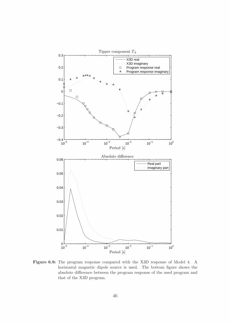
To really know the accuracy of the program response it is good to compare theprogram response with some professional modeling e.g. the X3D program base onthe publication by Avdeev et al. (2002). Images of the response of Model 1 (figure6.1-6.3), Model 3 (figure 6.4-6.6) and Model 4 (figure 6.7-6.9) show that an increasedmodel complexity decreases the accuracy if the X3D program is assumed to be thetrue response.

The biggest differences are seen in the high frequency area. For Model 4, it is veryclear that the program fails at high frequencies. The deviation of the calculatedmodel to the X3D model can, in the worst cases, be almost 100 %. In Model 4 thereare also some deviations around the lower frequencies in e.g. tipper component TA

in figure 6.6. For frequencies lower than around 100 Hz the deviation rarely is morethan 10 % and for Model 1 the deviation is in general less than 1 %.

37

10−5

10−4

10−3

10−2

10−1

100

−2

0

2

4

6

8

10

12

14

16

Period [s]

Impedance component Zrφ

X3D realX3D imaginaryProgram response realProgram response imaginary

10−5

10−4

10−3

10−2

10−1

100

0

0.01

0.02

0.03

0.04

0.05

0.06

0.07

0.08

0.09

0.1Absolute difference

Period [s]


Figure 6.1: The program response compared with the X3D response of Model 1. A hor-izontal electric dipole source is used. The bottom figure shows the absolutedifference between the program response of the used program and that ofthe X3D program.

38

10−5

10−4

10−3

10−2

10−1

100

−16

−14

−12

−10

−8

−6

−4

−2

0

2

Period [s]

Impedance component Zφr


10−5

10−4

10−3

10−2

10−1

100

0

0.005

0.01

0.015

0.02

0.025


Period [s]


Figure 6.2: The program response compared with the X3D response of Model 1. Ahorizontal magnetic dipole source is used. The bottom figure shows theabsolute difference between the program response of the used program andthat of the X3D program.

39

10−5

10−4

10−3

10−2

10−1

100

−0.4

−0.3

−0.2

−0.1

0

0.1

0.2

0.3Tipper component TA

Period [s]


10−5

10−4

10−3

10−2

10−1

100

0

0.002

0.004

0.006

0.008

0.01

0.012

0.014

0.016

0.018


Period [s]



40

10−5

10−4

10−3

10−2

10−1

100

−1

0

1

2

3

4

5

6

7

Period [s]



10−5

10−4

10−3

10−2

10−1

100

0

0.2

0.4

0.6

0.8

1

1.2


Period [s]



41

10−5

10−4

10−3

10−2

10−1

100

−8

−7

−6

−5

−4

−3

−2

−1

0

1

Period [s]



10−5

10−4

10−3

10−2

10−1

100

0

0.1

0.2

0.3

0.4

0.5

0.6

0.7

0.8


Period [s]



42

10−5

10−4

10−3

10−2

10−1

100

−0.5

−0.4

−0.3

−0.2

−0.1

0

0.1


Period [s]


10−5

10−4

10−3

10−2

10−1

100

0

1

2

3

4

5

6

7

8

9x 10

−3 Absolute difference

Period [s]



43

10−5

10−4

10−3

10−2

10−1

100

0

2

4

6

8

10

12

Period [s]



10−5

10−4

10−3

10−2

10−1

100

0

0.5

1

1.5

2

2.5

3

3.5

4

4.5

5Absolute difference

Period [s]



44

10−5

10−4

10−3

10−2

10−1

100

−9

−8

−7

−6

−5

−4

−3

−2

−1

0

1

Period [s]



10−5

10−4

10−3

10−2

10−1

100

0

0.5

1

1.5

2

2.5

3

3.5

4


Period [s]



45

10−5

10−4

10−3

10−2

10−1

100

−0.4

−0.3

−0.2

−0.1

0

0.1

0.2


Period [s]


10−5

10−4

10−3

10−2

10−1

100

0

0.01

0.02

0.03

0.04

0.05


Period [s]



46

Chapter 7

Process and result

7.1 Implementing a magnetic dipole source

The old program was not up to date and strictly used for an electric dipole source.By adding a choice of using a magnetic dipole followed by other improvements theprogram can be more versatile and hence more useful. The magnetic/electric dipoleis now set up as a choice made by the user input and the selection is made forthe field calculations and not integrals or kernels. The calculations follows Weidelt(1986) (table 2.10) for z ≈ 0. An exception is in the Electric field components thatcontain a sign(z+). Since z only is approximated to zero, and really positive, thisset to +1.

When looking at the comparison done with the X3D program in chapter 6 theresponse looks rather satisfying for Model 1, where the deviation is less than 1 % forTA which has up to 10 % at high frequencies. For Model 3 and Model 4 the deviationcan reach up to extreme numbers such as close to 100 % for some components athigh frequencies. In total it is not this bad and for frequencies under 100 Hz thedeviation is lower than 10 % for all cases.

7.2 Improving sensitivities

In the previous program version the sensitivity calculations had been set up for bothmethods but the Newtonian approach was used as standard. To be able to use thenumerical procedure, the derivatives of the integral kernels had to be rewritten aswell as adding the field sensitivity calculations for a magnetic dipole source. Asthe field calculations are done through exactly the same numerical procedure thisapproach requires no approximation hence is more exact.

This method is however not used at the moment. The problem is that even thoughthe sensitivities frequency dependence is good, the magnitude of the sensitivity is in-correct. This can, hopefully, be corrected very quickly once the algorithm has been

47

looked through. One advantage with the perturbation method is that it requiresless work, both for the programmer and the program and it is, for simpler models,therefore more reasonable to use.

Another correction made here was to change the sensitivity calculations due to thedependence on the logarithmic model parameters, resistivity and depth. In theanalytical approach of the sensitivity calculations this had been overlooked in someplaces and an additional factor had to be used because of the derivation of thenatural logarithm (equation 7.1).

∂di

∂log(pj)=

∂di

∂log(pj)

∂pj

∂pj

=∂di

∂pj

(∂log(pj)

∂pj

)−1

=∂di

∂pj

pj (7.1)

The semi-analytically derived sensitivities are though still not correct. The out-put is many magnitudes too big. This is a problem in the derivatives of the fieldcomponents. As an example the model for an electric dipole configuration over ahomogeneous half space can converge very good if the derivatives are multiplied byapproximately 2 · 10−9. This is somewhat in the order of what differs the differentsensitivity approaches. By this it is clear that there are some errors in the calcu-lations of the analytical sensitivities. Since, at least, frequency dependence of thesensitivities is correct there is a good chance this is solved very quickly.

48

Chapter 8

Conclusions & Further work

The summary so far is that more work has to be put into the inversion and theLevenberg-Marquardt algorithm. This conclusion can be drawn from the fact thatthe simplest of models will converge only under some conditions, e.g. limits in inputmodel or frequency, while models that are more advanced than a homogeneous halfspace give erroneous output.

The program does not show any consistent convergence for Model 2, Model 3 andModel 4 at all. Only when the true model is put in as the starting model one mightbe so lucky as to have a nice answer. My main goal was to implement the magneticdipole configuration. This was made successfully but it has in the end turned out tobe the rest of the program, e.g. the sensitivities, inversion algorithm and damping,that needs to be improved or repaired. To get the program to work time should beput on the algorithm alone.

The sensitivities might be a little too simple but with some modifications these canbe improved. The analytical solutions of the sensitivities are almost usable and withanother thoroughly check these will surely be working properly.

Finally there might be some thoughts about the program usability and if it reallyis worth putting more energy on getting it fully functional. At the moment the nu-merical field calculations are very good and in no need to be changed. The programitself is, in many situations, very useful to get a quick and simple view of the sub-surface structure. The result is good to compare with other, professional, modelingprograms or just to find out if the measurement is worth further examination. It ismy hope that this report can be a help for future studies of this program.

49

Fig

ure

8.1:

Pro

gram

tree

over

mai

npr

ogra

m,m

odul

es,su

brou

tine

san

dfu

ncti

ons.

Bibliography

Arfken, G. B. and Weber, H. J. (2005). Mathematical Methods for Physicists. Else-vier Academic Press.

Aster, R. C., Borchers, B., and Thurber, C. H. (2005). Parameter estimation andinverse problems. Elsevier Academic Press.

Avdeev, D., Kuvshinov., A., Pankratov, O., and Newman, G. (2002). Three-dimensional induction logging problems, part i an integral equation solution andmodel comparisons. Geophysics, 67:413–426.

Bastani, M. (2001). EnviroMT - a New Controlled Source/Radio MagnetotelluricSystem. PhD thesis, Uppsala Universitet.

Garcia, X., Boerner, D., and Pedersen, L. B. (2003). Electric and magnetic gal-vanic distortion decomposition of tensor csamt data. application to data fromthe buchans mine (newfoundland, canada). Geophysical Journal International,154(3):957–969.

Hjarten, M. (2007). Master thesis in interpretation of controlled-source radiomag-netotelluric data from Hallandsasen. Master’s thesis, Uppsala Universitet.

Li, X. and Pedersen, L. B. (1991). Controlled source tensor magnetotellurics. Geo-physical Journal International, 56(9):1456–1461.

Menke, W. (1989). Geophysical Data Analysis: Discrete Inverse Theory. AcademicPress, Inc., New York.

Pedersen, L. B. and Rasmussen, T. M. (1989). Inversion of magnetotelluric data: Anon-linear least-squares approach. Geophysical Prospecting, 37(6):669–695.

Ward, S. H. and Hohmann, G. W. (1988). Electromagnetic theory for geophysicalapplication. In Electromagnetic Methods in Applied Geophysics, ed. Nabighian M.Soc. Expl. Geophys., Tulsa.

Weidelt, P. (1986). Einfuhrung in die elektromagnetische Tiefenforschung. Vor-lesungsskript, Technische Universitat Braunschweig, Braunschweig.

51

Zhang, P., Roberts, R. G., and Pedersen, L. B. (1987). Magnetotelluric strike rules.Geophysical Journal International, 52(3):267–278.

Zonge, K. L. and Hughes, L. J. (1991). Controlled source audio-frequency magne-totellurics. In Electromagnetic Methods in Applied Geophysics, ed. Nabighian M.Soc. Expl. Geophys., Tulsa.

52

A note on electromagnetic ﬂeld theory and 1D modeling of ...564462/FULLTEXT01.pdf · A note on...

Documents

Transcript of A note on electromagnetic ﬂeld theory and 1D modeling of ...564462/FULLTEXT01.pdf · A note on...