A nonparametric wet/dry spell model for resampling daily precipitation
21
A nonparametric wet/dry spell model for resampling daily precipitation Upmanu Lall Department of Civil and Environmental Engineering and Utah Water Research Laboratory, Utah State University, Logan Balaji Rajagopalan Lamont-Doherty Earth Observatory of Columbia University, Palisades, New York David G. Tarboton Department of Civil and Environmental Engineering and Utah Water Research Laboratory, Utah State University, Logan Abstract. A nonparametric wet/dry spell model is developed for resampling daily precipitation at a site. The model considers alternating sequences of wet and dry days in a given season of the year. All marginal, joint, and conditional probability densities of interest (e.g., dry spell length, wet spell length, precipitation amount, and wet spell length given prior to dry spell length) are estimated nonparametrically using at-site data and kernel probability density estimators. Procedures for the disaggregation of wet spell precipitation into daily precipitation and for the generation of synthetic sequences are proffered. An application of the model for generating synthetic precipitation traces at a site in Utah is presented. 1. Introduction Synthetically generated sequences of daily precipitation are often used for investigating likely scenarios for agricultural water requirements, reservoir operation for analyses of ante- cedent moisture conditions, and runoff generation in a water- shed. Preserving the characteristics of multiday wet and dry spells is often important in these applications. This paper pre- sents a stochastic model for resampling daily precipitation where the probability distributions functions (pdf’s) of alter- nating wet and dry spell lengths and of rainfall amount are estimated nonparametrically using kernel density estimators. This procedure is equivalent to a bootstrap or sampling with replacement of the observed data sequence of spell lengths and precipitation amounts. It differs from the classical bootstrap in that smoothed rather than empirical distribution functions are used for resampling, and sequential attributes of spells may be preserved. Necessary calibration parameters are chosen auto- matically from the data set using measures aimed at providing a good fit to the unknown underlying pdf. Our particular interest was in developing a scheme for syn- thetic simulation of daily precipitation in mountainous regions in the western United States. Precipitation in these areas is in the form of snow in the winter with orographic and frontal mechanisms dominant. Convective rainfall processes occur in other seasons. Marked differences in the storm tracks and moisture sources over the seasons are observed. A mixture of markedly different mechanisms (some related to the El Nino- Southern Oscillation) leads to the precipitation process in the western United States [Webb and Bettencourt, 1992; Cayan and Riddle, 1992]. Recognition of such heterogeneities has led to efforts at regime identification and modeling of rainfall condi- tional on weather types [e.g., Katz and Parlange, 1993; Wilson and Lettenmeier, 1993; Bogardi et al., 1993]. While this is an attractive and necessary approach, deconvolution of mixtures is not always easy from a finite data set and the weather type designations used can be subjective. Traditionally, parametric probability models (e.g., exponential distribution), whose func- tional form is completely specified by a small set of parameters are used to fit the relevant frequency distributions. Selecting the best such model is tenuous [see Vogel and McMartin, 1991] even where mixtures are not of concern. The work presented here was motivated by the following questions: 1. Is it possible to resample the data while preserving the relative frequencies and conditional relative frequencies of wet and dry spells and precipitation amounts without prior assump- tions as to the parametric forms of the underlying probability models? 2. What is a good way to empirically model the relevant pdf for resampling and to guide development of statistical models? 3. Can such a data-based assessment of probabilities or relative frequencies be used to judge the adequacy of concep- tual and statistical models posed for daily rainfall? The first question is relevant not only from a conceptual standpoint but also because organizations (e.g., U.S. Forest Service, U.S. Department of Agriculture) specify a uniform procedure for applications from site to site, where parametric distributions or procedures are used, “models” that work well in some regions/sites fail at others. In our view it is unlikely that a robust parametric framework for model specification and selection can be devised for uniform application given the likely heterogeneity in precipitation generation mechanisms. Copyright 1996 by the American Geophysical Union. Paper number 96WR00565. 0043-1397/96/96WR-00565$09.00 WATER RESOURCES RESEARCH, VOL. 32, NO. 9, PAGES 2803–2823, SEPTEMBER 1996 2803
-
Upload
truongthuy -
Category
Documents
-
view
217 -
download
0
Transcript of A nonparametric wet/dry spell model for resampling daily precipitation

A nonparametric wet/dry spell model for resampling dailyprecipitation
Upmanu LallDepartment of Civil and Environmental Engineering and Utah Water Research Laboratory, Utah StateUniversity, Logan
Balaji RajagopalanLamont-Doherty Earth Observatory of Columbia University, Palisades, New York
David G. TarbotonDepartment of Civil and Environmental Engineering and Utah Water Research Laboratory, Utah StateUniversity, Logan
Abstract. A nonparametric wet/dry spell model is developed for resampling dailyprecipitation at a site. The model considers alternating sequences of wet and dry days in agiven season of the year. All marginal, joint, and conditional probability densities ofinterest (e.g., dry spell length, wet spell length, precipitation amount, and wet spell lengthgiven prior to dry spell length) are estimated nonparametrically using at-site data andkernel probability density estimators. Procedures for the disaggregation of wet spellprecipitation into daily precipitation and for the generation of synthetic sequences areproffered. An application of the model for generating synthetic precipitation traces at asite in Utah is presented.
1. IntroductionSynthetically generated sequences of daily precipitation are
often used for investigating likely scenarios for agriculturalwater requirements, reservoir operation for analyses of ante-cedent moisture conditions, and runoff generation in a water-shed. Preserving the characteristics of multiday wet and dryspells is often important in these applications. This paper pre-sents a stochastic model for resampling daily precipitationwhere the probability distributions functions (pdf’s) of alter-nating wet and dry spell lengths and of rainfall amount areestimated nonparametrically using kernel density estimators.This procedure is equivalent to a bootstrap or sampling withreplacement of the observed data sequence of spell lengths andprecipitation amounts. It differs from the classical bootstrap inthat smoothed rather than empirical distribution functions areused for resampling, and sequential attributes of spells may bepreserved. Necessary calibration parameters are chosen auto-matically from the data set using measures aimed at providinga good fit to the unknown underlying pdf.Our particular interest was in developing a scheme for syn-
thetic simulation of daily precipitation in mountainous regionsin the western United States. Precipitation in these areas is inthe form of snow in the winter with orographic and frontalmechanisms dominant. Convective rainfall processes occur inother seasons. Marked differences in the storm tracks andmoisture sources over the seasons are observed. A mixture ofmarkedly different mechanisms (some related to the El Nino-Southern Oscillation) leads to the precipitation process in thewestern United States [Webb and Bettencourt, 1992; Cayan andRiddle, 1992]. Recognition of such heterogeneities has led to
efforts at regime identification and modeling of rainfall condi-tional on weather types [e.g., Katz and Parlange, 1993; Wilsonand Lettenmeier, 1993; Bogardi et al., 1993]. While this is anattractive and necessary approach, deconvolution of mixturesis not always easy from a finite data set and the weather typedesignations used can be subjective. Traditionally, parametricprobability models (e.g., exponential distribution), whose func-tional form is completely specified by a small set of parametersare used to fit the relevant frequency distributions. Selectingthe best such model is tenuous [see Vogel and McMartin, 1991]even where mixtures are not of concern.The work presented here was motivated by the following
questions:1. Is it possible to resample the data while preserving the
relative frequencies and conditional relative frequencies of wetand dry spells and precipitation amounts without prior assump-tions as to the parametric forms of the underlying probabilitymodels?2. What is a good way to empirically model the relevant
pdf for resampling and to guide development of statisticalmodels?3. Can such a data-based assessment of probabilities or
relative frequencies be used to judge the adequacy of concep-tual and statistical models posed for daily rainfall?The first question is relevant not only from a conceptual
standpoint but also because organizations (e.g., U.S. ForestService, U.S. Department of Agriculture) specify a uniformprocedure for applications from site to site, where parametricdistributions or procedures are used, “models” that work wellin some regions/sites fail at others. In our view it is unlikelythat a robust parametric framework for model specificationand selection can be devised for uniform application given thelikely heterogeneity in precipitation generation mechanisms.
Copyright 1996 by the American Geophysical Union.
Paper number 96WR00565.0043-1397/96/96WR-00565$09.00
WATER RESOURCES RESEARCH, VOL. 32, NO. 9, PAGES 2803–2823, SEPTEMBER 1996
2803

Here we sidestep such issues by using a resampling strategythat honors at-site data directly.The second question is addressed in paper by B. Rajago-
palan et al. Evaluation of kernel density estimation methodsfor daily precipitation resampling, submitted to Stochastic Hy-drology and Hydraulics, 1995, hereinafter referred to as sub-mitted manuscript, 1995) where we document our investiga-tions into developing appropriate kernel density estimators forresampling continuous (e.g., precipitation amount) and dis-crete (e.g., spell length in days) random variables.With regards to the third question, we argue that the answer
is likely to be yes, given that the relevant probability densitiescan be estimated reliably from the data. However, this is anarea that we expect to research formally in the future anddiscuss only generally here.We begin with a brief review of available models for simu-
lating daily precipitation and an introduction to the centralideas in kernel density estimation. The nonparametric, alter-nating wet/dry spell model is presented next, and the resam-pling/simulation strategy is indicated. Results from an applica-tion to a Utah data set follow. The performance of thenonparametric scheme is compared with a simple, parametricalternative. A discussion of applicability, limitations of theapproach, and musings on pointers to related work in progressconcludes the presentation.
2. BackgroundReviews of stochastic precipitation models are offered by
Waymire and Gupta [1981a, b, c], Georgakakos and Kavvas[1987], and Foufoula-Georgiou and Georgakokas [1988]. Thereader is referred to these papers for an appreciation of theliterature and the central issues perceived in the field. Whilewe are aware of the need to look at the concurrent represen-tation of the precipitation process at different timescales, ourfocus here will only be on daily precipitation. Precipitationmodels have two components: (1) a model for precipitationoccurrence, usually formulated as a Markov process, and (2) amodel for precipitation amount, once a precipitation event hasbeen generated. In the latter case, typically a parsimoniousmember of the exponential family that best fits a given data setis used. A firm basis for such a choice has yet to emerge, andtypical tests for selecting between parametric distributions,such as the chi-square test, often lack the power to discriminatebetween different candidate distributions, since most of themass of the pdf is concentrated near the origin. This practice isalso questionable given our earlier comments that a mix ofgenerating processes likely governs precipitation. A brief dis-cussion of the attributes of some models for daily precipitationoccurrence follows.
2.1. Markov Chain Models
The most popular approach is to consider the precipitationoccurrence process to be described by a finite state (typically 2,a day is wet W or dry D) Markov Chain (MC) of finite order(typically 1), with seasonally (or time varying) transition prob-abilities. The basic assumption is that the present state (wet ordry) depends only on the immediate past. The transition prob-abilities for transitions (i.e., WW, WD, DW, DD) between thetwo states (W or D) are estimated directly from the datathrough a counting process. Fourier series methods [Feyerharmand Bark, 1965; Woolhiser et al., 1988] may be used to param-eterize seasonal variations in the transition probabilities. The
degree of dependence in time is limited by the order of theMC. Feyerharm and Bark [1967] and Chin [1977] suggest thatthe order may need to be seasonally variable as well. Lack ofparsimony is a drawback of MC models as the order is in-creased. A number of researchers [Hopkins and Robillard,1964; Haan et al., 1976; Srikanthan and McMahon, 1983; Guz-man and Torrez, 1985] have also stressed the need for multi-state MC models that consider the dependence between tran-sition probabilities and rainfall amount.Chang et al. [1984] and Foufoula-Georgiou and Georgakakos
[1988] argue that Markov Chain models do not reproduce longterm persistence and event clustering very readily. MarkovChain models can be attractive because of their largely non-parametric nature, ease of application and interpretability, andwell-developed literature. Wilson and Lettenmeier [1993] pur-sue a hierarchical MC model to describe the daily precipitationprocess given the heterogeneous generating mechanisms prev-alent in the western United States. While this approach ad-dresses the heterogeneity issue, the relative lack of parsimonyand shortcomings of the MC model identified above detractfrom the formulation.
2.2. Wet-Dry Spell Approach
In probabilistic terminology, this approach is also called thealternating renewal model (ARM). The term renewal stemsfrom the implied independence between the dry and wet pe-riod length, while the term alternating refers to the fact thatwet and dry states alternate. No transition to the same state ispossible. An advantage of this representation is that it allowsdirect consideration of a composite precipitation event, ratherthan its discontinuous truncation into arbitrary daily segments.A geometric or a negative binomial distribution [Roldan and
Woolhiser, 1982] may be used as a model for spell length, wherea daily time step is of interest. A probability distribution forwet spell precipitation amount also needs to be developed, asdoes a procedure for the disaggregation of wet spell precipi-tation to daily precipitation, for wet spells that are longer thanone day.The primary difficulties cited with the wet/dry spell approach
for daily rainfall modeling are (1) the need for disaggregationof wet spell precipitation into daily or event precipitation (thisis not an issue if independence in daily precipitation amountsis assumed, since that is typically assumed by Markov Chainmodels), (2) the justification of the independence between thedry and wet spell lengths at short timescales, and (3) the ef-fective reduction in the sample size by considering spells ratherthan days. We also find the usual parametric specifications forprobability distributions and assumptions of independence ofspells in such models objectionable in light of the likely heter-ogeneous nature of the data of interest to us. However, we dofind this structure plausible and address some of the difficultiescited here in our development.
3. Model FormulationFor the nonparametric, seasonal wet/dry spell (NSS) model
presented here, the random variables of interest are the wetspell length w (days), dry spell length d (days), daily precipi-tation amount p (inches), and the wet spell precipitationamount pw (inches). Note that throughout the paper, wet dayprecipitation is referred to as daily precipitation. Variables wand d are defined through the set of integers greater than 1(and less than season length), and p and pw are defined as
LALL ET AL.: NONPARAMETRIC WET/DRY SPELL MODEL2804

continuous, positive (actually greater than a measurementthreshold, e.g., 0.01 inches rather than 0) random variables. Amixed set of discrete and continuous random variables is thusconsidered. Appropriate season definitions are prescribed bythe model user, and model definitions that follow pertain to agiven season of the year. The natural sequence of seasons ismaintained, and spells in progress at the end of a season areallowed to terminate in the succeeding season.The general structure of the model is similar to that of a
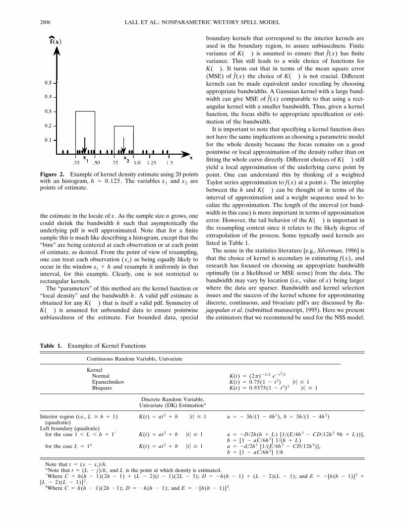
wet/dry spell model. Our model differs from the traditionalwet/dry spell model in a number of ways, as illustrated inFigure 1. The dry and wet spell lengths in a season may bedependent. The data are allowed to indicate whether such anassumption is necessary. Rather than fitting parametric prob-ability densities to the data, we consider kernel estimators ofthe probability mass/density function (pmf/pdf) of wet spelllength f(w), dry spell length f(d), wet day precipitationamount f( p), wet spell precipitation amount f( pw), the jointpmf of wet and dry spell length f(w, d), the joint pdf of wetspell length and wet spell precipitation f(w, pw), and theconditional pdf of wet spell length given dry spell lengthf(w ud), dry spell length given wet spell length f(d uw), and wetspell precipitation given wet spell length f( pwuw).First, the significance of the dependence between successive
wet and dry spell lengths is assessed by computing their samplecorrelation for each season. The precipitation occurrence pro-cess in a given season is described through the conditionalpmf’s f(w ud) and f(d uw) if the correlation is significant and themarginal pmf’s f(w) and f(d) otherwise. The latter with para-metrically specified pmf corresponds to the traditional alter-nating renewal model. The former is a more general depen-dence structure. Next, one estimates for each season theautocorrelation function for precipitation amounts pi, i 51, z z z , w for each spell length. If these correlations are notsignificant, it is assumed that there is no “statistical structure”in the within spell precipitation, at least for daily precipitationamounts. In this case, daily precipitation is modeled directlythrough an estimate of the pdf f( p). If there is evidence forstructure in wet spell precipitation, wet spell precipitation pwbecomes the primary variable, and a disaggregation approachthat preserves the within spell structure is used to disaggregatepw to daily precipitation amounts. In most applications usingtraditional wet/dry spell models or the one presented here, thedisaggregation approach is eschewed in favor of treating dailyprecipitation as an independent random variable.The decisions on model structure as well as the relevant pdf
for each variable for each season are different and are inde-pendently estimated. To save on notation, we have chosen notto index any of our variables by season. In summary, the pri-mary differences with the traditional wet/dry spell model arethe following: (1) the relevant probability functions are esti-mated without recourse to prior assumptions as to the para-metric form of the model, and (2) a more general conditionaldependence structure is admitted.We stress that while we are ultimately interested in devel-
oping a nonparametric model for generating daily precipita-tion sequences, the nonparametric density estimates generateden route are interesting since they reveal tendencies or struc-ture in the precipitation process. We now describe how the pdfand pmf are estimated. The univariate cases are discussed firstfollowed by the bivariate/conditional cases. The disaggregationapproach is finally presented.
3.1. Nonparametric Kernel Function Estimation
Nonparametric estimation of probability and regressionfunctions is an emerging area in stochastic hydrology. A reviewof recent applications is offered by Lall [1995]. A functionapproximation method is considered nonparametric if (1) it iscapable of approximating a large number of target functions,(2) it is “local” in that estimates of the target function at apoint use only observations located within some small neigh-borhood of the point, and (3) no prior assumptions are madeas to the overall functional form of the target function. Ahistogram is a familiar example of such a method. Such meth-ods do have parameters (e.g., the bin width of the histogram)that influence the estimate at a point. However, they are dif-ferent from “parametric” methods where the entire function isindexed by a finite set of parameters (e.g., mean and standarddeviation), and a prescribed functional form.Kernel density estimation is a nonparametric method of
estimating a pdf from data that is related to the histogram.Recent expository monographs that develop these ideas in-clude [Silverman, 1986; Scott, 1992; Hardle, 1991]. Given a setof observations x1, z z z , xn (in general x may be a scalar or avector), the kernel density estimate (kde) is defined as
f~ x! 51hn O
i51
n
KS x 2 xih D (1)
where K( ) is a weight or kernel function and h is a bandwidth.The idea is illustrated through Figure 2. Consider the defi-
nition of probability as a relative frequency of event occur-rence. Now an estimate of the probability density at a point x(refer to points x1 and x2 in Figure 1) may be obtained if weconsider a box or window of width 2h centered at x and countthe number of observations that fall in such a box. The esti-mate f( x) is then (number of xi that lie within [ x 2 h,x 1 h])/(2hn)). In this example, we have used a rectangularkernel (K(t) 5 1/ 2 for ut u , 1, 0 else; t 5 ( x 2 xi)/h) for
Figure 1. Structure of the wet/dry spell precipitation model.
2805LALL ET AL.: NONPARAMETRIC WET/DRY SPELL MODEL
the estimate in the locale of x. As the sample size n grows, onecould shrink the bandwidth h such that asymptotically theunderlying pdf is well approximated. Note that for a finitesample this is much like describing a histogram, except that the“bins” are being centered at each observation or at each pointof estimate, as desired. From the point of view of resampling,one can treat each observation ( xi) as being equally likely tooccur in the window xi 1 h and resample it uniformly in thatinterval, for this example. Clearly, one is not restricted torectangular kernels.The “parameters” of this method are the kernel function or
“local density” and the bandwidth h. A valid pdf estimate isobtained for any K( ) that is itself a valid pdf. Symmetry ofK( ) is assumed for unbounded data to ensure pointwiseunbiasedness of the estimate. For bounded data, special
boundary kernels that correspond to the interior kernels areused in the boundary region, to assure unbiasedness. Finitevariance of K( ) is assumed to ensure that f( x) has finitevariance. This still leads to a wide choice of functions forK( ). It turns out that in terms of the mean square error(MSE) of f( x) the choice of K( ) is not crucial. Differentkernels can be made equivalent under rescaling by choosingappropriate bandwidths. A Gaussian kernel with a large band-width can give MSE of f( x) comparable to that using a rect-angular kernel with a smaller bandwidth. Thus, given a kernelfunction, the focus shifts to appropriate specification or esti-mation of the bandwidth.It is important to note that specifying a kernel function does
not have the same implications as choosing a parametric modelfor the whole density because the focus remains on a goodpointwise or local approximation of the density rather than onfitting the whole curve directly. Different choices of K( ) stillyield a local approximation of the underlying curve point bypoint. One can understand this by thinking of a weightedTaylor series approximation to f( x) at a point x . The interplaybetween the h and K( ) can be thought of in terms of theinterval of approximation and a weight sequence used to lo-calize the approximation. The length of the interval (or band-width in this case) is more important in terms of approximationerror. However, the tail behavior of the K( ) is important inthe resampling context since it relates to the likely degree ofextrapolation of the process. Some typically used kernels arelisted in Table 1.The sense in the statistics literature [e.g., Silverman, 1986] is
that the choice of kernel is secondary in estimating f( x), andresearch has focused on choosing an appropriate bandwidthoptimally (in a likelihood or MSE sense) from the data. Thebandwidth may vary by location (i.e., value of x) being largerwhere the data are sparser. Bandwidth and kernel selectionissues and the success of the kernel scheme for approximatingdiscrete, continuous, and bivariate pdf’s are discussed by Ra-jagopalan et al. (submitted manuscript, 1995). Here we presentthe estimators that we recommend be used for the NSS model.
Figure 2. Example of kernel density estimate using 20 pointswith an histogram, h 5 0.125. The variables x1 and x2 arepoints of estimate.
Table 1. Examples of Kernel Functions
Continuous Random Variable, Univariate
KernelNormal K(t) 5 (2p)21/2 e2t2/2
Epanechnikov K(t) 5 0.75(1 2 t2) ut u # 1Bisquare K(t) 5 0.9375(1 2 t2)2 ut u # 1
Discrete Random Variable,Univariate (DK) Estimation*
Interior region (i.e., L $ h 1 1)(quadratic)
K(t) 5 at2 1 b ut u # 1 a 5 2 3h/(1 2 4h2), b 5 3h/(1 2 4h2)
Left boundary (quadratic)for the case 1 , L , h 1 1† K(t) 5 at2 1 b ut u # 1 a 5 2D/2h(h 1 L) [1/(E/4h3 2 CD/12h3 9h 1 L))],
b 5 [1 2 aC/6h2] 1/(h 1 L)for the case L 5 1‡ K(t) 5 at2 1 b ut u # 1 a 5 2d/2h2 [1/(E/4h3 2 CD/12h4)],
b 5 [1 2 aC/6h2] 1/h
Note that t 5 ( x 2 xi)/h.*Note that t 5 (L 2 j)/h, and L is the point at which density is estimated.†Where C 5 h(h 2 1)(2h 2 1) 1 (L 2 2)(i 2 1)(2L 2 3); D 5 2h(h 2 1) 1 (L 2 2)(L 2 1); and E 5 2[h(h 2 1)]2 1
[L 2 2)(L 2 1)]2.‡Where C 5 h(h 2 1)(2h 21); D 5 2h(h 2 1); and E 5 2[h(h 2 1)]2.
LALL ET AL.: NONPARAMETRIC WET/DRY SPELL MODEL2806
3.2. Kernel Estimation of Continuous, Univariate pdf’s
The continuous, univariate pdf’s of interest to us are f( p),the pdf of daily precipitation, and f( pw), the pdf of wet spellprecipitation for a season. The data set in the first case iscomposed of np days of daily precipitation values, pi, for alldays with measurable precipitation, in season s for the y yearrecord. For pw the data set is composed of nw wet spells withtotal precipitation pw , j for each spell of length w, in season sfor the y year record.A logarithmic transform of the precipitation data prior to
density estimation is often considered. Such a transformationis also attractive in the kde context. It can provide an automaticdegree of adaptability of the bandwidth (in real space), thusalleviating the need to choose variable bandwidths with heavilyskewed data, and also alleviating problems that the kde haswith pdf estimates near the boundary (e.g., the origin) of thesample space. The resulting kde can be written as
f~r! 51n O
i51
n 1hr KS log ~r! 2 log ~r i!
h D (2)
where h is the bandwidth of the log-transformed data, and r isp or pw, and n is correspondingly np or nw.The bandwidth h is chosen using a recursive method of
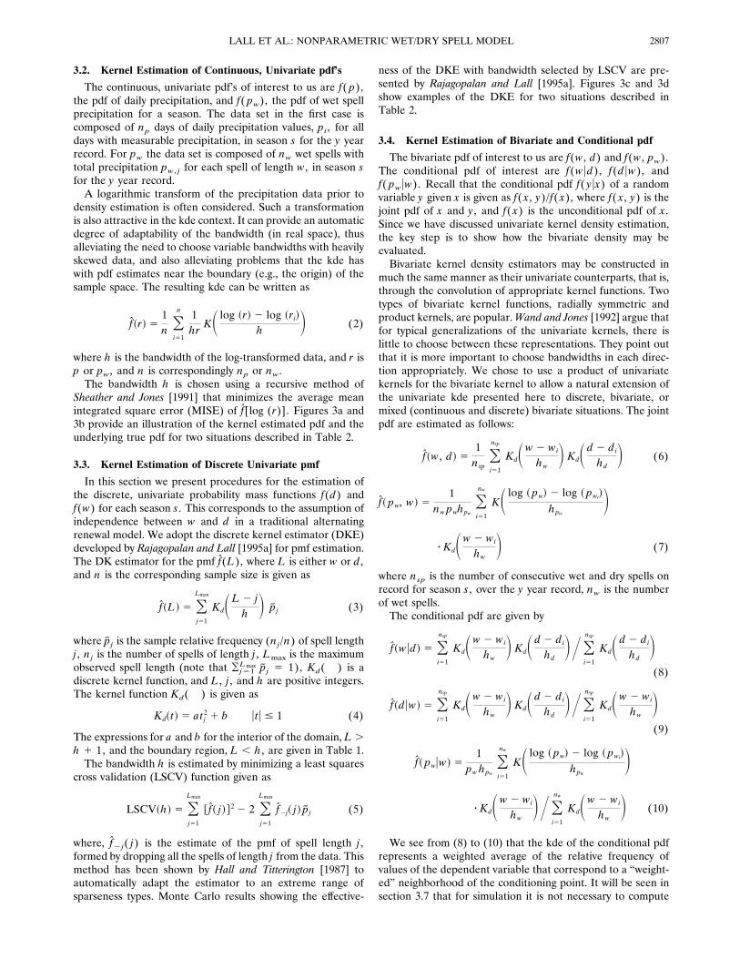
Sheather and Jones [1991] that minimizes the average meanintegrated square error (MISE) of f[log (r)]. Figures 3a and3b provide an illustration of the kernel estimated pdf and theunderlying true pdf for two situations described in Table 2.
3.3. Kernel Estimation of Discrete Univariate pmf
In this section we present procedures for the estimation ofthe discrete, univariate probability mass functions f(d) andf(w) for each season s. This corresponds to the assumption ofindependence between w and d in a traditional alternatingrenewal model. We adopt the discrete kernel estimator (DKE)developed by Rajagopalan and Lall [1995a] for pmf estimation.The DK estimator for the pmf f(L), where L is either w or d,and n is the corresponding sample size is given as
f~L! 5 Oj51
Lmax
KdSL 2 jh D p j (3)
where p j is the sample relative frequency (nj/n) of spell lengthj, nj is the number of spells of length j, Lmax is the maximumobserved spell length (note that • j51
Lmax p j 5 1), Kd( ) is adiscrete kernel function, and L, j, and h are positive integers.The kernel function Kd( ) is given as
Kd~t! 5 atj2 1 b ut u # 1 (4)
The expressions for a and b for the interior of the domain, L .h 1 1, and the boundary region, L , h, are given in Table 1.The bandwidth h is estimated by minimizing a least squares
cross validation (LSCV) function given as
LSCV~h! 5 Oj51
Lmax
@ f~ j!#2 2 2 Oj51
Lmax
f2j~ j! p j (5)
where, f2j( j) is the estimate of the pmf of spell length j ,formed by dropping all the spells of length j from the data. Thismethod has been shown by Hall and Titterington [1987] toautomatically adapt the estimator to an extreme range ofsparseness types. Monte Carlo results showing the effective-
ness of the DKE with bandwidth selected by LSCV are pre-sented by Rajagopalan and Lall [1995a]. Figures 3c and 3dshow examples of the DKE for two situations described inTable 2.
3.4. Kernel Estimation of Bivariate and Conditional pdf
The bivariate pdf of interest to us are f(w, d) and f(w, pw).The conditional pdf of interest are f(w ud), f(d uw), andf( pwuw). Recall that the conditional pdf f( y ux) of a randomvariable y given x is given as f( x , y)/f( x), where f( x, y) is thejoint pdf of x and y, and f( x) is the unconditional pdf of x.Since we have discussed univariate kernel density estimation,the key step is to show how the bivariate density may beevaluated.Bivariate kernel density estimators may be constructed in
much the same manner as their univariate counterparts, that is,through the convolution of appropriate kernel functions. Twotypes of bivariate kernel functions, radially symmetric andproduct kernels, are popular.Wand and Jones [1992] argue thatfor typical generalizations of the univariate kernels, there islittle to choose between these representations. They point outthat it is more important to choose bandwidths in each direc-tion appropriately. We chose to use a product of univariatekernels for the bivariate kernel to allow a natural extension ofthe univariate kde presented here to discrete, bivariate, ormixed (continuous and discrete) bivariate situations. The jointpdf are estimated as follows:
f~w, d! 51nsp
Oi51
nsp
KdSw 2 wihw
D KdS d 2 dihd
D (6)
f~ pw, w! 51
nw pwhpwOi51
nw
KS log ~ pw! 2 log ~ pwi!hpw
Dz KdSw 2 wi
hwD (7)
where nsp is the number of consecutive wet and dry spells onrecord for season s , over the y year record, nw is the numberof wet spells.The conditional pdf are given by
f~w ud! 5 Oi51
nsp
KdSw 2 wihw
D KdS d 2 dihd
DYOi51
nsp
KdS d 2 dihd
D(8)
f~d uw! 5 Oi51
nsp
KdSw 2 wihw
D KdS d 2 dihd
DYOi51
nsp
KdSw 2 wihw
D(9)
f~ pwuw! 51
pw hpwOi51
nw
KS log ~ pw! 2 log ~ pwi!hpw
Dz KdSw 2 wi
hwDYO
i51
nw
KdSw 2 wihw
D (10)
We see from (8) to (10) that the kde of the conditional pdfrepresents a weighted average of the relative frequency ofvalues of the dependent variable that correspond to a “weight-ed” neighborhood of the conditioning point. It will be seen insection 3.7 that for simulation it is not necessary to compute
2807LALL ET AL.: NONPARAMETRIC WET/DRY SPELL MODEL
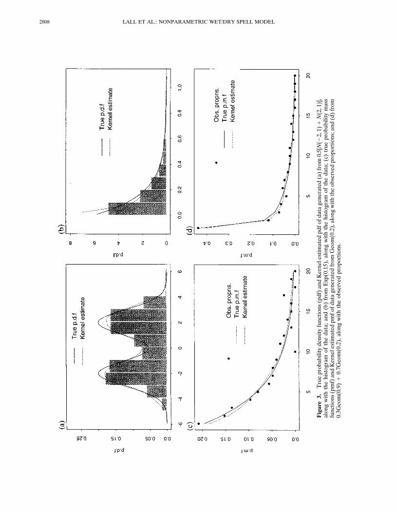
Figure3.
Trueprobabilitydensityfunctions(pdf)andKernelestimatedpdfofdatagenerated(a)from0.5[N(22,1)
1N(2,1)],
alongwiththehistogramofthedata;and(b)from
Exp(0.15),alongwiththehistogramofthedata;(c)trueprobabilitymass
functions(pmf)andKernelestimatedpmfofdatageneratedfromGeom(0.2),alongwiththeobservedproportions;and(d)from
0.3Geom(0.9)
10.7Geom(0.2),alongwiththeobservedproportions.
LALL ET AL.: NONPARAMETRIC WET/DRY SPELL MODEL2808

the joint and conditional pdf, estimation of the bandwidthsalone is sufficient.McLachlan [1992, pp. 306–308] discusses the simultaneous
selection of bandwidths in each coordinate versus the use ofthe optimal univariate bandwidths in each direction. It is notclear that the additional effort of simultaneous selection of thetwo bandwidths is justified. Consequently, we choose the band-widths hw, hd, and hpw by the methods described for theunivariate case.As an illustration, a sample of size 250 is generated from a
bivariate geometric distribution Geom (0.6, 0.2) were used totest this procedure. The surface of the observed proportions isplotted in Figure 4a, the true density surface is shown in Figure4b, the kernel estimated density surface is on Figure 4c and thedifference between the true and kernel estimates are plotted inFigure 4d. The bandwidth was 3 in the x direction and 6 in they direction. To illustrate the conditional kde, a slice is takenfrom the joint density in Figure 4c and presented in Figure 4e.In the precipitation data sets we have investigated thus far,
the correlation between w and d is generally weak, and theserial correlation between daily precipitation for fixed spelllength w is also weak. Thus, in most cases the univariate pdfsuffice. However, for the sake of completeness we describe anonparametric, kernel-based disaggregation strategy for disag-gregating a w day precipitation pw into w daily precipitationamounts pi.
3.5. Wet Spell Precipitation Disaggregation
We follow the approach of Aitchison and Lauder [1985] foranalyzing compositional data. A basic requirement for the dis-aggregation process is that • i51
w pi 5 pw. Consider the rescal-ing xi 5 pi/pw, so that 0 , xi , 1, and •xi 5 1. Recognizingthat the effective degrees of freedom are (w 2 1), we canwrite xw 5 1 2 • i51
w21 xi. Aitchison and Lauder [1985] nowapply the transform
yi 5 log ~ xi/xw! i 5 1, · · · , w 2 1 (11)
The multivariate pdf f(x), where x is a vector of length (w 21) representing the first (w 2 1) proportions, is then esti-mated using the kernel method with a logistic normal kerneland nw wet spells of length w as
f~x! 5 Oi51
nw 1nwL~x, x i, y, y i, h!
5 Oi51
nw [email protected]~y 2 y i!TSy21~y 2 y i!/h2#
nw~2p!~w21!/ 2h ~w21! det ~Sy!1/ 2 P j51w xji
(12)
where i is a spell index, y is a vector of length (w 2 1) asdefined in (12), xji represents the value of the jth componentof x for the ith spell, L(x, xi, y, yi, h) is the logistic normalkernel, h is a bandwidth, and Sy is the sample covariance
matrix of y, estimated using a robust method [see Huber, 1981].The bandwidth h is selected using maximum likelihood crossvalidation, that is, choosing h to maximize ) i51
nw f2i(xi), wheref2i(xi) is the estimate of f(x) at xi obtained by dropping the ithpoint. Aitchison and Lauder [1985] demonstrated that perfor-mance of this algorithm is comparable to parametric alterna-tives with sample sizes ranging from 23 to 95 for 2–10 compo-nents.The use of the sample covariance matrix Sy of y as the
covariance matrix for the kernel function for y leads to somedegree of preservation of the covariance structure of the com-ponents of y and hence of the disaggregated daily precipitationamounts pi. It also mitigates the effect of choosing xw, ratherthan say x1 as the normalizing variable in the transformation of(12).Using (13), one can evaluate the pdf of the first (w 2 1)
ratios xi of daily precipitation to wet spell precipitation. Astochastic realization of these ratios can then be generated.The last ratio xw is obtained by noting that all the ratios haveto sum to one. Daily precipitation values are then obtained bymultiplying xi by pw. This disaggregation procedure general-izes the logistic normal based disaggregation procedurethrough the use of the kernel method and admits multimodal-ity and heterogeneity in the pdf of daily rainfall in a wet spell.A problem with any wet/dry spell model is that as w increases,nw typically decreases. Consequently, this disaggregationscheme may not be practical for large w unless long records areavailable. Also, it fails to “borrow” information from spells oflength other than the one generated. However, that can be aproblem even for the usual parametric schemes.
3.6. Generation of Synthetic Sequences
Since our goal here is to generate random samples that aresimilar to the observed sequence, a “raw” bootstrap or resam-pling of the data with replacement from the observed datasequence could be considered as an alternative to samplingfrom the kde. Such a strategy would be equivalent to samplingfrom the empirical distribution function of the data. The kdecan be thought of as a smoothed (moving average) estimate ofthe derivative of the empirical distribution function. Samplingfrom the kde can lead to a reduced variance of the MonteCarlo design [Silverman, 1986, p. 145]. It also avoids the prob-lem with the bootstrap where a number of the historical valuesare repeated in a generated sample and provides an ability tofill in and extrapolate to a limited extent beyond the observedvalues.Synthetic precipitation sequences at a site are generated
continuously from season to season. A dry spell is first gener-ated using f(d). Following the strategy indicated in Figure 1, awet spell is generated using f(w) or f(w ud). Precipitation foreach of w days is then generated using f( p) or f( pwuw) fol-lowed by f( piupw). A dry spell is then generated using f(d) or
Table 2. Statistics of Known Distributions From Which a Sample of Size 250 was Taken to Test k.d.e. Methods
Figure Parent MethodSampleMean
Sample StandardDeviation
KernelBandwidth
3a {0.5N(22, 1) 1 0.5N(2, 1)} Epanechnikov kernel, SJ bandwidth 20.00 2.26 1.223b Exp (0.15) Log transform, Epanechnikov kernel, SJ bandwidth 0.16 0.18 0.943c Geom (0.2) Quadratic kernel, DK estimator, LSCV bandwidth 5.11 4.19 63d {0.3 Geom (0.9) 1 0.7 Geom (0.2)} Quadratic kernel, DK estimator, LSCV bandwidth 3.92 4.02 2
2809LALL ET AL.: NONPARAMETRIC WET/DRY SPELL MODEL
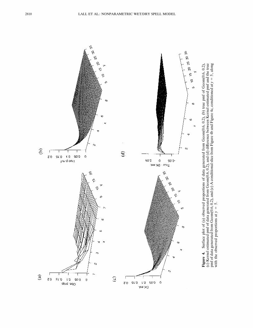
Figure4.
Surfaceplotof(a)observedproportionsofdatageneratedfrom
Geom(0.6,0.2),(b)truepmfofGeom(0.6,0.2),
(c)KernelestimatedpmfofdatageneratedfromGeom(0.6,0.2),and(d)differencebetweenKernelestimatedpmfandthetrue
pmfofdatageneratedfromGeom(0.6,0.2),and(e)AconditionalslicefromFigure4bandFigure4c,conditionedaty
55,along
withtheobservedproportionsaty
55.
LALL ET AL.: NONPARAMETRIC WET/DRY SPELL MODEL2810

f(d uw), and the process repeats. If a season boundary iscrossed, the pdf used switch to those for the new season.For the univariate continuous case ( f(r)), the random vari-
ate (r) of interest can be generated readily from the kerneldensity following a two-step procedure [Devroye, 1986, p. 765].Consider the original sample (ri, i 5 1, z z z , n) from whichthe kernel density (that depends on r, ri, and h) was con-structed using a Kernel function K( ). To generate a randomnumber r that follows the estimated distribution, first sample arandom integer j uniformly between 1 and n, that is, identifythe historical data point to perturb. Now generate a randomvariate U from the probability density corresponding to thekernel function K( ), (e.g., K(u) 5 3/4(1 2 u2) for theEpanechnikov kernel). The random variate r is then given by(rj 1 Uh). This reinforces the notion that the kernel densityestimator is formed as a convolution of local densities centeredat each observation and that the generated sequence will con-stitute a smoothed bootstrap of the data. Any of a number ofstandard procedures (e.g., based on order statistics or rejec-tion) for sampling from a density may be used to generate Ufrom the density K( ). Devroye [1986, p. 765] provides exam-ples for the Epanechnikov kernel. The discrete random vari-ables (w and d) are generated directly from the estimatedcumulative mass function.A similar strategy is possible for sampling from the condi-
tional pdf as well. Consider two continuous variables x and y.The conditional kernel density f( y ux) is given by
f~ y ux! 51hy
Oi51
n
KS y 2 yihy
D KS x 2 xihx
DYOi51
n
KS x 2 xihx
D
51hy
Oi51
n
wti KS y 2 yihy
D (13)
where wti 5 K( x 2 xi/hx)/• i51n K( x 2 xi/hx). Now note that
• i51n wti is equal to 1, and hence we can view the wti values asproviding the probability metric with which the ith point
should be selected. Define F as the set of probabilities wti.Sample an integer j [ [1, n] using F. Now sample a variate Ufrom the density corresponding to the kernel function for y .The variate of interest is then y 5 Uh 1 yj. The discretevariate case follows as before.
4. Model ApplicationThe model described was applied to daily rainfall data from
the Silver Lake station in Utah. Forty-four years of daily rain-fall data were available from 1948 to 1992. For this applicationwe have divided the year into four seasons: season 1 (January–March), season 2 (April–June), season 3 (July–September),season 4 (October–December). Alternate season definitions aswell as variable season lengths could be used. The demarcationof precipitation seasons can be based on the kernel smoothingprocedures described by Rajagopalan and Lall [1995b]. SilverLake is one of the higher-elevation stations in Utah, situated at408369N latitude, 1118359W longitude, and at an elevation of8740 feet (2664 m). Most of the precipitation comes in theform of winter snow and season 4 rainfall. We see from Table3 that season 4 (fall) has the highest mean wet day precipita-tion and maximum wet day precipitation, while season 1 (win-ter) has the highest percentage of yearly precipitation. Season1 (winter) has the highest average wet spell length and thelongest wet spell length. For the dry spells, season 3 (summer)has the highest average dry spell length and the longest dryspell length.The successive wet-dry spell and dry-wet spell length corre-
lations for the data from Silver Lake, Utah, were all near zerofor each season. We present a representative scatterplot of thelength of successive wet and dry spells for season 1 in Figure 5;the line in Figure 5 is the locally weighted regression (LOESS)smooth [Cleveland, 1979]. There is little evidence of even non-linear structure in the relationship. The correlations betweendaily precipitation amount on successive days within a spellwere also found to be near 0. Consequently, we simulated thewet and dry spells alternately using the unconditional densities
Figure 4. (continued)
2811LALL ET AL.: NONPARAMETRIC WET/DRY SPELL MODEL
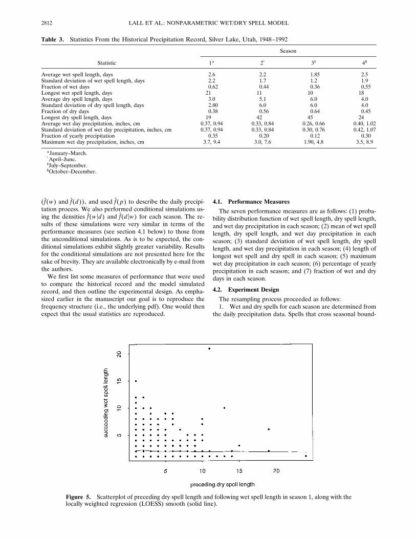
( f(w) and f(d)), and used f( p) to describe the daily precipi-tation process. We also performed conditional simulations us-ing the densities f(w ud) and f(d uw) for each season. The re-sults of these simulations were very similar in terms of theperformance measures (see section 4.1 below) to those fromthe unconditional simulations. As is to be expected, the con-ditional simulations exhibit slightly greater variability. Resultsfor the conditional simulations are not presented here for thesake of brevity. They are available electronically by e-mail fromthe authors.We first list some measures of performance that were used
to compare the historical record and the model simulatedrecord, and then outline the experimental design. As empha-sized earlier in the manuscript our goal is to reproduce thefrequency structure (i.e., the underlying pdf). One would thenexpect that the usual statistics are reproduced.
4.1. Performance Measures
The seven performance measures are as follows: (1) proba-bility distribution function of wet spell length, dry spell length,and wet day precipitation in each season; (2) mean of wet spelllength, dry spell length, and wet day precipitation in eachseason; (3) standard deviation of wet spell length, dry spelllength, and wet day precipitation in each season; (4) length oflongest wet spell and dry spell in each season; (5) maximumwet day precipitation in each season; (6) percentage of yearlyprecipitation in each season; and (7) fraction of wet and drydays in each season.
4.2. Experiment Design
The resampling process proceeded as follows:1. Wet and dry spells for each season are determined from
the daily precipitation data. Spells that cross seasonal bound-
Figure 5. Scatterplot of preceding dry spell length and following wet spell length in season 1, along with thelocally weighted regression (LOESS) smooth (solid line).
Table 3. Statistics From the Historical Precipitation Record, Silver Lake, Utah, 1948–1992
Statistic
Season
1* 2† 3‡ 4§
Average wet spell length, days 2.6 2.2 1.85 2.5Standard deviation of wet spell length, days 2.2 1.7 1.2 1.9Fraction of wet days 0.62 0.44 0.36 0.55Longest wet spell length, days 21 11 10 18Average dry spell length, days 3.0 5.1 6.0 4.0Standard deviation of dry spell length, days 2.80 6.0 6.0 4.0Fraction of dry days 0.38 0.56 0.64 0.45Longest dry spell length, days 19 42 45 24Average wet day precipitation, inches, cm 0.37, 0.94 0.33, 0.84 0.26, 0.66 0.40, 1.02Standard deviation of wet day precipitation, inches, cm 0.37, 0.94 0.33, 0.84 0.30, 0.76 0.42, 1.07Fraction of yearly precipitation 0.35 0.20 0.12 0.30Maximum wet day precipitation, inches, cm 3.7, 9.4 3.0, 7.6 1.90, 4.8 3.5, 8.9
*January–March.†April–June.‡July–September.§October–December.
LALL ET AL.: NONPARAMETRIC WET/DRY SPELL MODEL2812

Figure6.
PlotsofpdfofwetdayprecipitationforthefourseasonsatSilverLake,Utah,estimatedusingSheatherJonesLog
procedure,thefittedexponentialdistribution,fittedgammadistribution,andhistogramoftheobserveddata.
2813LALL ET AL.: NONPARAMETRIC WET/DRY SPELL MODEL

aries are truncated at the season boundary and included in theappropriate seasons. We recognize that this could have theeffect of introducing a small bias in the spell characteristics fora given season. Missing data are skipped, and the spell count isrestarted with the next event.2. Probability density/mass functions are fitted for the wet
day precipitation, wet spell lengths, and dry spell lengths foreach season using the kernel estimators recommended in sec-tion 3.3. Twenty-five synthetic records of 44 years each (i.e., the
historical record length) are simulated.4. The statistics of interest are computed for each simu-
lated record and for each season and compared to statistics ofthe historical record using boxplots.
5. ResultsIn this section we present comparative results (using the
performance measures listed in section 4.1) of the NSS modelfor the Silver Lake data. The statistics (pdfs) of the simulatedrecords are compared with those for the historical record usingboxplots. A box in the boxplots (e.g., Figure 7) indicates theinterquartile range of the statistic computed from 25 simula-tions, the line in the middle of the box indicates the mediansimulated value. The solid lines correspond to the statistic ofthe historical record. The boxplots show the range of variationin the statistics from the simulations and also show the capa-bility of the simulations to reproduce historical statistics. Theplots of the pdf are truncated to show a common range acrossseasons and to highlight differences near the origin (mode).
5.1. Wet Day Precipitation
Figure 6 shows that the fitted kernel densities for wet dayprecipitation amount are similar to the histogram of the re-corded data in all four seasons. They differ from the fittedexponential and gamma distribution, particularly in seasons 3(summer) and 4 (fall). The kernel estimated pdf’s of the sim-ulated data reproduce the pdf of the historical data quite well,as can be seen in Figure 7. The other statistics are reproducedwell by the model, as can be seen from the boxplots in Figure 8.
5.2. Wet Spell Length
Figure 9 shows that the pmf’s of wet spell length estimatedby DKE and the fitted geometric distribution are very close(except perhaps for season 1 (winter)). In this case one couldargue for using the geometric distribution rather than DKE.However, the “loss” in using DKE is small and for uniformapplication across sites, DKE may still be a better choice. Thepmf of wet spell length from the simulations reproduce thehistorical pdf very well in all the seasons as can be noted fromFigure 10, suggesting that the model is performing well inreproducing the underlying frequency structure. Figure 11shows that the mean, standard deviation, fraction of wet days,and longest wet spell length are all well reproduced by themodel.
5.3. Dry Spell Length
Figure 12 shows that the dry spell length pmf estimated byDKE and the fitted geometric distribution are generally similarwith the most difference in season 3 (summer), which we notedas being the most “active” with regard to dry spell lengthextremes. Observationally, we know that there are dry sum-mers with little rainfall activity and other summers with inter-
mittent, stagnating precipitation systems in this area. Thus wewould expect a mixture of mechanisms generating dry spells toshow up in this season.The pmf of wet spell length from the simulations reproduce
the historical pdf very well in all the seasons as can be notedfrom Figure 13, suggesting that the model is performing well inreproducing the underlying frequency structure. Figure 14shows that the statistics of the dry spell length are also wellreproduced.The reader may be tempted to suggest formal tests to check
for a mixture of the geometric distributions in this case as analternative to the kernel density estimate. While this may be afruitful activity (we did consider it), it gets harder to performand/or justify as we consider arbitrary, finite component mix-tures. An advantage of the DKE employed here is that itreadily admits such mixtures without requiring that they behypothesized or formally identified. We feel that this providesa more direct and parsimonious representation of this sort ofstructure if present in the data.
6. Summary and ConclusionsA nonparametric methodology for simulating daily precipi-
tation is presented in this paper. The traditional wet/dry spellmodel is extended to (1) consider heterogeneity in the pdf ofprecipitation or wet/dry spell length and (2) consider depen-dence between wet/dry spell length, and between wet spelllength and spell precipitation. The latter may or may not beimportant for rainfall data. All functions of interest are esti-mated nonparametrically. The primary intended use of themodel is as a simulator that is faithful to the historical datasequence. The pdf’s evaluated are also likely to be of use forjustifying the use of other formal, parametric models of theunderlying process.While a rather flexible framework is provided by the model
proposed, it is not without a price. Sample sizes needed forestimating the pdf of interest are likely to be larger than forparametric estimation. However, the nonparametric specifica-tion of the pdf leads to robustness with respect to the mis-specification of the parametric model which may be valuable ifthe use of a particular model is to be legislated across a varietyof sites and regions with different attributes. Only a crudetreatment for seasonal nonstationarity is offered. This is some-thing we expect to address in the future.A number of issues of interest to stochastic precipitation
modelers were not discussed here. The foremost is the behav-ior of the proposed model at different timescales. We view ourdevelopments as “operational” and relevant to the timescale ofthe data, which was daily. Spell definitions are tenuous at bestat finer timescales and sample sizes drop rapidly as longertimescales (e.g., monthly or annual) are considered. Thus,while the scaling issue is of theoretical and practical interest, itis difficult to formally assess how such a model may fit in. It isan issue we expect to explore in due course. A second issue isthe need to incorporate climatic or precipitation “types” [e.g.,Bogardi et al., 1993; Wilson and Lattenmaier, 1993] into thedaily precipitation model. We feel that implicit considerationof some of these factors is provided by our model by admittingan arbitrary mixture of generating mechanisms. Transitionsbetween generating mechanisms are not explicitly modeled.However, their relative frequencies ought to be reproduced.Given limited data sets and the potentially large number ofgenerating mechanisms this may be all that is reliably feasible
LALL ET AL.: NONPARAMETRIC WET/DRY SPELL MODEL2814
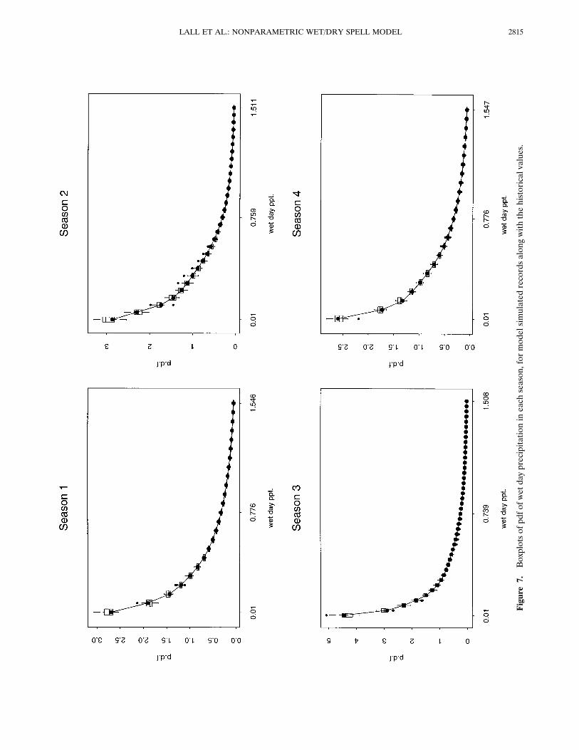
Figure7.
Boxplotsofpdfofwetdayprecipitationineachseason,formodelsimulatedrecordsalongwiththehistoricalvalues.
2815LALL ET AL.: NONPARAMETRIC WET/DRY SPELL MODEL

Figure8.
Boxplotsofmean,standarddeviation,fractionofyearlyprecipitation,andmaximum
precipitationofwetday
precipitationineachseasonformodelsimulationsalongwiththehistoricalvalues.
LALL ET AL.: NONPARAMETRIC WET/DRY SPELL MODEL2816

Figure9.
PlotsofpmfofwetspelllengthforthefourseasonsatSilverLake,Utah,estimatedusingdiscretekernelestimator
(DKE).Alongwiththefittedgeometricdistributionandobservedproportions.
2817LALL ET AL.: NONPARAMETRIC WET/DRY SPELL MODEL
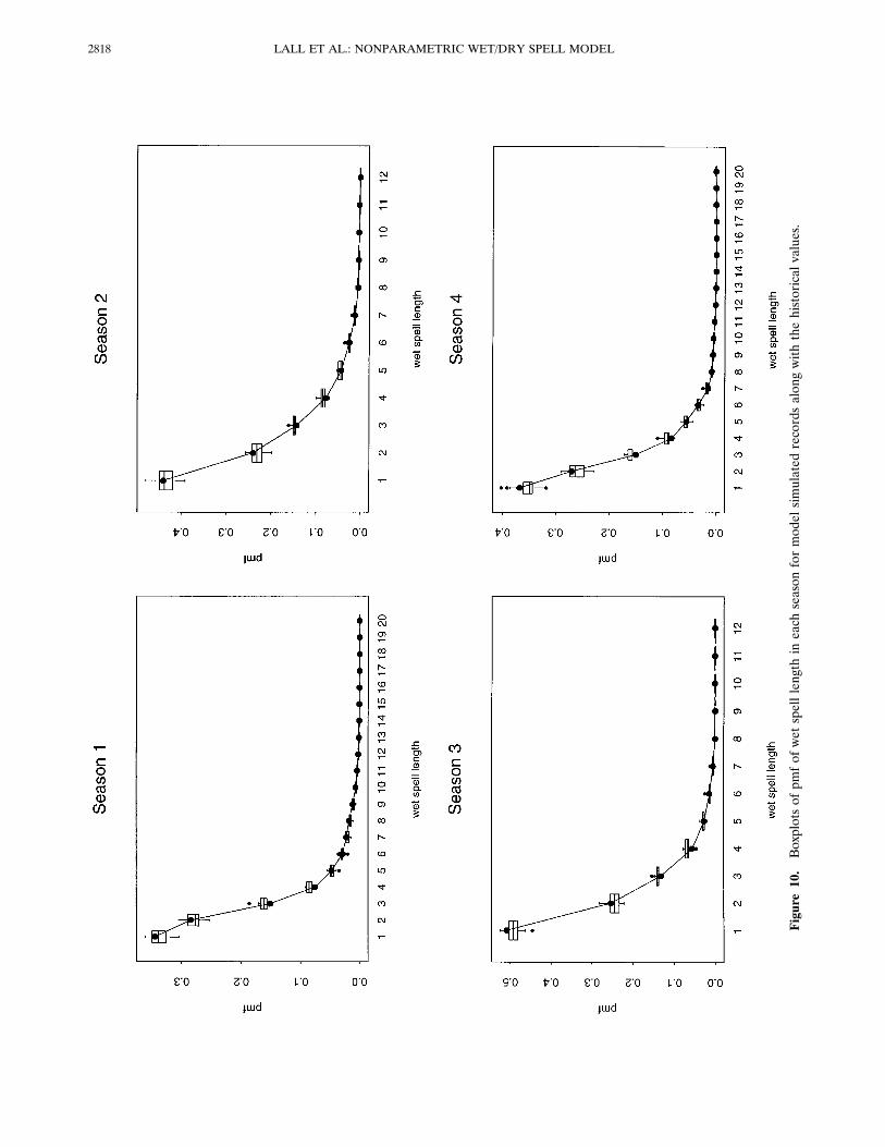
Figure10.Boxplotsofpmfofwetspelllengthineachseasonformodelsimulatedrecordsalongwiththehistoricalvalues.
LALL ET AL.: NONPARAMETRIC WET/DRY SPELL MODEL2818

Figure11.Boxplotsofmean,standarddeviation,fractionofwetdays,andlongestwetspelllengthineachseasonformodel
simulationsmadealongwiththehistoricalvalues.
2819LALL ET AL.: NONPARAMETRIC WET/DRY SPELL MODEL
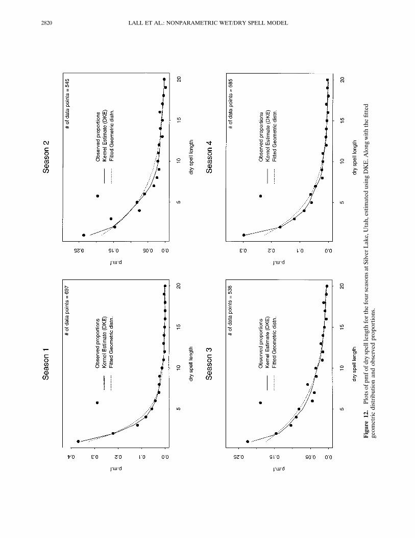
Figure12.PlotsofpmfofdryspelllengthforthefourseasonsatSilverLake,Utah,estimatedusingDKE.Alongwiththefitted
geometricdistributionandobservedproportions.
LALL ET AL.: NONPARAMETRIC WET/DRY SPELL MODEL2820
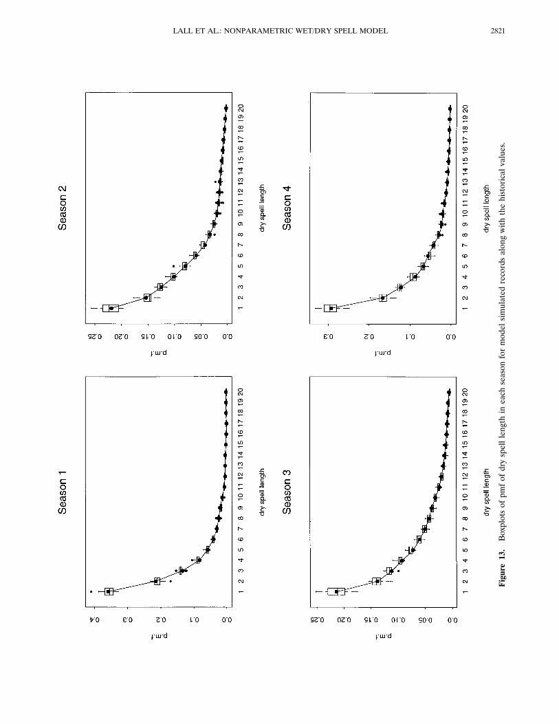
Figure13.Boxplotsofpmfofdryspelllengthineachseasonformodelsimulatedrecordsalongwiththehistoricalvalues.
2821LALL ET AL.: NONPARAMETRIC WET/DRY SPELL MODEL
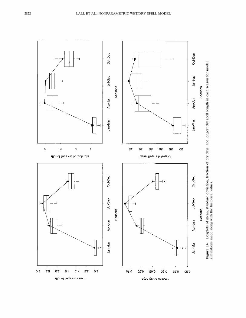
Figure14.Boxplotsofmean,standarddeviation,fractionofdrydays,andlongestdryspelllengthineachseasonformodel
simulationsmadealongwiththehistoricalvalues.
LALL ET AL.: NONPARAMETRIC WET/DRY SPELL MODEL2822

in a number of cases. Finally, there is the question of region-alization and/or portability of the method. The nonparametricapproach clearly enjoys broader applicability than its paramet-ric competitors. On the other hand, it may be less amenable todirect regionalization as is sometimes done in terms of theparameters of a parametric distribution. It is meaningless totalk of a regional bandwidth. It may be more fruitful to developa space-time nonparametric precipitation model with a non-homogeneous point process structure that is inferred from thedata.
Acknowledgments. Partial support of this work by the U.S. ForestService under contract INT-92660-RJVA, Amend 1 is acknowledged.We are grateful for discussions with D. S. Bowles, the Principal Inves-tigator for this project. Finally, we thank M. C. Jones, H. G. Muller,S. J. Sheather, J. Simonoff, and J. Dong for stimulating discussions onkernel density estimation, review, and provision of relevant manu-scripts and codes.
ReferencesAitchison, J., and I. J. Lauder, Kernel density estimation for compo-sitional data, Appl. Stat., 34(2), 129–137, 1985.
Bogardi, I., I. Matyasovszky, A. Bardossy, and L. Duckstein, Applica-tion of space-time stochastic model for daily precipitation usingatmospheric circulation patterns, J. Geophys. Res., 98, 16,653–16,667,1993.
Cayan, D., and L. Riddle, Atmospheric circulation and precipitation inthe Sierra Nevada, Managing water resources during global change,paper presented at Conference of American Water Resources As-sociation, Tucson, Ariz., 1992.
Chang, T. J., M. L. Kavvas, and J. W. Delleur, Daily precipitationmodeling by discrete autoregressive moving average processes, Wa-ter Resour. Res., 20, 565–580, 1984.
Chin, E. H., Modeling daily precipitation occurrence process withMarkov Chain, Water Resour. Res., 13, 949–956, 1977.
Cleveland, W. S., Robust locally weighted regression and smoothingscatter plots, J. Am. Stat. Assoc., 74, 829–836.
Devroye, L., Non-Uniform Random Variate Generation, Springer-Verlag, New York, 1986.
Feyerherm, A. M., and L. D. Bark, Statistical methods for persistentprecipitation patterns, J. Appl. Meteorol., 4, 320–328, 1965.
Feyerherm, A. M., and L. D. Bark, Goodness of fit of a markov chainmodel for sequences of wet and dry days, J. Appl. Meteorol., 6,770–773, 1967.
Foufoula-Georgiou, E., and D. P. Lettenmaier, A markov renewalmodel for rainfall occurrences, Water Resour. Res., 23, 875–884,1987.
Foufoula-Georgiou, E., and K. P. Georgakakos, Recent advances inspace-time precipitation modeling and forecasting, Recent Advancesin the Modelling of Hydrologic Systems, NATO ASI Ser. 1988.
Georgakakos, K. P., and M. L. Kavvas, Precipitation analysis, model-ing, and prediction in hydrology, Rev. Geophys., 25(2), 163–178,1987.
Guzman, A. G., and C. W. Torrez, Daily rainfall probabilities: Condi-tional upon prior occurrence and amount of rain, J. Clim. Appl.Meteorol., 24(10), 1009–1014, 1985.
Haan, C. T., D. M. Allen, and J. O. Street, A markov chain model ofdaily rainfall, Water Resour. Res., 12, 443–449, 1976.
Hall, P., and D. M. Titterington, On smoothing sparse multinomialdata, Aust. J. Stat., 29(1), 19–37, 1987.
Hardle, W., Smoothing Techniques With Implementation in S, Springer-Verlag, New York, 1991.
Hopkins, J. W., and P. Robillard, Some statistics of daily rainfalloccurrence for the canadian prairie provinces, J. Appl. Meteorol., 3,600–602, 1964.
Huber, P. J., Robust Statistics, New York, John Wiley, 1981.Katz, R. W., and M. B. Parlange, Effects of an index of atmosphericcirculation on stochastic properties of precipitation, Water Resour.Res., 29, 2335–2344, 1993.
Lall, U., Recent advances in nonparametric function estimation, U.S.Natl. Rep. Int. Union Geod. Geophys. 1991–1994, Rev. Geophys., 33,1093–1102, 1995.
McLachlan, G. J., Discriminant Analysis and Statistical Pattern Recog-nition, John Wiley, New York, 1992.
Rajagopalan, B., and U. Lall, A kernel estimator for discrete distribu-tions, J. Nonparametric Stat., 4, 409–426, 1995a.
Rajagopalan, B., and U. Lall, Seasonality of precipitation along ameridian in the western U.S., Geophys. Res. Lett., 22(9), 1081–1084,1995.
Roldan, J., and D. A. Woolhiser, Stochastic daily precipitation models,1, A comparison of occurrence processes, Water Resour. Res., 18,1451–1459, 1982.
Scott, D. W., Multivariate Density Estimation: Theory, Practice andVisualization, John Wiley, New York, 1992.
Sheather, S. J., and M. C. Jones, A reliable data-based bandwidthselection method for kernel density estimation, J. R. Stat. Soc., Ser.B, 53, 683–690, 1991.
Silverman, B. W., Density Estimation for Statistics and Data Analysis,Chapman and Hall, New York, 1986.
Srikanthan, R., and T. A. McMahon, Stochastic simulation of dailyrainfall for Australian stations. Trans. ASAE, 754–766, 1983.
Vogel, R. M., and D. E. McMartin, Probability plot goodness-of-fit andskewness estimation procedures for the Pearson type 3 distribution,Water Resour. Res., 27, 3149–3158, 1991.
Wand, J. S., and M. C. Jones, Comparison of smoothing parameter-izations in bivariate kernel density estimation, J. Am. Stat. Assoc.,88(422), 520–528, 1992.
Waymire, E., and V. K. Gupta, The mathematical structure of rainfallrepresentations, 1, A review of the stochastic rainfall models, WaterResour. Res., 17(5), 1261–1272, 1981a.
Waymire, E., and V. K. Gupta, The mathematical structure of rainfallrepresentations, 2, A review of the theory of point processes, WaterResour. Res., 17(5), 1273–1285, 1981b.
Waymire, E., and V. K. Gupta, The mathematical structure of rainfallrepresentations, 3, Some applications of the point process theory torainfall processes, Water Resour. Res., 17(5), 1287–1294, 1981c.
Webb, R. H., and J. L. Bettencourt, Climatic variability and floodfrequency of the Santa Cruz river, Pima County, Arizona, U.S. Geol.Surv. Water Supply Pap., 2379, 1992.
Wilson, L. L., and D. P. Lettenmaier, A hierarchical stochastic-modelof large-scale atmospheric circulation patterns and multiple stationdaily precipitation, J. Geophys. Res., 97, 2791–2809, 1993.
Woolhiser, D. A., C. L. Hanson, and C. W. Richardson, Microcom-puter program for daily weather simulation, Rep. 75, 49 pp., Agric.Research Serv., U.S. Dep. of Agric., Washington, D. C., 1988.
U. Lall and D. G. Tarboton, Department of Civil and Environmen-tal Engineering, Utah State University, Logan, UT 84322-8200.(e-mail: [email protected];B. Rajagopalan, Lamont-Doherty Earth Observatory of Columbia
University, P.O. Box 1000, Route 9W, Palisades, NY 10964-8000.(e-mail: [email protected])
(Received February 13, 1995; revised February 15, 1996;accepted February 16, 1996.)
2823LALL ET AL.: NONPARAMETRIC WET/DRY SPELL MODEL