A ‘nondecimated’ lifting transform

Marina I. Knight and Guy P. NasonDepartment of Mathematics, University of Bristol, UK

25th January 2008

Abstract

Classical nondecimated wavelet transforms are attractive for many applications. When the data comesfrom complex or irregular designs, the use of second generation wavelets in nonparametric regressionhas proved superior to that of classical wavelets. However, the construction of a nondecimated secondgeneration wavelet transform is not obvious. In this paper we propose a new ‘nondecimated’ liftingtransform, based on the lifting algorithm which removes one coefficient at a time, and explore itsbehaviour. Our approach also allows for embedding adaptivity in the transform, i.e. wavelet functionscan be constructed such that their smoothness adjusts to the local properties of the signal. We addressthe problem of nonparametric regression and propose an (averaged) estimator obtained by using ournondecimated lifting technique teamed with empirical Bayes shrinkage. Simulations show that ourproposed method has higher performance than competing techniques able to work on irregular data.Our construction also opens avenues for generating a ‘best’ representation, which we shall explore.

Keywords: wavelets, lifting, nondecimation, nonparametric regression, basis averaging.

1 Introduction

The nondecimated wavelet transform (NDWT) is well established in the current literature, see forinstance Holschneider et al. (1989), who use the term ‘algorithm trous’, Nason and Silverman(1995), who refer to it as the ‘stationary’ wavelet transform, Percival (1995) who proposes it under thename of maximal overlap discrete wavelet transform and Pesquet et al. (1996) . Coifman and Donoho(1995) propose ‘cycle spinning’, a technique for nonparametric regression equivalent to using waveletshrinkage on the nondecimated wavelet coefficients. These papers point out the appeal of producing awavelet transform which does not use decimation at each step, and Coifman and Donoho (1995) showthe superiority of cycle spinning over typical wavelet shrinkage techniques.

In this paper we assume a basic knowledge of wavelet transforms (for detailed descriptions thereader can refer to Daubechies (1992), Vidakovic (1999) or, for a brief review, to Abramovich et al.(2000)), and only briefly present the main points of the classical NDWT.

The scope of our paper is to propose a new ‘nondecimated’ lifting transform (NLT), capableof working on irregular data sets of any length. The basic frame on which we build our transformconsists of the lifting scheme, introduced by Sweldens (1996). The lifting algorithm still aims toprovide a wavelet-like representation of a signal using few (wavelet) coefficients, and the wavelet

Corresponding author: Marina.Knight@bristol.ac.uk

1

functions obtained through the lifting construction are referred to in the current literature as ‘secondgeneration’. In our work we shall use the version of the lifting scheme that ‘removes one coefficientat a time’, as proposed by Jansen et al. (2001, 2004). This will also allow us to use adaptivity in ournondecimated lifting transform, see Nunes et al. (2006) for details on an adaptive lifting scheme.

We embed our proposed transform into the wavelet shrinkage approach and apply it to nonpara-metric regression problems. We demonstrate by simulation the superiority of our method over previ-ous successful denoising techniques able to work on irregular data.

The paper is structured as follows. Section 2 briefly reviews the nondecimated wavelet transformand its application in nonparametric regression, as well as the lifting paradigm with removal of onecoefficient at a time. Section 3 proposes a modified lifting algorithm and the new NLT we constructbased on it. Section 4 deals with the application of the proposed NLT in nonparametric regression,proposes an (averaged) estimator and investigates its performance. Various characteristics of the al-gorithm are discussed, and comparisons with previous methods are performed. Furthermore, we willinvestigate ways of generating a ‘best’ representation, in a sense to be defined.

2 Wavelet methods and nonparametric regression

2.1 Nondecimated wavelet transform (NDWT)

In a nutshell, the NDWT ‘fills in the gaps’ caused by the decimation in the discrete wavelet transform(DWT). While the DWT produces wavelet coefficients for each scale , at dyadic locations of theform , where , the NDWT produces a wavelet coefficient at each integer locationwithin each scale.

The NDWT is an over-determined transform of the data, and its inverse is not unique. For detailson the relationships between the wavelet coefficients obtained by the NDWT and those obtained bythe DWT, and for possible approaches for inverting the NDWT, the reader can consult Nason andSilverman (1995). Notably, Coifman and Donoho (1995) show that thresholding the nondecimatedwavelet coefficients of a noisy signal results in a signal with smaller risk and significantly less visualartifacts than when applying the usual wavelet shrinkage.

2.2 Lifting scheme

In the mid 90’s, the lifting algorithm was introduced (Sweldens, 1996) partly in order to facilitate awavelet construction for non-standard data, including irregular data on a grid.

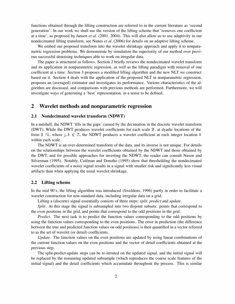
Lifting a (discrete) signal essentially consists of three steps: split, predict and update.Split. At this stage the signal is subsampled into two disjoint subsets: points that correspond to

the even positions in the grid, and points that correspond to the odd positions in the grid.Predict. The next task is to predict the function values corresponding to the odd positions by

using the function values corresponding to the even positions. The error in prediction (the differencebetween the true and predicted function values on odd positions) is then quantified in a vector referredto as the set of wavelet (or detail) coefficients.

Update. The function values on the even positions are updated by using linear combinations ofthe current function values on the even positions and the vector of detail coefficients obtained at theprevious step.

The split-predict-update steps can be re-iterated on the updated signal, and the initial signal willbe replaced by the remaining updated subsample (which reproduces the coarse scale features of theinitial signal) and the detail coefficients which accumulate throughout the process. This is similar

2

Split Predict Update

Figure 1: Schematic representation of the lifting scheme, where denotes the function valuescorresponding to the odd/even positions in the grid, and is the vector of details produced in theprediction stage. The process is then re-iterated on .

to the DWT which replaces the initial signal by a set of scaling and wavelet coefficients. A graphicrepresentation (Figure 1) shows this process.

The procedure is easily inverted by undoing the update stage, the prediction stage and then merg-ing the subsamples.

Variations on the split-predict-update stages exist in the literature. We presented above the liftingscheme using a data split into odd and even indices (Sweldens, 1996, 1998), while Jansen et al. (2001,2004) propose generating just one wavelet coefficient at each step. Claypoole et al. (1998, 2003) andPiella and Heijmans (2002) use a split-update-predict algorithm through which they adaptively buildwavelets. Nunes et al. (2006) use the flexibility of the lifting scheme that removes one coefficient at atime in order to build adaptive prediction steps and embed them into the lifting algorithm.

For the purposes of this paper we shall concentrate on the approach of Jansen et al. (2001, 2004),as we shall exploit some of its features. Hence, we shall now review some details on the liftingalgorithm that removes one coefficient at a time.

2.3 Lifting one coefficient at a time (LOCAAT)

Let us assume we have a function sampled at a set of possibly irregular locations, .We simply represent the observed function as . We start with (initial) scaling coef-ficients given by , and aim to transform them by means of lifting into a set of say,scaling and wavelet coefficients, where is the desired primary resolution level.

The split step of the lifting algorithm consists in choosing a point to be removed. The odd/evensplit poses problems in higher dimensions, and Jansen et al. (2001, 2004) introduce the concept oflifting just one coefficient at each step, which has greater flexibility and can be used in any dimen-sion. In essence, Jansen et al. (2001, 2004) propose to remove points in an order dictated by the -configuration: those points corresponding to denser areas are removed first, and further steps generatedetail in progressively coarser areas. Each location is associated with an interval which it intuitively‘spans’: the shorter the interval, the denser is the area it is coming from.

Once a point has been selected for removal, denote it by , we identify its set of neigh-bours, , and the next step (predict) is to predict by using regression over the neighbouringlocations . The prediction error, denote it by , will be the detail coefficient corresponding to that

3

location, and is given by(1)

where are the weights resulting from the regression procedure over , or in the one neigh-bour case,

(2)

In the update step, only the -values of the neighbouring points are updated by using a linearcombination with the detail coefficient,

(3)

where the weights are obtained from the requirement that the application of the algorithmshould keep constant the mean value of the signal.

At this stage, the length of the intervals associated to the neighbouring points also get updated, toaccount for the decreasing number of scaling points that remain to ‘span’ the same interval.

The procedure is then repeated on the updated signal, and with each repetition a new waveletcoefficient is added. Hence after say removals, we have scaling coefficients andwavelet coefficients.

In the second generation wavelet approach, although the signal is still represented on a fine–coarserange, the scaling and wavelet functions at the same level (stage) are not scaled versions of the samefunction as in the classical case.

The notion of scale itself is not obvious anymore, and Jansen et al. (2004) propose an artificial splitinto levels such that the length of the interval associated to each location at the stage of its removal,uniquely classifies it into an artificial level. The irregularity in locations is therefore reflected in thescale, which becomes a continuous quantity.

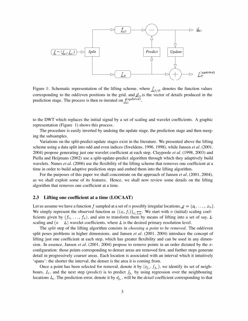
For further details about the LOCAAT construction and its interpretation, the reader is directedto Jansen et al. (2001, 2004), while for details on an adaptive lifting scheme built on LOCAAT, thereader can consult Nunes et al. (2006).Example: application of LOCAAT to a signal.Let us consider the simulated signal in Figure 2, sampled at 256 regularly spaced time points, out

of which 56 observations are deemed missing. The signal is a realization of a process whose secondorder structure varies slowly with time (Nason et al., 2000) and is, due to the missing data, observedon an irregular time grid of length .

In order to transform this signal into a set of detail and scaling coefficients, we shall apply LO-CAAT with a prediction step consisting of linear regression with an intercept over symmetrical neigh-bourhoods of size 2 (i.e. take the left and right neighbour of each point).

A few points are associated to intervals of smallest length, and the first point chosen for removalis time 1. Being a boundary point, this time point only has a right neighbour, time 2.

In the prediction step, the signal value of time 2 will be used for predicting the signal value attime 1, and the corresponding detail calculated as the difference between these two values, accordingto formula (2). The signal value for time 2 will then be updated (see equation (3)), and so will be itscorresponding interval length, to account for the larger area which time 2 now spans.

The procedure is then continued, with time 5 selected for removal, whose neighbourhood consistsof time points 4 and 6. The signal value of time 5 is therefore predicted to be the value given by theregression line fitted to the data corresponding to time points 4 and 6, and the detail is computed asthe difference between the observed and fitted signal values (as in equation (1)). In the update stage,

4

Figure 2: Simulated process of length featuring missing observations. Triangles indicate locationsof missing time points.

the signal values of times 4 and 6 get updated, and their interval lengths also get updated to accountfor the larger areas they now span.

The algorithm is repeated, time point 9 is next removed and a detail produced, and so on, untilonly two time points are left. These are times 43 and 126, and their signal values are referred to asscaling coefficients. The scaling coefficients no longer equal the initial values, as time points 43 and126 appeared in the course of the algorithm as neighbours for points that have been removed, andhave therefore had their signal values updated.

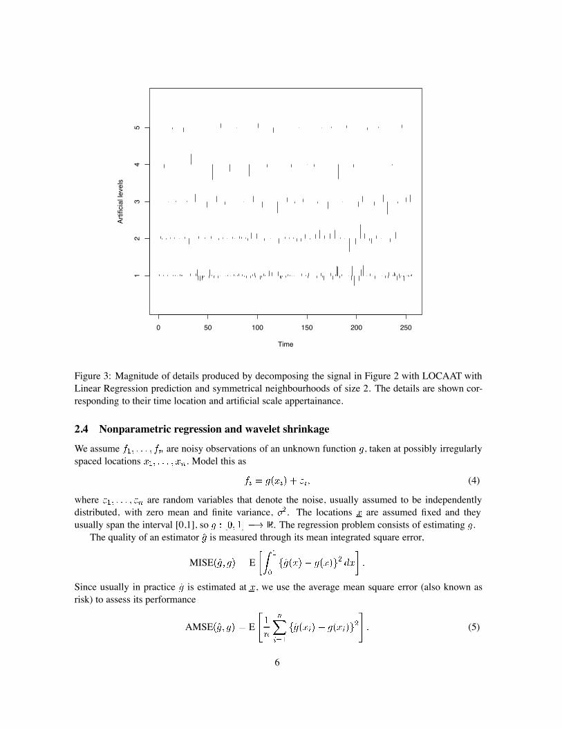
Figure 3 shows all (198) details that have been obtained by transforming the initial signal into aset of scaling and detail coefficients.

The lifting algorithm generates 5 artificial scale levels in which the details are arranged, followingan artificial dyadic split: the finest level (first artificial level) contains half of the wavelet coefficients,the next coarser level (second artificial level) a quarter, and so on. For easier reference to the classicalwavelet transform, we chose to display the wavelet coefficients in Figure 3 over both time and artificialscale.

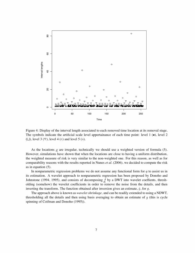
Figure 4 gives a better representation of how points get associated to artificial scales: the loca-tions associated to narrower intervals correspond to finer detail areas, while those associated to largerintervals generate information at coarser scale.

5

0 50 100 150 200 250

Time

Artif

icia

l lev

els

12

34

5

Figure 3: Magnitude of details produced by decomposing the signal in Figure 2 with LOCAAT withLinear Regression prediction and symmetrical neighbourhoods of size 2. The details are shown cor-responding to their time location and artificial scale appertainance.

2.4 Nonparametric regression and wavelet shrinkage

We assume are noisy observations of an unknown function , taken at possibly irregularlyspaced locations . Model this as

(4)

where are random variables that denote the noise, usually assumed to be independentlydistributed, with zero mean and finite variance, . The locations are assumed fixed and theyusually span the interval [0,1], so . The regression problem consists of estimating .

The quality of an estimator is measured through its mean integrated square error,

MISE E

Since usually in practice is estimated at , we use the average mean square error (also known asrisk) to assess its performance

AMSE E (5)

6

0 50 100 150 200 250

020

4060

80

Time

Inte

rval

leng

ths

Figure 4: Display of the interval length associated to each removed time location at its removal stage.The symbols indicate the artificial scale level appertainance of each time point: level 1 ( ), level 2( ), level 3 ( ), level 4 ( ) and level 5 ( ).

As the locations are irregular, technically we should use a weighted version of formula (5).However, simulations have shown that when the locations are close to having a uniform distribution,the weighted measure of risk is very similar to the non-weighted one. For this reason, as well as forcomparability reasons with the results reported in Nunes et al. (2006), we decided to compute the riskas in equation (5).

In nonparametric regression problems we do not assume any functional form for to assist us inits estimation. A wavelet approach to nonparametric regression has been proposed by Donoho andJohnstone (1994, 1995), and consists of decomposing by a DWT into wavelet coeffients, thresh-olding (somehow) the wavelet coefficients in order to remove the noise from the details, and theninverting the transform. The function obtained after inversion gives an estimate, , for .

The approach above is known as wavelet shrinkage, and can be readily extended to using a NDWT,thresholding all the details and then using basis averaging to obtain an estimate of (this is cyclespinning of Coifman and Donoho (1995)).

7

3 A ‘nondecimated’ lifting transform (NLT)

3.1 Introduction

Clearly, the nondecimated wavelet transform has properties which make it a better choice than theDWT for certain problems (Percival and Walden, 2000). However, like any other classical wavelettechnique, the fast NDWT has its limitations: it is designed to work on regularly spaced sequences oflength of the form , for some . It is often the case for real data to have missing observationson a regular grid, or for the function not to have been observed at regularly spaced intervals in the firstplace. It has already been shown (Claypoole et al. (1998), Trappe and Liu (2000), Nunes et al. (2006))that second generation wavelet methods can perform better than classical ones in such situations.

Claypoole et al. (1998) propose a redundant version of the lifting transform which splits the dataat each step into odds and evens. They evaluate the performance of the redundant lifting transformcombined with a hard threshold for nonparametric regression and the results are encouraging.

Lee et al. (2000) propose what they refer to as an ‘undecimated wavelet transform’ based on thelifting scheme. Their construction skips the split step, upsamples the lifting operators at each stage,in an algorithm which mimicks the classical NDWT. The only assessment is provided by an exampleof successful denoising of a Blocks (Donoho and Johnstone, 1994) signal.

The following work was motivated by the need to have information in the wavelet domain at allscales and locations, when the data is collected on an irregular grid. Here scale is to be understood inthe second generation sense, as explained in section 3.3.

Next, we shall propose a new wavelet transform that brings together some desirable properties:

It works on irregularly spaced data of any length.

It produces wavelet coefficients at each location, , and scale.

As already mentioned, our construction is based on LOCAAT (Jansen et al., 2001, 2004). Recallthat in the initial version of the LOCAAT, at each step the choice of point to be removed is based on thecurrent configuration of data points: start with scaling coefficients, and at each stage remove a pointfrom the most densely sampled region. The removal of such points will only cause a small informationloss in the signal. After generating each wavelet coefficient, the configuration is updated to accountfor the fewer points associated to scaling coefficients. This strategy, while proving successful (Jansenet al. (2004), Nunes et al. (2006)), is, of course, highly dependent on the removal order.

We challenge this construction by asking the question: is the LOCAAT sequence selection algo-rithm the ‘best’ order in which to remove points? Of course the sense of ‘best’ changes its meaningaccording to the problem we are trying to answer. We might have a compression problem, in whichcase sparsity of the wavelet coefficients is important, or a nonparametric regression problem, in whichcase achieving a signal estimate with small AMSE is of primary interest.

Our innovation consists in allowing full flexibility in the order of point removal, as we shalldescribe next.

3.2 Proposed NLT

We first propose a modified version of the Jansen et al. (2004) lifting algorithm which accommodatesany removal order of generating the wavelet coefficients.

Let us start with a path (or trajectory), , where is a permu-tation of the set . Effectively, will give the locations in their order of removal.

At each step of the proposed algorithm, we:

8

1. Split the data: rather than choosing the point to be removed based on some criterion (as inJansen et al. (2001, 2004)), we remove a predefined location. The first point to be removed is, followed by , and so on.

2. Predict the function value at the removed point using its neighbouring structure as usual (seesection 2.3), and obtain the associated detail (wavelet) coefficient.

3. Update the function values corresponding to the neighbours involved in prediction. Also updatethe current point configuration (i.e. update the length of the intervals associated to the remainingscaling coefficients).

For a set primary resolution level, , the points to be removed are to , the last entriesof denoting the scaling coefficients. The recommended choice in applications is , (Nunes andNason, 2005), which is also what we use in our simulations (section 4.2). The algorithm can be easilyinverted by adding the removed points in the reversed order to that of removal, provided we keep trackof the removal order.

Let us now consider a set of trajectories, . Our proposed ‘nondecimated’ liftingtransform consists in repeatedly applying the above modified lifting algorithm, each time following adifferent path, , with .

The fact that the modified algorithm can use various removal sequences, rather than a unique ordergenerated by the structure of the -locations, is its key feature, as it allows for repeatedly lifting thesignal. The novelty therefore consists in the way we choose the point to be removed at each step,which in its turn allows for the re-application of the lifting algorithm.

At this point it is tempting to make a comparison with cycle spinning (Coifman and Donoho,1995). In cycle spinning the signal itself is shifted and then a DWT applied. The authors recommmendusing all circulant shifts of the signal, and subsequently corresponding wavelet transforms. In ourversion, the signal itself is not shifted, but the order in which the points are removed is, and so thereare major differences between the algorithms.

3.3 Another view of our approach

Our strategy can be reformulated as follows. Let us think about the order of point removal as beingone sample out of the total possible trajectories that the point selection algorithm can possiblyfollow. Ideally, we would like to be able to explore the entire space of permutations. However, evenfor a moderate sample size , the size of this space is huge and it is computationally unfeasible toinvestigate the behaviour of our algorithm for each trajectory.

Therefore, we shall sample the trajectory space. Let be the number of paths we extract, whereis as large as we can afford computationally. For each of the paths, we apply our lifting algorithm

and produce a wavelet vector, . At each location, say , where , we obtain a setof details , where is the coefficient obtained at location on path .

Since the removal rank of each point varies across the different paths, the wavelet coefficientsat each location will be associated to several (artificial) scales. As such, we obtain several waveletcoefficients for each location within each artificial scale, provided we explore enough paths. This isin contrast with the classical NDWT which produces exactly one wavelet coefficient at each scale andlocation.Example: application of our NLT to a signal.An example might be helpful at this point. Let us start with the simulated signal of the previous

example (refer to Figure 2).

9

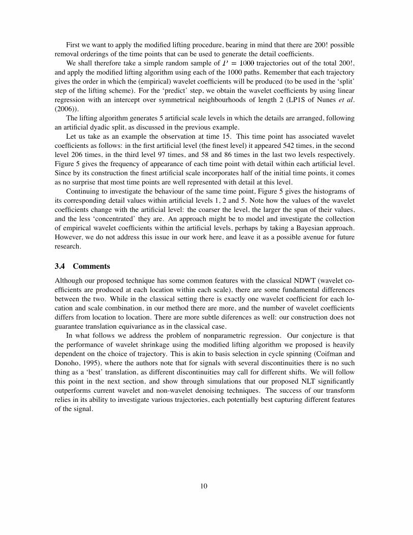
First we want to apply the modified lifting procedure, bearing in mind that there are 200! possibleremoval orderings of the time points that can be used to generate the detail coefficients.

We shall therefore take a simple random sample of trajectories out of the total 200!,and apply the modified lifting algorithm using each of the 1000 paths. Remember that each trajectorygives the order in which the (empirical) wavelet coefficients will be produced (to be used in the ‘split’step of the lifting scheme). For the ‘predict’ step, we obtain the wavelet coefficients by using linearregression with an intercept over symmetrical neighbourhoods of length 2 (LP1S of Nunes et al.(2006)).

The lifting algorithm generates 5 artificial scale levels in which the details are arranged, followingan artificial dyadic split, as discussed in the previous example.

Let us take as an example the observation at time 15. This time point has associated waveletcoefficients as follows: in the first artificial level (the finest level) it appeared 542 times, in the secondlevel 206 times, in the third level 97 times, and 58 and 86 times in the last two levels respectively.Figure 5 gives the frequency of appearance of each time point with detail within each artificial level.Since by its construction the finest artificial scale incorporates half of the initial time points, it comesas no surprise that most time points are well represented with detail at this level.

Continuing to investigate the behaviour of the same time point, Figure 5 gives the histograms ofits corresponding detail values within artificial levels 1, 2 and 5. Note how the values of the waveletcoefficients change with the artificial level: the coarser the level, the larger the span of their values,and the less ‘concentrated’ they are. An approach might be to model and investigate the collectionof empirical wavelet coefficients within the artificial levels, perhaps by taking a Bayesian approach.However, we do not address this issue in our work here, and leave it as a possible avenue for futureresearch.

3.4 Comments

Although our proposed technique has some common features with the classical NDWT (wavelet co-efficients are produced at each location within each scale), there are some fundamental differencesbetween the two. While in the classical setting there is exactly one wavelet coefficient for each lo-cation and scale combination, in our method there are more, and the number of wavelet coefficientsdiffers from location to location. There are more subtle diferences as well: our construction does notguarantee translation equivariance as in the classical case.

In what follows we address the problem of nonparametric regression. Our conjecture is thatthe performance of wavelet shrinkage using the modified lifting algorithm we proposed is heavilydependent on the choice of trajectory. This is akin to basis selection in cycle spinning (Coifman andDonoho, 1995), where the authors note that for signals with several discontinuities there is no suchthing as a ‘best’ translation, as different discontinuities may call for different shifts. We will followthis point in the next section, and show through simulations that our proposed NLT significantlyoutperforms current wavelet and non-wavelet denoising techniques. The success of our transformrelies in its ability to investigate various trajectories, each potentially best capturing different featuresof the signal.

10

Figure 5: Top left, top right, bottom left: histograms of the values of details associated with theobservation at time 15 for artificial levels 1, 2 respectively 5. Bottom right: number of times eachtime point is represented with details within each artificial level. The artificial levels are from finest(1, bottom) to coarsest (5, top). The intensity (darkness) of a pixel corresponds to a higher number ofappearances. White lines extending over all artificial levels correspond to the missing time points.

11

4 Application to nonparametric regression

4.1 Wavelet shrinkage and the NLT

In this section we use wavelet shrinkage for solving the nonparametric regression problem (see section2.4). We first combine our NLT with the wavelet shrinkage technique, then propose an estimator andmove onto characterizing it. Section 4.2 contains the details of the simulation study we used in orderto assess the performance of the proposed estimator, as well as the simulation results.

We embed our NLT in the wavelet shrinkage approach as follows:

1. Select trajectories, out of the paths that the modified lifting algorithm can pos-sibly follow. Each path , where , is in fact a vector containing a random permutationof the locations .

2. For each path, say with : decompose into details by using our modified liftingalgorithm which removes the points in the order specified by , shrink/threshold the detailsusing a chosen shrinkage technique, and then invert the transform.The obtained signal, let us denote it by , estimates the unknown function at locations.

3. Compute an averaged estimator of , , by combining all the estimators of :

(6)

The average estimator is our proposed estimator for , and in what follows we will highlight itsbenefits. Our estimator is similar to the one proposed in cycle spinning, constructed as the average ofestimators corresponding to shifted wavelet bases.

4.1.1 Risk of the aggregate estimator

The performance of is related to the magnitude of its risk (see (5)):

AMSE E E (7)

From (6) it follows that

(8)

which together with (7) gives

AMSE E

E

12

We denote

ACovE E (9)

where , and the notation ACovE stands for Average ‘Covariance’ Error. Should the esti-mators , of be unbiased, this would be indeed the average covariance of the error functions.

Note thatACovE ACovE

Using the notation above, equation (9) can be re-written as

AMSE AMSE ACovE (10)

Equation (10) uncovers the way in which the risks of the individual estimators ,combine in the risk of the aggregate estimator , with the second term in the sum highlighting that the‘covariance’ structure of estimators also plays a role in obtaining the overall risk.

4.1.2 Trajectory selection

As already mentioned, we conjecture that some permutations/trajectories, yield better estimators forthan others. Of course, the order of point removal in conjuction with the actual structure of locationswill influence the quality of the estimator , as measured by its risk. However, their relationship isvery intricate and in what follows we shall try to devise a way through which we can select out of agiven set of paths, the ones which we suspect to give better results. Hence we ask the question: howcan we estimate which trajectories , are likely to produce good estimators of ?

Because of the nature of our modified lifting algorithm, we cannot take a cross-validation approachin order to select the ‘best’ permutation: when we remove an initial data point (location), the trajectoryneeds to be altered too, as it may contain a location no longer available. Therefore, there will be noconsistency even when trying to assess the same path.

For a path , , we want to estimate the average square error corresponding to ,ASE , where is the estimated value of , obtainedas described in the beginning of section 4.1.

We propose to approximate ASE by

ASE (11)

where is the averaged estimator given by (6).In effect, we replace the unknown signal by an averaged estimate . It is well known that average

basis estimators perform better than individual ones, which is also backed up by our simulations (seeTable 1).

Let us work out now

E ASE E

13

hence

E ASE E E

E

from which it follows that

E ASE AMSE AMSE E

Using the notation in (9), and equation (10), the above formula becomes

E ASE AMSE AMSE

ACovE ACovE

The equation above gives a heuristic justification for usingASE to approximate ASE ,as large , bounded average mean square errors and negligible average covariance errors would im-ply that E ASE approximates AMSE . The value of ASE will be used forassessing how well the trajectory performs. Based on it we shall estimate from a set of givenpermutations which are the ones with better performance. This leads us to the idea of trying to buildbetter permutations from a set of random ones.

4.1.3 Generate ‘well-behaved’ trajectories

We shall employ a strategy similar to that encountered in genetic algorithms (GA) (Lucasius andKateman, 1993, 1994), which we adapt to the characteristics of our problem. Simply put, a GAconstructs new offspring generations starting from a set of individuals.

In our case the individuals are the trajectories. Start from a collection of randomly chosenindividuals, viewed as the ‘parents’, and build the ‘next generation’. The algorithm for creating the‘next generation’ of paths is as follows:

Retain only a certain percentage of the current generation, say (known as ‘elitism’), ac-cording to a selection criterion. In our case we choose the criterion to be minimization of theapproximated average square error of the estimator associated to each path . Therefore,the selected trajectories correspond to the lowest approximated average square errors.

Then ‘children’ are created by randomly using crossovers of the parents (i.e. putting togethertwo randomly selected sections of the ‘parents’). Where in a child two sequences of the parentsmeet that have common locations, we ignore the second appearances and randomly fill the lastentries with the missing locations.

The last step in defining the children is to mutate some locations in each child (trajectory). Thisstep ensures that in the long run the whole space of sequences would be visited.

14

Now we have the ‘new generation’ and the algorithm can be re-iterated.From its construction, the algorithm seeks to create trajectories that minimize the approximated

average square errors. Should we be able to compute the exact average square errors correspondingto the trajectories, the algorithm would progressively yield, at each step, new paths associated toestimators with lowest risks. As only an approximation of the true (unknown) error is available, theresults of the GA are themselves only estimates of the ‘best’ trajectories.

In the next section we describe the results from the simulation study through which we investigatethe denoising performance of our proposed NLT teamed with empirical Bayes shrinkage. We comparethe estimated risk of the averaged estimator to the estimated risk of the estimator obtained byusing single selected trajectories . We also compare the performance of our aggregate estimator tothat of the estimator obtained when the order of point removal is established as in Jansen et al. (2004)(see also Nunes et al. (2006) for denoising performance of these estimators). We then investigate theefficiency of our proposed approximation for the average square error in selecting ‘better’ paths froma given set. Finally, we investigate whether we can improve on an initial random population of pathsby constructing ‘good’ paths using a GA approach.

4.2 Simulation study

4.2.1 Setting up the study

In order to assess the denoising performance of our proposed NLT, we shall choose some test functionswhich will be sampled, and then simulate noisy versions from these samples.

Test functions. The behaviour of our algorithm will be tested on the functions Blocks, Bumps,HeaviSine and Doppler introduced by Donoho and Johnstone (1994), which attempt to modelvarious signals that arise in practice, and on the Ppoly function introduced by Nason and Sil-verman (1994). Let be a test function, , sampled at locations . Toensure comparability with other studies, such as Nunes et al. (2006), Barber and Nason (2004),we shall first normalize the test signals by var , for all . For ease ofnotation, we will refer to the normalized signal as , rather than change its notation.

Grid locations. Construct the locations by starting from a regular grid of length which spans, and then jittering the locations following a uniform distribution on the interval

, as in Nunes et al. (2006).

Noise level. We generate noise by setting the signal-to-noise ratio (SNR)var (remember that by construction var ).The noise obtained is added to the signal, creating a noisy version of it, , where

.

Denoising strategy. We follow the procedure described in section 4.1 in order to remove the noisefrom . First, randomly select a set of paths and apply the modified lifting transformtimes, such that the algorithm follows each of the proposed trajectories. As Nunes et al. (2006)showed, algorithms with adaptive prediction outperform non-adaptive ones, hence we use anadaptive prediction step in our algorithm (more exactly AP1S from Nunes et al. (2006)). Thesignal will be fully decomposed into wavelet coefficients, hence in effect our proposed algo-rithm will produce sets of (noise contaminated) details.

15

In order to remove the noise, we threshold each set of details using an empirical Bayesian proce-dure, implemented in EBayesThresh (Johnstone and Silverman, 2004a,b, 2005), with posteriormedian threshold, adapted to suit the characteristics of the lifting algorithm (Nunes et al., 2006).Following the shrinkage procedure, each algorithm is inverted, and the averaged estimator iscomputed.

4.2.2 Assessing performance

For assessing the performance of our algorithm, we repeat our denoising procedure times for eachtest signal– i.e. generate (irregular) grids , sample the test function on eachgrid and add noise; let us denote the noisy signals by , and generate for each of themrandom trajectories; compute using the method previously described an aggregate estimator of the

initial signal, hence obtain .We can therefore obtain a measure of the overall accuracy of our estimating procedure, quantified

by the (estimated) average mean square error,

amseperm (12)

where ‘perm’ stands for permutation.For each noisy signal , we shall also apply the lifting algorithm where the path is

chosen according to the grid configuration as in Jansen et al. (2004) (JNS), and obtain estimatesJNS JNS of . We shall refer to these as ‘JNS’ estimates of , and quantify their perfor-

mance by amseJNS computed as in equation (12), with JNS instead of , for all .In our study we use signals of length , runs and various values for .

4.2.3 Simulation results

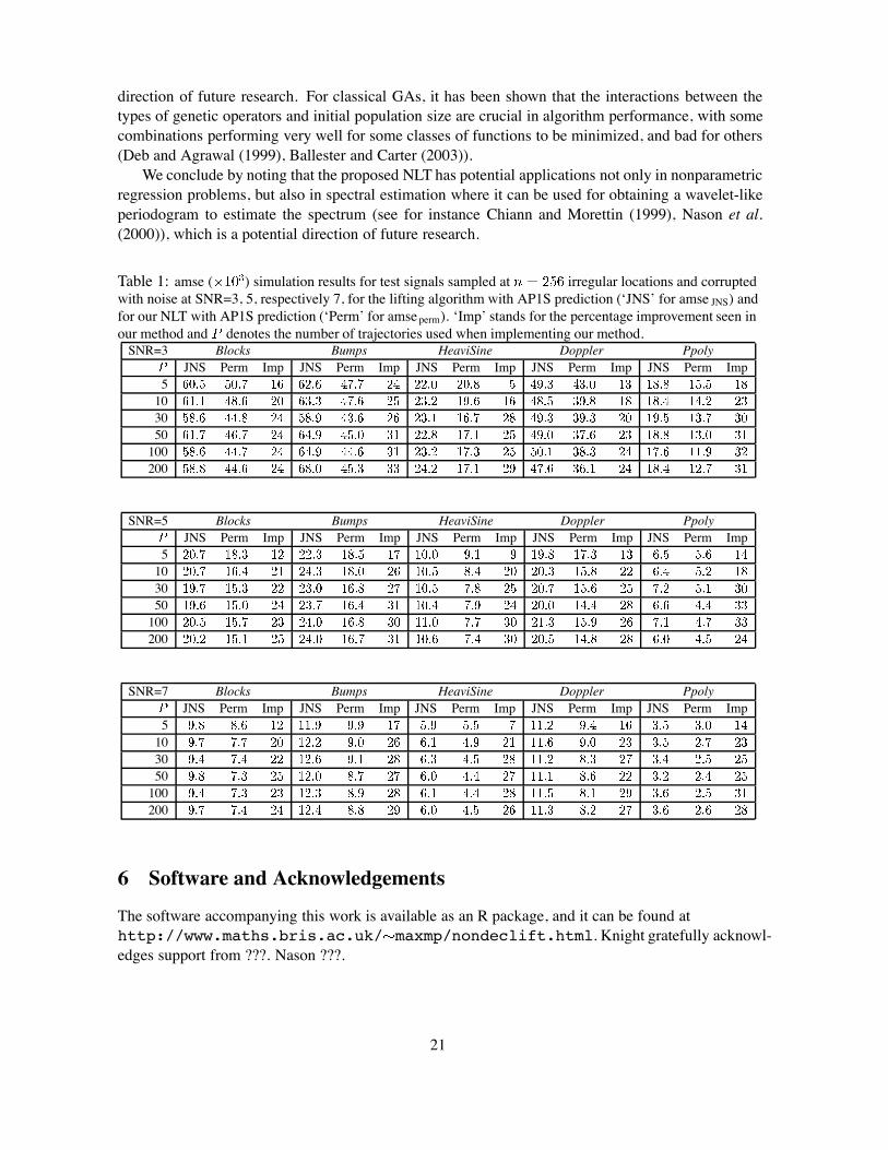
Number of permutations. Table 1 compares the performance of the estimators obtained by our NLTversus the performance of the estimators obtained by using AP1S of Nunes et al. (2006). We chosethis comparison as denoising using AP1S outperforms classical wavelet and non-wavelet denoisingtechniques capable of working on irregular data as Nunes et al. (2006) demonstrate.

Upon analysis of the results in Table 1, we conclude that our method significantly outperformsthe successful adaptive lifting algorithm proposed by Nunes et al. (2006). This does not come as amajor surprise, as, like in cycle spinning, we are in effect averaging the results obtained over several( ) representations, rather than taking just one. Our method does improve on the reported resultsobtained through AN1 (Nunes et al., 2006) as well.

Inspection of the ASE for individual trajectories reveals a large variability. However,by averaging over several ( ) estimators, the risk of the resulting aggregate estimator is usually lowerthan the individual risks. Out of the selected trajectories, the JNS path consistently (and reassuringly,as far as previous work is concerned) appears to perform well.

As hypothesized, amseperm improves with the increasing number of trajectories, regardless ofthe signal or of the level of contaminating noise. For increasing from 1 to 20–30, the amsepermdecreases, after which the increase in the number of paths does not affect the performance of theaveraged estimator to the same extent. Based on these results we decided to use paths fromnow onwards.

16

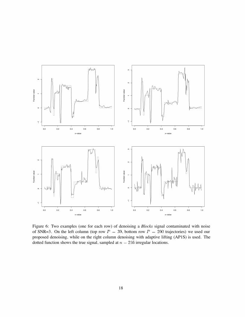
Figure 6 is an example of the outcome from our denoising approach (‘perm’) versus that wherethe signal is decomposed by (JNS type) adaptive lifting. Our estimate is visually smoother (especiallyfor the example on the second row which uses higher , i.e. more trajectories) and it performs betterat the points where sharp discontinuities occur. Smoothing effects have also been observed for theestimators of cycle spinning (Coifman and Donoho, 1995).

The variation displayed in performance between various paths is the reason behind our next step:estimate which paths out of a given set correspond to good estimators.Selection of trajectories. We start with a set of trajectories, out of which we choose

those % estimators corresponding to the smallest estimated risks (ASE). The simulated data showsthat there are good correlation indices betweenASE and ASE (over ), so our proposed approxi-mation for the average square error was a reasonable choice.

Simulations show that values of in the region of 20–30% are sufficient to bring down amsepermfor all tested signals, despite the fact that fewer trajectories are used. For instance when , forBlocks the value of amseperm decreases from 45.6 to 43.6, for Bumps from 45.3 to 44.7, for HeaviSinefrom 16.7 to 16.1, while for Doppler 36.7 is brought down to 36.3 and for Ppoly 12.7 goes down to11.7. Numerically, the decrease in amseperm is probably not significant enough to justify the compu-tational expense, so for the purpose of the averaged estimator we do not think that such a procedureis necessary. For other problems, it could be very helpful to know which trajectories are likely toperform better and which ones should be avoided.

For reference, we also randomly selected % trajectories out of the initial set, and computed theestimated risk of the corresponding averaged estimator. Indeed the risk is consistently higher than forthe estimator obtained by our selection criterion.

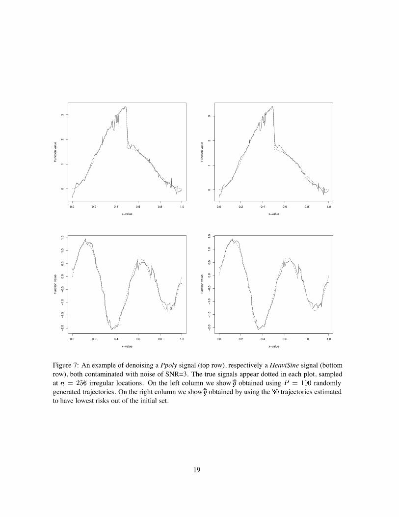
Figure 7 shows that while numerically the difference between the two aggregate estimators (basedon a random choice of paths, or on a selection of trajectories out of the initial set, respectively) issmall, visually the estimator does improve by trajectory selection even though fewer permutationsare used for computing it. The estimators in the right column of Figure 7 appear to be smoother anddisplay less artifacts than the ones in the left column.Trajectory construction. We conclude our investigation by reporting the results obtained when

trying to generate ‘well-behaved’ trajectories by using a GA type approach. We used elitism of, as recommended by Lucasius and Kateman (1993, 1994). The mutation chance was set

at , which ensures that enough mutations occur at each generation to eventually cover the wholepermutation space, while not completely changing the trajectories at each step.

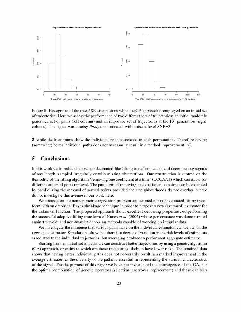
The simulation results can be found in Table 2, which gives the amseperm values corresponding tothe th, th and th generations obtained by the GA approach. Note that a marked improvement(over 10%) in the aggregate estimator is obtained only for Ppoly, while Bumps shows no benefit fromthe usage of the GA. Generally, increasing the number of generations does not appear to heavilyinfluence the results. We account this by the following observation: if we have a set of trajectorieswith low risks, but the paths themselves are very similar, the risk of the aggregate estimator does notget much lower by combining them. Interestingly, the same number of fundamentally different pathswith higher individual risks can yield an aggregate estimator with a much lower risk. Maybe thisshould not come as a complete surprise since it is precisely the diversity of the paths that ‘catches’ thevarious characteristics of the signal.

Figure 8 shows that the distribution of the true average squared errors of individual permutationsbecomes more skewed to the left with the application of the GA. This indicates that the application ofthe GA effectively contributes to lowering the individual risks associated to each path in the trajectoryset.

We should however remember that Table 2 summarizes the behaviour of the averaged estimator,

17

0.0 0.2 0.4 0.6 0.8 1.0

−10

12

x−value

Func

tion

valu

e

0.0 0.2 0.4 0.6 0.8 1.0−1

01

23

x−value

Func

tion

valu

e

0.0 0.2 0.4 0.6 0.8 1.0

−10

12

x−value

Func

tion

valu

e

0.0 0.2 0.4 0.6 0.8 1.0

−10

12

3

x−value

Func

tion

valu

e

Figure 6: Two examples (one for each row) of denoising a Blocks signal contaminated with noiseof SNR=3. On the left column (top row , bottom row trajectories) we used ourproposed denoising, while on the right column denoising with adaptive lifting (AP1S) is used. Thedotted function shows the true signal, sampled at irregular locations.

18

0.0 0.2 0.4 0.6 0.8 1.0

01

23

x−value

Func

tion

valu

e

0.0 0.2 0.4 0.6 0.8 1.00

12

3x−value

Func

tion

valu

e

0.0 0.2 0.4 0.6 0.8 1.0

−2.0

−1.5

−1.0

−0.5

0.0

0.5

1.0

1.5

x−value

Func

tion

valu

e

0.0 0.2 0.4 0.6 0.8 1.0

−2.0

−1.5

−1.0

−0.5

0.0

0.5

1.0

1.5

x−value

Func

tion

valu

e

Figure 7: An example of denoising a Ppoly signal (top row), respectively a HeaviSine signal (bottomrow), both contaminated with noise of SNR=3. The true signals appear dotted in each plot, sampledat irregular locations. On the left column we show obtained using randomlygenerated trajectories. On the right column we show obtained by using the trajectories estimatedto have lowest risks out of the initial set.

19

Representation of the initial set of permutations

True ASEs (*1000) corresponding to the initial set of trajectories

Freq

uenc

y

0 20 40 60 80 100 120

050

010

0015

0020

00

Representation of the set of permutations at the 10th generation

True ASEs (*1000) corresponding to the trajectories after 10 GA iterations

Freq

uenc

y

0 20 40 60 80 100 120

050

010

0015

0020

00

Figure 8: Histograms of the true ASE distributions when the GA approach is employed on an initial setof trajectories. Here we assess the performance of two different sets of trajectories: an initial randomlygenerated set of paths (left column) and an improved set of trajectories at the th generation (rightcolumn). The signal was a noisy Ppoly contaminated with noise at level SNR=3.

, while the histograms show the individual risks associated to each permutation. Therefore having(somewhat) better individual paths does not necessarily result in a marked improvement in .

5 Conclusions

In this work we introduced a new nondecimated-like lifting transform, capable of decomposing signalsof any length, sampled irregularly or with missing observations. Our construction is centred on theflexibility of the lifting algorithm ‘removing one coefficient at a time’ (LOCAAT) which can allow fordifferent orders of point removal. The paradigm of removing one coefficient at a time can be extendedby parallelizing the removal of several points provided their neighbourhoods do not overlap, but wedo not investigate this avenue in our work here.

We focused on the nonparametric regression problem and teamed our nondecimated lifting trans-form with an empirical Bayes shrinkage technique in order to propose a new (averaged) estimator forthe unknown function. The proposed approach shows excellent denoising properties, outperformingthe successful adaptive lifting transform of Nunes et al. (2006) whose performance was demonstratedagainst wavelet and non-wavelet denoising methods capable of working on irregular data.

We investigate the influence that various paths have on the individual estimators, as well as on theaggregate estimator. Simulations show that there is a degree of variation in the risk levels of estimatorsassociated to the individual trajectories, but averaging produces a performant aggregate estimator.

Starting from an initial set of paths we can construct better trajectories by using a genetic algorithm(GA) approach, or estimate which are those trajectories likely to have lower risks. The obtained datashows that having better individual paths does not necessarily result in a marked improvement in theaverage estimator, as the diversity of the paths is essential in representing the various characteristicsof the signal. For the purpose of this paper we have not investigated the convergence of the GA, northe optimal combination of genetic operators (selection, crossover, replacement) and these can be a

20

direction of future research. For classical GAs, it has been shown that the interactions between thetypes of genetic operators and initial population size are crucial in algorithm performance, with somecombinations performing very well for some classes of functions to be minimized, and bad for others(Deb and Agrawal (1999), Ballester and Carter (2003)).

We conclude by noting that the proposed NLT has potential applications not only in nonparametricregression problems, but also in spectral estimation where it can be used for obtaining a wavelet-likeperiodogram to estimate the spectrum (see for instance Chiann and Morettin (1999), Nason et al.(2000)), which is a potential direction of future research.

Table 1: amse ( ) simulation results for test signals sampled at irregular locations and corruptedwith noise at SNR=3, 5, respectively 7, for the lifting algorithm with AP1S prediction (‘JNS’ for amse JNS) andfor our NLT with AP1S prediction (‘Perm’ for amseperm). ‘Imp’ stands for the percentage improvement seen inour method and denotes the number of trajectories used when implementing our method.SNR=3 Blocks Bumps HeaviSine Doppler Ppoly

JNS Perm Imp JNS Perm Imp JNS Perm Imp JNS Perm Imp JNS Perm Imp5103050100200

SNR=5 Blocks Bumps HeaviSine Doppler PpolyJNS Perm Imp JNS Perm Imp JNS Perm Imp JNS Perm Imp JNS Perm Imp

5103050100200

SNR=7 Blocks Bumps HeaviSine Doppler PpolyJNS Perm Imp JNS Perm Imp JNS Perm Imp JNS Perm Imp JNS Perm Imp

5103050100200

6 Software and Acknowledgements

The software accompanying this work is available as an R package, and it can be found athttp://www.maths.bris.ac.uk/ maxmp/nondeclift.html. Knight gratefully acknowl-edges support from ???. Nason ???.

21

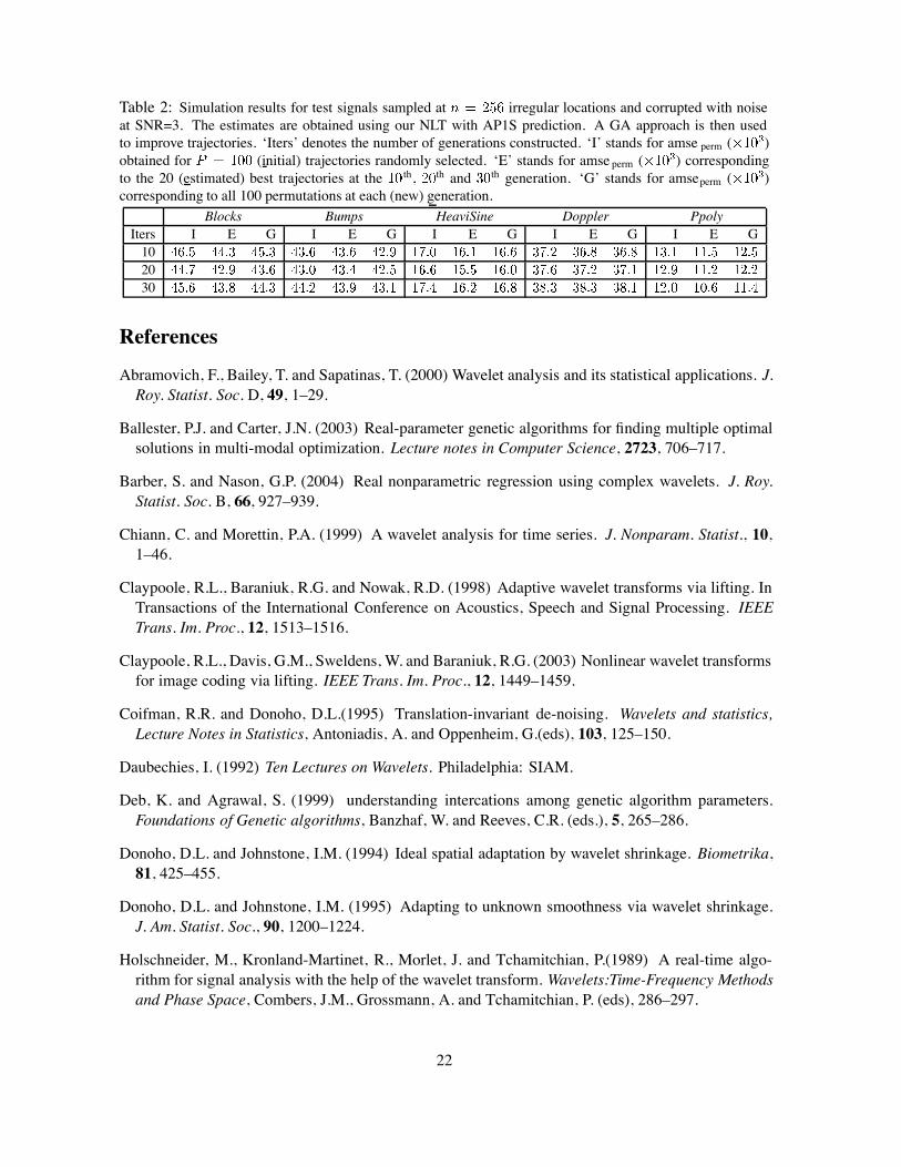
Table 2: Simulation results for test signals sampled at irregular locations and corrupted with noiseat SNR=3. The estimates are obtained using our NLT with AP1S prediction. A GA approach is then usedto improve trajectories. ‘Iters’ denotes the number of generations constructed. ‘I’ stands for amse perm ( )obtained for (initial) trajectories randomly selected. ‘E’ stands for amse perm ( ) correspondingto the 20 (estimated) best trajectories at the th, th and th generation. ‘G’ stands for amseperm ( )corresponding to all 100 permutations at each (new) generation.

Blocks Bumps HeaviSine Doppler PpolyIters I E G I E G I E G I E G I E G102030

References

Abramovich, F., Bailey, T. and Sapatinas, T. (2000) Wavelet analysis and its statistical applications. J.Roy. Statist. Soc. D, 49, 1–29.

Ballester, P.J. and Carter, J.N. (2003) Real-parameter genetic algorithms for finding multiple optimalsolutions in multi-modal optimization. Lecture notes in Computer Science, 2723, 706–717.

Barber, S. and Nason, G.P. (2004) Real nonparametric regression using complex wavelets. J. Roy.Statist. Soc. B, 66, 927–939.

Chiann, C. and Morettin, P.A. (1999) A wavelet analysis for time series. J. Nonparam. Statist., 10,1–46.

Claypoole, R.L., Baraniuk, R.G. and Nowak, R.D. (1998) Adaptive wavelet transforms via lifting. InTransactions of the International Conference on Acoustics, Speech and Signal Processing. IEEETrans. Im. Proc., 12, 1513–1516.

Claypoole, R.L., Davis, G.M., Sweldens, W. and Baraniuk, R.G. (2003) Nonlinear wavelet transformsfor image coding via lifting. IEEE Trans. Im. Proc., 12, 1449–1459.

Coifman, R.R. and Donoho, D.L.(1995) Translation-invariant de-noising. Wavelets and statistics,Lecture Notes in Statistics, Antoniadis, A. and Oppenheim, G.(eds), 103, 125–150.

Daubechies, I. (1992) Ten Lectures on Wavelets. Philadelphia: SIAM.

Deb, K. and Agrawal, S. (1999) understanding intercations among genetic algorithm parameters.Foundations of Genetic algorithms, Banzhaf, W. and Reeves, C.R. (eds.), 5, 265–286.

Donoho, D.L. and Johnstone, I.M. (1994) Ideal spatial adaptation by wavelet shrinkage. Biometrika,81, 425–455.

Donoho, D.L. and Johnstone, I.M. (1995) Adapting to unknown smoothness via wavelet shrinkage.J. Am. Statist. Soc., 90, 1200–1224.

Holschneider, M., Kronland-Martinet, R., Morlet, J. and Tchamitchian, P.(1989) A real-time algo-rithm for signal analysis with the help of the wavelet transform. Wavelets:Time-Frequency Methodsand Phase Space, Combers, J.M., Grossmann, A. and Tchamitchian, P. (eds), 286–297.

22

Jansen, M., Nason, G.P. and Silverman, B.W. (2001) Scattered data smoothing by empirical Bayesianshrinkage of second generation wavelet coefficients. In Unser, M. and Aldroubi, A. (eds) Waveletapplications in signal and image processing, Proceedings of SPIE, 4478, 87–97.

Jansen, M., Nason, G.P. and Silverman, B.W. (2004) Multivariate nonparametric regression usinglifting. Technical Report 04:17, Statistics Group, Department of Mathematics, University of Bristol,UK.

Johnstone, I.M. and Silverman, B.W. (2004a) Needles and hay in haystacks: Empirical Bayes esti-mates of possibly sparse sequences. Ann. Statist., 32, 1594–1649.

Johnstone, I.M. and Silverman, B.W. (2004b) EbayesThresh: R programs for Empirical Bayes thresh-olding. J. Statist. Soft., 12, 1–38.

Johnstone, I.M. and Silverman, B.W. (2005) Empirical Bayes selection of wavelet thresholds. Ann.Statist., 33, (to appear).

Lee, C.S., Lee, C.K. and Yoo, K.Y. (2000) New lifting based structure for undecimated wavelettransform. Electronics Letters, 36, 1894–1895.

Lucasius, C.B. and Kateman, G. (1993) Understanding and using genetic algorithms– Part 1. Con-cepts, properties and context. Chemometrics and Intelligent Laboratory Systems, 19, 1–33.

Lucasius, C.B. and Kateman, G. (1994) Understanding and using genetic algorithms– Part 2. Repre-sentation, configuration and hybridization. Chemometrics and Intelligent Laboratory Systems, 25,99–145.

Nason, G.P. and Silverman, B.W. (1994) The discrete wavelet transform in S. J. Comput. Graph.Statist., 3, 163–191.

Nason, G.P. and Silverman, B.W. (1995) The Stationary wavelet transform and some statistical ap-plications. Wavelets and Statistics, Lecture Notes in Statistics, Antoniadis, A. and Oppenheim, G.(eds), 103, 281–300.

Nason, G.P., von Sachs, R. and Kroisandt, G. (2000) Wavelet processes and adaptive estimation ofthe evolutionary wavelet spectrum. J. Roy. Statist. Soc. B, 62, 271–292.

Nunes, M.A., Knight, M.I. and Nason, G.P. (2006) Adaptive lifting in nonparametric regression.Statist. Comput., 16, 143–159.

Nunes, M.A. and Nason, G.P. (2005) Stopping time in adaptive lifting. Technical Report 05:15,Statistics Group, Department of Mathematics, University of Bristol, UK.

Percival, D.B. (1996) On estimation of the wavelet variance. Biometrika, 82, 619–631.

Percival, D.B. and Walden, A.T. (2000) Wavelet Methods for Time Series Analysis. Cambridge Uni-versity Press, Cambridge.

Pesquet, J.C., Krim, H. and Carfantan, H. (1996) Time invariant orhtonormal wavelet representations.IEEE Trans. Signal Proc., 44, 1964–1970.

Piella, G. and Heijmans, H.J.A.M. (2002) Adaptive lifting schemes with perfect reconstruction. IEEETrans. Sig. Proc., 50, 1620–1630.

23

Sweldens, W. (1996) Wavelets and the lifting scheme: A 5 minute tour. Z. Angew. Math. Mech., 76,41–44.

Sweldens, W. (1998) The lifting scheme: a construction of second generation wavelets. SIAM J.Math. Anal., 29, 511–546.

Trappe, W. and Liu, K.J.R. (2000) Denoising via adaptive lifting schemes. In Proceedings ofSPIE, Wavelet applications in signal and image processing VIII, Aldroubi, A., Laine, M.A. andUnser, M.A. (eds), 4119, 302–312.

Vidakovic, B. (1999) Statistical modeling by wavelets. Wiley: New York.

24