A non-stiff boundary integral method for internal waves

A non-stiff boundary integral method for internal waves

NJIT, 4 June 2013

Oleksiy Varfolomiyevadvisor Michael Siegel

Wednesday, June 19, 13

Motivation


Motivation

Develop a model and a numerical method that can be efficiently applied to study the motion of internal waves for doubly periodic interfacial flows with surface tension.


Outline


Outline

•Model Description


Outline


•Linear Stability Analysis


Outline



•Discretization


Outline



•Discretization

•Numerical Experiment


⇤! p(�) : p(�) = minq⇥Pk

max�⇥[�min,�max]

��1⌅�� q(�)

�� (41)

We used Wolfram Mathematica intrinsic function MiniMaxApproximation toobtain p(�). The next figure shows the approximation error

10 100 1000 104

10!15

10!14

10!13

10!12

10!11

To obtain grid steps we rewrite obtained approximation of the impedancefunction in the form of continued fraction (12). We proceed with Euclidean typealgorithm with 2k polynomial divisions, i.e.

p(�) =ck�1�k�1 + ck�2�k�2 + · · ·+ c0dk�k + dk�1�k�1 + · · ·+ d0

(42)

=1

dk�k+dk�1�k�1+···+d0ck�1�k�1+ck�2�k�2+···+c0

=1

dkck�1

�+

✓dk�1�

dkck�2ck�1

◆�k�1+···+

✓d1�

dkc0ck�1

◆�+d0

ck�1�k�1+ck�2�k�2+···+c0

,

ˆ d

Model Description


⇤! p(�) : p(�) = minq⇥Pk


��1⌅�� q(�)

�� (41)


10 100 1000 104

10!15

10!14

10!13

10!12

10!11



(42)

=1

dk�k+dk�1�k�1+···+d0ck�1�k�1+ck�2�k�2+···+c0

=1

dkck�1

�+

✓dk�1�

dkck�2ck�1

◆�k�1+···+

✓d1�

dkc0ck�1

◆�+d0

ck�1�k�1+ck�2�k�2+···+c0

,

ˆ d

Model DescriptionEvolution of the interface between two immiscible, inviscid, incompressible, irrotational fluids of different density in 3D.


⇤! p(�) : p(�) = minq⇥Pk


��1⌅�� q(�)

�� (41)


10 100 1000 104

10!15

10!14

10!13

10!12

10!11



(42)

=1

dk�k+dk�1�k�1+···+d0ck�1�k�1+ck�2�k�2+···+c0

=1

dkck�1

�+

✓dk�1�

dkck�2ck�1

◆�k�1+···+

✓d1�

dkc0ck�1

◆�+d0

ck�1�k�1+ck�2�k�2+···+c0

,

ˆ d

Model Description

Motion of the fluids is driven by

Evolution of the interface between two immiscible, inviscid, incompressible, irrotational fluids of different density in 3D.


⇤! p(�) : p(�) = minq⇥Pk


��1⌅�� q(�)

�� (41)


10 100 1000 104

10!15

10!14

10!13

10!12

10!11



(42)

=1

dk�k+dk�1�k�1+···+d0ck�1�k�1+ck�2�k�2+···+c0

=1

dkck�1

�+

✓dk�1�

dkck�2ck�1

◆�k�1+···+

✓d1�

dkc0ck�1

◆�+d0

ck�1�k�1+ck�2�k�2+···+c0

,

ˆ d

Model Description

➡ Gravity




⇤! p(�) : p(�) = minq⇥Pk


��1⌅�� q(�)

�� (41)


10 100 1000 104

10!15

10!14

10!13

10!12

10!11



(42)

=1

dk�k+dk�1�k�1+···+d0ck�1�k�1+ck�2�k�2+···+c0

=1

dkck�1

�+

✓dk�1�

dkck�2ck�1

◆�k�1+···+

✓d1�

dkc0ck�1

◆�+d0

ck�1�k�1+ck�2�k�2+···+c0

,

ˆ d

Model Description

➡ Gravity

➡ Surface Tension




⇤! p(�) : p(�) = minq⇥Pk


��1⌅�� q(�)

�� (41)


10 100 1000 104

10!15

10!14

10!13

10!12

10!11



(42)

=1

dk�k+dk�1�k�1+···+d0ck�1�k�1+ck�2�k�2+···+c0

=1

dkck�1

�+

✓dk�1�

dkck�2ck�1

◆�k�1+···+

✓d1�

dkc0ck�1

◆�+d0

ck�1�k�1+ck�2�k�2+···+c0

,

ˆ d

Model Description

➡ Gravity

➡ Surface Tension

➡ Prescribed far-field pressure gradient




Governing Equations

1 Model problem

Consider the following boundary value problem: Laplace equation on a semi-infinite strip with the given Neumann data on the left boundary and Dirichletdata elsewhere

�⌅2w(x, y)

⌅y2� ⌅2w(x, y)

⌅x2= 0, (x, y) ⌅ [0,⇤)⇥ [0, 1], (1)

⌅w

⌅x(0, y) = �⇤(y), y ⌅ [0, 1], (2)

w|x=⇥ = 0, (3)

w(x, 0) = 0, w(x, 1) = 0, x ⌅ [0,⇤). (4)

Assume

⇤(y) =m�

i=1

ai sin(i⇥y) (5)

The above problem can be studied as a problem

Aw(x)� d2w(x)

dx2= 0, x ⌅ [0,⇤) (6)

dw

dx(x = 0) = �⇤ (7)

w|x=⇥ = 0, (8)

where A = � �2

�y2 is defined on span{sin (⇥y), . . . , sin (m⇥y)}, spA =

{⇥2, . . . , (m⇥)2}. We can obtain Dirichlet data on the left boundary using

Neumann-to-Dirichlet map. Equation (6) gives Aw(x) = d2w(x)dx2 , therefore

�dw(x)dx = A

12w(x) and now we can use given in (7) Neumann data to get at

x = 0w(0) = f(A)⇤,

here f(�) = �� 12 is impedance function.

2


Governing Equations

1 Model problem


�⌅2w(x, y)

⌅y2� ⌅2w(x, y)

⌅x2= 0, (x, y) ⌅ [0,⇤)⇥ [0, 1], (1)

⌅w

⌅x(0, y) = �⇤(y), y ⌅ [0, 1], (2)

w|x=⇥ = 0, (3)

w(x, 0) = 0, w(x, 1) = 0, x ⌅ [0,⇤). (4)

Assume

⇤(y) =m�

i=1

ai sin(i⇥y) (5)


Aw(x)� d2w(x)

dx2= 0, x ⌅ [0,⇤) (6)

dw

dx(x = 0) = �⇤ (7)

w|x=⇥ = 0, (8)

where A = � �2




�dw(x)dx = A


x = 0w(0) = f(A)⇤,


2

The interface S is parametrized by


Governing Equations

1 Model problem


�⌅2w(x, y)

⌅y2� ⌅2w(x, y)

⌅x2= 0, (x, y) ⌅ [0,⇤)⇥ [0, 1], (1)

⌅w

⌅x(0, y) = �⇤(y), y ⌅ [0, 1], (2)

w|x=⇥ = 0, (3)

w(x, 0) = 0, w(x, 1) = 0, x ⌅ [0,⇤). (4)

Assume

⇤(y) =m�

i=1

ai sin(i⇥y) (5)


Aw(x)� d2w(x)

dx2= 0, x ⌅ [0,⇤) (6)

dw

dx(x = 0) = �⇤ (7)

w|x=⇥ = 0, (8)

where A = � �2




�dw(x)dx = A


x = 0w(0) = f(A)⇤,


2


The fluid velocities are governed by the Bernoulli’s law


Governing Equations

1 Model problem


�⌅2w(x, y)

⌅y2� ⌅2w(x, y)

⌅x2= 0, (x, y) ⌅ [0,⇤)⇥ [0, 1], (1)

⌅w

⌅x(0, y) = �⇤(y), y ⌅ [0, 1], (2)

w|x=⇥ = 0, (3)

w(x, 0) = 0, w(x, 1) = 0, x ⌅ [0,⇤). (4)

Assume

⇤(y) =m�

i=1

ai sin(i⇥y) (5)


Aw(x)� d2w(x)

dx2= 0, x ⌅ [0,⇤) (6)

dw

dx(x = 0) = �⇤ (7)

w|x=⇥ = 0, (8)

where A = � �2




�dw(x)dx = A


x = 0w(0) = f(A)⇤,


2

@�i

@t�r�i ·Xt +

1

2|r�i|2 +

pi⇢i

+ gz = 0 in Di




Governing Equations

1 Model problem


�⌅2w(x, y)

⌅y2� ⌅2w(x, y)

⌅x2= 0, (x, y) ⌅ [0,⇤)⇥ [0, 1], (1)

⌅w

⌅x(0, y) = �⇤(y), y ⌅ [0, 1], (2)

w|x=⇥ = 0, (3)

w(x, 0) = 0, w(x, 1) = 0, x ⌅ [0,⇤). (4)

Assume

⇤(y) =m�

i=1

ai sin(i⇥y) (5)


Aw(x)� d2w(x)

dx2= 0, x ⌅ [0,⇤) (6)

dw

dx(x = 0) = �⇤ (7)

w|x=⇥ = 0, (8)

where A = � �2




�dw(x)dx = A


x = 0w(0) = f(A)⇤,


2

@�i

@t�r�i ·Xt +

1

2|r�i|2 +

pi⇢i

+ gz = 0 in Di


The evolution equation for the free surface S



Boundary Conditions

1 Model problem


�⌅2w(x, y)

⌅y2� ⌅2w(x, y)

⌅x2= 0, (x, y) ⌅ [0,⇤)⇥ [0, 1], (1)

⌅w

⌅x(0, y) = �⇤(y), y ⌅ [0, 1], (2)

w|x=⇥ = 0, (3)

w(x, 0) = 0, w(x, 1) = 0, x ⌅ [0,⇤). (4)

Assume

⇤(y) =m�

i=1

ai sin(i⇥y) (5)


Aw(x)� d2w(x)

dx2= 0, x ⌅ [0,⇤) (6)

dw

dx(x = 0) = �⇤ (7)

w|x=⇥ = 0, (8)

where A = � �2




�dw(x)dx = A


x = 0w(0) = f(A)⇤,


2


Boundary Conditions

1 Model problem


�⌅2w(x, y)

⌅y2� ⌅2w(x, y)

⌅x2= 0, (x, y) ⌅ [0,⇤)⇥ [0, 1], (1)

⌅w

⌅x(0, y) = �⇤(y), y ⌅ [0, 1], (2)

w|x=⇥ = 0, (3)

w(x, 0) = 0, w(x, 1) = 0, x ⌅ [0,⇤). (4)

Assume

⇤(y) =m�

i=1

ai sin(i⇥y) (5)


Aw(x)� d2w(x)

dx2= 0, x ⌅ [0,⇤) (6)

dw

dx(x = 0) = �⇤ (7)

w|x=⇥ = 0, (8)

where A = � �2




�dw(x)dx = A


x = 0w(0) = f(A)⇤,


2

Kinematic boundary condition


Boundary Conditions

1 Model problem


�⌅2w(x, y)

⌅y2� ⌅2w(x, y)

⌅x2= 0, (x, y) ⌅ [0,⇤)⇥ [0, 1], (1)

⌅w

⌅x(0, y) = �⇤(y), y ⌅ [0, 1], (2)

w|x=⇥ = 0, (3)

w(x, 0) = 0, w(x, 1) = 0, x ⌅ [0,⇤). (4)

Assume

⇤(y) =m�

i=1

ai sin(i⇥y) (5)


Aw(x)� d2w(x)

dx2= 0, x ⌅ [0,⇤) (6)

dw

dx(x = 0) = �⇤ (7)

w|x=⇥ = 0, (8)

where A = � �2




�dw(x)dx = A


x = 0w(0) = f(A)⇤,


2


Laplace-Young boundary condition


Boundary Conditions

1 Model problem


�⌅2w(x, y)

⌅y2� ⌅2w(x, y)

⌅x2= 0, (x, y) ⌅ [0,⇤)⇥ [0, 1], (1)

⌅w

⌅x(0, y) = �⇤(y), y ⌅ [0, 1], (2)

w|x=⇥ = 0, (3)

w(x, 0) = 0, w(x, 1) = 0, x ⌅ [0,⇤). (4)

Assume

⇤(y) =m�

i=1

ai sin(i⇥y) (5)


Aw(x)� d2w(x)

dx2= 0, x ⌅ [0,⇤) (6)

dw

dx(x = 0) = �⇤ (7)

w|x=⇥ = 0, (8)

where A = � �2




�dw(x)dx = A


x = 0w(0) = f(A)⇤,


2


Far-field boundary conditions

Laplace-Young boundary condition


Equations to solve


1 Model problem


�⌅2w(x, y)

⌅y2� ⌅2w(x, y)

⌅x2= 0, (x, y) ⌅ [0,⇤)⇥ [0, 1], (1)

⌅w

⌅x(0, y) = �⇤(y), y ⌅ [0, 1], (2)

w|x=⇥ = 0, (3)

w(x, 0) = 0, w(x, 1) = 0, x ⌅ [0,⇤). (4)

Assume

⇤(y) =m�

i=1

ai sin(i⇥y) (5)


Aw(x)� d2w(x)

dx2= 0, x ⌅ [0,⇤) (6)

dw

dx(x = 0) = �⇤ (7)

w|x=⇥ = 0, (8)

where A = � �2




�dw(x)dx = A


x = 0w(0) = f(A)⇤,


2


Linear Stability Analysis


Fourier analysis


Linearized Problem Solution

Remark4t ⇠ (4x)

32


Discretization


Numerical Experiment


Gravity driven flow (Rayleigh-Taylor Instability)

Surface tension interface relaxation

−20

24

68

−20

24

68

−0.8

−0.6

−0.4

−0.2

0

0.2

0.4

0.6

0.8

Numerical Solution

Solution z at T=1 (Implicit method, A=1, dt = 0.1, N=32)

−20

24

68

−20

24

68

−0.4

−0.3

−0.2

−0.1

0

0.1

0.2

0.3

Numerical Solution

Solution z at T=5 (Implicit method, A=0.5, dt = 0.1, N=32)


Numerical Results

Max interface height for lin & num soln. Explicit method, N=32, A=0.

0 0.2 0.4 0.6 0.8 1 1.2 1.4 1.6 1.8 20

0.05

0.1

0.15

0.2

0.25

0.3

0.35

0.4

0.45

0.5

t

max of the lin and num solution zLin and z

lin solnnum soln

Max interface height for lin & num soln. Explicit method, N=32, A=1.

0 0.5 1 1.5 2 2.5 3 3.5 40

0.5

1

1.5

t

max of the lin and num solution zLin and z

lin solnnum soln


Stability

growing unstable modes


Stability ChartLargest stable time step

for the explicit and implicit methods.

4t ⇠ (4x)32


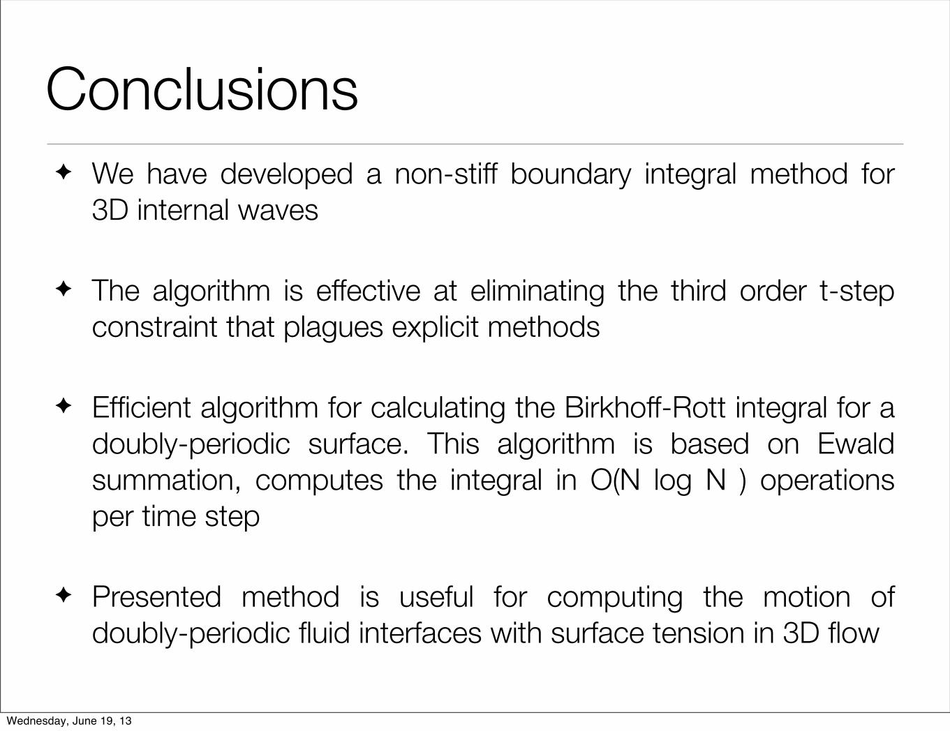
Conclusions✦ We have developed a non-stiff boundary integral method for

3D internal waves

✦ The algorithm is effective at eliminating the third order t-step constraint that plagues explicit methods

✦ Efficient algorithm for calculating the Birkhoff-Rott integral for a doubly-periodic surface. This algorithm is based on Ewald summation, computes the integral in O(N log N ) operations per time step

✦ Presented method is useful for computing the motion of doubly-periodic fluid interfaces with surface tension in 3D flow


A non-stiff boundary integral method for internal waves

Science

Transcript of A non-stiff boundary integral method for internal waves