A New Study On The Impacts Of

Stock Split

Zeng Lei

Nanyang Business School, NTU

Keshab Shrestha

Nanyang Business School, NTU

akeshab@ntu.edu.sg

A New Study On The Impacts Of

Stock Split

ABSTRACT

Stock splits are one of the common phenomena in the stock market. Three main theories are proposed to explain why firms split their stocks. They are liquidity, signaling, and optimal tick size theories. In this paper, we empirically test all three theories using some of the most recent methodologies. We use stock split data from 1962 to 2004. The empirical result is consistent with the signaling hypothesis in the sense that the firm-specific information has been found to decrease after the announcement of stock split. The liquidity has been found to decrease (increase) and the transaction cost has been found to increase (decrease) after the forward (reverse) split. Therefore, for the forward split, the empirical result is not consistent with the liquidity hypothesis which states that the liquidity should increase after the forward stock split. However, the evidence for the reverse split is consistent with the liquidity theory. Even though the increase in transaction cost is consistent with the optimal tick size hypothesis, the decrease in liquidity is not consistent with it. Therefore, the optimal tick size hypothesis is not fully supported by the empirical evidence.

2

1. INTRODUCTION

Stock splits are regular phenomenon in stock markets. There are mainly three theories that explain the reason behind stock split. In this section, we will briefly discuss these theories.

As pointed out by Lakonishok & Lev (1987), stock split is just like “a finer slicing of a given cake”. Since the change in number of shares does not involve changes to the future cash flow, in an efficient market with symmetric information, this event should be irrelevant to the value of the firm. In fact, stock split involves extra costs such as stock issuance taxes, listing fees, and mailing costs etc. (Sosnick (1961)). Despite of the transaction costs, managers are still enthusiastic about splitting their firms’ shares and stock splits are common events in reality. Therefore, the reasons behind stock split has been an interesting research topic in finance. There are three main theories which try to explain the stock split 1.1 Liquidity Theory

The first theory is the liquidity theory (or optimal trading range theory as suggested by Copeland (1979)). It states that there is an optimal price span for the stocks of a company in which trading is the most liquid, and managers adjust the stock price by splitting toward the optimal trading range in order to enhance the liquidity of the stocks. If the price is very high, large investors benefit because of low brokerage cost for their round lots. But small investors are discouraged to trade because of their limited money. Similarly, if the price is very low, large investors are not willing to invest in that stock. Therefore, the optimal price range is to equilibrate the preference of large investors and small investors so that the stock is most liquid.

Baker and Gallagher (1980) presents some evidence in support of this theory. In their

survey of corporate managers’ motivation for stock splits, they find that managers tend to mention an optimal trading range to explain splits. The survey reports that 98% of chief financial officers admit that splits make it easier for small investors to purchase round lot and 94% of them believe that splits increase the number of investors and retain the stock prices in an optimal range.

As to the empirical evidence of stock split on liquidity, Copeland (1979) finds the residual trading volume to decrease after the stock split. Murray (1985) finds the trade volume after stock splits to decreases in short term, but, does not change in long term. Similar results are obtained by Lamoureux & Poon (1987) and Lakonishok & Lev (1987). Desai, Nimalendran & Venkataraman (1998) and Guirao & Sala (2002) and Wulff (2002) find an increase in trading frequency and percentage of trading days, but trade size significantly decreases after stock split.

In some other studies, bid-ask spread is used to indirectly measure the liquidity in the sense that lower bid-ask spread is associated with higher liquidity because it reflects the easiness of converting asset into cash.

Copeland (1979) finds a significant increase in percentage bid-ask spread following a split. However, Murray (1985) finds no evidence of a change in percentage spreads relative to a control sample.

Using NYSE-listed frims, Conroy, Harris, and Benet (1990) find that while absolute spreads significantly decrease following a split, the percentage spreads for the splitting firms increase after the stock split. Similar result is found by Dhar et al. (2003) when using NASDAQ-NMS firms. Desai, Nimalendran & Venkataraman (1998) study the major

1

components of spread (order-processing costs and adverse-information costs) as well as the percentage bid-ask spread. They find both components significantly increase and the percentage spread also increases after the split. Kunz (2002) and Guirao & Sala (2002) also study the quoted percentage spread and effective bid-ask spread for non-US markets. And they also find that quoted percentage spread and effective percentage bid-ask spread increase significantly. Goyenko et al. (2005b) use effective tick suggested by Holden (2004) and round-trip transaction cost estimated using the model suggested by by Lesmond et al. (1999) and Goyenko et al. (2005a) to test the liquidity around stock split over long-time window. By comparing the variable in splitting and control firms, the percent effective spread for splitting firms is only temporarily higher than control sample after splitting and becomes significantly lower than that of control sample in long run. This result presents some evidence of the long-run benefit of split.

In addition to the trading volume and bid-ask spread, price impact of trade is also a good proxy of liquidity. Dhar et al. (2003) have used it to evaluate liquidity. They make use of Barclay & Warner (1993)’s conclusion that medium sized trades mainly impact the stock price. Based on the hypothesis, a lower frequency in medium sized trades implies the improved liquidity. Using the medium sized trade, thier result shows the liquidity increases following the split, but the increase is not significant.

Apart from the use of liquidity proxies to examine the theory, other methods are also applied. Easley, O’hara & Saar (2001) construct a sequential trade model and use maximum likelihood estimation to estimate parameters reflecting the liquidity. They find that the uninformed traders increase after the stock split. This evidence is considered to support the liquidity theory. Muscarella and Vetsuypens (1996) study the ADR ‘solo-splits’ (ADR that splits only in U.S. market). ADR ‘solo-splits’ cannot be motivated by managers’ desire to signal, otherwise, the companies would have split the shares in the domestic market. They find that the liquidity increase significantly after ADR solo-splits where liquidity is measured by dollar trading volume, number of trades and liquidity premium. Dennis (2003) also disentangle the signaling effect from the liquidity effect of stock splits by studying the Nasdaq-100 Index Tracking Stock. Because the index is a market-capitalization weighted index of the 100 largest stocks on the Nasdaq, manager of the trust can not access the information of each stock in the index and signaling effect is excluded during the split. Various liquidity measures are examined for the 2-for-1 split of Nasdaq-100 Index Tracking Stock. He find that while daily turnover does not change and the relative bid-ask spread increases, the trading frequency, the share volume, and the dollar-volume of small trades all increase after the split. He interprets those results as improved liquidity.

In summary, the evidence on the liquidity impact of stock split is mixed. The adjusted trade volume has been generally found to decrease and the percentage bid-ask spread is usually found to increase after the split. However, in some cases, the trading frequency has been found to increase. Therefore, more studies are needed to examine the liquidity theory. 1.2 The Signaling Theory

The second explanation for the stock split is the signaling theory proposed by Brennan and Copeland (1988) where they develop a model to show that the managers communicate its private information about the firm’s prospect to investors by means of a stock split announcement. Since the stock split is associated with transaction costs, this will prevent the firms with bad prospects from splitting their stocks. They find empirical evidence to support the signaling theory using the announcement day abnormal return.

Woolridge & Chambers (1983) study the abnormal return for reverse split and find negative abnormal return around announcement date. Grinblatt et al. (1984) exclude other simultaneous announcements when studying abnormal stock returns around announcement

2

date and ex-date. They find an average of 3.3% increase in returns in two days around the split announcement date and abnormal returns of 1.9%-2.5% around ex-date. Ikenberry et al. (1996) also finds positive announcement return as well as post-split returns for 2-for-1 splits.

Signaling theory is also supported by a series of findings on splitting firms’ long term performance: splitting firms continuously experienced higher growth in earnings and dividends. Lakonishok and Lev (1987) analyze the corporate performances by examining earnings growth and cash dividend growth. Specifically, they construct a sample of splitting firms and a control sample with matching firms with the same industry code and similar asset size and use chi-square test to test the difference in growth rates. They find that the splitting forms exhibit a higher growth in earnings and dividends than control firms after the split announcement. They also find a three to four percent abnormal stock price return around split announcement date. Asquith et al. (1989) also report that stock split is accompanied with superior earnings performance. Asquith et al. find that splitting firms have significantly higher earnings performance before the splits. And this favorable performance persists in the post-split period and remains significant even after adjusting for contemporaneous industry performance.

McNichols and Dravid (1990) provide evidence that firms signal their private information about future earnings by their choice of split factor. They regress split factor on stock price, market value, return run-up and analysts’ earnings forecast error. The coefficient of forecast error is found to be significantly positive even after controlling for other factors, showing that split factor reflects the management’s private information about future earnings. Conroy & Harris (1999) also use regression to investigate the relationship among split factor, split announcement return and revisions of analysts’ earnings forecasts. They find a positive relationship between abnormal return and unexpected change in split factor and a positive relationship between proportional changes in earnings forecasts and unexpected change in split factor. Both results are significant even after controlling for other factors and thus support the signaling theory: the unexpected change in split factor is a signal of future prospects, and the signaling effect is reflected in abnormal return.

In addition to above studies, signaling theory is also tested by Easley, O’hara & Saar (2001) through their sequential trade model. Although they find a slight decrease in probability of informed trading (PIN) as implied by the signaling theory, an increased overall transaction cost is not consistent with the theory that implies a reduction in adverse selection costs. On balance, this theory is not supported. Easley et al. admit that the model is only a good tool in testing the effects related to trades. If the signaling effects are reflected in stock prices immediately so that they are not reflected in trades, it’s reasonable to find unreliable results. On balance, this model has potential flaw when testing signaling theory. 1.3 The Optimal Tick Size Theory

The second theory, proposed by Angel (1997), claims that firms split their shares to maintain optimal relative tick size for the stocks. This argument is analogous to that in liquidity theory because it considers liquidity as well. The difference lies in two aspects. The first one is that it represents a tradeoff between the benefits to investors and dealers. If tick size is too small, investors are not willing to make limit orders thus lengthen the time on bargaining and dealers have no passion to form a liquid market. On the contrary, if tick size is too large, the small investors would suffer and the dealers would benefit, thus the stock’s liquidity also decreases. The second difference of the optimal tick size theory is that it clearly states the possibility of coexistence of higher liquidity and higher quoted bid-ask spread.

The prominent advantage of this theory over the previous two is that it partly explains the substantial difference in stock prices across countries and the relatively stable stock price in each country. When studying the 22 equity markets in the world, Angel (1997) finds that

3

both stock prices and tick rules in these markets are apparently different. Specifically, the median U.S. stock sells for about $40, while London stock sells for about £5 and Hong Kong stock is only about $2. And tick size in these countries also varies. However, tick size as percentage of stock price seems remarkably consistent across the countries. In other words, there is much less dispersion in relative tick sizes than in share prices. Therefore, these results potentially support the optimal tick size theory, in which relative tick size lead to decision on splitting.

Easley, O’Hara & Saar (2001)’s sequential trade model also tests this theory. As stated in the optimal tick size theory, the relative tick size is small before the split so that the investors are not willing to place limit order. When relative tick size increases through (forward) splitting, limit order trading should increase after the ex-date. Therefore, the actual overall transaction cost should decrease because more limit orders improve the overall quality of execution of orders even with larger quoted bid-ask spread. However, their findings are not consistent with the optimal tick size theory. They find an increase in the intensity of limit order trading. But the increase is not sufficient to compensate the uninformed population for the increase in the bid-ask spread. Goyenko et al. (2005b)’s study finds a decrease in the effective spread for splitting firms compared to the control firms in the long run. This evidence partially supports this theory. 2. METHODOLOGY In this paper, we test all three theories of stock split using relatively new measures which has not been used in the previous studies. The new measure as discussed below. 2.1 Liquidity Measure

As discussed before, liquidity is one of the important issue in stock split. In this paper, we used the relatively new measure of liquidity and illiquidity proposed by Amihud (1999) liquidity measure and its adjusted liquidity measure.

Amihud’s illiquidity measure is the average ratio of absolute return and dollar volume. This measure is supposed to capture the impact of per dollar trade on the stock return. Smaller the impact means lower the illiquidity or higher liquidity.

This is a reasonable measure of liquidity because of its significant positive correlation with microstructure based illiquidity measures like price impact and the fixed-cost component of bid-ask spread (see Brennan & Subrahmanyam (1996)). Furthermore, this measure is superior to other liquidity proxies such as trading volume and trading frequency, because those measures fail to incorporate the price impacts. Operationally, the average illiquidity for the pre and post split period is calculated using the following formula for each stock:

011

>= ∑=

t

T

t t

t VolVolR

TILLIQ ,

where is the daily return for day t, is the dollar trading volume for day t and T is the total number of valid trading days in the sample period.

tR tVol

The average liquidity is computed in the similar way:

0,11

≠= ∑=

t

T

t t

t RR

VolT

LIQ

We can use the above measures of illiquidity and liquidity to test for the changes in these measure in the post-split and pre-split periods using paired t-test for means. In addition, the non-parametric Wilcoxon signed rank test for medians would also be applied.

4

Since Hasbrouck (2005) states that sample distributions of LIQ often exhibit extreme values, we follow his suggestion and calculate an adjusted LIQ and ILLIQ as given below:

0,11

>= ∑=

t

T

t t

t VolVolR

TILLIQ

0,11

≠= ∑=

t

T

t t

t RR

VolT

LIQ

2.2 Information Content To test the signaling theory, the firm-specific information is studied. The firm-specific

information is suggested by Roll (1988) and used by Durnev, Morck & Yeung (2004). In Roll’s paper, the variation in stock return is considered to be due to economic factors, industry information and firm-specific information. With all the information, the stock return should be fully predictable. But actually, firm-specific information is not public. Therefore, the R-square in a regression only measures the stock price variation explained by systematic economic factor and public information. Thus, the complement of R-square measures the firm-specific information. According to signaling theory, some unobserved information is revealed by the split announcement. Therefore, the firm-specific information contained in stock price should decrease as a result of the split announcement if the announcement has any signal component.

This method of testing the firm-specific information is fairly new. Traditional method of testing signaling mainly tests the relationship between split factor or target price and abnormal return. A strong relationship implicitly supports the theory. The firm-specific information test, however, directly describe whether more information becomes public after the announcement date.

Specifically, three models are used to compute the firm-specific information content. They are the market model, Fama-French’s three factor model and Carhart (1997)’s four factor model which includes an additional momentum term. They are listed below: Market model: tmtjjt RR εβα ++= * Fama-French model: ttjtjfmtjfjt HMLhSMBsRRRR εβα +++−+=− )(* Carhart model: ttjtjtjfmtjfjt YRPRmHMLhSMBsRRRR εβα ++++−+=− 1)(*

where is the stock j’s return on day t, is CRSP’s value-weighted market return on day t, and is the Treasury bill return. Furthermore, , the size factor, is the return of small size portfolio minus that of large size portfolio, , the book to market ratio factor, is the return difference of high and low BE/ME portfolios. These two factors are included because they haven found to explain the stock returns. Finally , the momentum factor, is the returns difference of two equally weighted portfolios which previously have the highest and the lowest returns during t-12 to t-2. This factor is added to isolate momentum effect related to stock returns.

jtR mtR

ftR tSMB

tHML

tYRPR1

In the study, the time-series regression is based on daily data. As information of stock price may vary a lot just near the announcement day, we exclude two days around the announcement event. That is, both pre-announcement period and post-announcement period have 250 days observations. The firm-specific information is given by 21 R− calculated from each of the three regression equations. The firm-specific information is computed for each stock for each period (pre-split and post-split announcement periods). Then the two values are compared using paired t-test and Wilcoxon signed rank test. According to signaling

5

theory, the firm-specific information would significantly decrease after the announcement date. 2.3 Transaction Cost

Since the transaction cost is related to the optimal tick size and, indirectly, to liquidity, we estimate the transaction cost using the Gibbs-sampler method suggested by Hasbrouck (2004) as well as the Limited Dependent Variable model suggested by Lesmond et al. (1999). We also extend Lesmond et al.’s model by including Fama-French factors. A. Gibbs-sampler Method

This method of estimating the transaction cost is based on model suggested by Roll (1984). According to Roll’s model, log efficient price follows a normal random walk, which can be stated as:

ttt umm += −1

ttt cqmp += where is the log efficient price, is the log trading price, is i.i.d. , is the effective transaction cost and is the buy/sell indictor. Thus,

tm tp tu ),0( 2uN σ c

tq

ttttttt uqccqmcqmp +Δ=+−+=Δ −− )( 11

It can be shown that the effective cost is given by ),cov( 1−ΔΔ−= tt ppc Therefore, the transaction cost can be calculated from the autocovariance of the log

price changes. However, if the covariance of price changes is positive, this method cannot be applied. This situation of positive autocovariance can be eliminated using the Bayesian method suggested by Hasbrouck.

In this method, the parameters , in Roll’s model are treated as random variables. Other unknowns include buy/sell indictors

c 2uσ

( )Tqqq ,..., 21 and the log efficient prices . Because the density for posterior of parameters and other unknowns ( Tmmm ,..., 21 )

),,( pqcf uσ is not represented in closed-form, it is characterized through a simulation method. Therefore, Gibbs-sampler, an iterative method, is applied to estimate these parameters as well as buy/sell indicators. This iterative procedure starts with initial value for , and , which is denoted as . Specifically, Gibbs-sampler involves the three steps:

c 2uσ q },,{ )0()0()0( qc uσ

i) estimate given )1(c pqu ,, )0()0(σii) estimate given )1(

uσ pqc ,, )0()1(

iii) estimate given )1(q pc u ,, )1()1( σ

After each cycle (or sweep), a simulated value of is generated. },,{ )()()( iiu

i qc σThis method is attractive, because it is based on market microstructure theories and it

has some advantages over the traditional moment method. Specifically, effective cost estimates can be restricted to be positive for the prior in the framework. Besides, the posterior is an exact small sample distribution.

In this study, 1000 sweeps are run and only the latter 800 sweeps are accepted in order to exclude the start up effect, i.e., the first 200 sweeps are discarded as burn out sample. Again, the paired sample t-test for means and Wilcoxon signed rank test for medians are used to test the change in transaction cost.

6

According to optimal tick size theory, it is possible for liquidity and transaction cost to increase at the same time. Therefore, if the transaction cost is found to increase significantly after the ex-date, this is consistent with the optimal tick size theory. B Limited Dependent Variable Method

Lesmond et al. (1999)’s Limited Dependent Variable (LDV) model calculates the roundtrip transaction cost based on frequency of zero return. The basic idea behind this model is that the informed traders would trade only when the return from informed trading exceed the total round-trip cost. The model can be written as:

jmjj RR εβ +=* where

jjj RR 1* α−= if jjR 1

* α<

0=jR if jjj R 2*

1 αα <<

if jjj RR 2* α−= jjR 2

* α>

Rj* is unobserved true return for stock j, Rj is the observed return, Rm is the market

return. 1α and 2α are the transaction cost thresholds. By assumption, the common market model is the correct model of stock returns. As the intercept term is just additive to each alpha term, the suppression of it will not affect the estimates. So, the intercept term is not included in the model. Since 1α is expected to be negative, the roundtrip transaction cost is given by 12 αα − . The resulting likelihood function of the above equation is developed as follows:

∏< ⎥

⎥⎦

⎤

⎢⎢⎣

⎡ −+=

0

121

*

*1),,,,(iR j

mjjj

jmjjjjj

RRRRL

σβα

φσ

σβαα

*∏> ⎥

⎥⎦

⎤

⎢⎢⎣

⎡ −+

0

2

*

*1

iR j

mjjj

j

RRσ

βαφ

σ

*∏= ⎥

⎥⎦

⎤

⎢⎢⎣

⎡⎟⎟⎠

⎞⎜⎜⎝

⎛ −Φ−⎟

⎟⎠

⎞⎜⎜⎝

⎛ −Φ

0

12

*

**

iR j

mjj

j

mjj RRσβα

σβα

where φ the standard normal density function, Φ standard cumulative density function. The maximum likelihood parameter is estimated by maximizing above likelihood

function with respect to parameters 1α , 2α , jβ and jσ . Once the parameters are estimated, the transaction cost is estimated by ( 2α - 1α ) for each stock.

As the maximum likelihood method is a numerical method, there are possibilities that the method would not converge. We drop those that do not converge from further analysis. Then as before, the paired sample t-test and Wilcoxon signed rank test would be used to test the transaction cost hypothesis. C. Limited Dependent Variable Methodl

Since Lesmond et al. (1999) introduced this method, Goyenko (2005) has recently used it to estimate transaction cost in his empirical study. However, the one factor market model may not sufficiently describe the return generating process. Therefore, we extend the Lesmond’s model by using the Fama-French model to describe the return generating process. As described earlier, the intercept term and risk-free return are just additive to each alpha

7

term, the suppression of them will not affect the estimates. So, the intercept term is not included in the model. Specifically, the model can be written as:

jjjfmjj HMLhSMBsRRR εβ +++−= )(**

where jjj RR 1

* α−= if jjR 1* α<

0=jR if jjj R 2*

1 αα <<

if jjj RR 2* α−= jjR 2

* α>This model leads to the following likelihood function:

∏< ⎥

⎥⎦

⎤

⎢⎢⎣

⎡ −−−−+=

0

121

*

)(*1),,,,(iR j

jjfmjjj

jmjjjjj

HMLhSMBsRRRRRL

σβα

φσ

σβαα

*∏> ⎥

⎥⎦

⎤

⎢⎢⎣

⎡ −−−−+

0

1

*

)(*1

iR j

jjfmjjj

j

HMLhSMBsRRRσ

βαφ

σ

*∏= ⎢⎢⎣

⎡⎟⎟⎠

⎞⎜⎜⎝

⎛ −−−−Φ

0

2

*

)(*

iR j

jjfmjj HMLhSMBsRRσ

βα

⎥⎥⎦

⎤⎟⎟⎠

⎞⎜⎜⎝

⎛ −−−−Φ−

j

jjfmjj HMLhSMBsRRσ

βα )(*1

where φ the standard normal density function, Φ standard cumulative density function.

As before, the maximizing likelihood method is used to estimate the parameters 1α , 2α , jβ , jσ . Then, the transaction cost is given by ( 2α - 1α ). As before, those which fail to converge would be excluded from the analysis. The change in transaction cost is tested using paired sample t-test and Wilcoxon signed rank test.

If the transaction cost is found to increase significantly after the ex-date, then optimal tick size theory is partly supported.

In addition to the above tests to compare the transaction cost in pre and post period, we use other rules to test the transaction cost shift. That is to count the number of firms with significantly changed transaction cost.

Firstly, we calculate the t-statistic of paired transaction costs for each firm. The paired transaction costs are estimated transaction cost in pre-period ( and in post-period . The null hypothesis is that the transaction cost of a firm does not change after stock split, i.e.,

)12bb αα −

)( 12aa αα −

aabbH 12120 : αααα −=− t-statistic for paired difference is given by:

aaabbb

aabb

t221211221211

1212

22 σσσσσσαααα

+−++−

+−−=

Where ( ) bakjiCov kj

ki

kij ,&,,,, === 21αασ

If t-statistic of a firm is larger than 1.96, then we reject the null hypothesis and conclude the transaction cost is significantly decreased after the split. If t-statistic is less than -1.96, we

8

also reject the null hypothesis and conclude the transaction cost is significantly increased after the split.

Based on the rule, we count the number of significantly positive t and significantly negative t for each sub-sample. If majority of the firms have positive t-statistic, then the firms’ transaction costs are believed to decrease after the split. If majority of the firms have negative t-statistic, then the firms’ transaction costs are believed to increase. 3. IMPIRICAL RESULTS: 3.1 Data

The initial sample includes 3,686 stock splits and 3,392 stock announcements events for stocks listed on NYSE between July, 1962 and December, 2004. In the empirical analysis, we study one year before and one year after the ex-date or announcement date. The difference in the number of actual splits and announcements has to do with the use of non-overlapping events. The data are obtained from CRSP.

The initial sample is filtered by considering the split factor (the ratio of new share number over old share number minus one) and the number of non-trading days. Firstly, all the events with negative split factors (reverse split) are included in the study. The stock splits and stock dividends with split factors larger than or equal to 0.25 are also included in the study. The stock dividend and stock split with split factor less than 0.25 are excluded from the analysis. This is consistent with the previous studies such as Dravid (1987). Secondly, this sample is further checked for the number of trading days. Those events which have more than 20 non-trading days for either pre-split period or post-split period are discarded. This is done in order to increase the reliability of the statistics used in the tests. The filtering processes lead to 3,199 valid splits and 2926 valid announcements. All further analyses are based on the filtered sample.

As the filtered sample includes forward split and reverse split which may have different characteristics, the sample is further segmented into forward split subgroup and reverse split subgroup. Of the 3199 valid splits, 3084 of them are forward split, 115 of them are reverse split. In addition, since majority of the forwards splits have split factor of 1 (2-for-1) and 0.5 (3-for-2), the two representative subgroups will also be studied separately. The same subgroups are also studied when dealing with announcement events. 3.2 Empirical Analysis

A. Summary Statistics

The frequency and relative frequency of stock splits across years are summarized in Table 1. During the 42 years, the number of splits in each five-year interval increases steadily except for the last interval. However, the relative frequency over all firms shows that there is quit variation over time

﹤insert table 1﹥ Table 2 summarizes the split frequency by month of the year. The number of splits in

May and June has been found to be about twice the number of splits in other months. Table 3 displays the distribution of splits across industries. About 35% of splits of all the splits belong to the six largest groups. Thus, it seems that firms in certain industries are more likely to split their stocks than firms in others industries.

﹤insert table 2 andtable 3 ﹥ Table 4 also presents the distribution of split events by split factor, where split factor

is the ratio of new shares over old shares minus one. Of all valid splits, most of them are

9

forward split, and only 115 of them are reverse split. For forward split, most of the split factor equals 1 (2-for-1) or 0.5 (3-for-2). To study the effects of stock split in more details, the full sample and the sub-samples are examined. And the split announcement events are also grouped into sub-samples to facilitate the following study on the firm-specific information. And the sub-samples and their sample size are reported in Table 5.

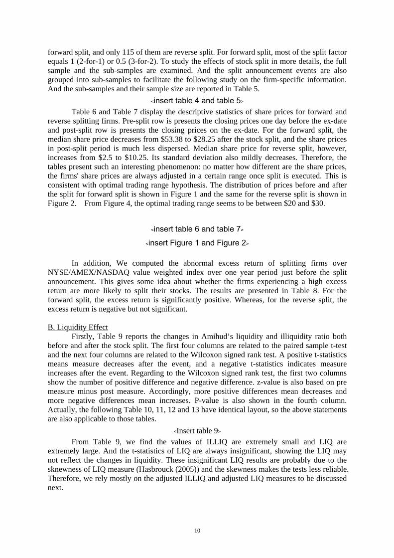
﹤insert table 4 and table 5﹥ Table 6 and Table 7 display the descriptive statistics of share prices for forward and

reverse splitting firms. Pre-split row is presents the closing prices one day before the ex-date and post-split row is presents the closing prices on the ex-date. For the forward split, the median share price decreases from $53.38 to $28.25 after the stock split, and the share prices in post-split period is much less dispersed. Median share price for reverse split, however, increases from $2.5 to $10.25. Its standard deviation also mildly decreases. Therefore, the tables present such an interesting phenomenon: no matter how different are the share prices, the firms' share prices are always adjusted in a certain range once split is executed. This is consistent with optimal trading range hypothesis. The distribution of prices before and after the split for forward split is shown in Figure 1 and the same for the reverse split is shown in Figure 2. From Figure 4, the optimal trading range seems to be between $20 and $30.

﹤insert table 6 and table 7﹥

﹤insert Figure 1 and Figure 2﹥

In addition, We computed the abnormal excess return of splitting firms over NYSE/AMEX/NASDAQ value weighted index over one year period just before the split announcement. This gives some idea about whether the firms experiencing a high excess return are more likely to split their stocks. The results are presented in Table 8. For the forward split, the excess return is significantly positive. Whereas, for the reverse split, the excess return is negative but not significant. B. Liquidity Effect

Firstly, Table 9 reports the changes in Amihud’s liquidity and illiquidity ratio both before and after the stock split. The first four columns are related to the paired sample t-test and the next four columns are related to the Wilcoxon signed rank test. A positive t-statistics means measure decreases after the event, and a negative t-statistics indicates measure increases after the event. Regarding to the Wilcoxon signed rank test, the first two columns show the number of positive difference and negative difference. z-value is also based on pre measure minus post measure. Accordingly, more positive differences mean decreases and more negative differences mean increases. P-value is also shown in the fourth column. Actually, the following Table 10, 11, 12 and 13 have identical layout, so the above statements are also applicable to those tables.

﹤Insert table 9﹥ From Table 9, we find the values of ILLIQ are extremely small and LIQ are

extremely large. And the t-statistics of LIQ are always insignificant, showing the LIQ may not reflect the changes in liquidity. These insignificant LIQ results are probably due to the sknewness of LIQ measure (Hasbrouck (2005)) and the skewness makes the tests less reliable. Therefore, we rely mostly on the adjusted ILLIQ and adjusted LIQ measures to be discussed next.

10

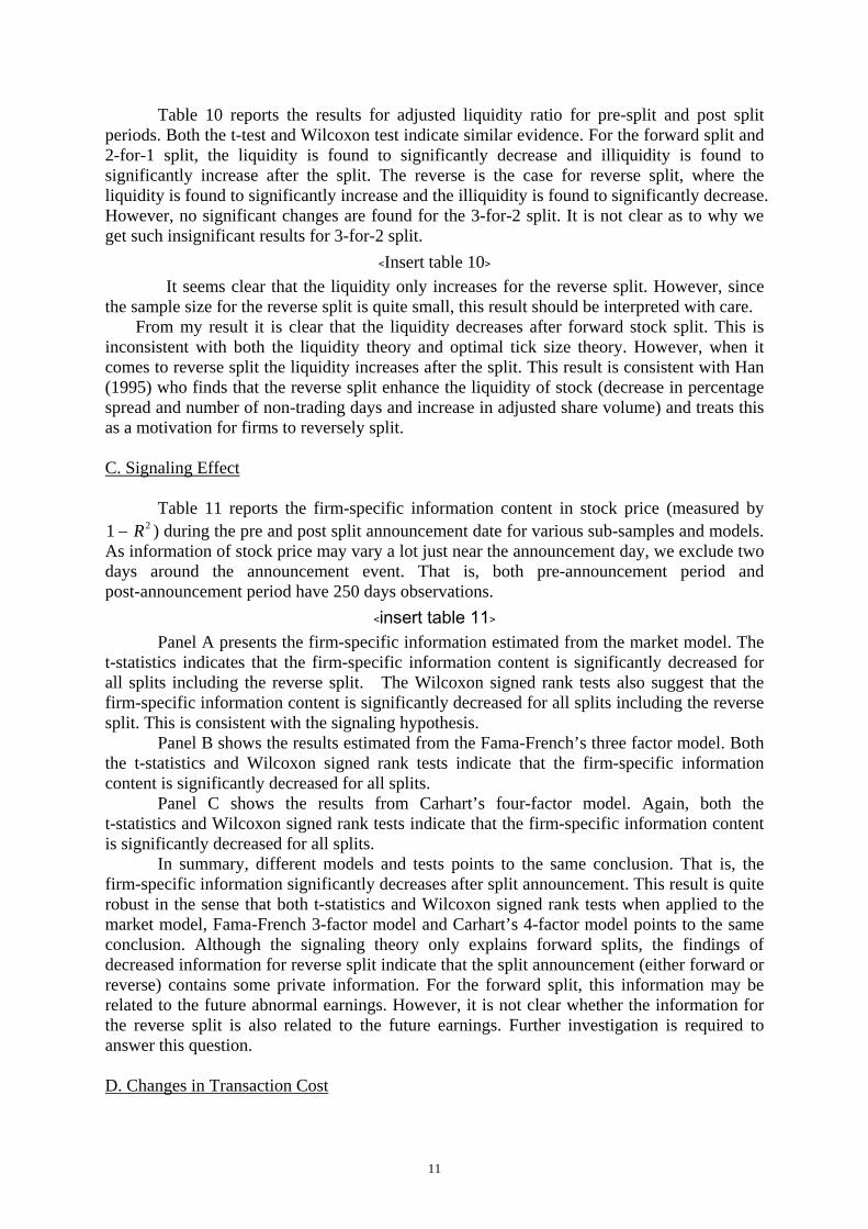
Table 10 reports the results for adjusted liquidity ratio for pre-split and post split periods. Both the t-test and Wilcoxon test indicate similar evidence. For the forward split and 2-for-1 split, the liquidity is found to significantly decrease and illiquidity is found to significantly increase after the split. The reverse is the case for reverse split, where the liquidity is found to significantly increase and the illiquidity is found to significantly decrease. However, no significant changes are found for the 3-for-2 split. It is not clear as to why we get such insignificant results for 3-for-2 split.

﹤Insert table 10﹥ It seems clear that the liquidity only increases for the reverse split. However, since the sample size for the reverse split is quite small, this result should be interpreted with care.

From my result it is clear that the liquidity decreases after forward stock split. This is inconsistent with both the liquidity theory and optimal tick size theory. However, when it comes to reverse split the liquidity increases after the split. This result is consistent with Han (1995) who finds that the reverse split enhance the liquidity of stock (decrease in percentage spread and number of non-trading days and increase in adjusted share volume) and treats this as a motivation for firms to reversely split. C. Signaling Effect

Table 11 reports the firm-specific information content in stock price (measured by 21 R− ) during the pre and post split announcement date for various sub-samples and models.

As information of stock price may vary a lot just near the announcement day, we exclude two days around the announcement event. That is, both pre-announcement period and post-announcement period have 250 days observations.

﹤insert table 11﹥ Panel A presents the firm-specific information estimated from the market model. The

t-statistics indicates that the firm-specific information content is significantly decreased for all splits including the reverse split. The Wilcoxon signed rank tests also suggest that the firm-specific information content is significantly decreased for all splits including the reverse split. This is consistent with the signaling hypothesis.

Panel B shows the results estimated from the Fama-French’s three factor model. Both the t-statistics and Wilcoxon signed rank tests indicate that the firm-specific information content is significantly decreased for all splits.

Panel C shows the results from Carhart’s four-factor model. Again, both the t-statistics and Wilcoxon signed rank tests indicate that the firm-specific information content is significantly decreased for all splits.

In summary, different models and tests points to the same conclusion. That is, the firm-specific information significantly decreases after split announcement. This result is quite robust in the sense that both t-statistics and Wilcoxon signed rank tests when applied to the market model, Fama-French 3-factor model and Carhart’s 4-factor model points to the same conclusion. Although the signaling theory only explains forward splits, the findings of decreased information for reverse split indicate that the split announcement (either forward or reverse) contains some private information. For the forward split, this information may be related to the future abnormal earnings. However, it is not clear whether the information for the reverse split is also related to the future earnings. Further investigation is required to answer this question. D. Changes in Transaction Cost

11

D.1 Gibbs Sampler Method

Table 12 reports the transaction cost estimated from Gibbs sampler method. As Table 9, the statistics are also based on pre-split measure minus post measure. The value in column 2 and column 3 is the cross-sectional average transaction cost.

﹤Insert table 12﹥ For forward split, mean transaction cost is found to significantly increases with

t-statistic equal to -36.11. The same is true for the 2-for-1 and 3-for-2 sub-samples. When it comes to the reverse split sub-sample, the transaction cost is found to significantly decreases with t-statistics equal to 12.13.

Similar result is obtained using the Wilcoxon sign rank tests, i.e., the transaction cost increases for forward split and decreases for reverse split. D.2 LDV Method

Table 13 reports the transaction cost estimated from LDV model. The results with the market model are presented in Panel A and the results with extended Lesmond’s method are presented in Panel B.

﹤Insert table 13﹥ For forward split, the mean transaction cost is found to significantly increase with the

t-statistics equal to -27.04. For 2-for-1 and 3-for-2 sub-samples, as the main components of forward splits, the round-trip transaction costs have been found to significantly increase. Whereas, for the reverse split, the transaction cost is found to significantly decreases with t-statistics equal to 9.78.

When the changes of transaction cost are further tested with Wilcoxon sign rank test, similar results are obtained. Similar results are found based on the extended model given in Panel B.

In summary, the transaction costs are found to increase for the forward split and decrease for the reverse split. Furthermore, it is important to note that the results are highly significant.

In addition to the paired t-test and Wilcoxon signed rank test of LDV measures, we count the number of significant changes on firm basis.

﹤Insert table 14﹥ Firstly, t-statistic, based on roundtrip cost before the split minus that after the split,

has been calculated for each firm. Then, the number of significant t-statistics (at 5% significance level) is counted. The significant t-statistics can be positive or negative. A positive t-value means a decrease in the transaction cost and negative t-value indicates an increase in transaction cost after the split. From Panel A, it is clear that most of the changes are negative for forward split and positive for reverse split. The results from Fama-French model, shown in Panel B, are also similar in nature. In summary, the transaction cost for forward split is found to increase and the transaction cost for the reverse split is found to decrease.

we can summarize the results as it applies to the three theories discussed before as follows: Liquidity Theory: The results for the reverse split supports this theory in the sense that the reverse split is associated with the higher liquidity. However, when it comes to the forward split, the

12

liquidity is found to decrease instead of increase. Therefore, the liquidity theory is not supported by the results associated with forward split. Some researchers have considered transaction cost as part of liquidity measure in the sense that higher liquidity is associated with lower transaction cost. If we use this argument, then only the reverse split seems to support the liquidity theory because only for the reverse split the transaction cost has been found to decrease. But, this theory is not supported by the evidence regarding forward split where the transaction cost is found to increase after the stock split. Signaling Theory: Since the firm-specific information content in stock price has been found to decrease for both the forward as well as the reverse split during the post-split announcement period, the signaling theory is strongly supported by the evidence. Optimal Tick Size Theory: According to this theory, the transaction cost should increase and liquidity should also increase. The evidence regarding forward split indicates a significant increase in transaction cost but at the same time a significant decrease in liquidity. When it comes to the reverse split, the transaction cost is found to decrease and liquidity is found to significantly increase. Therefore, the evidence does not seem to support the optimal tick size theory. 4. SUMMARY AND CONCLUSION

In this dissertation, we investigate the consistency of three main theories of stock split with the empirical evidence. The three theories are liquidity theory, signaling theory and optimal tick size theory. In order to get a clearer picture regarding the impacts of stock splits, we use recently proposed methods as well as extend some existing methods.

We find that liquidity significantly decreases after forward stock splits and

significantly increases after reverse splits. This evidence of decreased liquidity for forward split is inconsistent with the Liquidity theory. However, the increased liquidity for the reverse split is consistent with the liquidity hypothesis.

As to the signaling theory, the firm-specific information content in a stock price is

measured by 1 minus R-squared in a regression using market model as well as extended market model. The results indicate that the firm-specific information content significantly decreases after the announcement of the stock split including reverse split. Thus, these results strongly support the signaling theory that split announcements convey managers’ private information to the public. For the forward split, this information may be related to the future abnormal earnings. However, it is not clear whether the information for the reverse split is also related to the future earnings. Further investigation is required to answer this question.

Finally, we also estimated the effect of split on the transaction cost. It is found that the

round-trip transaction cost significantly increases after forward split and significantly decreases after reverse split. This result is consistent regardless of the methods used. This shows the robustness of the result. Therefore, for the forward split, it is found that the transaction cost increases but the liquidity decreases. As to the reverse split, the liquidity increases but the transaction cost is found to decrease. Therefore, the optimal tick size theory, which predicts both the transaction cost as well as the liquidity to increase after the split, is not consistent with the empirical evidence.

13

In conclusion, liquidity theory is not supported except for the reverse split. The optimal tick size theory is also not supported for both the forward split and reverse split. Only the signaling theory is fully supported. However, what signal the reverse split conveys is unknown. Future research is required to answer this question.

It would be interesting to see if the similar result holds using high frequency data. We

would suggest this for the future research.

14

REFERENCES Angel, James J. (1997), Tick size, share prices, and stock splits, Journal of Finance, Vol. 52, No. 2, PP. 655-681 Amihud, Yakov (2002), Illiquidity and stock returns: cross-section and time-series effects, Journal of Financial Markets, Vol. 5, PP. 31-56 Amihud, Yakov & Haim Mendelson (1987), Trading mechanisms and stock returns: an empirical investigation, Journal of Finance, Vol. 42, 533-553 Asquith, P., P. Healy and K. Palepu (1989), Earnings and stock splits, The Accounting Review, 64, 3, 387-404 Baker, H. Kent and Patricia L. Gallagher (1980), Management’s view of stock splits, Financial Management, 9, 73-77 Bar-Yosef, Sasson, Lawrence D. Brown (1977), A reexamination of stock splits using moving betas, The Journal of Finance, Vol. 32, No. 4, PP. 1069-1080 Brennan, Michael. J., Thomas. E. Copeland (1988a), Stock splits, stock prices, and transaction costs, Journal of Financial Economics, Vol. 22, PP. 83-101 Brennan, Michael. J., Thomas. E. Copeland (1988b), Beta changes around stock splits: A note, Journal of Finance, Vol. 43, No. 4, 1009-1013 Carhart, Mark M. (1997), On persistence in mutual fund performance, Journal of Finance, Vol. 52, 57-82 Conrad, Jennifer S., Robert Conroy (1994), Market microstructure and the ex-date return, the Journal of Finance, Vol. 49, No. 4, PP. 1507-1519 Conroy, Robert M, Robert S. Harris (1999), Stock splits and information: the role of share price, Financial Management, Vol. 28, 28-40 (FM, 1999 event study- event date is take from CRSP – is this the announcement date). Copeland, Thomas E. (1979), Liquidity changes following stock splits, Journal of Finance, Vol. 34, No.1, PP. 115-141 Conroy, Robert M., Robert S. Harris, Bruce A. Benet (1990), The effects of stock splits on Bid-ask spreads, The Journal of Finance, Vol. 45, No. 4, PP. 1285-1295 Desai, Anand S., M. Nimalendran, S. Venkataraman (1998), Changes in trading activity following stock splits and their effect on volatility and the adverse-information component of the bid-ask spread, Journal of Financial Research, Vol. XXI, 159-183 Dravid, Ajay R. (1987), A note on the behavior of stock returns around Ex-dates of stock distributions, The Journal of Finance, Vol. 42, 163-168

15

Dubofsky, David A. (1991): volatility increases subsequent to NYSE and AMEX stock splits, Journal of Finance, Vol. 46, 421-431 Durnev, Art, Randall Morck, Bernard Yeung (2004), Value-enhancing capital budgeting and firm-specific stock return variation, The Journal of Finance, Vol. LIX, No. 1 Durnev, Art, Randall Morck, Bernard Yeung (2003), Does greater firm-specific return variation mean more or less informed stock pricing?, Journal of Accounting Research, Vol. 41, No. 5 Dennis, Patrick (2003), Stock splits and liquidity: the case of the Nasdaq-100 Index Tracking Stock, The Financial Review, Vol. 38, PP. 415-433 Dhar, Ravi, William N. Goetzmann, Shane Shepherd, Ning Zhu (2003), The impact of clientele changes: evidence from stock splits, working paper Easley, David, Maureen O’hara, Gideon Saar (2000), How stock splits affect trading: a microstructure approach, The Journal of Financial and Quantitative Analysis, Vol. 36, No. 1, PP. 25-51 French, DW, DA Dubofsky (1986), Stock splits and implied stock price volatility, Journal of Portfolio Management, French, Dan W., Taylor W. Foster (2002), Does price discreteness affect the increase in return volatility following stock splits?, The Financial Review, Vol. 37, 281-294 Fama, Eugene F., Lawrence Fisher, Michael C. Jensen, Richard Roll (1969), The adjustment of stock prices to new information, International Economic Review, Vol. 10, No. 1, PP. 1-21 French & Dubofsky (1986), Stock splits and implied stock price volatility, Journal of Portfolio Management, Vol.12, Iss. 4; pg. 55 GUIRAO JOSÉ YAGÜE, J. CARLOS GÓMEZ SALA (2002), Transaction size, order submission and price preference around stock splits, working paper Goyenko Ruslan, Craig W. Holden, Christian T. Lundblad, Charles A. Trzcinka (2005a), Horseraces of monthly and annual liquidity measures, working paper from Indiana University Goyenko Ruslan Y., Craig W. Holden, Andrey D. Ukhov (2005b), Do stock splits improve liquidity?, working paper from Indiana University Grinblatt Mark S., Ronald W. Masulis, Sheridan Titman (1984): the valuation effects of stock splits and stock dividends, Journal of Finanacial Economics, Vol. 13, PP. 461-490 Han Ki C. (1995), The effects of reverse split on the liquidity of the stock, Journal of Financial and Quantitative Analysis, 30, 159-169 Hasbrouck Joel (2004), Liquidity in the futures pits: Inferring Market Dynamics from incomplete data, Journal of Financial and Quantitative Analysis, Vol. 39, No. 2

16

Hasbrouck Joel (2003), Trading costs and returns for US equities: the evidence from daily data, working paper Huson Mark R., Gregory MacKinnon (2003), Corporate spinoffs and information asymmetry between investors, Journal of Corporate Finance, Vol. 9, PP 481-503 Ikenberry David L., Graeme Rankine, Earl K. Stice (1996), What do stock splits really singal?, The Journal of Financial and Quantitative Analysis, Vol. 31, No. 3, PP. 357-375 Klein L.S, and D.R. Peterson, 1989, Earnings Forecast Revisions Associated with Stock Split Announcements, Journal of Financial Research 12, No. 4, pp. 319-328. Koski Jennifer Lynch (1998), Measurement effects and the variance of returns after stock splits and stock dividends, the review of financial studies, Vol. 11, 143-162 Lakonishok Josef, Baruch Lev (1987), Stock splits and stock dividends: why, who and when, Journal of Finance, Vol. 42, 913-932 Lamoureux Christopher G., Percy Poon (1987), The market reaction to stock splits, Journal of Finance, Vol. 42, 1347-1370 Lesmond David A., Joseph P. Ogden, Charles A. Trzcinka (1999), A new estimate of transaction costs, Review of Financial Studies, Vol. 12, No. 5, PP. 1113-1141 Lipson Marc L. (1999), Stock splits, liquidity and limit orders, working paper Murray, Dennis (1985), Further Evidence on the Liquidity Effects of Stock Splits and Stock Dividends, The Journal of Financial Research, Vol. 8, Iss. 1; p. 59-68 Muscarella Chris J., Michael R. Vetsuypens (1996), Stock splits: signaling or liquidity? The case of ADR ‘solo-splits’, Journal of Financial Economics, Vol. 42, 3-26 Ohlson James A., Stephen H. Penman (1985), Volatility increases subsequent to stock splits, Journal of Financial Economics, Vol. 14, 251-266 Pastor Lubos, Robert F. Stambaugh (2003), Liquidity risk and expected stock returns, Journal of Political Economy, Vol. 111, No. 3 Roll, R. (1984), A Simple Implicit Measure of the Effective Bid-Ask Spread in an Efficient Market, Journal of Finance, 39, 1127-1139. Roll Richard (1988), R2, Journal of Finance, Vol. 43, No. 3, PP 541-566 Sheikh Aamir M. (1989), Stock splits, volatility increases, and implied volatilities, The Journal of Finance, Vol. 44, No. 5, PP. 1361-1372 Schultz Paul (2000), Stock splits, tick size, and sponsorship, The Journal of Finance, Vol. LV, No. 1

17

Woolridge Randall J., Donald R. Chambers (1983), Reverse splits and shareholders wealth, Financial Management, Vol. 12, No. 3 Wulff Christian (2002), The market reaction to stock splits-evidence from Germany, Schmalenbach Business Review, V54, 270-297 Wiggins James B. (1992), Beta changes around stock splits revisited, The Journal of Financial and Quantitative Analysis, Vol. 27, No. 4, PP. 631-640

18

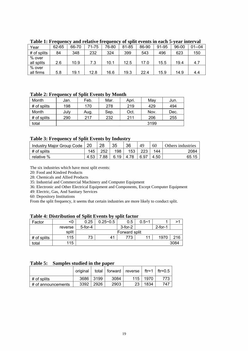
Table 1: Frequency and relative frequency of split events in each 5-year interval Year 62-65 66-70 71-75 76-80 81-85 86-90 91-95 96-00 01--04 # of splits 84 348 232 324 399 543 496 623 150 % over all splits 2.6 10.9 7.3 10.1 12.5 17.0 15.5 19.4 4.7 % over all firms 5.8 19.1 12.8 16.6 19.3 22.4 15.9 14.9 4.4 Table 2: Frequency of Split Events by Month Month Jan. Feb. Mar. Apri. May Jun. # of splits 198 170 278 219 429 494 Month July Aug. Sep. Oct. Nov. Dec. # of splits 290 217 232 211 206 255 total 3199

Table 3: Frequency of Split Events by Industry Industry Major Group Code 20 28 35 36 49 60 Others industries # of splits 145 252 198 153 223 144 2084 relative % 4.53 7.88 6.19 4.78 6.97 4.50 65.15

The six industries which have most split events: 20: Food and Kindred Products 28: Chemicals and Allied Products 35: Industrial and Commercial Machinery and Computer Equipment 36: Electronic and Other Electrical Equipment and Components, Except Computer Equipment 49: Electric, Gas, And Sanitary Services 60: Depository Institutions From the split frequency, it seems that certain industries are more likely to conduct split. Table 4: Distribution of Split Events by split factor Factor <0 0.25 0.25~0.5 0.5 0.5~1 1 >1

5-for-4 3-for-2 2-for-1

reverse split Forward split

# of splits 115 73 41 773 11 1970 216 total 115 3084

Table 5: Samples studied in the paper original total forward reverse ftr=1 ftr=0.5

# of splits 3686 3199 3084 115 1970 773# of announcements 3392 2926 2903 23 1834 747

19

Table 6: Descriptive statistics of stock prices for forward split Minimum 25% Median 75% Maximum Mean std. dev. Pre-split 3.06 39.38 53.25 74.25 1370 60.85 41.83 Post-split 2.38 22.13 28.25 37.25 138 30.93 13.19

10 splits did not trade just before the split date and 3 splits which did not trade on the split date, so the prices on that non-trading day is shown as negative. The prices of these events are set as positive value of the negative price on that day (this is justified by the notation of CRSP data). Table 7: Descriptive statistics of stock prices for reverse split

Minimum 25% Median 75% Maximum Mean std dev. Pre-split 0.09 1 2.5 3.94 93.44 4.9 10.19

Post-split 1.13 6.59 10.25 17.7 38.75 12.65 8.17 Table 8: Abnormal return of forward splits over NYSE/AMEX/NASDAQ value weighted index measured in one-year period just before the split announcement

mean excess return sample size t value

forward 0.3596 2903 28.476 reverse -0.1008 23 -0.593

20

21

Figure 1:

Figure 2:

0

50

100

150

200

250

300

frequency

0 5 10 15 20 25 30 35 40 45 50 55 60 65 70 75 80 85 90 95 100105110115120125130More

price just before the ex-date

Frequency of Stock Prices just Before the Forward Split

0100200300400500600700

frequency

0 5 10 15 20 25 30 35 40 45 50 55 60 65 70 75 80 85 90 95 100105110115120125130More

price on the ex-date

Frequency of Stock Prices just After the Forward Split

0

510

1520

2530

35

0 1 2 3 4 5 6 7 8 9 10 11 12 13 14 15More

Frequency of Stock Prices just Before the Reverse Split

05

1015202530354045

0 1 2 3 4 5 6 7 8 9 10 11 12 13 14 15More

Frequency of Stock Prices just After the Reverse Split

Table 9: Changes in the liquidity (measured by ILLIQ and LIQ) after the stock split

Paired Sample t-test for Mean Wilcoxon Signed Rank Test for Median

Average Pre-Split

Average Post-Split

t-statistc Pre Minus Post p-value positive d negative d z-statistc

p-value (2-tailed)

ILLIQ total 1.91E-07 1.54E-07 1.10 0.14 1510 1678 -2.35 0.02forward split 9.64E-08 1.11E-07 -3.24 0.00 1428 1646 -3.89 0.00reverse split 2.73E-06 1.30E-06 1.53 0.06 82 32 4.67 0.00ftr=1 7.69E-08 1.02E-07 -4.36 0.00 863 1103 -6.19 0.00ftr=0.5 1.44E-07 1.36E-07 0.98 0.16 426 343 2.25 0.02 LIQ total 1.46E9 1.41E9 1.21 0.11 1925 1268 10.46 0.00forward split 1.51E9 1.45E9 1.21 0.11 1901 1177 11.22 0.00reverse split 3.29E8 3.27E8 0.04 0.48 24 91 -5.15 0.00ftr=1 1.67E9 1.67E9 -0.09 0.46 1282 684 10.68 0.00ftr=0.5 6.35E8 6.53E8 -0.30 0.38 394 377 -0.36 0.72

0,11

>= ∑=

t

T

t t

t VolVolR

TILLIQ

0,11

≠= ∑=

t

T

t t

t RR

VolT

LIQ

Both t-test and Wilcoxon signed rank test are based on the measure before split minus that after split.

22

Table 10: Changes in the liquidity (measured by adjusted ILLIQ and LIQ) after the stock split

Paired Sample t-test for Mean Wilcoxon Signed Rank Test for Median

Adjusted Average Pre-Split

Average Post-Split

t-statistic Pre Minus Post p-value

positive d

negative d z-statistic

p-value (2-tailed)

Panel A: ILLIQ total 1.90E-4 1.92E-4 -1.09 0.14 1493 1690 -3.10 0.00forward split 1.73E-4 1.81E-4 -5.08 0.00 1412 1656 -4.50 0.00reverse split 6.34E-4 4.85E-4 2.75 0.00 81 34 4.35 0.00ftr=1 1.56E-4 1.69E-4 -6.63 0.00 854 1106 -6.63 0.00ftr=0.5 2.17E-4 2.14E-4 0.86 0.19 415 354 1.85 0.06 Panel B: LIQ total 1.93E4 1.87E4 4.69 0.00 1868 1331 8.95 0.00forward split 1.98E4 1.92E4 5.20 0.00 1842 1242 10.14 0.00reverse split 6.02E3 7.38E3 -2.33 0.01 26 89 -5.43 0.00ftr=1 2.19E4 2.13E4 4.14 0.00 1239 731 10.10 0.00ftr=0.5 1.24E4 1.27E4 -1.34 0.09 383 390 -1.07 0.28

0,11

>= ∑=

t

T

t t

t VolVolR

TILLIQ

0,11

≠= ∑=

t

T

t t

t RR

VolT

LIQ

Both t-test and Wilcoxon signed rank test are based on the measure before split minus that after split.

23

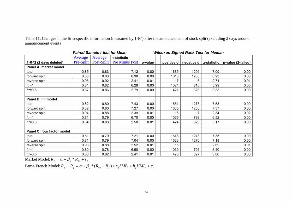
Table 11: Changes in the firm-specific information (measured by 1-R2) after the announcement of stock split (excluding 2 days around announcement event) Paired Sample t-test for Mean Wilcoxon Signed Rank Test for Median

1-R^2 (2 days deleted) Average Pre-Split

Average Post-Split

t-statistic Pre Minus Post p-value positive d negative d z-statistic p-value (2-tailed)

Panel A: market model total 0.85 0.83 7.12 0.00 1635 1291 7.09 0.00forward split 0.85 0.83 6.98 0.00 1618 1285 6.93 0.00reverse split 0.96 0.92 2.41 0.01 17 6 2.71 0.01ftr=1 0.84 0.82 6.29 0.00 1024 810 5.99 0.00ftr=0.5 0.87 0.86 2.79 0.00 421 326 3.33 0.00 Panel B: FF model total 0.82 0.80 7.43 0.00 1651 1275 7.53 0.00forward split 0.82 0.80 7.27 0.00 1635 1268 7.37 0.00reverse split 0.94 0.88 2.39 0.01 16 7 2.34 0.02ftr=1 0.81 0.79 6.70 0.00 1035 799 6.52 0.00ftr=0.5 0.84 0.83 2.50 0.01 424 323 3.17 0.00 Panel C: four factor model total 0.81 0.79 7.21 0.00 1648 1278 7.35 0.00forward split 0.81 0.79 7.04 0.00 1633 1270 7.18 0.00reverse split 0.93 0.88 2.52 0.01 15 8 2.62 0.01ftr=1 0.80 0.78 6.50 0.00 1039 795 6.40 0.00ftr=0.5 0.83 0.82 2.41 0.01 420 327 3.00 0.00

Market Model: tmtjjt RR εβα +*= + Fama-French Model: ttjtjfmtjfjt HMLhSMBsRRRR εβα +++−+=− )(*

24

Four Factor Model: ttjtjtjfmtjfjt YRPRmHMLhSMBsRRRR εβα ++++−+=− 1)(* Both tests are based on the firm-specific information before the announcement minus that after the announcement. Table 12: Changes in the transaction cost (measured from Gibbs sampler method) after stock split

Paired Sample t-test for Mean Wilcoxon Signed Rank Test for Median

Average Pre-Split

Average Post-Split

t-statistic Pre Minus Post p-value positive d negative d z-statistic

p-value (2-tailed)

Gibbs sampler total 3.69E-3 4.41E-3 -8.81 0.00 683 2516 -30.53 0.00forward split 2.87E-3 4.22E-3 -36.11 0.00 580 2504 -34.81 0.00reverse split 2.57E-2 9.70E-3 12.13 0.00 103 12 8.57 0.00ftr=1 2.56E-3 4.16E-3 -36.53 0.00 275 1695 -31.77 0.00ftr=0.5 3.59E-3 4.27E-3 -8.65 0.00 232 541 -10.80 0.00

Both t-test and Wilcoxon signed rank test are based on the transaction cost before split minus that after split.

25

26

Table 13: Changes in the transaction cost (measured by α2-α1) after stock split

Paired Sample t-test for Mean Wilcoxon Signed Rank Test for Median

Average Pre-Split

Average Post-Split

t-statistic Pre Minus Post p-value positive d negative d z-statistic

p-value (2-tailed)

α2-α1 Panel A: market model total 8.76E-3 8.65E-3 0.39 0.35 878 2288 -25.17 0.00forward split 5.78E-3 7.69E-3 -27.04 0.00 778 2273 -29.09 0.00reverse split 8.78E-2 3.40E-2 9.78 0.00 100 15 8.42 0.00ftr=1 4.95E-3 7.10E-3 -27.76 0.00 411 1534 -27.42 0.00ftr=0.5 7.78E-3 9.00E-3 -6.93 0.00 293 476 -7.63 0.00 Panel B: FF model total 8.74E-3 8.61E-3 0.46 0.32 881 2280 -25.14 0.00forward split 5.75E-3 7.65E-3 -26.98 0.00 781 2265 -29.06 0.00reverse split 8.76E-2 3.39E-2 9.79 0.00 100 15 8.42 0.00ftr=1 4.93E-3 7.07E-3 -27.58 0.00 411 1533 -27.36 0.00ftr=0.5 7.74E-3 8.95E-3 -6.96 0.00 298 469 -7.64 0.00

Market Model:

Both t-test and Wilcoxon signed rank test are based on the transaction cost before split minus that after split.

Fama-French Model: ttjtjfmtjfjt HMLhSMBsRRRR εβα +++−+=− )(* tmtjjtR εRβα ++= *

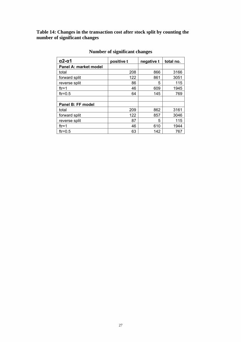
Table 14: Changes in the transaction cost after stock split by counting the number of significant changes

Number of significant changes

α2-α1 positive t negative t total no. Panel A: market model total 208 866 3166 forward split 122 861 3051 reverse split 86 5 115 ftr=1 46 609 1945 ftr=0.5 64 145 769 Panel B: FF model total 209 862 3161 forward split 122 857 3046 reverse split 87 5 115 ftr=1 46 610 1944 ftr=0.5 63 142 767

27

28