A New Method of Estimating Risk Aversion - Raj · PDF fileA New Method of Estimating Risk...
26
A New Method of Estimating Risk Aversion Raj Chetty Abstract This paper develops a new method of estimating risk aversion using data on labor supply behavior. In particular, I show that existing evidence on labor supply behavior places a tight upper bound on risk aversion in the expected utility model. I derive a formula for the coe¢ cient of relative risk aversion ( ) in terms of (1) the ratio of the income elasticity of labor supply to the wage elasticity and (2) the degree of complementarity between consumption and labor. I bound the degree of complementarity using data on consumption choices when labor supply varies randomly across states. Using labor supply elasticity estimates from thirty-three studies, I nd a mean estimate of 1: I then show that generating > 2 would require that wage increases cause sharper reductions in labor supply than estimated in any of the studies. (JEL D80, J20, J60) Department of Economics, University of California, Berkeley and NBER, 549 Evans Hall #3880, Berkeley CA 94709 USA (email: [email protected]). This paper is based on the second chapter of my Ph.D. thesis at Harvard. I thank George Akerlof, John Campbell, David Card, Gary Chamberlain, David Cutler, Martin Feldstein, John Friedman, Ed Glaeser, Caroline Hoxby, Louis Kaplow, Larry Katz, Miles Kimball, Greg Mankiw, Richard Rogerson, anonymous referees, and numerous seminar participants for very helpful comments and discussions. Financial support from the National Science Foundation Graduate Fellowship, the National Bureau of Economic Research, and Harvard University is gratefully acknowledged. 1
Transcript of A New Method of Estimating Risk Aversion - Raj · PDF fileA New Method of Estimating Risk...

A New Method of Estimating Risk Aversion
Raj Chetty�
Abstract
This paper develops a new method of estimating risk aversion using data on laborsupply behavior. In particular, I show that existing evidence on labor supplybehavior places a tight upper bound on risk aversion in the expected utilitymodel. I derive a formula for the coe¢ cient of relative risk aversion ( ) in termsof (1) the ratio of the income elasticity of labor supply to the wage elasticity and(2) the degree of complementarity between consumption and labor. I boundthe degree of complementarity using data on consumption choices when laborsupply varies randomly across states. Using labor supply elasticity estimatesfrom thirty-three studies, I �nd a mean estimate of � 1: I then show thatgenerating > 2 would require that wage increases cause sharper reductions inlabor supply than estimated in any of the studies. (JEL D80, J20, J60)
�Department of Economics, University of California, Berkeley and NBER, 549 Evans Hall #3880, BerkeleyCA 94709 USA (email: [email protected]). This paper is based on the second chapter of my Ph.D.thesis at Harvard. I thank George Akerlof, John Campbell, David Card, Gary Chamberlain, David Cutler,Martin Feldstein, John Friedman, Ed Glaeser, Caroline Hoxby, Louis Kaplow, Larry Katz, Miles Kimball,Greg Mankiw, Richard Rogerson, anonymous referees, and numerous seminar participants for very helpfulcomments and discussions. Financial support from the National Science Foundation Graduate Fellowship,the National Bureau of Economic Research, and Harvard University is gratefully acknowledged.
1

Expected utility is the canonical theory of choice under uncertainty in economics. In
the expected utility model, risk aversion arises from the curvature of the utility function,
typically measured by the coe¢ cient of relative risk aversion ( ). Despite its importance in
many microeconomic and macroeconomic models, the value of remains disputed, largely
because of limitations in estimating risk aversion empirically.
This paper develops a new method of estimating using data on labor supply behavior.
In particular, I show that existing evidence on the e¤ects of wage changes on labor supply
imposes a tight upper bound on the curvature of utility over wealth ( < 2). Hence,
the standard expected utility model cannot generate high levels of risk aversion without
contradicting established facts about labor supply.
Labor supply behavior and risk aversion are tightly linked in the expected utility model
because both are determined by the curvature of utility over consumption. To see the
connection, consider the e¤ect of a wage increase on labor supply in a static model where an
agent maximizes utility over consumption and leisure. If the marginal utility of consumption
diminishes quickly, the individual becomes sated with goods as wages rise. A highly risk
averse individual will therefore choose to consume more leisure (by reducing labor supply)
as wages rise. More generally, a higher curvature of utility over consumption implies a lower
uncompensated wage elasticity of labor supply.
The bound on risk aversion is obtained by combining this logic with empirical evidence
on the wage elasticity. A well established �nding of the labor supply literature is that wage
increases do not cause sharp reductions in labor supply. This lower bound on the wage
elasticity of labor supply places an upper bound on the curvature of utility over consumption
and hence on risk aversion. The fact that individuals do not choose to reduce labor supply
sharply when wages rise implies that their marginal utility of consumption does not diminish
quickly, unless consumption and labor are very complementary.
If complementarity between consumption and labor is su¢ ciently strong, even highly
risk averse individuals may choose not to reduce labor supply when wages rise because
increased consumption makes work less painful. Therefore, bounding using labor supply
elasticities requires that we �rst bound the degree of complementarity between consumption
and labor. Such a bound can be obtained from evidence on consumption choices when agents
1
face uncertainty about labor supply. Intuitively, the extent to which an agent chooses to
correlate consumption with labor across states where labor supply varies exogenously (e.g.,
because of job loss or disability) reveals the degree of complementarity. Combining the
bound on complementarity with estimates of labor supply elasticities yields a bound on
that does not rely on any assumptions beyond those inherent in expected utility theory.
I formalize the preceding logic in a dynamic lifecycle model with arbitrary non-separable
utility over consumption and leisure. I derive a formula for in terms of the ratio of the
income elasticity of labor supply to the substitution elasticity of labor supply along with the
cardinal complementarity parameter. I bound the complementarity parameter using a set
of estimates of the consumption drop associated with job loss and other exogenous shocks to
labor supply. I then estimate using labor supply elasticity estimates from various types of
microeconomic studies �e.g., structural lifecycle methods, natural experiments, and earned
income responses �as well as macroeconomic observations such as the downward trend in
labor supply over the past century. Using thirty-three sets of estimates of wage and income
elasticities, the mean implied value of is 0:71, with a range of 0:15 to 1:78 in the additive
utility case. At the upper bound for complementarity, the mean value of rises modestly,
to 0:97.
I clarify why all the labor supply studies imply a low level of despite disagreement about
the magnitudes of the elasticities using a calibration argument. I show that generating > 2
with a plausible level of complementarity requires an uncompensated wage elasticity of labor
supply more negative than that estimated in any of the thirty-three studies.
The bound on risk aversion derived here contrasts with the much higher estimates of
risk aversion obtained in studies of asset and insurance markets (e.g., Rajnish Mehra and
Edward Prescott 1985, Narayana Kocherlakota 1996, Robert Barsky et. al. 1997, Alma
Cohen and Liran Einav 2005, Justin Sydnor 2005). Hence, one interpretation of the result
is that it provides new evidence against the canonical expected utility theory as a descriptive
model of choice under uncertainty. Importantly, the calibration argument here restricts risk
preferences over all risks, and not just the small gambles or low probability events that are
the basis of many existing critiques (Chris Starmer 2000).
The paper proceeds as follows. Section I gives graphical intuition for the bounding
2

argument, and derives a formula for risk aversion in terms of labor supply elasticities and
complementarity between consumption and labor. Section II implements the formula using
existing estimates of these parameters. Section III discusses how this paper is related to
other recent calibration arguments for risk aversion and intertemporal substitution. Section
IV concludes.
I Theory
Setup. Consider a T period life-cycle model. Denote consumption in each period by ct and
labor supply by lt. Let U(c1; :::; cT ; l1; :::; lT ) denote utility over the consumption and labor
streams. Let pt denote the price of consumption in period t. Assume that U is smooth
and that Uct > 0; Ult < 0; uctct < 0; ultlt < 0. Let w�t denote the wage in period t and y
unearned income (wealth) at time 0. In Thomas MaCurdy�s (1981) terminology, a change
in �t is a transitory wage change, while changes in w are permanent wage changes, i.e. shifts
in the entire pro�le of wages over a lifetime.
The agent chooses a path of consumption and labor by solving
maxct;lt
U(c1; :::; cT ; l1; :::; lT )
s.t. p1c1 + :::+ pT cT = y + w(�1l1 + :::+ �T lT )
It is convenient to rewrite this problem as a two-stage maximization:
maxc;l
u(c; l) s.t. c = y + wl (1)
where u(c; l) = maxct;lt
U(c1; :::; cT ; l1; :::; lT )
s.t. p1c1 + :::+ pT cT = c
�1l1 + :::+ �T lT = l
In (1), c and l represent aggregates that capture total consumption and labor supply over
the lifecycle. The function u(c; l) is indirect utility over these two composite commodities.
Our goal is to derive a bound for the coe¢ cient of relative risk aversion of the indirect utility
3

function u(c; l), de�ned as follows:
(c; l) � �"uc;c =@uc(c; l)
@c
c
uc(c; l)= �ucc(c; l)
uc(c; l)c (2)
Note that is the curvature of utility over wealth � the parameter that determines risk
preferences over immediately-resolved wealth gambles in an expected utility model �when
total labor supply l is �xed. When l is variable, the curvature of utility over wealth is
strictly lower than (see appendix A for a proof). Intuitively, if the agent can adjust labor
supply, he has more �exibility to adjust to wealth shocks, and is less risk averse (Zvi Bodie
et. al. 1992). A bound on therefore bounds risk aversion when l is endogenous as well.
Bounding Risk Aversion: Graphical Example. The main result follows from the compar-
ative statics implied by the agent�s �rst order condition for l. At an interior optimum, the
marginal bene�t of working an extra hour equals the marginal cost:
wuc(y + wl; l) = �ul(y + wl; l) (3)
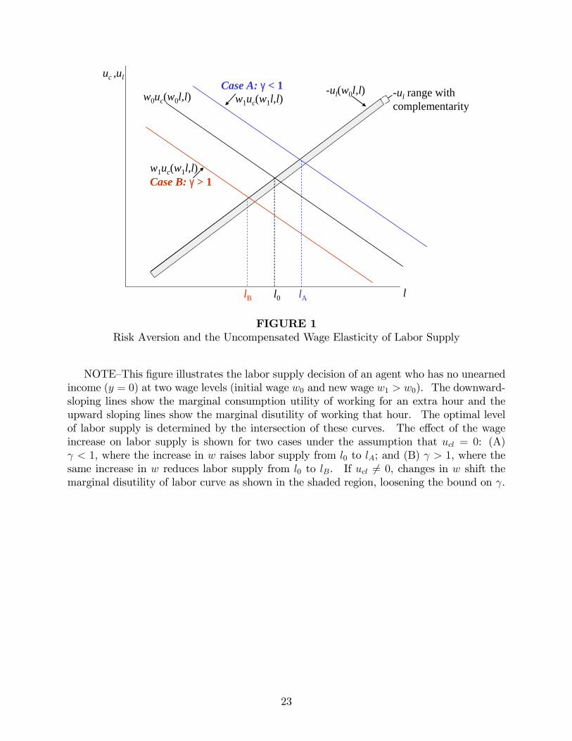
Figure 1 illustrates the calibration argument using this �rst order condition. It plots
the marginal consumption utility of working an extra hour, wuc(y +wl; l) and the marginal
disutility of working that hour, �ul(y + wl; l). The initial level of labor supply, l0, is
determined by the intersection of these two curves at the initial wage w0. For simplicity,
the �gure is drawn for a case where the agent has no unearned income (y = 0).
Suppose �rst that the agent has additive utility over c and l (ucl = 0). Consider the
e¤ect of raising w by 1 percent on l. This change has two e¤ects on the wuc curve, which
correspond to a substitution and income e¤ect on labor supply. The substitution e¤ect
is that the number multiplying uc rises by 1 percent, shifting the wuc curve upward by 1
percent. The 1 percent increase in w also increases consumption (wl) at any given level of
l by 1 percent. A 1 percent increase in consumption lowers uc by "uc;c = , so the 1 percent
wage increase shifts the wuc curve downward by percent via the income e¤ect. The total
shift in the wuc curve is thus (1� ) percent. This expression shows that higher makes the
wage elasticity of labor supply more negative by magnifying the income e¤ect. Intuitively,
when is high, the marginal bene�t of consumption falls quickly as the wage rises. This
4

strengthens the incentive to consume more leisure (by reducing l) when w rises.
Since changes in w do not a¤ect the �ul curve when ucl = 0, it follows that
@l=@w > 0, < 1
when y = 0. This result is the simplest version of the bound on risk aversion imposed
by labor supply behavior. The remainder of the paper generalizes this bound to allow for
positive unearned income (y > 0), a potentially negative wage elasticity of labor supply, and
complementarity between c and l. These factors loosen the bound on slightly (to < 2),
but the basic logic of the calibration argument is the same: If upward shifts in the wage
pro�le do not cause sharp reductions in lifetime labor supply, must be small.
Complementarity between c and l causes shifts in the �ul curve in Figure 1 as w rises. If
ucl > 0, the �ul curve shifts outward when w rises and l rises more than it would if ucl = 0.
Consequently, the value of estimated from labor supply elasticities under the assumption
that ucl = 0 understates the true if ucl > 0. This issue is addressed below using empirical
evidence from studies of consumption smoothing to place bounds on the magnitude of ucl.
Given these bounds, the range of possible shifts in the �ul curve is narrow, as illustrated by
the shaded region in Figure 1. The bound on is thus loosened modestly when plausible
levels of complementarity are permitted.
An Estimator for . To generalize the example in Figure 1, I derive a formula for in
terms of labor supply elasticities. Implicitly di¤erentiate (3) to obtain:
@l
@y= � wucc + ucl
w2ucc + ull + 2wucl(4)
@l
@w= � uc + wlucc + lucl
w2ucc + ull + 2wucl
Using the Slutsky decomposition for compensated labor supply (@lc
@w)
@lc
@w=@l
@w� l @l@y
(5)
5

it follows that the ratio of the income e¤ect to the substitution e¤ect is given by
@l=@y
@lc=@w=wucc + ucl
uc(6)
Let "l;y = @l@yyldenote the income elasticity of labor supply, "cl;w =
@lc
@wwlthe compensated wage
elasticity of labor supply, and "uc;l =uclucl the elasticity of the marginal utility of consumption
with respect to labor. Some algebraic rearrangement gives
= �y + wlw
@l=@y
@lc=@w+y + wl
w
ucluc= �(1 + wl
y)"l;y"lc;w
(y; w) + (1 +y
wl)"uc;l. (7)
This equation shows that is determined by the ratio of the income elasticity of labor
supply to the substitution elasticity of labor supply, with an adjustment for complementarity
between c and l.1 This is because the income e¤ect is proportional to ucc (how much the
marginal consumption utility from working falls when y is raised) while the substitution
e¤ect is proportional to uc (how much the marginal consumption utility from working rises
when w is raised). For example, when utility is linear in c, there are no income e¤ects in
labor supply, and = 0. Note that the formula for in (7) does not rely on any functional
form assumptions; hence, the bounds derived below apply to any utility function.
Cardinality and Complementarity. It may be surprising that a unique value for can be
identi�ed from labor-leisure choices. Since non-linear monotonic transformations of u(c; l)
do not a¤ect the choice of l, are there not in�nitely many values of that could be associated
with a given set of labor supply data? The reason that is identi�ed in (7) is that any
non-linear transformation of u would change the value of "uc;l. For example, non-linear
transformations of an additive u (with ucl = 0) destroy additivity. Labor supply data are
thus su¢ cient to identify conditional on the value "uc;l, which pins down the cardinal
normalization of u.
Since the cardinal complementarity parameter "uc;l is unknown, it must be estimated
from choices under uncertainty. A natural method of estimating "uc;l is to examine the
1Note that (7) remains well de�ned when y = 0. In that case, the �rst term in (7) equals �@lw@y ="lc;w.
The @lw@y term is the propensity to earn out of unearned income (in dollars rather than a percentage, which
would be unde�ned).
6

consumption choices of individuals who face exogenous variation in labor supply across states,
e.g. due to a shock such as job displacement. Intuitively, if agents choose to consume a
lot more in states where labor supply is high, c and l must be highly complementary; if in
contrast labor supply �uctuations are not correlated with consumption changes, c and l must
not be very complementary.
To obtain an estimate of "uc;l based on this logic, consider a setting with two states where
agents work for l1 hours in state 1 (which occurs with probability p) and l2 hours in state 2
(probability 1� p). Assume that preferences are state-independent, i.e. the utility function
in the two states is the same. Let ws denote the wage in state s. Suppose the agent
can trade consumption at an actuarially fair rate between the two states using an insurance
policy. We will see below that if perfect insurance of this form is unavailable, the exercise
below provides an upper bound for "uc;l and thereby an upper bound for .
Conditional on (l1; l2), the agent chooses a consumption allocation (c1; c2) to maximize
expected utility:
maxc1;c2
pu(c1; l1) + (1� p)u(c2; l2)
s.t. pc1 + (1� p)c2 = pw1l1 + (1� p)w2l2
At the optimal (c1; c2), marginal utilities are equated across the states:
uc(c1; l1) = uc(c
2; l2)
The remainder of this section exploits this condition to link the "uc;l parameter of interest to
a magnitude that can be empirically estimated. Let �c = c2 � c1 and �l = l2 � l1 denote
the change in consumption and labor across the two states. A �rst-order Taylor expansion
of uc around c1 gives:
uc(c2; l2) = uc(c
1; l1) + ucc(c1; l1)�c+ ucl(c
1; l1)�l +R
7

where R, the remainder, must satisfy lim�l!0R = 0. Therefore, in the optimal allocation,
�ucc�c = ucl�l +R
=) �c
c1= "uc;l
�l
l1+
R
uc(c1; l1)
=) "uc;l = lim�l!0
�c
c1=�l
l1(8)
Equation (8) shows that "uc;l is proportional to�cc=�ll, the percentage drop in consumption
associated with a 1 percent di¤erence in labor supply across states. This expression re�ects
the intuition described above: If the consumption change across states where labor supply
di¤ers is small, "uc;l must be small. The curvature of utility ( ) is also relevant because it
determines the cost of consumption �uctuations in the expected utility model. The limit
�l! 0 is necessary because "uc;l can be identi�ed at a given point (c1; l1) without functional
form assumptions only by observing the e¤ect of small variations in l on c.
Importantly, in the more realistic case where insurance markets are incomplete, con-
sumption will fall beyond the optimal amount when labor supply is low. Hence, imper-
fections in insurance markets will make the observed consumption drop overstate the true
complementarity-related consumption drop and consequently overstate the true values of
"uc;l and .
Using (8) and (7), we can solve for to obtain an estimator for risk aversion in terms of
magnitudes that can be empirically estimated:
= (1 +wl
y)�"l;y"lc;w
=(1� (1 + y
wl)[ lim�l!0
�c
c=�l
l]) (9)
Extensive Margin. The best established e¤ects of wage changes are on the participation
margin, perhaps because �xed costs of participation and institutional restrictions limit hours
choices (see e.g. Joseph Altonji and Christina Paxson 1991). Estimates of participation
elasticities can also be used to infer . Let � denote the fraction of agents who work, "�;y
the income elasticity of participation, and "�;w the wage elasticity of participation. Let �cc
denote the di¤erence in consumption when working and not working chosen by the agent in
an experiment involving uncertain labor supply analogous to the complementarity exercise
8

described above. Under a constant- approximation of u(c; l), a formula similar to (9) is
obtained for :2
=log[1� "�;y
"�;w
w
y]
log[(1� �cc)(1 +
w
y)]
(10)
II Empirical Implementation
II.A Estimates of Complementarity
Equation (9) shows that an upper bound on �cc=�llis required to obtain an upper bound on .
A bound on complementarity would ideally be derived from the consumption choices of agents
who face small, permanent exogenous shocks to labor supply.3 The most obvious empirical
analogs to this experiment are estimates of the consumption change associated with shocks
such as job loss or disability. John Cochrane (1991) and Jonathan Gruber (1997, 1998)
�nd that job loss causes a consumption drop of less than 10 percent. In subsequent work,
Martin Browning and Thomas Crossley (2001) and Hans Bloemen and Elena Stancanelli
(2005) show that consumption does not fall at all for individuals with positive liquid wealth
prior to job loss. In addition, these studies �nd that higher unemployment bene�ts are
associated with smaller consumption drops, and that with full insurance, there would be no
drop at all. These results imply that most of the observed 10 percent consumption drop is
due to imperfect insurance markets rather than complementarity between consumption and
labor.
There are two concerns in connecting the 10 percent bound to the actual �cc=�llparameter
of interest. First, the studies of job loss examine large �uctuations in l and therefore may
not provide a good estimate of lim�l!0�cc=�llif complementarity is much greater for small
�uctuations in l than large ones. This concern is unlikely to be a serious problem in practice.
Studies that examine smaller �uctuations in hours than full unemployment (e.g., Browning
et. al. 1985) �nd estimates of �cc=�llthat are of the same magnitude as those reported by
2Details are given in the NBER working paper version of this paper (Chetty 2006).3The shocks must be �exogenous� in the sense that they are involuntary changes in labor supply, as
opposed to preference shocks that endogenously induce labor supply changes.
9

studies of larger �uctuations in l. Moreover, most of the changes in labor supply resulting
from changes in wages and unearned income tend to be large and discrete as well (e.g., from
20 to 40 hours). The range of �l over which complementarity is estimated is therefore
similar to the range over which the labor supply elasticities themselves are estimated. As
equation (10) for the extensive margin case shows, if only discrete changes in labor supply
are feasible, it is preferable to have estimates of the consumption drop when l �uctuates over
a similar set of discrete values.4
The second concern, which is deeper, is that studies of job loss examine temporary
�uctuations in labor (variation in lt for a given period t) and not permanent �uctuations
(variation in l). In the notation of the model, these studies estimate �ctct=�ltltfor a single
period t rather than the desired value �cc=�llthat re�ects changes in lifetime aggregates.
When utility is time non-separable, these two values need not be equal. The ratio of �cc=�ll
to �ctct=�ltltis determined by the degree of cross-period complementarity in consumption.5
Intuitively, if consumption is complementary across periods (as in habit formation models),
agents will be more reluctant to cut consumption in response to transitory �uctuations in
labor than permanent ones. Durability of consumption and adjustment costs could further
attenuate the short-run response.
To gauge the di¤erence between short-run and long-run complementarity, I use evidence
on consumption responses to long-term labor supply changes induced by disability or retire-
ment. Cochrane (1991) �nds that long-term disabilities cause a 11 percent drop in food
consumption in the year that the shock occurs. Melvin Stephens (2001) shows that in the
�ve years after disability occurs, consumption does not trend downward signi�cantly, and is
at most 10 percent lower than the pre-disability level. These results suggest that long-run
complementarity (�cc=�ll) is not much greater than short-run (�ct
ct=�ltlt) complementarity. If
it were, there would be either a large immediate drop in consumption or a sharp downward
trend in consumption in the years after disability.
4Relatedly, the estimates of based on participation elasticities �which require estimates of �cc from�uctuations in labor force participation �yield very similar estimates of (see Table 1). This suggests thatdiscreteness is unlikely to be an important source of bias here.
5See the appendix in Chetty (2006) for a formal derivation relating the two parameters. Karen Dynan(2001) �nds no complementarity in consumption across periods in microdata, but studies using macro data�nd evidence of habit.
10

In related work, Paul Gertler and Gruber (2002) �nd that long-term health shocks leading
to job loss are associated with less than a 20 percent reduction in non-health consumption
(which includes durables) in Indonesia. Gertler and Gruber test whether incomplete insur-
ance or complementarity between c and l is responsible for this drop in several ways. For
instance, they show that the consumption drop is small in families where the person expe-
riencing the shock is not the sole earner (because other household members help to smooth
consumption). They conclude from this and other evidence that the complementarity-related
portion of the 20 percent drop is close to zero.
One concern with the disability-based evidence is that the assumption of state-independent
preferences may not hold for health shocks.6 Studies of retirement provide additional evi-
dence on complementarity that helps mitigate such concerns. Mark Aguiar and Erik Hurst
(2005) use detailed data on expenditures to show that expenditure drops at retirement by
less than 15 percent.7 Douglas Bernheim et. al. (2001) show that there is no downward
trend in expenditures in the years after retirement. These �ndings are also consistent with
the claim that �cc=�llis not much larger than �ct
ct=�ltlt.
In summary, evidence on the e¤ect of job loss on consumption implies �ctct=�ltlt< 0:1.
An examination of the di¤erences between this estimate and the long-run complementarity
parameter of interest suggests a bound of �cc=�ll< 0:15.
II.B Labor Supply Elasticities
This section describes a set of elasticity estimates from studies of labor supply and reports
the implied by each study. There is a controversial debate about which empirical methods
yield the most reliable estimates of labor supply elasticities. I show that irrespective of the
method used to estimate the elasticities, the implied value of is always low.
Labor supply studies can be broadly classi�ed into four categories: (1) The �static�
approach estimates reduced-form labor supply responses to events such as tax changes, cross-
6For example, Cochrane (1991, p974) notes that �sick people might lose their appetites� and thereforeconsume less. Insofar as health shocks reduce the taste for non-health consumption, the consumption dropsassociated with disability overstate the true level of complementarity between c and l.
7In Aguiar and Hurst�s time input model, the bound derived in this paper is a bound on the curvature ofutility over expenditure, holding labor supply �xed. This remains an upper bound on curvature of utilityover wealth, following the derivation in Appendix A.
11

sectional di¤erences, or lottery winnings. Richard Blundell and MaCurdy (1999) show that
these static estimates can be interpreted as labor supply responses to the permanent changes
in wages and unearned income of interest when an appropriate set of controls for age and
cohort are included. (2) The �life cycle�or �structural�literature, pioneered by MaCurdy
(1981), explicitly models dynamic labor supply and consumption choices and backs out
estimates of labor supply responses to permanent shifts in wage pro�les and unearned income
from life cycle variation in wages in a panel dataset. These estimates correspond more
directly to the permanent wage-elasticities (e.g., "cl;w) of interest, but identi�cation of these
models is often di¢ cult because of the lack of exogenous shifts in wage pro�les. Recent studies
that combine the bene�ts of exogenous variation used in the static studies with the structural
lifecycle approach give perhaps the most credible microeconomic estimates of long-run wage
elasticities (Blundell et. al. 1998). (3) A more recent �earned income� literature, starting
with Martin Feldstein (1995, 1999), examines the e¤ect of tax reforms on total earned income
as a means of capturing other margins of labor supply beyond hours (e.g., e¤ort or job-related
training). Estimates from this literature can be used to estimate by replacing the elasticity
ratio "l;y"lc;w
used in (7) with "LI;y"LIc;1��
, where LI is labor income and 1�� the net-of-tax rate. (4)
Finally, long-run macroeconomic trends and cross-country comparisons can be used to make
inferences about long-run labor supply elasticities, potentially overcoming the institutional
rigidities and some of the omitted variable biases that may a¤ect the microeconomic studies.8
Table 1 presents a set of income and substitution elasticities from studies using each of
these methods. The �rst two sets of estimates (hours and participation elasticities) are from
studies that use the traditional static and lifecycle approaches. The third section shows es-
timates from studies of earned income responses, and the fourth shows the macroeconomic
evidence. The macro estimates are constructed using a lower bound on the uncompensated
wage elasticity based on the secular downward trend in hours over the past century (doc-
umented e.g. by Casey Mulligan 2002) combined with estimates of substitution elasticities
from other studies (see Appendix B for details).
To obtain a broad sense of the values of consistent with labor supply evidence, the table
8The elasticities from the micro-level studies should yield consistent estimates of even if there arefrictions which prevent agents from reoptimizing fully in the short-run. These frictions presumably attenuateboth "l;y and "cl;w, leaving the ratio of the two elasticities una¤ected.
12

includes elasticity estimates for a wide range of groups, such as prime age males, married
women, retired individuals, and low income families. Estimates of are computed at the
mean values of y; w; and l in each study. Note that the mean values of ywlvary widely across
the studies. For example, married women�s unearned income equals at least their husband�s
income, which is generally larger than their own earned income.
Column (6) of Table 1 reports estimates of for the additive utility case. The overall
(unweighted) mean estimate of across the 33 sets of elasticity estimates is = 0:71.
Only 3 studies imply a value of above 1:25 when ucl = 0.9 The macroeconomic evidence
suggests slightly higher values of risk aversion than the microeconomic studies because the
downward trend in labor supply over time implies a signi�cantly larger income e¤ect than
substitution e¤ect. The estimates from Blundell et. al.�s (1998) study, which perhaps
addresses the central identi�cation concerns in estimating labor supply elasticities most
cleanly, yield = 0:93. Column (7) of Table 1 reports estimates of that account for
complementarity consistent with the bound of �cc=�ll= 0:15. This adjustment increases the
average estimate of to 0:97.
II.C A Calibration Argument
The similarity of the estimates of across the labor supply studies despite their di¤erences in
methodology, de�nitions of labor supply, and sample composition may be surprising. This
section provides a calibration argument that explains the consensus on . Intuitively, the
consensus emerges from the uniform �nding that "l;w is not very negative, which implies that
the income elasticity cannot be large relative to the substitution elasticity. This places an
upper bound on because it depends on the ratio of these two elasticities.
To formalize this argument, consider �rst the common benchmark of an upward-sloping
labor supply curve (Prescott (1986), Robert Hall and John Taylor (1991)).10 Using the
9John Pencavel (1986), Blundell and MaCurdy (1999), and Gruber and Emmanuel Saez (2002) summarizemore than sixty other microeconomic studies that span various methodologies, nearly all of which imply < 1:25 as well.10In a recent survey of 134 labor and public economists at 40 leading research institutions, Victor Fuchs,
Alan Krueger, and James Poterba (1998) found that the vast majority of these experts believe that the bestestimate of the uncompensated wage elasticity is weakly positive.
13

Slutsky equation and (9), it follows that
"l;w � 0() < 1 +y
wl
with additive utility. In the aggregate, ywlequals the ratio of capital income to labor
income, which is 12in the U.S. Hence, with additive utility, "l;w � 0 implies � 1:5 for
a representative agent. The skewed distribution of wealth implies that ywl< 1
2for most
households, implying that the bound on is tighter for many households. Note that if
y = 0, < 1, consistent with Figure 1.
Table 2 generalizes this calibration result by showing the implied value of for several
other cases, including cases where "l;w < 0 and cases with complementarity. Each column
considers a di¤erent value for the ratio of the income e¤ect of a 1 percent wage increase to the
substitution e¤ect, de�ned as I="cl;w = � lwy"l;y="
cl;w.
11 Each row represents a di¤erent value
of the degree of complementarity. The table reports the implied in each cell assumingywl= 1
2(see Appendix B for details). For instance, the benchmark case of "l;w = 0 implies
I="cl;w = 1 (income and substitution e¤ects cancel exactly). With no complementarity this
yields = 1:5, consistent with the derivation above.
The calibrations show that does not rise much if the labor supply curve is downward
sloping to the extent suggested by the macroeconomic evidence in part D of Table 1. The
macro evidence, which yields the most negative estimates of "l;w of all the studies, implies
I="cl;w less than43(see Appendix B). At this value, rises to 2. The calibrations also
show that is not very sensitive to the degree of complementarity. With I="cl;w = 1 and
the upper bound complementarity value of �cc=�ll= 0:15, rises to 1:94. The bottom line
is that generating signi�cantly greater than 2 would require complementarity and labor
supply patterns that contradict evidence to date sharply.
11The Slutsky decomposition for a wage increase is "l;w = "lc;w + lwy "l;y, where the �rst term on the right
hand side is the substitution e¤ect and the second is the income e¤ect. Hence I = � lwy "l;y corresponds to
the (absolute value of) the income e¤ect of a wage increase.
14
III Discussion
A few recent papers have also conducted �internal consistency checks�of standard models of
consumption behavior. Most relevant is Susanto Basu and Miles Kimball [BK] (2002), who
build on Robert King et. al. (1988). BK show that reconciling low estimates of the elasticity
of intertemporal substitution (EIS) with "l;w � 0 requires either strong complementarity
between consumption and labor or time non-separable utility. To see how our results are
related, consider the case where utility is additive over c and l. Here, the BK result is that
time separability is inconsistent with "l;w > 0 and low EIS. In contrast, this paper shows that
state separability (expected utility theory) is inconsistent with "l;w > 0 and high . The
two results thus address two aspects of preferences � intertemporal substitution and risk
aversion �that are empirically and intuitively distinct (Hall (1988), Philippe Weil (1990),
Larry Epstein and Stanley Zin (1991)). While the BK result leaves unidenti�ed, the bound
in this paper leaves the EIS unrestricted because U(�) is permitted to be an arbitrary time
non-separable function.12 Similarly, while habit formation (which drops time separability)
can resolve the BK bound on the EIS, it does not relax the bound on risk aversion.13
Matthew Rabin (1999) and Louis Kaplow (2005) also give calibration results for risk
preferences in an expected utility model. Rabin shows that expected utility cannot generate
a reasonably high level of moderate-stakes risk aversion without creating unreasonably high
large-stakes risk aversion. Kaplow shows that estimates of the income elasticity of the
value of a statistical life bound because the rich would pay much more to save their lives
if the marginal utility of non-health consumption fell quickly with wealth. Each of these
calibration arguments illuminates the restrictions inherent in expected utility theory in a
di¤erent way.
12Another way to see this point is to consider Kreps-Porteus utility. When the only risk at issue is animmediately resolved one, the Kreps-Porteus speci�cation is a special case of the general time non-separableclass of utility functions analyzed above. Consequently, the arguments above bound risk aversion overimmediately-resolved wealth gambles for a Kreps-Porteus utility, but do not pin down the EIS.13The upper bound of < 2 derived here directly implies a lower bound for the EIS of 12 in models that
assume time-separable utility.
15

IV Conclusion
A large literature on labor supply has found that the uncompensated wage elasticity of labor
supply is not very negative. This observation places a bound on the rate at which the
marginal utility of consumption diminishes, and thus bounds risk aversion in an expected
utility model. The central estimate of the coe¢ cient of relative risk aversion implied by
labor supply studies is 1 (log utility) and an upper bound is 2, accounting for substantial
complementarity between consumption and labor. The intuition for this tight bound is
simple: If the marginal utility of wealth diminishes rapidly, why don�t people choose to work
much less when their wages rise?
This result implies that diminishing marginal utility of wealth plays a secondary role
in generating the high levels of risk aversion estimated in some studies of choice under
uncertainty. An additional, quantitatively powerful source of risk aversion must be identi�ed
to explain observed behavior in these cases.14 Testing alternative models of risk preferences
under the constraints on curvature imposed by labor supply behavior would be an interesting
direction for further research. More generally, examining how one domain of behavior (such
as labor supply) disciplines the conclusions drawn in another domain (such as choice under
uncertainty) could be a useful method of developing uni�ed, internally consistent theories of
economic behavior.
14Recent examples of theories that introduce additional sources of risk aversion beyond diminishing mar-ginal utility include Botond Koszegi and Rabin�s (2005) model of reference-dependent risk preferences andChetty and Adam Szeidl�s (forth.) model of consumption commitments and risk preferences.
16

References
Altonji, Joseph G. and Paxson, Christina H. �Labor Supply, Hours Constraints,and Job Mobility.� Journal of Human Resources, 1992, 27(2), pp. 256-278.Aguiar, Mark and Hurst, Erik. �Consumption vs. Expenditure.� Journal of Political
Economy, 2005, 113(5), pp. 919-948.Auten, Gerald and Carroll, Robert. �The E¤ect of Income Taxes on Household
Behavior.�Review of Economics and Statistics, 1999, 81, pp. 681-693.Barsky, Robert B.; Juster, F. Thomas; Kimball, Miles S. and Shapiro, Matthew
D. �Preference Parameters and Behavioral Heterogeneity: An Experimental Approach in theHealth and Retirement Study.�Quarterly Journal of Economics, 1997, 112, pp. 537-580.Bernheim, B. Douglas; Skinner, Johnathan and Weinberg, Steven. �What
Accounts for the Variation in Retirement Wealth Among U.S. Households?� AmericanEconomic Review, 2001, 91(4), pp. 832-857.Basu, Susanto and Kimball, Miles. �Long-Run Labor Supply and the Elasticity of
Intertemporal Substitution for Consumption.� University of Michigan mimeo, 2002.Blau, Francine and Kahn, Lawrence. �Changes in the Labor Supply Behavior of
Married Women: 1980-2000.� NBER Working Paper 11230, 2005.Bloemen, Hans and Stancanelli, Elena. �Financial Wealth, Consumption Smooth-
ing and Income Shocks Arising from Job Loss,�Economica, 2005, 72(3), pp. 431-452.Blundell, Richard; Duncan, Alan and Meghir, Costas. �Estimating Labor Supply
Responses Using Tax Reforms.�Econometrica, 1998, 66(7), pp. 827-862.Blundell, Richard andMaCurdy, Thomas. �Labor Supply: A Review of Alternative
Approaches,� in Ashenfelter, Orley and David Card, eds., Handbook of Labor Economics.Vol. 3. Amsterdam: North-Holland, 1999.Bodie, Zvi; Merton, Robert and Samuelson, William. �Labor Supply Flexibility
and Portfolio Choice in a Life Cycle Model.� Journal of Economic Dynamics and Control,1992, 16, pp. 427-450.Browning, Martin and Crossley, Thomas. �Unemployment Insurance Bene�t Lev-
els and Consumption Changes.� Journal of Public Economics, 2001, 80, pp. 1-23.Browning, Martin; Deaton, Angus and Irish, Margaret. �A Pro�table Approach
to Labor Supply and Commodity Demands Over the Life Cycle.� Econometrica, 1985, 53,pp. 503-44.Browning, Martin; Hansen, Lars Peter and Heckman, James. �Micro Data and
General Equilibrium Models.� in John Taylor and Michael Woodford, eds., Handbook ofMacroeconomics, Vol. 1A, Amsterdam: North Holland, 1999.Chetty, Raj and Szeidl, Adam. �Consumption Commitments and Risk Preferences�
Quarterly Journal of Economics, forthcoming.Chetty, Raj. �A Bound on Risk Aversion Using Labor Supply Elasticities.�NBER
Working Paper 12067, 2006.Cochrane, John H. �A Simple Test of Consumption Insurance.� Journal of Political
Economy, 1991, 99, pp. 957-76.Cohen, Alma and Einav, Liran. �Estimating Risk Preferences from Deductible
Choice.� NBER Working Paper 11461, 2005.
17

Davis, Steven and Henrekson, Magnus. �Tax E¤ects on Work Activity, Indus-try Mix and Shadow Economy Size: Evidence from Rich-Country Comparisons.� NBERWorking Paper 10509, 2004.Dynan, Karen. �Habit Formation in Consumer Preferences: Evidence from Panel
Data.�American Economic Review, 2000, 90(6), pp. 391-406.Eissa, Nada and Hoynes, Hillary. �The Earned Income Tax Credit and the Labor
Supply of Married Couples.�NBER Working Paper 6856, 1998.Epstein, Larry and Zin, Stanley. �Substitution, Risk Aversion, and the Temporal
Behavior of Consumption and Asset Returns: An Empirical Analysis.� Journal of PoliticalEconomy, 1991, 99, pp. 263-286.Feldstein, Martin. �The E¤ect of Marginal Tax Rates on Taxable Income: A Panel
Study of the 1986 Tax Reform Act.�Journal of Political Economy, 1995, 103, pp. 551-572.Feldstein, Martin. �Tax Avoidance and the Deadweight Loss of the Income Tax.�
Review of Economics and Statistics, 1999, 81, pp. 674-680.Friedberg, Leoria. �The Labor Supply E¤ects of the Social Security Earnings Test.�
Review of Economics and Statistics, 2000, 82, pp. 48-63.Fuchs, Victor; Krueger, Alan B. and Poterba, James M. �Economists�Views
about Parameters, Values, and Policies: Survey Results in Labor and Public Economics.�Journal of Economic Literature, 1998, 36, pp. 1387-1425.Gertler, Paul and Gruber, Jonathan. �Insuring Consumption Against Illness.�
American Economic Review, 2002, 3, pp. 51-70.Gruber, Jonathan. �The Consumption Smoothing Bene�ts of Unemployment Insur-
ance.�American Economic Review, 1997, 87, pp. 192-205.Gruber, Jonathan. �Unemployment Insurance, Consumption Smoothing, and Private
Insurance: Evidence from the PSID and CEX.�Research in Employment Policy, 1998, 1,pp. 3-32.Gruber, Jonathan and Saez, Emmanuel. �The Elasticity of Taxable Income: Evi-
dence and Implications.�Journal of Public Economics, 2002, 84(1), pp 1-32.Hall, Robert. �Intertemporal Substitution in Consumption.� Journal of Political Econ-
omy, 1988, 96, pp. 339-357.Hall, Robert E., and Taylor, John B. Macroeconomics: Theory, Performance, and
Policy. 3rd ed. New York: Norton, 1991.Imbens, Guido; Rubin, Donald B. and Sacerdote, Bruce I. �Estimating the
E¤ect of Unearned Income on Labor Earnings, Savings, and Consumption: Evidence froma Survey of Lottery Players.�American Economic Review, 2001, 91, pp. 778-794.Kaplow, Louis. �The Value of a Statistical Life and the Coe¢ cient of Relative Risk
Aversion.�The Journal of Risk and Uncertainty, 2005, 31(1), pp. 23-34.King, Robert; Plosser, Charles and Rebelo, Sergio. �Production, Growth and
Business Cycles I. The Basic Neoclassical Model.� Journal of Monetary Economics, 1988,21, pp. 309-341.Kocherlakota, Narayana. �The Equity Premium: It�s Still a Puzzle.� Journal of
Economic Literature, 1996, 24, pp. 42-71.Koszegi, Botond and Rabin, Matthew. �Reference-Dependent Risk Attitudes.�
UC-Berkeley mimeo, 2005.
18

MaCurdy, Thomas. �An Empirical Model of Labor Supply in a Life-Cycle Setting.�The Journal of Political Economy, 1981, 89, pp. 1059-1085.MaCurdy, Thomas; Green, David and Paarsch, Harry. �Assessing Empirical
Approaches for Analyzing Taxes and Labor Supply.� Journal of Human Resources, 1990,25, pp. 415-90.Mehra, Rajnish and Prescott, Edward C. �The Equity Premium: A Puzzle.� Jour-
nal of Monetary Economics, 1985, 15, pp. 145-161.Mulligan, Casey. �A Century of Labor-Leisure Distortions.� NBER Working Paper
8774, 2002.Pencavel, John. �Labor Supply of Men: A Survey.� in Ashenfelter, Orley and Richard
Layard, eds., Handbook of Labor Economics. Vol. 1. Amsterdam: North Holland, 1986.Prescott, Edward. 1986. �Theory Ahead of Business Cycle Measurement.� Federal
Reserve Bank of Minneapolis Quarterly Review, 1986, 10(3), pp. 9-22.Prescott, Edward. �Why Do Americans Work So Much More Than Europeans?�
Federal Reserve Bank of Minneapolis Quarterly Review, 2004, 28(1).Rabin, Matthew. �Risk Aversion and Expected-Utility Theory: A Calibration Theo-
rem.�Econometrica, 2000, 68, pp. 1281-1292.Starmer, Chris. �Developments in Non-Expected Utility Theory: The Hunt for a
Descriptive Theory of Choice Under Risk.� Journal of Economic Literature, 2000, 38, pp.332-382.Stephens, Melvin. �The Long-Run Consumption E¤ects of Earnings Shocks.� The
Review of Economics and Statistics, 2001, 83(1), pp. 28-36.Sydnor, Justin. �Sweating the Small Stu¤: The Demand for Low Deductibles in
Homeowners Insurance.� UC-Berkeley mimeo, 2005.Weil, Philippe. �Non-Expected Utility in Macroeconomics.� Quarterly Journal of
Economics, 1990, 29�42.
19

Appendix A: Curvature of utility over wealth
De�ne indirect utility over wealth when l is endogenous as
v(y) = u(y + wl(y); l(y))
Since the envelope condition requires
vy(y) = uc(c(y); l(y))
it follows that
vyy = ucc@c
@y+ ucl
@l
@y
Recall the expression for @l=@y in (4):
@l
@y= K(wucc + ucl) (11)
where K = � 1w2ucc+2wucl+ull
. Equation (5) implies that @lc
@y= � uc
w2ucc+2wucl+ull. Utility
maximization requires @lc
@w> 0, implying that K > 0.
Recognizing that @c=@y = 1 + w@l=@y, it follows that
vyy = ucc + uccw@l
@y+ ucl
@l
@y
Now plug in using (11) for @l=@y in the preceding expression to obtain
vyy = ucc +K[w2u2cc + wuccucl + u
2cl]
= ucc +K[wucc + ucl]2
It follows that vyy > ucc which implies
y =�vyyvy
y <�uccvy
y =�uccuc
cy
c=
y
c=
y
y + wl<
This proves that y < , i.e. that the curvature of utility over wealth is lower when l isendogenous.
20

Appendix B: Construction of Tables 1 and 2
Notes on Table 1: In part A of Table 1, the �rst two rows assume ywl= 1
2because
MaCurdy (1981) does not report the mean ratio of unearned to earned income in his sampleand the Blundell and MaCurdy (1999) elasticity estimates are an average across severaldi¤erent studies, some of which do not report y
wl. All other rows in part A use the mean
reported values of y and wl in conjunction with the elasticity estimates reported in thatstudy. In part B, I use the CRRA approximation used to derive equation (10) to estimate with the reported extensive-margin elasticities. In part C, I use the Imbens. et. al. incomeelasticity estimate in conjunction with the compensated wage elasticity estimates from theother studies with y
wl= 1
2. The compensated wage elasticity estimates in the earned income
literature are the elasticity of earned income with respect to the net of tax rate.In part D, for the Blau and Kahn (2005) study, I take the average of the three sets
of substitution elasticities reported for three di¤erent periods. The income elasticity isde�ned as the elasticity of women�s hours with respect to husband�s wages and computed incorresponding fashion. I estimate using the mean value of y and wl reported by Blau andKahn for their sample.For the remaining two studies in part D, I �rst estimate the uncompensated wage elastic-
ity "l;w from Mulligan (2002), who reports a 25 percent drop in aggregate hours over the 20thcentury while real hourly wages rose by roughly a factor of 8. This implies "l;w � �0:035.To account for the possibility that labor supply might be less arduous than it was 100 yearsago (e.g. individuals get more breaks today), I double this value to obtain "l;w = �:07.Note that placing a lower bound on "l;w leads to an upper bound on given an estimateof "cl;w. Estimates of the compensated wage elasticity are obtained from other studies thatcompare trends or levels across countries with varying tax and transfer regimes (Prescott2004, Davis and Henrekson 2004). These tax responses can be interpreted as compensatedwage elasticities of aggregate labor supply since non-transfer government expenditure can beviewed as unearned income in the aggregate. Income elasticities are then computed for eachstudy using the Slutsky equation under the assumption "l;w = �0:07 with y
wl= 1
2. Finally,
I compute using the resulting compensated wage and income elasticities with ywl= 1
2.
The overall mean estimates of are unweighted means of the values reported in eachstudy. In computing the mean, the Blundell and MaCurdy (1999) values are given a weightof 20 since this line represents an average of twenty di¤erent studies.
Notes on Table 2: The formula used for the calibrations reported in Table 2 is derivedas follows. Rewrite the Slutsky equation given in (5) in terms of elasticities:
"lc;w = "l;w �lw
y"l;y
Let I � � lwy"l;y = �@wl
ydenote the income e¤ect of a wage increase. Then we can write
in terms of I as:
= (1 +y
wl)I
"cl;w=(1� (1 + y
wl
�c
c=�l
l)) (12)
The values reported in the table are computed using this formula with ywl= 1
2.
21

To derive the bound of I"cl;w
< 43implied by the macro trend evidence described in the
text, note that "l;w = �0:07 is a lower bound on the uncompensated wage elasticity forreasons described above. Given this parameter, it is necessary to place a lower bound on"cl;w to obtain an upper bound on
I"cl;w
and . Most studies �nd "cl;w above 0:2, with the
macroeconomic evidence suggesting larger values. With "l;w = �0:07 and "cl;w = 0:2, theSlutsky equation implies that I
"cl;w� 4
3.
22

TABLE 1Labor Supply Elasticities and Implied Coefficients of Relative Risk Aversion
Income Compensated γ γStudy Sample Identification Elasticity Wage Elasticity Additive ∆c/c=0.15
(1) (2) (3) (4) (5) (6) (7)
A. Hours
MaCurdy (1981) Married Men Panel -0.020 0.130 0.46 0.60Blundell and MaCurdy (1999) Men Various -0.120 0.567 0.63 0.82MaCurdy, Green, Paarsch (1990) Married Men Cross Section -0.010 0.035 1.47 1.81Eissa and Hoynes (1998) Married Men, Inc < 30K EITC Expansions -0.030 0.192 0.88 1.08
Married Women, Inc < 30K EITC Expansions -0.040 0.088 0.64 1.34Friedberg (2000) Older Men (63-71) Soc. Sec. Earnings Test -0.297 0.545 0.93 1.46Blundell, Duncan, Meghir (1998) Women, UK Tax Reforms -0.185 0.301 0.93 1.66Average 0.69 0.94
B. Participation
Eissa and Hoynes (1998) Married Men, Inc < 30K EITC Expansions -0.008 0.033 0.44 0.48Married Women, Inc < 30K EITC Expansions -0.038 0.288 0.15 0.30
Average 0.29 0.39
C. Earned Income
Imbens, Rubin, Sacerdote (2001) Lottery Players in MA Lottery Winnings -0.110Feldstein (1995) Married, Inc > 30K TRA 1986 1.040 0.32 0.41Auten and Carroll (1997) Single and Married, Inc>15K TRA 1986 0.660 0.50 0.65Average 0.41 0.53
D. Macroeconomic/Trend Evidence
Blau and Kahn (2005) Women Cohort Trends -0.278 0.646 0.60 1.29Davis and Henrekson (2004) Europe/US aggregate stats Cross-Section of countries -0.251 0.432 1.74 2.25Prescott (2004) Europe/US aggregate stats Cross-Country time series -0.222 0.375 1.78 2.30Average 1.37 1.95
Overall Average 0.71 0.97
NOTES -- All risk aversion estimates are computed at sample means of y and wl unless noted otherwise. In Part A, the Blundell and MaCurdyestimates are an unweighted average of the 20 elasticities reported in that study and assumes y/wl=1/2. In Part B, calculations of γ assume CRRA utility. In Part C, compensated wage elasticity column reports the elasticity of earned income with respect to the net-of-tax rate. For these studies, the Imbens et. al. estimate of the income elasticity is used to compute g. In Part D, income elasticities for the Davis andHenrekson and Prescott studies are computed from estimates in Mulligan (2002). See Appendix B for further details on the construction of this table.

TABLE 2Labor Supply, Complementarity, and Risk Aversion: Calibration Results
Labor Supply Elasticity Ratio: Ι/εcl,w
0.33 0.66 1.00 1.33 1.660.00 0.50 0.99 1.50 2.00 2.49
Complementarity 0.05 0.54 1.07 1.62 2.16 2.69(∆c/c )/(∆l/l ) 0.10 0.58 1.16 1.76 2.35 2.93
0.15 0.64 1.28 1.94 2.57 3.210.20 0.71 1.41 2.14 2.85 3.56
NOTES -- This table shows the implied value of γ for various income/substitution elasticityratios and consumption-labor complementarity levels. Values of γ are computed usingequation (12) with y/wl=1/2. See Appendix B for additional details.
llB l0 lA
w0uc(w0l,l)ul(w0l,l)
uc ,ulCase A: γ < 1
w1uc(w1l,l)
w1uc(w1l,l)Case B: γ > 1
ul range withcomplementarity
FIGURE 1Risk Aversion and the Uncompensated Wage Elasticity of Labor Supply
NOTE�This �gure illustrates the labor supply decision of an agent who has no unearnedincome (y = 0) at two wage levels (initial wage w0 and new wage w1 > w0). The downward-sloping lines show the marginal consumption utility of working for an extra hour and theupward sloping lines show the marginal disutility of working that hour. The optimal levelof labor supply is determined by the intersection of these curves. The e¤ect of the wageincrease on labor supply is shown for two cases under the assumption that ucl = 0: (A) < 1, where the increase in w raises labor supply from l0 to lA; and (B) > 1, where thesame increase in w reduces labor supply from l0 to lB. If ucl 6= 0, changes in w shift themarginal disutility of labor curve as shown in the shaded region, loosening the bound on .
23