A new implementation of TC-detect program with CCAM's

outputBui Hoang Hai

Faculty of Meteorology, Hydrology and Oceanography, Hanoi University of Science, Vietnam

Aspendale, 10th December, 2012

Downscaled Vietnam Climate Projections workshop and training program

Outlines

• Tropical cyclone detections in High-resolution data

• The previous TC-detect program• Some changes • Some initial results• Conclusion and remark

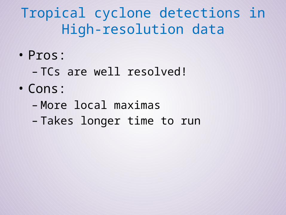
Tropical cyclone detections in High-resolution data

• Pros: – TCs are well resolved!

• Cons:– More local maximas– Takes longer time to run

Characteristics of a Tropical cyclones

• Large negative sea level pressure deficit• Warm cored structure – positive temperature

anomaly through out the troposphere.• Large (tangential) wind speed (Vm>17ms-1) • Large vorticity

Our last TC detect procedure

1 Compute U, V, T, H at specific pressure level (850hPa, 700hPa, 500hPa, 300hPa and Sea Level Pressure)

Check each grid point for TC candidate: A vorticity maxima at 850hPa that has value greater than a prescribed criteria (e.g. 10-4 s-1) (10-5 s-1)

2

3Search for the SLP minimum center using birational interpolation (within 2 degree radius circle from Candidate center)

Our last TC detect procedure (cont.)

4 Check Criteria to determine a Tropical Cyclone

1o2.5o Outer Core Streng (OCS) at 850hPa > OCSCrit (10 ms-1) (5 ms-1)

2.5o

SLP Anomaly < SLPCrit (-2 hPa)Core Temperature Anomaly > TcoreCrit (1 K)

Geopotential Height Anomaly at 500hPa < H500Crit (-10m)

Core Temperature Anomaly is calculated by weighted averaging (0.1, 0.2, 0.3, 0.4)

Tracking procedure:

Is the dectected TC a new born one or a previous one?

t0 - 12h

t0 - 6h

300km

Final processing: only vortices that lasts at least two days are considered to be model TCs.

Some thoughts

• The detection time is quite long (mainly because of the costly interpolation procedure)

• Higher resolutions lead to more small-scale spatial variation of vorticity, these maxima are not located at the centers

• Sea level pressure is somewhat more reliable because its variation is quite small

• Is the searching for vorticity maxima at the first place necessary?

• Or is it necessary at all in the whole procedure?

Criteria?

Vorticity?

- At 850 hPa, 900 hPa- Threshold: >1 × 10-5, 2.0 × 10-5, 3.5 × 10-5, 3.5 × 10-5, 7 × 10-5,

For more detail, see Walsh et al. (2006)

Others

- Latitude < 30o ,40o

- Cannot genesis on land

Wind speed?

- At 850 hPa, at 10m- Area-averaged, OCS- Threshold: >5ms-1, 10ms-1, 15ms-1, 17ms-1,

Warm cored structure?

- T’250 > 0.5K- T’700 + T’500 + T’300 > 0 K, 1.5K, 3K-T’850 +T’700 + T’500 + T’300 > 3

Minimum lifespan

1, 2, 3 days

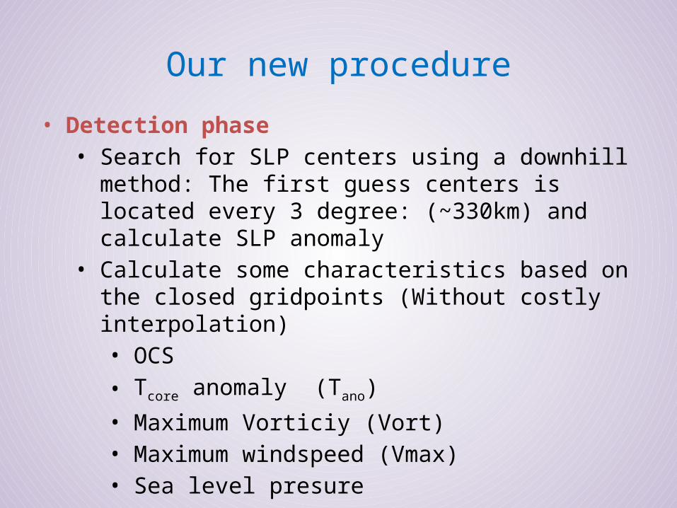
Our new procedure

• Detection phase• Search for SLP centers using a downhill method: The

first guess centers is located every 3 degree: (~330km) and calculate SLP anomaly

• Calculate some characteristics based on the closed gridpoints (Without costly interpolation)• OCS

• Tcore anomaly (Tano)

• Maximum Vorticiy (Vort)• Maximum windspeed (Vmax)• Sea level presure

Our new procedure

• Tracking phase• If two centers are close (e.g. less than 400km), only

the one with lower SLPano is chosen.• The tracking procedure is similar to the previous

one.

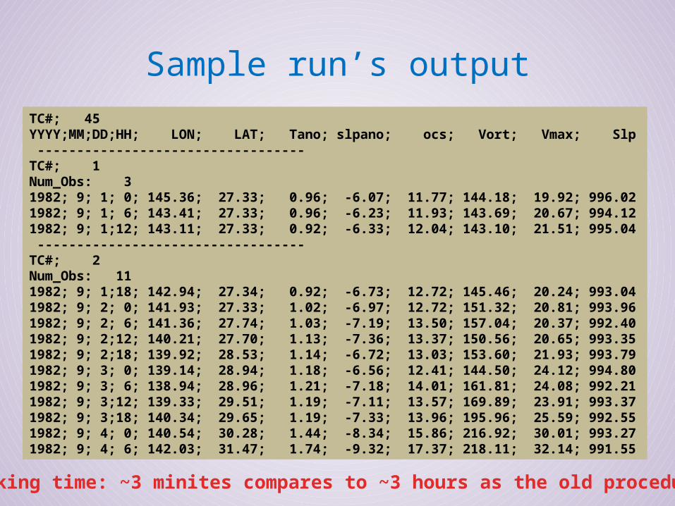
Sample run’s outputTC#; 45YYYY;MM;DD;HH; LON; LAT; Tano; slpano; ocs; Vort; Vmax; Slp ----------------------------------TC#; 1Num_Obs: 31982; 9; 1; 0; 145.36; 27.33; 0.96; -6.07; 11.77; 144.18; 19.92; 996.021982; 9; 1; 6; 143.41; 27.33; 0.96; -6.23; 11.93; 143.69; 20.67; 994.121982; 9; 1;12; 143.11; 27.33; 0.92; -6.33; 12.04; 143.10; 21.51; 995.04 ----------------------------------TC#; 2Num_Obs: 111982; 9; 1;18; 142.94; 27.34; 0.92; -6.73; 12.72; 145.46; 20.24; 993.041982; 9; 2; 0; 141.93; 27.33; 1.02; -6.97; 12.72; 151.32; 20.81; 993.961982; 9; 2; 6; 141.36; 27.74; 1.03; -7.19; 13.50; 157.04; 20.37; 992.401982; 9; 2;12; 140.21; 27.70; 1.13; -7.36; 13.37; 150.56; 20.65; 993.351982; 9; 2;18; 139.92; 28.53; 1.14; -6.72; 13.03; 153.60; 21.93; 993.791982; 9; 3; 0; 139.14; 28.94; 1.18; -6.56; 12.41; 144.50; 24.12; 994.801982; 9; 3; 6; 138.94; 28.96; 1.21; -7.18; 14.01; 161.81; 24.08; 992.211982; 9; 3;12; 139.33; 29.51; 1.19; -7.11; 13.57; 169.89; 23.91; 993.371982; 9; 3;18; 140.34; 29.65; 1.19; -7.33; 13.96; 195.96; 25.59; 992.551982; 9; 4; 0; 140.54; 30.28; 1.44; -8.34; 15.86; 216.92; 30.01; 993.271982; 9; 4; 6; 142.03; 31.47; 1.74; -9.32; 17.37; 218.11; 32.14; 991.55

Tracking time: ~3 minites compares to ~3 hours as the old procedure

Some initial results

• Simulation data: CCAM simulation for 09/1982.• Stretching grid, highest resolution: ~20km over

the region of Vietnam• Spectral nudging from ERA-interim

Some initial results

Observation (ibtracs)

Case 1 SLPCrit = -3hPa

Min life span = 8

OCSCrit= 3 m/s TcoreCrit = 0

Case 1 SLPCrit = -3hPa

Min life span = 1

OCSCrit= 3 m/s TcoreCrit = 0

SLP vs Tcore_anom

0

0.5

1

1.5

2

2.5

3

3.5

4

4.5

5

-20 -15 -10 -5 0

TC

Non_TC

K

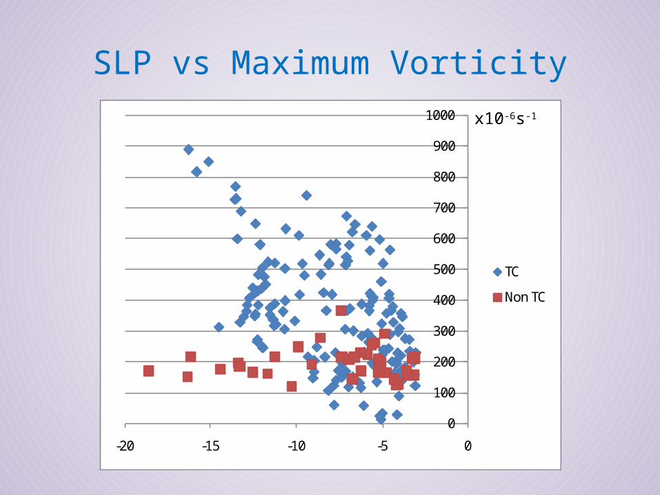
SLP vs Maximum Vorticity

0

100

200

300

400

500

600

700

800

900

1000

-20 -15 -10 -5 0

TC

Non TC

x10-6s-1

SLP vs OCS

0

5

10

15

20

25

30

-20 -15 -10 -5 0

TC

Non_TC

ms-1

SLPmin vs OCS and Vmax

0

5

10

15

20

25

30

35

40

45

50

980 990 1000 1010 1020

Vmax

Vmax

0

5

10

15

20

25

30

35

40

45

50

980 990 1000 1010 1020

OCS

OCS

Correl = -0.85 Correl = -0.71

Increasing the OCS criteria

OCSCrit = 3m/s OCSCrit = 6m/s

Increasing the OCS criteria

OCSCrit = 3m/s OCSCrit = 6m/s

Conclusion and remarks

• High resolution’s data has some challenges for Tropical cyclone detection procedures

• Vorticity doesn’t seem to be a good criteria for Tropical cyclone detection

• OCS in the model is highly correlated with intensity (SLV), not like in observation. The reason may be model TCs are broader.

• Future works: • Have some case studies with ‘regular’ 50-km or

possibly higher resolution.• Improve the tracking precedure

Thanks for your attention!