Journal of Sound and Vibration (1996) 191(1), 91–106

A NEW HIGH-ORDER NON-UNIFORMTIMOSHENKO BEAM FINITE ELEMENT ON

VARIABLE TWO-PARAMETER FOUNDATIONSFOR VIBRATION ANALYSIS

Y. C. H C. H. T

Department of Mechanical Engineering, National Chiao Tung University,1001 Ta Hsuen Rd., Hsinchu, Taiwan, Republic of China

S. F. L

School of Mechanical and Production Engineering, Nanyang TechnologicalUniversity, Nanyang Avenue, Singapore

(Received 9 August 1994, and in final form 13 February 1995)

A new finite element model of a Timoshenko beam is developed to analyze the smallamplitude, free vibrations of non-uniform beams on variable two-parameter foundations.An important characteristic of the model is that the cross-sectional area, the secondmoment of area, the Winkler foundation modulus and the shear foundation modulus areall assumed to vary in polynomial forms, implying that the beam element can deal withcommonly seen non-uniform beams having different cross-sections such as rectangular,circular, tubular and even complex thin-walled sections as well as the foundation of beamswhich vary in a general way. Thus this new beam element model enables users to handlevibration analysis of more general beam-like structures. In this paper, by using cubicpolynomial expressions for the total deflection and the bending slope of the beam, the massand stiffness matrices of the element are derived from energy expressions. The elementmodel can accommodate various boundary conditions to represent a Timoshenko beamaccurately. Excellent agreement with other investigators’ results and a rapid rate ofconvergence with relatively few elements are demonstrated. This study also brings out thefact that the complicated form of this new beam model is necessary because of its advantageover linear or uniform approximations of the non-uniform foundation and/or geometricalproperties of beams. The same accuracy being achieved with fewer elements is the mainadvantage. Finally, an optimum design problem is illustrated to emphasize the practicalapplication of this element.

71996 Academic Press Limited

1. INTRODUCTION

Beams resting on elastic foundations are very common in structural systems. Many authorshave proposed mathematical models to simulate such structural systems. In these studies[1–4] the foundation is usually modelled on the basis of the well-known Winkler hypothesiswhich postulates that a foundation behaves like an infinite series of closely spaced,independent, linearly elastic, vertical springs. The limitation of these models is that theyassume no interaction between the springs, so the models fail to reproduce thecharacteristics of a continuous medium. To overcome this problem, two-parameter models(or Pasternak models) were developed to couple the response within the foundation.

91

0022–460X/96/110091+16 $18.00/0 7 1996 Academic Press Limited

. . .92

Mathematically all these models are equivalent, differing only in their definitions of thefoundation parameters. Using the Bernoulli–Euler beam theory, Valsangkar andPradhanang [5] investigated the influence of foundation continuity (or a partially elasticfoundation) on the natural frequencies of beam-columns resting on constanttwo-parameter models. Eisenberger and Clastornik [6, 7] and Clastornik et al. [8] havestudied vibrations and buckling of beams on variable Winkler and two-parameterfoundations. Other authors [9–12] have solved similar problems in which the effects ofshear deformation and rotatory inertia on the natural frequencies of the beam wereincluded (in other words, based on the Timoshenko beam theory).

In many engineering applications, non-uniform beams with cross-sections varying in acontinuous or non-continuous manner along their lengths are used in an effort to achievean optimum distribution of strength and weight. Extensive work has been done on thevibration of a non-uniform beam. With the effects of shear deformation and rotatoryinertia included, the finite element approach to this problem has been shown successfullyin several published studies [13–15]. Chehil and Jategaonkar [16] used the Galerkin methodto estimate the first few natural frequencies of a simple-supported beam with varyingsection properties. They have also evaluated the natural frequencies of a non-uniformbeam with varying cross-section in a continuous or non-continuous manner along itslength under other classic boundary conditions [17]. Recently, by using the homogeneoussolutions of the governing equations for static deflections as the shape functions, Cleghornand Tabarrok [18] developed a finite element model for free lateral vibration analysis oflinearly tapered Timoshenko beams. However, the mass matrix they derived is onlyapproximate, although the stiffness matrix is exact. Tang [19] derived a second-orderfinite element formulation of linearly tapered beam-column elements. In their work,different tapering types such as width changing only, height changing only, width andheight changing at the same rate and a different rate for various section shapes wereconsidered.

From the above survey, it is found that part of the work has been focused on theproblem of a uniform beam resting on a constant or variably elastic foundation. As tothe field of vibration of non-uniform beams, the situation where non-uniform beams arefully or partially embedded on elastic foundations is less well-explored. It is well knownthat the governing equation for uniform foundations has constant coefficients andanalytical solutions of it can be obtained. But if the foundations vary along the beams,in most cases the governing equation cannot be solved exactly, so numerical techniquesmust be applied. Therefore, the purpose of the present paper is to develop a new finiteelement model to determine the natural frequencies of a non-uniform Timoshenko beamresting on a variable two-parameter foundation. The effects of non-linearly taperedcross-sectional area, variable two-parameter foundations, fully or partially, sheardeformation, and rotatory inertia are all taken into account in this new beam elementmodel. The taper type is considered as the cross-sectional area and second moment of areaare expressed in polynomial forms. The variable two-parameter foundation also ispostulated to be of polynomial form. This element model thus allows the inertia, cross-sectional area and the elastic foundation to vary in a general manner. Cubic polynomialsoriginally suggested by Thomas [20] are employed here for the element model with the totaldeflection, c, total slope, c', bending slope, f, and the first derivative of bending slope,f' as nodal co-ordinates. By using the Lagrange principle, the stiffness and mass matricesfor small amplitude, free vibrations of the beam are derived from energy expressions andthe governing matrix equation is then obtained after assembling element stiffness and massmatrices. This model is capable of accommodating various boundary conditions such as:(a) free end–zero bending moment and zero shear force; (b) fixed end–zero total deflection

93

and zero bending slope; (c) hinged end–zero total deflection and zero bending moment,thus representing a Timoshenko beam accurately. Numerical results based on this newbeam element model are compared with those presented by various researchers to verifythe accuracy of the model. This study also brings out the fact that the complicated formof this new beam model is necessary because of its advantage over linear or uniformapproximations of the non-uniform foundation and/or geometrical properties of beams.The use of fewer elements to achieve the same accuracy is the main advantage, as theamount of numerical calculation required is thereby reduced. Finally, an optimum designproblem is illustrated to emphasize the practical application of this element.

2. DERIVATION OF ELEMENT MATRICES

The new Timoshenko beam element model with cross-section varying in a continuousmanner along its length l is shown in Figure 1. Cross-sectional area Ae(x) and secondmoment of area Ie(x) are described in the polynomial forms (see Appendix B fornomenclature)

Ae(x)=sn2

i=0

Bixi, Ie(x)=sn1

i=0

Aixi, (1, 2)

where x represents the co-ordinate along the beam. The variable two-parameter elasticfoundation is represented as a general polynomial in x: i.e., the varying elastic foundation,

Figure 1. The beam model. (a) Beam element; (b) definition of the nodal co-ordinates.

. . .94

characterized by two moduli, the Winkler foundation modulus ket (x) and the shear

foundation modulus kes (x), are also described in polynomial forms:

ket (x)=s

n3

i=0

Cixi, kes (x)=s

n4

i=0

Dixi, (3, 4)

Basis assumptions for the present Timoshenko beam element are as follows: (i) the beammaterial is isotropic, homogeneous and linearly elastic; (ii) the vibration amplitude of thebeam is sufficiently small; (iii) the cross-section initially normal to the neutral axis of thebeam remains plane, but no longer normal to that axis after bending; (iv) the dampingis negligible.

The potential energy Ue of the beam element of length l including the effects of bothshear deformation and elastic foundation is given by

Ue=12

Egl

0

Ie(x) 01f

1x12

dx+12

kG gl

0

Ae(x) 01y1x

−f12

dx+12 g

l

0

ket (x)y2 dx

+12 g

l

0

kes (x) 01y

1x12

dx. (5)

By substituting h=x/l and c=y/l, Ue can be non-dimensionalized as

Ue=12

El g

l

0

Ie(h) 01f

1h12

dh+12

kGl gl

0

Ae(h) 01c

1h−f1

2

dh+12

l3 gl

0

ket (h)c2 dh

+12

l gl

0

kes (h) 01c

1h12

dh, (6)

where c, c', f and f' representing the total deflection, total slope, bending slope, andthe first derivative of bending slope, respectively, are the four-degrees-of-freedom at eachnode, and Ae(h), Ie(h), ke

t (h) as well as kes (h) take the following forms:

Ae(h)=sn2

i=0

bihi, Ie(h)=s

n1

i=0

aihi, ke

t (h)=sn3

i=0

ktihi, ke

s (h)=sn4

i=0

ksihi, (7–10)

For a uniform beam, it is worth noting that n1=n2=0, thus leading to Ae=b0 and Ie=a0.By using a cubic polynomial distribution for c and f, i.e.

c=s3

i=0

aihi, f=s

3

i=0

bihi, (11, 12)

and expressing the coefficients ai and bi in terms of nodal values c, c', f and f' at thenodes i and i+1 (the prime denotes differentiation with respect to h), the followingequations can be obtained:

c=[N1 N2 N3 N4]GG

G

K

k

ci

c'ici+1

c'i+1

GG

G

L

l, f=[N1 N2 N3 N4]G

G

G

K

k

fi

f'ifi+1

f'i+1

GG

G

L

l. (13, 14)

95

N1–N4 are the shape functions and have the following forms

N1=1−3h2+2h3, N2=h−2h2+h3, N3=3h2−2h3, N4=−h2+h3.

(15–18)

Upon substituting equations (13)–(18) into equation (6), the strain energy becomes

Ue=(E/2l){je}T[Ke]{ze}, (19)

where {ze}T={ci fi c'i f'i ci+1 fi+1 c'i+1 f'i+1}. The terms of [Ke] are given inAppendix A.

The kinetic energy Te of this beam element can be written as

Te=12

r gl

0

Ae(x) 01y1t1

2

dx+12

r gl

0

Ie(x) 01f

1t12

dx. (20)

After non-dimensionalization, Te becomes

Te=12

rl3 gl

0

Ae(h) 01c

1t12

dh+12

rl gl

0

Ie(h) 01f

1t12

dh. (21)

With the help of equations (13)–(18), Te can be written in the form

Te=12rl3{z� e}T[Me]{z� e}, (22)

in which the dot indicates differentiation with respect to time. The entries of [Me] are alsolisted in Appendix A. Furthermore, when the beam is not embedded on elasticfoundations, ke

t=kes=0. In this case, the element matrices [Ke] and [Me] derived here will

reduce to the forms presented by Thomas [20].Applying Lagrange’s principle to the sum of individual element energies over the whole

beam gives the dynamic equilibrium equation for small amplitude free vibration of anon-uniform Timoshenko beam on a two-parameter elastic foundation as

[K]{j}+(rl4/E)[M]{z� }={0}, (23)

where

[K]=se

[Ke], [M]=se

[Me], {j}=se

{ze}, (24)

are the global stiffness matrix, the global consistent mass matrix, and the globaldisplacement vector assembled by adding the contributions from all the elements,respectively. For the operations in equations (24), the matrix or vector on the right mustbe expanded with zero to make it the same size as the matrix or vector on the left. When{z} is harmonic in time with circular frequency v, equation (23) takes the standardeigenvalue problem form

([K]−l4[M]){z� }={0}, (25)

where {z}={z� }exp(ivt) and l4=v2rl4/E. Thus the non-trivial solution of equation (25)gives the natural frequencies and the corresponding mode shapes.

. . .96

T 1

Basic parameters used in the first two numerical examples

n 1/3G/E 3/8k 2/3L 25b0 1

bi ,i=1,...,n2 0a0 1

ai ,i=1,...,n1 0kti ,i=1,...,n3 0

Kt kt0L4/Ea0

ksi ,i=1,...,n4 0Ks ks0L2/Ea0

C4 v2rb0L4/Ea0

3. ILLUSTRATIVE EXAMPLES AND DISCUSSION

In this section, the first three numerical examples are presented to demonstrate theaccuracy and convergence rate of the new element model by comparing results with thoseof other authors. Data used in this example, which were presented by Yokoyama [11], aresummarized in Table 1. The structure studied in the first example is a uniformhinged–hinged beam fully supported on a constant two-parameter foundation. It shouldbe noted that, for such a structure, equations (7)–(10) reduce to Ae=b0, Ie=a0, ke

t=kt0,and ke

s=ks0, representing the fact that the cross-sectional area, the second moment of areaof the beam and the foundation are all constants. With foundation parametersKt=kt0L4/Ea0 and Ks=ks0L2/Ea0 varying from 1 to 104 and 0 to 2.5p2, respectively, Table 2compares the first three frequency parameters calculated here with exact solutionscomputed from the frequency equations reported in reference [9] and results presented byYokoyama [11]. The exact solutions reported in reference [9] were obtained from thecoupling differential equations for transverse vibrations of uniform Timoshenko beams on

T 2

Comparison of the frequency parameter C of the first three modes of a uniformhinged–hinged Timoshenko beam fully supported on a two-parameter foundation

Presentno. of d.o.f.s

Exact Reference [11]Mode [9] 64 d.o.f.s 8 12 20

Kt=1 Ks=0 1 3·092 3·09 3·094 3·092 3·0922 5·881 5·88 5·970 5·888 5·8823 8·301 8·31 8·946 8·373 8·305

Ks=2·5p2 1 4·267 4·27 4·268 4·267 4·2672 6·795 6·80 6·862 6·800 6·7963 9·085 9·09 9·632 9·148 9·088

Kt=104 Ks=0 1 9·984 9·98 9·985 9·985 9·9842 10·187 10·19 10·204 10·188 10·1873 10·903 10·90 11·220 10·935 10·905

Ks=2·5p2 1 10·044 10·04 10·044 10·044 10·0442 10·400 10·40 10·419 10·401 10·4003 11·278 11·28 11·588 11·311 11·280

97

T 3

Comparison of the fundamental frequency parameter C of a uniform Timoshenko beamfully supported on a two-parameter foundation

Presentno. of d.o.f.s

Exact ReferenceL2 [9] [12] 8 16

Hinged–hinged beamKt=Ks=0 50 2·735 2·740 2·735 2·735

4000 3·134 3·135 3·141 3·134Kt=Ks=25 50 4·170 4·194 4·170 4·170

4000 4·378 4·379 4·381 4·379Clamped–clamped beam

Kt=Ks=0 50 3·305 3·318 3·306 3·3054000 4·682 4·691 4·712 4·684

Kt=Ks=25 50 4·439 4·443 4·440 4·4394000 5·324 5·324 5·367 5·326

constant elastic foundations. Yokoyama presented approximate solutions obtained froma beam model developed by himself, in which beams and their foundations (if any) areboth restricted to be of uniform forms. As shown in Table 2, by comparing with the exactsolutions, to attain the same level of numerial error, only 20 d.o.f.s (degrees-of-freedom),i.e., five elements, are sufficient in the present model but 64 d.o.f.s are used in Yokoyama’smodel. It should also be noted that the present results with 12 d.o.f.s approach those with20 d.o.f.s very closely. The above numerical results reveal that the rate of convergence ofthe present model is more rapid than that of Yokoyama’s model without losing accuracyas the number of degrees-of-freedom increases.

Under the conditions used by Filipich [12], the second example again verifies the beamelement model developed here. As with the similar structure studied in the first example,data are the same as those listed in Table 1, except k=1 and G/E=9/28. This exampleconsiders two types of boundary conditions, hinged–hinged and clamped–clamped, underseveral different sets of Kt , Ks , and L. Table 3 shows the comparison of results calculatedfor the fundamental frequency parameters with the corresponding exact solutions [9] andapproximate solutions obtained by Filipich [12], who used a variant of Rayleigh’s methodto determine the natural frequencies. For both hinged–hinged and clamped–clampedboundary conditions with various Kt , Ks , and L, the accuracy of the present beam modelis again demonstrated because the results obtained with 16 d.o.f.s in the present modelapproach the exact solutions and those presented by Filipich very closely. From Table 3,one can observe that the present results based on 8 d.o.f.s and 16 d.o.f.s are almost thesame; thus the convergence rate of this new beam model is further demonstrated.

The third example is a case of a hinged–hinged rectangular cross-section beam of linearlyvarying width and depth, giving rise to non-linear variations in both the cross-sectionalarea and second moment of area. Basic data and comparison results are shown in Table 4.From Table 4, it is apparent that the discrepancy between the numerical results presentedby Jategaonkar [17] and the results based on the proposed model is relatively small. Thusthe accuray of the present model is demonstrated for the case of non-uniform beams.

Usually, while analyzing the dynamic beahviour of non-unfirom beams on foundationsvarying in a general form, cross-sections and foundations are approximated to changelinearly or to be distributed uniformly in order to simplify the analysis. If such

. . .98

approximations work well in most cases, the need for the derivation of this new beamelement model is doubtful due to its complex and lengthy form, which users may feel isdifficult to use. In this example therefore, the necessity of using the exact forms of variationon foundations and cross-sections instead of using the linear approximation is presented.Consider a non-uniform free–free beam resting on a variable two-parameter foundation.The original forms of kt (x), ks (x) are assumed in this example to be

kt (x)=(c1−c2)(1−x/L)3+c2, ks (x)=(c3−c4)(1−x/L)3+c4, (26, 27)

and the cross-section is assumed to be rectangular with width b(x) and depth h(x) varyingas

b(x)=[(x/L)+c5]3, h(x)=[(x/L)+c6]3. (28, 29)

When using the linear approximation, values of kt (x), ks (x), b(x), and h(x) on nodal pointsare obtained from equations (26)–(29) and set to vary linearly within each element. Basedon the values of parameters given in Table 5, Figure 2 shows the first three calculatednatural frequencies obtained from the original forms and from the linear approximationof the cross-section and foundation. The results obtained based on the original forms ofkt (x), ks (x), b(x), and h(x), have nearly converged with four elements, but those with thelinear approximation apparently converge very slowly. This shows the superior rate of

T 4

Comparison of the natural frequency vn(rad/s) of a Timoshenko beamwith both cross-sectional area and second moment of area

non-linearly varying

Presentno. of d.o.f.s

Mode Reference [17] 24 32

1 6·56 6·259 6·2592 22·68 21·979 21·9753 47·09 46·463 46·4354 73·95 74·222 74·1125 103·14 105·219 104·811

99

T 5

Values of parameters used in Figure 2

n 0·3E 3×106

r 1k 0·85L 9c1 108

c2 101

c3 108

c4 101

c5 0·9c6 0·9

convergence of the natural frequencies based on the exact forms given in equations(26)–(29). Therefore, one can draw the conclusion that using foundation and cross-sectionforms that exactly match the original ones has an advantage over the linear approximationin that fewer elements are needed to achieve the same accuracy, thus reducing the amountof numerical calculation required.

Figure 2. The first three circular frequencies as functions of the number of elements for a free–free non-uniformTimoshenko beam resting on a variable two-parameter foundation. ——, Original forms of equations (26)–(29);---, linear approximation to the original forms.

. . .100

Figure 3. A beam partially embedded in a two-parameter foundation and subjected to external stationaryloading P(t).

The final example is of an optimum design problem, to illustrate the practical applicationof this new beam element model. As shown in Figure 3, a beam with circular cross-sectionis partially embedded on a variable two-parameter foundation and subjected to astationary load P(t). Data employed in the example are E=210 GPa, n=0·3, k=0·85,r=7840 kg/m3, L=0·5 m, Lb=0·2 m and b0=0·01p m2. The moduli of the foundation are

kt (x)=(108−10)(1−x/Lb )3+10 (N/m2), ks (x)=106(x/Lb ) (N). (30, 31)

The target of the design is to determine the profile of the beam needed to minimize theweight. Two frequecy constraints are specified. The first constraint requires that the firstnatural frequency be greater than 8 Hz and less than 14 Hz. The second constraintdemands the second natural frequency to be greater than 60 Hz and less than 65 Hz. Thesefrequency constraints ensure that the resonance response will not appear because P(t)contains less energies in these frequency ranges. Assume the cross-sectional area varies as

A(x)=b0+b1(x/L)+b2(x/L)2+b3(x/L)3 (m2). (32)

Therefore, the second moment of area I(x) is

I(x)=[b0+b1(x/L)+b2(x/L)2+b3(x/L)3]2/4p (m4). (33)

The optimum design problem can be stated as follows. Minimize an objective function

f(x)=gL

0

rA(x) dx (34)

subject to

8 HzEf1E14 Hz, 60 HzEf2E65 Hz. (35, 36)

In this example, three sets of design variables x are chosen:Case 1: x={b1}, i.e., b1 is the design variable, b2 and b3 are assigned to be zero;Case 2: x={b1 b2}, b1 and b2 are the design variables, b3 is set to be zero;Case 3: x={b1 b2 b3}, b1, b2 and b3 are all design variables.

In case 1 the cross-section of the beam varies in a linear way. For case 2 one assumesthat the cross-section varies as a second order polynomial along the beam. Similarly, thecross-section varies as a third order polynomial in case 3. Five elements are used in the

101

T 6

Design bounds and initial values of design variables

Case Design Initial Lower Upperno. variables values bound bound

1 b1 0 −0·01p 12 b1 0 −0·01p 1

b2 0 −0·01p 13 b1 0 −0·01p 1

b2 0 −0·01p 1b3 0 −0·01p 1

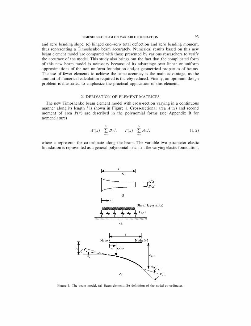
associated finite element model with two of these elements resting on the foundation. Theoptimum problem is solved with the help of the (sequential quadratic programming) SQPmethod [21]. The original design has a uniform beam so that A(x)=0·01 p m2, f1=12·3 Hz,f2=57·5 Hz, and the mass=123·2 kg. The designer wishes to adjust the natural frequenciesby changing the beam mass so that resonance will not appear. Table 6 lists the designbounds and initial values of the design variables adopted in the optimum numericalalgorithm for each design case. The final results of optimum design are shown in Table 7,from which it can be seen that the first two natural frequencies have been adjustedadequately by satisfying the constraints. In each case, f1 stays finally at its upper bound,which means that for this formulation of the optimum problem, the minimum beam massis obtained when either f1 or f2 reach their upper bound first. By comparing the optimumresults obtained in the three design cases, case 3 in which the cross-section is assumed tovary as a third-degree polynomial gives a beam mass of 90 kg, a maximum reduction ofmass in the three cases nearly equal to 33 kg. From the standpoint of the optimum designconcept, the better design obtained in case 3 implies that one can search for the optimumpoint more extensively due to the design space being enlarged.

4. CONCLUSIONS

A new Timoshenko beam finite element has been developed for the analysis of smallamplitude, free vibration of non-uniform beams on variable two-parameter foundation.The cross-sectional area, the second moment of area of the beam as well as the foundationsare all assumed to be polynomial forms, so that the beam model is the only one presentedso far which is suitable for general types of beams and foundations. Other advantages ofthis beam element include (i) the convergence rate of results obtained from this model is

T 7

Optimum results of the design problem in the final example

Optimum results

Case no. Design variables f1(Hz) f2(Hz) Mass (kg)

b1 b2 b3

1 −9·426×10−3 – – 14·0 60·23 104·72 −3·140×10−2 2·763×10−2 – 14·0 62·43 97·73 −3·140×10−2 −3·140×10−2 7·084×10−2 14·0 63·95 90·0

12·3* 57·50* 123·2*

* Denotes the original design (based on a uniform beam).

. . .102

rapid; (ii) use of a relatively small number of elements can obtain accurate results; (iii) bothgeometric and free boundary conditions can be applied correctly, according to thecomparison results obtained in the first four examples. Therefore a Timoshenko beam canbe represented accurately. The final example of an optimum design problem illustrates thepractical appliation of this new beam element model. By using the new beam elementmodel to build up a finite element model as an analysis tool, a precise profile of the beamstructure is then determined while the mass of the beam is minimized and frequencyconstraints are satisfied.

ACKNOWLEDGMENTS

The authors acknowledge the support of this work by the National Science Council,Taiwan, R.O.C., under grant NSC82-0401-E009-085.

REFERENCES

1. P. F. D and M. N. P 1982 Earthquake Engineering and Structural Dynamics 10,663–674. Vibration of beams on partially elastic foundations.

2. M. E, D. Z. Y and M. A. A 1985 Earthquake Engineering andStructural Dynamics 13, 651–660. Vibrations of beams fully or partially supported on elasticfoundations.

3. P. A. A. L and V. H. C 1987 Journal of Engineering Mechanics, American Societyof Civil Engineers 113, 143–147. Vibrating beam partially embedded in Winkler-type foundation.

4. A. J. V and R. B. P 1987 Journal of Engineering Mechanics, AmericanSociety of Civil Engineers 113, 1244–1247. Free vibrations of partially supported piles.

5. A. J. V and R. P 1988 Earthquake Engineering and Structural Dynamics16, 217–225. Vibrations of beam-columns on two-parameter elastic foundations.

6. M. E and J. C 1987 Journal of Sound and Vibration 115, 233–241.Vibrations and buckling of a beam on a variable Winkler elastic foundation.

7. M. E and J. C 1987 Journal of Engineering Mechanics, American Societyof Civil Engineers 113, 1454–1466. Beams on variable two-parameter elastic foundation.

8. J. C, M. E, D. Z. Y and M. A. A 1986 Journal of AppliedMechanics 53, 925–928. Beams on variable Winkler elastic foundation.

9. T. M. W and J. E. S 1977 Journal of Sound and Vibration 51, 149–155. Naturalfrequencies of Timoshenko beams on Pasternak foundations.

10. T. M. W and L. W. G 1978 Journal of Sound and Vibration 59, 211–220. Vibrationsof continuous Timoshenko beams on Winkler–Pasternak foundations.

11. T. Y 1991 Earthquake Engineering and Structural Dynamics 20, 355–370. Vibrationsof Timoshenko beam-columns on two-parameter elastic foundations.

12. C. P. F and M. B. R 1988 Journal of Sound and Vibration 124, 443–451. A variantof Rayleigh’s method applied to Timoshenko beams embedded in a Winkler–Pasternak medium.

13. T. I, G. Y and I. T 1979 Journal of Sound and Vibration 63, 287–295.Determination of the steady state response of a Timoshenko beam of varying cross-section byuse of the spline interpolation technique.

14. C. W. S. T 1979 Journal of Sound and Vibration 63, 33–50. Higher order taper beam finiteelements for vibration analysis.

15. C. W. S. T 1981 Journal of Sound and Vibration 78, 475–484. A linearly tapered beam finiteelement incorporating shear deformation and rotary inertia for vibration analysis.

16. D. S. C and R. J 1987 Journal of Sound and Vibration 115, 423–436.Determination of natural frequencies of a beam with varying section properties.

17. R. J and D. S. C 1989 Journal of Sound and Vibration 133, 303–322. Naturalfrequencies of a beam with varying section properties.

18. W. L. C and B. T 1992 Journal of Sound and Vibration 152, 461–470. Finiteelement formulation of a tapered Timoshenko beam for free lateral vibration analysis.

19. X. T and B. T 1993 Computers and Structures 46, 931–941. Second-order taperedbeam-column elements.

103

20. J. T and B. A. H. A 1975 Journal of Sound and Vibration 41, 291–299. Finite elementmodel for dynamic analysis of Timoshenko beam.

21. C. H. T, W. C. L, and T. C. Y 1993 Technical Report No. AODL-93-01, Departmentof Mechanical Engineering, National Chiao Tung University. 1.1 user’s manual.

APPENDIX B: NOMENCLATURE

Ae cross-sectional area of the element eIe second moment of area of the element eE Young’s modulus of beam materialG shear modulus of beam materialk shear coefficientr mass density of the materialL entire length of beamLb length of the part of the beam resting on a foundationl element lengthTe kinetic energy of the beam element eUe strain energy of the beam element ex co-ordinate along the axis of the beamy deflection of the centroid of the beamf bending slopeh x/l, non-dimensional co-ordinatec y/l, non-dimensional deflectionv angular frequency of beam vibrationke

t Winkler foundation modulus of the beam element eke

s shear foundation modulus of the beam element eAi coefficients representing the variations in Ie(x)Bi coefficients representing the variations in Ae(x)Ci coefficients representing the variations in ke

t (x)Di coefficients representing the variations in ke

s (x)ai coefficients representing the variations in Ie(h)bi coefficients representing the variations in Ae(h)kti coefficients representing the variations in ke

t (h)ksi coefficients representing the variations in ke

s (h)n1 order of the polynomial form which describes Ie

n2 order of the polynomial form which describes Ae

n3 order of the polynomial form which describes ket

n4 order of the polynomial form which describes kes

APPENDIX A

The entries of [Ke] are given as follows:

k11=sn2

i=0

72biSC1

+72l4

Esn3

i=0

kti (13+3i)C6

+72l2

Esn4

i=0

ksi

C1, k12=36 s

n2

i=0

bi (10+3i)SC2

,

k13=12 sn2

i=0

bi (1+2i)SC3

+24l4

Esn3

i=0

kti (l+3i)C8

+12l2

Esn4

i=0

ksi

C3, k14=36 s

n2

i=0

biSC4

,

k15=−72 sn2

i=0

biSC1

+6l4

Esn3

i=0

kti (54+17i+i2)C9

−72l2

Esn4

i=0

ksi

C1, k16=6 s

n2

i=0

bi (10+i)SC5

,

. . .104

k17=6 sn2

i=0

bi (1−i)SC1

−6l4

Esn3

i=0

kti (13+3i)C9

+6l2

Esn4

i=0

ksi (1−i)C1

, k18=−12 sn2

i=0

biSC5

,

k22=72 sn2

i=0

bi (13+3i)SC6

+72 sn1

i=0

ai

C1, k23=12 s

n2

i=0

bi (−2+3i)SC7

,

k24=24 sn2

i=0

bi (11+3i)SC8

+12 sn1

i=0

ai (1+2i)C3

, k25=−36 sn2

i=0

bi (10+3i)SC2

,

k26=6 sn2

i=0

bi (54+17i+i2)SC9

−72 sn1

i=0

ai

C1, k27=6 s

n2

i=0

bi (12−i2)SC2

,

k28=−6 sn2

i=0

bi (13+3i)SC9

+6 sn1

i=0

ai (1−i)C1

,

k33=8 sn2

i=0

bi (2+i2)SC10

+24l4

Esn3

i=0

kti

C9+

8l2

Esn4

i=0

ksi (2+i2)C10

, k34=12 sn2

i=0

biiSC2

,

k35=−12 sn2

i=0

bi (1+2i)SC3

+2l4

Esn3

i=0

kti (13+i)C11

−12l2

Esn4

i=0

ksi (1+2i)C3

,

k36=2 sn2

i=0

bi (18+2i+i2)SC4

,

k37=−2 sn2

i=0

bi (2+i2)SC3

−6l4

Esn3

i=0

kti

C11−

2l2

Esn4

i=0

ksi (2+i2)C3

,

k38=−2 sn2

i=0

bi (3+2i)SC4

, k44=24 sn2

i=0

biSC9

+8 sn1

i=0

ai (2+i2)C10

,

k45=−36 sn2

i=0

biSC4

, k46=2 sn2

i=0

bi (13+i)SC11

−12 sn1

i=0

ai (1+2i)C3

,

k47=2 sn2

i=0

bi (3−i)SC4

, k48=−6 sn2

i=0

biSC11

−2 sn1

i=0

ai (2+i2)C3

k55=72 sn2

i=0

biSC1

+l4

Esn3

i=0

kti (78+17i+i2)C12

+72l2

Esn4

i=0

ksi

C1, k56=−6 s

n2

i=0

bi (10+i)SC5

,

k57=6 sn2

i=0

bi (−1+i)SC1

−l4

Esn3

i=0

kti (11+i)C12

+6l2

Esn4

i=0

ksi (−1+i)C1

,

105

k58=12 sn2

i=0

biSC5

, k66=sn2

i=0

bi (78+17i+i2)SC12

+72 sn1

i=0

ai

C1,

k67=sn2

i=0 0 64+i

−13

5+i+

66+i1biS, k68=−s

n2

i=0

bi (11+i)SC12

+6 sn1

i=0

ai (−1+i)C1

,

k77=sn2

i=0

bi (8+3i+i2)SC1

+2l4

Esn3

i=0

kti

C12+

l2

Esn4

i=0

ksi (8+3i+i2)C1

,

k78=sn2

i=0

biiSC5

, k88=2 sn2

i=0

biSC12

+sn1

i=0

ai (8+3i+i2)C1

.

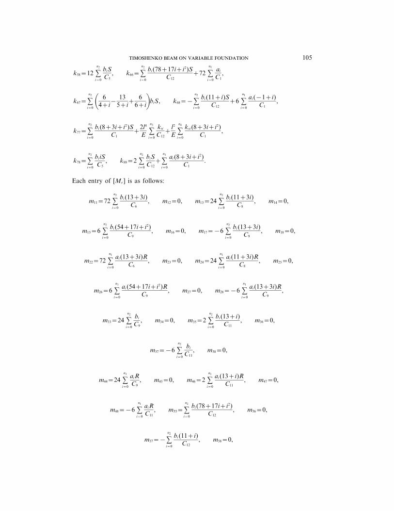
Each entry of [Me ] is as follows:

m11=72 sn2

i=0

bi (13+3i)C6

, m12=0, m13=24 sn2

i=0

bi (11+3i)C8

, m14=0,

m15=6 sn2

i=0

bi (54+17i+i2)C9

, m16=0, m17=−6 sn2

i=0

bi (13+3i)C9

, m18=0,

m22=72 sn1

i=0

ai (13+3i)RC6

, m23=0, m24=24 sn1

i=0

ai (11+3i)RC8

, m25=0,

m26=6 sn1

i=0

ai (54+17i+i2)RC9

, m27=0, m28=−6 sn1

i=0

ai (13+3i)RC9

,

m33=24 sn2

i=0

bi

C9, m34=0, m35=2 s

n2

i=0

bi (13+i)C11

, m36=0,

m37=−6 sn2

i=0

bi

C11, m38=0,

m44=24 sn1

i=0

aiRC9

, m45=0, m46=2 sn1

i=0

ai (13+i)RC11

, m47=0,

m48=−6 sn1

i=0

aiRC11

, m55=sn2

i=0

bi (78+17i+i2)C12

, m56=0,

m57=−sn2

i=0

bi (11+i)C12

, m58=0,

. . .106

m66=sn1

i=0

ai (78+17i+i2)RC12

, m67=0, m68=−sn1

i=0

ai (11+i)RC12

,

m77=2 sn2

i=0

bi

C12m78=0, m88=2 s

n1

i=0

aiRC12

,

Here

C1=60+47i+12i2+i3, C2=720+1044i+580i2+155i3+20i4+i5,

C3=120+154i+71i2+14i3+i4, C4=360+342i+119i2+18i3+i4,

C5=120+74i+15i2+i3,

C6=2520+5274i+3929i2+1420i3+270i4+26i5+i6,

C7=240+508i+372i2+121i3+18i4+i5,

C8=5040+8028i+5104i2+1665i3+295i4+27i5+i6,

C9=2520+2754i+1175i2+245i3+25i4+i5,

C10=120+274i+225i2+85i3+15i4+i5,

C11=840+638i+179i2+22i3+i4,

C12=210+107i+18i2+i3, S=kGl2/E, R=1/l2.