A new estimate of the global 3D geostrophic ocean circulation based … · · 2014-03-27A new...

Deep-Sea Research II ] (]]]]) ]]]–]]]

Contents lists available at SciVerse ScienceDirect

Deep-Sea Research II

0967-06

http://d

n Corr

E-m

mrio@c

sguineh1 N

06230 V2 Al

d’Ocean

Pleasin-si

journal homepage: www.elsevier.com/locate/dsr2

A new estimate of the global 3D geostrophic ocean circulation based onsatellite data and in-situ measurements

S. Mulet a,n, M.-H. Rio a, A. Mignot a,1,2, S. Guinehut a, R. Morrow b

a CLS-Space Oceanography Division, 8-10 rue Herm�es, 31526 Ramonville St. Agne, Franceb LEGOS-OMP, 18 av. Edouard Belin, 31401 Toulouse Cedex 9, France

a r t i c l e i n f o

Keywords:

Geostrophic flow

Thermal wind equation

Meridional oceanic circulation

Observation based product

Remote sensing

Altimetry

45/$ - see front matter & 2012 Elsevier Ltd. A

x.doi.org/10.1016/j.dsr2.2012.04.012

esponding author. Tel.: þ33 5 61 39 37 36; fa

ail addresses: [email protected], sandrine.mulet@

ls.fr (M.-H. Rio), [email protected] (A. Migno

[email protected] (S. Guinehut), rosemary.morrow@le

ow at: CNRS, UMR 7093, Laboratoire d’Oce

illefranche-sur-Mer, France.

so at: Universite Pierre et Marie Curie-Pari

ographie de Villefranche, 06230 Villefranche

e cite this article as: Mulet, S., et al.tu measurements. Deep-Sea Res. II (

a b s t r a c t

A new estimate of the Global Ocean 3D geostrophic circulation from the surface down to 1500 m depth

(Surcouf3D) has been computed for the 1993–2008 period using an observation-based approach that

combines altimetry with temperature and salinity through the thermal wind equation. The validity of

this simple approach was tested using a consistent dataset from a model reanalysis. Away from the

boundary layers, errors are less than 10% in most places, which indicate that the thermal wind equation

is a robust approximation to reconstruct the 3D oceanic circulation in the ocean interior. The Surcouf3D

current field was validated in the Atlantic Ocean against in-situ observations. We considered the

ANDRO current velocities deduced at 1000 m depth from Argo float displacements as well as velocity

measurements at 26.51N from the RAPID-MOCHA current meter array. The Surcouf3D currents show

similar skill to the 3D velocities from the GLORYS Mercator Ocean reanalysis in reproducing the

amplitude and variability of the ANDRO currents. In the upper 1000 m, high correlations are also found

with in-situ velocities measured by the RAPID-MOCHA current meters. The Surcouf3D current field was

then used to compute estimates of the Atlantic Meridional Overturning Circulation (AMOC) through the

251N section, showing good comparisons with hydrographic sections from 1998 and 2004. Monthly

averaged AMOC time series are also consistent with the RAPID-MOCHA array and with the GLORYS

Mercator Ocean reanalysis over the April 2004–September 2007 period. Finally a 15 years long time

series of monthly estimates of the AMOC was computed. The AMOC strength has a mean value of 16 Sv

with an annual (resp. monthly) standard deviation of 2.4 Sv (resp. 7.1 Sv) over the 1993–2008 period.

The time series, characterized by a strong variability, shows no significant trend.

& 2012 Elsevier Ltd. All rights reserved.

1. Introduction

The accurate measurement of the ocean 3D circulation is a keyissue for a number of scientific challenges, including monitoring theMeridional Overturning Circulation, or calculating ocean heat trans-ports. General circulation models provide 3D current velocities onregional or global scales. They are a precious tool to carry out in-depth studies of the different ocean mechanisms, such as theMeridional Overturning Circulation (Cabanes et al., 2008). For manyocean applications, model reanalysis is needed to provide homo-geneous, long-term time series. For instance, the SODA reanalysis

ll rights reserved.

x: þ33 5 61 39 37 82.

cls.fr (S. Mulet),

t),

gos.obs-mip.fr (R. Morrow).

anographie de Villefranche,

s 6, UMR 7093, Laboratoire

-sur-Mer, France.

, A new estimate of the glo2012), http://dx.doi.org/10.

(Carton et al., 2000a, 2000b) was used by Zheng and Giese (2009) tostudy the global ocean heat transport. Reanalysis projects require ahuge amount of work in reprocessing data series of the global, highresolution 3D ocean models. Moreover, their validation is stronglydependent on the existence of independent observed currents.

In-situ measurements of the ocean currents at depth areroutinely made at only a few specific locations and in the frame-work of specific national or international programs like RAPID-MOCHA (Cunningham et al., 2007). In synergy with satelliteobservations, which provide a global, repetitive view of thesurface ocean state, the Argo array was launched in 2004 withthe objective of providing a global, 31�31 array of in-situestimate of the ocean temperature and salinity from the surfacedown to 1500–2000 m. In order to take advantage of the numer-ous, high quality and complementary satellite and in-situ oceanicmeasurements, observation-based products have been developed(Larnicol et al., 2006; Willis et al., 2003; Willis and Fu, 2008;Willis, 2010) in which different observations are combined usingstatistics, optimal analysis or simple equations (but no numericalmodel). These observation-based products are a simpler alternative

bal 3D geostrophic ocean circulation based on satellite data and1016/j.dsr2.2012.04.012

www.elsevier.com/locate/dsr2

www.elsevier.com/locate/dsr2

dx.doi.org/<mac_doitxt/>10.1016/j.dsr2.2012.04.012



mailto:[email protected]










S. Mulet et al. / Deep-Sea Research II ] (]]]]) ]]]–]]]2

to data assimilation using numerical models and are very useful tovalidate the accuracy of the model simulations and the impact of itsdynamics. Two 3D observation-based products have been developedat CLS. The first product is a so called ‘‘synthetic’’ 3D thermohalinefield deduced from a statistical projection of altimetry and SeaSurface Temperature (SST), available from the surface down to1500 m (Guinehut et al., 2004, 2012). The second one is a new 3Doceanic geostrophic circulation field described in the present paper.

Flow in the ocean interior (away from the boundary layers) andaway from the equator is in geostrophic balance to the first order assuggested by observations and scaling arguments (Wunsch, 1996,chapter 2), even in boundary currents such as the Atlantic DeepWestern Boundary Current (Johns et al., 2005). In this paper, the 3Doceanic circulation is computed assuming geostrophic balance andusing the thermal wind equation, taking the reference level at thesurface where the geostrophic currents are well known and derivedfrom altimetric sea level heights. The horizontal density gradient inthe thermal wind equation is provided by the synthetic thermohalinefield mentioned above. Global weekly, monthly and yearly 3D oceaniccurrents from the surface down to 1500 m (hereafter called theSurcouf3D Currents) have been calculated from 1993 to 2008.

In the first part of this paper, we check the validity of theapproach by applying the thermal wind equation to a consistentoceanic data set from the GLORYS1V1 model reanalysis (Ferryet al., 2010; Lique et al., 2011). We then compare the Surcouf3Dcurrents to in-situ data in the Atlantic Ocean where there is astrong oceanic overturning circulation. It is also the mostobserved ocean which makes the validation easier. We validatethe weekly reanalysis at 1000 m depth through a comparisonwith in-situ velocities from Argo floats (Ollitrault et al., 2006;Ollitrault and Rannou, 2010) and modeled velocities from theGLORYS1V1 reanalysis. Comparisons are also made with theRAPID-MOCHA current meters located in the western boundarycurrent at 26.51N. In the last part of the paper, we use theSurcouf3D currents to estimate the Meridional Overturning Cir-culation (MOC). Two time series are computed. The first one, at251N, spans the 1993–2008 period and is compared to previousresults by Bryden et al. (2005) (referred as BR05 subsequently),calculated from full-depth hydrographic sections. The secondtime series, computed at 26.51N, spans the 2004–2007 periodand is compared with results from GLORYS1V1 reanalysis and theRAPID-MOCHA monitoring project. In both cases, monthly meansof the Surcouf3D currents are used in order to focus on theseasonal and interannual variability of the MOC.

The paper is organized as follows. After presenting the data inSection 2 and describing the computation method of the Sur-couf3D currents in Section 3, Section 4 is dedicated to thecomparisons with other existing products. The 1993–2008 and2004–2007 time series of the monthly estimated AMOC throughthe 251N and 26.51N sections are analyzed in Section 5. Discus-sion and conclusions are given in Section 6.

2. Data

Five types of data are used in this study. The first two types(altimetric measurements and the synthetic thermohaline field)are used in the computation of the 3D geostrophic velocitieswhile the three other ones (GLORYS reanalysis, estimates of Argofloat velocities and current meter measurements from the RAPID-MOCHA database) are used for validation purposes.

2.1. Gridded maps of surface altimetric geostrophic currents

We use weekly 1/31 resolution maps of delayed-time geos-trophic surface currents computed by the SSALTO/DUACS center

Please cite this article as: Mulet, S., et al., A new estimate of the gloin-situ measurements. Deep-Sea Res. II (2012), http://dx.doi.org/10.

and distributed by AVISO from January 1993 to December 2008(SSALTO/DUACS, 2011). The altimetric data used in the computa-tion of the multimission maps of Sea Level Anomaly (SLA) arefrom the ERS-1,2, ENVISAT, Topex/Poseidon, Jason-1,2, GFO,GEOSAT satellites. The CMDT RIO05 (Rio and Schaeffer, 2005)Mean Dynamic Topography (MDT) is added to the SLA maps toobtain maps of absolute dynamic topography, that are then usedto infer the ocean surface currents through geostrophy. Whencomputing absolute geostrophic currents from altimetry, thedominant error comes from the mean circulation. The determina-tion of this error is quite challenging. In Rio and Schaeffer (2005)the MDT is validated using a dataset of independent drifting buoymeasurements of the surface current velocities from which theEkman component is extracted. Altimetric geostrophic velocityanomalies are collocated to the in-situ data and the meangeostrophic currents derived from the RIO05 MDT are used toobtain absolute collocated geostrophic velocities. In the AtlanticOcean, the Root Mean Square difference between both geos-trophic velocity datasets (in-situ and altimetric) is in the orderof 12 cm/s for both components of the velocity. This value reducesto less than 9 cm/s away from strong Western Boundary Currents(Rio and Schaeffer, 2005). This RMS value is the sum of differenterror components (error on the Ekman model, error on thealtimetric velocity anomalies, error on the in-situ drifting buoymeasurements and error on the RIO05 MDT currents) so that it isan overestimate of the true RIO05 MDT error.

2.2. 3D synthetic thermohaline field

The weekly 3D synthetic thermohaline field is an observation-based product deduced from SLA and Sea Surface Temperature(SST) through a statistical projection as described by Guinehutet al. (2004, 2012). The altimeter data come from the SSALTO/DUACS center and are described in Section 2.1. The sea surfacetemperature fields are Reynolds 1/41 products (Reynolds et al.,2007).

The main idea of the method is to start from a smooth firstguess, the monthly ARIVO climatology based on Argo measure-ment (Gaillard and Charraudeau, 2008) and use high resolutionsatellite observations to improve it. First the baroclinic compo-nent (H) of the SLA due to the density variations from the surfaceto a chosen reference level is extracted using regression coeffi-cients deduced from an altimeter/in-situ comparison study. Theregression coefficients have been calculated using collocateddynamic height anomalies computed from Argo temperatureand salinity profiles and altimeter SLA (Dhomps et al., 2011;Guinehut et al., 2006). Using a reference level at 1500 m depth orat the bottom in coastal areas shallower than 1500 m, theregression coefficients range from 0.8 in the equatorial andtropical regions to 0.7 and 0.2 in mid to high latitudes with aclear latitudinal dependency. These values mean that most of thealtimeter SLA signal is projected onto the vertical ocean structureat low latitudes but that only 70–20% are projected at mid to highlatitudes, where the barotropic and deep baroclinic signals aremore important.

Secondly, a multiple linear regression method is used (Eq. (1))to provide temperature (T0) and salinity (S0) anomalies relative tothe monthly ARIVO climatology (Gaillard and Charraudeau, 2008):

T 0ðx,y,z,tÞ ¼ aðx,y,z,tÞH0ðx,y,tÞþbðx,y,z,tÞSST 0ðx,y,tÞ

S0ðx,y,z,tÞ ¼ gðx,y,z,tÞH0ðx,y,tÞ ð1Þ

Here H0 and SST0 are anomalies of the baroclinic height and seasurface temperature, respectively, relative to the monthly ARIVOclimatology. The regression coefficients a, b and g have spatial andseasonal dependency and are computed from historical in-situ T/Sprofiles (Argo floats, XBT, CTD) distributed by the ENACT and





290° 300° 310° 320° 330° 340° 350° 0° 10° 20°−70°

−60°

−50°

−40°

−30°

−20°

−10°

0°

10°

20°

30°

40°

50°

60°

70°

80°

0 2 4 6 8 10 12 14 16 18 20

cm/s

Fig. 1. Mean positions and intensities of the mean velocities (cm/s) of the Argo

floats from the ANDRO database over their 10-days-displacement at 1000 m depth

for the 2006–2007 period.

S. Mulet et al. / Deep-Sea Research II ] (]]]]) ]]]–]]] 3

Coriolis data centers from 1950 to 2008. They are calculated on a11�11 regular grid using the historical data available in 51latitude�101 longitude radius of influence around each grid point.

Finally, the ARIVO climatology is added back to the anomalies tocompute the synthetic thermohaline field. The heaviest computa-tional step is the evaluation of the regression coefficients. But oncethey are computed for each map of SLA and SST, it is easy tocompute thermohaline fields. These 3D fields are computed weeklyon a global 1/31 Mercator grid and on 24 Levitus levels from 0 to1500 m. The first levels to 30 m are spaced by 10 m, and then thespace increases to reach 100 m between 300 and 1500 m. The1500 m reference level was chosen in order to have enough in-situdata to compute statistically significant regression coefficients.Indeed, although many Argo floats descend to 2000 m depth, amajority of the historical floats descend only to 1500 m depth. Inaddition to the real-time production, reanalyses that use betterreprocessed observations (SLA, SST) are regularly generated. For thisstudy, we use a reanalysis of the synthetic thermohaline field thathas been computed recently and covers the 1993–2008 period.

The quality of the synthetic fields depends mainly on therelationship that exists between the surface and subsurfacefields. For example, the temperature field within the mixed layeris very well constrained by the SST field everywhere. Below themixed layer, mid to high latitudes are well constrained by theSLA with correlation greater than 0.7 between SLA and temperatureat depth. In the tropics, even though the correlation betweenSLA and temperature at depth is smaller and in the order of 0.4,the projection of mesoscale surface signal still allows us toadd information to the first guess (Guinehut et al., 2012). In theregression applied to salinity, only the SLA is used since global andhigh resolution fields of Sea Surface Salinity observations are notyet available. Improvements are indeed expected with the ongoingSMOS (Silvestrin et al., 2001) and Aquarius missions (Le Vine et al.,2007). Although the correlation between surface SLA and salinity atdepth is lower than that between SLA and temperature everywhere,the first guess is again improved by projecting the SLA at depth(Guinehut et al., 2012).

2.3. GLobal Ocean ReanalYses and Simulations (GLORYS) field

GLORYS is an ocean general circulation model reanalysisproduct based on a slightly modified version of the PSY3V2operational system from Mercator Ocean (Ferry et al., 2010;Lique et al., 2011). The configuration is global on a 1/41 ORCAgrid with 50 vertical levels. It assimilates SST maps, along trackSLA and in-situ T/S profiles, using the SEEK extended Kalmanfiltering assimilation technique. The mean dynamic topography(MDT) used to assimilate the SLA is the CMDT RIO05 product (Rioand Schaeffer, 2005) combined with a nearshore numerical model.

Here we use the weekly and monthly averaged 3D velocityfields from the first version of GLORYS (GLORYS1V1), availableover the time period 2002–2008.

2.4. Argo New Displacement Rannou Ollitrault (ANDRO) observed

velocity database

The nominal cycle of an Argo float is to dive down to itsparking depth where it drifts for about 10 days, before diving to2000 m and going back to the surface measuring T/S profiles. Onceat the surface the Argo float is located by satellite several timesduring a �12-hour period, where it drifts with the surfacecurrents. The Argo displacement at depth can thus be estimatedfrom the locations of the last float position observed by thesatellite at the sea surface before the float dives and of the firstone after the float comes back at the surface.


The ANDRO database (Ollitrault et al., 2006; Ollitrault andRannou, 2010) contains velocity displacements of the Argo floatsat their parking depths (1000 m mostly but also 1500 m and2000 m) from 2002 to 2007. ANDRO is only based on datadistributed by the AOML and Coriolis Data Assembly Centers.The Argo float displacement data have been corrected beforecomputing the drifting velocity. The main corrections concern theparking pressure and the surface positions determined by satellitelocalization. The error associated with this database is of order1 cm/s (Ollitrault et al., 2006; Ollitrault and Rannou, 2010).

In this paper we use the ANDRO velocity displacements at1000 m in the Atlantic Ocean for 2006 and 2007 that representmore than half of the entire ANDRO set (i.e. more than 13,000velocity estimates). Trajectories of the floats and their velocitiesare shown in Fig. 1. The ANDRO database, by construction,represents mean velocities over 10 days which are averaged overthe drift distance that occurred during these 10 days. The meandisplacement ranges from less than 50 km in the center of thesub-tropical gyres to 100–150 km in strong currents such as theGulf Stream or the Antarctic Circumpolar Current (Fig. 2).

2.5. RAPID-MOCHA array

RAPID-MOCHA is a joint program involving the U.K. RapidClimate Change (RAPID) program and the U.S. Meridional Over-turning Circulation and Heatflux Array (MOCHA) project. It con-sists of around twenty moorings equipped with CTDs andpressure sensors deployed at 26.51N at the western boundary,





290° 300° 310° 320° 330° 340° 350° 0° 10° 20°

0°

−70°

−60°

−50°

−40°

−30°

−20°

−10°

10°

20°

30°

40°

50°

60°

70°

80°

0 20 40 60 80 100 120 140 160 180 200mean displacement (km)

Fig. 2. Mean displacement (km) over 10 days of the Argo floats from the ANDRO

database at 1000 m depth from January 2006 to December 2007.


around the mid-Atlantic ridge and at the eastern boundary.Current meters have also been deployed at the western boundaryto resolve the western boundary currents (Johns et al., 2008). Inthis study, we used the monthly averaged velocities from thecurrent meters and T/S profiles at the western boundary deployedin March 2004 and recovered in May 2005.

We also use the monthly averaged Meridional OverturningCirculation (MOC) estimated from April 2004 to September 2007in the framework of the RAPID-MOCHA project as described by(Cunningham et al., 2007; Kanzow et al., 2007).

3. Method

The geostrophic components of the ocean circulation can becomputed at all depths zi using the thermal wind equation:

uðz¼ ziÞ ¼ uðz¼ 0Þ�g

rf

Z z ¼ 0

z ¼ zi

@

@yrðzÞ dz

vðz¼ ziÞ ¼ vðz¼ 0Þþg

rf

Z z ¼ 0

z ¼ zi

@

@xrðzÞ dz ð2Þ

The first terms on the right hand side of Eq. (2) are the velocitycomponents due to the sea surface slope current while the secondterms are the components of baroclinic velocity resulting fromhorizontal density gradients from the surface to z¼zi.

The geostrophic ocean currents at the surface u(z¼0), v(z¼0)are estimated from the altimetric maps of absolute dynamic


topography (computed as the sum of the SLA and the MDT). Thedensities at depth r(z) are computed from the synthetic thermo-haline field. We thus obtain weekly 3D grids of current velocitiesat the same horizontal and vertical resolution as the syntheticthermohaline field (global 1/31 Mercator grid on 24 Levitus levelsfrom the surface to 1500 m). Since the geostrophic approximationis not verified near the equator, no current is estimated in theequatorial band between 51S and 51N. Also, there is no estimationwhere the CMDT RIO05 (Rio and Schaeffer, 2005) or the SLA is notdefined, in semi-enclosed seas (Mediterranean, Black and Redseas) and high latitudes. In the following, we will refer to this 3Dvelocity estimate as Surcouf3D.

Classically, relative velocities are computed from T/S fields usingthe thermal wind equations assuming a level of no motion. Fig. 3(A)shows the 2006 annual mean velocities obtained from the syntheticthermohaline field and the thermal wind equation assuming a levelof no motion at 1500 m. The Surcouf3D currents are displayed inFig. 3(B). While the relative velocities to 1500 m only resolve, byconstruction, the baroclinic component of the circulation relative to1500 m, the Surcouf3D velocities contain both the shallower anddeeper baroclinic components and also the barotropic component ofthe ocean circulation. As a result, the relative velocities to 1500 mare weak compared to the Surcouf3D estimate; the Gulf Streamsignature (at 391N) shows a maximum velocity of around 35 cm/sand a maximum extension of 900 m (Fig. 3A). The Gulf Streamvelocity computed with Surcouf3D extends deeper and is clearlystronger (maximum velocities greater than 50 cm/s), in betteragreement with the GLORYS current estimate (Fig. 3C). The recircu-lation cells associated with the Gulf Stream in the Surcouf3D field arealso in much better agreement with GLORYS than the relativevelocities to 1500 m. Indeed, the westward current at 271N is betterresolved and the long-lived recirculation pattern centered around35.51N is modified with an intensification of the westward branchand a slowing down of the eastward branch. Also, north of the GulfStream, the Surcouf3D and the GLORYS currents are consistent, withan eastward current at 421N and a westward current which is deeperand shifted to the south. However, the Surcouf3D velocities arestronger than the GLORYS ones and contain more mesoscale varia-bility at depth. This is more clearly visible in Fig. 4 where the 2006annual mean horizontal currents at 500 m depth from Surcouf3Dand GLORYS are compared in the Gulf Stream region. Both of theSurcouf3D and GLORYS fields are based on the use of altimetry, SSTand T/S profiles, except GLORYS uses a full data assimilation scheme.Despite some small discrepancies, the two fields are in goodagreement, which is a very promising result for such a simplevelocity computation method as Surcouf3D.

In order to further assess the accuracy of the Surcouf3D andthe GLORYS velocity field we will compare them in the nextsection to independent data (the ANDRO dataset in Sections 4.2and the RAPID-MOCHA current meter array in Section 4.3).

4. Assessment of the Surcouf3D accuracy

4.1. Validity of the thermal wind equation

The assumption made to compute the Surcouf3D field is basedon the validity of the thermal wind relation to derive absolutehorizontal velocities. In this section, we test this assumptionthrough the use of an ocean model reanalysis GLORYS1V1 overthe 2006–2007 periods.

The temperature (T), salinity (S), height above geoid (H) andcurrent (Unat/Vnat) fields from the GLORYS daily reanalysis arefirst weekly averaged. Then the thermal wind equation is appliedusing the GLORYS T/S/H fields. The reference level is set at thesurface (Eq. (2)), where the velocities are computed from the





−1500

−1000

−500

0

0

0

0

−1500

−1000

−500

0

0

−1500

−1000

−500

0

−1500

−1000

−500

0

25°N 30°N 35°N 40°N

−20 −15 −10 −5 0 5 10 15 20 25 30 35 40 45 50(cm/s)

Fig. 3. Vertical structures of the 2006 annual mean zonal velocities (cm/s) along a section in the Gulf Stream at 601W (see black line in Fig. 4) for (A) the velocities relative

to 1500 m, (B) Surcouf3D, (C) GLORYS and (D) the geostrophic velocities computed from the H/T/S GLORYS fields through the thermal wind equation.


GLORYS H field using the geostrophic approximation. At eachvertical level, the geostrophic current field (Ugeo/Vgeo) is recon-structed by integrating the horizontal density gradients computedfrom the T/S fields, following Eq. (2). Finally we compared thereconstructed geostrophic current field (Ugeo/Vgeo) with thenative current field from GLORYS (Unat/Vnat).

Fig. 3(D) shows the 2006 yearly averaged geostrophic mer-idional velocities at 601W reconstructed from GLORYS H/T/Sfields. There are very few differences even in the surface layerscompared to Fig. 3(C) that shows the same profile for the nativeGLORYS current field. Thus, the ageostrophic components inGLORYS, including the surface Ekman currents, have very littleimpact on the annual mean in the Gulf Stream area. In the case of


weekly fields, larger differences are obtained near the surface,which are typical of the Ekman circulation (not shown).

Outside the Ekman layer, there is no bias between the recon-structed and the native weekly fields. At 600 m the absolute meandifferences are less than 0.1 cm/s both for the zonal and themeridional components. Figs. 5 and 6 show the standard deviationof the differences between the native and the reconstructed currents,computed in 201�201 boxes at different depths (Fig. 6) and bylatitudinal bands of 201 (Fig. 5). Values are expressed as a percentageof the standard deviation of the native field. In the first 50 m(Figs. 5 and 6A and B) the error is between 20% and 50%. This highsurface layer error is due to the Ekman currents which are includedin the native currents but not in the reconstructed, geostrophic field.





280° 290° 300° 310°20°

25°

30°

35°

40°

45°

280° 290° 300° 310°20°

25°

30°

35°

40°

45°

0 10 20 30 40 50 60 70(cm/s)

Fig. 4. Circulation in 2006 at 500 m depth in the Gulf Stream area from (A) Surcouf3D

estimate and (B) GLORYS reanalysis. The black line shows the section at 601W used in

Fig. 3.


Below the Ekman layer, the error is much smaller, less than 12% atdepths larger than 500 m (Fig. 5). At 200 m (Fig. 6C and D), in theocean interior, the error is lower than 10% everywhere, except in theNorth Atlantic gyre where the error is about 13%. Higher errors alsooccur closer to the coasts, probably due to other ageostrophicprocesses. This is the case for the very coastal Western BoundaryCurrents (East Australian Current, Florida Current), for certainupwelling currents system (Benguela Current, Canary Current) or incomplex bathymetric areas (China sea, Gulf of Mexico). However theerrors remain less than 20%.

To conclude, we find that with a weekly temporal resolutionand a 1/31 grid, the thermal wind equation is a robust approx-imation to reconstruct the 3D ocean velocity field in the oceaninterior with errors lower than 10% in most places. Close to thecoasts, where friction becomes non negligible, the error is higher,up to 20%. Errors up to 50% are found near the surface, where theageostrophic Ekman currents are a significant contribution to thetotal current.


4.2. Comparison to the ANDRO velocity database

We interpolated the observation-based currents (both theSurcouf3D currents and the velocity field relative to 1500 m)and the modeled currents (GLORYS) onto the date and position ofthe Argo floats drifting at 1000 m in the Atlantic between 2006and 2007 (see Fig. 1). Then, for each field, a statistical comparisonwas made with the in-situ Argo float velocities. Results are verysimilar for the zonal and meridional components (Table 1). In thefollowing, we will only discuss the meridional component, whichis weaker and more difficult to estimate accurately.

There is no bias between the Surcouf3D (resp. GLORYS) andANDRO meridional velocities with a mean difference of 0.35 cm/s(resp. 0.5 cm/s). The amplitudes of the variability of the Sur-couf3D and GLORYS meridional components are also very close(standard deviations are respectively 6.92 and 6.95 cm/s) butboth are higher than the in-situ observations (5.70 cm/s). This ismainly due to the Argo sampling frequency. The mean displace-ment of the Argo float in 10 days (Fig. 2) is around 50 km in thewhole Atlantic and more than 100 km in region of high variability(south of the southern subtropical gyre, Gulf Stream area) whilethe resolution of Surcouf3D and GLORYS is 1/31 and 1/41 respec-tively. Note that while the temporal averaging is consistentbetween the different data sets, the Argo float velocity is a 10days lagrangian average estimate whereas the Surcouf3D andGLORYS are representative of eulerian weekly mean fields.Meijers et al. (2011) have quantified the error between this typeof lagrangian and eulerian fields to be around 3.9 cm/s nearKerguelen Island.

Both Surcouf3D and GLORYS show a correlation higher thanthe 99% significance level defined by Emery and Thomson (1998).Surcouf3D shows a good correlation with the Argo drift velocities(0.6) while GLORYS is less consistent (0.42). The standard devia-tion of the differences to Argo floats is smaller with Surcouf3D(5.75 cm/s) than with GLORYS (6.91 cm/s). The smallest differ-ence is obtained with the velocities calculated relative to 1500 m(5.13 cm/s). However, this relative velocity field fails to resolvethe variability of the ocean circulation (the standard deviation is1.23 cm/s, to be compared with 5.7 cm/s for the Argo floats). Inorder to have a synthetic vision of these different statistics, weuse the skill score (STaylor) defined by Taylor (2001) and given bythe following equation:

STaylor ¼ 2ð1þRÞ

ððsr=sf Þþðsf =srÞÞ2

ð3Þ

where R is the correlation coefficient between the two fields f andr that are compared, sf and sr are their standard deviations. Thescore varies from zero to one. The score approaches one if the twofields that are compared are correlated and have similar varia-bility. The highest skill is obtained with Surcouf3D (0.77) followedby GLORYS (0.68). The relative velocity field is highly penalized(0.14) because it contains very low signal at 1000 m, with muchweaker horizontal density gradients here (see also Fig. 3).

4.3. Comparison to the RAPID current meter velocities

Velocities at various depths has been routinely measured fromApril 2004 in the western boundary current off the Bahamas(26.51N, 76.51W) by current meters from the RAPID-MOCHAproject (Johns et al., 2008). In this study we consider the timesseries from April 2004 to October 2006. The Surcouf3D monthlyvelocities, interpolated onto the current meter locations (Fig. 7),show a very good consistency with the current meter velocitiesover the first 400 m, with a correlation coefficient up to 0.96 atthe 99% significance level. For the GLORYS dataset, the correlationcoefficient is 0.82. The correlation coefficient decreases with





Fig. 5. Standard deviation (%) of the differences between the GLORYS native and the reconstructed currents computed by latitudinal bands of 201 and at different depths

for (A) the zonal component and (B) the meridional component. Values are expressed as a percentage of the standard deviation of the native field.


depth but the Surcouf3D and RAPID-MOCHA zonal velocitiesremain correlated. At 800 m, the correlation coefficient is 0.68at the 99% confidence level and at 1200, where the zonal flow isweak, it is 0.41 at the 95% confidence level.

The RAPID-MOCHA meridional current is directed northwardat depths shallower than 800 m, and southward at 1200 m,except for November 2004 when a maximum of northwardmeridional velocity extends from 100 m to 1200 m and forJanuary 2006. The vertical shear of the meridional current isresolved by the GLORYS currents, but not by the Surcouf3D field.This may be due to the predominance of ageostrophic dynamics,not taken into account by our simple, geostrophic methodology.However, Fig. 6 shows that ageostrophic processes in this areacontribute only to 13% of the signal at depth. This is in goodagreement with Johns et al. (2005) mentioning that this currentis mainly in geostrophical balance. To further check the validityof applying the thermal wind equation to resolve this strongcurrent shear, we have applied our methodology using two T/Sprofiles from the RAPID-MOCHA array (at 76.501W and 76.751W)


and using as reference velocities values the current meter locatedat 100 m depth at 76.51W. The obtained currents (dotted redlines in Fig. 7) correctly resolve the inversion of the meridionalcomponent around 800 m (Johns et al., 2008). The failure of theSurcouf3D field to resolve the meridional current shear is there-fore not due to the geostrophic approximation, but rather to thefailure of the synthetic thermohaline field to capture the strongdensity shear associated with this narrow current system. In thefuture, we plan to improve the thermohaline field by combiningit with Argo float profiles in order to improve locally thedescription of the ocean 3D T/S characteristics. Note that thegeostrophic meridional velocity profile computed from theRAPID-MOCHA T/S profiles does not match exactly the currentmeter measurements (dotted and solid red lines in Fig. 7). This ismainly because these fields do not represent the current at thesame location. The current meters give measurements at 76.51Wwhile the geostrophic meriodional velocity profile is evaluatedbetween the location of the two T/S profiles (76.51W and76.751W).





Fig. 6. Standard deviation (%) of the differences between the GLORYS native and the reconstructed currents computed in 201�201 boxes (A, B) at 10 m, (C, D) at 200 m and

(E, F) at 600 m for (left) the zonal component and (right) the meridional component. Values are expressed in percentage of the standard deviation of the native field.

Table 1Results of statistical comparisons of three current fields (Surcouf3D, GLORYS and velocities relative to 1500 m) to Argo floats drifting at 1000 m in the Atlantic over 2006/

2007 period.

Surcouf3D GLORYS Velocities relative to 1500 m Argo floats (ANDRO database)

Velocity components (U: zonal, V: meridional) U V U V U V U V

Standard deviation (cm/s) 7.27 6.92 7.23 6.95 1.31 1.23 5.97 5.70

Correlation coefficient 0.61 0.60 0.46 0.42 0.58 0.55

Standard deviation of the differences (cm/s) 5.93 5.75 6.93 6.91 5.32 5.13

Mean difference (cm/s) �0.22 0.35 0.10 0.50 �0.18 0.13

Taylor’s score 0.78 0.77 0.71 0.68 0.14 0.14


5. Application: monitoring the Atlantic Meridional OceanicCirculation (AMOC)

According to Kanzow et al. (2007), overturning at 251N in theAtlantic can be divided into three components: the Floridawestern boundary transport, the surface Ekman transport and


the interior geostrophic transports, the last two being integratedfrom the Bahamas to Africa. In the traditional approach, only thebaroclinic part of the geostrophic transport relative to a referencelevel is computed, which is why a time variant offset must beadded to impose mass conservation. Kanzow et al. (2006) usesbottom pressure sensors to overcome this issue. These sensors





Fig. 7. April 2004–2005 time series of the monthly mean (A) zonal and (B) meridional velocities interpolated at the localization of the current meters from RAPID-MOCHA

in the western boundary current off the Bahamas. In black dashes: Surcouf3D, in blue dashes and dots: GLORYS, in solid red lines: current meters from RAPID-MOCHA at

76.51W, and red dots: current computed through the thermal wind equation using T/S profiles and current meter at 100 m from RAPID-MOCHA. The correlation coefficients

with RAPID-MOCHA measurements are written in the top right of each panel, Rs refer to correlation with Surcouf3D time series and Rg to the GLORYS time series. (For

interpretation of the references to color in this figure legend, the reader is referred to the web version of this article.)


cannot measure the absolute pressure with sufficient accuracybut do give access to the bottom pressure fluctuations and thus tothe transport relative to the time mean value (Kanzow et al.2006). While the transport variability can be studied withoutmaking any further assumptions, a time invariant offset must beadded to assess absolute transport (Kanzow et al., 2007). Incontrast, the Surcouf3D product is an estimate of the absolutegeostrophic velocities at any level from the surface to 1500 m, sothe total transport at 251N in the 1500 first meters can betheoretically derived from the summation of its three compo-nents (the geostrophic component evaluated from Surcouf3D andthe Ekman and Florida current components) without adding anyoffset. However, errors inherent in the Surcouf3D fields, onceintegrated over the section, can break the mass balance. Forinstance, the transport is very sensitive to an error in the east–west MDT gradient. The limited vertical extension of the Sur-couf3D field also prevents us from imposing mass conservationover the water column through an offset computation. Despitethis difficulty, there is good agreement with other AMOC esti-mates (shown in the following) which gives us confidence in therobustness of the Surcouf3D fields.

A quantity commonly used to study overturning is its max-imum value at depth that is reached at around 1000 m at 251N(BR05; Hirschi et al., 2003). In the following we thus study thetransport integrated from the surface to 1000 m. We first


compute the meridional geostrophic transport integrated fromthe surface to 1000 m and from the Bahamas to Africa (uppermid-ocean geostrophic transport) using the Surcouf3D velocityfield (blue circles in Fig. 8). The upper mid-ocean geostrophictransport was found to be significantly dependant on the chosenlatitude, mainly due to the differences in circulation in thewestern part of the section as BR05 already pointed out. Forinstance the upper mid-ocean geostrophic transport in 2004 is�17.1 Sv at 24.51N while it is �21.3 Sv if computed though theexact BR05 section (section at 24.51N angled northwestward at731W to finish along 26.51N to the Bahamas) including 2 Sv fromthe flow through the northwest Providence channel (BR05;Leaman et al., 1995). In Fig. 8, the different components of themaximum AMOC strength have therefore been computed alongthe exact BR05 section to allow for a rigorous comparison.

The Florida current transport (red stars in Fig. 8) is obtainedfrom the cable measurements that have been performed dailyfrom 1982 (Larsen, 1992). The meridional Ekman transport (greensquares in Fig. 8) is computed using the 80 km resolution windstress maps from the ERA INTERIM reanalysis (Simmons et al.,2007). Finally the maximum AMOC strength time series (blacktriangles in Fig. 8) is inferred by adding the three previouscomponents for each month from 1993 to 2008.

The upper mid-ocean geostrophic transport and thus theAMOC strength time series are characterized by a strong





0

5

−40

−35

−30

−25

−20

−15

−10

−5

10

15

20

25

30

35

40

Tran

spor

t (S

v)

1992 1993 1994 1995 1996 1997 1998 1999 2000 2001 2002 2003 2004 2005 2006 2007 2008

Florida Straits Transport AMOC Ekman Transport Upper Mid−Ocean Geostrophic Transport

Fig. 8. Monthly (thin lines) and yearly (thick lines) time series of the Florida Strait Transport (red stars), Ekman Transport (green squares), upper mid-ocean geostrophic

Transport computed from Surcouf3D (blue circles) and AMOC maximum strength (black triangles) through the BR05 section at 251N for the 1993–2008 period. Red

inverted triangles represent results from BR05 with the associated error bars. The gap from November 1998 to May 2000 is due to a gap in the Florida transport estimate.

(For interpretation of the references to color in this figure legend, the reader is referred to the web version of this article.)


variability at both seasonal to interannual time scales. The AMOCstrength has a mean value of 16 Sv with a full period yearlystandard deviation of 2.4 Sv, while the monthly standard devia-tion is 7.1 Sv. In spite of this high variability, our method givesvalues close to the BR05 ones and within the BR05 error interval(red inverted triangles and error bars on Fig. 8): we find an annualmean AMOC intensity of 17.49 Sv compared to 16.1 Sv in 1998and of 13.96 Sv compared to 14.8 Sv in 2004 (black triangles andred inverted triangles in Fig. 8). However, while BR05 suggested aslow down of 30%, the complete time series computed withSurcouf3D does not show any clear trend and is dominated by ahigh seasonal to interannual variability.


We then have compared our results to the values obtainedfrom the GLORYS reanalysis and the RAPID-MOCHA array overApril 2004 to September 2007 (Fig. 9). To be consistent with theAMOC time series estimated from the RAPID-MOCHA array, wehave computed the maximum AMOC strength across the samesection which starts at about 26.51N at the western boundary andends at about 27.51N at the eastern boundary. Good agreement isobtained for seasonal cycles (thick lines in Fig. 9) computed withthe three different datasets with a minimum in spring and amaximum in autumn. In 2004 the maximum in the Surcouf3Dtime series occurs slightly later than in the other time series. Thisis due to an overestimation of the Surcouf3D transport in





5

10

15

20

25

30

35

Tran

spor

t (S

v)

April 04 April 05 April 06 April 07

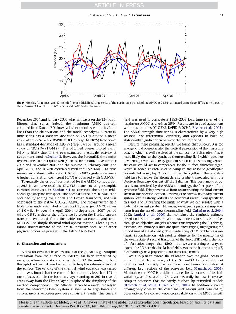
Fig. 9. Monthly (thin lines) and 12-month-filtered (thick lines) time series of the maximum strength of the AMOC at 26.51N estimated using three different methods. In

black: Surcouf3D, in blue: GLORYS and in red: RAPID-MOCHA array.


December 2004 and January 2005 which impacts on the 12-monthfiltered time series. Indeed, the maximum AMOC strengthobtained from Surcouf3D shows a higher monthly variability (thinline) than the observations and the model reanalysis. Surcouf3Dtime series has a standard deviation of 5.59 Sv around a meanvalue of 19.27 Sv while RAPID-MOCHA (resp. GLORYS) time serieshas a standard deviation of 3.95 Sv (resp. 3.61 Sv) around a meanvalue of 18.48 Sv (17.44 Sv). The obtained overestimated varia-bility is likely due to the overestimated mesoscale activity atdepth mentioned in Section 3. However, the Surcouf3D time seriesresolves the extrema quite well (such as the maxima in September2004 and November 2005 and the minima in February 2005 andApril 2007) and is well correlated with the RAPID-MOCHA timeseries (correlation coefficient of 0.67 at the 99% significance level).A higher correlation coefficient (0.77) is obtained with GLORYS.

To quantify the error of our method for the AMOC computationat 26.51N, we have used the GLORYS reconstructed geostrophiccurrents computed in Section 4.1 to compute the upper mid-ocean geostrophic transport. The reconstructed AMOC was thenobtained by adding the Florida and Ekman transports, and wascompared to the native GLORYS AMOC. The reconstructed fieldleads to an underestimated of the monthly averaged AMOC valuesof 1.670.4 Sv over the April 2004 to September 2007 periodwhere 0.9 Sv is due to the difference between the Florida currenttransport estimated from the cable measurements and fromGLORYS. The simple thermal wind approximation is leading to aminor underestimate of the AMOC, possibly because of otherphysical processes present in the full GLORYS field.

6. Discussion and conclusions

A new observation-based estimate of the global 3D geostrophiccirculation from the surface to 1500 m has been computed bymerging altimetric data and a synthetic 3D thermohaline fieldthrough the thermal wind equation setting the reference level atthe surface. The validity of the thermal wind equation was testedand it was found that the error of the method is less than 10% inmost places outside the boundary layers and up to 20% in coastalareas away from the Ekman layer. In spite of the simplicity of themethod, comparisons in the Atlantic Ocean to a model reanalysisfrom the Mercator Ocean system as well as to Argo floats andcurrent meters velocities give very consistent results. This current


field was used to compute a 1993–2008 long time series of themaximum AMOC strength at 251N. Results are in good agreementwith other studies (GLORYS, RAPID-MOCHA, Bryden et al., 2005).The AMOC strength time series is characterized by a very highseasonal and interannual variability and appears to have nostatistically significant trend over the entire period.

Despite these promising results, we found that Surcouf3D is tooenergetic and overestimates the vertical penetration of the mesoscaleactivity which is well resolved at the surface from altimetry. This ismost likely due to the synthetic thermohaline field which does nothave enough vertical density gradient structure. This missing verticalstructure would act to compensate for the surface altimetric signalwhich is added at each level to compute the absolute geostrophiccurrents following Eq. 2. For instance, the synthetic thermohalinefield fails to resolve the strong density gradient associated with theWestern Boundary Current off the Bahamas. This permanent struc-ture is not resolved by the ARIVO climatology, the first guess of thesynthetic field. This prevents us from reconstructing the local currentshear at this specific location. Resolving the narrow boundary currentsystem with its strong vertical and horizontal shear is very specific tothis area and is pushing the limits of what we can resolve with aglobal 3D current product. However, we expect significant improve-ment from the use of a new thermohaline field (Guinehut et al., 2004,2012; Larnicol et al., 2006) that combines the synthetic estimatebased on historical statistics with instantaneous in-situ T/S profilesthrough an objective analysis scheme, thus improving the 3D densityestimate. Preliminary results are quite encouraging, highlighting theimportance of a sustained global in-situ array of T/S profile measure-ments in combination with satellite altimetry for the monitoring ofthe ocean state. A second limitation of the Surcouf3D field is the lackof information deeper than 1500 m but we are working on ways toextend the 3D oceanic circulation field down to the bottom using a T/S climatology or a projection onto baroclinic modes.

We also plan to extend the validation over the global ocean inorder to test the accuracy of the Surcouf3D fields at differentlocations and to study the meridional overturning circulation atdifferent key sections of the conveyor belt (Ganachaud, 2003).Monitoring the MOC is a delicate issue, firstly because of its highvariability, as illustrated at 251N, and secondly because it involvescomplex processes that are barely resolved by numerical models(Biastoch et al., 2008; Hirschi et al., 2003). In addition, currentsflowing very close to the coast are not always well resolved byobservations. As a consequence, cross validation of the MOC strength






is essential (von Schuckmann et al., 2010). We are confident that thecomparison of this new 3D current field with other existing studiesbased on observations, or numerical models, will help better under-stand and monitor this key quantity of the climate system.

Acknowledgments

The authors would like to express their thanks to MichelOllitrault and Jean-Philippe Rannou for providing their ANDROatlas. They also would like to thanks the RAPID-MOCHA team forproviding data from the array. Data from the RAPID-WATCH MOCmonitoring project are funded by the Natural EnvironmentResearch Council and are freely available from www.noc.soton.ac.uk/rapidmoc. The realization of GLORYS1 global ocean reana-lysis had the benefit of the Grants that Groupe Mission MercatorCoriolis, Mercator-Ocean, and CNRS/INSU attributed to theGLORYS project, and the support of the European Union FP7 viathe MYOCEAN project. The altimeter products were produced bySsalto/Duacs and distributed by Aviso with support from CNES.The Florida Current cable and section data are made freelyavailable on the Atlantic Oceanographic and MeteorologicalLaboratory web page (www.aoml.noaa.gov/phod/floridacurrent/)and are funded by the NOAA Office of Climate Observations.Helpful comments from E. Greiner, N. Ferry and the reviewerswere appreciated.

References

Biastoch, A., Boning, C.W., Getzlaff, J., Molines, J., Madec, G., 2008. Causes ofinterannual–decadal variability in the meridional overturning circulation ofthe midlatitude North Atlantic Ocean. J. Climate 21, 6599–6615.

Bryden, H.L., Longworth, H.R., Cunningham, S.A., 2005. Slowing of the Atlanticmeridional overturning circulation at 251N. Nature 438 (7068), 655–657, http://dx.doi.org/10.1038/nature04385.

Cabanes, C., Lee, T., Fu, L.-L., 2008. Mechanisms of interannual variations of themeridional overturning circulation of the North Atlantic Ocean. J. Phys.Oceanogr. 38 (2), http://dx.doi.org/10.1175/2007JPO3726.1.

Carton, J.A., Chepurin, G., Cao, X., Giese, B.S., 2000a. A Simple Ocean DataAssimilation analysis of the global upper ocean 1950–1995, Part 1: methodol-ogy. J. Phys. Oceanogr. 30, 294–309.

Carton, J.A., Chepurin, G., Cao, X., 2000b. A Simple Ocean Data Assimilationanalysis of the global upper ocean 1950–1995 Part 2: results. J. Phys.Oceanogr. 30, 311–326.

Cunningham, S.A., Kanzow, T., Rayner, D., Baringer, M.O., Johns, W.E., Marotzke, J.,Longworth, R., Grant, E.M., Hirschi, J.J.-M., Beal, L.M., Meinen, C.S., Bryden, H.L.,2007. Temporal variability of the Atlantic meridional overturning circulationat 26.51N. Science 317 (5840), 935–938, http://dx.doi.org/10.1126/science.1141304.

Dhomps, A.-L., Guinehut, S., Le Traon, P.-Y., Larnicol, G., 2011. A global comparisonof Argo and satellite altimetry observations. Ocean Sci. 7, 175–183.

Emery, W.J., Thomson, R.E., 1998. Data Analysis Methods in Physical Oceanogra-phy. Pergamon (634 pp.).

Ferry, N., Parent, L., Garric, G., Barnier, B., Jourdain, N.C., the Mercator Ocean team,2010. Mercator Global Eddy Permitting Ocean Reanalysis GLORYS1V1:Description and Results. Mercator Ocean Quarterly Newsletter #36, January2010, pp. 15–27.

Gaillard, F., Charraudeau, R., 2008. New Climatology and Statistics Over the GlobalOcean. MERSEA-WP05-CNRS-STR-001-1A.

Ganachaud, A., 2003. Large-scale mass transports, water mass formation, anddiffusivities estimated from World Ocean Circulation Experiment (WOCE)hydrographic data. J. Geophys. Res. 108 (C7), 3213, http://dx.doi.org/10.1029/2002JC001565.

Guinehut, S., Le Traon, P.Y., Larnicol, G., Philipps, S., 2004. Combining Argo andremote-sensing data to estimate the ocean three-dimensional temperaturefields—a first approach based on simulated observations. J. Mar. Syst. 46 (1–4),85–98, http://dx.doi.org/10.1016/j.jmarsys.2003.11.022.

Guinehut, S., Le Traon, P., Larnicol, G., 2006. What can we learn from globalaltimetry/hydrography comparisons? Geophys. Res. Lett, 33, http://dx.doi.org/10.1029/2005GL025551.

Guinehut, S., Dhomps, A.-L., Larnicol, G., LeTraon, P.-Y., 2012. High resolution 3-Dtemperature and salinity fields derived from in situ and satellite observations.Ocean Sci. Discuss. 9, 1313–1347, http://dx.doi.org/10.5194/osd-9-1313-2012.


Hirschi, J., Baehr, J., Marotzke, J., Stark, J., Cunningham, S.A., Beismann, J., 2003. Amonitoring design for the Atlantic meridional overturning circulation. Geo-phys. Res. Lett. 30 (7), 1413, http://dx.doi.org/10.1029/2002GL016776.

Johns, W.E., Beal, L.M., Baringer, M.O., Molina, J.R., Cunningham, S.A., Kanzow, T.,Rayner, D., 2008. Variability of shallow and deep Western Boundary Currentsoff the Bahamas during 2004–05: results from the 261N RAPID–MOC array.J. Phys. Oceanogr. 38, 605–623, http://dx.doi.org/10.1175/2007JPO3791.1.

Johns, W.E., Kanzow, T., Zantopp, R., 2005. Estimating ocean transports withdynamic height moorings: an application in the Atlantic Deep WesternBoundary Current at 261N. Deep-Sea Res. I 52 (8), 1542–1567, http://dx.doi.org/10.1016/j.dsr.2005.02.002.

Kanzow, T., Send, U., Zenk, W., Chave, A., Rhein, M., 2006. Monitoring theintegrated deep meridional flow in the tropical North Atlantic: long-termperformance of a geostrophic array. Deep-Sea Res. I 53 (3), 528–546, http://dx.doi.org/10.1016/j.dsr.2005.12.007.

Kanzow, T., Cunningham, S.A., Rayner, D., Hirschi, J.J., Johns, W.E., Baringer, M.O.,Bryden, H.L., Beal, L.M., Meinen, C.S., Marotzke, J., 2007. Observed flowcompensation associated with the MOC at 26.51N in the Atlantic. Science317 (5840), 938–941, http://dx.doi.org/10.1126/science.1141293.

Larnicol, G., Guinehut, S., Rio, M.H., Drevillon, M., Faugere, Y., Nicolas, G., 2006. TheGlobal observed ocean products of the French Mercator project. In: Proceed-ings of the Symposium on 15 Years of Progress in Radar Altimetry 13–18March 2006, Venice, Italy.

Larsen, J.C., 1992. Transport and heat flux of the Florida Current at 271N derivedfrom cross-stream voltages and profiling data: theory and observations. Philos.Trans. R. Soc. London A 338, 169–236.

Le Vine, D.M., Lagerloef, G.S.E., Colomb, F.R., Yueh, S.H., Pellerano, F.A., 2007.Aquarius: an instrument to monitor sea surface salinity from space. IEEETrans. Geosci. Remote Sensing.

Leaman, K.D., Vertes, P.S., Atkinson, L.P., Lee, T.N., Hamilton, P., Waddell, E., 1995.Transport, potential vorticity, and current/temperature structure acrossNorthwest Providence and Santaren Channels and the Florida Current offCay Sal Bank. J. Geophys. Res. 100 (C5), 8561–8569.

Lique, C., Garric, G., Treguier, A., Barnier, B., Ferry, N., Testut, C., Girard-Ardhuin, F.,2011. Evolution of the Arctic Ocean salinity, 2007–08: contrast between theCanadian and the Eurasian Basins. J. Climate 24 (6), 1705–1717, http://dx.doi.org/10.1175/2010JCLI3762.1.

Meijers, A.J.S., Bindoff, N.L., Rintoul, S.R., 2011. Estimating the four-dimensionalstructure of the Southern Ocean using satellite altimetry. J. Atmos. OceanicTechnol.

Ollitrault, M., Lankhorst, M., Fratantoni, D., Richardson, P., Zenk, W., 2006. Zonalintermediate currents in the equatorial Atlantic Ocean. Geophys. Res. Lett. 33,L05605, http://dx.doi.org/10.1029/2005GL025368.

Ollitrault, M., Rannou, J.P., 2010. ANDRO: An Argo-based Deep Displacement Atlas.Mercator Ocean Quarterly Newsletter #37, April 2010, pp. 27–34.

Reynolds, R.W., Smith, T.M., Liu, C., Chelton, D.B., Casey, K.S., Schlax, M.G., 2007.Daily high-resolution-blended analyses for sea surface temperature. J. Climate20, 5473–5496, http://dx.doi.org/10.1175/2007JCLI1824.1.

Rio, M.-H., Schaeffer, P., 2005. The estimation of the ocean mean dynamictopography through the combination of altimetric data, in-situ measurementand GRACE geoid. In: Proceedings of the GOCINA International Workshop,Luxembourg.

von Schuckmann, K., Drevillon, M., Ferry, N., Mulet, S., Rio, M.-H., 2010. GlobalOcean Indicators. Mercator Ocean Quarterly Newsletter #37, April 2010, pp.20–28.

Silvestrin, P., Berger, M., Kerr, Y., Fontin, J., 2001. ESA’s second earth exploreropportunity mission: the soil moisture and ocean salinity mission-SMOS. IEEEGeosci. Remote Sensing Newsl.

Simmons, A., Uppala, S., Dee, D., Kobayashi, S., 2007. ERA-Interim: new ECMWFreanalysis products from 1989 onwards. ECMWF Newsl. 110, 25–35.

SSALTO/DUACS, 2011. User Handbook: MSLA and MADT Near-Real Time andDelayed Products. C.L.S., Ramonville St. Agne, France.

Taylor, K.E., 2001. Summarizing multiple aspects of model performance in a singlediagram. J. Geophys. Res. 106 (D7), 7183–7192.

Willis, J.K., Roemmich, D., Cornuelle, B., 2003. Combining altimetric height withbroadscale profile data to estimate steric height, heat storage, subsurfacetemperature, and sea-surface temperature variability. J. Geophys. Res. 108(C9), 3292, http://dx.doi.org/10.1029/2002JC001755.

Willis, J.K., Fu, L.-L., 2008. Combining altimeter and subsurface float data toestimate the time-averaged circulation in the upper ocean. J. Geophys. Res.113, C12017, http://dx.doi.org/10.1029/2007JC004690.

Willis, J.K., 2010. Can in situ floats and satellite altimeters detect long termchanges in Atlantic Ocean overturning? Geophys. Res. Lett. 37, L06602, http://dx.doi.org/10.1029/2010GL042372.

Wunsch, C., 1996. The Ocean Circulation Inverse Problem. Cambridge UniversityPress.

Zheng, Y., Giese, B.S., 2009. Ocean heat transport in Simple Ocean Data Assimilation:STructure and mechanisms. J. Geophys. Res. 114, C11009, http://dx.doi.org/10.1029/2008JC005190.


www.noc.soton.ac.uk/rapidmoc





www.aoml.noaa.gov/phod/floridacurrent/




dx.doi.org/<mac_doitxt/>10.1038/nature04385




dx.doi.org/<mac_doitxt/>10.1175/2007JPO3726.1



dx.doi.org/<mac_doitxt/>10.1126/science.1141304




dx.doi.org/<mac_doitxt/>10.1029/2002JC001565




dx.doi.org/<mac_doitxt/>10.1016/j.jmarsys.2003.11.022



dx.doi.org/<mac_doitxt/>10.1029/2005GL025551




dx.doi.org/doi:10.5194/osd-9-1313-2012

dx.doi.org/doi:10.5194/osd-9-1313-2012

dx.doi.org/doi:10.5194/osd-9-1313-2012







dx.doi.org/<mac_doitxt/>10.1016/j.dsr.2005.02.002











dx.doi.org/<mac_doitxt/>10.1175/2010JCLI3762.1



























A new estimate of the global 3D geostrophic ocean circulation based … · · 2014-03-27A new...

Documents

Transcript of A new estimate of the global 3D geostrophic ocean circulation based … · · 2014-03-27A new...