A New Efficient Stiffness Evaluation Method to Improve ...

HAL Id: hal-02025724https://hal.archives-ouvertes.fr/hal-02025724

Submitted on 2 Mar 2021

HAL is a multi-disciplinary open accessarchive for the deposit and dissemination of sci-entific research documents, whether they are pub-lished or not. The documents may come fromteaching and research institutions in France orabroad, or from public or private research centers.

L’archive ouverte pluridisciplinaire HAL, estdestinée au dépôt et à la diffusion de documentsscientifiques de niveau recherche, publiés ou non,émanant des établissements d’enseignement et derecherche français ou étrangers, des laboratoirespublics ou privés.

A New Efficient Stiffness Evaluation Method to ImproveAccuracy of Hexapods

Vinayak Jagannathrao Kalas, Alain Vissiere, Thierry Roux, Olivier Company,Sébastien Krut, François Pierrot

To cite this version:Vinayak Jagannathrao Kalas, Alain Vissiere, Thierry Roux, Olivier Company, Sébastien Krut, etal.. A New Efficient Stiffness Evaluation Method to Improve Accuracy of Hexapods. Interna-tional Design Engineering Technical Conferences and Computers and Information in Engineering(IDETC/CIE 2018), Aug 2018, Quebec City, Canada. pp.V05AT07A045, �10.1115/DETC2018-85986�.�hal-02025724�

https://hal.archives-ouvertes.fr/hal-02025724

https://hal.archives-ouvertes.fr

Proceedings of the ASME 2018 International Design Engineering Technical Conferences &Computers and Information in Engineering Conference

IDETC/CIE 2018August 26- 29, 2018, Quebec City, Canada

DETC2018-85986

A NEW EFFICIENT STIFFNESS EVALUATION METHOD TO IMPROVE ACCURACYOF HEXAPODS

Vinayak J. Kalas∗Department of Robotics

LIRMM34090 Montpellier, France

Email:[email protected]

Alain VissiereDepartment of Robotics


Email: [email protected]

Thierry RouxSymetrie

10 Allee Charles Babbage, 30035 NımesFrance


Olivier CompanyDepartment of Robotics



Sebastien KrutDepartment of Robotics



Francois PierrotDepartment of Robotics



ABSTRACTStructural compliance of hexapod positioners limits their

positioning accuracy. Taking a step towards solving this prob-lem, this paper proposes a new efficient method to evaluate thestiffness of hexapods in order to predict and correct their posi-tioning error due to compliance. The proposed method can beused to predict the six degree of freedom deflection of the plat-form under load. This method uses a simple lumped stiffnessparameter model whose parameters can be estimated using theidentification technique presented in this paper. An experimen-tal study with micrometer level measurements performed on ahexapod based micro-positioning system is used to assess the ef-ficiency of the presented method.

INTRODUCTIONHexapods, also called Gough-Stewart platforms, are in-

creasingly used for applications demanding high accuracy sixdegree of freedom (DOF) positioning. Some general areas ofapplications include mirror positioning in telescopes [1], posi-

∗Address all correspondence to this author.

tioning components in synchrotrons [2] and research applicationsdemanding high accuracy positioning [3]. One of the biggest ad-vantages of hexapods is their high inherent stiffness [4]. Hence,in most applications, hexapod compliance doesn’t considerablydegrade the accuracy of positioning. However, as accuracy re-quirements become more stringent, quantifying the hexapod'scompliance error becomes crucial in order to correct it. Thiswork forms a part of a larger project, Posilab [5], that is focusedon improving the performance of the current state of the art hexa-pod positioners. The work presented in this paper focusses onsolving the problem of platform deflection due to hexapod com-pliance. The developed solution needed to be applicable to exist-ing hexapods. Hence, redesigning the hexapod was not a feasibleoption. It was, therefore, necessary for the solution developedin this work to be applicable in a position compensation frame-work. This can be achieved by using a model-based approach toestimate hexapod compliance. This approach would encompasschoosing a suitable stiffness parameter model followed by identi-fication of these parameters using appropriate measurements [6].

Stiffness modelling of parallel robots has acquired vast at-tention in research leading to development of very simple stiff-

1

ness matrix [7] to an advanced one [8]. To be included in a posi-tion compensation framework, it is crucial to accurately predictplatform deflection. This needs accurate prediction of the pa-rameters of the stiffness model. This problem has been mainlyapproached in research in the following directions: (a) analyticalestimation of stiffness model parameters, this option has beenwidely addressed in literature [9–16], and (b) stiffness parameteridentification using measurements, which is a relatively new ap-proach [6,17–23]. In many cases, analytically estimated stiffnessparameters do not lead to accurate deflection predictions of end-effector/platform. Also, the latter option has the advantage ofbeing analytically simple and less time-consuming as it doesn'tinvolve cumbersome calculations. These reasons make option(b) very attractive for implementation in an industrial frameworkand hence, this method is suitable for our application.

The accuracy of robot model parameters identified usingmeasurements is largely dependent on the robot poses used, ex-ternal forces used and the number of measurements performed.Therefore, the identification procedure needs to be optimized toobtain best set of parameters. The concept of parameter observ-ability addresses this issue. This has been discussed in detail inthe ’Stiffness identification method’ section.

Stiffness identification technique has been applied very wellto serial robots [6], [18–21], [24]. One of the most advancedstiffness identification methods for serial robots has been pre-sented by Dumas et al. [21]. In this work, the observability ofparameters was defined based on an advanced stiffness model.Klimchik et al. [18] also presented a robust stiffness identifica-tion method that used a simple stiffness model. They optimizedtheir identification to improve accuracy at the intended opera-tional configuration of a 6-R serial robot.

Stiffness identification has not been used much for evaluat-ing stiffness of parallel robots yet. Carbone et al. [22] evaluatedthe stiffness of a 3-DOF parallel manipulator CaPaMan by mea-suring displacements of the platform under load. However, thismethod was not optimized to obtain the best set of parameters.Bonnemains et al. [23] evaluated the stiffness of a 3-DOF tri-cept parallel robot. This work, too, did not address parameterobservability satisfactorily. No work so far, to the best of au-thors' knowledge, has demonstrated a complete and robust stiff-ness identification method for parallel robots. Also, no stiffnessidentification method has been presented for a hexapod system.

The method to be developed for the application concernedto this paper had to be directly applied in the industry. It was,therefore, very important for the stiffness evaluation method tobe simple while being accurate enough. It is also desirable tohave a less time consuming method in an industrial framework.These factors facilitate the use of a simple stiffness matrix aspresented in [7].

This paper presents a method to identify the components ofthe Cartesian stiffness matrix of hexapods by means of measure-ments. This method only requires a small number of tests to

be carried out. The method uses a simple lumped stiffness pa-rameter model that uses only one spring per leg to model theoverall stiffness. An observability index is then used to find thebest set of poses and forces for parameter identification. Thechoice of this index is also discussed. Finally, the efficiency ofthe proposed method is validated by means of experiments: thepredicted 6-DOF deflection of platform under load is comparedto the measured values. The experimental study is performed ona micro-positioning system developed by Symetrie [25], a man-ufacturer of high-precision hexapod positioners. The analysis inthis paper is demonstrated using a spherical-prismatic-spherical(SPS) hexapod positioner. However, this method is also valid forother sorts of hexapods: universal-prismatic-universal (UPU),UPS and SPU.

This paper is organised as follows: Firstly, the kinematicsand stiffness model of a general SPS hexapod is shown. Themethod for stiffness identification is then presented. This is fol-lowed by a brief description of the measurement technique usedto measure the 6-DOF pose parameters and displacement of thehexapod. The implementation and experimental validation of thestiffness identification method is then presented. The results andthe intended future work are then discussed followed by conclu-sions on the work presented in this paper.

KINEMATICS AND STIFFNESS MODELFig. 1 shows the schematic of a general SPS hexapod. Each

leg consists of a SPS chain that connects to the base at pointsAi and to the platform at points Bi. Two frames of referencesare defined for the sake of analysis, the fixed frame of referenceR f and the mobile frame of reference Rm(fixed to the platform).R f and Rm align exactly with each other when the platform is innominal position. The connection points Ai and Bi lie on circleswith centers Ob and Om, respectively.

The platform pose, given by X , can be written as,

X = [a,b,c,α,β ,γ]T (1)

The first three elements of X represent the translation along X,Y and Z axes of the mobile frame of reference, Rm. α , β and γ

are the angular rotations of the platform around X, Y and Z axesof the same frame. The angles are defined as per X-Y-Z extrinsicEuler convention. q contains the lengths of six prismatic links.

q = [q1,q2,q3,q4,q5,q6]T (2)

A simple lumped stiffness model (as shown in Fig. 2) is used tomodel the static stiffness characteristics of this mechanism. Onespring is used to model the stiffness of each leg (ki=1 to 6). Thismodel assumes that the actuators are the main contributors of

2

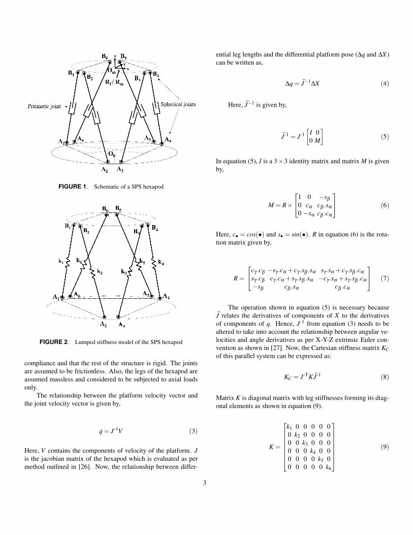
FIGURE 1. Schematic of a SPS hexapod

FIGURE 2. Lumped stiffness model of the SPS hexapod

compliance and that the rest of the structure is rigid. The jointsare assumed to be frictionless. Also, the legs of the hexapod areassumed massless and considered to be subjected to axial loadsonly.

The relationship between the platform velocity vector andthe joint velocity vector is given by,

q = J-1V (3)

Here, V contains the components of velocity of the platform. Jis the jacobian matrix of the hexapod which is evaluated as permethod outlined in [26]. Now, the relationship between differ-

ential leg lengths and the differential platform pose (∆q and ∆X)can be written as,

∆q = J−1∆X (4)

Here, J−1 is given by,

J-1 = J-1[

I 00 M

](5)

In equation (5), I is a 3×3 identity matrix and matrix M is givenby,

M = R×

1 0 −sβ

0 cα cβ .sα

0 −sα cβ .cα

(6)

Here, c• = cos(•) and s• = sin(•). R in equation (6) is the rota-tion matrix given by,

R =

cγ .cβ −sγ .cα + cγ .sβ .sα sγ .sα + cγ .sβ .cα

sγ .cβ cγ .cα + sγ .sβ .sα −cγ .sα + sγ .sβ .cα

−sβ cβ .sα cβ .cα

(7)

The operation shown in equation (5) is necessary becauseJ relates the derivatives of components of X to the derivativesof components of q. Hence, J-1 from equation (3) needs to bealtered to take into account the relationship between angular ve-locities and angle derivatives as per X-Y-Z extrinsic Euler con-vention as shown in [27]. Now, the Cartesian stiffness matrix KCof this parallel system can be expressed as:

KC = J-TKJ-1 (8)

Matrix K is diagonal matrix with leg stiffnesses forming its diag-onal elements as shown in equation (9).

K =

k1 0 0 0 0 00 k2 0 0 0 00 0 k3 0 0 00 0 0 k4 0 00 0 0 0 k5 00 0 0 0 0 k6

(9)

3

The matrix KC relates the 6×1 wrench vector ∆F applied at theplatform and the 6×1 platform displacement vector ∆X as,

∆F = KC∆X (10)

Equation (10) can be reorganized to get the following equation:

Ax = ∆X (11)

Here, x is a 6×1 vector that contains joint compliances 1/ki.

x = [1/k1,1/k2,1/k3,1/k4,1/k5,1/k6]T (12)

The 6×6 matrix A is a function of ∆F , J and J. The elements ofA are given by,

Aij = Jij(6

∑k=1

Jkj∆Fk) (13)

Here, i, j and k are the subscripts for the row and column ofrespective matrices. ∆Fk=1 to 6 refer to the components of wrenchapplied to the platform.

STIFFNESS IDENTIFICATION METHODMethod description

When we substitute the values of estimated lumped stiff-nesses (ki=1 to 6), wrench ∆F , hexapod jacobian J and J in equa-tion (11), we get the expected platform deflection ∆X . The sameequation can be used to identify lumped stiffness values when weknow everything in equation (11) except x. This implies load-ing the platform, measuring the platform deflection and solvingequation (11). If we increase the number of poses to be mea-sured, we get a 6n×1 x vector and a 6n×6 A matrix, where n isthe number of poses.

Fig. 3 shows the procedure for stiffness identification. Itconsists of the following steps:

1. Define experimental constraints that restrict the identifica-tion process. For example: workspace limits, loading limi-tations, etc.

2. Choose the number of poses and the number of measure-ments per pose. More number of measurements per posehelp to reduce the uncertainty of identified parameters at agiven pose due to measurement errors.

3. Identify the best set of poses (considering workspace con-straints) and corresponding external forces (consideringloading constraints) to identify the stiffness parameters. Thenext sub-section elaborates on the need and method forchoosing the optimal set of poses and forces.

4. Load the platform suitably at identified best poses and mea-sure the 6-DOF platform deflection.

5. Solve equation (11) to obtain the vector x. This can beaccomplished by minimizing the Euclidean norm of (Ax−∆X). The MATLAB function lsqminnorm can be used forthis purpose.

FIGURE 3. Procedure for stiffness identification

Algorithm to identify optimal set of poses and forcesThe idea behind having measurements at more number of

poses is the same as that for robot geometric calibration. Ingeometric calibration, measurements of large number of posesspread across the robot's workspace are used. These measure-ments are then used to get the best geometric parameter set thatminimizes the error between commanded and attained robot posethroughout the workspace. Large number of poses are neededfor this to reduce the influence of measurement errors. However,

4

practicality concerns demand reduction of these measurements.It has been shown that choosing the right set of measurementposes improves identification accuracy [28].

In our application, matrix A decides the quality of identifi-cation of parameters. This is because it relates the measurementsdone to the identified parameters. Since A is a function of X and∆F , the best parameters can be identified by judicious choiceof robot poses X and platform forces ∆F . Hence, the parame-ters need to be optimized for all reachable poses and allowableforces.

Parameter identification observability is a well-researchedtopic in robot calibration literature. However, stiffness parameteridentification observability is a relatively new area of research.Klimchik et al. [18] have presented a method to optimize the poseset for stiffness parameter identification to increase the accuracyof displacement prediction at just one particular pose. This is notsuitable for us since we seek to increase the accuracy of displace-ment prediction throughout the workspace of the hexapod.

Many observability indices can be found in the calibrationliterature: O1 [28], O2 [29], O3 [30], O4 [31] and O5 [32].The reliability and performance of these observability indiceshave been studied very well too [32–37]. There is no absoluteconsensus on the best observability index and also their perfor-mances have been noted to depend on the type of robot beingcalibrated [36]. Joubair et al. [34] have also shown that all theseobservability indices yield good result when the measurementnoise is low.

The observability indices also depend on the properties ofrobot models. Matrix scaling needs to be employed when param-eters for different variables with different units need to be iden-tified in calibration. Also, different scaling approaches producedifferent results. Only O1 is suitable for optimization of param-eter estimation with unscaled robot models. The mathematicalproof for this can be found in [32]. If this stiffness identificationtechnique is to be later included in a complete calibration tech-nique that also includes geometric parameters, the issue of matrixscaling can be more complex. Therefore, to avoid complicationsrelated to matrix scaling, it is advantageous to select O1 as theobservability index.

For stiffness parameter identification using equation (11),O1 is obtained by singular value decomposition of matrix A. Itcan be calculated as shown in [28],

O1 =(σ1σ2σ3....σp)

1/p√

N(14)

Here, p is the number of parameters to be identified which in ourcase is 6 and N is the number of poses. σ1 to p are the singularvalues of matrix A. The best set of poses and corresponding ex-ternal forces maximize the index O1. An optimization routinethen needs to be used to find the best set of poses and external

forces that maximize O1.

MEASUREMENT TECHNIQUEThis section elaborates on the measurement technique used

to measure the hexapod pose parameters in the experiments pre-sented in this paper. The measurement setup is as shown inFig. 4. The measurement system consists of a LK-METRIS co-ordinate measuring machine (CMM) with RENISHAW SP25Mscanning probe. Precision balls are glued to the hexapod for mea-surement of poses using the CMM. The procedure can be dividedinto two steps: (i) identifying the coordinate frame fixed to themobile platform, and (ii) measurement of poses using precisionballs. The interest here is to measure the 6-DOF parameters, X ,of the platform pose by measuring the positions of precision ballsin space.

The identification of reference frame fixed to the mobileplatform is done in the manner similar to the one describedin [38]. The reference holes on the hexapod are used for thispurpose. These reference holes are machined into the platformof the hexapod in the production phase. This is followed by mea-suring the positions of three precision balls with reference to themobile frame. These three balls’ positions can then be used asthree points in space to identify the mobile frame.

The measurement technique can be demonstrated using Fig.5. Let Pose 1 be the pose in which the precision balls are identi-fied in the mobile frame. Let PA1, PB1 and PC1 be the positions ofthe three precision balls associated with this pose and expressedin the mobile frame of reference. The pose vector X1 associatedwith this pose is [0,0,0,0,0,0]T . Let’s call this measurement M1.Now, when the platform moves to Pose 2, we carry out measure-ment M2 of the precision balls’ positions: PA2, PB2 and PC2. Theprecision balls' positions of measurement M2 are also expressedin mobile frame. A least square fitting algorithm is then used tosuperimpose the relative positions of the balls measured in M1on to the ball positions measured in M2. The mobile frame asso-ciated with Pose 2 can then be easily identified since the pose ofmobile frame relative to precision balls’ positions (PA1, PB1 andPC1) of Pose 1 is known. We now obtain Pose 2 (X2) with respectto Pose 1. Subsequent poses can then be measured with respectto Pose1. All this is done automatically using dedicated softwaretools developed by Symetrie. The 6-DOF deflection between theposes can be obtained by subtracting X1 from X2.

METHOD IMPLEMENTATION AND EXPERIMENTALVALIDATION

This section elaborates on how the stiffness identificationmethod was used to evaluate stiffness of a hexapod positionerfrom Symetrie. The product details cannot be disclosed due toconfidentiality. The test setup is as shown in Fig. 6.

5

FIGURE 4. Measurement setup

FIGURE 5. Pose measurement using precision balls

The experimental constraints included: (i) the allowableworkspace of the robot, and (ii) the loading constraint. Con-cerning the workspace constraints for identification, the platformcould not be rotated around its X and Y axes in addition to al-lowable workspace of the hexapod. This constraint was incor-porated to make sure that the mounted mass doesn't slide off theplatform. The loading constraint in this case was that the plat-form could only be loaded by placing mass on it. The load was,therefore, along the Z axis of the platform.

Now, the number of poses and number of measurements perpose had to be chosen. For any system of equations, the numberof equations should at least be equal to the number of unknowns.In this case, we have 6 unknowns and each pose measurementgives us six equations (6-DOF measurement). Hence, just onemeasurement is analytically enough to identify all parameters.

FIGURE 6. Experimental setup

For efficiency, it is also desirable to keep the number of posesfor identification less. Hence, compromising between efficiencyand accuracy, 3 poses and 3 measurements per pose were chosen.This choice would lead to a total of 9 measurements for identifi-cation. Given the nature of measurements in our case, this resultin 54 equations for 6 unknowns.

These choices and constraints lead to 13 design variables forthe optimization: twelve pose variables and one force variable.Concerning the load variable, ∆F3, further analysis revealed thatthe index O1 increased with increased magnitude of ∆F3 for anyrandom set of poses (Fig. 7). It was also observed that the hexa-pod has linear stiffness characteristics. Fig. 8 shows the resultsof an experiment that shows the hexapod's linear stiffness behav-ior. In this case, the hexapod platform was loaded only along itsZ-axis at pose [0,0,0,0,0,0]T . Due to these reasons, a choicewas made to use just one load vector of maximum possible mag-nitude to induce maximum platform deflection. This was 34.5kg in the given case. For displacement calculation, the refer-ence condition was a pre-load of 12.2 kg. This was necessaryto suppress the play in actuators. Hence, the effective load forwhich the platform deflection was measured was 22.3 kg alongthe Z-axis of the platform. It must be noted that in cases wherestiffness is considerably dependent on applied force, more load-ing conditions will have to be considered for this optimization.

Since the force variable was already chosen, the number ofdesign variables reduced to 12. MATLAB's f mincon functionwas then used to find the best set of 3 configurations that gavethe highest O1. These results are very sensitive to the startingpoint supplied to the optimization algorithm. To tackle this, par-

6

100 150 200 250 300

Vertical load on platform, ∆F3 (N)

50

100

150

200

Ob

serv

abil

ity

in

dex

, O

1

Pose set 1 Pose set 2 Pose set 3

FIGURE 7. Trend of O1 with respect to ∆F3

0 2 4 6 8 10 12

Platform deflection along Z-axis, ∆c (µm)

0

100

200

300

Fo

rce

alo

ng

Z-a

xis

, ∆

F3 (

N)

Trial 1 Trial 2 Trial 3

FIGURE 8. Plot showing linear stiffness behavior of hexapod understudy

allel computing was used along with large number of startingpoints to find the best solution. The best pose set for identifi-cation generated by this optimization is shown in table 1. Thehexapod was loaded in these poses and the platform deflectionswere measured. Equation (11) was then solved to get the stiffnessparameters which are tabulated in table 2.

TABLE 1. Best pose set for stiffness identification

a(mm) b(mm) c(mm) α(deg) β (deg) γ(deg)

Pose1 2.616 0.832 -0.666 0 0 15.756

Pose2 10.017 -3.434 -0.764 0 0 -11.007

Pose3 -7.784 -3.210 1.760 0 0 -11.266

The efficiency of this stiffness identification method wasthen validated using platform deflection measurements done atdifferent poses along the X and Y axes of the hexapod. Thedetailed description of poses is tabulated in table 3. The loadused was same as that for stiffness identification. Figures 9 and10 show the comparison between the predicted and measured 6-DOF deflections of the platform at different poses along the X

TABLE 2. Identified stiffness parameters

Stiffness parameter value (N/µm)

k1 k2 k3 k4 k5 k6

4.1981 3.7898 2.7503 4.3200 3.6716 3.7288

and Y axes of the hexapod, respectively. Table 4 shows the RMSvalues of error in prediction of the 6-DOF deflections.

TABLE 3. Pose set for experimental validation

Pose alongPose parameters

a(mm) b(mm) c(mm) α(deg) β (deg) γ(deg)

X-axis

-30

0 0 0 0 0

-15

0

15

30

Y-axis 0

-30

0 0 0 0

-15

0

15

30

TABLE 4. Error in deflection prediction (RMS values)

ε∆a 2.7 µm

ε∆b 3.1 µm

ε∆c 2.2 µm

ε∆α 6.4 µrad

ε∆β 8.3 µrad

ε∆γ 8.8 µrad

DISCUSSION AND FUTURE WORKValidation results show that the predicted and measured de-

flections of the platform are very close. As seen from table 4, theRMS values of prediction error is under 3.1 µm for translationaldeflections and 8.8 µrad for rotational deflections. This method

7

-25

-12.5

0

12.5

25∆a

-25

-12.5

0

12.5

25

Dis

pla

cem

ent

(µm

) ∆b

-30 -15 0 15 30

X-axis position (mm)

-25

-12.5

0

12.5

25∆c

-40

-20

0

20

40∆α

-40

-20

0

20

40R

ota

tion (

µra

d) ∆β

-30 -15 0 15 30

X-axis position (mm)

-40

-20

0

20

40∆γ

Prediction Measurement

FIGURE 9. Plot of predicted and measured 6-DOF deflection of hexa-pod under load at poses along X-axis

will also reduce the positioning inaccuracy due to compliance ofthe hexapod to the same level. This is due to the fact that themodel prediction accuracy is the only source of error in positioncompensation technique. This implies that the positioning errordue to compliance deflection will reduce, for example, along Z-axis translational coordinate of the hexapod from 13.5 µm (RMSvalue of measured ∆c) to 2.2 µm.

The small difference that exists between the prediction andthe measured values could be attributed to the following:

1. Uncertainty of measurement of the measurement system:All measurements have an uncertainty bound and this limitsboth stiffness parameter identification and the experimentalvalidation.

2. Geometric parameter error: The geometric parameters ofthe hexapod used for analysis was not calibrated. This isa source of error in parameter identification and experimen-tal validation. This is because of the use of an erroneousgeometric model to identify stiffness parameters from themeasurements and for predicting the displacements.

3. Incomplete stiffness model: The simple stiffness model usedcannot capture the complete compliance behavior of thehexapod. Consequently, there will be some residual errordue to unmodelled compliance.

For future works, the method presented in this paper will,firstly, be validated for other loading conditions such as loading

-25

-12.5

0

12.5

25∆a

-25

-12.5

0

12.5

25

Dis

pla

cem

ent

(µm

) ∆b

-30 -15 0 15 30

Y-axis position (mm)

-25

-12.5

0

12.5

25∆c

-40

-20

0

20

40∆α

-40

-20

0

20

40

Rota

tion (

µra

d) ∆β

-30 -15 0 15 30

Y-axis position (mm)

-40

-20

0

20

40∆γ

Prediction Measurement

FIGURE 10. Plot of predicted and measured 6-DOF deflection ofhexapod under load at poses along Y-axis

along X and Y axes of the platform. It will also be validatedfor other hexapod mounting conditions in which some or all legsare subjected to tensile loading. These studies are of interest tovalidate the efficacy of the presented method to improve accuracyof positioning in applications such as the one shown in [39]. Thismethod will then be extended to include geometric and thermalparameter models to further improve the positioning accuracy ofthe hexapod.

CONCLUSIONThis paper proposed a new efficient method to experimen-

tally evaluate the stiffness of hexapods. This can be used to ac-curately predict and correct its positioning error due to structuralcompliance. The method employed a simple lumped stiffness pa-rameter model which uses one spring per leg to mimic its com-pliance behavior. A stiffness identification procedure was out-lined to estimate the parameters of the proposed stiffness model.This method required small number of measurements. An opti-mization based on an observability index was used to generatethe best set of poses and external forces for stiffness parameteridentification. The efficiency of the presented method was evalu-ated using an experimental study performed on a hexapod basedmicro-positioner. This was done by comparing the predicted 6-DOF deflections of the platform with the measured deflections.Results showed that the chosen model with identified parame-

8

ters could predict and consequently allow to correct the platformdeflections of the tested hexapod very well. The RMS values ofprediction error in the validation experiments is under 3.1 µm fortranslational deflections and 8.8 µrad for rotational deflections.The method is shown to reduce the RMS of positioning error dueto compliance deflection, for example, along the Z-axis transla-tional coordinate of the hexapod from 13.5 µm to 2.2 µm.

ACKNOWLEDGMENTThis work has been supported by Agence nationale de la

recherche (ANR), France (Projet ANR-15-LCV3-0005). The au-thors hereby express their gratitude for the support. The authorswould like to thank Marielle Baud from Symetrie for the helpprovided in using CMM. The authors would also like to acknowl-edge the valuable inputs from Olivier Lapierre, Gilles Diolez,Pierre Noire and Tristan Caritey of Symetrie.

REFERENCES[1] Symetrie. Telescope mirror adjustment. http:

//www.symetrie.fr/en/applications-2/telescope-mirror-adjustment/. [Accessed:2018-03-08].

[2] Symetrie. Hexapods for synchrotrons. http://www.symetrie.fr/en/applications-2/synchrotrons/, [Accessed: 2018-03-08].

[3] Symetrie. High payload adjustment with high accuracy.goo.gl/4eJXqp. [Accessed: 2018-03-08].

[4] Merlet, J.-P., 2006. Parallel robots, Vol. 128. SpringerScience & Business Media.

[5] LIRMM-Symetrie. Posilab. http://www.lirmm.fr/posilab/.

[6] Dumas, C., Caro, S., Chrif, M., Garnier, S., and Furet, B.,2010. “A methodology for joint stiffness identification ofserial robots”. In 2010 IEEE/RSJ International Conferenceon Intelligent Robots and Systems, pp. 464–469.

[7] Lee, K. M., and Johnson, R., 1989. “Static characteris-tics of an in-parallel actuated manipulator for clamping andbracing applications”. In Proceedings, 1989 InternationalConference on Robotics and Automation, pp. 1408–1413vol.3.

[8] Klimchik, A., Chablat, D., and Pashkevich, A., 2014.“Stiffness modeling for perfect and non-perfect parallel ma-nipulators under internal and external loadings”. Mecha-nism and Machine Theory, 79, pp. 1 – 28.

[9] Corradini, C., Fauroux, J.-C., Krut, S., et al., 2003. “Eval-uation of a 4-degree of freedom parallel manipulator stiff-ness”. In Proceedings of the 11th World Congress in Mech-anisms and Machine Science, Tianjin (China).

[10] Majou, F., Gosselin, C., Wenger, P., and Chablat, D., 2007.

“Parametric stiffness analysis of the orthoglide”. Mecha-nism and Machine Theory, 42(3), pp. 296 – 311.

[11] Clinton, C. M., Zhang, G., and Wavering, A. J., 1997. Stiff-ness modeling of a stewart platform based milling machine.Tech. rep.

[12] Li, Y.-W., Wang, J.-S., and Wang, L.-P., 2002. “Stiffnessanalysis of a stewart platform-based parallel kinematic ma-chine”. In Proceedings 2002 IEEE International Confer-ence on Robotics and Automation (Cat. No.02CH37292),Vol. 4, pp. 3672–3677 vol.4.

[13] Deblaise, D., Hernot, X., and Maurine, P., 2006. “A sys-tematic analytical method for pkm stiffness matrix calcula-tion”. In Proceedings 2006 IEEE International Conferenceon Robotics and Automation, 2006. ICRA 2006., pp. 4213–4219.

[14] Chen, J., and Lan, F., 2008. “Instantaneous stiffness anal-ysis and simulation for hexapod machines”. SimulationModelling Practice and Theory, 16(4), pp. 419 – 428.

[15] Rebeck, E., and Zhang, G., 1999. “A method for evaluat-ing the stiffness of a hexapod machine tool support struc-ture”. International Journal of Flexible Automation andIntegrated Manufacturing, 7(3/4), pp. 149–166.

[16] Klimchik, A., Pashkevich, A., and Chablat, D., 2013.“CAD-based approach for identification of elasto-static pa-rameters of robotic manipulators”. Finite Elements in Anal-ysis and Design, 75, pp. 19 – 30.

[17] Carbone, G., and Ceccarelli, M., 2006. “A procedure for ex-perimental evaluation of cartesian stiffness matrix of multi-body robotic systems”. In 15th CISM-IFToMM Sympo-sium on Robot Design, Dynamics and Control, Romansy.

[18] Klimchik, A., Pashkevich, A., Wu, Y., Caro, S., and Furet,B., 2012. “Design of calibration experiments for identifi-cation of manipulator elastostatic parameters”. Journal ofMechanics Engineering and Automation, 2, pp. 531–542.

[19] Alici, G., and Shirinzadeh, B., 2005. “Enhanced stiffnessmodeling, identification and characterization for robot ma-nipulators”. IEEE Transactions on Robotics, 21(4), Aug,pp. 554–564.

[20] Klimchik, A., Furet, B., Caro, S., and Pashkevich, A., 2015.“Identification of the manipulator stiffness model parame-ters in industrial environment”. Mechanism and MachineTheory, 90, pp. 1 – 22.

[21] Dumas, C., Caro, S., Cherif, M., Garnier, S., and Furet,B., 2012. “Joint stiffness identification of industrial serialrobots”. Robotica, 30(4), p. 649659.

[22] Ceccarelli, M., and Carbone, G., 2005. “Numerical and ex-perimental analysis of the stiffness performances of parallelmanipulators”. In Second international colloquium collab-orative research centre, Vol. 562, pp. 21–35.

[23] Bonnemains, T., Chanal, H., Bouzgarrou, B.-C., and Ray,P., 2009. “Stiffness computation and identification of par-allel kinematic machine tools”. Journal of Manufacturing

9

Science and Engineering, 131(4), p. 041013.[24] Abele, E., Weigold, M., and Rothenbcher, S., 2007. “Mod-

eling and identification of an industrial robot for machiningapplications”. CIRP Annals, 56(1), pp. 387 – 390.

[25] Symetrie. Experts in metrology and positioning. http://www.symetrie.fr/en/company/. [Accessed:2018-03-08].

[26] Dombre, E., and Khalil, W., 2013. Robot manipulators:modeling, performance analysis and control. John Wiley& Sons.

[27] Ardakani, H. A., and Bridges, T., 2010. “Review of the 3-2-1 euler angles: a yaw-pitch-roll sequence”. Departmentof Mathematics, University of Surrey, Guildford GU2 7XHUK, Tech. Rep.

[28] Borm, J. H., and Menq, C. H., 1989. “Experimental studyof observability of parameter errors in robot calibration”.In Proceedings, 1989 International Conference on Roboticsand Automation, pp. 587–592 vol.1.

[29] Driels, M. R., and Pathre, U. S., 1990. “Significance ofobservation strategy on the design of robot calibration ex-periments”. Journal of Robotic Systems, 7(2), pp. 197–223.

[30] Nahvi, A., Hollerbach, J. M., and Hayward, V., 1994. “Cal-ibration of a parallel robot using multiple kinematic closedloops”. In Proceedings of the 1994 IEEE International Con-ference on Robotics and Automation, pp. 407–412 vol.1.

[31] Nahvi, A., and Hollerbach, J. M., 1996. “The noise ampli-fication index for optimal pose selection in robot calibra-tion”. In Proceedings of IEEE International Conference onRobotics and Automation, Vol. 1, pp. 647–654 vol.1.

[32] Sun, Y., and Hollerbach, J. M., 2008. “Observability indexselection for robot calibration”. In 2008 IEEE InternationalConference on Robotics and Automation, pp. 831–836.

[33] Horne, A., and Notash, L., 2009. “Comparison of poseselection criteria for kinematic calibration through simu-lation”. In Computational Kinematics-Proceedings of the5th International Workshop on Computational Kinematics,Springer, pp. 291–298.

[34] Joubair, A., and Bonev, I. A., 2013. “Comparison of the ef-ficiency of five observability indices for robot calibration”.Mechanism and Machine Theory, 70, pp. 254–265.

[35] Zhou, J., Kang, H.-J., and Ro, Y.-S., 2010. “Comparison ofthe observability indices for robot calibration consideringjoint stiffness parameters”. In Advanced Intelligent Com-puting Theories and Applications, Springer, pp. 372–380.

[36] Joubair, A., Tahan, A. S., and Bonev, I. A., 2016. “Per-formances of observability indices for industrial robot cal-ibration”. In 2016 IEEE/RSJ International Conference onIntelligent Robots and Systems (IROS), pp. 2477–2484.

[37] Joubair, A., Nubiola, A., and Bonev, I., 2013. “Calibra-tion efficiency analysis based on five observability indicesand two calibration models for a six-axis industrial robot”.SAE International Journal of Aerospace, 6(2013-01-2117),

pp. 161–168.[38] Zhang, G., Du, J., and To, S., 2016. “Calibration of a small

size hexapod machine tool using coordinate measuring ma-chine”. Proceedings of the Institution of Mechanical Engi-neers, Part E: Journal of Process Mechanical Engineering,230(3), pp. 183–197.

[39] Symetrie. Synchrotron Diffractometer. http://www.symetrie.fr/en/applications-2/synchrotron-diffractometer/. [Accessed:2018-03-08].

10

A New Efficient Stiffness Evaluation Method to Improve ...

Documents

Transcript of A New Efficient Stiffness Evaluation Method to Improve ...