COMMUNICATIONS IN NUMERICAL METHODS IN ENGINEERING, VOl. 10, 913-926 (1994)

A NEW ALGORITHM FOR FINDING A PSEUDOPERIPHERAL VERTEX OR THE ENDPOINTS OF

A PSEUDODIAMETER IN A GRAPH

GLAUCIO H. PAULINO Schooi of Civil and Environmental Engineering, Cornell University, ithaca, N. Y. 14853, U. S.A.

IVAN F. M. MENEZES Department of Civil Engineering, PUC-Rio

Rua MarquEs de Sio Vicente, 225, 22453, Rio de Janeiro, R.J. , Brazil

MARCEL0 GATTASS Department of Computer Science, PUC-Rio

Rua Marqu2s de Sio Vicente, 225, 22453, Rio de Janeiro, R. J., Brazil

SUBRATA MUKHERJEE Department of Theoretical and Applied Mechanics, Cornell University, Ithaca, N. Y . 14853, U.S.A.

SUMMARY Based on the concept of the Laplacian matrix of a graph, this paper presents the SGPD (spectral graph pseudoperipheral and pseudodiameter) algorithm for finding a pseudoperipheral vertex or the end-points of a pseudodiameter in a graph. This algorithm is compared with the ones by Grimes et al. (1990), George and Liu (1979), and Gibbs et al. (1976). Numerical results from a collection of benchmark test problems show the effectiveness of the proposed algorithm. Moreover, it is shown that this algorithm can be efficiently used in conjunction with heuristic algorithms for ordering sparse matrix equations. Such heuristic algorithms, of course, must be the ones which use the pseudoperipheral vertex or pseudodiameter concepts

1. INTRODUCTION

After the publication of the landmark paper by Cuthill and McKee (1969),' graph theory became a standard approach to reorder sparse matrix equations for reducing bandwidth, profile or wavefront. However, the success of most algorithms depends upon the choice of one or more starting vertices$. Peripheral vertices (i.e. vertices for which the eccentricity is equal to the diameter of the graph) have been shownzp3 to be good starting vertices for reordering algorithms. Since the location of peripheral vertices in graphs is computationally expensive, 4 9 5

most reordering algorithms use pseudoperipheral vertices (PVs) instead, i.e. vertices with the highest possible eccentricity. Examples of such algorithms are Reverse Cuthill-McKee (RCM), Gibbs-Poole-Stockmeyer (GPS), * Gibbs-King (GK), 6*7 Snay, Sloan, Medeiros

0 Recently, Paulino et al.25.26 have proposed a new class of spectral-based reordering algorithms, which d o not depend on the choice of a starting vertex. After having finished the manuscript, the authors became aware of similar independent work (on spectral envelope reduction) by Barnard et al.44 Their report was completed in October 1993 while our manuscript was submitted to the Int. j . numer. methods eng. in March 1993.

CCC 0748-8025/94/110913-14 0 1994 by John Wiley & Sons, Ltd.

Received August 1993 Revised April 1994

914 G. H. PAULINO, 1. F. M . MENEZES, M. GATTASS AND S. MUKHERJEE

et al., l o Fenves and Law, l 1 Hoit and Wilson, l 2 and Livesley and Sabin. l 3 Moreover, several papers have been published about algorithms for finding one or more starting vertices for renumbering the vertices of a graph, e.g. Cheng (1973),14 Gibbs et al. (1976),2 George and Liu (1979),15 Pachl (1984), l6 Smyth (1985)’ l 7 Kaveh (1990), l 8 and Grimes et al. l9

Other reordering algorithms that use the pseudoperipheral vertex concept are the refined quotient tree, the one-way dissection and the nested dissection in the sparse matrix package SPARSPAK.3 Note, however, that the use of the pseudoperipheral vertex concept is not restricted to reordering sparse matrix equations. This concept has applications in various fields such as geography,20 and mapping of finite element graphs onto processor meshes, (see Reference 21, page 1417).

This paper presents the SGPD (spectral graph pseudoperipheral and pseudodiameter) algorithm for finding a pseudoperipheral vertex or the end-points of a pseudodiameter in a graph. A pseudoperipheral vertex is an approximately peripheral vertex, i.e. an heuristic approximation to a peripheral vertex. Similarly, pseudodiametrical vertices are approximately diametrical vertices, i.e. heuristic approximations to the end-points of a diameter. Note that pseudodiametrical vertices are pseudoperipheral ones, but two pseudoperipheral vertices are not necessarily pseudodiametrical ones. This distinction is made here because some reordering algorithms use one pseudoperipheral vertex (e.g. RCM3), others use the end-points of a pseudodiameter (e.g. GPS,2 GK,6 Sloan,’ and Medeiros et al. lo), while still others use more than two pseudoperipheral vertices (e.g. Hoit and Wilson, l 2 and Snay8).

The remainder of this paper is organized as follows. Section 2 provides graph theoretical definitions, notations and a brief discussion about spectral techniques applied to graphs. Section 3 presents the SGPD algorithm. Section 4 outlines the main numerical aspects for the implementation of this algorithm. Section 5 presents some numerical examples using Everstine’s 22 collection of benchmark test problems. These examples include eccentricity verification and use of the SGPD in conjunction with some widely used graph reordering algorithms. The coupling of the SGPD with existing reordering algorithms yields new versions of these algorithms. The results obtained show the effectiveness of the proposed SGPD algorithm. Section 6 presents some considerations about computational efficiency. Finally, Section 7 concludes this work.

2. GRAPHS: DEFINITIONS, NOTATIONS AND SPECTRAL TECHNIQUES

The basic graph-theoretical background to this paper can be found in the excellent books by Harary *, 23 and CvetkoviC et al. 24 Further details about spectral techniques applied to graphs, and their association with the finite element method, can be found in References 25 and 26.

Let G = (V,E) be an undirected and connected graph. V = (u l , UZ, ..., v,) is a set of vertices with I V I =n; E = [el, el, ..., em) is a set of edges with I E I = rn, where 1 . 1 denotes the cardinality of the set. Edges are unordered pairs of distinct vertices of V. A labelling of G is a function f: V -+ D, where D is a collection of domain labels. Here, D = (1 ,2 , ..., I V I ] is used. The vertices may also be referred by their labels in the labelled graph.

Two vertices Ui and ui in G are adjacent if ( U i , ~ j ) E E. If W C V, the adjacent set of W, Adj(W), is

Adj(W) = ( U i E (V - W) I ( U i , Uj} E E, u ~ E W, i # j }

‘The more recent book by Buckley and H a r a r ~ , ~ ’ which is based on the classic book by Harary,” is also a good alternative reference in the field of graph theory.

A NEW ALGORITHM 915

If W = ( u ) , where u is a single vertex, the adjacent set of W is denoted by Adj(u) instead of Adj( (4).

A section-graph G(W, E(W)) of G(V, E) is a graph for which W C V and

E(W) = ( ( U i , u j ) EE 1 ~i E W, ~j E W]

A clique is a section graph whose vertices are pair-wise-adjacent. The degree of the set W is defined as deg(W) = 1 Adj(W) 1. Again, if W is a single vertex,

the degree of W is denoted by deg(u) instead of deg((u]). A path in a graph is an ordered set of vertices ( ~ 1 , UZ, ..., uP+l ) such that Uk and u k + 1 are

adjacent vertices for k = 1, 2, . . . , p . This path has length p , and it goes from u1 to up+l, which are the endpoints of the path.

The distance d(ui, uj) between two vertices in G is the length of the shortest path between them, i.e. d(ui, Uj) = min I path between V i and V j I.

The eccentricity e(u ) of a given vertex u in G is the largest distance between u and any other vertex of G , i.e.

e(u) = max( d(u, Vi) 1 Oi E V)

The diameter 6(G) is the largest eccentricity of any vertex in the graph, i.e.

6(G) = max(e(vi) I Ui E V]

A peripheral vertex u is the one for which its eccentricity is equal to the diameter of the

For a given vertex r c V, the rooted level ~ t r u c t u r e ~ ” ~ ~ (this is a crucial concept to many graph, i.e. e(u) = 6(G).

reordering algorithms) is the partitioning

L ( r ) = (Lo(r), L1(r), ..., Le(r)(r)l

such that: Lo@)= ( T I

L1 ( r ) = Adj(Lo(r)) Li(r)=Adj(Lj-I(r)-Li-z(r)), i = 2 , ..., e(r )

Note that uR‘L)o Lk(r) = V. The length of L ( r ) is e(r ) , and the width of L ( r ) is

W ( T ) = max ( 1 Li ( r ) 1, O < i < e(r ) )

The association of graphs with matrices is of special importance in this paper. The adjacency

The adjacency matrix A(G) = [aij] of a labelled graph G is defined as: (A), degree (D) and Laplacian (L) matrices are defined next.

1 if (ui, Uj)EE otherwise aij = [

The degree matrix D(G) = [dij] is the diagonal matrix of vertex degrees:

dij= [ p ( u i ) if i = j otherwise

The Laplacian matrix L(G) = [I,] is defined as:

L(G) = D(G) - A(G)

916 G. H. PAULINO, I . F. M . MENEZES, M . GATTASS AND S. MUKHERJEE

or, in component form, L(G) is given by

if(u;, v,) E E l i j = deg(u;) if i = j io‘ otherwise

According to Anderson and Morley,29 the name ‘Laplacian matrix’ comes from a discrete analogy with the Laplacian operator in numerical analysis (for further explanation, see Paulino et ~ 1 . ~ ’ ) . The Laplacian matrix is symmetric, singular (each row or column sum up to zero), and positive-semi-definite. 29,30 It is employed here for the study of spectral properties of a graph.

Let the eigenvalues of L(G) be arranged in ascending order of their values:

O = X 1 < X z < - . * < A n < IVI

For the first eigenpair, ( X I , y1) = (0, l), where 1 is a unit vector, and the eigenvector y1 has been normalized. The special properties of the second eigenpair ( X 2 , y2) of L(G) have been studied by Fiedler. 3 0 ~ 3 1 He designates A2 as the algebraic connectivity of the graph G, which is related to the usual vertex and edge connectivities of G. If the graph has a simple pattern, analytical solutions are available for X 2 . 2 9 3 3 0 The components of y2 can be assigned to the vertices of G and can be considered as weights for them. Fiedler designates this weighting process as the characteristic valuation of G. It is determined uniquely up to a non-zero factor if X2 is a simple eigenvalue of L(G) (i.e. with multiplicity = 1).

3. THE SPECTRAL GRAPH PESUDOPERIPHERAL AND PSEUDODIAMETER (SGPD) ALGORITHM

The automatic algorithm SGPD is presented in Table I. A similar algorithm for finding a pseudoperipheral vertex in a graph has been proposed by

Grimes et af . l 9 and Kaveh. l 8 However, they have used a modified adjacency matrix B instead of the Laplacian matrix L. The matrix B is defined as

(2)

where I is the identity matrix (compare equation (2) with equation (1))t. Note that the eigenvalues of B are the ones for A shifted by unity, and the normalized eigenvectors of A and B are the same. Grimes et af . l9 and KavehI8 have used the vertex corresponding to the smallest component in the dominant eigenvector of B(G) as a pseudoperipheral vertex. Straffin2’ has used the vertex corresponding to the largest component in the dominant eigenvector of B (G)

B(G) = I(G) + A(G)

Table I. Spectral graph pseudoperipheral and pseudodiameter (SGPD) algorithm

1 . Find the eigenvector y2 of the Laplacian matrix L(G). 2. The vertex corresponding to the smallest (or largest) component in y2 is a pseudoperipheral vertex.

The vertices corresponding to the smallest and largest components in y2 are the endpoints of a pseudodiameter.

?Booth and Lipton’ call the above matrix B the ‘augmented adjacency matrix’. In their work, they also justify the use of this matrix instead of the standard adjacency matrix A.

A NEW ALGORITHM 917

@- Figure 1 . Grimes et a/. l9 counterexample

to determine the most accessible vertex in a graph network for an interesting application in geography. Note that the concept of most accessible vertex is opposed to the concept of pseudoperipheral vertex.

Figure 1 shows the counterexample presented by Grimes el al. I' Their algorithm fails for this problem, while the SGPD furnishes the optimal solution. The vertices in the two cliques at the left- (UI, u2, u3) and right- (US, US, u10) hand sides of Figure 1 are peripheral. The dominant eigenvector y I v I ( 1 V I = 10) of B corresponding to the largest eigenvalue (Xlvl=4-1284) is

yTVi(B) = L0.1073, 0.1073, 0.1073, 0.1211, 0.0569, 0.0569, 0.1211, 0.1073, 0.1073, 0.1073J (3)

The smallest components of ylvl(B) correspond to the interior vertices u5 and u6, which are inconsistent with the objective of the algorithm of finding peripheral or nearly peripheral vertices. With respect to Figure 1 and the SGPD algorithm of Table I, the eigenvector y2 of L corresponding to the algebraic connectivity of the graph (i.e. the second smallest eigenvalue: X2 = 0.1442) is

yT(L) = Ll.OOOO, 1.0000, 1.0000, 0.8558, 0.2997, -0.2997, -0.8558, -I.OOO, -l .OOOO, -1.OOOOJ (4)

The smallest components of y2(L) correspond to the clique (US, u g , U I O ) at the right-hand side of Figure 1 , and the largest components of y2(L) correspond to the clique (UI, UZ, u3) at the left-hand side of Figure 1 . In this case, the SGPD captures the essential structure of the graph and provides a peripheral vertex (e.g. US), or the end-points of a diameter (e.g. US and u l ) .

For this specific example, it is interesting to relate Figure 1 and the eigenvectors in expressions (3) and (4). Note that the components of y lv~(B) (equation 3) are symmetric, while the components of y2(L) (equation (4)) are skewsymmetric. For the SGPD algorithm (Table I), this last property is essential for obtaining the endpoints of a pseudodiameter (in this case, the actual diameter) of the graph in Figure 1 (it is worth mentioning that this last property is also related to Theorem 2.1 of Reference 32, p. 432).

3. SOME NUMERICAL ASPECTS

The numerical procedure which implements the SGPD algorithm (see Table I) should be able to handle large and generic graphs. Therefore, the main task in the SGPD is the solution of a large eigenproblem. The goal is the determination of the second eigenpair (XZ, y2) of the Laplacian matrix L. Here, the eigensolution is accomplished by a special version of the Subspace Iteration method, as reported by Paulino et aI.26 However, any other equivalent method can be used for the eigensolution, e.g. the Lanczos methods. 33p34 A brief description of the Subspace Iteration method, as implemented in this work, is presented next.

918 G. H. PAULINO, I . F. M. MENEZES, M. GATTASS AND S. MUKHERJEE

Since the interest here is in the eigenvector associated to the second eigenvalue of the Laplacian matrix L, the dimension suggested for the reduced subspace in the case of a connected graph is q = 4. 26 However, if necessary, the dimension of the reduced space (q) can be changed. So, the reduced eigenproblem is solved by QR iterations applied to matrices of order q. To solve the problem of singularity in the computation of the eigenvector corresponding to the null eigenvalue, the Laplacian matrix has been shifted according to

L + L + a I

where a is a shifting constant. Here, a = 1 has been adopted, such that all the eigenvalues become positive ( X j 2 1 -0; 1 < j < I V I ). This procedure does not change the normalized eigenvectors of the Laplacian matrix.

The convergence criterion is defined in terms of the relative error between successive eigenvalue approximations:

where the subscript denotes the j th eigenvalue, the superscripts denote the iteration numbers, and TOL is a specified tolerance for both the Subspace iterations and the QR iterations in the reduced space. 25p26 Each eigenvector approximation is normalized with respect to the absolute value of its largest component. Here, the number of iterations for both the Subspace and the QR methods are unlimited in a numerical sense, i.e. the maximum number of iterations has been chosen to be a very large number.

5 . EXAMPLES

Two types of numerical examples are presented next. Firstly, the eccentricity of the vertices obtained by the SGPD algorithm (Table I) is compared with the results of other heuristic algorithms and the actual diameter of the graph. Secondly, the vertices obtained by the SGPD are used as starting vertices of some widely used algorithms for bandwidth, profile and wavefront reduction. For the solution of the eigenproblem in the SGPD algorithm, TOL =

All the examples that follow come from the collection of benchmark test problems provided by Everstine.22 The matrices range in order from 59 to 2680. Larger test problems, e.g. with matrices of order around 40,000 and 1,000,000 entries, can be found in the Harwell-Boeing sparse matrix collection. 35 In fact, Everstine’s test problems are also included in this collection.

Everstine’s 22 collection of examples contains a set of 30 diversified problems representing finite element meshes, which have been widely used to test reordering algorithms. 9*22,26,36 A description of the test problems, and plots of the corresponding meshes, can be found in Everstine’s paper. 22 Here, the primary concern is connected graphs. Therefore, the SGPD algorithm will be tested using the test problems for which the associated nodal graph G is connected, i.e. 24 examples of Everstine’s collection. The other six examples are associated to non-connected graphs (A2 = 0) and are not treated here. Techniques for treating non-connected graphs, in the context of spectral methods, have been presented by Paulino et

(Equation ( 5 ) ) has been adopted.

5. I . Eccentricity verification

George and Liu” (here designated G&L), Gibbs et Table I1 lists some initial data about Everstine’s 22 test problems and the results obtained by

(here designated GPSD in order to

Tab

le 1

1. E

ccen

trici

ty c

ompa

riso

n am

ong

G&

L, G

PSD

and

SG

PD a

lgor

ithm

s

1 2

3 4

5 6

7 8

9 10

11

12

13

14

Gra

ph

G&

L G

PSD

SG

PD

IEI

A2

6(G

) PV

e(

PV)

PV1

59

66

72

87

162

193

209

22 1

245

307

310

361

419

503

592

758

869

878

918

992

1005

10

07

1242

26

80

104

127 75

227

510

1650

76

7 70

4 60

8 11

08

1069

12

96

1572

27

62

2256

26

18

3208

32

85

3233

78

76

3808

37

84

4592

11

173

0.0666

0.01

15

0-02

15

0 * 0

969

0.05

77

0.81

47

0.12

1 1

0.02

56

0-03

54

0.16

05

0.01

64

0.03

58

0.03

62

0.10

01

0.02

01

0.00

25

0.00

78

0.01

47

0.00

85

0.05

90

0.03

04

0.01

04

0-01

59

0.00

46

13

6 32

21

21

72

13

31

22

13

5 7

47

12

32

27

154

17

146

14

5 39

30

4 30

31

3 22

31

2 23

12

37

26

3 10

5 23

3 57

58

1 40

84

1 42

83

4 30

48

1 34

71

3 47

99

4 31

25

9 75

24

3

13

43

32

1 21

1

13

31

22

158

7 1

12

118

27

154

17

146

13

286

39

1 30

1

22

390

23

12

37

185

105

756

57

1 40

1

42

5 30

1

34

713

47

26

31

1 75

24

3

13

5 32

21

21

72

13

59

22

13

5 7

186

12

15

27

131

17

2 13

15

39

30

4 30

31

3 22

30

7 23

39

3 37

26

3 10

5 23

3 57

69

1 40

84

9 42

70

2 30

48

7 34

61

9 47

99

1 31

25

9 75

24

70

13

32

21

13

22 7 12

27

17

13

39

30

22

23

37

105 57

40

42

30

34

47

31

75

1 1 57

31

122

193 14

155 2

126 1 1

386

393

185 16 1

84 1

704

48 1

525

994

259

2489

13

6 32

21

19

1

13

59

21

158

7 16

2 12

15

27

19

8 17

14

6 13

79

39

31

0 30

31

3 22

31

1 23

12

37

26

3 10

5 75

8 57

58

1 40

1

41

5 30

16

33

69

7 47

1

31

8 73

24

2

13

32

21

13

22

9

12

E 7

5

27

17

39

4

l3

g 30

*

22

23

37

105 57

40

42

30

33

47

31

74

920 G. H. PAULINO, I. F. M. MENEZES, M. GATTASS AND S. MUKHERJEE

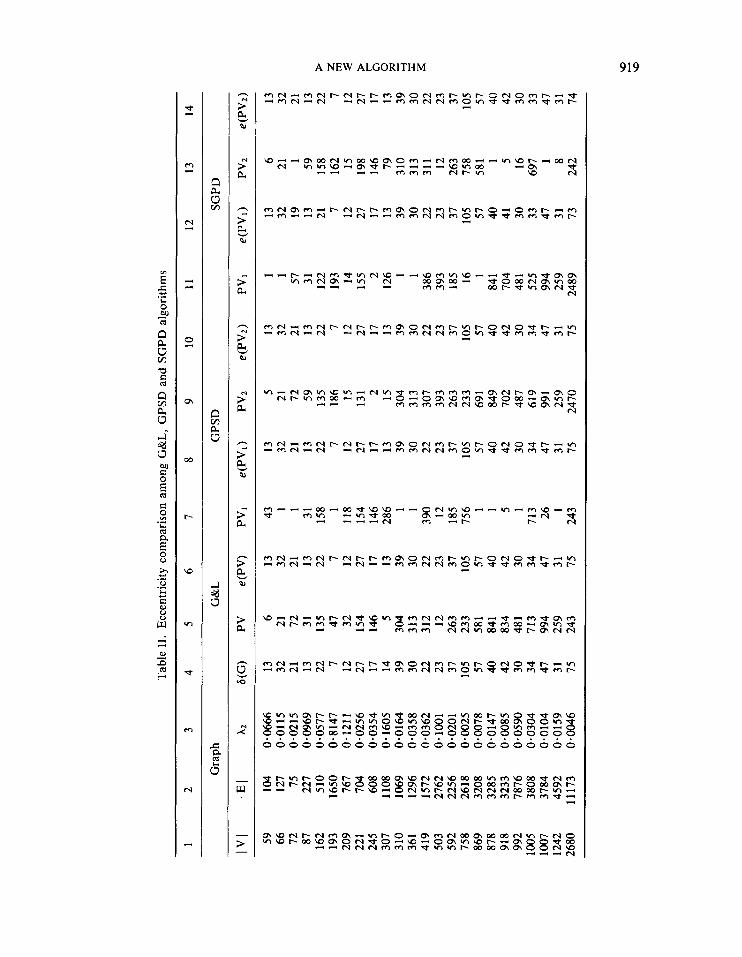
differentiate it from the GPS reordering algorithm), and the proposed SGPD (Table I) algorithm. The initial data are I V 1, I E I, algebraic connectivities (X2), and the diameters of the associated graphs (6(G)). The results are the pseudoperipheral vertices (PVI ) and respective eccentricities obtained by G&L, and the pseudodiametrical vertices (PV1 and PV2) and respective eccentricities obtained by GPSD and SGPD.

From Table 11, one observes that in some cases the pseudodiametrical vertices obtained by the GPSD and SGPD algorithms coincide, e.g. I V I = 66, 87, 245, 361, 503 and 592. In many cases, there are common pseudoperipheral vertices for G&L, GPSD and/or SGPD algorithms, e.g. I V I = 59, 66, 72, 87, 162, 209, etc.

Moreover, Table I1 also shows that the eccentricities obtained by the SGPD are comparable to those of G&L and GPSD algorithms. In most cases, the eccentricities obtained by the G&L, GPSD and SGPD algorithms are equal to the diameter of the graph. In 18 occasions, the SGPD gives e(PV1) = 6(G); for the other six occasions, e(PV1) is very close to 6(G) - the maximum difference between these quantities is 2. In 21 occasions, the SGPD gives e(PV2) = 6(G); for the other three occasions, the difference between 6(G) and e(PV2) is 1. The pseudodiametrical vertices of the GPSD algorithm satisfy the condition e(PV1) = e(PV2). In the case of the SGPD, this condition is satisfied in 20 occasions; for the other four occasions, the difference between e(PV2) and e(PVl) is 2 in one occasion, and 1 in the other three occasions.

5.2 Application to bandwidth, projile and wavefront reduction algorithms

The definitions used here for matrix bandwidth B, profile P and root mean square (r.m.s.) wavefront Ware the same as those provided by Everstine22 or Paulino et al. 26 In this section, the vertices obtained by the SGPD algorithm are used as trial starting vertices for the RCM (Table III), GPS (Table IV) and GK (Table V) algorithms.

Table 111. Reverse Cuthill-McKee (RCM) algorithm

1. Find a pseudoperipheral vertex. 2. Renumber this vertex as 1. 3. For i = 1, ..., I V I find all the unnumbered vertices in Adj(oi) and

label them in increasing order of degree. 4. For i = 1, ..., 1 V j revert the numbering by setting ( i ) to (n - i + 1).

~ _ _ _ _ _ _ _ _ ~~~

Table IV. Gibbs-Poole-Stockmeyer (GPS) a l g ~ r i t h r n ~ ~ ~ ’

1. Find endpoints of a pseudodiameter. 2. Minimize level width. 3. Number the graph in a manner similar to the RCM algorithm.

Table V. Gibbs-King (GK) algorithm2v6

1. Find endpoints of a pseudodiameter. 2. Minimize level width. 3. Number the graph level by level in a manner analogous to King’s criteria.’

A NEW ALGORITHM 92 1

The original version of the RCM algorithm uses the G&L” pseudoperipheral vertex. The original version of the GPS and GK algorithms uses the GPSD’ pseudodiametrical vertices. In the examples that follow, the original version of Step 1 of the RCM, GPS and GK algorithms (Tables 111, IV and V, respectively) is replaced by the SGPD algorithm. Note that coupling of the SGPD with the RCM, GPS and GK algorithms yields new versions of these reordering algorithms, which are designated here as RCM(SGPD), GPS(SGPD) and GK(SGPD), respectively.

Table VI lists I V 1 , the initial values of B, P and W, the results for B, P and W using the original RCM, and the results for B, P and Wusing the RCM with the SGPD algorithm. These last results are obtained as the ones which give the smallest profiles when PV1 and PV2 (see 1 Ith and 13th columns of Table 11) are used as starting vertices. The strategy of using two trial starting vertices is efficient because the simple and easily accessed data structure of the RCM (see Table 111) makes it an extremely fast reordering algorithm. 3,19,26 For the RCM algorithm, Table IV shows that, on the average, the SGPD is more effective than the G&L algorithm.

Table VII lists I V I and the normalized values of B, P and W for the RCM, GPS and GK algorithms. The relative values of B, P and W are the ratio of the results obtained with the reordering algorithm using the SGPD starting vertices and the ones obtained with the original reordering algorithm. The relative values of B, P and W for the RCM algorithm can be

Table VI. Bandwidth, profile and wavefront reduction using the RCM and the RCM(SGPD) algorithms

1 2 3 4 5 6 7 8 9 10

Initial RCM RCM(SGPD) Problem

I V I B P w B P w B P w

59 66 72 87

162 193 209 22 1 245 307 310 361 419 503 592 758 869

26 45 13 64

157 63

185 188 116 64 29 51

357 453 260 20 1 587

464 640 244

2336 2806 7953 9712

10131 4179 8132 3006 5445

40145 36417 29397 23871 20397

8.219 11.008 3.460

29.378 18.955 43-841 50.322 50.393 18.481 27 * 360 9.852

15.379 107-072 78.603 55.179 37.946 25.019

9 4 8

19 17 50 34 20 58 45 16 16 34 60 43 29 44

315 223 356 710

1641 5153 3804 2367 5587 865 1 3141 5075 8609 4906 1452 8718 9259

878 520 26933 31.921 47 22385 918 840 109273 131.142 58 23096 992 514 263298 301-994 66 38128

1005 852 122075 137.660 105 43106 1007 987 26793 26.925 39 24703 1242 937 111430 105.201 93 50241 2680 2500 590543 234.418 70 105798

5 * 469 3.435 5.231 8-669

10.532 28-097 19.185 11.349 25-901 29.668 10.363 14.277 21 a21 1 31.759 20.657 13.018 24.169 26.610 26.743 40.125 48.902 25.427 42-425 40.632

9 4 9

22 18 57 34 16 46 42 15 16 39 60 43 29 42 38 62 64

103 39 93 70

315 223 382 699

1612 4974 3812 2164 4472 81 15 3035 5075 8474

14906 11452 8581

16949 22007 22984 37288 42398 24703 5024 1

10626 1

5.469 3.435 5.627 8.561

10.378 26,881 19.216 10.198 19-815 27.339 9.958

14.277 21 a058 31.759 20.657 12.818 21.650 25.923 26.998 39.088 47.066 25.427 42.425 40.739

922 G. H. PAULINO, 1. F. M. MENEZES, M. GATTASS AND S. MUKHERJEE

Table VII. Relative bandwidth, profile and wavefront reduction using the RCM, GPS and GK algorithms

1 2 3 4 5 6 7 8 9 10

RCM(SGPD) GPS(SGPD) GK(SGPD)

RCM GPS GK Problem

IVI B P w B P w B P w 59 1.000 66 1.OOO 72 1.125 87 1.158

162 1 a059 193 1.140 209 1.OoO 22 1 0.800 245 0.793 307 0.933 3 10 0.937 361 1 *000 419 1.147 503 1.OOO 592 l*OOO 758 l-OOO 869 0.954 878 0.808 918 1.069 992 0.970

1005 0-981 1007 1.000 1242 1.000 2680 1.000

1 ,OoO 1.OoO 1-073 0 * 984 0.982 0.965 1 a002 0.914 0.800 0.938 0.966 1 a 0 0 0 0.984 1.OOO 1.OoO 0.984 0.880 0.983 0-995 0.978 0-984 1.OoO 1.OOO 1-004

1.OOO 1 a 0 0 0 1-076 0.987 0.985 0.957 1.002 0 899 0.765 0.921 0.961 1 *000 0.993 1.OOO 1.OOO 0.985 0.896 0.974 1.009 0.974 0.962 1.000 1 a 0 0 0 1.003

0.889 1.OOO 1.286 0.850 1.071 1-302 0.767 0.895 1.OOO 1.023 0.933 1.000 1.206 1 a 0 0 0 1.000 1.000 1 s o 0 0 1 *ooo 1-180 1.OoO 0.963 0.914 0.970 1.014

0.909 1-OoO 1.127 0.952 0.993 1 a023 0.772 0-964 1 *om 0.966 0-991 1 a 0 0 0 0.981 1.OOO 0.997 0 999 1-OOO 0.994 1.027 1-000 1.006 0 996 0-963 1.016

0.894 1.OoO 1.151 0.942 1 a002 1 *027 0-752 0.959 1.OoO 0 * 947 0.990 1 .000 0 * 992 1.OoO 0.993 0.999 1.000 0.994 1.047 1.OoO 1 a001 0.993 0.961 1.017

0.833 1.OOO 1.000 0.810 1.OOO 1.196 0.939 0.857 1.000 1.125 0-727 1.OoO 1.143 0.986 1.OOO 1 *om 1.OOO 1.OOO 1 - 185 1.OOO 0.824 0.800 0.815 0.989

0.917 1.OoO 1.217 0.829 1.004 1.060 0.767 0.943 1*OOO 0.946 0.993 1.OOO 1.002 0.971 1.OOO 1,OoO 1.OoO 1.OoO 1.075 1.OOO 0.971 1 *003 0.882 1.048

0.901 1.000 1-247 0.809 1 *012 1 -065 0.757 0.938 1.000 0-935 0.993 1.000 1.012 0 * 966 1.000 1.000 1.000 1-000 1 * 106 1.000 0.946 1 a002 0.875 1.053

Average 0.995 0.976 0.973 1-011 0.987 0.986 0.968 0-985 0.984 WlL 816 1413 1314 8/7 1315 1216 1014 917 917

obtained directly from Table VI (ratios of 8th and 5th, 9th and 6th, and 10th and 7th columns, respectively).

Note that, for all the columns in Table VII, the number of occasions in which the reordering algorithms with the SGPD are better (ratio < 1-0) for B, P and l@ reduction, is larger than the number of occasions in which the original reordering algorithms are better (ratio > 1.0). These global quantitative results are shown in the last row of Table VII, where W (wins) means the number of occasions that the reordering algorithm with the SGPD (Step 1 in Tables 111-V) wins against the original algorithms, and t (losses) means the number of occasions that the reordering algorithms with the SGPD loses against the original algorithms.Obviously, this comparison excludes ties (ratio = 1 -0).

From Table VII, the following conclusions can be obtained in a general sense. For the RCM reordering, the SGPD is more effective than the G&L algorithm; for the GPS reordering, the SGPD is slightly better than the GPSD algorithm; for the GK reordering, the SGPD is also slightly better than the GPSD algorithm.

A NEW ALGORITHM 923

6 . SGPD ALGORITHM RUNNING TIME PERFORMANCE

The numerical procedure which implements the SGPD algorithm (see Table I) has been presented in Section 4 and applied to numerical examples in Section 5 . We have observed that the proposed eigensolution scheme makes the SGPD algorithm very time-consuming when compared to G&L3*” and GPSD’ algorithms. The following three strategies may significantly reduce the SGPD running time: (1) tuning of convergence parameters; (2) change of the eigensolver; (3) vectorization/parallelization of the SGPD algorithm.

6.1. Tuning of convergence parameters

The goal of the SGPD algorithm (Table I) is to determine the locations of the smallest and largest eigenvector components in yz(L) and not their actual values. Therefore, an accurate numerical solution of the eigenproblem may not be necessary. In many cases, a reasonable approximation to yz(L) may suffice for the purposes of the SGPD algorithm. Hence, the convergence criterion (equation ( 5 ) ) may be relaxed in favour of computational efficiency. This means that, in equation (9, the tolerance can be bigger than the default value TOL = adopted previously.

To make the point stated above, a typical example is presented next. Consider the problem with I V I = 503 in Table 11. The convergence verification for this problem is illustrated by Table VIII, which shows some preliminary information and the convergence results. The preliminary information includes 1 V 1, 1 E 1, 6(G) and the initial values for B, P and W. The convergence results are: the adopted tolerance (TOL); the CPU time (seconds); XZ; PVI, e(PVI), and the RCM results for B, P and W using PVI as the starting vertex; and similarly, PVZ, e(PV2), and the RCM results for B, P and @using PVZ as the starting vertex. The goal here is to assess the quality of the results for eccentricity and for B, P and Was the tolerance is increased. Note that, in this case, the pseudodiametrical vertices obtained with TOL =

Table VIII. Computational efficiency (HP apollo 9000-720)

Preliminary information

IVI 1El W) P w B

503 2762 23 36417 78-603 453

RCM(SGPD)

TOL Time XZ #Iter. PVI e(PV1) B P W PV2 e(PV2) B P w 6)

~ ~

96.23 0.1001 108 393 23 67 16667 36.114 12 23 60 14906 31.759 15.09 0.1082 16 393 23 67 16667 36-114 12 23 60 14906 31.759

lo-’ 9 .04 0.1480 9 393 23 67 16667 36.114 12 23 60 14906 31.759 l o - ’ 5.62 0.2023 5 274 16 65 18370 37.912 81 22 68 17657 38.415

924 G. H. PAULINO, 1. F. M. MENEZES, M. GATTASS AND S. MUKHERJEE

or TOL = results. Moreover, from TOL = order of magnitude.

do not change. However, even if they change, they may still be acceptable the SGPD running time is reduced by an to TOL =

6.2. Change of the eigensolver

The dominant computation in the SGPD algorithm (Table I) is the determination of the eigenvector associated to the second eigenvalue of the Laplacian matrix. In this paper, the eigenproblem has been solved by the subspace iteration method as presented by Paulino et al. ” It is worth investigating alternative eigensolvers (together with specific characteristics for improved computational efficiency) to be used by the SGPD algorithm. Promising candidates are Lanczos-type methods. 33,34,38-43

A comparison between Lanczos and subspace iteration methods has been presented by Nour-Omid et al.33 and Sehmi (Reference 34, p. 68). Simon3* and Hsieh et have used the Lanczos method to determine y2 (L) in recursive domain partitioning algorithms (bisection- type) for parallel finite element analysis. Recently, Barnard and Simon4’ have reported an improved multilevel implementation of this algorithm that is an order of magnitude faster than the one reported in Reference 38. Hendrickson and have used additional eigenvectors of the Laplacian matrix, besides y2(L), to obtain higher-order partitions (quadrisection-, octasection-type algorithms). They have also developed an efficient multilevel algorithm for partitioning graphs.43 However, investigation of these algorithms (Lanczos- type),33334*38-43 in the context of the present SGPD algorithm (see Table I), is a subject for future research.

6.3. Vectorizationl parallelization

The numerically intensive part of the SGPD algorithm (Table I) involves standard vector operations using floating-point arithmetic (this is in contrast to other algorithms based on the level structure concept and using integer arithmetic). Therefore, this algorithm is well suited for computers with vector processors. Moreover, the algebraic nature of the algorithm favours its implementation in a parallel computing environment. For example, at Cornell Theory Center, we have available a computing environment that includes vector-scalar super- computing resources and parallel systems such as the IBM ES/9000-900. The investigation of the SGPD as well as other numerical algorithms in advanced computing environments is also a subject for future research.

7. CONCLUSIONS

A new algorithm (SGPD) has been proposed for finding a pseudoperipheral vertex or the end- points of a pseudodiameter in a graph. Based on comparative studies, this algorithm is, in general, more effective than the ones presented by Grimes et al., l9 George and Liu (G&L), l5 and Gibbs et al. (GPSD).’

ACKNOWLEDGEMENTS

The first author acknowledges the financial support provided by the Brazilian agency CNPq. Ivan F. M. Menezes acknowledges the financial support provided by CAPES, which is another

A NEW ALGORITHM 925

Brazilian agency for research and development. Most of the computations in the present work have been performed in CADIF (Computer Aided Design Instructional Facility), at Cornell University. The authors are especially grateful to Catherine Mink, CADIF Director, for giving credit to the ideas presented to her and for providing the resources necessary to carry out this research. The excellent computing system support by John M. Wolf, from CADIF, is also acknowledged. Dr Gordon C. Everstine, from David W. Taylor Model Basin (Department of the Navy), has given the authors a computer tape with his collection of benchmark problems for testing nodal reordering algorithms. The first author thanks Dr Shang-Hsien Hsieh for useful discussions about computational graph theory. The authors thank Mr Khalid Mosalam for carefully reading the manuscript, for his constructive criticism and valuable suggestions to this work.

REFERENCES 1 . E. Cuthill and J. McKee, ‘Reducing the bandwidth of sparse symmetric matrices’, ACM Proceedings

of 24th National Conference, ACM Publication P-69, 1969, pp. 157-172. 2. N. E. Gibbs, W. G. Poole, Jr. and P. K. Stockmeyer, ‘An algorithm for reducing the bandwidth

and profile of a sparse matrix’, SIAM J. Numer. Anal. 13, (2), 236-250 (1976). 3. A. George and J. W.-H. Liu, Computer Solution of Large Sparse Positive Dejnite Systems,

Prentice-Hall, New Jersey, U.S.A., 1981. 4. W. F. Smyth and W. M. L. Benzi, ‘An algorithm for finding the diameter of a graph’, in J. L.

Rosenfeld (Ed.), Proceedings of IFIP Congress 74, North-Holland Publ. Co., 1974, pp. 500-503. 5. K. S. Booth and R. J. Lipton, ‘Computing extremal and approximate distances in graphs having unit

cost edges’, Acta I f . , 15, 319-328 (1981). 6. N. E. Gibbs, ‘Algorithm 509 - A hybrid profile reduction algorithm,’ ACM Trans. Math. Softw.

7. I. P. King, ‘An automatic reordering scheme for simultaneous equations derived from network systems’, Int. j numer. methods eng., 2, 523-533 (1970).

8. R. A. Snay, ‘Reducing the profile of sparse symmetric matrices’, Bull. Ggod., 50, (4), 341-352 (1976).

9. S. W. Sloan, ‘A FORTRAN program for profile and wavefront reduction’, Inter. j . numer. methods eng., 28, 2651-2679 (1989).

10. S. R. P. Medeiros, P. M. Pimenta and P. Goldenberg, ‘An algorithm for profile and wavefront reduction of sparse matrices with a symmetric structure’, Eng. Comput., 10, (3), 257-266 (1993).

1 1 . S. J. Fenves and K. H. Law, ‘A two-step approach to finite element ordering’, Int. j . numer. methods eng., 19, 891-911 (1983).

12. M. Hoit and E. L. Wilson, ‘An equation numbering algorithm based on a minimum front criteria’, Comput. Struct., 16, (1-4), 225-239 (1983).

13. R. K. Livesley and M. A. Sabin, ‘Algorithms for numbering the nodes of finite-element meshes’, Comput. Syst. Eng., 2, (l), 103-114 (1991).

14. K. Y. Cheng, ‘Note on minimizing the bandwidth of sparse, symmetric matrices’, Computing, 11,

15. A. George and J. W.-H. Liu, ‘An implementation of a pseudoperipheral node finder’, ACM Trans.

16. J. K. Pachl, ‘Finding pseudoperipheral nodes in graphs’, J. Comp. Syst. Sci., 29, 48-53 (1984). 17. W. F. Smyth, ‘Algorithms for the reduction of matrix bandwidth and profile’, J. Comput. Appl.

18. A. Kaveh, ‘Algebraic graph theory for ordering’, Comput. Struct., 37, (l), 51-54 (1990). 19. R. G. Grimes, D. J. Pierce and H. D. Simon, ‘A new algorithm for finding a pseudoperipheral node

20. P. D. Straffin, Jr., ‘Linear algebra in geography: eigenvectors of networks’, Math. Mag., 53, (9,

21. P. Sadayappan and F. Ercal, ‘Nearest-neighbor mapping of finite element graphs onto processor

2, (4), 378-387 (1976).

27-30 (1973).

Math. Softw., 5 , (3), 284-295 (1979).

Math., 12 & 13, 551-561 (1985).

in a graph’, SIAM J. Matrix Anal. Appl., 11, (2), 323-334 (1990).

269-276 (1980).

meshes’, IEEE Trans. Computers, C-36, (12), 1408-1424 (1987).

926 G. H . PAULINO, 1. F. M. MENEZES, M . GATTASS AND S. MUKHERJEE

22. G. C. Everstine, ‘A comparison of three resequencing algorithms for the reduction of matrix profile

23. F. Harary, Graph Theory, Addison Wesley, Reading, Massachusetts, 1969. 24. D. M. CvetkoviC, M. Doob and H. Sachs, Spectra of Graphs - Theory and Application, Academic

Press, New York, 1980. 25. G. H. Paulino, I . F. M. Menezes, M. Gattass and S. Mukherjee, ‘Node and element resequencing

using the Laplacian of a finite element graph - Part I: General concepts and algorithm’, Int. j . numer. methods eng., 37, (9). 1511-1530 (1994).

26. G. H. Paulino, I. F. M. Menezes, M. Gattass and S. Mukherjee, ‘Node and element resequencing using the Laplacian of a finite element graph - Part 11: Implementation and numerical results’, Int. j . numer. methods engin., 37, (9), 1531-1555 (1994).

27. I . Arany, W. F. Smyth and L. Szbda, ‘An improved method for reducing the bandwidth of sparse symmetric matrices’, in C. V. Freiman (Ed.), Proceedings of IFIP Congress 71, North-Holland,

28. W. F. Smyth and I . Arany, ‘Another algorithm for reducing bandwidth and profile of a sparse matrix’, in S. Winkler (Ed.), AFIPS Conference Proceedings, AFIPS Press, Vol. 45, 1976,

29. W. N. Anderson, Jr., and T. D. Morley, ‘Eigenvalues of the Laplacian of a graph’, Linear and Multilinear Algebra, 18, 141-145 (1985); (originally published as University of Maryland Technical Report TR-71-45, October 1971).

and wavefront’, Int. j . numer. methods eng., 14, 837-853 (1979).

1972, pp. 1246-1250.

pp. 987-994.

30. M. Fiedler, ‘Algebraic connectivity of graphs’, Czech. Math. J . , 23, (98), 298-305 (1973). 31. M. Fiedler, ‘A property of eigenvectors of nonnegative symmetric matrices and its application to

32. A. Pothen, H. D. Simon and K. P. Liou, ‘Partitioning sparse matrices with eigenvectors of graphs’,

33. B. Now-Omid, B. N. Parlett and R. L. Taylor, ‘Lanczos versus subspace iteration for solution of

34. N. S. Sehmi, Large Order Structural Eigenanalysis Techniques - Algorithms for Finite Element

35. I . S. Duff, R. G. Grimes and J. G. Lewis, ‘Sparse matrix test problems’, ACM Trans. Math. Softw.,

36. J. G. Lewis, ‘Implementation of the Gibbs-Poole-Stockmeyer and Gibbs-King algorithms’, ACM

37. H. L. Crane Jr., N. E. Gibbs, W. G . Poole Jr. and P. K. Stockmeyer, ‘Algorithm 508 - Matrix

38. H. D. Simon, ‘Partitioning of unstructured problems for parallel processing’, Comput. Syst. Eng.,

39. S. H. Hsieh, G. H. Paulino and J . F. Abel, ‘Recursive spectral algorithms for automatic domain partitioning in parallel finite element analysis’, Comput. Methods Appl. Mech. Eng., (in press).

40. S. T. Barnard and H. D. Simon, ‘A fast multilevel implementation of recursive spectral bisection for partitioning unstructured problems’, in R. F. Sincovec et al. (Eds), Parallel Processing for Scientific Computing, SZAM, 1993, pp. 711-718.

41. B. Hendrickson and R. Leland, ‘An improved spectral graph partitioning algorithm for mapping parallel computations’, SANDIA Report SAND92-1460, Category UC-405, Sandia National Laboratories, Albuquerque, NM 87185, U.S A., September 1992.

42. B. Hendrickson and R. Leland, ‘The CHACO user’s guide - version l.O’, SANDIA Report SAND93-2339, Category UC-405, Sandia National Laboratories, Albuquerque, NM 87 185, U.S.A., November 1993.

43. B. Hendrickson and R. Leland, ‘A multilevel algorithm for partitioning graphs’, SANDIA Report SAND93-1301, Category UC-405, Sandia National Laboratories, Albuquerque, NM 87185, U.S.A., October 1993 (draft).

44. S. T. Barnard, A. Pothen and H. D. Simon, ‘A spectral algorithm for envelope reduction of sparse matrices’, Technical Report CS-93-49, Department of Computer Science, University of Waterloo, Waterloo, Ontario, Canada N2L 3G1, October 1993 (submitted to J. Numer. Linear Algebra Appl.).

45. F, Buckley and F. Harary, Distance in Graphs, Addison Wesley, Redwood City, California, 1990.

graph theory’, Czech. Math. J . , 25, (loo), 619-633 (1975).

SIAM J. Matrix Anal. Appl., 11, (3), 430-452 (1990).

eigenvalue problem’, Int. j . numer. methods eng., 19, 859-871 (1983).

Systems, Ellis Horwood, Chichester, U.K., 1989.

15, 1-14 (1989).

Trans. Math. Softw., 8, (2), 180-189 (1982).

bandwidth and profile reduction’, ACM Trans. Math. Softw., 2, (4), 375-377 (1976).

2, (2/3), 135-148 (1991).