An International Journal

computers & mathematics with applications

PERGAMON Computers and Mathematics with Applications 43 (2002) 1477-1488 www.elsevier.com/locate/camwa

A New AD1 Technique for Two-Dimensional Parabolic Equation with an Integral Condition

M. DEHGHAN Department of Applied Mathematics

Faculty of Mathematics and Computer Science Amirkabir University of Technology No. 424, Hafez Avenue, Tehran, Iran

and Research Institute for Fundamental Science

Tabriz, Iran

(Received January 2001; revised and accepted August 2001)

Abstract-Nonclassical parabolic initial-boundary value problems arise in the study of several important physical phenomena. This paper presents a new approach to treat complicated bound- ary conditions appearing in the parabolic partial differential equations with nonclassical boundary conditions. A new fourth-order finite difference technique, based upon the Noye and Hayman (N-H) alternating direction implicit (ADI) scheme, is used as the basis to solve the two-dimensional time dependent diffusion equation with an integral condition replacing one boundary condition. This scheme uses less central processor time (CPU) than a second-order fully implicit scheme based on the classical backward time centered space (BTCS) method for two-dimensional diffusion. It also has a larger range of stability than a second-order fully explicit scheme based on the classical forward time centered space (FTCS) method. The basis of the analysis of the finite difference equations considered here is the modified equivalent partial differential equation approach, developed from the 1974 work of Warming and Hyeet. This allows direct and simple comparison of the errors associated with the equations as well as providing a means to develop more accurate finite difference methods. The results of numerical experiments for the new method are presented. The central processor times needed are also reported. Error estimates derived in the maximum norm are tabulated. @ 2002 Elsevier Science Ltd. All rights reserved.

Keywords-Numerical integration procedures, Alternating direction implicit techniques, CPU time, Finite difference schemes, Parabolic partial differential equations, Stability, The degree of ac- curacy.

1. INTRODUCTION

Certain chemical diffusion and heat conduction processes are modeled by the nonclassical para-

bolic initial-boundary value problem

&l d 2 u I iY%l

7% = ax2 dy2’ (1)

This work has been supported by the Research Institue for Fundamental Science, Tabriz, Iran. The author would like to thank this support. The author is very grateful to both anonymous referees for their comments and suggestions which have improved the paper.

0898-1221/02/S - see front matter @ 2002 Elsevier Science Ltd. All rights reserved. Typeset by _$&‘I$$ PII: SO898-1221(02)00113-X

1478 M. DEHGHAN

with initial condition given by

and boundary conditions

u(O, Y, t) = 9o(Y, t), OLtlT, OlYIl, (3)

u(L Y, t) = 91(Y, t), OltlT, OlyIl, (4)

u(z, 1, t) = hl(? t), Olt<T, O<x<l, (5)

u(z, 0, t) = hO(X)P(% OltlT, OlxIl, (6)

with the integral condition

ss 0 1 0 d(z) +,Y,t) dYda: = m(t), 0 52, Y 51,

where f, go, 91, ho , hl, d, and m are known functions, while the functions u and p are unknown.

This kind of problem also arises in many other important applications. It arises in the study of

mathematical model for population dynamics, in quasistatic theory of thermoelasticity, medical

science, electrochemistry, and in control theory [l-12]. Note that the boundary condition (6) is variable separable, with spatial dependence given

by ho(x) and time dependence given by p(t).

The existence and uniqueness of the solution of problem (l)-(7) has been studied in [13].

This paper is organized in the following way. The scheme on which the solution of (1) is

based is described in Section 2. The method of incorporating (7) with /.J unknown is described

in Section 3. The iteration procedure developed to handle the boundary integral condition (7)

is also described in this section. Two examples are then discussed and the results for these test

problems are given in Section 4. A short explanation for some physical applications is given in

Section 5. Section 6 concludes this paper with a brief summary. Finally, some references are

introduced at the end.

2. THE NUMERICAL SOLUTION WITH DIRICHLET BOUNDARY CONDITIONS

We start by dividing the domain [0, 11' x [O,T] into an M2 x N mesh with spatial step size

11 = l/M in both x and y directions and the time step size k = T/N, respectively.

The grid points (x, y, t) are given by

xi = ih, i =0,1,2 ,.,., M, (8)

Yj = jh, j=O,l,Z ,..., M, (9) t, = nk, n = 0,1,2, . . . , N, (10)

in which M is even. In the following, we use uzj and p” to denote the finite difference approxi-

mations of u(ih, jh, nk) and p(nk), respectively.

The numerical methods suggested are based on three ideas: first, the unconditionally sta- ble second-order BTCS method [14], or the unconditionally stable fourth-order N-H AD1 finite difference method [15], is used to solve the two-dimensional diffusion equation with nonclassic

boundary conditions. Then, a numerical integration scheme is used to evaluate (7) approximately, after which, an iterative procedure described in Section 3 is employed to overcome the integral

condition.

Two-Dimensional Parabolic Equation 1479

2.1. The (3,9) N-H AD1 Finite Difference Technique

The 5 and y sweeps of the N-H AD1 method for solving the two-dimensional parabolic prob-

lem (1) are described in the following way.

The process of stepping from time t, to tn+l is carried out in two stages.

In the first half-time interval of this ADI procedure, in advancing from t, to tn+1/2 = (t, + k/2)

the following approximations will be used:

n+1/2 &. n 1 %,j-1 -“7j-1 + 2 ui,j

dt i,j = E ( ) (,

n+1/2 - 7qj , ) k 3 k

( n+1/2

Uij-tl -qj+1

+f ’ > k ’

a% n = 1 (@&j-1 - 2u;j-1 + u7+cl,j-1

8X2 6 (Ax?

> + 2 (4-l,, - 2ut, + uY+t1,3)

i,J 3 (Ax)’

+ 1 (G,jfl - qj+1 + u;+,1,,+1>

6 (Ax)~ ’

a% n = 1 (uy_l&l - 2&J + us_“-,,,+,) @!;i” - 2u;:“’ + u:::i”)

dy2 z,j 6 (AY)~ (AY)”

+ 1 @+4tl,j-1 - 2u:+4t,;j + C+L+l,j+1) 6 (AY)~ .

(11)

(12)

(13)

(14)

In the first half-time interval of this AD1 procedure, with each i = 1,2,. . , hf - 1, and for

eachj=1,2 ,..., Ad-l,wehave

(Gs, - l)u;;:{” - 4(1 + 3s,)u~f”” + (6s, - 1)~::;;;”

- -s, (CL-,+l + G,,+1 + u:+1.j-1 + uY+4t1,3+1 > (15)

-4% (U21.j + u:+“+1,, ) + 2(% - 1) (7&-l + 4+ + uyj+l) 1

n+1/2 where the notation u% j refers to values of u,,~ computed at the intermediate stage and s,~ =

k/(Az)2, and sY = k/(Ay)2.

Note that the resulting system of linear algebraic equations is strictly diagonally dominant,

which ensures it is solvable. This system can be solved by using the very fast Thomas algorithm.

In the second half-time interval in advancing from tnfl12 to tn+l, the following approximations are used:

nf1/2 n-+1/2 au 1 u::;, - “i-1.j

z*,j =6

)

k ( n+l UiJ

n-+1/2 - ui j

)

k

(W

&l n+1/2

1 ( uy+U2

z-l,j-1

8x2 ij = 6

n+1/2 (17)

1 C “i-1,j+1 - 2un+112

z,j+1 + U:t:t,‘~l) +; \

(Ax)~ ’ ’

1480 M. DEHGHAN

a2u n+1/2 1

ay2 i,j = s

(

n+1/2 ‘u.i-l,j_1 - zq:llj2 + u~:;,~~J +

(AY)~

2 ( ui j-l y+ll2 - 22ty2 + u;;;(2

)

3 (AY)~ (13)

(20)

and

-r- 6 (AY)~

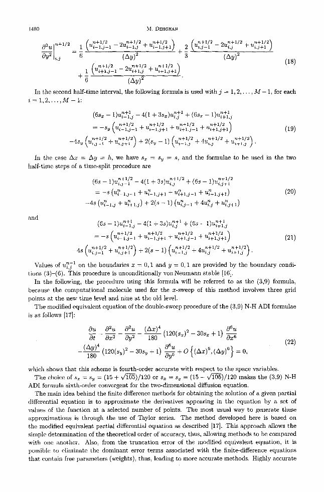
In the second half-time interval, the following formula is used with j = 1,2, . . . , M - 1, for each

i=1,2,...,M-1:

(6s, - l)u~-+ltj - 4(1 + 3S,)~~j+~ + (GS, - 1)~;‘;~

= -S 1/ ( %-1 j-l n+y2 + uy;y:1 + q$“1 + uyf:f$ ) (19)

-4s, (

u;;!{” + u;;;i2 , ) + 2(s, - 1) (U;J-;,$2 + 4U;;l’s + 1L;$i$2) .

In the case Ax = Ay = h, we have s, = sy = s, and the formulae to be used in the two

half-time steps of a time-split procedure are

(6s - l),;:{’ - 4(1 + 3s)~;;“~ + (6s - 1)~;;;~~

= -s (Cl,j-1 + 4-1,j+1 + G+l,j-1 + ur+l,j+l >

-4S (Ur-2-1.j + ur++l,j ) + 2(S - 1) (U$_i + 4ucj + UFj+*)

(6s - l)u;Trrj - 4(1 + 3s)~;;’ + (6s - l)u;;;,,

= -s Ur_l’,f$“i + zL;:ri;:i (

+ u;;i$“-i + U$i$$) (21)

-4s until2 ( z,3-i + $;{” ) + 2(s - 1) (U:_:t;s + 4U;;1’2 + u;$$ .

Values of u:T’ on the boundaries x = 0,l and y = 0,l are provided by the boundary condi-

tions (3)-(6). This procedure is unconditionally vonNeumann stable [16].

In the following, the procedure using this formula will be referred to a~ the (3,9) formula,

because the computational molecule used for the x-sweep of this method involves three grid

points at the new time level and nine at the old level. The modified equivalent equation of the double-sweep procedure of the (3,9) N-H AD1 formulae

is as follows [ 171:

au d2u d2u -- ---- at ax2 dy2

g (120(&)2 - 3os, + 1) g

(AY)~ -= (120(~,)~ - 30~~ + 1) $ + 0 {(AX)‘, (Ay)“} = 0, (22)

which shows that this scheme is fourth-order accurate with respect to the space variables.

The choice of s, = sy = (15 + &%)I120 or S, = sy = (15 - &%)/lZO makes the (3,9) N-H

ADI formula sixth-order convergent for the two-dimensional diffusion equation. The main idea behind the finite difference methods for obtaining the solution of a given partial

differential equation is to approximate the derivatives appearing in the equation by a set of

values of the function at a selected number of points. The most usual way to generate these approximations is through the use of Taylor series. The method developed here is based on

the modified equivalent partial differential equation as described [17]. This approach allows the

simple determination of the theoretical order of accuracy, thus, allowing methods to be compared

with one another. Also, from the truncation error of the modified equivalent equation, it is

possible to eliminate the dominant error terms associated with the finite-difference equations

that contain free parameters (weights), thus, leading to more accurate methods. Highly accurate

Two-Dimensional Parabolic Equation 1481

techniques can be found by incorporating weights into the discretisation process based on a

particular computational molecule. Values for these weights are chosen to eliminate as many

of the low-order error terms as possible in the modified equivalent partial differential equation

corresponding to the resulting finite difference equation. This is the origin of the (1/6,2/3,1/G)

weighting coefficients in formula (12)-(14).

2.2. The Standard (5,l) BTCS Method

The five-point BTCS (backward Euler) for solvin g the two-dimensional partial differential

equation (1) uses the following formula:

for i,j = 1,2 ,..., M- 1.

In the case s, = sY = s, we have

The computational molecule of this method involves five grid points at the new time level

and one at the old level. So, in the following this will be referred to as the (5,l) formula. This

technique is unconditionally stable [14].

The modified equivalent equation for this scheme is as follows [17]:

au 8% a*u -- --- a 8x2 dy2

_ @$ (1 + 64 !?& _ i$! (1 + Gs,) $ + 0 { (LLx)“. (AT,)“} = 0. (25)

So this scheme is second-order accurate with respect to the space variables. Note that there is

no set of values for which the method will be fourth-order accurate.

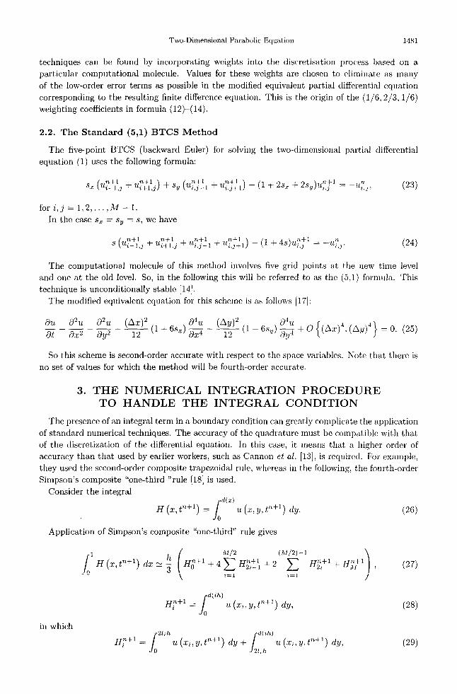
3. THE NUMERICAL INTEGRATION PROCEDURE TO HANDLE THE INTEGRAL CONDITION

The presence of an integral term in a boundary condition can greatly complicate the application

of standard numerical techniques. The accuracy of the quadrature must be compatible with that

of the discretization of the differential equation. In this case, it means that a higher order of

accuracy than that used by earlier workers, such as Cannon et al. [13], is requirccl. For example,

they used the second-order composite trapezoidal rule, whereas in the following, the fourth-order

Simpson’s composite “one-third “rule [18] is used.

Consider the integral

H (Xc, tn+l) = fz’ u (Ic, y, t”fl) dy. cw

Application of Simpson’s composite “one-third” rule gives

J 1

H (x, tn+‘) dz E ; ( AI/2 (Af/2)-1

If;+1 0

+4CHzn;t:+2 C ~,n,+l+~;;l

1

, (27) ?=l r=l

J d(lh)

H,n+’ = u (2% y, tn+y dy, (28) 0

in which 21,h

H,n+’ zz J d(lh)

u (.G,Yd ) n+l dyf J u (XI, Y, tnfl) &/, (29) 0 21,h

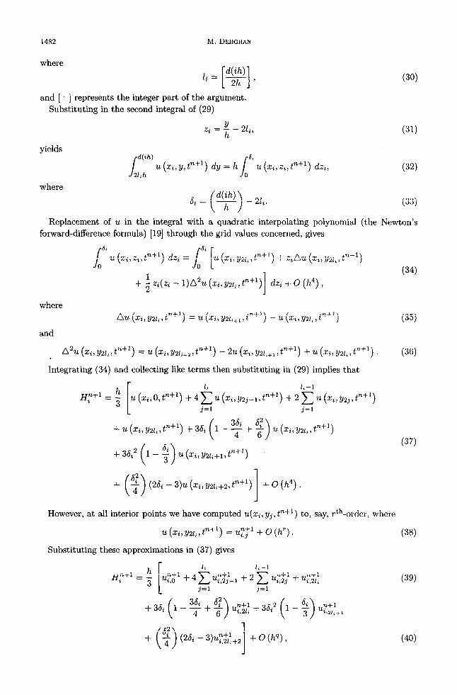
1482 M. DEHGHAN

where 1, = 4ih)

2

[ 1 2h’ and [ ] represents the integer part of the argument.

Substituting in the second integral of (29)

(36)

yields

where

.zi = f - 21i, (31)

J d(ih)

u (Xi, y, tn+l (32) 21;h

> ciy = h J” u (xi, zi,tn+l) dzi, 0

(33)

Replacement of ‘u. in the integral with a quadratic interpolating polynomial (the Newton’s

forward-difference formula) [19] through the grid values concerned, gives

J 6,

u (Xi, zi, tn+l 0

) dzi = I&i [u (Xi, y21, ,tn+‘) + zi,Au (xi, y21i 7 tn+‘)

)I (34)

dzi + 0 (h”) ,

where

and

Au (xi3 ?/21; 7 tn+‘) = u (xi7 Y21i+l, tn+‘) - U (xi, lJ2l,, tn+‘) (35)

, LJ2U (xi7 Y21; 7 tnfl) = U (xi7 Y21i+27 tn+‘) - 2U (xi, Y21;+17 tn+‘) + U (xi, Y21,1 t”+‘) . (36)

Integrating (34) and collecting like terms then substituting in (29) implies that

H,n+l = f u(2i,O,tn+l) +4+ci,y2j_,;t’+‘) +2~gu(%Y2j.i’i1)

2

+ u (G, Y21i, tn+‘) + 36, (

1 - $ + + >

u (Xi, y21;, tn+‘)

+ 36,s 1 - 2 ( 1

u (Xi, Y21,+1Jn+i)

(37)

+ (2& - 3)u (si, y/21;+2, tn+‘)

I

+ 0 (h4) .

However, at all interior points we have computed u(zi, Yj, tnfl) to, say, rth-order, where

u (zi,y21;,tn+1) = u;j” + 0 (h') . (38)

Substituting these approximations in (37) gives

H,Tz+’ = ; $0” j=l j=l

(39)

I

+ 0 (W, (49)

Two-Dimensional Parabolic Equation

where

q = min{r, 4).

Putting

V (P+l) = I1 H (R., tn+‘) kc,

and using the approximation

1483

(41)

(42)

V n+l =; AI/ 2 (M/2)-1

H;+l +4cH;lt_:+2 c H;;r+H;;r $-0(/i”), (43) i=l 1=1

then gives

h2 (M/2)-1

u ni-1 _ -- 9

.;,;l +4&;& + 2 c u;~++; + UT;; + Rn+’ + 0 (IL”). (44) i=l i=l

Note that 1 V n+l _ h

_- 3p

n+l s

lzc(.r) dx + R n+l + 0 (h”) ) 0

where R7’+l is the summation in un+’ excluding the values at the boundary 1/ = 0.

Since vn+l is an approximation to the left-hand side of (7), it follows that

(45)

pn+l ET

vn+l _ Rntl l (h/3) 1; ho(x) dx

+ 0 (izq-‘) , I ho(x) dn: # 0. 0

(45)

We assume that {uzj,pLn} are known, and we want to compute {u:~‘,/L~+~}. The itera-

tive algorithm is as follows: suppose the pth iteration {~:f”“, pn+“P} values are known at the

1~ + 1 level. If for a given tolerance E, Jmn+’ - v,“+‘.Pl 5 e, then we accept {~~fi’~,/~“+~~p}

as {p~::~, pun+l} at the time level IZ + 1. If not, then we use [13] the result to find a new estimate

for vn+l,P _ Rn+l,P

P n+l.p+l _

(h/3) J; ho(x) dx

+ 0 p-1) , (47)

from which the boundary values along y = 0 may be computed at time tn+i using (6).

This converts the two-dimensional diffusion with a nonclassical boundary condition to a bound-

ary value problem with an ordinary boundary condition.

As seen above, the order of convergence of p depends on two things: first, the order of the finite-

difference formula used at interior gridpoints, and second, the order of the numerical quadrature

used to approximately evaluate (7). For example, if u ntl is evaluated using a fourth-order

formula, when q = 4, p n-t1 is only third-order convergent. If un+r is found at interior points by

a second formula when q = 2, then pnfl is only first-order convergent.

4. APPLICATIONS

Two-dimensional parabolic equations with an integral condition involving specification of mass

occurs in a number of practical problems. For example, it is often feasible to utilize absorption

of light at certain frequencies by a chemical in solution in order to measure its concentration.

However, due to the finite size of the light beam and the summation character of the clectjronics,

any such measurement of a chemical during a diffusion process amounts to a quadrat,ure of the

variable concentration over the spatial region through which the light beam passes. This yields

a measurement of the total mass of the chemical in that spatial region. Moreover, in order to

smooth the data, the resulting spatial quadrature can be integrated with respect to time. In many

chemical situations involving the determination of unknown diffusivities and unknown kinetic rate constants, this kind of data is all that can be obtained. Interested readers can see [1,5-7,10,11]

for more information.

1484 M. DEHGHAN

5. NUMERICAL TEST

Two problems with exact known solutions are now used to test the method developed in this

report.

5.1. Test 1

Consider (l)-( 7) with

fb, Y) = exdz + Y),

sob, t) = exp(y + 2% gl(y,t) = exp(l + Y + 2%

ho(x) = expb), hr(z:, t) = exp(1 + 2 + 2t),

cl(t) = exp(2t),

m(t) = (exp(l) - 1)2 exp(2t),

d(X) = X(1 -z),

(48) (49) (50)

(51)

(52)

(53)

(54)

(55)

for which the exact solution is

u(z, y, t) = exp(z + y + 2t). (56)

Consider (l)-(7) with the functions f, ho, hr, ga,gr, m, ,LL, and d as defined by (48)-(55). The

exact solution for this problem is (56).

Using the (3,9) N-H AD1 method and the standard BTCS of [13] and defining m(t) as in (54)

and excluding (53) and using (55), the results for ucj with h = 0.02, s = l/2 at T = 1.0, are

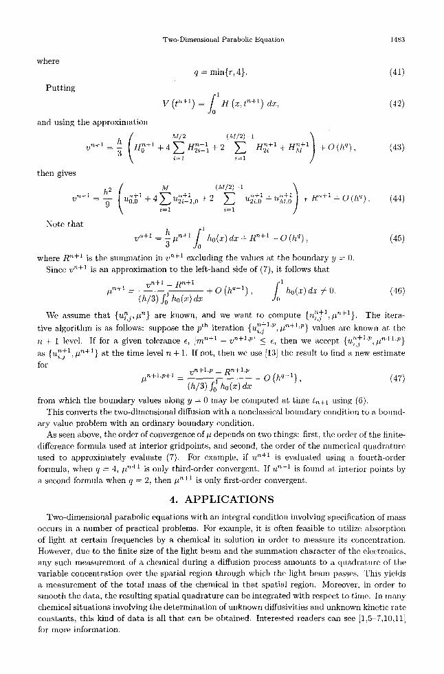
obtained and shown in Table 1. Note that the results obtained when using the (3,9) N-H ADI

are about 100 times more accurate than those obtained when using the standard BTCS method.

Table 1. Results for u from Test 1 with T = 1.0, h = 0.02, s = l/2.

T

Standard-BTCS (3,9) N-H ADI

X Y Exact u Error Error

0.1 0.2

0.3

0.4

0.5

0.6

0.7

0.8

0.9

0.1

0.2

0.3

0.4

0.5

0.6

0.7

0.8

0.9 L

9.025013 2.1 x 10-d -6.6 x 10-s

11.023176 2.2 x 10-d -2.0 x 10-s

13.463738 2.3 x 1O-4 -3.5 x 10-s

16.444647 2.0 x 10-d -4.8 x lo-+

20.905243 2.3 x 1O-4 -5.7 x 10-6

24.532530 2.4 x 1O-4 -6.0 x lo-+

29.964100 2.6 x 1O-4 -5.4 x 10-s

36.598234 2.5 x 1O-4 -3.9 x 10-e

40.447304 2.4 x 1O-4 -1.8 x lO+

When the absolute value of the error

(57)

at the point (0.5,0.5) at time T = 1.0 was graphed against h on a logarithmic scale for various values of s, it was found that the slopes of lines were always close to 2 for the BTCS formula, and

they were close to 4 for the (3,9) N-H AD1 formula. These results reflect the orders of convergence

referred to in Section 2.

Two-Dimensional Parabolic Equation 1485

The interesting feature of the results was that the maximum discretisation error produced by

the (3,9) N-H AD1 scheme was smaller than the minimum discretisation error obtained when

using the standard BTCS method.

The CPU time was 2128.5 set for the (5,l) BTCS technique, while it was 259.7sec for the (3,9)

N-H AD1 finite difference formula.

The results for p with h = 0.02, s = l/2, using the BTCS method and the (3,9) N-H AD1

method to solve the example nonclassic boundary value problem are shown in Table 2. Note that

the solutions obtained when using the BTCS method are generally less accurate, by about two

orders of accuracy, than those obtained using the (3,9) N-H AD1 scheme.

Table 2. Results for p from Test 1 with h = 0.02, s = l/2.

-

- t

- 0.1

0.2

0.3

0.4

0.5

0.6

0.7

0.8

0.9

1.0 -

Exact p Error Error

1.221403 -1.3 x 10-s -2.5 x 1O-5

1.491825 -1.6 x 1O-3 -2.3 x 10-a

1.822119 -2.0 x 10-a -2.4 x 1O-5

2.225541 -2.4 x 1O-3 -2.6 x 1O-5

2.718282 -3.0 x 10-s -2.7 x lo-”

3.320117 -3.6 x 1O-3 -3.5 x 10-a

4.055200 -4.5 x 10-s -3.4 x 10-a

4.953032 -5.4 x 10-s -2.9 x 1O-5

6.049647 -6.6 x 10-s -2.9 x 1O-5

7.389056 -8.1 x 1O-3 -2.8 x 1O-5

Standard-BTCS (3,Q) N-H ADI

When the absolute value of the error

en = p(nk) - pn, (58)

at the point (0.5,0.5) was graphed against h on a logarithmic scale for various values of s, it was

found that the slopes of lines were always close to 1 for the BTCS finite difference scheme, but

they were close to 3 for the (3,9) N-H AD1 finite difference formula. These results again reflect

the orders of convergence referred to earlier.

5.2. Test 2

Consider (l)-(7) with

fh 9) = (1 - Y) exr-+),

s0(y, t) = (1 - y) w(t), sl(Y, t) = (1 - Y) exp(l + t),

ho(x) = exp(~c), hl(T t) = 0,

At) = exd% m(t) = (22 - 8exp(l)) exp(t),

d(z) = X(1 - X),

(59) (60) (61) (62) (63)

(64)

(85)

(88)

for which the exact solution is

~(2, y, t) = (1 - y) exp(z + t). (87)

1486 M. DEHGHAN

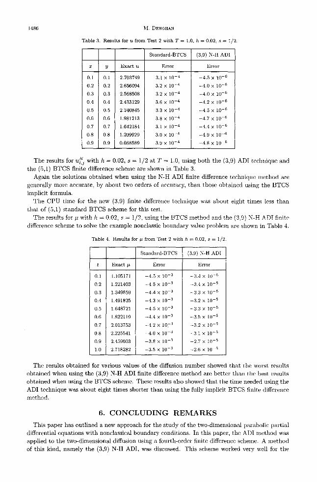
Table 3. Results for ‘11 from Test 2 with 2’ = 1.0, II = 0.02, s = l/2

-

- 2

-

0.1

0.2

0.3

0.4

0.5

0.6

0.7

0.8

0.9 -

Y

0.1

0.2

0.3

0.4

0.5

0.6

0.7

0.8

0.9

Standard-BTCS (3,9) N-H ADI

Exact u Error Error

2.703749 3.1 x 10-d -4.5 x 10-G

2.656094 3.2 x 1O-4 -4.0 x 10-s

2.568508 3.2 x 1O-4 -4.0 x 10-s

2.433129 3.6 x 1O-4 -4.2 x lo@

2.240845 3.3 x 10-d -4.5 x 10-s

1.981213 3.8 x 1O-4 -4.7 x 10-s

1.642184 3.1 x 10-4 -4.4 x 10-s

1.209929 3.0 x 10-d -4.9 x 10-s

0.668589 3.9 x 10-d -4.8 x lo-”

The results for u& with h = 0.02, s = l/2 at T = 1.0, using both the (3,9) AD1 technique and

the (5,l) BTCS finite difference scheme are shown in Table 3.

Again the solutions obtained when using the N-H AD1 finite difference technique method are

generally more accurate, by about two orders of accuracy, than those obtained using the BTCS

implicit formula.

The CPU time for the new (3,9) finite difference technique was about eight times less than

that of (5,l) standard BTCS scheme for this test.

The results for p with h = 0.02, s = l/2, using the BTCS method and the (3,9) N-H AD1 finite

difference scheme to solve the example nonclassic boundary value problem are shown in Table 4.

Table 4. Results for p from Test 2 with h = 0.02, s = l/2

Standard-BTCS (3,9) N-H ADI

t Exact p Error Error

0.1 1.105171 -4.5 x 10-S -3.4 x 10-S

0.2 1.221403 -4.5 x 10-s -3.4 x 10-S

0.3 1.349859 -4.4 x 10-S -3.3 x 10-s

0.4 1.491825 -4.3 x 10-S -3.2 x 1O-5

0.5 1.648721 -4.5 x 10-s -3.3 x 10-s

0.6 1.822119 -4.4 x 10-S -3.5 x lo-”

0.7 2.013753 -4.2 x 1O-3 -3.2 x lo-”

0.8 2.225541 -4.0 x 10-S -3.1 x 10-S

0.9 2.459603 -3.8 x 1O-3 -2.7 x IO-”

1.0 2.718282 -3.5 x 10-S -2.6 x lo-”

The results obtained for various values of the diffusion number showed that the worst results

obtained when using the (3,9) N-H AD1 finite difference method are better than the best results

obtained when using the BTCS scheme. These results also showed that the time needed using the

AD1 technique was about eight times shorter than using the fully implicit BTCS finite difference

method.

6. CONCLUDING REMARKS

This paper has outlined a new approach for the study of the two-dimensional parabolic partial

differential equations with nonclassical boundary conditions. In this paper, the AD1 method was

applied to the two-dimensional diffusion using a fourth-order finite difference scheme. A method

of this kind, namely the (3,9) N-H ADI, was discussed. This scheme worked very well for the

Two-Dimensional Parabolic Equation 1487

two-dimensional diffusion equation with a nonclassical boundary condition, because of its high

accuracy. The AD1 scheme described in this report is unconditionally stable and solvable. A

comparison with the standard fully implicit scheme of [13] for the two-dimensional parabolic

partial differential equation with an integral condition replacing one boundary condition clearly

demonstrates the new technique to be computationally superior. In the standard fully implicit

finite difference scheme, five unknown values at the time tn+l are involved in the difference

equation. Hence, this method requires the solution of a large number of simultaneous linear

algebraic equations at all grid points at each time step. The huge amount of CPU time which is

needed to solve the resulting wide banded matrix makes this method impractical. In the standard

fully explicit method, only one unknown is involved in the finite difference formula. Therefore,

all the values at time tn+l can be calculated point by point. A noticeable behaviour of the

standard fully explicit finite difference method is the restriction of the size of the time step due

to stability requirements. This restriction necessitates extremely small values for the time step

size. This limitation is removed when the standard fully implicit finite difference scheme is used.

A comparison with the standard fully implicit scheme for the numerical solution of nonclassical

boundary value problems shows the standard fully implicit method, even though it ha.s extended

range of stability, uses large central processor times. So the need to develop AD1 methods is

clear. The main advantage of AD1 finite difference techniques is that the bandwidth of the

sets of equations is a fixed small number that depends only on the nature of the computational

stencil. This allows the use of very efficient and very fast techniques for solving the resulting

tridiagonal systems of linear algebraic equations such as the Thomas algorithm. The (3,9) AD1

finite difference scheme developed in this report is very easy to implement for similar three-

dimensional problems, but it may be more difficult when dealing with the standard fully implicit

scheme.

REFERENCES

1. J.R. Cannon and J. vanderHoek, Diffusion subject to the specification of mass, J. Math. Anal. Appl. 115, 517-529, (1986).

2. J.R. Cannon, S. Prez-Esteva and J. vander Hoek, A Galerkin procedure for the diffusion equation subject to the specification of mass, SIAM. J. Num. Anal. 24, 499-515, (1987).

3. J.R. Cannon and A. Matheson, On the numerical solution of diffusion subject to the specification of mass, Intern. J. Engng. Sci. 31, 347-355, (1993).

4. J.R. Cannon, Y. Lin and S. Wang, An implicit finite difference scheme for the diffusion equation subject to mass specification, Intern. J. Engng. Sci. 28, 573-578, (1990).

5. V. Cpasso and K. Kunisch, A reaction-diffusion system arising in modeling man-environment diseases. Quart. Appl. Math. 46, 431-449, (1988).

6. Y.S. Choi and K.Y. Chan, A parabolic equation with nonlocal boundary conditions arising from electrochem- istry, Nonlinear Analysis, Theory, Methods, and Applications 18 (4), 317-331, (1992).

7. W.A. Day, A decreasing property of solutions of a parabolic equation with applications in thermoelasticity and other theories, Quart. Appl. Math. 41, 475-486, (1983).

8. M. Dehghan, A finite difference method for a non-local boundary value problem for ‘L-dimensional heat equation, Appl. Math. Comput. 112 (l), 133-142, (2000).

9. G. Ekolin, Finite difference methods for a non-local boundary value problem for the heat equation, BIT 31 (2), 245-255, (1991).

10. P. Marcati, Some considerations on the mathematical approach to nonlinear age dependent population dy- namics, Computers Moth. Applic. 9 (3), 361-370, (1983).

11. S. Wang, A numerical method for the heat conduction subject to moving boundary energy specification, Numerical Heat lPransfer 130, 35-38, (1990).

12. S. Wang and Y. Lin, A numerical method for the diffusion equation with non-local boundary specifications, Intern. J. Engng. Sci. 28, 543-546, (1991).

13. J.R. Cannon, Y. Lin and A. Matheson, The solution of the diffusion equation subject to specification of mass. Appl. Anal. 50 (2), l-11, (1993).

14. A.R. Mitchell and D.F. Griffiths, The Finite Di%ference Methods in Partial Difierential Equations, Wiley, (1980).

15. B.J. Noye and K.J. Hayman, LOD and ADI methods for the two-dimensional diffusion equation, Intern. J. Comput. Math. 51, 215-228, (1994).

16. N.I. Yurchuk, Mixed problem with an integral condition for certain parabolic equations, DZfl. Eqns. 22, 1457-1463, (1986).

1488 M. DEHCHAN

17. R.F. Warming and B.J. Hyett, The modified equation approach to the stability and accuracy analysis of finite difference methods, Journal of Computational Physics 14 (2), 159-179, (1974).

18. C.F. Gerald and P.O. Wheatley, Applied Numerical Analysis, Fifth Edition, Addison-Wesley, California, (1994).

19. S. Wang and Y. Lin, A finite difference solution to an inverse problem determining a control function in a parabolic partial differential equation, Inverse Problems 5, 631-640, (1989).