A Natural Representation of Functions for ExactLearningBenedict Irwin  ( ben@optibrium.com )

Optibrium Ltd. https://orcid.org/0000-0001-5102-7439

Article

Keywords: exact learning method, mathematical tools

Posted Date: February 4th, 2021

DOI: https://doi.org/10.21203/rs.3.rs-149856/v1

License: This work is licensed under a Creative Commons Attribution 4.0 International License.  Read Full License

A Natural Representation of Functions for Exact Learning

Benedict W. J. Irwin*1,2

1Theory of Condensed Matter, Cavendish Laboratories, University of Cambridge,

Cambridge, United Kingdom

2Optibrium Ltd., F5-6 Blenheim House, Cambridge Innovation Park, Denny End Road,

Cambridge, CB25 9PB, United Kingdom

1ben.irwin@optibrium.com

January 1, 2021

Abstract

We present a collection of mathematical tools and emphasise a fundamental representation of ana-

lytic functions. Connecting these concepts leads to a framework for ‘exact learning’, where an unknown

numeric distribution could in principle be assigned an exact mathematical description. This is a new

perspective on machine learning with potential applications in all domains of the mathematical sciences

and the generalised representations presented here have not yet been widely considered in the context of

machine learning and data analysis. The moments of a multivariate function or distribution are extracted

using a Mellin transform and the generalised form of the coefficients is trained assuming a highly gener-

alised Mellin-Barnes integral representation. The fit functions use many fewer parameters contemporary

machine learning methods and any implementation that connects these concepts successfully will likely

carry across to non-exact problems and provide approximate solutions. We compare the equations for the

exact learning method with those for a neural network which leads to a new perspective on understanding

what a neural network may be learning and how to interpret the parameters of those networks.

1 Introduction

Machine learning (ML) is - simplistically speaking - a form of function fitting and ML methods often try to

recreate a set of training observations by fitting a function to - or ‘learning from’ - example data points. For

a given problem, the most appropriate ML method to use will depend on the application. In general, great

1

success has been seen using this kind of methodology on a range of problems across all domains of science

and industry. Most current ML methods recreate the input data by an approximation or interpolation of

a restricted sample of training points. Any learning that happens by these methods is then also in some

sense restricted or limited to the domain of the training set or conditions in which the data were collected.

The form chosen to fit the data - the model - is usually selected for convenience, convergence properties,

speed, or simplicity and interpretability and the coefficients/weights/parameters learned are likely to be

somewhat arbitrary, not necessarily represent anything fundamental, and become much harder to interpret

as the method gets increasingly complex [1]. In order to reach these high precision approximations, many

parameters are used, sometimes millions or billions of parameters, especially in the case of neural networks

and deep learning methods [2].

The trained model from the above methods is unlikely to be ‘physically meaningful’, by which we mean

- unlikely to lead to transparent and understandable insight that can be condensed down into a human

readable form. The outputs of the model can still be very useful, for example to interpolate between known

physical results [3], but the model itself is not necessarily fundamental. This makes it hard for current ML

methods to assist in the collection of fundamental things, or ‘natural facts’, specifically mathematical facts.

True learning - in a mathematical sense - is timeless. If an exact solution to a problem exists - for example

a solution to a particular differential equation - this solution is a permanent solution which can be defined,

collected, and documented in a human readable form1. If the same equation is written years in the future the

same solution will apply. Learning such a fact correctly would then be an example of ‘exact learning ’. This

notion is more relevant to problems from mathematics and physics where there is an unchanging ‘ground

truth’ defined by nature, for example laws of physics.

We will consider how in a broad sense ‘machine-learning-like-techniques’ (i.e. advanced function fitting),

can help with these ‘exact learning’ type problems. Specifically for this work, the problem description is:

A) ‘Given a high precision numeric output of an unknown multivariate function or distribu-

tion write the ‘human readable equation’ for that function as output, where it is possible

to do so.”

The concession we are willing to take on this quite general goal is:

B) ‘Given a high precision numeric output of an unknown multivariate distribution write

the unique fingerprint of the distribution.’

1Subject to the language required to document the function existing.

2

The key change in goal B) is the introduction of a ‘fingerprint ’ of an arbitrary function as a well behaved

and meaningful intermediate that can identify a distribution 2. The word fingerprint is local to this text and

should not be considered a general term. The goals A) and B) can be seen as reverse engineering processes

for functions. It might be helpful to first consider the analogy of reverse engineering for a simpler object

such as a number, something that is performed by tools such as Simon Plouffe’s ‘inverse symbolic calculator’

[4] and other ‘inverse equation solvers’ [5]. In these tools a user can enter a high precision number - e.g.

14.687633495788080676 - and the algorithm would return a plausible closed form solution - e.g. π2 + e√π.

Once the user has the solution, the hope is that a human expert could use that extra information to come

up with further insights which would assist in the scientific understanding of both the solution and problem.

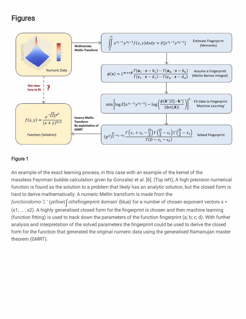
Figure 1 depicts an overview of the ‘exact learning’ procedure for a function. Throughout this work

we cover the necessary tools to understand the steps in the blue boxes on the right-hand side of this fig-

ure. Goal A) corresponds to the bottom left box, and goal B) is the bottom right box. The numeric data

are collected from a natural source such as a very high-quality experiment, but more likely a numerical

solution to a computational problem, or equation, or simulation. The solution is numerically transformed

to ‘fingerprint space’ (blue) by using an integral transform. The regularity of the representation of many

analytic functions in this space assists with the fitting of the ‘fingerprint’ using machine learning techniques

to an assumed, highly generalised form. To get back to the mathematical expression of the solved func-

tion an inverse transformation is taken from the fingerprint space to the function space. For examples of

problems that might be interesting to solve using this method, please refer to the supplementary information.

1.1 Brief Disclaimer

This intends to be a foundational paper that sparks an idea and lays the concepts on the table but stops

short of connecting them together. This is to avoid invoking (an explanation of) the technical requirements

that are needed for an implementation. Many of the tools described here are treated in a highly rigorous

mathematical way in the literature. While this is necessary for the correctness of the underlying mathe-

matics, we feel it reduces the accessibility of the concepts, innovation, and creativity. We will introduce the

necessary fundamentals with a high level overview and point to more technical references where possible.

There are a number of limitations and potential ‘engineering problems’ that may need to be overcome

2We have focused on distributions for the time being for simplicity, but extensions to this method will cover functions whichare not bound at infinity

3

Figure 1: An example of the exact learning process, in this case with an example of the kernel of the masslessFeynman bubble calculation given by Gonzalez et al. [6]. (Top left), A high precision numerical functionis found as the solution to a problem that likely has an analytic solution, but the closed form is hard toderive mathematically. A numeric Mellin transform is made from the ‘function domain’ (yellow) into the‘fingerprint domain’ (blue) for a number of chosen exponent vectors s = (s1, · · · , s2). A highly generalisedclosed form for the fingerprint is chosen and then machine learning (function fitting) is used to track downthe parameters of the function fingerprint (a,b, c,d). With further analysis and interpretation of the solvedparameters the fingerprint could be used to derive the closed form for the function that generated the originalnumeric data using the generalised Ramanujan master theorem (GMRT).

when training networks that are constructed using these concepts introduced below. For a further discussion

of limitations please see the supplementary information. Further work is undoubtedly required to overcome

these issues and some of these are discussed with the conclusions. The key message of this work is: ‘Let us

turn our attention to a special hierarchy of functions and associated methods while keeping machine learning

in mind. What algorithms can be developed from this?’.

2 Background and Method

We will go through the background theory and arrangement of concepts required to exactly learn functional

forms from high-quality numeric data. As with other types of machine learning, fitting and optimisation

problems, it is convenient to define a loss function that should be minimised to solve the problem [7]. If

this loss function takes a standard form, there are many available minimisation methods, for example using

the gradient of the loss function with respect to network parameters [8]. The training process for a method

4

built using the loss function would then resemble backpropagation for a (deep) neural network [9, 2] and

completed algorithm is more likely to be implementable with existing software packages such as TensorFlow

[10] and PyTorch [11]. Other learning strategies may prove more efficient or robust [12].

For the time being, this conceptual loss function will be the squared difference of the ‘experimental

fingerprint’ of the numerical solution, after the transformation into fingerprint space, and the ‘theoretical

fingerprint’ i.e the model we are trying to fit to the data. We then answer the questions: ‘What is the

fingerprint of a function?’ and ‘How do we measure this fingerprint both experimentally and theoretically?’.

The fingerprint we choose in this work is the so-called Mellin transform of a function or distribution [13].

To understand the rationale behind choice this we first explain a pattern in the generalised representation

of analytic functions which we believe to be fundamental.

2.1 Nature’s Language for Analytic Functions

Many different types of mathematical function are used across the mathematical sciences. Because the lan-

guage of mathematics is an ad hoc set of notation which has evolved with time it can be hard to keep a

sense of order on named functions. Many people will be familiar with the functions exp(x) and log(x), or

trigonometric functions such as sin(x). In engineering and physics additional special functions are developed

for convenience, e.g. Bessel functions which can relate to cylindrical harmonics, along with various special

(orthogonal) polynomials and these functions and identities appear in large catalogues [14].

The subset of analytic functions have power series expansions which allow easier comparison between

functions. Many of these series expansions can represented in terms of so-called hypergeometric series.

A a core-component of this description is the gamma function

Γ(s) =

∫∞

0

xs−1e−xdx, (1)

which is the continuous analogue to the factorial function n! [13, 14]. The gamma function will be pivotal

for our definition of a function’s fingerprint. We also note that s should generally be considered a complex

number.

Functions that can be described as a hypergeometric series can be represented as a limiting case of the

so-called hypergeometric function which can be written in terms of ratios of gamma functions. We can

5

write the hypergeometric function (with a negative argument) as

2F1(a, b; c;−x) =∞∑

s=0

(−1)s

s!

Γ(c)Γ(a+ s)Γ(b+ s)

Γ(a)Γ(b)Γ(c+ s)xs, (2)

where the notable component is the collection of gamma functions in the series. In this work we define the

fingerprint of the hypergeometric function as the so-called Mellin transform [13] of the function,

M [2F1(a, b; c;−x)] (s) =Γ(c)Γ(a− s)Γ(b− s)Γ(s)

Γ(a)Γ(b)Γ(c− s)︸ ︷︷ ︸

fingerprint

, (3)

which is related to the series coefficients in equation 2. For a large set of analytic functions used in science and

mathematics, the fingerprint is described as a product of gamma functions and their reciprocals.

This scratches the surface of the fundamental pattern we will exploit to allow machine learning methods to

adapt to unknown functions. For more examples of the Mellin transform and for a list of example functions

from science and mathematics that can be described by hypergeometric series and increasingly generalised

series see the supplementary information.

Many analytic functions cannot be described by the simple hypergeometric series in equation 2 [15].

There are further extensions to the series definition which begin to describe these additional functions. This

process of generalisation has iterated numerous times over the course of history [16, 17, 18, 15], each time

capturing successively more of the functions which are not described by the previous iterations. It is this

neat and hierarchical way of organising this huge space of functions which we will use as a language for ‘ex-

act learning’. The latest and more complex iterations have provided functions which can describe complex

phenomena from physics such as the free energy of a Gaussian model of phase transition [15]. We will briefly

describe the language used to define these highly generalised functions.

2.1.1 A Language to Define Analytic Functions

The Mellin transform converts a function into its fingerprint and the inverse Mellin transform transforms

the fingerprint into the function. The inverse Mellin transform is defined by a contour integral, that uses

the residue theorem to recreate the series expansion of the function [13, 19]. The more generalised functions

considered in this work are defined in terms of this contour integral [15, 20, 21], which is often called a

Mellin-Barnes integral [19]. For the hypergeometric function (Equation 2) a corresponding definition

6

through a Mellin-Barnes integral is

2F1(a, b; c;−x) =1

2πi

∫ i∞

−i∞

Γ(c)Γ(a+ s)Γ(b+ s)Γ(−s)Γ(a)Γ(b)Γ(c+ s)

xs ds. (4)

there are technical reasons for this choice of languge over a simpler series representation. For example a

different choice of contour can lead to different representations of a series [15], other methods to compute

Mellin transforms find multiple ways of getting to the same answer [6]. We will not dive into the technical

details, but present equation 4 to observe that the contents of this Mellin-Barnes integral is simply the

fingerprint, with a change of sign s→ −s.

2.1.2 A Fundamental Duality

The duality between a function and its Mellin transform has proved useful in numerous advanced mathemat-

ical applications including quantum field theory [6], cosmology [22], and string theory [23]. Schwinger and

Feynman parametrisation for the calculation of loop integrals from Feynman diagrams make heavy use of

Mellin transforms [24] and the resulting ‘Mellin space’ has been viewed as a ‘natural language’ for attempts

to align quantum gravity and quantum field theory in Ads/CFT methods [25]. It is possible to convert the

regular Fourier duality3 of quantum mechanics into a ‘Mellin duality’, which leads to wavefunctions asso-

ciated with the zeta functions commonly seen in number theory [26]. Aspects of particle physics have also

previously been noted in the analytically continued coefficient space of zeta type functions [27]. Therefore, it

is not out of the question that the Mellin transform representation of the ‘fingerprint’ also be a natural choice

for exact learning. This representation is the frame in which functions are defined by their zeroes and poles, in

the same way that many properties of prime numbers are defined by the zeroes of the Riemann zeta function.

There is a simple relationship between the Fourier transform F , the (two-sided) Laplace transform L

and the Mellin transform M for a function f . Namely, the Mellin transform of a function M[f(x)](s) is

the same as the Laplace transform of the same function with negative exponential argument, L[f(e−x)](s),

which is related to the Fourier transform as F [f(e−x)](−is), and likewise the Fourier transform of a function

F [f(x)](−s), relates to L[f(x)](−is) and to M[f(− lnx)](−is).

Dualities in these other two transform spaces have been known for a long time to statistics including the

relationship between the characteristic function and the distribution in terms of a Fourier transform [28],

and the moment generating function and a distribution in terms of the Laplace transform [29]. However, in

3Position and momentum, and time and frequency form conjugate pairs of variables.

7

terms of fingerprint equivalents, Laplace and Fourier transforms do not display the regularity of the Mellin

transforms in terms of patterns of gamma functions alluded to in the above sections. This can be seen

by reviewing extensive tables of each type of transform [30]. Many of the identities for Fourier transforms

relate to trigonometric functions and Bessel functions and many of the Laplace transform identities relate

to algebraic expresions and exponential terms. Both Fourier and Laplace transforms make extensive use of

special functions such as error functions, exponential integrals and more complicated, niche special functions.

On the other hand, the Mellin transform identities mostly revolve around gamma functions and polygamma

functions, hypergeometric functions and terms such as beta functions and other shorthands which can actu-

ally be expressed again as gamma functions e.g. π csc(πs) = Γ(s)Γ(1− s). Loosly speaking, these ‘elements’

that form the Mellin transforms all have something to do with gamma functions.

The Mellin transform connects a distribution to its moments, and learning using moments has been

considered before, including the generalised method of moments [31]. These methods do not consider an

underlying structure to the moment space, but only that estimators of statistical quantities phrased in

terms of moments can be advantageous. In general, integral transforms link strongly to inner products in

vector spaces and further work would be required to establish a deep connection between ‘exact learning’

as presented here to well studied mathematical formalisms such as reproducing kernel Hilbert spaces [32],

specifically those with a monomial kernel xs as seen in the Mellin transform. Further much deeper mathe-

matical connections are apparent, including the generalisation of the Mellin transform in terms of a Gelfand

transform, or the analogies between hypergeometric functions and ‘basic hypergeometric’, ‘q-hypergeometric’

and elliptic variants [33].

To summarise, the Mellin transform can mediate a duality between a distribution and its moments, or

an analytic function and its coefficients in the same way that a Fourier transform can mediate a duality

between time and frequency, or position and momentum. In terms of function fitting, an analytic function

represented as a power series has infinite coefficients to fit, however, by applying the Mellin transform the

coefficients are not trained individually but the whole set of coefficients are trained simultaneously.

2.1.3 Generalisation of Generalised Functions

For the generalised functions beyond the hypergeometric function, the product of gamma functions that forms

the fingerprint begins to have numerous terms and it is helpful to define a concise notation for a ‘product

gamma’ operation, Ξ[·], which flattens a vector or matrix and takes a product of the gamma function over

the elements. The use of this custom operation will make the pattern between the functions much easier

8

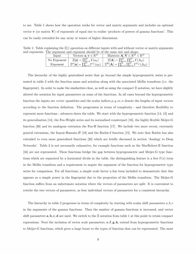
to see. Table 1 shows how the operation works for vector and matrix arguments and includes an optional

vector v (or matrix V) of exponents of equal size to realise ‘products of powers of gamma functions’. This

can be easily extended for any array or tensor of higher dimensions.

Table 1: Table explaining the Ξ[·] operation on different inputs with and without vector or matrix argumentsand exponents. The argument and exponent should be of the same size and shape.

Input Vectors a,v ∈ RD Matrices A,V ∈ R

D × RD

No Exponent Ξ[a] =∏D

k=1 Γ(ak) Ξ[A] =∏D

k=1

∏Dl=1 Γ(Akl)

Exponent Ξv[a] =∏D

k=1 Γvk(ak) ΞV[A] =

∏Dk=1

∏Dl=1 Γ

Vkl(Akl)

The hierarchy of the highly generalised series that go beyond the simple hypergeometric series is pre-

sented in table 2 with the function name and notation along with the associated Mellin transform (i.e. the

fingerprint). In order to make the similarities clear, as well as using the compact Ξ notation, we have slightly

altered the notation for input parameters on some of the functions. In all cases beyond the hypergeometric

function the inputs are vector quantities and the scalar indices p, q,m, n denote the lengths of input vectors

according to the function definition. The progression in terms of complexity - and therefore flexibility to

represent more functions - advances down the table. We start with the hypergeometric function [14, 13] and

its generalisation [14], the Fox-Wright series and its normalised counterpart [16], the highly flexible Meijer-G

function [30] and its analogous extension the Fox-H function [17]. We include two more recent, extremely

general extensions, the Inayat-Hussain-H [18] and the Rathie-I function [15]. We note that Rathie has also

extended to even more generalised functions [20] which are briefly discussed in section ‘Analogy to Deep

Networks’. Table 2 is not necessarily exhaustive, for example functions such as the MacRobert-E function

[34] are not represented. These functions bridge the gap between hypergeometric and Meijer-G type func-

tions which are separated by a horizontal divide in the table, the distinguishing feature is a free Γ(s) term

in the Mellin transform and a requirement to negate the argument of the function for hypergeometric type

series for comparison. For all functions, a simple scale factor η has been included to demonstrate that this

appears as a simple power in the fingerprint due to the properties of the Mellin transform. The Meijer-G

function suffers from an unfortunate notation where the vectors of parameters are split. It is convenient to

rewrite the two vectors of parameters, as four individual vectors of parameters for a consistent hierarchy.

The hierarchy in table 2 progresses in terms of complexity by starting with scalar shift parameters a, b, c

in the arguments of the gamma functions. Then the number of gamma functions is increased, and vector

shift parameters a,b, c,d are used. We switch to the Ξ notation from table 1 at this point to retain compact

expressions. Next the inclusion of vector scale parameters, e, f ,g,h, extend from hypergeometric functions

to Meijer-G functions, which gives a large boost to the types of function that can be represented. The most

9

Table 2: A table of generalised special functions and their Mellin transforms. Small bold letters are vectorsof parameters where a,b, c,d are shift factors, e, f ,g,h are scale factors and i, j,k, l are exponents for thegamma functions, 1 represents a vector containing only 1’s. Complexity increases down the table which issplit into an upper part for hypergeometric functions and a lower part for Meijer-G like functions.

FunctionName

f(x) Fingerprintϕ(s) = M[f(x)](s)

Ref.

Hypergeometric 2F1

(a, b

c

∣∣∣∣− ηx

)

η−s Γ(c)Γ(a−s)Γ(b−s)Γ(a)Γ(b)Γ(c−s) Γ(s) [14, 30]

GeneralisedHypergeometric

pFq

(a

b

∣∣∣∣− ηx

)

η−s Ξ[b]Ξ[a−s1]Ξ[a]Ξ[b−s1]Γ(s) [14, 30]

Fox-Wright-Ψ pΨq

[a, e

b, f

∣∣∣∣− ηx

]

η−s Ξ[a−se]Ξ[b−sf ]Γ(s) [16]

Fox-Wright-Ψ∗

pΨq

[a, e

b, f

∣∣∣∣− ηx

]

η−s Ξ[b]Ξ[a−se]Ξ[a]Ξ[b−sf ]Γ(s) [16]

Meijer-G Gm,np,q

(a,b

c,d

∣∣∣∣ηx

)

η−s Ξ[1−a−s1]Ξ[c+s1]Ξ[1−d−s1]Ξ[b+s1] [30, 19]

Fox-H H m,np,q

[a,b, e, f

c,d,g,h

∣∣∣∣ηx

]

η−s Ξ[1−a−se]Ξ[c+sg]Ξ[1−d−sh]Ξ[b+sf ] [17, 21]

Inayat-Hussain-H

H m,np,q

[a,b, e, f , i

c,d,g,h, l

∣∣∣∣ηx

]

η−s Ξi[1−a−se]Ξ[c+sg]Ξl[1−d−sh]Ξ[b+sf ]

[18]

Rathie-I I m,np,q

[a,b, e, f , i, j

c,d,g,h,k, l

∣∣∣∣ηx

]

η−s Ξi[1−a−se]Ξk[c+sg]Ξl[1−d−sh]Ξj[b+sf ]

[15]

general functions come from adding vector power parameters i, j,k, l, which begin to describe non-trivial

physical and number theoretic functions [15].

All of the functions in table 2 assume an analytic series expansion. For certain sets of parameters, the

series expansions for many commonly used functions in physics and mathematics can arise. A small list is

given in the supplementary information. Many of these functions have constraints on the combinations of

arguments that can be used. For the sake of focus and scope in this text we will not mention any regions of

convergence or the necessary analytic continuations in the following sections, but these should be considered

carefully when such equations are implemented numerically and solved fingerprints are interpreted. A careful

treatment is given by the following references [35, 23, 36] as well as the reference for each function in table

2.

Work has already been done to harness the flexibility of this relationship to cover a wide space of func-

tional forms. Geenens derives a particular kernel density estimator [35] using the Meijer-G function and

its Mellin transform, which can capture as limiting cases a number of common statistical distributions over

a one dimensional domain, including beta prime, Burr, chi, chi-squared, Dagum, Erlang, Fisher-Snedecor,

Frechet, gamma, generalised Pareto, inverse gamma, Levy, log-logistic, Maxwell, Nakagami, Rayleigh, Singh-

Maddala, Stacy and Weibull distributions [35]. This is already testament to the potential power behind this

10

representation. Geenens also gives an excellent summary of the mathematical properties of the Mellin trans-

form and its applications to probability functions and some of the more technical details and important

considerations surrounding the Meijer-G function itself [35].

The take away point is that all of the functions in this natural hierarchy can be defined as a Mellin-Barnes

integral in the form

f(x) =1

2πi

∫

L

zsφ(s) ds, (5)

for a suitable definition of φ [15]. L is a special contour path which is covered in detail in references defining

each function. The fundamental pattern is that for all of these generalised functions φ is expressed as a

product of gamma functions and their reciprocals. The contour L encircles poles which contribute to the

series expansion of f(x). The function φ(s) is related to the Mellin transform (and therefore the fingerprint)

of f(x) by inverting the sign of s. Thus, if we assume a highly generalised theoretical fingerprint which is

a product of gamma functions and their reciprocals, with shift, scale and power parameters, we can recreate

a flexible subset of the analytic function space for some general and unknown function f(x).

2.2 Ramanujan Master Theorem (RMT)

We have identified the Mellin transform is the method of extracting the fingerprint of a function. The goal

of this work was to identify an unknown function from numeric data. Now we can assume a generalised

theoretical fingerprint of a form from table 2 to define the desired level of complexity. Then we train the

parameters in the theoretical fingerprint to reveal the function’s definition. In order to do this we will

elaborate on the following additional steps:

1) Numerically perform the Mellin transform to convert numeric function data to numeric ‘fingerprint’

data.

2) Fit the function fingerprint (machine learning techniques).

3) Reconstruct the function from its fingerprint.

Point 1) is relatively easily obtained for distributions by interpreting the definition of the Mellin transform

as the ‘moments’ of a probability distribution. We can approximate for a set of well sampled data points

xi ∈ {x} and xi ∼ P (x),

M[P (x)](s) =

∫∞

0

xs−1P (x) dx = E[xs−1] ≈ 1

N

N∑

k=1

xs−1k , (6)

11

and where this is not applicable for reasons of bias and sampling, there is existing theory of unbiased estima-

tors that can be invoked to extract moments [31]. The key point here is that we must sample the moments

at a number of values of exponent s. For advanced treatments these may need to be real, fractional or even

complex numbers, because the fingerprints are often defined for inputs from the complex plane. For functions

which are not distributions, we require an equivalent process of extracting the coefficients numerically. For

this numerous numeric Mellin transform algorithms exist.

For point 2) there already exists a number of strategies for training models and networks. There are gra-

dient methods such as those used in deep learning [2, 37, 8], or stochastic sampling methods over parameters,

and potentially advanced constructive techniques [12]. One would minimise the square difference between

the numeric fingerprint extracted using point 1) and the theoretical fingerprint selected from table 2. Due

to the rapidly growing nature of gamma functions it is useful to instead minimise the square log difference

of the numeric and theoretical fingerprints. The resulting sum of log-gamma functions has an interesting in-

terpretation and mathematical properties and this is discussed in section “Comparison to a Neural Network”.

For point 3) we come back from the fingerprint domain into the function domain (i.e. the inverse

Mellin transform). The principle method to do this is to compute the contour integral in the inverse Mellin

transform using the redidue theorem. For well behaved functions there is a convenient ‘bridge’ one can use

to skip between domains called the Ramanujan Master Theorem (RMT) [38], which offers a deeper

understanding of the connection of the fingerprint of a function to its power series coefficients. For suitable

functions that admit a series expansion of the form

f(x) =

∞∑

k=0

χkφ(k)xk, χk =

(−1)k

k!(7)

where χk can be considered an ‘alternating exponential symbol’ 4 the RMT simply states that the Mellin

transform of the function is given by

M[f(x)](s) = Γ(s)φ(−s) (8)

where Γ(s) is the gamma function. This relationship sometimes relies on the analytic continuation of

the coefficient function φ(s) to accept negative (and potentially complex) quantities. Functions whose φ(k)

coefficients are products of gamma functions and their reciprocals are generally well behaved under contin-

uation to the entire complex plane due to Γ(s) being an almost entire function. This relationship holds very

4If∑

iaix

i is a generating function and∑

i

aixi

i!is an exponential generating function and if

∑iai is a sum and

∑i(−1)iai

is an alternating sum it makes sense to call(−1)i

i!the alternating, exponential symbol.

12

successfully for functions which admit definition through a Mellin-Barnes integral which is true of all of the

functions in table 2.

Contour integrals of the form in Equation 5 are notoriously hard to work with in numerical algorithms.

The RMT acts as a (two way) bridge that lets us avoid contour integrals of the type in equation 5. For

a suitable unknown function f(x), if the fingerprint ϕ(s) is known, the function may admit reconstruction

through a combination of equations 7 and 8 which acts as an implicit inverse Mellin transform. Specifically

M−1[ϕ(s)](x) =

∞∑

k=0

(−1)k

k!

ϕ(−k)Γ(−k)x

k = f(x) (9)

where often the Γ(−k) term will directly cancel if the Mellin transform ϕ(s) contains a simple factor of Γ(s),

such as in the the hypergeometric style functions in the top half of table 2.

2.3 Conclusions from Functions of a Single Variable

In conclusion we can take a numerical representation of a function or probability distribution and apply

one of a suite of algorithms to extract high-quality estimates of moments - potentially even at fractional

and complex values. By assuming a very generalised fingerprint of the function, which corresponds to an

extremely generalised function we can fit the fingerprint to the estimates of the moments. Because of the

well behaved and ordered nature of the fingerprints as gamma functions and their products, we can easily

interpret the meaning of the fitted coefficients. If the fitted coefficients are simple (e.g. integers or rational

numbers) to a high degree of confidence, they could be replaced with a mathematical form. The inverse

Mellin transform can either be taken using the Ramanujan master theorem in reverse (to avoid contour

integration), or by using the residue theorem, both methods allow the reconstruction of the function from

its fingerprint. Work will be required on developing techniques for recognising exact constants appearing in

the parameters of the fingerprint.

In practice, real data cover multiple dimensions and the functions which are hardest to solve equations

for are multivariate functions. It was instructive to introduce the concepts in terms of functions of a single

variable. We now extend all of the above in a similar fashion. We require the generalised Ramanujan

master theorem and multivariate generalised functions for example a multivariate hypergeometric

series which are defined in terms of multiple Mellin-Barnes integrals.

13

3 Multiple Dimensions

The mathematical technicalities are many more for the multivariate case. As before, for the sake of focus

and to introduce the core concepts only we will temporarily sweep these under the rug, but encourage the

reader to seek out these details in the references provided when implementing these methods. However, the

concept of ’uniqueness’ must be addressed for the multivariate case. The Mellin transform alone does not

uniquely define a multivariate distribution [39], and the fingerprint should be considered alongside a ‘region

of convergence’, the pair being a better description [35].

3.1 Multivariate Moment Functional

Firstly, for convenience of notation we define a multivariate moment functional which can be seen as a

vectorised power operation that acts on two length D vectors a and b as

abΠ =

D∏

l=1

albl , (10)

which returns a scalar value. The subscript Π symbol is a reminder to reduce the result using a product.

This operation will conveniently vectorise the ensuing equations. It is clear to see by the basic rules of

exponentiation that abΠacΠ = ab+c

Π . In this notation the multivariate moment of a vector of variables x

and a vector of exponents s is simply xsΠ.

3.2 Multivariate Mellin Transform

In analogy to the multivariate extensions to Fourier and Laplace transforms one can define a multivariate

Mellin transform [40]. For x ∈ RD we define the multivariate Mellin transform as the integral transform

MD[f(x)](s) =

∫

[0,∞)Dxs−1Π f(x)dx = ϕ(s) (11)

where dx = dx1 · · · dxD, the key observation being that f and ϕ are now functions of vectors. The mul-

tivariate Mellin transform is a tool to extract the multivariate moments from a multivariate probability

distribution, but will also generate the multivariate fingerprint, (or still fingerprint) of a function in the

same way as before. The inverse transform takes a multiple Mellin-Barnes representation [23] but an exact

form will not be needed due to the generalised Ramanujan master theorem (GRMT). If a multivariate residue

theorem is required, keywords include Grothendiek residue and residue current [23, 41].

14

3.3 Generalised Ramanujan Master Theorem

The GRMT takes the analogous problem of solving the multivariate Mellin transform of a multivariate

function which allows an analytic series expansion. The GRMT and associated ‘method of brackets’ [42] is

pioneered in a series of work from Gonzales et al. [6] who cover the definition and historical developments,

application of the GRMT to special functions from Gradshteyn and Ryzhik [14, 43, 44] and solving laborious

and complicated integrals from quantum field theory [42]. If a function f(x) admits a series expansion

(compacted using a vector multi-index k),

f(x) =

∞∑

k=0

χ(k)φ(k)xWk+bΠ (12)

with multivariate coefficient function φ(k), a D ×D matrix of exponent weights W and a length D vector

of exponents b, with an analogous multivariate alternating exponential symbol

χ(k) =

(D∏

l=1

χkl

)

, χk =(−1)k

Γ(k + 1)(13)

then the multivariate Mellin transform of f(x) is given by the expression

MD[f(x)](s) =φ(k∗)

| det(W)|

D∏

l=1

Γ(−k∗l ) ≡φ(k∗)Ξ[−k∗]

| det(W)| (14)

where k∗ is the solution to a linear equation Wk∗ + s = 0 [6]. For an example derivation of this result see

the supplementary information section “Walkthrough of GRMT on Generalised Probability Distribution”.

Although there are additional complications from the introduction of a determinant and linear equation, the

use of this relationship is essentially the same as the single variable application. Now we are equipped with

our multivariate tools, we review the definitions of the theoretical fingerprints in the case of many variables.

4 Multidimensional Hypergeometric Series

Here we consider a hypergeometric series analogue which extends into multiple dimensions. Many such

functions have been investigated throughout history. Two dimensional series include the Horn hypergeo-

metric series, and their multivariate analogues [45], four Appell hypergeometric series [46], and the Kampe

de Feriet function which extends the generalised hypergeometric function to two variables [47]. For three

or more dimensions there are also Lauricella functions [46] and numerous further generalisations. There are

many possible definitions of the hypergeometric series in general for more than one variable. From table 2

15

we can draw insight into how a general multivariate series would look in order to remain compatible with

the goals of exact learning while retaining a suitable flexible and general form.

For the purposes of this work we will generalise in the following way: Consider the most general function

in table 2, the Rathie-I function, which (in one variable) has fingerprint

φ(s) =Ξi[1− a− se]Ξk[c+ sg]

Ξl[1− d− sh]Ξj[b+ sf ]. (15)

If we pick out a single Ξ term and expand it in terms of gamma functions we have

Ξk[c+ sg] =

N∏

l=1

Γ(cl + gls)kl (16)

for the conversion to a multivariate case the exponent s becomes a vector s = [1, s1, · · · , sM ], where we have

deliberately included the value 1 in the first element. Extend the argument of each gamma function to a full

linear combination of exponents with a constant, such that gl → gl = [cl, gl1, · · · , glM ] now we can write

Ξk[Gs] =N∏

l=1

Γ(gl · s)kl (17)

where G now represents some N×M matrix of scale and shift coefficients packaged together. The end result

will be a general theoretical fingerprint which can be fitted to the numeric data of the form seen in figure 1.

Note that it is important to include multivariate parameters for the analogy to the scalar scale parameter ηs

included in table 2. We note that if an additional element of 1 is joined to the multivariate vector s as above

hence the constant shift parameters absorbed into the scale matrices for all Ξ terms we have a compact form

for the multivariate extension to this Rathie-I type fingerprint

φ(s) = Ξi[1−Es]Ξk[Gs]Ξ−l[1−Hs]Ξ−j[Fs]. (18)

When negative powers are also considered and ⊕ represents vector concatenation, the vectors a = k⊕−j

and b = i⊕−l allow a further compactification ofthis fingerprint to

φ(s) = Ξa[As]Ξb[1−Bs], (19)

for new parameter matrices and vectors. Further ideas and examples are given in the supplementary ma-

terials on the generalisation to multivariate series. Further work may find better concise and meaningful

16

representations for these functions. The take away point here is that the moments of the multivariate gener-

alised functions have a simple underlying generating procedure which is a flexible product of gamma functions

and their reciprocals whose arguments contain generalised linear equations, and each gamma function can

optionally be raised to a power.

5 Comparison to a Neural Network

We now briefly discuss how this framework could be interpreted as a form of neural network, or generalised

unsupervised learning implementation. Equation 14 gives the fingerprint of a multivariate distribution

through the GRMT. Because of the quick growth of the gamma function it is useful to take the logarithm

of the theoretical fingerprint giving

logMD[f(x)](s) = ∆ + log(φ(k∗)) +

n∑

l=0

log Γ(−k∗l ) (20)

where ∆ = log(| det(W)|−1), which is a constant for a given (non-singular) W and −k∗ = W−1s. If the

chosen form of φ(k∗) looks like the highly compacted form in equation 19 then the terms can essentially be

written as a constant and a weighted sum of log-gamma functions containing a linear expression

logMD[f(x)](s) = ∆+∑

k

αk log Γ(Ms+ v), (21)

where M and v are some new arbitrary matrix and vector parameters. We can compare this to the equations

for a neural network with input vector x, a matrix of weights A and vector bias b, one activation layer σ

and a weighted sum pooling operation providing a single output

y = w · σ(Ax+ b) + c (22)

we see a mapping between c → ∆, σ(·) → log Γ(·), A → M, b → v, and x → s. The final weight layer

w, represents the powers of the gamma functions (and reciprocal gamma functions for negative weights).

We then conclude that one possible interpretation of the general form of a neural network is an attempt to

approximate the output variable as the log-moments of a multivariate distribution. There are other inter-

pretations as well, such as a weighted sum of basis functions, and this is a very general mathematical form

so a thorough study would be required to test this hypothesis.

The above comparison prompts us to consider existence of a special ‘activation function’, namely the log-

17

Figure 2: Plot of three functions for shape comparison. log |Γ(x)| is plotted as the function log Γ(x) becomescomplex for x < 0, the two functions agree for x ≥ 0. For comparison tanh(x) and the identity line areplotted. The identity line represents ReLU and ELU activation functions for x > 0.

gamma activation function, although, the shape of this function is not typical nor desirable for a traditional

activation function as can be seen in figure 2 which plots tanh and the logarithm of the absolute value of

the gamma function against the identity line (for comparison to ReLU and ELU type activation functions).

Firstly, the log-gamma function is not monotonically increasing from left to right, it has a minimum in the

positive half of the real line, and there is a complicated branch structure due to it taking complex values in

the negative side of the real line. It is interesting to see for large enough positive inputs, the function does

rise steadily, although super-linearly. An equivalent perspective of this special neural network, trained to

reproduce a function y(s) would be: Generate a multivariate probability distribution P (x), such that for a

sample of xk ∼ P (x), we have xs−1Π ≈ y(s). The key requirement is that s is a complex vector and y(s) is a

sum of log gamma functions.

18

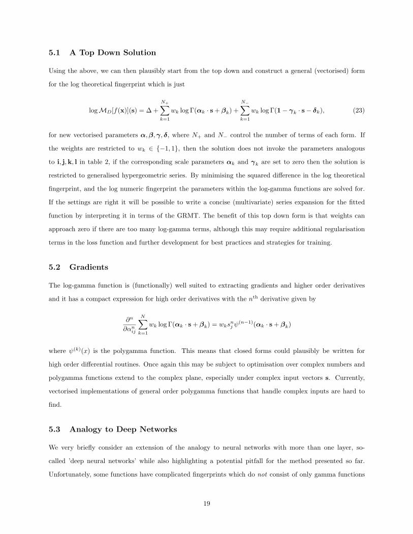
5.1 A Top Down Solution

Using the above, we can then plausibly start from the top down and construct a general (vectorised) form

for the log theoretical fingerprint which is just

logMD[f(x)](s) = ∆+

N+∑

k=1

wk log Γ(αk · s+ βk) +

N−∑

k=1

wk log Γ(1− γk · s− δk), (23)

for new vectorised parameters α,β,γ, δ, where N+ and N− control the number of terms of each form. If

the weights are restricted to wk ∈ {−1, 1}, then the solution does not invoke the parameters analogous

to i, j,k, l in table 2, if the corresponding scale parameters αk and γk are set to zero then the solution is

restricted to generalised hypergeometric series. By minimising the squared difference in the log theoretical

fingerprint, and the log numeric fingerprint the parameters within the log-gamma functions are solved for.

If the settings are right it will be possible to write a concise (multivariate) series expansion for the fitted

function by interpreting it in terms of the GRMT. The benefit of this top down form is that weights can

approach zero if there are too many log-gamma terms, although this may require additional regularisation

terms in the loss function and further development for best practices and strategies for training.

5.2 Gradients

The log-gamma function is (functionally) well suited to extracting gradients and higher order derivatives

and it has a compact expression for high order derivatives with the nth derivative given by

∂n

∂αnij

N∑

k=1

wk log Γ(αk · s+ βk) = wksnj ψ

(n−1)(αk · s+ βk)

where ψ(k)(x) is the polygamma function. This means that closed forms could plausibly be written for

high order differential routines. Once again this may be subject to optimisation over complex numbers and

polygamma functions extend to the complex plane, especially under complex input vectors s. Currently,

vectorised implementations of general order polygamma functions that handle complex inputs are hard to

find.

5.3 Analogy to Deep Networks

We very briefly consider an extension of the analogy to neural networks with more than one layer, so-

called ’deep neural networks’ while also highlighting a potential pitfall for the method presented so far.

Unfortunately, some functions have complicated fingerprints which do not consist of only gamma functions

19

and their reciprocals. Take for example the surprisingly simple function f(x1) = e−x21/3−x1 , whose Mellin

transform is given by

M[f(x1)](s1) =3s1/2Γ(s1)

2s1U

(s1

2,1

2,3

4

)

(24)

where U(a, b, x) is the Tricomi hypergeometric function. The nice property of the Mellin transform is that

this hypergeometric function is still related to gamma functions. If we include a ‘virtual’ parameter x2, such

that when x2 = 1 the previous expression is preserved, we could perform a second Mellin transform such as

Mx2→s2 [Mx1→s1 [f(x1)]](s1, s2) = Mx2→s2

[3s1/2Γ(s1)

2s1U

(s1

2,1

2,3x24

)]

= 3(s1−2s2)/2Γ(s1

2− s2

)

Γ(2s2),

(25)

where we now see the right-hand side is comprised of gamma functions, and powers of constants in a way

that is representable as a two-dimensional Mellin transform

M2[f(x1, x2)]](s) = 3a·sΞ [As] , a =

[1

2,−1

]

, A =

12 −1

0 2

(26)

Using the above iterated process we can construct an analogy to a deeper neural network, where each (hid-

den) layer requires another Mellin transform with respect to a virtual parameter. If this could be generalised

and implemented seamlessly, the algorithm would be able to detect a much wider range of functions and dis-

tributions. However, for data driven problems the analogy cannot be realised, because each Mellin transform

was equivalent to a sampling operation from some distribution, and the new intermediate virtual distribution

is not well defined from the input numeric data.

In this vein, Rathie et al. have devloped a Y-function, where the gamma functions are replaced by Tricomi

hypergeometric functions [20]. The significance of this is that these hypergeometric functions themselves can

be expressed through an inverse Mellin transform. These advanced functions may be closer in analogy to

an iterated, or second layer, requiring a Mellin Transform of the fingerprint, to give the fingerprint of the

fingerprint. Rathie goes on to define functions which replace the gamma functions with other generalised

functions including incomplete gamma functions and Fox-H functions. We leave the development of this

idea for future work, but if these further representations could be harnessed, many more functions could be

recognised. It may be possible to fit not only log-gamma functions, but also log-hypergeometric functions

to the moments. The downside of this is that high order hypergeometric functions are harder to fit due to

varying domains of convergence and analytic continuation and they can be numerically expensive to evaluate.

20

6 Conclusions

We have presented a framework for representing and working with unknown functions with an aim to ap-

plying machine learning techniques and tools to mathematically classify unknown distributions. We call this

process exact learning, because if the resulting parameters of the fitting process are understood in the right

context it may be possible to reconstruct a formula for the unknown distribution. We developed a few ideas

within this framework including the notion of a ‘fingerprint’ of a function in a transformed space which is

easier to traverse when attempting to identify the function. We used the Mellin transform and its inverse as

a tool to switch between the representation spaces, and we noted an extensive hierarchy of functions exists in

the literature whose fingerprints are comprised of gamma functions, with shift, scale and power parameters

along with constants and scaled constant terms. We believe these functions to be a promising starting point

to build exact learning algorithms, interpret the outcomes in a human readable way and categorise and

document unknown numeric solutions. We have shown that multivariate analogues exist for these functions

and methods, and indicated that the exact learning method may scale to high dimensional numeric data and

requires relatively few parameters to learn the fingerprint.

We found that a multivariate extension of the most generalised function can take a relatively compact

form, and the log of the theoretical fingerprint begins to resemble an unsupervised network. A natural anal-

ogy exists between a single layer neural network with a ‘log-gamma’ activation function or basis function.

There are also possible extensions to deeper networks with more layers and this new perspective may be a

step towards explaining how neural networks work and interpreting the coefficients and weights in the same

way that the hierarchy of functions is developed. The log-gamma activation function has particularly nice

derivatives, but a complex branch structure will undoubtedly require new techniques for efficient training

and optimisation.

Further developments could include the addition of polygamma terms as well as gamma terms to the fin-

gerprint which would relate to series expansions containing powers of logarithms as well as monomial terms.

One could also imagine a larger network which is comprised of multiple exact learning ‘units’ containing sums

of terms, products of terms and compositions of functions. Sums of functions would be trivial to implement,

but further mathematical developments would be required train such networks for products including Mellin

convolution and development of the equivalent of a Ramanujan master theorem for arbitrary trees of binary

operations on functions.

21

The supplementary materials contain extended discussion on future work and the limitations of the

methods we presented here. We also implemented some basic versions of the exact learning algorithm along

with a basic method for fitting the fingerprints using complex numbers. The key limitations of the method

presented here is that functions are currently restricted to the domain [0,∞)n, and must be representable

by the hierarchy of functions described by a Mellin-Barnes integral, which as we showed does not cover even

some simple examples of functions. The method used for sampling moments for these prototypes is crude,

and the results are currently demonstrable for bound ‘distribution’ like functions for which the whole domain

has been sampled. With numeric Mellin transforms, and advanced sampling and training methods we hope

to see ‘exact learning’ evolve into a more sophisticated method which makes useful discoveries in many fields

of science. We believe the representation presented here is a good starting point for further developments.

7 Acknowledgements

B. W. J. Irwin acknowledges the majority of the research was made during his time in the EPSRC Centre

for Doctoral Training in Computational Methods for Materials Science for funding under grant number

EP/L015552/1.

References

[1] Diogo V. Carvalho, Eduardo M. Pereira, and Jaime S. Cardoso. Machine learning interpretability: A

survey on methods and metrics. Electronics (Switzerland), 8(8):1–34, 2019.

[2] Yann Lecun, Yoshua Bengio, and Geoffrey Hinton. Deep learning. 2015.

[3] Eve Belisle, Zi Huang, Sebastien Le Digabel, and Aımen E Gheribi. Evaluation of machine learning

interpolation techniques for prediction of physical properties. Computational Materials Science, 98:170–

177, 2015.

[4] Simon Plouffe. Inverse Symbolic Calculator, 1986.

[5] Robert Munafo. RIES, 1996.

[6] Ivan Gonzalez, Victor H. Moll, and Ivan Schmidt. Ramanujan’s Master Theorem applied to the evalu-

ation of Feynman diagrams. Advances in Applied Mathematics, 63:214–230, 2015.

[7] Lorenzo Rosasco, Ernesto De Vito, Andrea Caponnetto, Michele Piana, and Alessandro Verri. Are Loss

Functions All the Same? Neural Computation, 16(5):1063–1076, may 2004.

22

[8] Sebastian Ruder. An overview of gradient descent optimization algorithms. pages 1–14, sep 2016.

[9] Haohan Wang and Bhiksha Raj. On the Origin of Deep Learning. pages 1–72, feb 2017.

[10] Martın Abadi, Paul Barham, Jianmin Chen, Zhifeng Chen, Andy Davis, Jeffrey Dean, Matthieu Devin,

Sanjay Ghemawat, Geoffrey Irving, Michael Isard, Manjunath Kudlur, Josh Levenberg, Rajat Monga,

Sherry Moore, Derek G Murray, Benoit Steiner, Paul Tucker, Vijay Vasudevan, Pete Warden, Martin

Wicke, Yuan Yu, Xiaoqiang Zheng, Google Brain, Implementation Osdi, Paul Barham, Jianmin Chen,

Zhifeng Chen, Andy Davis, Jeffrey Dean, Matthieu Devin, Sanjay Ghemawat, Geoffrey Irving, Michael

Isard, Manjunath Kudlur, Josh Levenberg, Rajat Monga, Sherry Moore, Derek G Murray, Benoit

Steiner, Paul Tucker, Vijay Vasudevan, Pete Warden, Martin Wicke, Yuan Yu, and Xiaoqiang Zheng.

TensorFlow : A System for Large-Scale Machine Learning This paper is included in the Proceedings of

the TensorFlow : A system for large-scale machine learning. 2016.

[11] Adam Paszke, Sam Gross, Francisco Massa, Adam Lerer, James Bradbury, Gregory Chanan, Trevor

Killeen, Zeming Lin, Natalia Gimelshein, Luca Antiga, Alban Desmaison, Andreas Kopf, Edward Yang,

Zachary DeVito, Martin Raison, Alykhan Tejani, Sasank Chilamkurthy, Benoit Steiner, Lu Fang, Junjie

Bai, and Soumith Chintala. PyTorch: An Imperative Style, High-Performance Deep Learning Library.

In H Wallach, H Larochelle, A Beygelzimer, F d\textquotesingle Alche-Buc, E Fox, and R Garnett,

editors, Advances in Neural Information Processing Systems 32, pages 8024–8035. Curran Associates,

Inc., 2019.

[12] Daniel Greenfeld and Uri Shalit. Robust Learning with the Hilbert-Schmidt Independence Criterion.

(1):1–25, oct 2019.

[13] George Fikioris. Integral evaluation using the mellin transform and generalized hypergeometric func-

tions: Tutorial and applications to antenna problems. IEEE Transactions on Antennas and Propagation,

54(12):3895–3907, 2006.

[14] K. S. Kolbig, I. S. Gradshteyn, I. M. Ryzhik, Alan Jeffrey, and Inc. Scripta Technica. Table of Integrals,

Series, and Products., volume 64. 1995.

[15] Arjun K Rathie. A New Generalization of Generalized Hypergeometric Functions. Le Matematiche,

52(2):297–310, 1997.

[16] E Maitland Wright. The Asymptotic Expansion of the Generalized Hypergeometric Function. Journal

of the London Mathematical Society, s1-10(4):286–293, oct 1935.

23

[17] Charles Fox. The G and H Functions as Symmetrical Fourier Kernels. Transactions of the American

Mathematical Society, 98(3):395, 1961.

[18] A. A. Inayat-Hussain. New properties of hypergeometric series derivable from Feynman integrals II. A

generalisation of the H function. Journal of Physics A: General Physics, 20(13):4119–4128, 1987.

[19] Francesco Mainardi and Gianni Pagnini. Salvatore Pincherle: The pioneer of the Mellin-Barnes integrals.

Journal of Computational and Applied Mathematics, 153(1-2):331–342, 2003.

[20] Pushpa N. Rathie, Arjun K. Rathie, and Luan C. de S. M. Ozelim. On the Distribution of the Product

and the Sum of Generalized Shifted Gamma Random Variables. pages 1–9, 2013.

[21] Arjun Kumar Rathie, Luan Carlos de Sena Monteiro Ozelim, and Pushpa Narayan Rathie. On a new

identity for the H-function with applications to the summation of hypergeometric series. Turkish Journal

of Mathematics, 42(3):924–935, 2018.

[22] Charlotte Sleight. A Mellin space approach to cosmological correlators. Journal of High Energy Physics,

2020(1), 2020.

[23] M. Passare, A. K. Tsikh, and A. A. Cheshel. Multiple Mellin-Barnes integrals as periods of Calabi-Yau

manifolds with several moduli. Theoretical and Mathematical Physics, 109(3):1544–1555, 1996.

[24] Ray Daniel Sameshima. On Different Parametrizations of Feynman Integrals. PhD thesis, 2019.

[25] A. Liam Fitzpatrick, Jared Kaplan, Joao Penedones, Suvrat Raju, and Balt C. Van Rees. A natural

language for AdS/CFT correlators. Journal of High Energy Physics, 2011(11), 2011.

[26] J. Twamley and G. J. Milburn. The quantum Mellin transform. New Journal of Physics, 8, 2006.

[27] S. C. Woon. Analytic Continuation of Bernoulli Numbers, a New Formula for the Riemann Zeta

Function, and the Phenonmenon of Scattering of Zeros. 70(1), 1997.

[28] Lance A Waller, Bruce W Turnbull, and J Michael Hardin. Obtaining Distribution Functions by Numer-

ical Inversion of Characteristic Functions with Applications. The American Statistician, 49(4):346–350,

apr 1995.

[29] Silvia Spataru, Taru Academy, and Economic Studies. Applying the Moment Generating Functions to

the Study of Probability Distributions. Informatica Economica Journal, 11(2):132–137, 2007.

[30] A. Erdelyi and H. Bateman. Tables of Integral Transforms I. 1953.

24

[31] Peter Zsohar. Short introduction to the generalized method of moments. Hungarian Statistical Review,

Special(16):150–170, 2012.

[32] Grace Wahba. An introduction to reproducing kernel hilbert spaces and why they are so useful. IFAC

Proceedings Volumes, 36(16):525–528, 2003.

[33] Dinesh S Thakur. Gamma Functions for Function Fields and Drinfeld Modules. Annals of Mathematics,

134(1):25–64, 1991.

[34] T. M. MacRobert. Barnes Integrals as a Sum of E-Functions. Math Annalen., 1962.

[35] Gery Geenens. Mellin-Meijer-kernel density estimation on R+. jul 2017.

[36] Richard Jason Peasgood. A Method to Symbolically Compute Convolution Integrals by. PhD thesis,

2009.

[37] Diederik P. Kingma and Jimmy Lei Ba. Adam: A method for stochastic optimization. 3rd International

Conference on Learning Representations, ICLR 2015 - Conference Track Proceedings, pages 1–15, 2015.

[38] Tewodros Amdeberhan, Olivier Espinosa, Ivan Gonzalez, Marshall Harrison, Victor H Moll, and Armin

Straub. Ramanujan’s Master Theorem. The Ramanujan Journal, 29(1-3):103–120, dec 2012.

[39] Christian Kleiber and Jordan Stoyanov. Multivariate distributions and the moment problem. Journal

of Multivariate Analysis, 113:7–18, jan 2013.

[40] I A Antipova. Inversion of multidimensional Mellin transforms. Russian Mathematical Surveys,

62(5):977–979, 2007.

[41] Kasper J. Larsen and Robbert Rietkerk. MULTIVARIATERESIDUES: A Mathematica package for

computing multivariate residues. Computer Physics Communications, 222:250–262, 2018.

[42] Ivan Gonzalez and Victor H. Moll. Definite integrals by the method of brackets. Part 1. Advances in

Applied Mathematics, 45(1):50–73, 2010.

[43] Ivan Gonzalez, Victor H. Moll, and Ivan Schmidt. Ramanujan’s Master Theorem applied to the evalu-

ation of Feynman diagrams. Advances in Applied Mathematics, 63:214–230, 2015.

[44] Ivan Gonzalez, Karen T Kohl, and Victor H Moll. Evaluation of entries in Gradshteyn and Ryzhik

employing the method of brackets. Number January 2014, pages 195–214. oct 2015.

[45] Vladimir V. Bytev and Bernd A. Kniehl. Derivatives of any Horn-type hypergeometric functions with

respect to their parameters. Nuclear Physics B, 952:114911, 2020.

25

[46] B. C. Carlson. Lauricella’s hypergeometric function FD. Journal of Mathematical Analysis and Appli-

cations, 7(3):452–470, 1963.

[47] J Kampe de Feriet. La fonction hypergeometrique. 85 p. Mem. Sci. math. 85 (1937)., 1937.

26

Figures

Figure 1

An example of the exact learning process, in this case with an example of the kernel of themassless Feynman bubble calculation given by Gonzalez et al. [6]. (Top left), A high precision numericalfunction is found as the solution to a problem that likely has an analytic solution, but the closed form ishard to derive mathematically. A numeric Mellin transform is made from the functiondoma ′ (yellow)∫othe�ngerprint domain' (blue) for a number of chosen exponent vectors s =

(s1; ... ; s2). A highly generalised closed form for the �ngerprint is chosen and then machine learning(function �tting) is used to track down the parameters of the function �ngerprint (a; b; c; d). With furtheranalysis and interpretation of the solved parameters the �ngerprint could be used to derive the closedform for the function that generated the original numeric data using the generalised Ramanujan mastertheorem (GMRT). 

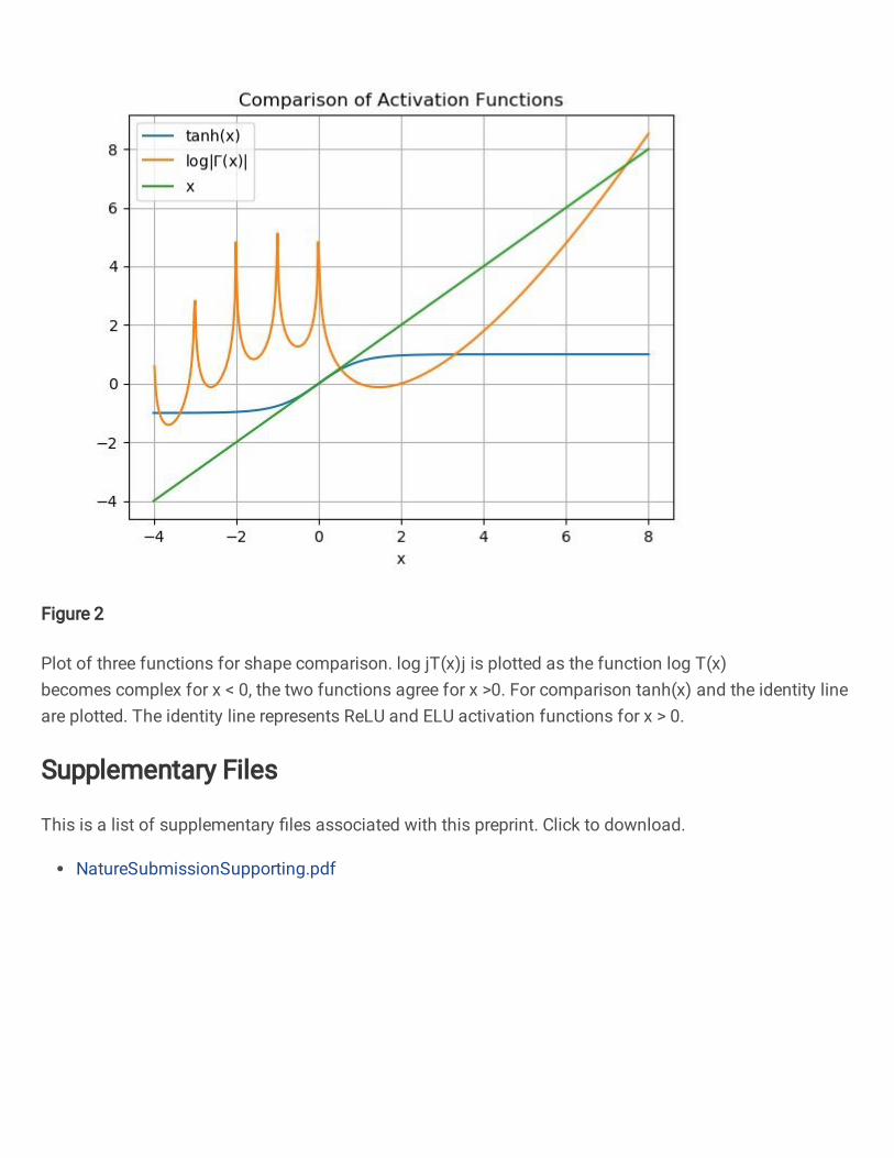
Figure 2

Plot of three functions for shape comparison. log jT(x)j is plotted as the function log T(x)becomes complex for x < 0, the two functions agree for x >0. For comparison tanh(x) and the identity lineare plotted. The identity line represents ReLU and ELU activation functions for x > 0.

Supplementary Files

This is a list of supplementary �les associated with this preprint. Click to download.

NatureSubmissionSupporting.pdf