a n d A r r a y I n v a r i a n t s D I G : A D y n a m i ...
30
30 DIG: A Dynamic Invariant Generator for Polynomial and Array Invariants THANHVU NGUYEN and DEEPAK KAPUR, University of New Mexico WESTLEY WEIMER, University of Virginia STEPHANIE FORREST, University of New Mexico This article describes and evaluates DIG, a dynamic invariant generator that infers invariants from observed program traces, focusing on numerical and array variables. For numerical invariants, DIG supports both nonlinear equalities and inequalities of arbitrary degree defined over numerical program variables. For array invariants, DIG generates nested relations among multidimensional array variables. These properties are nontrivial and challenging for current static and dynamic invariant analysis methods. The key difference between DIG and existing dynamic methods is its generative technique, which infers invariants directly from traces, instead of using traces to filter out predefined templates. To generate accurate invariants, DIG employs ideas and tools from the mathematical and formal methods domains, including equation solving, polyhedra construction, and theorem proving; for example, DIG represents and reasons about polynomial invariants using geometric shapes. Experimental results on 27 mathematical algorithms and an implemen- tation of AES encryption provide evidence that DIG is effective at generating invariants for these programs. Categories and Subject Descriptors: D.2.4 [Software Engineering]: Software/Program Verification—Vali- dation; F.3.1 [Logics and Meanings of Programs]: Specifying, Verifying and Reasoning about Programs— Invariants General Terms: Algorithms, Experimentation, Verification, Theory Additional Key Words and Phrases: Program analysis, dynamic analysis, invariant generation, nonlinear invariants, array invariants, geometric invariant inference, theorem proving ACM Reference Format: Thanhvu Nguyen, Deepak Kapur, Westley Weimer, and Stephanie Forrest. 2014. DIG: A dynamic invariant generator for polynomial and array invariants. ACM Trans. Softw. Eng. Methodol. 23, 4, Article 30 (August 2014), 30 pages. DOI: http://dx.doi.org/10.1145/2556782 1. INTRODUCTION Program invariants are asserted properties, such as relations among variables, at certain locations in a program. By encoding program semantics as logical formulas, in- variants allow for program verification using knowledge from mathematical logic, for example, to prove that a program meets required specifications or is free of certain types of errors. Invariants are also useful in other phases of programming, including docu- mentation, design, coding, testing, debugging, optimization, and maintenance [Ernst 2000]. Thus, the study of invariants is a cornerstone of program analysis [Karr 1976; Jones et al. 1993; Ernst et al. 2007] and has been a major research area since the This work was partially supported by the AFOSR (FA9550-07-1-0532, FA9550-10-1-0277), DARPA (P-1070- 113237), DOE (DE-AC02-05CH11231), NSF (SHF-0905236, CCF-0709097, CNS-0905222) and the Santa Fe Institute. Authors’ addresses: T. Nguyen (corresponding author), D. Kapur, and S. Forrest, Computer Science De- partment, University of New Mexico; W. Weimer, Computer Science Department, University of Virginia; corresponding author’s email: [email protected]. Permission to make digital or hard copies of all or part of this work for personal or classroom use is granted without fee provided that copies are not made or distributed for profit or commercial advantage and that copies bear this notice and the full citation on the first page. Copyrights for components of this work owned by others than ACM must be honored. Abstracting with credit is permitted. To copy otherwise, or republish, to post on servers or to redistribute to lists, requires prior specific permission and/or a fee. Request permissions from [email protected]. c 2014 ACM 1049-331X/2014/08-ART30 $15.00 DOI: http://dx.doi.org/10.1145/2556782 ACM Transactions on Software Engineering and Methodology, Vol. 23, No. 4, Article 30, Pub. date: August 2014.
Transcript of a n d A r r a y I n v a r i a n t s D I G : A D y n a m i ...

30
DIG: A Dynamic Invariant Generator for Polynomialand Array Invariants
THANHVU NGUYEN and DEEPAK KAPUR, University of New MexicoWESTLEY WEIMER, University of VirginiaSTEPHANIE FORREST, University of New Mexico
This article describes and evaluates DIG, a dynamic invariant generator that infers invariants from observedprogram traces, focusing on numerical and array variables. For numerical invariants, DIG supports bothnonlinear equalities and inequalities of arbitrary degree defined over numerical program variables. For arrayinvariants, DIG generates nested relations among multidimensional array variables. These properties arenontrivial and challenging for current static and dynamic invariant analysis methods. The key differencebetween DIG and existing dynamic methods is its generative technique, which infers invariants directlyfrom traces, instead of using traces to filter out predefined templates. To generate accurate invariants, DIGemploys ideas and tools from the mathematical and formal methods domains, including equation solving,polyhedra construction, and theorem proving; for example, DIG represents and reasons about polynomialinvariants using geometric shapes. Experimental results on 27 mathematical algorithms and an implemen-tation of AES encryption provide evidence that DIG is effective at generating invariants for these programs.
Categories and Subject Descriptors: D.2.4 [Software Engineering]: Software/Program Verification—Vali-dation; F.3.1 [Logics and Meanings of Programs]: Specifying, Verifying and Reasoning about Programs—Invariants
General Terms: Algorithms, Experimentation, Verification, Theory
Additional Key Words and Phrases: Program analysis, dynamic analysis, invariant generation, nonlinearinvariants, array invariants, geometric invariant inference, theorem proving
ACM Reference Format:Thanhvu Nguyen, Deepak Kapur, Westley Weimer, and Stephanie Forrest. 2014. DIG: A dynamic invariantgenerator for polynomial and array invariants. ACM Trans. Softw. Eng. Methodol. 23, 4, Article 30 (August2014), 30 pages.DOI: http://dx.doi.org/10.1145/2556782
1. INTRODUCTION
Program invariants are asserted properties, such as relations among variables, atcertain locations in a program. By encoding program semantics as logical formulas, in-variants allow for program verification using knowledge from mathematical logic, forexample, to prove that a program meets required specifications or is free of certain typesof errors. Invariants are also useful in other phases of programming, including docu-mentation, design, coding, testing, debugging, optimization, and maintenance [Ernst2000]. Thus, the study of invariants is a cornerstone of program analysis [Karr 1976;Jones et al. 1993; Ernst et al. 2007] and has been a major research area since the
This work was partially supported by the AFOSR (FA9550-07-1-0532, FA9550-10-1-0277), DARPA (P-1070-113237), DOE (DE-AC02-05CH11231), NSF (SHF-0905236, CCF-0709097, CNS-0905222) and the Santa FeInstitute.Authors’ addresses: T. Nguyen (corresponding author), D. Kapur, and S. Forrest, Computer Science De-partment, University of New Mexico; W. Weimer, Computer Science Department, University of Virginia;corresponding author’s email: [email protected] to make digital or hard copies of all or part of this work for personal or classroom use is grantedwithout fee provided that copies are not made or distributed for profit or commercial advantage and thatcopies bear this notice and the full citation on the first page. Copyrights for components of this work owned byothers than ACM must be honored. Abstracting with credit is permitted. To copy otherwise, or republish, topost on servers or to redistribute to lists, requires prior specific permission and/or a fee. Request permissionsfrom [email protected]©∞ 2014 ACM 1049-331X/2014/08-ART30 $15.00
DOI: http://dx.doi.org/10.1145/2556782
ACM Transactions on Software Engineering and Methodology, Vol. 23, No. 4, Article 30, Pub. date: August 2014.
30:2 T. Nguyen et al.
1970s [Wegbreit 1974; German and Wegbreit 1975; Katz and Manna 1976; Karr 1976;Suzuki and Ishihata 1977; Dershowitz and Manna 1978].
Invariants can be identified from programs using static or dynamic analysis. Staticanalysis discovers invariants by inspecting program code directly, and thus often hasthe advantage of providing sound results that are valid for any program input. Therequirement that invariants be sound leads to expensive computations arising fromthe difficulty of analyzing complex program structures. In contrast, dynamic analysisinfers invariants from traces gathered from program executions over a sample of testcases. The accuracy of the inferred invariant thus depends on the quality and complete-ness of the test cases. However, dynamic analysis is generally efficient and scales wellto complex programs because it focuses on traces, rather than program structures. Forthese reasons, dynamic methods have received considerable attention in practice. Re-cently, for example, dynamically inferred invariants have been used to prevent securityattacks in Mozilla Firefox [Perkins et al. 2009].
A dynamic invariant detector is typically initialized with a predefined collection of in-variant templates postulated to be useful and likely to occur in programs. The detectorfilters out invalid templates based on observed program traces and returns the remain-ders as candidate invariants. Such an approach of checking and filtering is efficient,but it cannot find invariants that are inexpressible under the predefined templates.This article is concerned with two such examples: relations over general polynomialsof numerical and array variables. Polynomials are fundamental to many scientific andengineering applications. Nonlinear polynomials, for example, are especially usefulfor the analysis of hybrid systems [Roozbehani et al. 2005; Sankaranarayanan et al.2005]. ASTREE [Cousot et al. 2005a; Blanchet et al. 2003], a successful static analyzerused to verify the absence of runtime errors in Airbus avionic systems, implements astatic analysis involving the ellipsoid abstract domain to represent and reason abouta class of quadratic inequality invariants.1 Arrays are a widely used data structurethat is essential to the success of many programs. Fixed-size arrays are also present inmany systems programs, and proper reasoning is often critical for security (e.g., bufferoverruns) and performance (e.g., for bounds check elimination [Bodık et al. 2000]). Themajor impediment for finding these invariants dynamically is the prohibitively largenumber of possible templates, for example, each relation involving polynomials of dif-ferent degrees or different numbers of variables would require a separate template.For example, Daikon [Ernst 2000; Ernst et al. 2007], the pioneer of dynamic invariantanalysis, detects only linear relations over at most three variables and has limitedsupport for array relations.
This article describes and evaluates DIG, a dynamic invariant generator that findspolynomial and array relations over program execution traces. DIG uses parameterizedtemplates and computes the unknown coefficients in the templates directly from traces.Consequently, the resulting invariants represented by the instantiated templates areprecise over the input traces. DIG also creates terms to represent information aboutvariables such as nonlinear polynomials over numerical variables. These techniquesallow us to discover invariants that are more expressive than those considered bycurrent dynamic methods.
DIG takes as input a set of traces consisting of values from numerical (reals andintegers) or array variables captured at any program points, including entrance/exitpoints of functions or heads of loops. Depending on the invariants of interest, differenttechniques are used to generate invariants over the input traces. We view polynomial
1The ellipsoid domain for this case is expressed by the quadratic form x2 + axy + y2 ¸≥ k, where 0 < b < 1and a2 < 4b [Feret 2004].
ACM Transactions on Software Engineering and Methodology, Vol. 23, No. 4, Article 30, Pub. date: August 2014.
DIG: A Dynamic Invariant Generator for Polynomial and Array Invariants 30:3
equations and inequalities over variables as geometric shapes in multidimensionalspace: trace data as points, equations as hyperplanes, and conjunctions of inequalitiesas convex polyhedra. Thus, we can exploit well-known concepts and efficient algorithmsfrom algebra and geometry to compute these properties accurately.
DIG also generates flat (non-nested) and nested array relations among multidimen-sional array variables (and functions that can be viewed as arrays). To find linearequations among flat arrays, we first find equalities among array elements and thenidentify the relations among array indices from the obtained equalities. We also findnested array relations by performing reachability analysis. Real-world programs oftenuse large arrays, thus we employ automatic theorem proving technologies to reasonabout large arrays more efficiently.
The main contributions of this article are as follows.
—DIG, a dynamic invariant generator that automatically discovers polynomial andarray invariants from program execution traces. We integrate concepts and toolsfrom mathematical fields such as linear algebra, geometry, and formal methods toimprove dynamic analysis. This is the first work to demonstrate the use of dynamicanalysis to generate nontrivial program invariants such as nonlinear polynomial andnested array relations.
—A mapping from the task of inferring polynomial invariants to that of generatinggeometric shapes over points created from input traces. DIG represents equality andinequality constraints among multiple variables as hyperplanes and polyhedra. Poly-hedra in high dimensions are expensive to compute, thus we also consider simplergeometric shapes, such as octagons, which are more tractable because they encodeless expressive constraints. When additional inputs from the user are available, wecan also deduce new inequalities from previously obtained equality relations.
—The use of equation solving and automatic theorem proving to dynamically inferrelations among array variables of multiple dimensions and functions of multiplearguments. In particular, we encode the problem of finding nested array relationsas a satisfiability formula that can be efficiently solved by a satisfiability modulotheories (SMT) solver.
—An empirical evaluation of DIG on a set of 27 programs that have documented invari-ants2 involving nonlinear polynomials. We also evaluated DIG on an implementationof AES encryption that contains documented invariants involving array relations.The tool successfully discovers all documented invariants of the considered polyno-mial and array forms.
A preliminary version of some of these points was published in Nguyen et al. [2012].This article extends those results to include the following.
—Geometric Invariant Inference. By interpreting polynomial relations as geometricshapes, we take advantage of proven concepts and existing algorithms in linearalgebra and geometry to reason about these invariants efficiently. Using geometricreasoning, we prove an underapproximation property of polynomial invariants thatis guaranteed in DIG, but not in other template-based analyses.
—New Forms of Invariants. We extend our earlier work to include octagonal inequali-ties, a special form of constraint that is useful in array bound checks. The techniquefor flat array relations has been extended to identify relations over certain subsetsof array elements, that is, a form of conditional invariants. A modified version of
2Documented invariants refer to information found in the program documentations or source-code commentsdescribing the program behaviors.
ACM Transactions on Software Engineering and Methodology, Vol. 23, No. 4, Article 30, Pub. date: August 2014.
30:4 T. Nguyen et al.
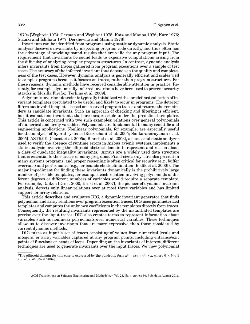
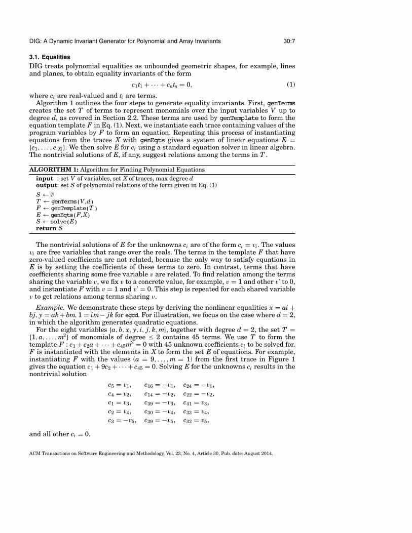
Fig. 1. An extended GCD algorithm and its traces at location L on inputs (a = 9, b = 5) and (a = 182, b =255). From such traces, DIG generates three nonlinear invariants x = ai + bj, y = ak + bm, 1 = im¡− jk.
reachability analysis for generating nested array relations with polynomial runtimecomplexity is also provided.
—Formal Analysis. We describe the time complexity of all presented algorithms. Inparticular, we show that the problem of generating nested array relations belongs tothe polynomial class of complexity by presenting a polynomial-time algorithm for it.
The rest of this article is organized as follow: Section 2 provides a motivating exampleand an overview of DIG. Sections 3 and 4 describe our algorithms for generating poly-nomial and array invariants in detail. Section 5 analyzes the complexity of the givenalgorithms and shows interesting properties of the generated invariants. Section 6reports experimental results. Section 7 surveys related work. Section 8 concludes.
2. MOTIVATING EXAMPLE
We use an example program to highlight the important insights underlying DIG and tomotivate key design decisions. Figure 1 shows an implementation of egcd, an extendedGCD algorithm in number theory that takes as input a pair of integers (a, b) andreturns x = gcd(a, b) and two integers i, j satisfying the Bezout identity x = ai + bj.The main computation of egcd consists of a while loop on lines 4–12, whose semanticsis captured by its loop invariant at location L. The table in Figure 1 consists of severalsets of trace values from the eight variables {a, b, x, y, i, j, k, m} in scope at L for thetwo inputs (a = 9, b = 5) and (a = 182, b = 255).
From such traces, DIG identifies three nonlinear relations x = ai + bj, y = ak + bm,1 = im ¡− jk at location L. The first two are documented invariants for egcd, whichassert the computation and preservation of the Bezout identity in the loop. The thirdrelation is a valid but undocumented invariant, revealing a potentially useful detail:the product im is exactly 1 more than the product jk whenever the program reacheslocation L.
At a high level, DIG treats numerical trace data as points in Euclidean space andcomputes geometric shapes enclosing these points. For example, the trace values ofthe two variables v1, v2 are points in the (v1, v2)-plane. DIG then determines if thesepoints lie on a line, represented by a linear equation of the form c0 + c1v1 + c2v2 = 0.If such a line does not exist, DIG builds a bounded convex polygon from these points.The edges of the polygon are represented by linear inequalities of the form c0 + c1v1 +c2v2 ¸≥ 0. This technique generalizes to equations and inequalities among multiplevariables by constructing hyperplanes and polyhedra in a high-dimensional space. Togenerate nonlinear constraints, DIG uses terms to represent nonlinear polynomialsover program variables, for example, t1 = v1, t2 = v1v2. This allows DIG to generate
ACM Transactions on Software Engineering and Methodology, Vol. 23, No. 4, Article 30, Pub. date: August 2014.

DIG: A Dynamic Invariant Generator for Polynomial and Array Invariants 30:5
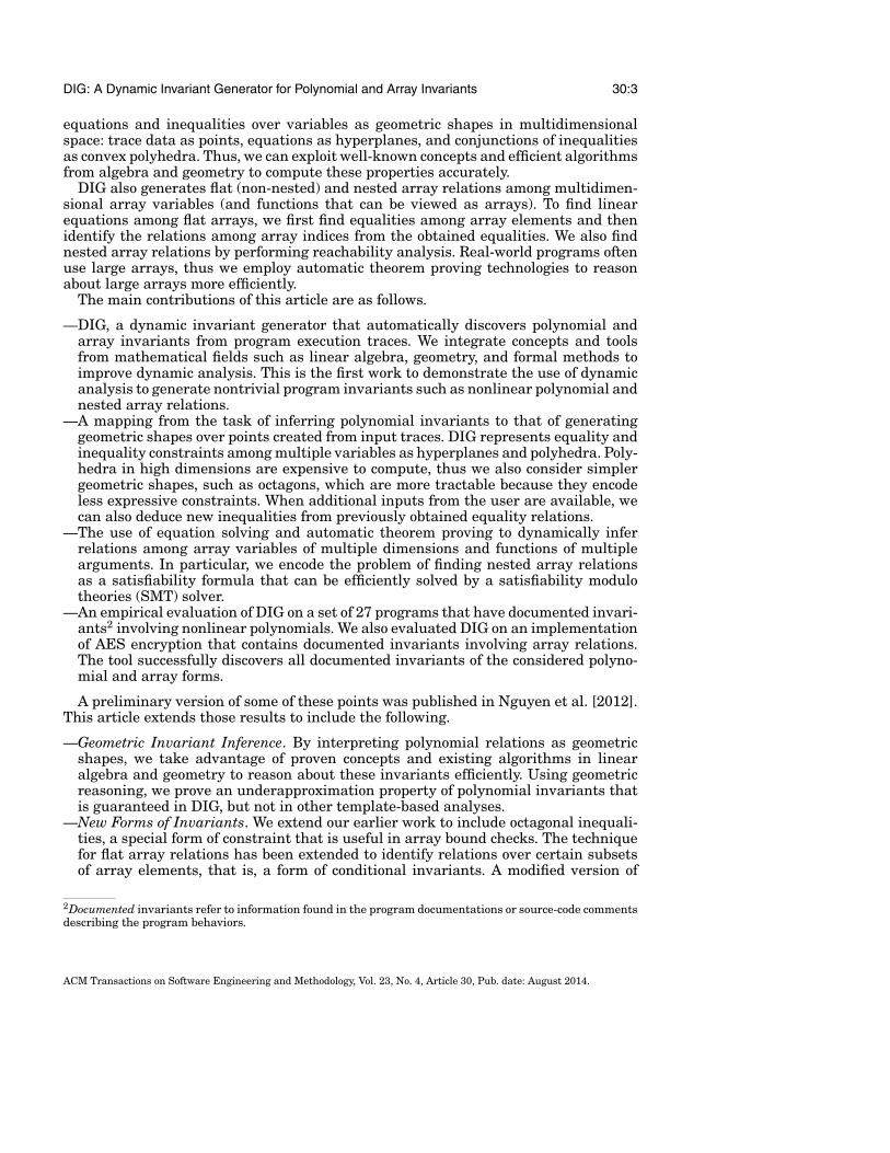
Fig. 2. An overview of DIG. The generator finds different types of invariants from input traces. The post-processing step removes redundant and spurious invariants.
equations such as t1 + t2 = 1, which represents a line over t1, t2 and a hyperbola overv1, v2.
DIG builds geometric shapes in high dimensions that are represented by nonlin-ear constraints over multiple variables or terms. However, constructing such complexshapes from many points is expensive. Thus, DIG also supports constraints repre-senting simpler geometric shapes such as octagons. Octagonal inequalities are lessexpressive than general inequalities, but they are useful for detecting bugs such asarray bounds errors and memory leaks. The modular design of DIG allows for easyextensions to other geometric shapes for other specific forms of invariants.
Returning to the egcd example, terms are generated to represent monomials up toa certain degree over the variables {a, b, x, y, i, j, k, m}. An equation template of theform c1t1 + · · · + cntn = 0 is created from the terms ti. We use the traces in Figure 1to instantiate the template, obtaining a set of equations, which we then solve for theunknowns ci using a standard equation solver. This allows DIG to identify the threeequations x = ia + jb, y = ka + mb, 1 = im¡− jk at location L from the execution tracesof egcd. These nonlinear invariants cannot be discovered by current dynamic analysistools and are also challenging for methods based on static analysis.
We explore these ideas and describe concrete implementation details in the nextsections.
2.1. Overview of DIG
Figure 2 gives an overview of the DIG framework that generates invariants from inputtraces consisting of values from numerical or array variables.3 First, terms are createdto represent variables whose values are captured in the traces. Depending on the typeof the variables from input traces, DIG next generates polynomial relations or arrayrelations over terms. Finally, the post-processing step removes redundant and spuriousinvariants4 and reports the remaining invariants as its output. Optionally, the user canmodify the parameters of DIG for better performance or specify additional informationto aid the invariant generation process, for example, loop conditions as described inSection 3.2.1.
2.2. Terms
We use terms to represent nonlinear properties over program variables and otherinformation of interest. From a set V of variables and a degree d, a set T of terms
3Currently we do not support variables from dynamic data structures that may have values in some execu-tions and may not exist in other executions.4Spurious invariants refer to candidate relations that hold over the observed traces at a program location,but they might not hold over all possible traces at that location.
ACM Transactions on Software Engineering and Methodology, Vol. 23, No. 4, Article 30, Pub. date: August 2014.
30:6 T. Nguyen et al.
is created to represent monomials up to degree d from V. For instance, the set T often terms {1, x, y, i, xy, xi, yi, x2, y2, i2} contains all monomials up to degree 2 over thevariables {x, y, i}. Nonlinear relations over program variables can now be specified aslinear relations over terms, which allows us to generate nonlinear invariants fromexisting techniques for linear constraint solving.
In addition to monomials, the user can manually define terms to capture other desir-able properties, for example, t1 = x
y , t2 = xi, t3 = mod(x, 256). This idea is related to theconcept of derived variables used in Daikon to express additional information [Perkinsand Ernst 2004]. Users can also query DIG for relations among a specific set of terms,for example, only inequalities among {x, y, i2}. These customizations allow DIG toidentify specific relations among potentially interesting terms and reduce the overallcomplexity of the process.
2.3. Post Processing
DIG uses two techniques, pruning and filtering, to help remove redundant and spu-rious invariants. We note that existing strategies from other approaches could alsobe integrated with DIG-generated invariants. For example, if DIG’s algorithms wereincorporated into Daikon, then most of its optimization techniques [Perkins and Ernst2004] could be applied directly to the resulting invariants. Recently, the work re-ported in Sharma et al. [2013] has integrated ideas from DIG to infer sound equalityinvariants.
Pruning. To reduce the number of candidate invariants, DIG removes any invariantsthat are logical implications from other invariants. For instance, we suppress theinvariant x2 = y2 if another invariant x = y is also found, because the latter implies theformer. These redundant invariants arise because we treat each term as an independentvariable for the purpose of finding nonlinear polynomials. For example, if t1 = x, t2 =y, t3 = x2, t4 = y2, then x = y implies x2 = y2; however, their corresponding termrelations, t1 = t2 and t3 = t4, have no direct relation. To verify an implication, we usean SMT solver to show that the negation of that implication is unsatisfiable.
Filtering. DIG uses a subset of the input traces for invariant generation and theremaining traces to check the resulting invariants. Because a program invariant holdsfor any set of traces, it is likely that we can find that same invariant using a smallersubset of the available traces. The candidate invariant, which is obtained using a subsetof traces and might not be true for all observed traces, is then verified against theremaining traces and removed if it fails for any of these traces. This strategy improvesthe runtime of DIG since it is more expensive to generate invariants, especially complexones like 1.2xy ¡− 2.3yz + 3.4zw = 0, than to check that they hold over given traces.
Currently DIG randomly chooses traces for invariant generation and training. Forexample, DIG selects a set of random traces whose size is 1.5 £× the number of terms forinvariant generation and 1,000 random traces for filtering. In future work, we intendto use machine-learning heuristics for more effective partitioning of traces for trainingand learning purposes. We elaborate further the application of filtering for reducingspurious inequality relations in Section 5.2.
3. POLYNOMIAL INVARIANTS
DIG takes as input the set V of variables that are in scope at location L, the associatedtraces X, and a maximum degree d, and returns a set of possible polynomial relationsamong the variables in V whose degree is at most d. The post-processing techniques inSection 2.3 are applied to the obtained relations to suppress redundant relations andto filter out spurious invariants.
ACM Transactions on Software Engineering and Methodology, Vol. 23, No. 4, Article 30, Pub. date: August 2014.
DIG: A Dynamic Invariant Generator for Polynomial and Array Invariants 30:7
3.1. Equalities
DIG treats polynomial equalities as unbounded geometric shapes, for example, linesand planes, to obtain equality invariants of the form
c1t1 + · · · + cntn = 0, (1)
where ci are real-valued and ti are terms.Algorithm 1 outlines the four steps to generate equality invariants. First, genTerms
creates the set T of terms to represent monomials over the input variables V up todegree d, as covered in Section 2.2. These terms are used by genTemplate to form theequation template F in Eq. (1). Next, we instantiate each trace containing values of theprogram variables by F to form an equation. Repeating this process of instantiatingequations from the traces X with genEqts gives a system of linear equations E ={e1, . . . , e|X|}. We then solve E for ci using a standard equation solver in linear algebra.The nontrivial solutions of E, if any, suggest relations among the terms in T .
ALGORITHM 1: Algorithm for Finding Polynomial Equationsinput : set V of variables, set X of traces, max degree doutput: set S of polynomial relations of the form given in Eq. (1)S Ã← ;∅T Ã← genTerms(V ,d)F Ã← genTemplate(T)E Ã← genEqts(F,X)S Ã← solve(E)return S
The nontrivial solutions of E for the unknowns ci are of the form ci = vi. The valuesvi are free variables that range over the reals. The terms in the template F that havezero-valued coefficients are not related, because the only way to satisfy equations inE is by setting the coefficients of these terms to zero. In contrast, terms that havecoefficients sharing some free variable v are related. To find relation among the termssharing the variable v, we fix v to a concrete value, for example, v = 1 and other v0 to 0,and instantiate F with v = 1 and v0 = 0. This step is repeated for each shared variablev to get relations among terms sharing v.
Example. We demonstrate these steps by deriving the nonlinear equalities x = ai +bj, y = ak+ bm, 1 = im¡− jk for egcd. For illustration, we focus on the case where d = 2,in which the algorithm generates quadratic equations.
For the eight variables {a, b, x, y, i, j, k, m}, together with degree d = 2, the set T ={1, a, . . . , m2} of monomials of degree ≤ 2 contains 45 terms. We use T to form thetemplate F : c1 + c2a + · · · + c45m2 = 0 with 45 unknown coefficients ci to be solved for.F is instantiated with the elements in X to form the set E of equations. For example,instantiating F with the values (a = 9, . . . , m = 1) from the first trace in Figure 1gives the equation c1 + 9c2 + · · · + c45 = 0. Solving E for the unknowns ci results in thenontrivial solution
c5 = v1, c16 = ¡−v1, c24 = ¡−v1,c4 = v2, c14 = ¡−v2, c22 = ¡−v2,c1 = v3, c39 = ¡−v3, c41 = v3,c2 = v4, c30 = ¡−v4, c33 = v4,c3 = ¡−v5, c29 = ¡−v5, c32 = v5,
and all other ci = 0.
ACM Transactions on Software Engineering and Methodology, Vol. 23, No. 4, Article 30, Pub. date: August 2014.

30:8 T. Nguyen et al.
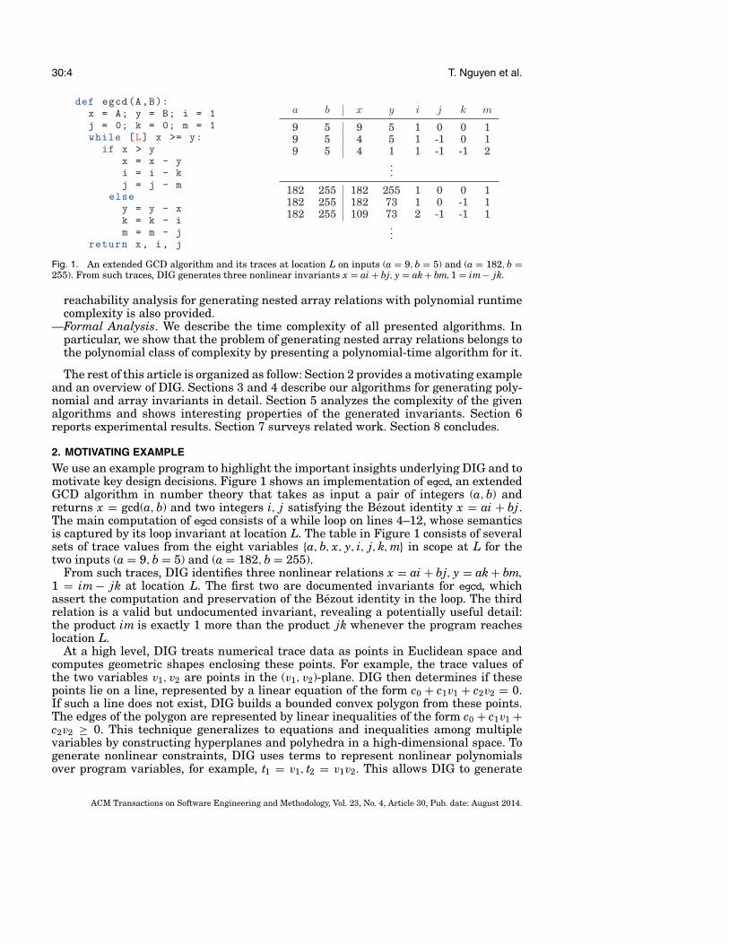
Fig. 3. (a) A set of points in 2D and its approximation using the (b) interval, (c) octagonal, and (d) polyhedralregions.
To find the relation among the terms t5, t16, t24 whose coefficients c5, c16, c24 sharethe value v1, we set v1 = 1 and v2 = v3 = v4 = v5 = 0 (since the terms t5, t16, t24are not related by the values v2,3,4,5). The template F, when being instantiated with(v1 = 1, v2 = v3 = v4 = v5 = 0), gives the relation t5 ¡− t16 ¡− t24 = 0. The terms t5, t16, t24represent the monomials y, bm, ak, thus we obtain the relation y ¡− bm¡− ak = 0.
After repeating this process for all shared variables, the following equations areachieved:
t5 = y, t16 = bm, t24 = ak !→ y = bm+ ak,t4 = x, t14 = ai, t22 = bj !→ x = ai + bj,t1 = 1, t39 = im, t41 = jk !→ 1 = im¡− jk,t2 = a, t30 = mx, t33 = jy !→ a = mx ¡− jy,t3 = b, t29 = kx, t32 = iy !→ b = ¡−kx + iy.
The first three equations are program invariants. The last two relations are redundant,that is, they can be obtained from the first three relations through variable substitu-tions. The post-processing step in Section 2.3 suppresses these redundant invariantsusing theorem proving. The resulting set of equations for egcd after post processing is{y = bm+ ak, x = ai + bj, 1 = im¡− jk}.
3.2. Inequalities
We interpret sets of inequalities among terms as geometric shapes over points createdfrom program traces. Figure 3 depicts several geometrical shapes correspondingto the types of inequalities currently supported in DIG. For illustration purposes,two-dimensional shapes are used to represent linear relations between two terms.Figure 3(a) shows a set of trace points created from input traces. Figures 3(b), 3(c), 3(d)approximate the area enclosing these points using the interval, octagonal, and poly-hedral shapes that are represented by systems of constraints of the forms c1 ≤ v ≤ c2,c1 ≤ ±v1 ± v2 ≤ c2, and c1v1 + · · · + cnvn ≤ 0, respectively. These constraints are sortedby expressive power: polyhedral constraints can express octagonal constraints, whichcan express interval constraints. This order is reversed in complexity: interval shapesare cheaper to compute than octagons, which are cheaper to compute than polyhedra.
3.2.1. General (Polyhedral) Inequalities. DIG finds inequality invariants of the form
c1t1 + · · · + cntn ¸≥ 0, (2)
where ci are real-valued and ti are terms. These general inequalities also representoctagonal inequalities (two terms with specific integral coefficients) and interval in-equalities (single terms with unit coefficients).
Algorithm 2 outlines two techniques for finding general inequalities. The polyhe-dral technique consists of three steps: using terms to represent program variables(genTerms), instantiating points from terms using input traces (genPoints), creating aconvex polyhedron enclosing the points (createPolyhedron), and extracting its facets
ACM Transactions on Software Engineering and Methodology, Vol. 23, No. 4, Article 30, Pub. date: August 2014.

DIG: A Dynamic Invariant Generator for Polynomial and Array Invariants 30:9
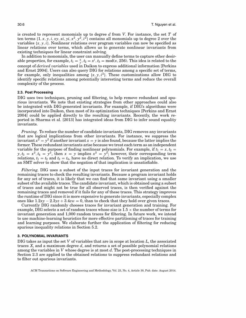
Fig. 4. Cohen’s integer division algorithm and its traces on inputs (x = 15, y = 2) and (x = 4, y = 1).
ALGORITHM 2: Algorithm for Finding Polynomial Inequalitiesinput : set of variables V , set of traces X, max degree dinput : (optional) set of inequalities ieqs from additional information such as loop
conditionsoutput: set S of polynomial inequalitiesS Ã← ;∅if ieqs = ;∅ then
T Ã← genTerms(V ,d)P Ã← genPoints(T ,X)H Ã← createPolyhedron(P)S Ã← extractFacets(H)
endelse
// if additional information is giveneqts Ã← genInvseqts(V ,X,d)S Ã← deduceieqs(eqts,ieqs)
endreturn S
to represent inequalities among terms (extractFacets). When additional informationis available, the alternative technique combines the discovered equations (genInvseqts)with the given information to deduce new inequalities (deduceieqs). Both techniquesgive sound relations with respect to input traces; however the deduction method, withthe help of additional information, runs much faster.
We demonstrate these methods using the cohen program in Figure 4, which has anonlinear inequality invariant and other information that is useful for deduction. cohenimplements the integer division algorithm by Cohen [1990], which takes as input apair of integers (x, y) and returns the integer q as the quotient of x and y. We considerinvariants at location L, the head of the inner while loop. There are six variables{a, b, q, r, x, y} in scope at L. The table in Figure 4 consists of several sets of valuesrepresenting traces obtained from the variables at L for inputs (x = 15, y = 2) and(x = 4, y = 1).
The documented invariants b = ya, x = qy + r, r ¸≥ 2ya describe precisely the seman-tics of the inner while loop in Cohen’s algorithm.5 The first two equations are obtainedusing the technique described in Section 3.1. This section focuses on the third invariant
5The invariant x = qy + r asserts that the dividend x equals the divisor y times the quotient q plus theremainder r.
ACM Transactions on Software Engineering and Methodology, Vol. 23, No. 4, Article 30, Pub. date: August 2014.

30:10 T. Nguyen et al.
that is an inequality of the form given in Eq. (2). For illustration, we again focus on thecase where d = 2, in which the algorithm generates quadratic inequalities.
Using Polyhedra. After the set T of terms is created, the traces X are used to gener-ate points in |T |-dimensional Euclidean space, and the convex hull of these points iscomputed to represent a polyhedron H. The bounded convex polyhedron H can also bedescribed by a system of linear inequalities of the form given in Eq. (2). This is calledthe half-space representation of a polyhedron. The facets of H, corresponding to thesolutions of the system of linear equalities, represent the inequalities among the termsin T . Figure 3(d) depicts a 2D polyhedron (polygon) that has five facets.
The complexity of building H in |T | dimensions is exponential in |T |, as discussedin Section 5.1. The set T generated from the six variables in cohen with degree 2 has28 terms. Building a convex polyhedron in 28 dimensions is not computationallyfeasible, so DIG uses several heuristics to identify possible inequality relations.
We first observe that a program invariant often involves just a small subset ofall possible program variables. For example, the invariant b ¡− ay = 0 involves only{a, b, y} even though all six variables in scope were considered. We experimented withseveral heuristics based on this observation, such as iteratively searching for invariantsinvolving all possible combinations of a small, fixed number of variables. The ability todetermine which variables are important improves performance greatly and is furtherdiscussed in Section 6.3.
Example. DIG first generates possible inequality relations in which at most threeof the six program variables {a, b, q, r, x, y} appear. There are ( 6
3 ) = 20 combinationsthat contain three variables, one of which is {r, y, a}. To find nonlinear inequalities,terms of degree d are built on the variables under consideration. With d = 2, DIGgenerates the set T = {1, r, y, a, ry, ra, ya, r2, y2, a2} of terms.
The elements of T are instantiated with the traces X to form a set P of points. Forinstance, the first trace in Figure 4 gives the point [1, 15, 2, 1, 30, 15, 2, 225, 4, 1] in ten-dimensional Euclidean space corresponding to the terms in T . The convex polyhedronH is then constructed to enclose the points in P. One of the facets of H corresponds tothe documented invariant r ¡−2ya ¸≥ 0. The inequalities represented by other facets arealso valid with respect to the input traces, although they might be spurious invariants.Section 5.2 provides additional discussion on these spurious invariants.
Deduction From Loop Conditions. As previously shown, the polyhedral method forgeneral inequalities does not scale to large numbers of terms. Consequently, we devel-oped an alternative technique using deduction to find inequalities of the form given inEq. (2) if some additional information is available. More specifically, if some inequal-ities are asserted at location L, then DIG can use them together with the discoveredequalities from Section 3.1 to deduce new nontrivial inequalities. For instance, if thelocation L is the head of a loop, then L can be reached if and only if the loop conditionsare met. Such loop conditions are an example of additional information, which canbe given as input from the user (or automatically mined from the source code as inthe cohen program) to facilitate the process of generating additional invariants. Deduc-tion is related to the strategy of adding known facts or proved result as lemmas ininteractive theorem provers such as PVS [Owre et al. 1992].
Example. We demonstrate how deduction is applied to cohen. First, the set of equa-tions {b ¡− ay = 0, qy + r ¡− x = 0} representing possible invariants at location L isobtained, as described in Section 3.1. The head of the inner loop at location L is reachedonly when the condition of that loop r ¸≥ 2b is met, thus r ¡− 2b ¸≥ 0 is also an invariantat L. New and nontrivial inequalities can be deduced from this additional informa-tion using deduction, term rewriting, and substitution. In the current implementation,
ACM Transactions on Software Engineering and Methodology, Vol. 23, No. 4, Article 30, Pub. date: August 2014.
DIG: A Dynamic Invariant Generator for Polynomial and Array Invariants 30:11
we pair inequalities from the loop conditions with the obtained equations to deducenew inequalities. For the running example, r ¡− 2ay ¸≥ 0 is deduced from the pair(r ¡− 2b ¸≥ 0, b¡− ay = 0), and x ¡− qy ¡− 2b ¸≥ 0 is deduced from (r ¡− 2b ¸≥ 0, qy + r ¡− x = 0).Hence, deduction finds the inequalities r ¡−2ya ¸≥ 0, x¡−qy¡−2b ¸≥ 0 among the variables{a, b, q, r, x, y}, both of which are program invariants at location L in cohen.
Deduction could theoretically produce many results by combining discovered equali-ties and loop conditions. However, the technique is efficient in our experiments becausethe number of loop conditions and generated equality invariants is few (one or twoguards at most loops and less than four equalities at a particular program location).Moreover, although we could just use the obtained equalities and loop conditions, theserelations might be opaque to the human user, but the deduced ones are easier to un-derstand (e.g., match the program descriptions). Our experiments in Section 6.2 showsthat deduction allows for effective inequality invariant discovery that otherwise wouldrequire the more expensive polyhedral method or would not be possible in the case ofincomplete traces.
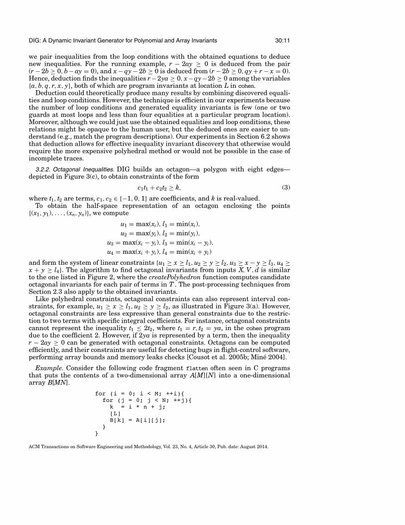
3.2.2. Octagonal Inequalities. DIG builds an octagon—a polygon with eight edges—depicted in Figure 3(c), to obtain constraints of the form
c1t1 + c2t2 ¸≥ k, (3)
where t1, t2 are terms, c1, c2 2∈ {¡−1, 0, 1} are coefficients, and k is real-valued.To obtain the half-space representation of an octagon enclosing the points
{(x1, y1), . . . , (xn, yn)}, we compute
u1 = max(xi), l1 = min(xi),u2 = max(yi), l2 = min(yi),
u3 = max(xi ¡− yi), l3 = min(xi ¡− yi),u4 = max(xi + yi), l4 = min(xi + yi)
and form the system of linear constraints {u1 ¸≥ x ¸≥ l1, u2 ¸≥ y ¸≥ l2, u3 ¸≥ x ¡− y ¸≥ l3, u4 ¸≥x + y ¸≥ l4}. The algorithm to find octagonal invariants from inputs X, V, d is similarto the one listed in Figure 2, where the createPolyhedron function computes candidateoctagonal invariants for each pair of terms in T . The post-processing techniques fromSection 2.3 also apply to the obtained invariants.
Like polyhedral constraints, octagonal constraints can also represent interval con-straints, for example, u1 ¸≥ x ¸≥ l1, u2 ¸≥ y ¸≥ l2, as illustrated in Figure 3(a). However,octagonal constraints are less expressive than general constraints due to the restric-tion to two terms with specific integral coefficients. For instance, octagonal constraintscannot represent the inequality t1 ≤ 2t2, where t1 = r, t2 = ya, in the cohen programdue to the coefficient 2. However, if 2ya is represented by a term, then the inequalityr ¡− 2ay ¸≥ 0 can be generated with octagonal constraints. Octagons can be computedefficiently, and their constraints are useful for detecting bugs in flight-control software,performing array bounds and memory leaks checks [Cousot et al. 2005b; Mine 2004].
Example. Consider the following code fragment flatten often seen in C programsthat puts the contents of a two-dimensional array A[M][N] into a one-dimensionalarray B[MN].
for (i = 0; i < M; ++i){for (j = 0; j < N; ++j){
k = i * n + j;[L]B[k] = A[i][j];
}}
ACM Transactions on Software Engineering and Methodology, Vol. 23, No. 4, Article 30, Pub. date: August 2014.
30:12 T. Nguyen et al.
The nonlinear relation 0 ≤ k ≤ MN ¡− 1 at location L is essential for the safety offlatten and is identified by DIG using octagonal constraints with terms representingquadratic polynomials over variables. The array relation A[i][ j] = B[iN + j], which as-serts the correctness of flatten, is also generated by DIG using the technique describedin the next section.
4. ARRAY INVARIANTS
DIG takes as input the set V of (possibly multidimensional) array variables that are inscope at location L and the associated traces X, and returns a set of possible relationsamong the elements of arrays in V . Currently, we do not consider nonlinear arrayrelations (e.g., A[i]2 = B[i]2 + C[i]2) and therefore do not use terms to represent arrayvariables. The filtering technique given in Section 2.3 also applies to the obtainedrelations to help deal with spurious invariants.6
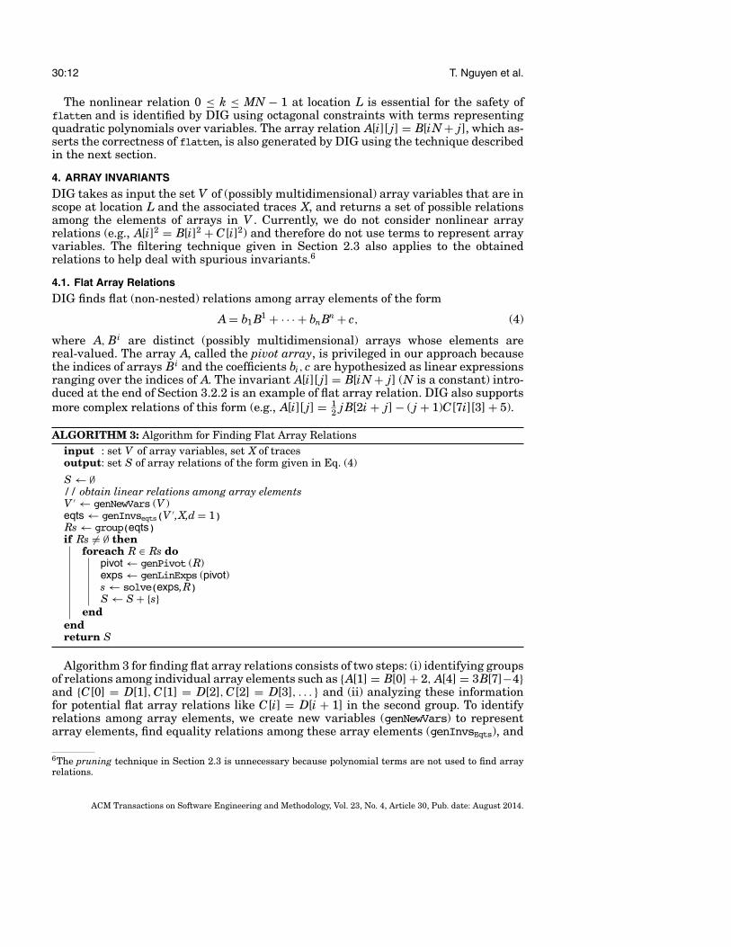
4.1. Flat Array Relations
DIG finds flat (non-nested) relations among array elements of the form
A = b1 B1 + · · · + bnBn + c, (4)
where A, Bi are distinct (possibly multidimensional) arrays whose elements arereal-valued. The array A, called the pivot array, is privileged in our approach becausethe indices of arrays Bi and the coefficients bi, c are hypothesized as linear expressionsranging over the indices of A. The invariant A[i][ j] = B[iN + j] (N is a constant) intro-duced at the end of Section 3.2.2 is an example of flat array relation. DIG also supportsmore complex relations of this form (e.g., A[i][ j] = 1
2 jB[2i + j] ¡− ( j + 1)C[7i][3] + 5).
ALGORITHM 3: Algorithm for Finding Flat Array Relationsinput : set V of array variables, set X of tracesoutput: set S of array relations of the form given in Eq. (4)S Ã← ;∅// obtain linear relations among array elementsV 0 Ã← genNewVars (V )eqts Ã← genInvseqts(V 0,X,d = 1)Rs Ã← group(eqts)if Rs 6= ;∅ then
foreach R 2∈ Rs dopivot Ã← genPivot (R)exps Ã← genLinExps (pivot)s Ã← solve(exps,R)S Ã← S + {s}
endendreturn S
Algorithm 3 for finding flat array relations consists of two steps: (i) identifying groupsof relations among individual array elements such as {A[1] = B[0] + 2, A[4] = 3B[7]¡−4}and {C[0] = D[1], C[1] = D[2], C[2] = D[3], . . . } and (ii) analyzing these informationfor potential flat array relations like C[i] = D[i + 1] in the second group. To identifyrelations among array elements, we create new variables (genNewVars) to representarray elements, find equality relations among these array elements (genInvsEqts), and
6The pruning technique in Section 2.3 is unnecessary because polynomial terms are not used to find arrayrelations.
ACM Transactions on Software Engineering and Methodology, Vol. 23, No. 4, Article 30, Pub. date: August 2014.

DIG: A Dynamic Invariant Generator for Polynomial and Array Invariants 30:13
group the obtained relations (group). To analyze the obtained groups for flat array rela-tions, we represent the relations among the indices of a selected pivot array (genPivot)and other arrays as a parameterized linear expression (genLinExps), instantiate thisexpression with information from the obtained group of equalities, and solve theseequations (solve).
For simplicity, the following explains the algorithm for two one-dimensional arrays,that is, V = {A, B}, although the method generalizes to multidimensional arrays.
Relations among Array Elements. We first generate a set V 0 of new variables repre-senting elements of the arrays in V . Next, the technique from Section 3.1 is used toidentify linear equalities of the form given in Eq. (1) over the variables in V 0 from theinput traces X. The obtained equations represent relations among array elements (e.g.,A4 = 3B7 ¡− 4), where the variables A4, B7, represent the array elements A[4], B[7], re-spectively. Currently, we do not find relations among similar arrays (e.g., A[i] = A[2i]),and thus keep only equations that express relations among array elements of differentarrays. These relations are then grouped so that each group contains relations amongelements from a same set of arrays. For example, {A1 = B0 + 2, A4 = 3B7 ¡− 4} and{C0 = D1, C1 = D2, C2 = D3} are two different groups.
Relations among Array Indices. From each obtained group, we consider only the setR of relations of the form
Ai0 = b0 Bj0 + c0,
Ai1 = b1 Bj1 + c1,
...
where bx, cx are real-valued and Aix , Bjx are the variables in V 0 representing A[ix], B[ jx],respectively.
In such a set R, we select A as the pivot array and hypothesize that the coefficientsbx, cx and the indices jx of array B are linear expressions ranging over the indices ix ofA. For instance, we represent the relation between jx and ix through the parameterizedlinear expression jx = p1ix + q1, where p1 and q1 are unknowns to be solved for. Thisexpression is then instantiated with the information from R to obtain a system ofequations { j0 = p1i0 + q1, j1 = p1i1 + q1, . . . }. Any solution for p and q of theseequations implies a relation of the form A[ix] = (p0ix + q0)B[p1ix + q1] + (p2ix + q2),where ix are the indices of A obtained from R.
The resulting relation ix 2∈ {. . . } )⇒ r has a conditional form where the relation rholds only for specific indices ix of A. Such invariants are useful and appear in manyprograms, for example, in the following codefragment.
for (i=0; i < M; ++i){if (i < 6){
A[i] = [B[4*i], B[4*i+1],B[4*i+2], B[4*i+3]];
}}[L]
For this code fragment, DIG generates the invariant A[i][ j] = B[4i + j] for i ={0, . . . , 5} and j = {0, . . . , 3}, indicating a relation among certain elements of the arraysA and B at location L.
Example. We illustrate the algorithm by finding the relation A[i] = 7B[2i] + 3ibetween two arrays A, B, using traces X that exhibit the relation. An example trace inX contains the values A = [¡−546,¡−641, 34] and B = [¡−78, 3,¡−92,¡−34, 4].
ACM Transactions on Software Engineering and Methodology, Vol. 23, No. 4, Article 30, Pub. date: August 2014.
30:14 T. Nguyen et al.
Eight variables are created to represent the elements of A and B. Based on thegiven trace, the set R = {A0 = 7B0, A1 = 7B2 + 3, A2 = 7B4 + 6} of linear equationsis obtained using the technique in Section 3.1. From R, we choose A as the pivot andextract the information ix = {0, 1, 2}. The relation between jx and ix is expressed asjx = p1ix + q1. We instantiate jx = p1ix + q1 with the information from R and obtainthe set of equations {0 = 0p1 + q1, 2 = 1p1 + q1, 4 = 2p1 + q1}. The unique solution{q1 = 0, p1 = 2} of these equations yields jx = 2ix, that is, A[ix] = bx B[2ix] + cx.Similarly, we instantiate the analogous equations for bx and cx. After solving these, thearray relation ix = {0, 1, 2} )⇒ A[ix] = 7B[2ix] + 3ix is obtained.
Notice that all relations in R have 7 as the coefficient of Bi, thus we can dividethese equations by 7 to obtain R0 = {B0 = 1
7 A0, B2 = 17 A1 ¡− 3
7 , B4 = 17 A2 ¡− 6
7 }. FromR0, we select B as the pivot array and extract the information ix = {0, 2, 4}. Applyingthe preceding process of creating and solving linear equations gives the relation ix ={0, 2, 4} )⇒ B[ix] = 1
7 A[ 12 ix] ¡− 3
14 ix. DIG can recognize such a scenario and thus is ableto generate both array relations.
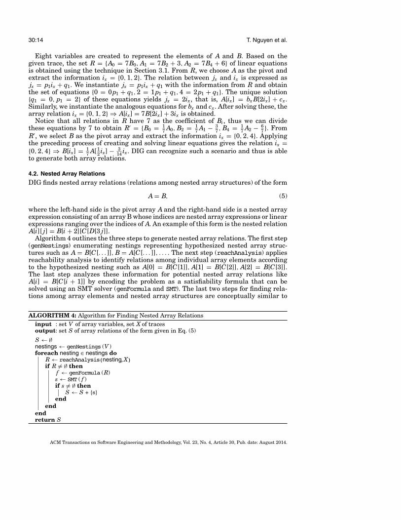
4.2. Nested Array Relations
DIG finds nested array relations (relations among nested array structures) of the form
A = B, (5)
where the left-hand side is the pivot array A and the right-hand side is a nested arrayexpression consisting of an array B whose indices are nested array expressions or linearexpressions ranging over the indices of A. An example of this form is the nested relationA[i][ j] = B[i + 2][C[D[3 j]].
Algorithm 4 outlines the three steps to generate nested array relations. The first step(genNestings) enumerating nestings representing hypothesized nested array struc-tures such as A = B[C[. . . ]], B = A[C[. . . ]], . . . . The next step (reachAnalysis) appliesreachability analysis to identify relations among individual array elements accordingto the hypothesized nesting such as A[0] = B[C[1]], A[1] = B[C[2]], A[2] = B[C[3]].The last step analyzes these information for potential nested array relations likeA[i] = B[C[i + 1]] by encoding the problem as a satisfiability formula that can besolved using an SMT solver (genFormula and SMT). The last two steps for finding rela-tions among array elements and nested array structures are conceptually similar to
ALGORITHM 4: Algorithm for Finding Nested Array Relationsinput : set V of array variables, set X of tracesoutput: set S of array relations of the form given in Eq. (5)S Ã← ;∅nestings Ã← genNestings (V )foreach nesting 2∈ nestings do
R Ã← reachAnalysis(nesting,X)if R 6= ;∅ then
f Ã← genFormula (R)s Ã← SMT ( f )if s 6= ;∅ then
S Ã← S + {s}end
endendreturn S
ACM Transactions on Software Engineering and Methodology, Vol. 23, No. 4, Article 30, Pub. date: August 2014.
DIG: A Dynamic Invariant Generator for Polynomial and Array Invariants 30:15
those of Section 4.1 for flat array relations, but relies on reachability analysis and SMTsolving instead of equation solving.
For simplicity, we illustrate these steps next using three one-dimensional arrays,that is, V = {A, B, C}, although the algorithm generalizes to multidimensional arrays.
Nestings. We first enumerate nested structures among the arrays in V . A nestedarray structure, or nesting, from a set V of arrays is a tuple (P, S), where P is an arrayin V designated as the pivot and S is a nonempty and nonrepeating7 sequence of arraysin V that does not contain the array P. For the input V = {A, B, C}, we generate thenestings (A, [B]), (A, [C]), . . . , (C, [B, A]).
Reachability Analysis. A nesting (A, [B, C]) implies the relation A[i] = B[C[k]], whereelements of the pivot array Aare related to elements of Busing elements of C as indicesinto B. For such a relation to hold, the elements of Amust be in B. Moreover, the indicesof B, where the elements of A appear in, must also be in C. Reachability analysis is ourmethod to determine how the elements of A are related to the elements of B using Cas indices into B.
The analysis could start by checking if all elements of Aare in B. However, this naıveapproach has an exponential complexity when the elements of A occur multiple timesin B. Instead, reachability analysis can be done in polynomial time (Section 5.1) asfollows.
We arbitrarily choose two distinct elements A[x] 6= A[y] from the pivot array A (thereason for using two elements will be justified). For A[x], we find the indices jx in B,where B[ jx] = A[x]. For each of the obtained indices jx in B, we again find the indices kxin C, where C[kx] = jx. We then form a set of relations of the form A[x] = B[C[kx]] fromthese results, which indicate that the element A[x] is related to elements of B usingelements C[kx] as indices into B. Repeating this process for A[y], we obtain a set ofrelations of the form A[y] = B[C[ky]]. Each set R from the cross product of the two setsof relations consists of two equations of the form {A[x] = B[C[kx]], A[y] = B[C[ky]]}.
Note that the relation A[i] = B[C[k]] is determined invalid if any of the precedingchecks fails (e.g., A[x] is not in B or the obtained indices jx of B are in C). We canfurther optimize this algorithm by starting with two distinct elements of A that occurleast often in B. However, such a greedy approach does not guarantee the smallestnumber of relation sets generated at the end because the indices jx of B can occurmany times in C.
Relations among Array Indices. From a set R = {A[x] = B[C[kx], A[y] = B[C[ky]]} ofrelations obtained from reachability analysis, we determine the relation between theindices of A and C. This step is conceptually similar to that of Section 4.1 in whichthe relation between the indices i, k of arrays A, C is represented by the parameterizedlinear expression k = ip + q.
Instantiating k = pi + q with the information from R, we get a system of twoequations {kx = xq + q, ky = yp + q}. The solution for p, q of these equations gives arelation of the form A[i] = B[C[pi + q]], for i = {x, y}. We now verify that this relationalso holds for other indices i of A (instead of just x, y). If it is verified, we return it asthe candidate invariant. Otherwise, we repeat this step on another set R of relationsto find a different nested array relation.
A relation of the form A[i] = B[C[k]] that holds for all indices i of A must also holdfor the two indices (x, y). Thus, we can find such a relation, if it exists, by trying allpossible sets R of relations generated by reachability analysis on the two elements
7The nonrepeating constraint is used to enforce finite depth in the sequence.
ACM Transactions on Software Engineering and Methodology, Vol. 23, No. 4, Article 30, Pub. date: August 2014.
30:16 T. Nguyen et al.
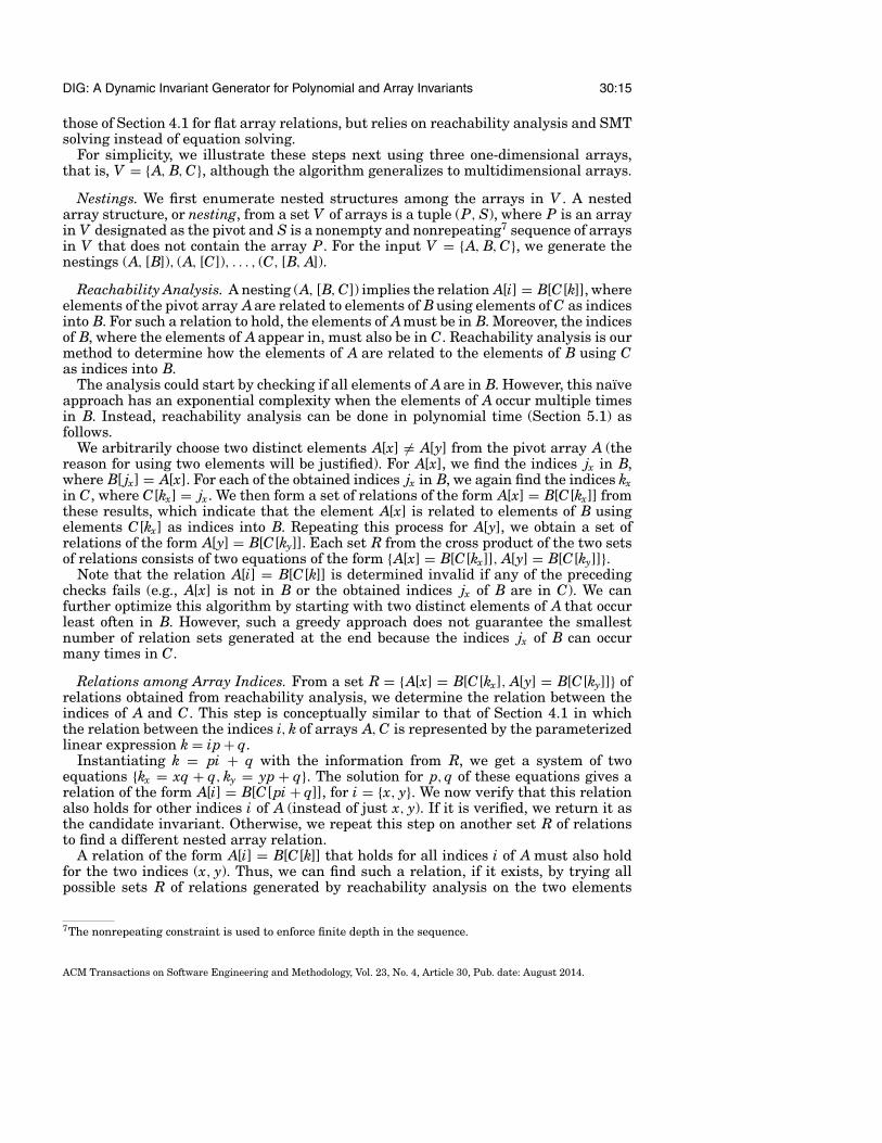
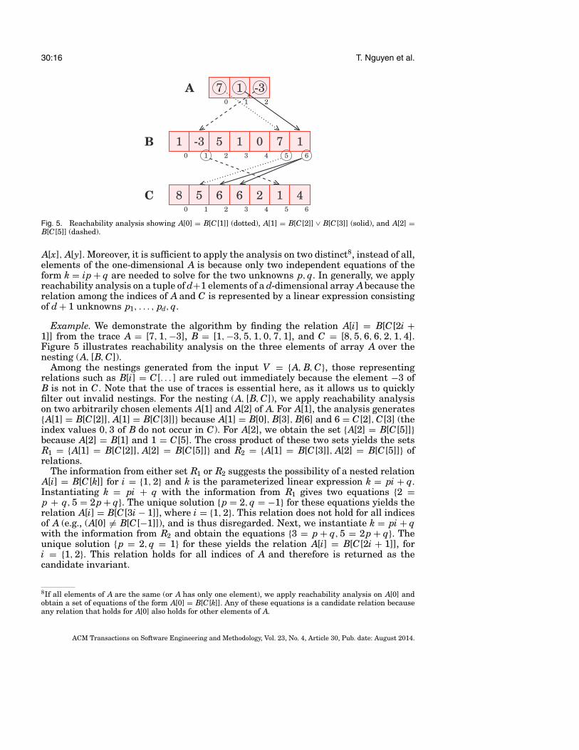
Fig. 5. Reachability analysis showing A[0] = B[C[1]] (dotted), A[1] = B[C[2]] _∨ B[C[3]] (solid), and A[2] =B[C[5]] (dashed).
A[x], A[y]. Moreover, it is sufficient to apply the analysis on two distinct8, instead of all,elements of the one-dimensional A is because only two independent equations of theform k = ip + q are needed to solve for the two unknowns p, q. In generally, we applyreachability analysis on a tuple of d+1 elements of a d-dimensional array Abecause therelation among the indices of A and C is represented by a linear expression consistingof d + 1 unknowns p1, . . . , pd, q.
Example. We demonstrate the algorithm by finding the relation A[i] = B[C[2i +1]] from the trace A = [7, 1,¡−3], B = [1,¡−3, 5, 1, 0, 7, 1], and C = [8, 5, 6, 6, 2, 1, 4].Figure 5 illustrates reachability analysis on the three elements of array A over thenesting (A, [B, C]).
Among the nestings generated from the input V = {A, B, C}, those representingrelations such as B[i] = C[. . . ] are ruled out immediately because the element ¡−3 ofB is not in C. Note that the use of traces is essential here, as it allows us to quicklyfilter out invalid nestings. For the nesting (A, [B, C]), we apply reachability analysison two arbitrarily chosen elements A[1] and A[2] of A. For A[1], the analysis generates{A[1] = B[C[2]], A[1] = B[C[3]]} because A[1] = B[0], B[3], B[6] and 6 = C[2], C[3] (theindex values 0, 3 of B do not occur in C). For A[2], we obtain the set {A[2] = B[C[5]]}because A[2] = B[1] and 1 = C[5]. The cross product of these two sets yields the setsR1 = {A[1] = B[C[2]], A[2] = B[C[5]]} and R2 = {A[1] = B[C[3]], A[2] = B[C[5]]} ofrelations.
The information from either set R1 or R2 suggests the possibility of a nested relationA[i] = B[C[k]] for i = {1, 2} and k is the parameterized linear expression k = pi + q.Instantiating k = pi + q with the information from R1 gives two equations {2 =p + q, 5 = 2p + q}. The unique solution {p = 2, q = ¡−1} for these equations yields therelation A[i] = B[C[3i ¡− 1]], where i = {1, 2}. This relation does not hold for all indicesof A (e.g., (A[0] 6= B[C[¡−1]]), and is thus disregarded. Next, we instantiate k = pi + qwith the information from R2 and obtain the equations {3 = p + q, 5 = 2p + q}. Theunique solution {p = 2, q = 1} for these yields the relation A[i] = B[C[2i + 1]], fori = {1, 2}. This relation holds for all indices of A and therefore is returned as thecandidate invariant.
8If all elements of A are the same (or A has only one element), we apply reachability analysis on A[0] andobtain a set of equations of the form A[0] = B[C[k]]. Any of these equations is a candidate relation becauseany relation that holds for A[0] also holds for other elements of A.
ACM Transactions on Software Engineering and Methodology, Vol. 23, No. 4, Article 30, Pub. date: August 2014.
DIG: A Dynamic Invariant Generator for Polynomial and Array Invariants 30:17
Satisfiability Problem Formulation. In practice, arrays often have large sizes withmultiple duplicate elements, causing reachability analysis to generate many sets R ofrelations to be solved for. Hence, we encode the results of reachability analysis as asatisfiability formula in the theory of linear integer arithmetic, which can be solvedefficiently with modern SMT technologies [Dutertre and De Moura 2006].
Returning to the running example, we create a clause consisting of two atoms (2 =p + q _∨ 3 = p + q) to represent the result {A[1] = B[C[2], A[1] = B[C[3]]} fromreachability analysis. Similarly, the atom 5 = 2p + q is created for {A[2] = B[C[5]]}.Since the relation should hold for the two chosen elements of A, that is, A[i] = B[C[pi +q]] for i = {1, 2}, we combine these formulas into the final CNF formula f = (2 =p+ q _∨ 3 = p + q) ^∧ (5 = 2p + q). Next, we query the SMT solver to return, if possible,an assignment of integers (since array indices are integers) to the variables p and qthat satisfies f . In this example, the solver might assign p = 3, q = ¡−1 for f , whichimplies the relation A[i] = B[C[3i ¡− 1]] for i = {1, 2}. This relation cannot be verifiedbecause it does not hold for all indices of A (e.g., A[0] 6= B[C[¡−1]]). We then add theconstraint ¬(p = 3 ^∧ q = ¡−1) to f and query the SMT solver for a new assignment forp, q. The solver now assigns p = 2, q = 1, implying the relation A[i] = B[C[2i + 1]].This relation is verified to hold for all indices of Aand thus is returned as the candidateinvariant.
We can avoid having to verify each relation by applying the analysis on all elementsof A. Doing so for the running example results in the CNF f = (1 = q) ^∧ (2 = p + q_∨3 =p + q) ^∧ (5 = 2p + q) (the atom 1 = q represents the relation A[0] = B[C[1]], asillustrated in Figure 5). The solution {p = 2, q = 1}, returned by the SMT solver onthe formula f , implies the similar relation A[i] = B[C[2i + 1]] as before. Moreover,this relation is valid for all elements of A because the analysis is applied on all ofthose elements. Thus, we only need to invoke the solver once, but over a more complexformula f (the number of clauses in f is the size of A).
The problem of finding nested array relations has a polynomial-time complexity (bythe algorithm and the analysis given in Section 5.1). However, our implementation inDIG for nested array relations involves SMT technologies and hence does not guaranteea polynomial runtime.9 The experimental results on finding nested arrays in Section 6were obtained when applying reachability analysis on all elements of A.
4.3. Functions
Array invariants involving user-defined functions, for example, A[i] = f (C[i], g(D[i])),require special treatment. We view a function f with n arguments as an n-dimensional array F, where the element F[i1] . . . [in] contains the output of f (i1, . . . , in).Thus, if f is the mult function, then F[4][7] = F[7][4] = 28. For efficiency, Fis represented as a partial array that stores only observed values. For example,if A = [4, 7] and B = [5] are considered, then F contains just the elementsF[4][4], F[4][5], F[4][7], . . . , F[7][7]. Our approach extends to invariants involvingfunction composition, such as g( f (A[. . . ], B[. . . ])). For instance, if g is mod2 which mapseven and odd inputs to 0 and 1 respectively, then the corresponding array G has as itsindices the elements of A, B, F (e.g., G[4] = G[28] = 0, G[5] = G[7] = 1). Just like witharray nesting, we enforce finite depth in nested expressions by disallowing a functionto appear in the scope of one of its arguments, for example, g(f (g(. . . ), f (. . . ))) is notallowed.
DIG predefines a set of basic functions such as mult,add,xor,mod,. . . and automaticallygenerates the corresponding partial arrays based on given traces, as previously. Once
9This depends on the technique implemented in SMT solvers for satisfiability checking over CNFs of thediscussed form.
ACM Transactions on Software Engineering and Methodology, Vol. 23, No. 4, Article 30, Pub. date: August 2014.

30:18 T. Nguyen et al.
Table I. Time Complexity of Invariant Generation Algorithmsin DIG
Invariant Type Form ComplexityEquality (1) O(|T |3)
Polynomial (general) inequality (2) O(|X||T |2 )
Octagonal inequality (3) O(|X||T |2)Flat array relation (4) O(|E|3)Nested array relation (5) O(|X||V |!|E|d|V |)
Note: For polynomial invariants, T represents the set of termsand X the set of traces. For array invariants, V represents theset of array variables, E the set of array elements, d the highestarray dimension among the arrays in V .
functions are included as arrays, DIG can then generate invariants involving functions,such as the nested array relation R[i] = T (mod255(add(L(A[i]), L(B[i])))) in the multWordfunction in AES.
5. ANALYSIS
We first give the computational complexity of DIG’s algorithms for generating differentforms of invariants. Next we show that the polyhedral method generates precise in-equality invariants but can also give many spurious results if the program invariantsdo not appear in the traces.
5.1. Complexity
Table I summarizes the time complexity of DIG’s algorithms for generating invariantsof different forms. The filtering technique in Section 2.3 takes O(|X||T |) to instantiateand check a candidate invariant with |T | terms over |X| traces.
5.1.1. Polynomial Invariants. We analyze the complexity of the algorithms for generatingpolynomial invariants in the number of traces |X| and terms |T |. Recall that terms areused to represent polynomials over variables (Section 2.2). Given a set V of variablesand a degree d, the set T of terms representing monomials over V up to degree dhas size
�|V |+dd
�. The number of terms thus increases exponentially in the number of
variables and degrees.For equalities of the form given in Eq. (1), a standard equation solver is used to
find equality invariants in Section 3.1. We use the traces in X to instantiate |T | inde-pendent equations. The complexity of using Gaussian elimination to solve |T | linearequations for |T | unknowns is O(|T |3) [Farebrother 1988]. Hence, generating invari-ants representing equations among |T | terms takes O(|T |3), cubic in the number ofterms.
In practice, the number of traces often exceeds the number of terms, that is, |X| À |T |,which is desirable because the complexity depends on the smaller parameter |T |. Thecurrent implementation of DIG uses a small random subset of the input traces togenerate equations among terms.
For general inequalities of the form given in Eq. (2), we build polyhedra inSection 3.2.1 to obtain polyhedral (general) inequalities. Constructing a convex poly-hedron over |X| points in |T | dimensions has a theoretical exponential upper bound2(|X|b |T |
2 c) [de Berg et al. 1997]. Thus, the cost of generating polyhedral inequalitiesis O(|X| |T |
2 ), exponential in the number of terms (because a term is essentially a newvariable representing a new dimension).
If one is interested only in inequalities among a fixed number c of terms over programvariables, then the heuristic described in Section 3.2.1 builds polyhedra for all term
ACM Transactions on Software Engineering and Methodology, Vol. 23, No. 4, Article 30, Pub. date: August 2014.
DIG: A Dynamic Invariant Generator for Polynomial and Array Invariants 30:19
combinations of size |c|. The complexity of such a heuristic is O(�|T |
c
�|X||c|), which is
polynomial in |X| and |T | because c is fixed.For octagonal inequalities of the form given in Eq. (3) representing relations between
two terms, we instantiate each pair of terms with the traces in X to obtain the set of |X|points in two dimensions and apply the min, max operations on these points as shownin Section 3.2.2. These two operations run in linear time in |X|, thus identifying theoctagonal constraints for each pair of terms takes O(|X|). There are O(|T |2) such pairsfrom the set of terms T , hence generating octagonal constraints for all pairs of termstakes O(|X||T |2).
5.1.2. Array Invariants. The complexity of the algorithms for generating array invariantsis analyzed in terms of the number of traces |X|, array variables |V |, array elements|E| consisting of elements from all arrays in A, and the highest dimension d among thearrays.
The complexity of the algorithm to find flat array relations of the form given inEq. (4) is dominated by solving equations. As described in Section 4.1, we create |E|new variables to represent array elements and use the equation solving technique inSection 3.1 to find equalities among them. As previously analyzed, generating equali-ties among these variables (terms) takes O(|E|3), the time of solving |E| equations for|E| unknowns.
For nested array relations of the form given in Eq. (5), reachability analysis is appliedon the |V |! nestings enumerated among the arrays in V . For a nesting representingthe relation A[i] = B1[. . . [Bl[ip + q]] . . . ], we apply the analysis on two arbitrarilychosen elements A[ix], A[iy] of the one-dimensional array A. In the worst case, A[ix]could occur O(|B1|) times at B1. Each index value of these O(|B1|) locations could againoccur O(|B2|) times at B2. Thus, the analysis generates O(|B1| · · · |Bl|) relations of theform A[ix] = B1[. . . [Bl[ix p + q]] . . . ] at Bl. This is O(|E||V |), because |Bi| < |E| andl < |V |. Similarly, we obtain O(|E||V |) relations for A[iy]. The cross product of thesetwo sets results in O(|E|2|V |) sets of relations, each set has two equations and twounknowns. More generally, we apply the analysis on d+ 1 elements of a d-dimensionalA and thus obtain O(|E|d|V |) sets of relations. Observe that we obtain O(|A||E||V |) setsof relations if the analysis is applied on all elements of |A| and thus the algorithmbecomes exponential in the number of array elements (|A| = O(|E|)).
From each set of relations, a system of d + 1 equations is instantiated and solved forthe d+1 unknowns to find relations among array indices. Doing this for O(|E|d|v|) sets ofrelations takes O(d3|E|d|v|), which becomes O(|E|d|v|+3) since |E| ¸≥ d. Finally, assumingarray indexing is O(1), the verification that a nested relation A[i] = B1[. . . [Bl[k]] . . . ]holds for all indices of A takes O(l|A|). To be comprehensive, we check the candidaterelation over the traces in X and hence verification takes O(l|A||X|).
The algorithm given in Section 4.2 is thus O(l|A||X||V |!|E|d|V |+3), which isO(|X||V |!|E|d|V |+3), because |E| > l|A|. Moreover, we can fix |V | and d because, inpractice, the number of array elements is typically much larger than the number ofarrays or the array dimensions. Hence, the complexity of finding nested array relationsis polynomial in the number of array elements |E|.
5.2. Polyhedra and Inequalities
The polyhedral method described in Section 3.2.1 merits additional discussion becauseit generates precise inequalities that guaranteed to underapproximate the desiredinvariants10 expressible under the considered inequality forms. However, if the desired
10Desired invariants refer to program invariants, that is, relations that are guaranteed to hold at a programlocation for all possible traces observed at that location.
ACM Transactions on Software Engineering and Methodology, Vol. 23, No. 4, Article 30, Pub. date: August 2014.
30:20 T. Nguyen et al.
invariants do not fall under the considered forms, this method could generate a complexpolyhedron whose facets represent many spurious invariants.
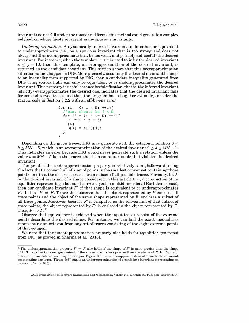
Underapproximation. A dynamically inferred invariant could either be equivalentto underapproximate (i.e., be a spurious invariant that is too strong and does notalways hold) or overapproximate (i.e., be too weak and possibly not useful) the desiredinvariant. For instance, when the template x ≤ y is used to infer the desired invariantx ≤ y ¡− 10, then this template, an overapproximation of the desired invariant, isreturned as the candidate invariant. This section shows that this overapproximationsituation cannot happen in DIG. More precisely, assuming the desired invariant belongsto an inequality form supported by DIG, then a candidate inequality generated fromDIG using convex hulls can only be equivalent to or underapproximates the desiredinvariant. This property is useful because its falsification, that is, the inferred invariant(strictly) overapproximates the desired one, indicates that the desired invariant failsfor some observed traces and thus the program has a bug. For example, consider theflatten code in Section 3.2.2 with an off-by-one error.
for (i = 0; i < M; ++i){//bug, should be j < Nfor (j = 0; j <= N; ++j){
k = i * n + j;[L]B[k] = A[i][j];
}}
Depending on the given traces, DIG may generate at L the octagonal relation 0 ≤k ≤ MN + 5, which is an overapproximation of the desired invariant 0 ≤ k ≤ MN ¡− 1.This indicates an error because DIG would never generate such a relation unless thevalue k = MN + 5 is in the traces, that is, a counterexample that violates the desiredinvariant.
The proof of the underapproximation property is relatively straightforward, usingthe facts that a convex hull of a set of points is the smallest convex set containing thosepoints and that the observed traces are a subset of all possible traces. Formally, let Fbe the desired invariant of a shape considered in this article (i.e., a conjunction of in-equalities representing a bounded convex object in multidimensional Euclidean space),then our candidate invariant F 0 of that shape is equivalent to or underapproximatesF, that is, F 0 )⇒ F. To see this, observe that the object represented by F encloses alltrace points and the object of the same shape represented by F 0 encloses a subset ofall trace points. Moreover, because F 0 is computed as the convex hull of that subset oftrace points, the object represented by F 0 is enclosed in the object represented by F.Thus, F 0 )⇒ F.11
Observe that equivalence is achieved when the input traces consist of the extremepoints describing the desired shape. For instance, we can find the exact inequalitiesrepresenting an octagon from any set of traces consisting of the eight extreme pointsof that octagon.
We note that the underapproximation property also holds for equalities generatedfrom DIG, as proved in Sharma et al. [2013].
11The underapproximation property F 0 )⇒ F also holds if the shape of F 0 is more precise than the shapeof F. This property is not guaranteed if the shape of F 0 is less precise than the shape of F. In Figure 3,a desired invariant representing an octagon (Figure 3(c)) is an overapproximation of a candidate invariantrepresenting a polygon (Figure 3(d)) and is an underapproximation of a candidate invariant representing aninterval (Figure 3(b)).
ACM Transactions on Software Engineering and Methodology, Vol. 23, No. 4, Article 30, Pub. date: August 2014.
DIG: A Dynamic Invariant Generator for Polynomial and Array Invariants 30:21
Spurious Invariants. The polyhedral method has a high theoretical complexity be-cause it could produce a complex polyhedron with multiple facets in high dimensionsdepending on the given trace points. Importantly, if the traces do not precisely capturethe desired invariant, then the polyhedron consists of many facets representing spuri-ous inequalities. For instance, if x, y can take any value over the reals, then an n-facetpolygon computed over any set of traces for x, y produces n spurious invariants becauseno bounded polygons can capture the unbounded ranges of x, y.
Although filtering (Section 2.3) reduces spurious invariants by removing facets of thepolyhedron (i.e., widening it), the modified polyhedron can still have many remainingfacets representing faux relations because it is rare to have inequalities among allinvolved terms. Thus, DIG does not automatically invoke the polyhedral method forgeneral inequalities. The method is effective when the user has certain expectationsabout the desired invariants. The user can ask DIG for octagonal relations if onlyinequalities among pairs of terms over program variables are of interest. The user canalso hypothesize a spherical shape c1x2 + c2y2 +c 3z2 and query DIG to search for thatexact sphere (i.e., compute the coefficients ci) from the convex hull built over tracepoints for these terms. The availability of source code allows for hybrid approacheswith static analysis such as slicing [Reps et al. 1995] to automatically find variablesthat are likely related to one another, reducing the number of term combinations.
In contrast to the convex hull construction, methods using equation solving give fewspurious equalities, because equalities are stricter constraints than inequalities. Forexample, we can always compute a convex polygon representing many inequalities overany set of finite points in 2D, but can only have at most a line representing an equal-ity over these points. Moreover, assuming traces are obtained from random programinputs, it is unlikely that a large set of traces would exhibit random false equalities.The next section shows that DIG does not generate spurious equality relations for bothnumerical and array variables in our experiments.
6. EXPERIMENTAL RESULTS
Our prototype, DIG, is implemented in Python using the Sage mathematical environ-ment [Stein 2012]. The prototype uses built-in Sage functions to solve equations andconstruct polyhedra. It also uses Z3 [De Moura and Bjørner 2008] to check the satisfi-ability of SMT formulas. The experiments reported here were performed on dual-core2.3GHz Intel Unix-based system with 8GB of RAM.
6.1. Programs
We evaluated DIG on programs taken from a test suite which we call NLA (nonlineararithmetic) and an implementation of the Advanced Encryption Standard (AES)[Rijmen and Daemen 2001]. The details of NLA and AES are given in Tables II and III,respectively.
The NLA test suite consists of 27 programs from various sources collected byRodrıguez-Carbonell and Kapur [Carbonell and Kapur 2007a, 2007b; Carbonell 2006].These programs implement classic arithmetic algorithms that are widely used in pro-gramming, such as mult, div, mod, sqrt, gcd. The programs are relatively small, about20 lines of C code each. However, they implement nontrivial mathematical algorithmsand are often used to benchmark static analysis methods. Importantly, the complexityof our method depends on the size of the traces and the invariant forms of interest—not the size of the program per se. Among the 27 programs from NLA, there are 41documented nonlinear relations: 39 equations and 2 inequalities.
The second benchmark, AES, is an annotated AES implementation from Yin et al.[2009]. It exemplifies a real-world security-critical application and contains nontriv-ial array invariants. To show that the implementation conform to the formal AES
ACM Transactions on Software Engineering and Methodology, Vol. 23, No. 4, Article 30, Pub. date: August 2014.
30:22 T. Nguyen et al.
specification, the authors of AES inspected and documented the invariants of eachfunction in AES and then fully verified the result using SPARK Ada [Barnes 2003]and PVS [Owre et al. 1992]. The annotated invariants represent the manual effortrequired to fully verify the functionality of an AES implementation using axiomaticsemantics. AES contains 868 lines of Ada code organized into 25 functions containing30 invariants: 8 flat array relations, 7 nested array relations, 2 linear equations, and13 other relations.
Program Locations and Execution Traces. Our test programs come with documentedinvariants at various locations such as loop heads and function exits. For evaluationpurpose, we find invariants at those locations automatically and compare them to thehuman-documented invariants. We manually instrumented the program source code totrace values of all variables in the scope at each program location containing a knowninvariant. Specifically, for NLA, invariants are obtained mainly at loop entrances. ForAES, invariants are obtained mainly at function exits. For NLA, it turns out that mostof the loop invariants specify the behaviors of the programs (e.g., the egcd programin Figure 1 and cohen in Figure 4). In addition, we apply DIG over traces captured atsystematically chosen program locations (e.g., all function entries) and verify its resultsat these locations manually.
The instrumented programs were run against a set of randomly selected inputs. Thenumber of obtained traces is different across programs and program locations. Forexample, locations inside loops may be visited many times while function exits may bevisited rarely. DIG automatically selects a set of random traces whose size is 1.5 timesthe number of created terms for invariant generation and another set of 1,000 randomtraces for filtering.
6.2. Quality of Results
DIG selects the appropriate algorithms for finding invariants depending on the vari-ables that appear in the trace file. For numerical variables, DIG first generates equali-ties among terms, and next proceeds to inequalities using the deduction method whenadditional information such as loop guards is available. By default, we do not gener-ate inequalities using the convex hull methods unless specified by the user. For arrayvariables, DIG first generates flat relations and then nested relations. For invariantsinvolving user-defined functions, this information must be specified by the user be-cause it is not available from traces. The post-processing step refines the candidateinvariants when each invariant generation algorithm finishes.
For the experiments reported here, we define a single parameter, ®α = 200 whichbounds DIG’s running times. For polynomial invariants, DIG automatically adjuststhe maximum degree so that the number of generated terms does not exceed ®α. For flatarray relations, DIG automatically adjusts the sizes of the considered arrays in such away that the total number of array elements does not exceed ®α. There is no parameterfor nested array relations because reachability analysis enumerates all possible non-repeating nestings to consider array relations up to any nesting depth.
6.2.1. NLA. Table II reports experimental results on 27 programs from NLA, with run-ning times averaged over 20 runs. The Invs column reports the number of nonlinearinvariants generated by DIG and their types (equality or inequality). The V, D columnreports the number of distinct variables (a subset of the considered variables) and thehighest polynomial degree in the generated invariants. The T®α column reports the av-erage time in seconds to discover the invariants using parameter ®α, including the timeto refine the results. The Td eg column reports the average time in seconds to discoverthese invariants if we had restricted the search space to the polynomial degree givenin the V, D column. The Vs Doc column reports the number of documented invariants
ACM Transactions on Software Engineering and Methodology, Vol. 23, No. 4, Article 30, Pub. date: August 2014.

DIG: A Dynamic Invariant Generator for Polynomial and Array Invariants 30:23
Table II. Experimental Results on 27 Programs from NLA
Program Desc Invs V, D T®α Tdeg Vs Docdivbin div 1 eq 5, 2 27.0 0.3 1/1cohendiv div 2 eq, 2 ieq 6, 2 8.5 0.8 3/3mannadiv int div 1 eq 5, 2 23.1 1.0 1/1hard int div 2 eq 6, 2 9.2 0.9 2/2sqrt1 square root 2 eq, 2 ieq 4, 2 39.6 0.9 3/3dijkstra square root 4 eq 5, 3 31.4 4.0 1/1freire1 square root 1 eq 3, 2 33.9 0.2 1/1freire2 cubic root 4 eq 4, 2 45.5 2.9 2/2cohencube cubic sum 3 eq 5, 3 39.5 8.4 3/3egcd gcd 3 eq 8, 2 53.9 2.2 2/2egcd2 gcd 3 eq 10, 2 4.2 4.5 3/3egcd3 gcd 4 eq 12, 2 8.2 8.8 4/4lcm1 gcd, lcm 1 eq 6, 2 8.7 0.5 1/1lcm2 gcd, lcm 1 eq 6, 2 11.5 0.7 1/1prodbin product 1 eq 5, 2 32.5 0.4 1/1prod4br product 1 eq 6, 3 8.2 8.5 1/1fermat1 divisor 1 eq 5, 2 31.6 0.4 1/1fermat2 divisor 1 eq 5, 2 31.6 0.4 1/1knuth divisor 4 eq 8, 3 53.8 53.8 1/1geo1 geo series 1 eq 4, 2 14.8 0.1 1/1geo2 geo series 1 eq 4, 2 24.4 0.1 1/1geo3 geo series 1 eq 5, 3 23.4 2.4 1/1ps2 pow sum 1 eq 3, 2 29.2 0.2 1/1ps3 pow sum 1 eq 3, 3 27.9 0.3 1/1ps4 pow sum 1 eq 3, 4 29.7 0.8 1/1ps5 pow sum 1 eq 3, 5 30.2 2.8 1/1ps6 pow sum 1 eq 3, 6 28.2 8.5 1/127 programs 52 invs 709.2s 114.7s 41/41
matched by our results. For example, DIG generated four quadratic relations (twoequalities and two inequalities) over six variables for cohendiv in 8.5s (or 0.8s if themaximum degree 2 was specified). The obtained invariants also match with the threedocumented invariants.
To evaluate DIG, we compared its results to the documented invariants or verifiedthem manually against the program source code. Comparing to the documented invari-ants, DIG found all 41 documented relations from the 27 programs in NLA. In mostcases, the results matched the documented invariants exactly as written. Occasionallywe achieved results that are mathematically equivalent to the documented invariants.For example, sqrt1 has two documented equalities 2a + 1 = t, (a + 1)2 = s; our resultsgave 2a + 1 = t, t2 + 2t + 1 = 4s, which is equivalent to (a + 1)2 = s by substituting twith 2a+1. In many cases, DIG discovered undocumented invariants, for example, therelation 1 = im¡− jk in the example program egcd in Section 2. We also found invariantsthat are stronger than the documented ones, for example, the two quadratic relationsdiscovered in freire2 imply a documented relation of degree 3 (DIG also found thiscubic invariant but automatically pruned it in post processing because it is weakerthan the other two). We obtained no spurious results for NLA using the method basedon equation solving. We believe and intend to formally prove that our method for gen-erating equality invariants has this desirable property. That is, assuming random andadequate traces (e.g., ¸≥ n unique traces for n unknowns), the method will generate onlytrue equality invariants. Note that this property will not hold for inequalities, because
ACM Transactions on Software Engineering and Methodology, Vol. 23, No. 4, Article 30, Pub. date: August 2014.
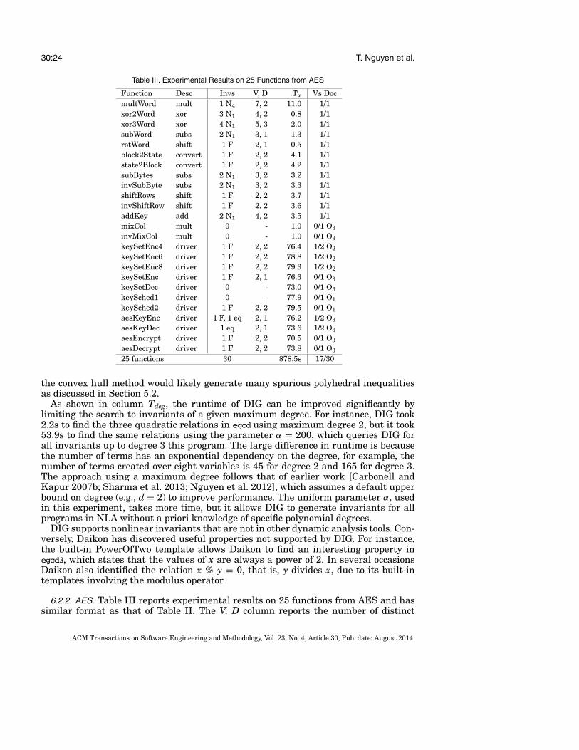
30:24 T. Nguyen et al.
Table III. Experimental Results on 25 Functions from AES
Function Desc Invs V, D T®α Vs DocmultWord mult 1 N4 7, 2 11.0 1/1xor2Word xor 3 N1 4, 2 0.8 1/1xor3Word xor 4 N1 5, 3 2.0 1/1subWord subs 2 N1 3, 1 1.3 1/1rotWord shift 1 F 2, 1 0.5 1/1block2State convert 1 F 2, 2 4.1 1/1state2Block convert 1 F 2, 2 4.2 1/1subBytes subs 2 N1 3, 2 3.2 1/1invSubByte subs 2 N1 3, 2 3.3 1/1shiftRows shift 1 F 2, 2 3.7 1/1invShiftRow shift 1 F 2, 2 3.6 1/1addKey add 2 N1 4, 2 3.5 1/1mixCol mult 0 - 1.0 0/1 O3invMixCol mult 0 - 1.0 0/1 O3keySetEnc4 driver 1 F 2, 2 76.4 1/2 O2keySetEnc6 driver 1 F 2, 2 78.8 1/2 O2keySetEnc8 driver 1 F 2, 2 79.3 1/2 O2keySetEnc driver 1 F 2, 1 76.3 0/1 O3keySetDec driver 0 - 73.0 0/1 O3keySched1 driver 0 - 77.9 0/1 O1keySched2 driver 1 F 2, 2 79.5 0/1 O1aesKeyEnc driver 1 F, 1 eq 2, 1 76.2 1/2 O3aesKeyDec driver 1 eq 2, 1 73.6 1/2 O3aesEncrypt driver 1 F 2, 2 70.5 0/1 O3aesDecrypt driver 1 F 2, 2 73.8 0/1 O3
25 functions 30 878.5s 17/30
the convex hull method would likely generate many spurious polyhedral inequalitiesas discussed in Section 5.2.
As shown in column Tdeg, the runtime of DIG can be improved significantly bylimiting the search to invariants of a given maximum degree. For instance, DIG took2.2s to find the three quadratic relations in egcd using maximum degree 2, but it took53.9s to find the same relations using the parameter ®α = 200, which queries DIG forall invariants up to degree 3 this program. The large difference in runtime is becausethe number of terms has an exponential dependency on the degree, for example, thenumber of terms created over eight variables is 45 for degree 2 and 165 for degree 3.The approach using a maximum degree follows that of earlier work [Carbonell andKapur 2007b; Sharma et al. 2013; Nguyen et al. 2012], which assumes a default upperbound on degree (e.g., d = 2) to improve performance. The uniform parameter ®α, usedin this experiment, takes more time, but it allows DIG to generate invariants for allprograms in NLA without a priori knowledge of specific polynomial degrees.
DIG supports nonlinear invariants that are not in other dynamic analysis tools. Con-versely, Daikon has discovered useful properties not supported by DIG. For instance,the built-in PowerOfTwo template allows Daikon to find an interesting property inegcd3, which states that the values of x are always a power of 2. In several occasionsDaikon also identified the relation x % y = 0, that is, y divides x, due to its built-intemplates involving the modulus operator.
6.2.2. AES. Table III reports experimental results on 25 functions from AES and hassimilar format as that of Table II. The V, D column reports the number of distinct
ACM Transactions on Software Engineering and Methodology, Vol. 23, No. 4, Article 30, Pub. date: August 2014.

DIG: A Dynamic Invariant Generator for Polynomial and Array Invariants 30:25
array variables and the highest dimension of the arrays in the candidate invariants.The types of the generated invariants, reported in the Invs columns, include Flat,Nested, and linear equality invariants (Nl indicates that the depth of the generatednested array relation is l). The Vs Doc column also indicates the types of documentedinvariant (called Others) that DIG could not identify. The driver functions are composedfrom other functions in this table.
DIG discovered 30 candidate invariants for AES, all of which are valid relations,using the parameter ®α = 200 as in the NLA experiment. Comparing to the documentedinvariants, we found all 17 documented relations that are expressible in the consideredforms. In many cases, DIG also discovered undocumented invariants. In the threerelations r[i] = xor(a[i], b[i]), a[i] = xor(r[i], b[i]), b[i] = xor(r[i], a[i]) obtained fromxor2Word, the first one is a documented invariant but the other two are indeed propertiesof the xor operator. In addition to the documented invariant r[i][ j] = S[t[i][ j]] insubWord, we found the relation t[i][ j] = Si[r[i][ j]], which is valid because the array Sicontains the reversed values of the array S. The results generated for the keySetupEncfunctions are conditional invariants, for example, in keySetupEnc8, we got r[i][ j] =k[4i + j] for i = 0, . . . , 7, j = 0, . . . , 3 and r[i][ j] = 0 for other indices i, j. In severalcases, the algorithms for both flat and nested array relations discover similar invariantssuch as S[i][ j] = R[4i + j] in state2Block because these flat array relations are alsonested array relations with nesting depth 0. We did not obtain spurious invariants forthe functions in AES.
Similar to NLA, DIG’s runtime for AES can be significantly improved with someadditional information about the desired invariants. For instance, DIG found the rela-tion t[i][ j] = c[4i + j] in aesDecrypt under 10s using reachability analysis but over 60susing the algorithm for flat array relations (for solving 200 equations). The last elevenfunctions in Table III has similar run times (77s on average) because the consideredarrays in each function were automatically resized to contain ®α = 200 elements. Wenote that a smaller parameter value is also sufficient to obtain similar results for AESwith much shorter runtime, for example, DIG took on average 14.3s for the last elevenfunctions when run with ®α = 50.
The 13 documented invariants that were not discovered fall into categories thatare not supported by DIG and are left for future work. These can be grouped intothree categories: Others1¡−3. Others1 includes nested array relations such as A[i] =4B[6C[. . . ]]. We do not currently handle nested invariants if the elements of A are notexactly nested in B. Others2 includes nested array invariants such as A[i] = B[C[. . . ]]and A[ j] = B[C[. . . ]], where i 6= j, that is, a conditional form of nested array relations.We require that generated relations such as A[i] = B[C[. . . ]] hold for all i. Others3includes array invariants involving functions whose inputs are arrays, such as f ([1, 2]).We only consider functions with scalar inputs such as g(7, 8). We note that existingdynamic analysis methods cannot find these array relations either.
The manual annotation of AES with sufficient invariants to admit machine-checkedfull formal verification was a significant undertaking involving hours of tool-assistedmanual effort [Yin et al. 2009, 2008]. Annotating pre- and post-conditions and loopinvariants has not been solved in general and is known to be a key bottleneck inapproaches based on axiomatic semantics [Flanagan and Leino 2001]. It is not sur-prising that our approach was unable to discover all relevant invariants; indeed,we view reducing the manual verification annotation burden by one-half as a strongresult.
6.2.3. Other Program Locations. DIG can be applied over traces captured at arbitrarylocations, including those with invariants that are not currently considered or thosethat do not likely have useful invariants. Table III shows that DIG generated ten valid
ACM Transactions on Software Engineering and Methodology, Vol. 23, No. 4, Article 30, Pub. date: August 2014.

30:26 T. Nguyen et al.
invariants and no spurious results when applied to locations in AES with invariantsunder the unsupported forms Others1¡−3. When being applied to systematicallychosen locations like all program entry points in NLA, DIG generates no invariantsbecause these programs take in random input values, for example, ¡−1∞ ≤ x ≤ 1∞ (anunsupported form of invariant that cannot be captured by finite traces). Note thatif we had used the convex hull methods to generate inequalities, then we will getspurious relations such as c1 ≤ x ≤ c2, where c1, c2 correspond to the lower and upperbounds of x from the input traces. In general, we expect DIG’s candidate invariants atarbitrary locations from any program to have similar quality as those reported here(these invariants were obtained without a priori knowledge about their forms).
To summarize, DIG found all of the invariants under consideration: 100% of thedocumented nonlinear invariants in NLA and 17 out of 30 documented invariants inAES. The other 13 invariants were beyond the scope of this article and are left for futurework. To the best of our knowledge, no other dynamic invariant analysis approacheshave analyzed the forms of invariants discussed in this article.
6.3. Limitations
Two of the operations, namely, reachability analysis and polyhedra construction, areexpensive, because the analysis can generate many relation sets over large arrays andmany inequalities representing complex polyhedra in high dimensions. We addressthese issues using SMT solvers by deducing new inequalities through loop conditions, orby generating simpler invariants by building octagons. Nonetheless, these techniqueshave trade-offs: having high theoretical complexities, requiring additional information,or loosing precisions by representing invariants with simpler shapes.
Floating point values are subject to round-off errors that may confound some exactchecks. Given an abundance of available traces, we filter out certain traces containingrounded float values. DIG also allows comparison within "ε instead of exact comparisons(e.g., 0.33333 ¼≈ 1
3 and 0.99998 ¼≈ 1.0). The use of established techniques from numericalanalysis to handle other corner cases in floating point arithmetic is left for future work.
As discussed in Section 5.2, the effectiveness of our method depends on programtraces produced by test inputs. DIG cannot derive properties that are not exhibited bythe traces. For example, if the relation x + y > 10, but not x + y = 10, is implicatedby the traces, then we cannot find the inequality x + y ¸≥ 10. We note the existence ofmany active research projects investigating high-coverage test inputs and efficient testsuites. In particular, we can take advantage of an entire body of work on generatingtest suites specifically for dynamic invariant detection [Gupta and Heidepriem 2003;Harder et al. 2003; Xie and Notkin 2003].
Finally, our work focuses on specialized types of invariants. It is unlikely that DIGwill find invariants of other, unrelated forms, as seen in the AES benchmark. We believethat our approach strikes a balance between rich expressive power, allowing it to findmany invariants with real-world uses (e.g., documentation in NLA, verification in AES)and efficiency, allowing it to complete in seconds per program.
7. RELATED WORK
Daikon [Ernst 2000; Ernst et al. 2007; Perkins and Ernst 2004], the paragon of dynamicinvariant analysis, infers candidate invariants from traces and templates. By default,the system reports invariants at the entry and exit points of a function, although itis possible to extract invariants at other locations, such as inside loops, by manualinstrumentation. The system comes with a large list of assorted invariant templatesthat are considered as useful to programmers and allows user-supplied invariants. Forpolynomial relations, the system can find linear relations over at most three variables,
ACM Transactions on Software Engineering and Methodology, Vol. 23, No. 4, Article 30, Pub. date: August 2014.
DIG: A Dynamic Invariant Generator for Polynomial and Array Invariants 30:27
for example, x + 2y ¡− 3z + 4 = 0, and has fixed nonlinear templates such as x = y2.Relations among arrays have limited support in Daikon, for example, the relationsA[i] = B[C[i]], A[i] = 2B[i] + C[5] + 7 are not considered.
There is related work on dynamic methods for finding invariants for debugging (e.g.,the detected properties are used to find certain type of errors). The Diduce [Hangaland Lam 2002] tool analyzes what happens when an error occurs by looking at thedifferences between the previous and current values of variables. Statistical debug-ging [Liblit et al. 2005], a fault localization technique, looks for relations (e.g., {<,=,>})between two variables or a variable and a constant. The Spin model checker [Vaziriand Holzmann 1998] can also find relations over two variables. In general, these ap-proaches find invariants that are relatively simple compared to those given by Daikonand DIG.
Abstract Interpretation [Cousot and Cousot 1976, 1977; Cousot and Halbwachs 1978]is a popular framework in static invariant analysis that approximates program prop-erties under a given domain, for example, the polyhedra domain expresses generallinear relations over variables. The method starts from an initial approximation andgradually improves the approximation based on the structure of the program until nomore improvements can be made (a fixed-point). A widening heuristic operator is oftenused to ensure termination.
Carbonell and Kapur [2007; Carbonell 2006] provide an abstract interpretationframework for polynomial equalities of the form given in Eq. (1). They first observethat a set of polynomial invariants form the algebraic structure of an ideal, then com-pute the polynomial invariants using Grobner basis and operations over ideals basedon the structure of the program until a fixed point is reached. Scalability is an issuebecause the approach must consider all possible program paths to guarantee soundresults. The method can analyze precisely only programs with assignments and loopguards expressible as polynomial equalities. To ensure termination when analyzingprograms with nested loop, the method uses a widening operator that depends on apriori bound on the degrees of the polynomials. Carbonell and Kanpur [2007a] does notrequire upperbounds on polynomial degrees but is restricted to non-nested loops. Thiswork does not support the forms of inequalities and array relations in DIG.
Recently, Sharma et al. [2013] proposed a complete and sound approach that hy-bridizes dynamic and static analysis to generate equality invariants. They use the al-gorithm of Section 3.1 to compute equality invariants from traces and use SMT solvingto verify that the candidate invariants are correct with respect to the program sourcecode. Counterexamples to candidate invariants that fail to prove are subsequently usedto produce more traces to generate better candidate invariants. They formally provethat the candidate equalities are sound (i.e., always underapproximate the programinvariant), and the approach terminates after a finite number of steps to generate andverify candidate invariants. It would be interesting if this approach could be extendedto inequality invariants generated by DIG, which are also underapproximations andcan be checked for satisfiability using SMT solvers.
8. CONCLUSION
We present DIG, the first dynamic invariant generator that can discover nonlinearpolynomial and linear array invariants. Our method applies mathematical techniquesnot previously employed to aid dynamic invariant detection. By generating invariantsdirectly based on input traces, our results are very accurate with respect to giventraces. For nonlinear equality relations, we generate terms representing nonlinearpolynomials among variables and use an equation solver to find linear relations amongthe terms; this yields nonlinear relations among the original variables. We represent
ACM Transactions on Software Engineering and Methodology, Vol. 23, No. 4, Article 30, Pub. date: August 2014.
30:28 T. Nguyen et al.
inequality constraints using geometric shapes and reduce the task for inferring gen-eral inequalities to generating convex polyhedra. For nonlinear inequality relations,we generate terms and then build convex polyhedra, obtaining the desired relationsfrom their facets. Building convex polyhedra in high dimensions is expensive, thus, weconsider less expressive forms of inequalities that represent simpler geometric shapes,such as octagons. When additional information, such as a loop entry condition, is avail-able, we can efficiently take advantage of it to deduce new inequalities by combiningdiscovered equality relations with the provided loop condition. For flat array relations,we look for relations among individual array elements and extract from those resultsthe possible relations among the array indices. These flat array relations also expressconditional information, capturing array relations that hold for specific indices. Fornested array relations, we build an SMT query using information obtained from areachability analysis; the satisfying assignment provided by the SMT solver yields thedesired invariant.
Our evaluation demonstrates the feasibility and potential of DIG by successfullyidentifying 100% of the nonlinear invariants in 27 nontrivial algorithms as well as60% of the documented array relations necessary for full formal verification of an AESimplementation.
ACKNOWLEDGMENTS
This work is a continuation of a project initiated by Jack Pullikottil with Deepak Kapur in 2003. We thankMatthias Horbach and Hengjun Zhao for insightful discussions as well as Xiang Yin for providing the AESimplementation.
REFERENCES
J. Barnes. 2003. High Integrity Software: The SPARK Approach to Safety and Security. Addison-WesleyLongman Publishing Co., Inc.
Bruno Blanchet, Patrick Cousot, Radhia Cousot, Jerome Feret, Laurent Mauborgne, Antoine Mine, DavidMonniaux, and Xavier Rival. 2003. A static analyzer for large safety-critical Software. In Proceedings ofthe Conference on Programming Languages Design and Implementation. 196–207.
Rastislav Bodık, Rajiv Gupta, and Vivek Sarkar. 2000. ABCD: Eliminating array bounds checks on demand.In Proceedings of the Conference on Programming Language Design and Implementation. 321–333.
Enric Rodrıguez Carbonell. 2006. Automatic generation of polynomial invariants for system verification.Ph.D. Dissertation, Technical University of Catalonia, Barcelona, Spain.
Enric Rodrıguez Carbonell and Deepak Kapur. 2007a. Generating all polynomial invariants in simple loops.Symbol. Computa. 42, 4 (2007), 443–476. DOI: http://dx.doi.org/10.1016/j.jsc.2007.01.002
Enric Rodrıguez Carbonell and D. Kapur. 2007b. Automatic generation of polynomial invariants of boundeddegree using abstract interpretation. Sci. Comput. Program. 64. (Jan. 2007), 54–75. DOI: http://dx.doi.org/10.1016/j.scico.2006.03.003
Edward Cohen. 1990. Programming in the 1990s: An Introduction to the Calculation of Programs. Springer-Verlag.
P. Cousot and R. Cousot. 1976. Static determination of dynamic properties of programs. In Proceedings ofthe International Symposium on Programming. 106–130.
Patrick Cousot and Radhia Cousot. 1977. Abstract interpretation: A unified lattice model for static analysisof programs by construction or approximation of fixpoints. In Proceedings of the International Synposiumon Principles of Programming Languages. 238–252.
Patrick Cousot, Radhia Cousot, Jerome Feret, Laurent Mauborgne, Antoine Mine, David Monniaux, andXavier Rival. 2005a. The AstrEe analyzer. In Proceedings of the European Symposium on Programming.21–30.
P. Cousot, R. Cousot, J. Feret, L. Mauborgne, A. Mine, D. Monniaux, and X. Rival. 2005b. The Astree analyzer.In Proceedings of the Conference on European Symposium on Programming (ESOP’05). Lecture Notesin Computer Science, vol. 3444, Springer, 21–30.
Patrick Cousot and Nicolas Halbwachs. 1978. Automatic discovery of linear restraints among variables ofa program. In Proceedings of the International Symposium on Principles of Programming Languages.84–96.
ACM Transactions on Software Engineering and Methodology, Vol. 23, No. 4, Article 30, Pub. date: August 2014.
DIG: A Dynamic Invariant Generator for Polynomial and Array Invariants 30:29
Mark de Berg, Marc van Kreveld, Mark Overmars, and Otfried Schwarzkopf. 1997. Computational Geometry:Algorithms and Applications. Springer-Verlag.
Leonardo De Moura and Nikolaj Bjørner. 2008. Z3: An efficient SMT solver. In Tools and Algorithmsfor the Construction and Analysis of Systems, Springer, 337–340. http://research.microsoft.com/en-us/um/redmond/projects/z3/.
Nachum Dershowitz and Zohar Manna. 1978. Inference rules for program annotation. In Proceedings of theInternational Conference on Software Engineering. 158–167.
B. Dutertre and L. De Moura. 2006. A fast linear-arithmetic solver for DPLL(T). In Computer Aided Verifi-cation. Springer, 81–94.
M. D. Ernst. 2000. Dynamically detecting likely program invariants. Ph.D. Dissertation, University ofWashington.
Michael D. Ernst, Jeff H. Perkins, Philip J. Guo, Stephen McCamant, Carlos Pacheco, Matthew S. Tschantz,and Chen Xiao. 2007. The Daikon system for dynamic detection of likely invariants. Sci. Comput.Program. 1–3. (2007), 35–45.
R. W. Farebrother. 1988. Linear Least Squares Computations. Marcel Dekker, Inc.Jerome Feret. 2004. Static analysis of digital filters. In Programming Languages and Systems, Springer,
33–48.Cormac Flanagan and K. Rustan M. Leino. 2001. Houdini, an annotation assistant for ESC/Java. In Proceed-
ings of the Intenational Symposium on Formal Methods for Increasing Software Productivity. 500–517.Steven M. German and Ben Wegbreit. 1975. A synthesizer of inductive assertions. IEEE Trans. Softw. Eng.
1, 1 (1975), 68–75.N. Gupta and Z. V. Heidepriem. 2003. A new structural coverage criterion for dynamic detection of program
invariants. In Proceedings of the International Conference on Automated Software Engineering. 49–58.Sudheendra Hangal and Monica S. Lam. 2002. Tracking down software bugs using automatic anomaly
detection. In Proceedings of the International Conference on Software Engineering. 291–301.M. Harder, J. Mellen, and M. D. Ernst. 2003. Improving test suites via operational abstraction. In Proceedings
of the International Conference on Software Engineering. 60–71.Neil D. Jones, Carsten K. Gomard, and Peter Sestoft. 1993. Partial Evaluation and Automatic Program
Generation. Prentice Hall.Michael Karr. 1976. Affine relationships among variables of a program. Acta Informatica 6 (1976), 133–151.Shmuel Katz and Zohar Manna. 1976. Logical analysis of programs. Commun. ACM 19, 4 (1976), 188–206.Ben Liblit, Mayur Naik, Alice X. Zheng, Alex Aiken, and Michael I. Jordan. 2005. Scalable statistical bug
isolation. In Proceedings of the Conference on Programming Language Design and Implementation.15–26.
Antoine Mine. 2004. Weakly relational numerical abstract domains. Ph.D. Dissertation, Ecole Polytechnique,Palaiseau, France.
ThanhVu Nguyen, Deepak Kapur, Westley Weimer, and Stephanie Forrest. 2012. Using dynamic analysisto discover polynomial and array invariants. In Proceedings of the International Conference on SoftwareEngineering. IEEE, 683–693.
S. Owre, J. Rushby, and N. Shankar. 1992. PVS: A prototype verification system. In Proceedings of the 11thInternational Conference on Automated Deduction (CADE). Lecture Notes in Computer Science, vol. 607,Springer-Verlag, 748–752.
Jeff H. Perkins and Michael D. Ernst. 2004. Efficient incremental algorithms for dynamic detection of likelyinvariants. ACM SIGSOFT Softw. Eng. Notes, 29, 6 (2004), 23–32.
Jeff H. Perkins, Sunghun Kim, Sam Larsen, Saman Amarasinghe, Jonathan Bachrach, Michael Carbin,Carlos Pacheco, Frank Sherwood, Stelios Sidiroglou, Greg Sullivan, Weng-Fai Wong, Yoav Zibin,Michael D. Ernst, and Martin Rinard. 2009. Automatically patching errors in deployed software. InProceedings of the Symposium on Operating Systems Principles. 87–102.
Thomas Reps, Susan Horwitz, and Mooly Sagiv. 1995. Precise interprocedural dataflow analysis via graphreachability. In Proceedings of the symposium on Principles of Programming Languages. 49–61.
V. Rijmen and J. Daemen. 2001. Advanced encryption standard. Federal Information Processing StandardsPublications, National Institute of Standards and Technology (2001), 19–22.
Mardavij Roozbehani, Eric Feron, and Alexandre Megrestki. 2005. Modeling, optimization and computa-tion for software verification. In Proceedings of the 8th International Workshop on Hybrid Systems:Computation and Control. 606–622.
Sriram Sankaranarayanan, Henny B. Sipma, and Zohar Manna. 2005. Scalable analysis of linear systemsusing mathematical programming. In Proceedings of the 6th International Conference on Verification,Model Checking and Abstract Interpretation. 25–41.
ACM Transactions on Software Engineering and Methodology, Vol. 23, No. 4, Article 30, Pub. date: August 2014.
30:30 T. Nguyen et al.
Rahul Sharma, Saurabh Gupta, Bharath Hariharan, Alex Aiken, Percy Liang, and Aditya V. Nori. 2013.A data driven approach for algebraic loop invariants. In Proceedings of the European Conference onProgramming Languages and Systems. Springer, 574–592.
W. A. Stein. 2012. Mathematics Software. Sage. http://www.sagemath.org.Norihisa Suzuki and Kiyoshi Ishihata. 1977. Implementation of an array bound checker. In Proceedings of
the International Symposium on Principles of Programming Languages. 132–143.M. Vaziri and G. Holzmann. 1998. Automatic detection of invariants in Spin. In Proceedings of the SPIN
Model Checking and Software Verification Workshop.Ben Wegbreit. 1974. The synthesis of loop predicates. Commun. ACM 17, 2 (1974), 102–113.T. Xie and D. Notkin. 2003. Tool-assisted unit test selection based on operational violations. In Proceedings
of the International Conference on Automated Software Engineering. 40–48.Xiang Yin, John C. Knight, Elisabeth A. Nguyen, and Westley Weimer. 2008. Formal verification by reverse
synthesis. In Proceedings of the Conference on Computer Safety, Reliability, and Security. 305–319.Xiang Yin, John C. Knight, and Westley Weimer. 2009. Exploiting refactoring in formal verification. In
Proceedings of the International Conference on Dependable Systems and Networks. 53–62.
Received December 2012; revised June, September 2013; accepted November 2013
ACM Transactions on Software Engineering and Methodology, Vol. 23, No. 4, Article 30, Pub. date: August 2014.