A Multidisciplinary Analysis of Frequency Domain Metal Detectors
242
VRIJE UNIVERSITEIT BRUSSEL FACULTY OF APPLIED SCIENCES DEPARTMENT OF ELECTRONICS AND INFORMATION PROCESSING A Multidisciplinary Analysis of Frequency Domain Metal Detectors for Humanitarian Demining Claudio Bruschini Brussels, September 2002 Promoter: Prof. Hichem Sahli Thesis submitted to the Faculty of Applied Sciences of the Vrije Universiteit Brussel to obtain the degree of Doctor in Applied Sciences
Transcript of A Multidisciplinary Analysis of Frequency Domain Metal Detectors

VRIJE UNIVERSITEIT BRUSSELFACULTY OF APPLIED SCIENCES
DEPARTMENT OF ELECTRONICS AND INFORMATION PROCESSING
A Multidisciplinary Analysis of Frequency Domain Metal Detectors for Humanitarian
Demining
Claudio BruschiniBrussels, September 2002
Promoter: Prof. Hichem Sahli
Thesis submitted to the Faculty of Applied Sciences of the Vrije Universiteit Brussel to obtain the degree of
Doctor in Applied Sciences

Examining Committee
Prof. Hichem Sahli – Vrije Universiteit Brussel – Promoter
Prof. Ronald Van Loon – Vrije Universiteit Brussel – Committee Chair
Prof. Jan Cornelis – Vrije Universiteit Brussel – Committee Secretary
Prof. hon. Jean-Daniel Nicoud – Ecole Polytechnique Fédérale de Lausanne – Member
Dr. Axel Melsheimer – Institut Dr. Förster, Reutlingen (D) – Member

A Marinella, magnifica sorpresa
di una vita che non finisce di sorprendere,
per il suo amore profondo ed il suo sorriso
Ai miei Genitori,
per il loro sostegno continuo e la loro pazienza


Summary
This thesis details an analysis of metal detectors (low frequency electromagneticinduction devices) with emphasis on Frequency Domain (FD) systems and theoperational conditions of interest to humanitarian demining.
After an initial look at humanitarian demining and a review of their basic principleswe turn our attention to electromagnetic induction modelling and to analyticalsolutions to some basic FD direct (forward) problems. The second half of the thesisfocuses then on the analysis of an extensive amount of experimental data. Thepossibility of target classification is first discussed on a qualitative basis, thenquantitatively. Finally, we discuss shape and size determination via near fieldimaging.
On the theoretical side we confirm the possibility of distinguishing between different objects andof identifying some targets based on their characteristic phase response. In addition, we indicatethe possibility of exploiting the phase shift dependence on the object size to reduce the amountof detected clutter. Soil effects, which are often not sufficiently considered, are taken intoaccount by using a homogenous half-space model and by analysing some frequencydifferencing methods and features which are more robust to variations in ground conditions.Fluctuations in the soil signal are also clearly documented in the experimental data.On the experimental side we analyse in detail the response from reference objects, targets(mostly mines), and clutter (debris). A number of theoretical elements of the basic models areconfirmed, in particular the trends in the phase response and important demagnetization effects.In addition a number of effects, such as orientation dependencies, changes due to axial offsets,and the response of composite objects and their variability, are also highlighted.On the qualitative side (signal trajectories in the complex plane) we show that it is possible todistinguish smaller clutter items from larger objects, and that some mines have quitecharacteristic responses. A “qualitative” (coarse) target classification is therefore possible.On the quantitative side we simplify the complex plane curves by extracting a correspondingset of features, resulting in a combined, simplified user interface. Most of the information turnsout to be contained in the phase response. The resulting classification opportunities are thendiscussed along three main lines:
• A coarse target classification according to the object size (actually the response parameter), andpermeability (ferromagnetic or not), seems indeed to be possible, at least for scenarios with asufficient S/N ratio. In the low S/N case it should however still be possible to exploit some of theadditional features which are more robust to background (soil) fluctuations.
• The results for some large metallic objects confirm that it is possible to discriminate them forsmaller clutter relying on their phase response. This seems true to a limited extent only for mineswith an average metallic content (e.g. PMN, PMN2).
• Discriminating mines from clutter or among themselves depends in the end on i) which and howmany types of mines are present (a priori knowledge), ii) how much one can rely on stable minesignatures, iii) how representative the debris we had available is, and in particular on iv) howmany clutter objects have a sufficient S/N ratio to allow discrimination. Indeed, the actual system effectiveness will depend on how much the false alarm rate can be reduced, i.e.how many times a clutter item has a sufficient S/N to be identified as such.
Finally, we show, to the best of our knowledge, the first high resolution (R=2-3 cm for a flushobject) 2D near real-time “images” of shallowly buried (ferromagnetic) metallic components ofmines with relevant metal content and UXO. First deconvolved MD images of minelike objectsare also obtained, demonstrating that image resolution can be enhanced with deblurring(deconvolution) techniques. The limits of both approaches are also detailed.Although some of these results were already known to the metal detector community, theirdiffusion has rarely happened, to the best of our knowledge, in a public document and in acoherent way, with the necessary scientific rigour.


Acknowledgements
I do remember only vaguely the first time I heard of the “celebrations” accompanying the end ofa doctorate, somewhere up in the Nordic countries, with people in their thirties, possiblymarried and even with children. Now I know what it is all about – a thesis, I mean.I do on the other hand remember well one of my field visits to Croatia, when the deminer infront of me took me to see a mini-flail which had finished cutting vegetation, suggesting to“walk in the tracks”. I did, but what an eerie feeling: you stare at the ground, trying to see belowthe surface, but it is basically a hopeless task.Strange as it may seem, these two things go together – an unusual subject, humanitariandemining, led to an usual thesis: a member of the jury remarked that “It needs courage to takeup a metal detector as a subject for a thesis” (although probably less than walking in the tracks),another said that “A few years ago I did not think that it would be possible to carry out a thesison metal detectors”...Everything started with the DeTeC project at the LAMI (Laboratoire de Microinformatique) ofthe EPFL in Lausanne, Switzerland, which is why I would like to start by thanking Prof. Jean-Daniel Nicoud. His pioneering activities have certainly influenced the European academic R&Dwork on the subject, and without him I would not have been able to continue my work. WithJean-Daniel I learnt in particular how to improvise and take initiatives.The members of the former DeTeC team, in particular Frédéric Guerne and Bertrand Gros, builtthe gantry and data acquisition electronics and thus made data acquisition and collectionpossible. From them I learnt how real engineers work. Marie-Jo, the LAMI’s secretary and soul,has been very kind and helpful on a number of occasions, and taught me than “indispensablepersons” do not exist. One way to take one’s role and importance a bit less seriously.Everything continued at the VUB with Profs. Hichem Sahli and Jan Cornelis, who offered me theopportunity to carry out this work. I would like to thank Hichem in particular for his patience,for his encouragement and for his trust, which went way beyond mere professional matters. If Iarrived at the end of this work believing in what I did it is also because he provided me with thefreedom to analyse the problem in depth from different perspectives.Very special thanks go to Karin de Bryun, with whom I worked on EUDEM and am working onEUDEM2 – merci Karin for your friendship and assistance during these years! I also receivedprecious help and support from Luc van Kempen on a large number of occasions, again wellbeyond professional matters, as well as from Hermine, Lixin, Timofei, Valentin, and many othersat ETRO. Joris Lochy carried out a “Werkkollege” (semester project) which was instrumental inwrapping up data acquisition and analysis.Many thanks go also to John Alldred of Protovale for a number of discussions and alwaysprecise answers, Olivier Burdet (EPFL) for a couple of discussions and especially for theFerroscan reference, Hansjörg Nipp of the HILTI Corporation for its very positive andcooperative attitude, Patrick Gaydecki and Werner Ricken for information on research onimaging metal detectors, Beat Diem of PROCEQ SA for the Profometer 4 documentation, andGloria Menegaz (EPFL) for her advice on wavelets. Special thanks go to the staff of the InstitutDr. Förster in Reutlingen, Klaus Ausländer, Thomas Himmler and Axel Melsheimer, whosecooperative attitude was greatly appreciated; their Minex detector was instrumental indelivering most of the experimental data on which this work is relying. Many interesting e-mailexchanges have taken place with Piotr Szyngiera (Silesian Technical University, Poland); his helpon the Patent Study was also most welcome.Finally, when working on a thesis one sometimes fears that it will never finish– a “mid-thesis”crisis, so to speak. I would therefore like to sincerely thank all those who helped me with theirfriendship, love and encouragement over all these years. This is also your work.

Contents
1 Introduction and Thesis Framework ........................................................................................ 11.1 The Current Situation in Humanitarian Demining . . . . . . . . . . . . . . . . . . 11.2 Landmine Detection and Current Research Avenues . . . . . . . . . . . . . . . . . 31.3 The Role of Metal Detectors . . . . . . . . . . . . . . . . . . . . . . . . . . . . . . . 71.4 Metal Detectors R&D . . . . . . . . . . . . . . . . . . . . . . . . . . . . . . . . . . 81.5 Thesis Framework . . . . . . . . . . . . . . . . . . . . . . . . . . . . . . . . . . . . 9Appendix A1. . . . . . . . . . . . . . . . . . . . . . . . . . . . . . . . . . . . . . . . 14
A1.1. Inverse EM Induction Problems: Pattern Recognition vs. Modelling . . 14
2 Metal Detectors Basics ............................................................................................................... 152.1 Electromagnetic Detection of Metallic Objects . . . . . . . . . . . . . . . . . . . 16
2.1.1 Magnetic Devices . . . . . . . . . . . . . . . . . . . . . . . . . . . . . . . . 162.1.2 Metal Detectors (Electromagnetic Induction Devices) . . . . . . . . . . . . . . 16
2.2 Theoretical Background: Basic Principles . . . . . . . . . . . . . . . . . . . . . . 182.2.1 Induction . . . . . . . . . . . . . . . . . . . . . . . . . . . . . . . . . . . . . 182.2.2 Magnetic Field Behaviour . . . . . . . . . . . . . . . . . . . . . . . . . . . . 192.2.3 Coil Configurations . . . . . . . . . . . . . . . . . . . . . . . . . . . . . . . . 202.2.4 Frequency Domain Metal Detectors . . . . . . . . . . . . . . . . . . . . . . . 212.2.5 Time Domain Metal Detectors . . . . . . . . . . . . . . . . . . . . . . . . . . 24
2.3 Modern Tools . . . . . . . . . . . . . . . . . . . . . . . . . . . . . . . . . . . . . . 272.3.1 Background Signal . . . . . . . . . . . . . . . . . . . . . . . . . . . . . . . . 272.3.2 Metal Detectors for Humanitarian Demining . . . . . . . . . . . . . . . . . . . 282.3.3 Metal Detectors for Hobbyists . . . . . . . . . . . . . . . . . . . . . . . . . . 31
2.4 Advanced Developments . . . . . . . . . . . . . . . . . . . . . . . . . . . . . . . . 332.4.1 Object Characterisation (Object Type/Size) . . . . . . . . . . . . . . . . . . . 332.4.2 Depth Determination . . . . . . . . . . . . . . . . . . . . . . . . . . . . . . . 352.4.3 Shape Determination . . . . . . . . . . . . . . . . . . . . . . . . . . . . . . . 362.4.4 Current Research Activities . . . . . . . . . . . . . . . . . . . . . . . . . . . 36
2.5 Conclusions . . . . . . . . . . . . . . . . . . . . . . . . . . . . . . . . . . . . . . . 37Appendix A2. . . . . . . . . . . . . . . . . . . . . . . . . . . . . . . . . . . . . . . . 41
A2.1. Eddy Currents and the Skin Effect . . . . . . . . . . . . . . . . . . . . . 41A2.2. The magnetic field of a circular and a square coil . . . . . . . . . . . . . 42
3 Electromagnetic Induction Modelling and Analytical Solutions to some basic Frequency Domain Problems .......................................................................................................................... 43
3.1 A Simple Circuit Model . . . . . . . . . . . . . . . . . . . . . . . . . . . . . . . . 443.2 Geophysical vs NdT Applications . . . . . . . . . . . . . . . . . . . . . . . . . . 46
3.2.1 Geophysical Applications . . . . . . . . . . . . . . . . . . . . . . . . . . . . . 463.2.2 EM Non-Destructive Testing (NdT) . . . . . . . . . . . . . . . . . . . . . . . . 47
i

3.3 General Form of an Object’s EM Response . . . . . . . . . . . . . . . . . . . . . . 483.3.1 General Form of the Response Parameter . . . . . . . . . . . . . . . . . . . 483.3.2 Spherical Conductor with Axial Symmetry . . . . . . . . . . . . . . . . . . . . 483.3.3 General Confined Conductor Response Function . . . . . . . . . . . . . . . . 493.3.4 Multiple Conductors (composite objects and coupling effects) . . . . . . . . . 50
3.4 The Response of a Homogeneous Sphere . . . . . . . . . . . . . . . . . . . . . . . 513.4.1 General Considerations . . . . . . . . . . . . . . . . . . . . . . . . . . . . . 513.4.2 Homogeneous Sphere in a Homogeneous Full Space . . . . . . . . . . . . . 523.4.3 Homogeneous Sphere in the Field of a Coaxial Coil . . . . . . . . . . . . . . 543.4.4 Sphere in the Field of a Coaxial Coil – Multipole Terms (geometry, gn) . . . . 563.4.5 Dipole Approximation (n=1) – General Considerations . . . . . . . . . . . . . 583.4.6 Summary of Theoretical Analysis (Sphere) . . . . . . . . . . . . . . . . . . . 63
3.5 Homogenous Cylinders . . . . . . . . . . . . . . . . . . . . . . . . . . . . . . . . . 643.5.1 Horizontal Infinite Cylinders . . . . . . . . . . . . . . . . . . . . . . . . . . . 643.5.2 (Permeable) Finite Length Cylinders – a Semi-Quantitative Approach . . . . . 693.5.3 Finite Length Cylinder in the Field of a Parallel Finite Line Source . . . . . . . 71
3.6 Other Target Models . . . . . . . . . . . . . . . . . . . . . . . . . . . . . . . . . . 733.6.1 The Induced Dipole Model . . . . . . . . . . . . . . . . . . . . . . . . . . . . 733.6.2 Simple Parametric Response Models . . . . . . . . . . . . . . . . . . . . . . 743.6.3 Natural (Resonating) Modes . . . . . . . . . . . . . . . . . . . . . . . . . . . 75
3.7 A Note on Induction vs. Galvanic Currents . . . . . . . . . . . . . . . . . . . . . 773.8 Conclusions . . . . . . . . . . . . . . . . . . . . . . . . . . . . . . . . . . . . . . . . 79Appendix A3. . . . . . . . . . . . . . . . . . . . . . . . . . . . . . . . . . . . . . . . . 85
A3.1. Objects Embedded in a Homogenous Half-Space – Exact Solution . . . . 85A3.2. Infinite Cylinder in a Longitudinal Magnetic Field – NdT . . . . . . . . 85A3.3. Special Functions . . . . . . . . . . . . . . . . . . . . . . . . . . . . . . . . 87
4 Electromagnetic Induction Ground Response ...................................................................... 894.1 Loop Response in Geophysics . . . . . . . . . . . . . . . . . . . . . . . . . . . . . 894.2 Loop Response in NdT . . . . . . . . . . . . . . . . . . . . . . . . . . . . . . . . . 91
4.2.1 Non-Magnetic Ground (µr=1) . . . . . . . . . . . . . . . . . . . . . . . . . . 934.2.2 Magnetic Ground (µr>1) . . . . . . . . . . . . . . . . . . . . . . . . . . . . . 94
4.3 Frequency Differencing Methods . . . . . . . . . . . . . . . . . . . . . . . . . . . . 964.3.1 Ground Response . . . . . . . . . . . . . . . . . . . . . . . . . . . . . . . . 974.3.2 Sphere Response . . . . . . . . . . . . . . . . . . . . . . . . . . . . . . . . 98
4.4 On the Ground’s Influence on the Primary and Scattered Fields . . . . . . . . . . 994.5 Conclusions . . . . . . . . . . . . . . . . . . . . . . . . . . . . . . . . . . . . . . . 100
5 Metal Detector Raw Data Analysis ...................................................................................... 1035.1 The Förster Minex Metal Detector . . . . . . . . . . . . . . . . . . . . . . . . . . 1045.2 Data Collection Results: Scans of General Interest . . . . . . . . . . . . . . . . 1085.3 Reference Objects . . . . . . . . . . . . . . . . . . . . . . . . . . . . . . . . . . . 1135.4 Phase vs. Distance (depth) . . . . . . . . . . . . . . . . . . . . . . . . . . . . . . 1185.5 Phase vs. Axial Offsets (Parallel Scans) . . . . . . . . . . . . . . . . . . . . . . 1205.6 Phase vs. Orientation in the Horizontal Plane . . . . . . . . . . . . . . . . . . 1245.7 Response for a Minimum-metal Mine and its Components . . . . . . . . . . . 1275.8 Response for a PMN mine . . . . . . . . . . . . . . . . . . . . . . . . . . . . . . 132
5.8.1 Phase vs. Distance (depth) . . . . . . . . . . . . . . . . . . . . . . . . . . 1325.8.2 Phase vs. Axial Offsets (Parallel Scans) and Orientation in the HOR Plane . 1325.8.3 Response for Different Versions of a PMN mine . . . . . . . . . . . . . . . 135
5.9 Response for Metallic Mines and (composite) UXO . . . . . . . . . . . . . . . 1365.9.1 PROM – Bounding Fragmentation Mine . . . . . . . . . . . . . . . . . . . . 1365.9.2 PMR-2A – Stake Fragmentation Mine . . . . . . . . . . . . . . . . . . . . . 138
ii

5.9.3 A Composite UXO Example . . . . . . . . . . . . . . . . . . . . . . . . . . 1395.10 Response for Other Mine Types . . . . . . . . . . . . . . . . . . . . . . . . . . . 1415.11 Clutter (Debris) Analysis . . . . . . . . . . . . . . . . . . . . . . . . . . . . . . 1425.12 Summary of Experimental Results . . . . . . . . . . . . . . . . . . . . . . . . . 1545.13 Conclusions . . . . . . . . . . . . . . . . . . . . . . . . . . . . . . . . . . . . . . 156Appendix A5. . . . . . . . . . . . . . . . . . . . . . . . . . . . . . . . . . . . . . . . 159
A5.1. Standard Scanning Setup . . . . . . . . . . . . . . . . . . . . . . . . . . 159A5.2. Scanning Glossary . . . . . . . . . . . . . . . . . . . . . . . . . . . . . . 159A5.3. Filename Code, v2 . . . . . . . . . . . . . . . . . . . . . . . . . . . . . . 160A5.4. Object Codes . . . . . . . . . . . . . . . . . . . . . . . . . . . . . . . . . 161A5.5. Debris Examples . . . . . . . . . . . . . . . . . . . . . . . . . . . . . . . 162
6 Metal Detector Data Feature Extraction and Classification Opportunities .................. 1636.1 Metal Detector Data Preprocessing . . . . . . . . . . . . . . . . . . . . . . . . . 1636.2 Feature Definition and Extraction . . . . . . . . . . . . . . . . . . . . . . . . . . 167
6.2.1 Phase Response . . . . . . . . . . . . . . . . . . . . . . . . . . . . . . . . 1676.2.2 Absolute Amplitude Ratio . . . . . . . . . . . . . . . . . . . . . . . . . . . 1706.2.3 Real Part Ratio . . . . . . . . . . . . . . . . . . . . . . . . . . . . . . . . . 1716.2.4 L/R (Simple Circuit Model) . . . . . . . . . . . . . . . . . . . . . . . . . . . 1716.2.5 DeltaZ (Differential Signal) . . . . . . . . . . . . . . . . . . . . . . . . . . . 1726.2.6 Modelling Results for AR and ReRatio . . . . . . . . . . . . . . . . . . . . . 1726.2.7 Comparison of some Results with Model Expectations . . . . . . . . . . . . 173
6.3 Classification Opportunities . . . . . . . . . . . . . . . . . . . . . . . . . . . . . 1746.3.1 Phase Angle Peaks and Amplitude Ratio Distribution . . . . . . . . . . . . . 1746.3.2 Amplitude Ratio and Real Part Ratio Distribution . . . . . . . . . . . . . . . 1786.3.3 L/R (Simple Circuit Model) . . . . . . . . . . . . . . . . . . . . . . . . . . . 1786.3.4 Delta Z . . . . . . . . . . . . . . . . . . . . . . . . . . . . . . . . . . . . . 1796.3.5 Ferromagnetic Flag . . . . . . . . . . . . . . . . . . . . . . . . . . . . . . 180
6.4 Conclusions . . . . . . . . . . . . . . . . . . . . . . . . . . . . . . . . . . . . . . . 1816.4.1 Overall Considerations . . . . . . . . . . . . . . . . . . . . . . . . . . . . . 1816.4.2 Main Conclusions . . . . . . . . . . . . . . . . . . . . . . . . . . . . . . . 1816.4.3 Additional Considerations on Object Detection . . . . . . . . . . . . . . . . 183
Appendix A6. . . . . . . . . . . . . . . . . . . . . . . . . . . . . . . . . . . . . . . . 185A6.1. Filtering . . . . . . . . . . . . . . . . . . . . . . . . . . . . . . . . . . . . 185A6.2. Feature Definition and Extraction – Additional Examples . . . . . . . . 194A6.3. Classification Opportunities – Additional Examples . . . . . . . . . . . 196A6.4. Example of Simplified User Interface & Object Size Classification Scheme 197
7 Metal Detector Near Field Imaging ....................................................................................... 1997.1 Low Frequency Electromagnetic Near Field Properties . . . . . . . . . . . . . . 1997.2 Metal Detector Imaging Systems and Applications . . . . . . . . . . . . . . . . 2007.3 High Resolution Imaging with a Multisensor Visualising System . . . . . . . . 204
7.3.1 NdT Applications in Civil Engineering . . . . . . . . . . . . . . . . . . . . . 2047.3.2 Imaging Systems for NdT Applications . . . . . . . . . . . . . . . . . . . . 2057.3.3 The Ferroscan System . . . . . . . . . . . . . . . . . . . . . . . . . . . . . 2067.3.4 Ferroscan Results and Discussion . . . . . . . . . . . . . . . . . . . . . . . 209
7.4 Shape Determination via Deconvolution . . . . . . . . . . . . . . . . . . . . . . 2167.4.1 2D Data Taking with a Conventional Metal Detector (Förster Minex) . . . . . 2187.4.2 Deconvolution Results and Discussion . . . . . . . . . . . . . . . . . . . . 2207.4.3 Conclusions . . . . . . . . . . . . . . . . . . . . . . . . . . . . . . . . . . 223
7.5 Conclusions . . . . . . . . . . . . . . . . . . . . . . . . . . . . . . . . . . . . . . . 224
8 Conclusions and Outlook ....................................................................................................... 229
iii


1. Introduction and Thesis Framework
In this chapter we are setting the scene for the following work, starting with anintroduction to the current situation in Humanitarian Demining and to the differentapproaches to the landmine detection problem, as well as to the resulting researchavenues. The role of metal detectors and its limitations, and the current researchactivity more specifically linked to metal detectors are then highlighted. This sets theframework for the research carried out in this thesis, whose main directions areanalysed and motivated.
1.1. The Current Situation in Humanitarian Demining
The world’s attention has been often captured, during these last years, by the landmine problemand its devastating effects on the civilian population. The latter can very well be indirect, in termsof denying access to arable land, infrastructure and housing for example.
These “weapons of terror”, especially the antipersonnel (AP) mines, are indeed often cheap, easyto manufacture and exceedingly often used by the warring factions without keeping detailedrecords. Ordinary (“dumb”) landmines can stay active for decades and, even if normally placedclose to the surface (flush to some cm deep), can be displaced from their original position as aconsequence of natural events such as floods or drifting sands. Unexploded Ordnance (UXO), i.e.munition which has not detonated (usually due to failure), has very often to be cleared as wellbefore being able to declare an area as safe. Needless to say, for humanitarian demining adetection rate approaching perfection, i.e. 100%, must be obtained. Time is less important thanaccuracy.
The ensemble of activities dealing with the mine problem is known as Mine Action, and includestasks such as mine awareness, victim rehabilitation, advocacy, etc., in addition to detection andclearance on which we will focus. We will also not cover military demining.
Detection and clearance are still being very often carried out in humanitarian demining usingmanual methods as the primary procedure. Once a mine has been found, deminers know wellhow to remove it or blow it up. When operating in this way the detection phase still relies heavilyon metal detectors (see Figure 1.1), whereby each alarm needs to be carefully checked until it hasbeen fully understood and/or its source removed [BRO98, KIN96]. This is normally donevisually, and by prodding and/or excavating the ground. Sometimes this is the only way toexplore the ground, for example when the area is saturated with metallic debris. Metal detectorsare still to the best of our knowledge, apart from dogs, the only detectors really being used in thefield, and are probably going to remain in use for quite some time.
Prodding consists in scanning the soil at a shallow angle of maximum 30° using long rigid sticksof metal. Each time the deminers feel something, they must check the contour of the object todetermine if it is a mine. This is dangerous because the mine could have moved and the sensitivesurface turned towards the operator.
1

CHAPTER 1
The clearance rate achieved in this careful, thorough but slow way does not usually exceed 100m2 per deminer per day. Indeed, metal detectors cannot unfortunately differentiate a mine (seeFigure 1.3) or UXO from metallic debris (an example is shown in Figure 1.2). In mostbattlefields, but not only there, the soil is contaminated by large quantities of shrapnel, metalscraps, cartridge cases, etc., leading to between 100 and 1,000 false alarms for each real mine.Each alarm means a waste of time and induces a loss of concentration [EBL96]. Note that whenmanual methods follow other procedures, such as mechanical clearance, constraints on the needto check each alarm are often somewhat relaxed.
Other types of mines will be shown in Chapter 5, along with an extensive analysis of the metallicdebris, of which Figure 1.2 represents but one example.
Information SourcesThe following organisations and the corresponding Websites provide a good overview of mineaction and constitute a good starting point for further research:
• International organisations dealing with the mine problem, such as the United Nations MineAction Service (www.mineaction.org), the Geneva International Centre for HumanitarianDemining (GICHD, www.gichd.ch), and the national Mine Action Centres (MAC), forexample in Afghanistan, Cambodia, Croatia, etc.
• Organisations or projects dedicated to the diffusion of information, in particular of technicalnature, such as the Mine Action Information Center (MAIC) at the James Madison University(maic.jmu.edu), the European ARIS Network of Excellence (demining.jrc.it/aris/)and the European EUDEM2 support measure (www.eudem.vub.ac.be).
Figure 1.1: HALO Trust deminer inCambodia, checking the ground with anEbinger 420SI metal detector
[Images’ Source: EPFL/DeTeC]
Figure 1.2: (Top) Example of metallic debris(ruler: 25 cm long):
Figure 1.3: (Bottom) Chinese Type 72minimum-metal AP mine (78 mm large, 38mm high)
2

INTRODUCTION AND THESIS FRAMEWORK
• Non Governmental Organisations (NGO), some of which have been involved in demining for thelast 10 years or so. The largest ones are the Halo Trust (www.halotrust.org), MinesAdvisory Group (MAG, www.mag.org.uk), Norwegian People’s Aid (NPA,www.npaid.org), and Handicap International (HI, www.handicap-international.org). “Menschen gegen Minen” (MgM, www.mgm.org) is a smaller butvery active and well known organisation, in particular for its online “Forum”.
• Academic organisations such as the University of Western Australia (UWA, Prof. JamesTrevelyan, www.mech.uwa.edu.au/jpt/demining/), known for its emphasis of practicalproblems and incremental approach, and the VUB (www.demining.vub.ac.be). The EPFL/DeTeC Website (diwww.epfl.ch/lami/detec/) is also a good source of information,although it is not regularly updated any more.
The EUDEM report can also be a good starting point [BRU99a]. Among the many sources for adescription of existing mines we can recommend [JAN02] by Colin King, and for example the listcontained in the [MIM01] study.
1.2. Landmine Detection and Current Research Avenues
Humanitarian demining is carried out in a large number of diverse scenarios (agricultural fields,urban environments, infrastructure, road and rail networks, forests, etc.), on targets which vary insize from tiny AP mines to large antitank mines or even larger improvised explosive devices orUXO, buried or on the surface. Some minefields are laid out in military fashion along precisepatterns, most are not, and a sizeable fraction contains only a few mines (and are probably themost difficult ones to tackle).
In order to make the problem tractable and indicate the areas of research where we feel that thescientific community, in particular its component dealing with sensor systems, can be of help wewill focus on the landmine detection aspects. It is recognised that this will however represent onlypart of an overall solution: for example, any improved sensor will constitute only a marginalimprovement if the deminer still has to cut the vegetation by hand prior to its use, an operationwhich can take up more than half of his time.
Researchers vs. End UsersIn research into sensors for demining it is often far from easy to keep a reasonably close contactto the field, which is however warmly recommended in order to avoid “reinventing the wheel” ordevising systems which are of little practical use. Conversely, demining organisations are notalways aware of the scientific and industrial R&D cycles and tend to put too much expectationson early developments. It can therefore happen that when a prototype is tested the end users focustoo much on the system’s characteristics, missing the fact that it is much more likely that asystem, which gets the physics right, can be engineered into a user friendly device, than viceversa.
This leads to the question of which are the precise requirements coming from the field. Up to ashort time ago the reply did often depend on the demining organisation and the situation it wasoperating in. Recent efforts by the UN are addressing this issue, trying to coming up with a list ofprecise requirements on which the scientific community and commercial organisations can buildupon. Concerning the detection aspects the requirements are obviously linked to the question of“what is a mine” and how much a priori knowledge can be assumed (the maximum possible forthe researcher, usually the minimum necessary for the deminer).
3

CHAPTER 1
Wide Area vs. Close-in DetectionBroadly speaking there are two main approaches to the landmine detection problem, whichcorrespond to two distinct needs:
• Wide area detection, which does ideally precede close-in detection and consists in establishing if agiven area is mined at all and establishing the boundaries of a mined area. There are indeednumerous instances in which a given area is suspected to be mined but no precise records areavailable, especially in situations which have involved irregular warring factions or poorly trainedones. In these cases local information sources are exploited whenever possible, but it still happensquite often that a field or an area are demined without finding at the end a single dangerous objects,losing time instead of concentrating on areas which really need to be demined.Wide area detection includes the use of trace explosive detection systems – dogs at present, withongoing work on “artificial noses” to complement them – as well as research into airborne orvehicle based multi-sensor systems, to be used to locate minefield indicators and when possible todetect individual mines.
• Detection of individual mines, which deals with the precise location of single mines, an operationwhich is up to now carried out mostly using manual methods as previously discussed. Much of the R&D effort for humanitarian demining has in fact gone towards the close-indetection of mines, mainly the blast ones, rather than towards stand-off techniques forfragmentation or bounding mines.
Both detection methods can be strongly influenced, when looking at buried objects, by the factthat soil parameters are very variable.
Stand Alone vs. Multi-sensor SystemsDifferent sensor systems can in turn be used individually or in combination, and can becategorised as follows:
• Stand alone sensors, meant to be used by themselves, either as enhancements of existing onessuch as metal detectors, or as completely new approaches (e.g. acoustics).
• Multi-sensor systems in which several sensors are combined in order to exploit complementaryinformation1, and to enhance detection and even classification. Sensor fusion should guarantee thatthe multi-sensor system at least retains the probability of detection of each single sensor, andmoreover reduces the false alarm rate. Multi-sensor systems have been in part introduced as noalternative to metal detectors has emerged during the years.The ultimate goal would be to fully integrate individual sensors, physically as well as from thepoint of view of data fusion. Physical integration requires close collaboration between themanufacturers of individual pieces of equipment, to ensure technical compatibility and to avoidcross talk and measurement ambiguity due to spatio-temporal misalignment. This is probablyeasier to achieve than full data fusion [BRU99a].The idea of combining different sensors to increase their individual strengths is indeed attractive,at least at first sight; it comes however at the price of increased system complexity, which mightor might not be acceptable depending on the target application2, and probably with increasedperformance evaluation complexity as well.
• Easier solutions are investigated as well, such as using two detectors in sequence, typically the firstsensor as primary detector (quite often the metal detector), the second as confirmation sensor(e.g. a GPR or explosive detection systems such as neutron based ones or Nuclear QuadrupoleResonance), possibly leaving the final decision to the operator. In these combinations the basicidea is to use a well known and accepted sensor in the primary role, and reduce its false alarm ratewith the second sensor.
1. In a ideal case each sensor measures different physical characteristics2. A more complex airborne system might for example be more acceptable than a more complex hand-held device.
4

INTRODUCTION AND THESIS FRAMEWORK
This can simplify to a great extent system design and analysis, and in a certain sense comes closerto current operational procedures, where “sensors” (metal detectors, manual prodding, sniffingdogs) are used sequentially. Generally speaking, in all systems an experienced operator is crucialfor overall performance [BRU99a].
The underlying rationale behind the interest in multi-sensor system design and data fusion is thatthe exploitation of different sensing principles leads to more reliable detection/classificationresults by combining different pieces of incomplete or imperfect information. The risk of thisapproach is that combining insufficiently mature sensors yields an even more complicatedproblem than pushing individual sensor technologies to their intrinsic physical detection limits.This implies that research and development of single-sensor data processing and patternrecognition techniques for mine detection/classification should be continued [BRU99a], anapproach which we have indeed pursued by looking in-depth at the response of metal detectors.
When using the second sensor in a confirmatory role one should not forget that we are basicallyasking for two sensors with an individual detection performance close to 100%, although thiscombination could be easier to validate than an integrated multi-sensor system. Also, theconfirmation sensor has to be reasonably fast, the reference being represented for example by thetime currently spent by deminers in investigating each metal detector alarm. From the purelyfinancial point of view, which is unfortunately quite often determinant, it might indeed make littlesense to acquire an expensive detector which is overall only slightly faster than what a deminer isalready able to do.
Hand-held Systems vs. Vehicle Based PlatformsMulti-sensor systems can be made portable, similarly to currently used metal detectors. Thehuman operator is indeed still difficult to surpass when it comes to taking analytical decisions in acomplex environment, and there will always be situations where portable equipment is needed.Problems lie in producing affordable (5-10 times the cost of an individual high-end metaldetector?), compact and lightweight systems, with sufficient autonomy, improved productivity(reduced false alarm rate), ease of use (ergonomics), and overall performances justifying theprice.
Vehicle based platforms are typically used for rapid surveying of large areas, in particular roadsor moderately off-road areas. Sensor choice as well as sensor performance are usually notconstrained by power and computational requirements. Sensor arrays are usually employed.Position tracking equipment and platform stability control systems are also extremely important.Usually a combination of forward looking (e.g. infrared, visual, multispectral cameras, UltraWide Band radar) and downward looking sensors (e.g. GPR array, MD array) are used. Near“real-time” processing and decision taking might be necessary at high vehicle speeds. In somecases remotely controlled vehicles are used [BRU99a].
Detector ValidationWe will not enter here into the details of the procedures necessary to validate a new sensorsystem, which does in principle involve testing on a very large number of targets, probably in thethousands, if the required detection rate3 levels of the order of 99.6% or more are really to bedocumented. It is however interesting to note that to the best of our knowledge no rigorousanalysis of the performance of existing fielded systems has been carried out either, in fieldconditions and at the previously indicated levels, at least before starting to use such a system4. Inthis respect the [IPPTC01] evaluation presents some quite interesting and sobering results, inparticular for difficult field conditions and targets (deep and/or minimum-metal mines).
3. The detection rate will actually depend on different parameters, for example the target depth.4. Some extensive a priori evaluation have definitely taken place in house for metal detectors using metallic targets,
and some a posteriori field evaluation probably as well based on their widespread use.
5

CHAPTER 1
Detector validation is actually more complex when different sensors and tools are used in acombined procedure, for example dogs to verify land cleared with manual methods or vehicle-based sensors. In this case it might well be possible that an individual sensor misses some mineswhich are then detected during the following step(s) of the procedure. One can however imaginethat certifying such a combined approach in a rigorous way would even be more complex thancertifying an individual sensor.
In the end one might therefore well have to reduce the problem complexity and be pragmatic, asalready done in some countries, by certifying (actually simply accepting...) a demining procedureif it involves for example the use of at least two different detection methodologies, if possibleindividually validated up to a level judged to be satisfactory, combined with appropriate QualityAssurance/Quality Control procedures (which typically include a final partial check of thedemined area).
Bibliography and ResourcesAmongst the recent scientific publications dealing with sensors for landmine detection we canpoint to the [IEEE01] and [SSTA01] Special Issues. Previous review articles on mine and UXOdetection sensors include [McF80, McF91, JPL95], and [JAS96, MIT96] for early reviews andinteresting emerging ideas. An overview of the different sensing methodologies has also beenprovided in the EUDEM report [BRU99a] and ExploStudy5 [BRU01], as well as the early papers[GRO96, BRU97a] (and the references contained therein), in which the author has been involved.Ongoing efforts include the information collection ongoing at the EUDEM Website(www.eudem.vub.ac.be).
International conferences covering the topic include specialised workshops such as thoseorganised by the European ARIS Network of Excellence, the Edinburgh 1996 and 1998 EURELInternational Conferences on “The Detection of Abandoned Land Mines”, the annual SPIEAeroSense and UXO Forum (US), and the Monterey Symposia (US, every 18 months). with theEuropean ones in general more focused on the humanitarian demining needs and specificitiesthan their US counterparts.
A number of multi national R&D projects in humanitarian demining have been launched duringthe past years with the financial help of the European Community, aimed at civilian applications.They have been detailed in the EUDEM report [BRU99a], with recent developments beingcovered in the EUDEM Website, amongst others.
5. Although aimed at the detection of explosives for Explosive Ordnance Disposal tasks a large part of the contentsare of interest to landmine detection too.
6

INTRODUCTION AND THESIS FRAMEWORK
1.3. The Role of Metal Detectors
Although the integration of mine detection dogs and mechanical systems (for mechanicallyassisted demining rather than mechanical demining) into humanitarian demining activities hasconsiderably progressed in the last years, metal detectors do still play a considerable role and arepresent in nearly every multi-sensor system being researched (which should also ease systemacceptance). Their weakness is in the detection of “only” metal, but at least one knows preciselywhat the detector is looking for.
The vast majority of all deployed mines do indeed contain some amount of metal6 – the problemis in the high false alarm rate (see for example [JOY98] for some impressive statistics on thefragmentation of a grenade or a mortar bomb) rather than in the detection capability, with theexception of difficult ground conditions such as magnetic soils, where the present detectors doshow their limits as clearly documented in [IPPTC01].
Research into metal detectors – pushing the full single sensor systems towards their intrinsicphysical detection limits – can therefore be beneficial for existing systems, not the least to betterunderstand how they work, as well as for future ones, and this is where we have seen room forimprovement.
Also, although as discussed most users do basically investigate every alarm, we have come acrossa few situations in which the end user was implementing some response selection scheme:
• The VAMIDS metal detector array has been used in a stand alone application by Mechem, aSouth African demining company, which has carried out tests with the array mounted on a mineprotected vehicle (MPV) to flag metal detector alarms using spray marks. The latter were thenanalysed by manual deminers who recleared the area, with a considerable reduction in false alarmrate with respect to the use of an ordinary metal detector (30 mines found by the array and thenconfirmed by the deminers on a 20,000 m2 field, plus 107 false alarms for the array vs. 1640additional metal signals for the deminers) [JOY02].The array was lifted from the ground in order to reduce sensitivity to near surface clutter, whilststill keeping sufficient sensitivity to detect the targets known to be present, i.e. PMN, PMN2 andPMD6 AP mines, which are not minimum-metal. A different test along similar lines has beenreported in [JOY98].
• In a scenario in which the target was UXO rather than mines (a situation which occurs forexample in Laos and some areas of Vietnam) the sensitivity of metal detectors was calibrated to thesmallest target of interest at the maximum depth of about 50 cm7.
• In demining operations were multiple systems were used sequentially – mechanical flailsfollowed by dogs and finally men with metal detectors – the metal detectors were not used tocheck every alarm, rather to look only for larger metallic pieces such as detonators or UXO, with aconsequent important gain in time8 (the deminers were discriminating in some sort themselves onthe basis of the detector signals).
These examples do not represent common practice, but they raise the hope that an intelligentsystem can be effectively used in the field, and that it might be possible to move beyond “mere”detection.
6. Albeit in some cases only at the level of the detonator capsule or striker pin (minimum-metal mines).7. Roger Hess, UXB International, private comm. and communications to the online MgM Forum (2000).8. Mario Sepe, ABC, Croatia, field visit (1999).
7

CHAPTER 1
1.4. Metal Detectors R&D
It is in a certain sense amazing that more than a century after Maxwell put down his famousequations there are still a number of problems in electromagnetism looking for a satisfactorysolution. In the case of metal detectors (actually eddy current devices) research and developmentof applications is additionally complicated by the following factors:
• Lack of scientific information: The metal detector industry is mostly composed of smallmanufacturers which have to protect their investment and have no particular incentive to publishthe technical details of their systems or approaches (with the exception of patents, which have beenthe subject of a separate study [SIG02]).
• Target and clutter variability: In humanitarian demining there is a quite large number of targetobjects. Although it is true that these can mostly be grouped in a few categories (rings, spheres,cylinders, spheroids), the clutter items can basically have any shape. In addition there arecomposite objects as well.
• Soil properties: The soil is often assumed to be “transparent”, for example in UXO detection, butit has to be clear that this is only a first order approximation, which gets worse as the target objectgets less conductive or permeable, smaller or deeper, and as the soil becomes more conductive,permeable or inhomogeneous. As discussed the situation in magnetic soils (e.g. laterite) can beparticularly difficult for metal detectors.
As a result of these factors and of the problem’s complexity, to the best of our knowledge nocurrent metal detector for humanitarian demining applications dares to deliver some quantitativeinformation on the object under analysis. This is astonishing at first view, since the metaldetectors’ internal signals do depend, both spatially and temporally, on the nature of the objectunder study, its depth and size, an information which is exploited in other disciplines such asNon-Destructive Testing (see §3.2.2).
The apparent lack of quantitative output is probably linked to the fact that it is in general mucheasier to detect an anomaly than to classify it (i.e. saying that “there is something” rather thansaying “there is an object of a given type”), and that in addition classification results get usuallyworse with decreasing signal to noise ratio. The fact that a deminer working in a traditional waywith a portable detector has usually to walk in the area he clears, and therefore would pay dearlya mistake, has certainly also played a role in shaping research directions.
Things have however started to change in the last few years, as more effort has gone intounderstanding the basics of metal detectors for demining as well as UXO detection applications.Advances have been reported in areas such as:
• Hardware: Enhancements to existing hardware such as multifrequency systems or advanced pulsedetectors, possibly deployed as arrays, or the use of new sensors such as magnetoresistive elements(see Chapters 2, 3 and 7).
• Modelling (physics understanding): Use of the dipole model and of enhanced target models forspecific applications, to analyse the spatial characteristics of the induced magnetic field and/or itsfrequency/time dependence (see Chapters 2 and 3). Better understanding of soil properties and oftheir frequency/time dependence (see Chapter 4).
• Algorithms: Enhanced background suppression for example, or pole extraction from time domaindata.
8

INTRODUCTION AND THESIS FRAMEWORK
1.5. Thesis Framework
The aim of this thesis is to focus on metal detectors, analyse them from the theoretical andexperimental point of view, and understand how their use in humanitarian demining could beimproved. While staying as close as possible to practical aspects, we have chosen to emphasizethe following research directions:
• Multidisciplinary approach: Other fields in which similar devices are used with profit have beenanalysed, in particular Geophysics and Non-Destructive Testing (NdT), and to a lesser extentElectrical Engineering, security applications (detection of concealed weapons for example) andImage Processing in Optics/Astronomy (for Chapter 7). Scales and geometries are howeverdifferent in most cases, and care has been taken in transposing results.Examples of input from these fields include diverse topics such as basic target models, frequencydifferencing techniques, or the effect of superparamagnetic ground.
• Patent analysis: Due to the somewhat peculiar nature of the metal detector manufacturingcommunity, quite some practical technical information is published only in the form of patents.This is particularly true for detectors build for hobbyists (e.g. treasure hunting), which use in somecases interesting technical innovations such as multifrequency operation or multi-period pulses.Patents have been analysed in a separate study [SIG02] carried out within the framework of theEUDEM2 survey.
• Use of analytical models: Some basic existing analytical models have been looked at in detailtaking into account the parameters of interest to humanitarian demining. The soil response hasbeen calculated as well, using a homogenous half-space model. Frequency differencing andratioing techniques have also been considered, to help in background suppression.The analytical models provide an understanding of the direct, or forward, problem (obtaining theinduced fields or voltages knowing the target and the operating conditions), and have beencomplemented in a semi-quantitative way in the case of elongated ferromagnetic objects such asshort cylinders, for which demagnetization effects can be and are relevant.
• Analysis of internal signals: Internal raw (unprocessed) signals, rather than already processedones (e.g. audio output), have been acquired under laboratory conditions with a commercial two-frequency metal detector, as a function of position and of a number of parameters. The use ofinternal signals makes it possible to fully characterise an object’s response. The use of an existing and precise sensor has the additional advantage of not having to beburdened by sensor development issues.
• Use of realistic targets: Apart from reference objects, data taking concentrated on debris collectedduring a previous data taking campaign in Cambodia, and on real mines and their components.
• Pattern recognition approach: We have opted for a pattern recognition approach, rather thanmodel fitting, in order to estimate the target parameters from measurements (see A1.1 for a shortdiscussion). This has arisen in a natural way from the analysis of the response curves in thecomplex plane, their simplification by extracting a corresponding set of features, and the additionof supplementary features. It is also motivated by the large number of possible clutter shapes andby the number of clutter items usually overwhelming the number of mines.
• Near field “imaging”: As a complementary approach the possibility of generating images with ametal detector is also considered.
The link between the modelling aspects and the available experimental data is the main reasonbehind the choice to concentrate on frequency domain operation (FD results are also somewhateasier to understand as a first approach), and is in no way to interpreted as a negative judgementof time domain (pulse) systems. The FD results can obviously be extended to the time domain byusing Fourier transformation. Each approach retains however its peculiarities, and we havetherefore preferred to concentrate on one of them.
9

CHAPTER 1
While it is true that analytical solutions exist only for a few basic geometries and analyticalmodels are thus less flexible than numerical techniques, they are an excellent tool when it comesto providing general insight into the physics of the scattering process and its dependence on themodel’s parameters. The modelling has also been very important in the feature definition process.
Some of the target and soil modelling results, and methods to reduce soil effects, have alreadybeen known for a certain time, but to the best of our knowledge not necessarily in the formpresented here by those involved with metal detection systems applied to humanitarian deminingneeds. We therefore see added value in having put together this information in a coherent way,with emphasis on humanitarian demining specificities.
On the experimental side, relying on two frequencies does obviously provide limited informationwith respect to a multifrequency system; this is however partially compensated by the twofrequencies being placed towards the limits of the frequency band of interest.
Thesis OutlineChapter 1 provides an introduction to the current situation in Humanitarian Demining and tothe different approaches to the landmine detection problem, as well as to the resulting researchavenues. The role of metal detectors and its limitations, and the current research activity morespecifically linked to metal detectors are then highlighted. This sets the framework for theresearch carried out in this thesis, whose main directions are analysed and motivated.
Chapter 2 reviews the basic principles of low frequency electromagnetic induction devices(“metal detectors”), from the physics as well as from the technology point of view, and theirapplication to Humanitarian Demining. It also looks at present-day commercial systems and atthe generalities of some advanced developments.
Chapter 3 and 4 set the theoretical framework. They are dedicated to electromagnetic inductionmodelling aspects and focus on analytical solutions to some basic Frequency Domain problems,with the aim of understanding the direct (forward) problem.
Chapter 3 looks in detail at the response of a simple circuit model and at the general form of atarget’s EM induction response, before specializing on representative basic targets such asspheres and cylinders, with emphasis on the operating conditions prevailing in humanitariandemining and on frequency domain systems and their phase response in particular.
Chapter 4 deals with the response of the ground itself, calculated using known frequencydomain analytical solutions in integral form for a (homogenous) half-space in Geophysics, orequivalently for a semi-infinite medium in NdT, in the case of a loop of finite size. Emphasis isagain put on the operating conditions prevailing in humanitarian demining. Magnetic soilconditions are also considered, together with some frequency differencing methods to reduce soileffects.
Chapter 5 is dedicated to the acquisition and analysis of an extensive amount of metal detectorraw data. The experimental data is compared with theoretical expectations, and the possibilityof identifying targets of interest, or at least discriminating some metallic objects based on thecharacteristics of their response (in particular the phase), is analyzed relying mostly on complexplane plots. Results are reported for reference objects, for debris collected during a previous datataking campaign in Cambodia, and for a number of mines and their components, varying differentexperimental parameters (target distance, orientation, etc.).
10

INTRODUCTION AND THESIS FRAMEWORK
Chapter 6 extends the results detailed in Chapter 5 providing a more quantitative analysis ofthe acquired data. The aim is to provide information complementary to the “complex plane” userinterface, to address situations in which an object-by-object analysis by a human operator is notpossible (automated interpretation), and to study classification opportunities.
After a preprocessing step a number of features are defined and ways to calculate them in practicefrom the available experimental data sets are proposed. The resulting feature distributions arethen analysed and object classification opportunities discussed.
Chapter 7 tackles a complementary approach, looking at ways to provide information on theobject’s size and shape via near field imaging. This could be useful in discriminating in certaincircumstances mines and/or UXO from clutter. It concentrates in particular on two portable highresolution applications, the first featuring a commercial multisensor systems designed for NdTapplications in civil engineering, the second concentrating on the application of image deblurringtechniques (deconvolution) to bidimensional data obtained with the Förster Minex metal detector.
Chapter 8 draws the main conclusions, emphasizes the thesis’ original contribution and providesa brief outlook of how this work could be continued, or which other directions could be taken.
11

CHAPTER 1
Bibliography
[BRO98] Brooks, J.; Nicoud, J.D. Applications of GPR Technology to Humanitarian DeminingOperations in Cambodia: Some Lessons Learned. Proceedings of the Third Annual Symposiumon Technology and the Mine Problem, Naval Postgraduate School, Monterey, CA, USA, 6-9Apr. 1998. Available online as ref. Brooks98a at http://diwww.epfl.ch/lami/detec/
[BRU97a]C. Bruschini, B. Gros, “A Survey of Current Sensor Technology Research for the Detection ofLandmines”, SusDem'97 (International Workshop on Sustainable Humanitarian Demining)conference proceedings, Zagreb (Croatia), 29 Sept.-1 Oct. 1997, pp. 6.18/6.27. Published in Sustainable Humanitarian Demining: Trends, Techniques and Technologies, MidValley Press, Verona, VA, USA, Dec. 1998, pp. 172-187, and as “A Survey on SensorTechnology for Landmine Detection” in the Journal of Humanitarian Demining, Issue 2.1, Feb.1998. Available online at http://www.hdic.jmu.edu/hdic/journal/2.1/home.htm.
[BRU99a]C. Bruschini, K. de Bruyn, H. Sahli, J. Cornelis, and J.-D. Nicoud, “EUDEM: The EU inHumanitarian DEMining – Final Report (Study on the State of the Art in the EU related tohumanitarian demining technology, products and practice)”, EPFL-LAMI and VUB-ETRO,Brussels, Belgium, July 1999. Available from http://www.eudem.vub.ac.be/ and http://diwww.epfl.ch/lami/detec/.
[BRU01] “Commercial Systems for the Direct Detection of Explosives (for Explosive Ordnance DisposalTasks)” (ExploStudy), Internal Note, Feb. 2001, 68 pp. Available from http://diwww.epfl.ch/lami/detec/. Published in modified form as:“Commercial Systems for the Direct Detection of Explosives for Explosive Ordnance DisposalTasks”, Subsurface Sensing Technologies and Applications (SSTA), Vol. 2 No. 3, July 2001,pp. 299-336.
[EBL96] K. Eblagh, “Practical Problems in Demining and Their Solutions”, Proceedings of the EURELInt. Conference on The Detection of Abandoned Landmines, Edinburgh, UK, pp. 1-5, 7-9 Oct.1996.
[GRO96]B. Gros, C. Bruschini, “Sensor Technologies for the Detection of Antipersonnel mines. Asurvey of current research and system developments”, ISMCR'96 (Measurement and Control inRobotics), Brussels, Belgium, May 1996, pp. 564-569.
[IEEE01]Carin, L. (Ed.): Special Issue on Landmine and UXO Detection, IEEE Transactions onGeoscience and Remote Sensing, Vol. 39 No 6 (2001)
[IPPTC01]Das, Y., Dean, J. T., Lewis, D., Roosenboom, J. H. J., and Zahaczewsky, G. (Eds.),International Pilot Project for Technology Co-operation – Final Report (A multi-nationaltechnical evaluation of performance of commercial off the shelf metal detectors in the contextof humanitarian demining), publication EUR 19719 EN, published by the EuropeanCommission, Joint Research Centre, Ispra, Italy, July 2001. Available from http://demining.jrc.it/ipptc/
[JAN02] King, C. (Ed.), Janes’s Mine and Mine Clearance 2001-2002, Jane’s Information GroupLimited, London, 6th Edition, Jan. 2002. ISBN: 0 7106 2324 0.
[JAS96] Horowitz P., et al., “New Technological Approaches to Humanitarian Demining”, Report JSR-96-115, JASON, The MITRE Corporation, McLean, Virginia, Nov. 96.
[JOY98] Joynt, V., “Mobile mine detection: a field perspective”, Proceedings of the 2nd EUREL Int.Conference on The Detection of Abandoned Landmines, Edinburgh, UK, pp. 14-18, 12-14 Oct.1998.
[JOY02] Joynt, V. “National Mine Action: Problems and Predictions”, Journal of Mine Action, MineAction Information Center at the James Madison University, Issue 6.1, 2002, pp. 37-41.Available from http://maic.jmu.edu/journal/6.1/index.htm
[JPL95] “Sensor Technology Assessment for Ordnance and Explosive Waste Detection and Location”,Jet Propulsion Laboratory, JPL D-11367 Rev. B, Pasadena, California, Mar. 95, 293 pp.
12

INTRODUCTION AND THESIS FRAMEWORK
[KIN96] King, C. Mine Clearance…in the Real World. Proceedings of the Technology and the MineProblem Symposium, Naval Postgraduate School, Monterey, CA, USA, 18-21 Nov. 1996, pp.3-3/3-9.
[McF80] J.E. McFee and Y. Das, “The Detection of Buried Explosive Objects”, DRES, Ralston, Canada,Canadian Journal of Remote Sensing, Vol. 6, No. 2, December 1980, pp. 104-121.
[McF89] J.E. McFee, “Electromagnetic Remote Sensing; Low Frequency Electromagnetics”, DefenceResearch Establishment Suffield, Ralston, Alberta, Canada, Suffield Special Publication No.124 (report DRES-SP-124), January 1989.
[McF91] J.E. McFee and Y. Das, “Advances in the location and identification of hidden explosivemunitions”, DRES Report SR 548, Suffield, Canada, February 1991, 83 pp.
[MIM01]Dean, J. T. (Ed.), Project MIMEVA – Study of Generic Mine-like Objects for R&D in Systemsfor Humanitarian Demining, Final Report, contract ref. AA 501852, European Commission, DGJoint Research Centre, Institute for Systems, Informatics and Safety, Technologies forDetection and Positioning Unit, Ispra, Italy, July 2001. Available from http://humanitarian-security.jrc.it/demining/final_reports/mimeva/report.htm
[MIT96] Tsipis K., “Report on the Landmine Brainstorming Workshop of Aug. 25-30, Nov. 96”, Report#27, Program in Science & Technology for International Security, MIT, Cambridge, MA, USA,1996.
[SIG02] Sigrist, C., and Bruschini, C., “Metal Detectors for Humanitarian Demining: a Patent Searchand Analysis”, EUDEM2 report, May 2002. Available from http://www.eudem.vub.ac.be/
[SSTA01]Daniels, D.; Cespedes E. (Eds.): Special Issue UXO and Mine Detection, Subsurface SensingTechnologies and Applications (SSTA), Vol. 2 Issue 3 (2001)
13

CHAPTER 1
Appendix A1.
A1.1. Inverse EM Induction Problems: Pattern Recognition vs. ModellingThe problems in which field measurements are used to infer properties of the source of the fieldare usually called “inverse problems” [McF89]. In the particular case of inverse electromagneticinduction problems we are dealing with, the aim is to recover the position (x,y coordinates anddepth), shape, size and electrical material properties (conductivity and permeability) of a hiddencompact object of finite size, plus possibly its orientation. In practice we are usually looking at asubset of these parameters.
There are two general techniques that may be used to estimate the target parameters frommeasurements, namely “model fitting” and “pattern recognition” [McF89]:
• Model fitting involves devising a mathematical model to describe the secondary (induced) fieldsas a function of source parameters, and then performing maximum-likelihood estimation (MLE,such as least squares fitting) to determine the parameter values that best fit the measurements. It isalso possible to use a numerical model in the MLE procedure in place of an analytic equation, atthe price of increased computational complexity.Model fitting is obviously limited by there being an applicable model (and most geometries donot have simple models).
• Pattern recognition involves comparing characteristics of a set of EM data from an unknownobject with that from a known one, to determine if the two objects are the same. Some form of datareduction or compression (“feature extraction”) might be necessary to make pattern recognitionfeasible. In some cases large libraries of feature vectors can be required.The problem becomes usually less tractable as the number of possible object shapes and sizesincreases.
14

2. Metal Detectors Basics
“Immediately upon the announcement of Arago’s discoveryof the influence of rotating plates of metal upon a magnetic
needle (1824), and Faraday’s important discovery of voltaicand magneto-induction (1831), it became evident that the
induced currents circulating in a metallic mass might be soacted upon either by voltaic or induced currents circulatingin a metallic mass as to bring some new light to bear on the
molecular construction of metallic bodies.The question was particularly studied by Babbage, Sir John
Herschell, and M. Dove, who constructed an induction-balance, [...,] to which he gave the name of “differential
inductors”. ” [HUG1879]
In this chapter we will focus on the low frequency electromagnetic detection ofmetallic objects, concentrating in particular on induction devices (“metal detectors”)and their application to Humanitarian Demining. We will begin by reviewing thebasic principles of such systems, from the physics as well as from the technology pointof view (§2.2), having a first look at some features of the primary and secondarymagnetic field and of the induction mechanism, and at the general operatingprinciples of metal detectors. Quantitative details on these aspects will be provided inthe next chapter.
The introductory part will be followed by a description of present-day commercialsystems (§2.3), which are the result of many years’ efforts in increasing sensitivityand autonomy, and mastering background rejection and ergonomics. The last section(§2.4) will then focus on the generalities of advanced developments and provideideas of how they could be used with profit in humanitarian demining, possibly inselected scenarios. Some of the corresponding improvements will be tackled in thefollowing chapters, with the aim of providing target information which is nowadaysmostly missing.
15

CHAPTER 2
2.1. Electromagnetic Detection of Metallic Objects
The detectors we will consider are electromagnetic sensors which usually either exploit staticmagnetic fields, or low frequency electromagnetic fields up to some hundred kHz roughly. Thesesensors are capable of detecting metallic objects buried in the ground at usually shallow depth(tens of centimetres to some meters), whilst providing “limited” information on their nature(depth, shape, size, material, etc.). Direct contact with the surface is not necessarily required, butproximity might well be [BRU00a]. For an overview of detection systems see also [ROC99].
2.1.1. Magnetic DevicesMagnetic devices rely on the influence of nearby ferromagnetic objects, either via induced or viaresidual magnetization, on a magnetic field which they can generate themselves, or which can benaturally occurring.
Instruments of the first kind are active; they can for example measure changes in the magneticcircuit’s properties, such as its magnetic reluctance, or directly map the deformation (“fluxleakage”) of the static magnetic field they produce [ALL97]. They are for instance being used orproposed for civil engineering applications (rebar locators, cover meters) [BUN96].
Instruments of the second kind are passive, not radiating any energy, and typically measure tinydisturbances of the earth’s natural magnetic field; they are called magnetometers, or gradiometerswhen used in a differential arrangement. These very sensitive devices are usually employed todetect large ferromagnetic objects such as UXO and can be effective to depths of several meters[JPL95], but do not react to non-ferromagnetic targets. They are only used in humanitariandemining when a real need exists (e.g. deeply buried UXO).
In the following we will therefore concentrate our attention on electromagnetic induction devices,which are routinely being used in a number of different fields (civil engineering, humanitariandemining, geophysics, security applications, etc.).
2.1.2. Metal Detectors (Electromagnetic Induction Devices)Electromagnetic induction devices, which are the ones often referred to when speaking of “metaldetectors”, are active, low frequency inductive systems. They are usually composed of a searchhead, containing one or more coils carrying a time-varying electric current9 . The lattergenerates a corresponding time-varying magnetic field10 which “propagates” towardsthe metallic target (and in other directions as well). This primary (or incident) field reacts with theelectric and/or magnetic properties of the target, usually the soil itself or a solid structure, and anymetallic object contained in it. The target responds to it by modifying the primary field or, as amore accurate description, by generating a secondary (or scattered) magnetic field . Thiseffect links back into the receiver coil(s) in the search head, where it induces an electrical voltagewhich is detected and converted, for example, into an audio signal [ALL92]. These processes aresummarised in Eq. (2.1) below and shown schematically in Figure 2.1.
IPrim(t) → BPrim(r, t) → Jeddy(r, t) → Bsec(r, t) → Isec(t) (2.1)
The secondary field depends, both temporally and spatially, on a large number ofparameters (see also [CHE84]): the problem’s geometry (object distance and orientation), theobject’s properties (shape, size, conductivity and permeability), the temporal and spatialdistribution of the primary field and, last but absolutely not least, the presence of any background
9. These devices are usually working in the VLF (Very Low Frequency) part of the electromagnetic spectrum, up toa maximum of some hundred kHz.
10. B [Tesla], with B=µ0µrH, is also called “magnetic induction”, in which case H [A/m] is called “magnetic field”.
Iprim t( )Bprim r t,( )
Bsec r t,( )
Bsec r t,( )
16

METAL DETECTOR BASICS
signal (in particular the ground itself!). This is schematically represented in Figure 2.2 referringas an example to a spheroid with semi-axes of length R1 and R2, oriented at angles Θ, Φ. Note thatat the frequency range of interest we are basically insensitive to the target’s dielectric properties(ε), as will be demonstrated in §3.4.2. Target characterization is very difficult in the general case,but there are a number of situations where some (limited) statements on its nature can be issued.
Figure 2.1: Schematic Primary/Secondary field plot (continuous wave system, non-ferromagnetic object)
Figure 2.2: Parameters influencing the secondary (induced) magnetic field
PRIMARY COIL (TRANSMITTER)
SECONDARY (INDUCED) MAGNETIC
FIELD
CONDUCTIVE OBJECT
PRIMARY MAGNETIC
FIELD
SECONDARY COIL (RECEIVER)
GROUND
Bsec(r,t)
DISTANCE (d)
EM Background
CONDUCTIVITY (σ)PERMEABILITY (µ)
SHAPE, SIZEORIENTATION(R1, R2)(Θ, Φ)
Soil PropertiesBackground Signal
Geometry Object Properties
Bprim(r,t)
17

CHAPTER 2
2.2. Theoretical Background: Basic Principles
In this paragraph we review the basic principles of metal detectors, from the point of view of thebasic physics, having a first look at some features of the primary and secondary magnetic fieldand of the induction mechanism, and of the general operating principles.
2.2.1. InductionThe secondary field is due to eddy currents11, which are induced by the primary field in nearbyconductive objects (see the Jeddy(r,t) in Eq. (2.1)). Low conductivity metals, such as some alloysand stainless steel, are in general more difficult to detect, whereas the detector’s response ismagnified for ferromagnetic objects due to the high value of their relative permeability µr(induced magnetization). Magnetic effects can play a substantial role, in particular forferromagnetic objects at the lower frequency range, as will be detailed in the next chapter.
Eddy currents are due to time-varying magnetic fields and are basically governed by the law ofinduction (Faraday’s Law). They circulate mostly on the surface of the metallic target (“skineffect”), which explains why metal detectors are mostly surface area detectors. As a rule ofthumb, larger objects will generate more eddy currents, but an object with twice the surface willnot be found twice as deep; indeed, the field decreases very rapidly with distance (§2.2.2). Thestrength of eddy currents will also increase in objects with higher conductivity.
The skin effect states that an electromagnetic field decays in a conducting medium as e–r/δ, wherer is the distance from the surface and δ is a characteristic depth of penetration, the skin depth.Eddy currents generate magnetic fields opposed to the primary field (Lenz’s Law); the currentflow will therefore decrease for increasing depth within the object. The skin depth depends on thefrequency f, on the permeability µ and conductivity σ of the material as follows:
(2.2)
In the case of copper, for example, we have that σ=1/ρ=5.8×107 S/m, and µ=µ0=4π×10-7 H/m =1.26×10⁻⁶ H/m. This translates into a penetration depth at 2 and 20 kHz of, respectively, 1.5 mmand 0.47 mm. Other values are listed in Table 2.1, but as a rule of thumb we can say that the skindepth is of the order of one mm, at 10 kHz, for most metals. Table 2.1 lists some conductivity andpermeability figures for the most common conductors, especially useful to calculate the skindepth at a given frequency. The conductivity is given in Siemens/m (or mhos/m, rememberingthat σ=1/ρ where ρ is the resistivity in Ohm·m), the permeability in units of µ0=4π×10−7 Henry/m.
11. Also known as “Foucault currents” in some countries (especially French speaking ones).
MaterialConductivity σ
(107 S/m)Permeability µr(in units of µ0)
Skin Depth δ(@2 kHz, in mm)
Skin Depth δ(@20 kHz, in mm)
Copper 5.8 1 1.5 0.47
Aluminium 3.54 1 1.9 0.60
Brass (yellow) 1.5 1 2.9 0.92
Steel (typical) 0.63 150 (300) 0.37 (0.26) 0.12 (0.082)
Table 2.1: Conductivity, Permeability and Skin Depth values for some conductors at 20°C
δ 1πfµσ------------- 2
ωµσ----------- 500
σf--------- when µ≅ µ0= = =
18
METAL DETECTOR BASICS
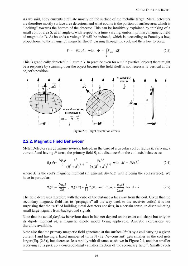
As we said, eddy currents circulate mostly on the surface of the metallic target. Metal detectorsare therefore mostly surface area detectors, and what counts is the portion of surface area which is“looking” towards the bottom of the detector. This can be intuitively explained by thinking of asmall coil of area S, at an angle α with respect to a time varying, uniform primary magnetic fieldof magnitude B. At its ends a voltage V will be induced, which is, according to Faraday’s law,proportional to the change of magnetic flux Φ passing through the coil, and therefore to cosα:
(2.3)
This is graphically depicted in Figure 2.3. In practice even for α=90° (vertical object) there mightbe a response by scanning over the object because the field itself is not necessarily vertical at theobject’s position.
2.2.2. Magnetic Field BehaviourMetal Detectors are proximity sensors. Indeed, in the case of a circular coil of radius R, carrying acurrent I and having N turns, the primary field Bz at a distance d on the coil axis behaves as:
(2.4)
where M is the coil’s magnetic moment (in general: M=NIS, with S being the coil surface). Wehave in particular:
(2.5)
The field decreases therefore with the cube of the distance d far away from the coil. Given that thesecondary magnetic field has to “propagate” all the way back to the receiver coil(s) it is notsurprising that the “art” of building metal detectors consists, in a certain sense, in discriminatingsmall target signals from background signals.
Note that the actual far field behaviour does in fact not depend on the exact coil shape but only onits dipole moment M, a magnetic dipole model being applicable. Analytic expressions aretherefore available.
Note also that the primary magnetic field generated at the surface (d=0) by a coil carrying a givencurrent I and having a fixed number of turns N (i.e. NI=constant) gets smaller as the coil getslarger (Eq. (2.5)), but decreases less rapidly with distance as shown in Figure 2.4, and that smallerreceiving coils pick up a correspondingly smaller fraction of the secondary field12. Smaller coils
Figure 2.3: Target orientation effects
V Φ∂ t with ∂⁄ Φ– Bsec Sd⋅
S∫= =
FLUX Φ PASSING THROUGH S:
MAGNETIC FIELD
α
S
B
α=0° α=45° α=90°
Sd Sd
Sd
S
α
Φ B Sd⋅S∫=
BB B
Bz d( )Nµ0I
2------------ R2
R2 d2+( )3 2⁄
------------------------------=µ0M
2π R2 d2+( )3 2⁄
------------------------------------- with M NIπR2= =
Bz 0( )Nµ0I2R------------ , Bz 2R( )= 1
11------Bz 0( ) and Bz d( )µ0M
2πd3------------ for d R»≈≈
19

CHAPTER 2
provide therefore better sensitivity (at closer ranges) and spatial resolution, but do not allow to goas deep, and scan as fast, as the larger ones.
Expressions for the magnetic field of a circular and a rectangular coil are quoted in A2.2.
Finally, let us point out that these considerations are strictly speaking valid only in the static case;they retain however their validity for low frequency electromagnetic fields, as will bedemonstrated in §3.4.2.
2.2.3. Coil ConfigurationsFigure 2.5 shows some of the most frequently encountered coil configurations. Most metaldetectors for landmine detection are of the coplanar type (left); the coils are in the same plane andcan be concentric as for example in the well-known Schiebel metal detector, or shaped like a“double-D” as in the Förster Minex 2FD which will be discussed later on. Oval shapes, whichsomewhat concentrate the field towards the centre, are also proposed by a number ofmanufacturers, as well as square coils, or differential setups (see also Figure 2.6). The “4B”design achieves good pinpointing (accurate object location), at the expense of a reducedsensitivity due to a small effective area (the overlap region near the middle; the receive coil is thesmaller one in the centre). The resulting field pattern is rather complex.
The orthogonal setup is often used in combination with larger coils for deep-seeking devices(transmit vertical, receive horizontal). The coaxial setup can be more complex, with severalreceive coils for example as in the case of some MD arrays, and/or for systems targeted at UXOdetection.
12. This is rigorously valid only for a uniform magnetic field
Figure 2.4: Magnetic field behaviour with distance (in m) for coils of different sizes (NI constant; field normalized to the field of the smallest coil at d=0)
Figure 2.5: Some of the most frequently employed coil configurations (transmit-receive systems) (Adapted from [LAG79]).
0 0.05 0.1 0.15 0.2 0.25 0.3 0.35 0.40
0.1
0.2
0.3
0.4
0.5
0.6
0.7
0.8
0.9
1 Magnetic field on the axis of two coils with radii 10cm and 20cm and same current
o: R=10 cm
+: R=20 cm
o: R=10 cm
+: R=20 cm
o: R=10 cm
+: R=20 cm
o: R=10 cm
+: R=20 cm
o: R=10 cm
+: R=20 cm
o: R=10 cm
+: R=20 cm
COPLANAR COAXIAL ORTHOGONAL
“2D” “4B”
20

METAL DETECTOR BASICS
Differential (receive) setups are also used by several manufacturers. The corresponding signalsare typically left-right symmetric and show a sharp transition, instead of a maximum, whenpassing over the object (see Figure 2.6); this setup eases pinpointing (localization of the object’scentre), helps in background suppression and enhances the separation power (localizing nearbyobjects). On the other hand mechanical tolerances are stricter, and sensitivity is probablysomewhat decreased, given that the receiving coil has been split into two, effectively halving thesensitive area.
2.2.4. Frequency Domain Metal DetectorsMetal detectors can be schematically subdivided in Frequency Domain (FD) (or ContinuousWave, CW), and Time Domain (TD) systems [ALL92, RIG99, SZY99].
Frequency Domain instruments make use of a discrete number of sinusoidal signals, very oftenjust one. Single coil and separate transmit/receive circuits are possible, as will be describedbelow.
Information on the target’s nature is contained in the amplitude and phase of the received signal,or equivalently in the real and imaginary part of the probe’s complex impedance change (∆Z), asthe detector approaches the target. Their measurement in background conditions can be used toreject part of the background signal itself, especially in areas in which the detector’s performancewould otherwise be seriously degraded, such as sea beaches (salt water is conductive) or stronglymineralized regions (containing for example bauxite, laterite, magnetite or magmatite), which canbe conductive or iron rich, as found in parts of Cambodia, Mozambique and Angola. Generallyspeaking, background rejection is more difficult in nonhomogeneous areas.
From the point of view of sensitivity there is a tendency to move towards higher operatingfrequencies, which can be probably explained by thinking of the quality factor Q improvement ofa resonant (LC) circuit, and also by the fact that the induced voltage V is proportional, accordingto Faraday’s law, to the rate of change of the magnetic flux Φ passing through the receiver coil(Eq. (2.3)). Indeed, varies as eiωt, and the same is true for Φ. Therefore13 .
On the other hand lower frequencies penetrate better, appear to be less affected by groundmineralisation and the skin effect in metal is reduced, so that a comprise solution has to be foundas usual. In the Förster Minex 2FD system an interesting strategy has been adopted, whichconsists in employing one frequency (2.4 kHz) towards the lower bound and one (19.2 kHz)towards the upper bound of the frequency range of interest. Other characteristics of higher and
Figure 2.6: Differential response vs. standard response (qualitatively) for a linear scan
13. We are simplifying here, in reality obviously depends on ω too.
SCANNING SETUP (top view) DIFFERENTIAL
RESPONSE
V (amplitude)
x xx=0
metal detector scanning line
object centre
V (amplitude)
object centre
“STANDARD” RESPONSE
x
Bsec V ωeiωt∝
Bsec
21

CHAPTER 2
lower operating frequencies will be discussed when looking at the response predicted by thetheoretical models (Chapter 3).
As an example of Frequency Domain detectors we can quote the Förster Minex 2FD, quite a fewmodels from the Ebinger line and most treasure hunting devices. Frequency Domain systemshave often been the choice for mine detection because they seem to work well especially for verysmall and close objects, except where ground conditions are severe and request the use of pulsedsystems. The possibility of using an array of frequency domain detectors is somewhatcomplicated by interference effects between neighbouring systems.
We will now discuss different ways of implementing Frequency Domain metal detectors.
2.2.4.1. Single Coil Frequency Domain Metal Detectors
A single coil can be used, whereby there are basically two ways of working.
In a first scheme the coil’s change in impedance ∆Z is detected by measuring for example thedamping of a (fixed frequency) resonant circuit, as shown schematically in the upper half ofFigure 2.7. In this simplified transformer model the coil acts as the primary winding of atransformer, the object as a “single turn” secondary winding (NS=1), representing the load on thetransformer. In practice one could measure the amplitude and/or phase of the voltage changeacross the primary coil (VP=IPZP), assuming a constant current IP.
When approaching a metallic object there would be a decrease in the probe’s impedance. Forferromagnetic objects the magnetic flux would however be strengthened14 and ∆Z increases.
In a second scheme the change in self-inductance of a single coil is measured by looking at thefrequency shift ∆fres of an oscillator in which the coil acts as the inductive element (with forexample for an LC oscillating circuit). One of the simplest methods is the BeatFrequency Oscillator (BFO), which was one of the earliest types of metal detectors and is stillused in some simple applications, such as for traffic light controls via a loop buried under thesurface. A schematic BFO implementation, which directly produces an audio signal, is shown inFigure 2.8. No ground balancing was possible with BFO systems.
Other implementations based on the modifications of the properties of a resonant circuit are alsoproposed by some manufacturers.
Figure 2.7: Simplified transformer model of a metal detector in presence of test material (buried object)
14. We can think for example of a coil whose inductance L will increase introducing into it a ferromagnetic core.
PROBE(PRIMARY COIL)
OBJECT(SECONDARY COIL)
RS
LS
LP
ISIP
RP
VP
IASECONDARY
RECEIVE COIL V
fres 1 LC( )⁄=
22

METAL DETECTOR BASICS
2.2.4.2. Frequency Domain Metal Detectors with Separate Transmit/Receive Cir-cuits
Most modern Frequency Domain metal detectors do in fact use separate transmit/receive circuitsand operate in the VLF region of the spectrum, typically between a few kHz and a few tens ofkHz (say 1-50 kHz). If we denote the voltage in the transmitter coil with V1 and in the receivercoil with V2, and M12 is the mutual inductance between the two coils, then we have that(operating at a single frequency ω):
(2.6)
with M12 = M21 (reciprocity theorem). Any change in the voltage V2 induced in the receiver coilscaused by the presence of metallic or magnetic objects can therefore be interpreted as a (usuallysmall) change in the mutual inductance M12 between the transmit and receive coil(s)15 (see againFigure 2.7). In fact, for this type of detectors the coils are often arranged to have as low a mutualinductance as possible when no object is present (i.e. minimize direct coupling of transmitted andreceived field), in order to enhance the contrast between the situation with presence and withabsence of signal. In such a setup the position of the coils can therefore be critical, for instance inpresence of large temperature gradients and/or of mechanical stress (coil flexing) which caninfluence the coil coupling.
In the case of single frequency FD instruments the secondary (or received) signal:
(2.7)
will vary sinusoidally as a function of time at the angular frequency ω of the transmitted signal,but in general phase shifted (i.e. time delayed) by ϕ with respect to the latter (for details see[VUI94]). The received signal can also be written as:
(2.8)
The first quantity, VR, is the component of the received signal in phase with the transmitted one(“in-phase” or resistive component), the second, VX, is the component of the received signaldephased by 90 degrees with respect to the transmitted signal (“quadrature-phase” or reactivecomponent); both representations are clearly equivalent.
It is therefore customary to represent the received signal Vsec as the complex quantity:
(2.9)
Figure 2.8: The Beat Frequency Oscillator (a type of single coil Frequency Domain MD) (Adapted from [GAR95])
15. Metal detectors of this type are also called Induction-Balance systems.
REFERENCEOSCILLATOR
SEARCHOSCILLATOR
MIXERAMPLIFIER
AUDIOOUTPUT
DATASTORAGE
SEARCH Freq.--REFERENCE Freq.=
AUDIO Frequency
REFERENCE Freq.
SEARCH Freq.
TUNER
Capacitance “C”
SEARCHCOIL(ANTENNA)
Inductance “L”
V1 I1eiωt and V2 = i– ωM12I1eiωt=
Vsec t( ) Asec ωt ϕ+( )sin=
Vsec t( ) Asec ωt ϕ+( )sin VR ωtsin VX ωcos t where VR+ Asec ϕcos and VX Asec ϕsin= = = =
Vsec VR iVX , i= 1–+=
23

CHAPTER 2
bidimensionally in a complex plane (or impedance plane) as a point of coordinates Vsec=(VR,VX),as schematically shown in Figure 2.9.
Note that the separation in in-phase and quadrature-phase component, which can be achievedelectronically for example by means of a synchronous demodulator16, requires a quite precisecontrol of the reference phase. For example, the accuracy of the reference phase regulation of theFörster Minex detector is of about 0.01° (about 0.17 mrad), necessary in particular to keep trackof tiny variations in the target output signals (especially when their difference is used fordetection, as we will see later) compared with often much larger background signal levels. Inaddition the reference phase regulation needs to be continuous in order to provide sufficient(thermal) stability and counteract drifts.
The amplitude Asec, and often the phase shift ϕ too (or equivalently VR and VX), will in fact varywhen the detector and the target object are moved with respect to each other, containinginformation on the target’s nature:
(2.10)
These are the quantities we are interested in and we will not be surprised by seeing later on thepoint corresponding to Vsec=(VR,VX) move in the complex plane along characteristic lines as thedetector or the target are displaced.
2.2.5. Time Domain Metal DetectorsTime Domain, or “pulse”, instruments work by passing pulses of current through a coil (typicalrepetition rate of the order of 1 kHz), taking care to minimise the current switch-off time (a fewµsec). Eddy currents are thus induced in nearby conductive objects; the exponential decay of thecorresponding secondary magnetic field, which is slower than the primary one, is observed withtime. A Time Domain metal detector measures in other words how quickly the momentarilygenerated magnetic field breaks down, which happens to be slower in presence of metal[ALL92].
Figure 2.9: Representation of the received signal as phase vector in the complex (impedance) plane
16. By sampling, for example, the sinusoidal signal at two positions 90° apart on the waveform.
VR=Asec cosϕ
VX=Asec sinϕ
RESISTIVE Component (IN-PHASE)
REACTIVE Component (QUADRATURE-PHASE)
Vsec = VR + i VX
ϕ
Vprim(t)
t
V(t)
Vsec(t)
A sec
Asec
ϕ
Transmitted and Received signals as a function of time
Complex (Impedance) Plane representation
tanϕ= VX/VR
Asec Asec t( ) , ϕ ϕ t( ) or equivalently VR VR t( ) , VX VX t( )= = = =
24

METAL DETECTOR BASICS
A practical example, referring to the Protovale pulse induction sensor for rebar location, is shownin Figure 2.10. The current in the coil starts up fairly gently (a), and is then turned off very rapidlyat the end of the pulse (a few µsec); this induces a very large voltage spike (“back e.m.f.”) (b).The cycle is repeated after about 1 msec. The eddy currents induced in a conductive target try torecreate the field that has just disappeared, and also decade graciously away (c). These eddycurrents generate a secondary magnetic field that induces a (small) voltage in the coil head, whichdecays at the same rate (actually as its time derivative) (d). The signal is sampled only after ashort delay, which ensures that the switch-off transient is over (e) [ALL92].
The eddy current decay time constant itself, some tens (short) to hundred µsec, depends(predominantly) on the target’s conductivity, permeability and size. Low conductivitybackground and nuisance items, such as sea water and thin foils for example, have a very shortdecay time. A pulse detector, which is tuned to sample only a specific portion of the receivedsignal, can therefore be “easily” made insensitive to them by an appropriate choice of the delay(some tens of µsec17) between switch-off and sample. A similar argument applies to purelymagnetic but non-conductive targets, which are magnetised by the transmit pulse but demagnetisejust as promptly after switch-off. On the other hand it was true until a few years ago that overallsensitivity is reduced in comparison with Frequency Domain detectors, and there can be problemsin finding low conductivity metallic objects such as those made of stainless steel. Figure 2.11summarizes the situation and stresses the difference between the “good” and the “poor”conductor case.
Figure 2.10: Typical pulse induction detector timing (Source: [ALL92])
17. [ROW] quotes 20 µsec, ideally, and realistically 30 to 40 µsec. Improved systems tend however to sample theentire waveform and/or start at earlier sampling times, as in [NEL01].
25

CHAPTER 2
Given that the transmit and receive phase are temporally separated – the received waveform isusually18 sampled during the time in which the transmitter is off – pulse detectors can use one andthe same coil for transmitting and receiving; the decoupling of the two phases also allows to workwith high power, and therefore in practice to go deeper (increased sensitivity due to higher fieldstrength). Power consumption might obviously become an issue, and the presence of a largeinductance (due for instance to a large number of turns and/or a large area of the transmitter coil)can cause switch-off problems.
Pulse systems are the detector of choice when it comes to working in salt water or stronglymineralised soils. They are however increasingly often challenging Frequency Domain systems,and not only where conditions are severe.
Time Domain systems are inherently broadband and sample therefore a larger portion of the VLFelectromagnetic spectrum. This information is however often not used directly, e.g. when thereceived signal is sampled only in a few points, or when its integral over a time window is used.
The interested reader will find a more detailed description of the different stages of the pulseresponse in [KAC98] and in general in the geophysical literature dealing with Time Domainsystems. Detailed time-decay data is shown for a variety of mines in [NEL01], which does alsotake into account soil effects, in particular on the response of minimum-metal mines.
Figure 2.11: Decay of the induced pulse in the no metal, good and poor conductor case (Source: Protovale)
18. Recording before the transmission phase is finished is in principle also possible.
26

METAL DETECTOR BASICS
2.3. Modern Tools
We will describe in this section present-day commercial systems, which are the result of manyyears’ efforts in increasing sensitivity and autonomy, and mastering background rejection andergonomics. The interested reader can look as a complement at the [SIG02] patent study, inparticular at the reference patents mentioned therein, of which we have incorporated here themost interesting elements.
2.3.1. Background SignalAs already hinted at in Figure 2.2, the target signal is accompanied by an omnipresentbackground signal. The latter is made up of contributions due to electromagnetic (EM)background (e.g. due to power lines or other forms of interference), to drift effects (e.g. due tothermal and/or mechanical variations) and to the soil signal itself. It should be possible to mitigatethe first two effects by a careful design of the hardware (coils, electronics) and of the signalprocessing (e.g. bandpass filtering). A differential setup should also be helpful.
We already discussed in §2.2.4 the importance of the soil signal itself, in particular in areas suchas sea beaches or strongly mineralized regions, which can be conductive or iron rich [MIL96](see also Table 3.3), as found in parts of Cambodia19, Mozambique and Angola for example. Aniron rich ground would result in a reactive component, a conductive ground in a resistive signal,which seems to be the prevalent condition in most parts of the world (with the notable exceptionof Australia).
The soil’s conductivity is indeed small compared to that of metals, but is distributed over a muchlarger volume. The resulting signal, Vsoil, can therefore be far from negligible. In such regions thedetector’s performance can be seriously degraded, especially when looking for small signals,resulting from small and/or deep objects, which can be completely masked by the ground signal.In reality, therefore (all quantities being complex):
Vsec = Vsoil + Vtarget (2.11)
In addition the magnetic susceptibility of certain soils can vary with frequency (or time) [DAS98,and refs. [10]-[20] therein mentioned], as will be discussed in Chapter 4.
In these cases some form of background rejection is essential and often relies on measuring theground signal when no metallic object is present, to then “follow” and suppress it as well aspossible. One “classical” way of implementing this in a frequency domain system with separatedtransmit/receive circuits consists in measuring the phase shift due to the ground signal alone, andproviding the received signal relative to it by means of a synchronous demodulator, as depicted inFigure 2.12.
Generally speaking, background rejection, also called “ground balancing”, is more difficult innonhomogeneous areas. Metal detectors can perform the ground balancing function automaticallyor manually, for example via a multiturn knob in FD systems, the latter option being preferred byexperts when a high degree of precision and total control of the instrument is required. Groundbalancing can in fact be extremely delicate, given that situations where one component is muchlarger than the other, up to a ratio of 1000:1 corresponding to an angle of 0.057 degrees in thephase plane, are not infrequent ([ROW] mentions “a resolution of better than 500 to 1”).Automatic ground balancing is usually preferred in systems for humanitarian demining.Sensitivity will nevertheless usually be reduced, partly because the magnetic field penetrates lesswell in the ground, and partly due to possible problems with localized soil inhomogeneities suchas voids, roots, or “hot rocks” (magnetic rocks), which would cause too many “false alarms”.
19. Mineralised (lateritic) soil was estimated to be present in 40% of the minefields in Cambodia [DAS98].
27
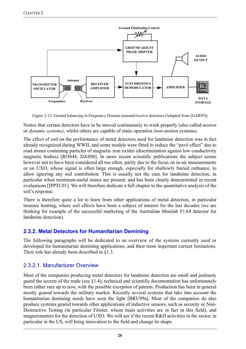
CHAPTER 2
Notice that certain detectors have to be moved continuously to work properly (also called motionor dynamic systems), whilst others are capable of static operation (non-motion systems).
The effect of soil on the performance of metal detectors used for landmine detection was in factalready recognized during WWII, and some models were fitted to reduce the “pavé effect” due toroad stones containing particles of magnetic iron oxides (discrimination against low conductivitymagnetic bodies) [ROS48, DAS98]. In more recent scientific publications the subject seemshowever not to have been considered all too often, partly due to the focus on in-air measurementsor on UXO, whose signal is often large enough, especially for shallowly buried ordnance, toallow ignoring any soil contribution. This is usually not the case for landmine detection, inparticular when minimum-metal mines are present, and has been clearly demonstrated in recentevaluations [IPPTC01]. We will therefore dedicate a full chapter to the quantitative analysis of thesoil’s response.
There is therefore quite a lot to learn from other applications of metal detection, in particulartreasure hunting, where soil effects have been a subject of interest for the last decades (we arethinking for example of the successful marketing of the Australian Minelab F1A4 detector forlandmine detection).
2.3.2. Metal Detectors for Humanitarian DeminingThe following paragraphs will be dedicated to an overview of the systems currently used ordeveloped for humanitarian demining applications, and their most important current limitations.Their role has already been described in §1.3.
2.3.2.1. Manufacturer Overview
Most of the companies producing metal detectors for landmine detection are small and jealouslyguard the secrets of the trade (see §1.4); technical and scientific documentation has unfortunatelybeen rather rare up to now, with the possible exception of patents. Production has been in generalmostly geared towards the military market. Recently several systems that take into account thehumanitarian demining needs have seen the light [BRU99a]. Most of the companies do alsoproduce systems geared towards other applications of inductive sensors, such as security or Non-Destructive Testing (in particular Förster, whose main activities are in fact in this field), andmagnetometers for the detection of UXO. We will see if the recent R&D activities in the sector, inparticular in the US, will bring innovation to the field and change its shape.
Figure 2.12: Ground balancing in Frequency Domain transmit/receive detectors (Adapted from [GAR95])
Ground Eliminating Control
AMPLIFIER
AUDIOOUTPUT
DATASTORAGE
Antenna
ReceiverTransmitter
SYNCHRONOUS DEMODULATOR
GROUND ADJUSTPHASE SHIFTER
TRANSMITTEROSCILLATOR
RECEIVER AMPLIFIER
28

METAL DETECTOR BASICS
European metal detector manufacturers are well established at international level and includeEbinger, Förster and Vallon in Germany, Schiebel in Austria, Guartel in the UK and CEIA inItaly. The other major international player is Minelab (Australia), which has entered the market afew years ago.
The total installed base in humanitarian demining is probably in the 10000 to 20000 units range,counting slightly less than one metal detector per deminer. The corresponding figure for themilitary market might be, very indicatively, double as much (the US Army has acquired fromSchiebel about this many detectors at the beginning of the ‘90s). The total number of units soldeach year for humanitarian demining does probably not exceed a few thousand, which wouldimply yearly sales in the order of a few tens of millions of Euro. This gives an idea of the marketinvolved, although the importance of related markets should not be underestimated, in particularthe detection of UXO for site remediation. Summarizing
• Mostly specialized SME (Small to Medium Enterprises). Little technical/scientific literature(Intellectual Property Rights issues!).
• Strong European position. Installed base ~ 10000-20000.• Some increase in R&D outside the traditional manufacturer area• Strong similarities between military and humanitarian demining systems
2.3.2.2. Man Portable Systems
Metal detectors for humanitarian demining are remarkable active sensors capable of detectingtiny amounts of metal, from a fraction of a gram onwards, at shallow depths. Frequency Domainsystems have often been the choice because they seem to work well especially for very small andclose objects, but they are being more and more challenged by pulse systems, and not only whereground conditions are severe. Portable systems share the following characteristics (true for mostmodels):
• Weight: less than 2 kg. Price: in the 2000-4000 Euro range.• Size: round, oval or rectangular head. In the former case the diameter is between 20 and 30 cm, to
achieve sufficient depth and a reasonable scanning surface and speed; the thickness is of about acouple of cm.
• Operating depth: shallow, i.e. from flush (even with the surface) down to about 10-15 cm forminimum-metal mines, 20-30 cm for mines with an appreciable metallic content, and about 50-70cm for large metallic objects such as UXO or metallic mines. Can reach deeper using large loopdetectors, as alternative/complement to magnetometers.
• Electrical/Mechanical: capable of working with standard cell batteries for a long time (tens ofhours), and usually simple to use. Many demining teams pay more attention to the ergonomicsrather than to the pure performances of the detector itself.
• Output: normally an audio signal, usually already the result of extensive internal data processing,from which an experienced operator can make some qualitative statement on the target type andposition/depth. When using manual methods as the primary procedure, each alarm is carefullychecked until it has been fully understood and/or its source removed.
To the best of our knowledge no current metal detector for humanitarian demining applicationsdelivers some quantitative information on the object under analysis. This is astonishing at firstview, since there are other disciplines like Non-Destructive Testing where this is the case. It canprobably be explained by the urgent priority to enhance detection performance through betterbackground rejection (i.e. reduction of the metal detector false alarm rate) and achieving highersensitivity, as well as by the need of being very precise whilst usually not having any a prioriinformation on the object under analysis. Additional comments have been provided in §1.4.
29
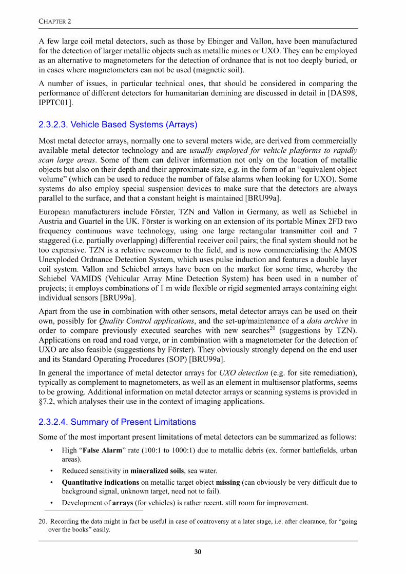
CHAPTER 2
A few large coil metal detectors, such as those by Ebinger and Vallon, have been manufacturedfor the detection of larger metallic objects such as metallic mines or UXO. They can be employedas an alternative to magnetometers for the detection of ordnance that is not too deeply buried, orin cases where magnetometers can not be used (magnetic soil).
A number of issues, in particular technical ones, that should be considered in comparing theperformance of different detectors for humanitarian demining are discussed in detail in [DAS98,IPPTC01].
2.3.2.3. Vehicle Based Systems (Arrays)
Most metal detector arrays, normally one to several meters wide, are derived from commerciallyavailable metal detector technology and are usually employed for vehicle platforms to rapidlyscan large areas. Some of them can deliver information not only on the location of metallicobjects but also on their depth and their approximate size, e.g. in the form of an “equivalent objectvolume” (which can be used to reduce the number of false alarms when looking for UXO). Somesystems do also employ special suspension devices to make sure that the detectors are alwaysparallel to the surface, and that a constant height is maintained [BRU99a].
European manufacturers include Förster, TZN and Vallon in Germany, as well as Schiebel inAustria and Guartel in the UK. Förster is working on an extension of its portable Minex 2FD twofrequency continuous wave technology, using one large rectangular transmitter coil and 7staggered (i.e. partially overlapping) differential receiver coil pairs; the final system should not betoo expensive. TZN is a relative newcomer to the field, and is now commercialising the AMOSUnexploded Ordnance Detection System, which uses pulse induction and features a double layercoil system. Vallon and Schiebel arrays have been on the market for some time, whereby theSchiebel VAMIDS (Vehicular Array Mine Detection System) has been used in a number ofprojects; it employs combinations of 1 m wide flexible or rigid segmented arrays containing eightindividual sensors [BRU99a].
Apart from the use in combination with other sensors, metal detector arrays can be used on theirown, possibly for Quality Control applications, and the set-up/maintenance of a data archive inorder to compare previously executed searches with new searches20 (suggestions by TZN).Applications on road and road verge, or in combination with a magnetometer for the detection ofUXO are also feasible (suggestions by Förster). They obviously strongly depend on the end userand its Standard Operating Procedures (SOP) [BRU99a].
In general the importance of metal detector arrays for UXO detection (e.g. for site remediation),typically as complement to magnetometers, as well as an element in multisensor platforms, seemsto be growing. Additional information on metal detector arrays or scanning systems is provided in§7.2, which analyses their use in the context of imaging applications.
2.3.2.4. Summary of Present LimitationsSome of the most important present limitations of metal detectors can be summarized as follows:
• High “False Alarm” rate (100:1 to 1000:1) due to metallic debris (ex. former battlefields, urbanareas).
• Reduced sensitivity in mineralized soils, sea water.• Quantitative indications on metallic target object missing (can obviously be very difficult due to
background signal, unknown target, need not to fail).• Development of arrays (for vehicles) is rather recent, still room for improvement.
20. Recording the data might in fact be useful in case of controversy at a later stage, i.e. after clearance, for “goingover the books” easily.
30

METAL DETECTOR BASICS
2.3.3. Metal Detectors for HobbyistsMetal detectors designed for hobbyists are mostly simpler and less expensive than theirhumanitarian demining counterparts, but make use in some cases of interesting innovations andare supposed to possess some target classification capabilities. As such they deserve a closer look.
We will comment in the following mostly on FD systems. Some additional information can befound for example in [ROW], in the [SIG02] patent study, and to a lesser extent for what concernsscientific details in publications which are more application oriented and intended for a wideaudience such as [GAR95, LAG79]. An exception was [LeG69], which started from basicelectronics and managed to achieve, without using a single (explicit) formula, a remarkable andin-depth review of the physics/technology of the subject.
2.3.3.1. VLF Transmitter/Receiver (Induction Balance) Systems
Although Frequency Domain metal detectors for hobbyists, e.g. for “treasure hunting” might notmeet some of the standards of humanitarian demining in terms of ease of use, robustness, orreproducibility, it is true that they have incorporated target classification capabilities(“discrimination”) for quite some time. This discrimination is basically a sorting of metallicobjects based primarily on their phase angle response21 (the signal strength can also play a role).
Indeed, as we will also see in the theoretical analysis of a Simple Circuit Model (§3.1), the largestphase shift will occur for metal objects which are primarily inductive; large, thick objects madefrom excellent conductors like gold, silver, and copper. Smaller phase shifts are typical forobjects which are primarily resistive; smaller, thinner objects, or those composed of lessconductive materials. Purely ferromagnetic materials, including most soils and sands, are on theother hand reported as having little or no phase shift [ROW].
Target discrimination also takes advantage from the fact that in some instances the target objectsare known a priori, as is for example the case with coins (all US coinage is apparentlyconsistently minted). A calibration is therefore possible and pattern of responses can be stored ina small database for the most advanced (microprocessor based) detectors, preanalysing the soiland all detected target responses (phase shift and signal strength). In this case the object’sapproximate depth can also be indicated once it has been identified, using the measured signalstrength and knowing the detector’s parameters (coil size, transmit current). Iron targets arecharacterised as “orientation sensitive”, as we will confirm in Chapters 5 and 6, and the measuredphase may change dramatically when moving the coil over them [ROW].
The discrimination can consist in a simple threshold on the phase shift, or “notch discrimination”in which only targets within a given phase angle range are considered. The metal detector mayprovide a numeric read-out, meter indication or another type of visual display. An example isprovided in Figure 2.13: a number based on the measured phase is displayed on the horizontalaxis, the signal strength on the vertical axis. This type of display is apparently very useful indistinguishing trash from more valuable objects. The distinction between ferrous and non-ferrousobjects is evident, as well as the sorting of the latter into metal type (nickel and aluminium, USpennies and quarters, etc.).
Some practical problems to such a classification approach have been reported with some objecttypes such as aluminium foil, or pull-tabs, possibly bent or broken, because of their large surfaceto volume ratio. How good discrimination is in general also remains an open question, and onecan expect that target identification will be more problematic with targets delivering weakresponses, and/or being deep22. Herein lies the question to be answered when thinking oftransposing it to humanitarian demining applications.
21. White’s Electronics, Private Communication, 1997.
31

CHAPTER 2
The possibility also exists that a detector, passing over (or near) a rejected target and then over agood one, will not detect (i.e. mask) the latter [CON96].
2.3.3.2. Ground Balance
As already indicated, in any practical scheme it will be of fundamental importance to separate thesignal due to the target from the soil signal itself, which can be much stronger. What can beexploited is the fact that the phase shift due to the ground tends to remain fairly constant over alimited area [ROW], whereas the target response changes quickly when moving over it. Someground balancing schemes have already been described in §2.3.1, and additional information canbe found in [ROW] and [SIG02] in particular.
2.3.3.3. Advanced Systems
The use of multiple frequencies should enhance target discrimination capabilities, as well asease background rejection. A number of manufacturers are proposing multifrequency systems,e.g. Minelab (Australia) using a technique termed Broad Band Spectrum (17 separate frequenciesfrom 1.5 kHz to 22.5 kHz transmitted together), and probably White’s (US) with its SpectrumXLT. Concerning time domain systems, the use of special pulse sequences has been adopted tocope in particular with severe ground conditions, e.g. again by Minelab with a technique termedMulti-Period Sensing. More information is available from the manufacturers’ Websites andsometimes from their patents as well (see for instance the Candy/Minelab patents in [SIG02]).
22. The response of deeper targets will change more slowly than the one of shallow targets, and thus be more difficultto separate from the soil response.
Figure 2.13: White’s Electronics “SignaGraph”™ display [ROW]
32

METAL DETECTOR BASICS
2.4. Advanced Developments
Although the integration of mine detection dogs and mechanical system into humanitariandemining activities has considerably progressed in the last years, metal detectors do still play aconsiderable role and are present in nearly every multi-sensor system being researched (§1.3).
There are however a number of improvements proposed and studied for the metal detector itself,whether used together with other sensors or standalone. Apart from a further amelioration of thebackground rejection, we have already seen that the measured signal is rich in information(Figure 2.2):
Vsec = V(σ,µ,R,d,...) (2.12)
The possibility of delivering quantitative information on the target under analysis is thereforeactively studied, such as:
• Depth, using overlapping coils or signal profile study (scanning on a line over the object);• “Size”, possibly with a rough estimate (small (=debris?) vs. large);• Object Type (could be useful in situations where there are only a few targets in a given area);• Object Shape (not easy to reach sufficient resolution; useful for larger objects?).
The practical usefulness of this approach is however still debated in the end user community.
We are in fact attempting to solve one or more facets of the inverse electromagnetic inductionproblem (see A1.1), whose aim is to determine the position (in particular the depth), shape, sizeand material parameters (conductivity σ, permeability µ) of a hidden object. In the general casethis turns out to be a very difficult problem, and we are not aware of any general solution whichdoes not rely on some a priori information or assumption. In addition it is in general much easierto detect an anomaly than to classify it (i.e. saying that “there is something” rather than saying“there is an object of a given type”), and classification results get usually worse with decreasingsignal to noise ratio. Background effects and implementation constraints do also complicate theproblem’s solution.
We will therefore now review some different aspects of inverse electromagnetic inductionproblems, having in mind as far as possible practical limitations and applications. Indeed, anumber of parameters will also strongly determine if the system will ever be fielded, e.g.importance of the target application (i.e. humanitarian demining problem specificity and realequipment price/performance enhancement), equipment cost, size, complexity, penetration depth,simple and/or user friendly man machine interface (MMI), etc. [BRO98]. The risk of R&D is, asColin King once put it, to devise systems which “work best where they are least useful”[BRU99a, KIN96]. Emphasis will be put in this section on qualitative aspects, quantitative oneswill be the subject of the next chapter.
2.4.1. Object Characterisation (Object Type/Size)Information on the target’s nature and/or position is contained in the frequency or time responsewhen above it, in the spatial dependency of the response when scanning along a line across it oron a horizontal surface for example, or obviously by combinations thereof.
In the general case an object’s response depends on many parameters (Figure 2.2), and thescenario is complicated by additional factors: i) some parameters are lumped together into asingle response parameter (§3.3), ii) the response can be orientation dependent, iii) the soilresponse has to be added as well, iv) the response is strongly dependent on the target’spermeability, v) objects can be composite, etc.
33

CHAPTER 2
It is therefore usually necessary to make some assumptions to simplify the problem and try to“disentangle” the dependencies on the target’s parameters, at least for those assumed to be ofinterest for the given scenario(s). If the objects are known to be “small” it makes sense to use adipole model, if they are known to be mostly ferromagnetic one can assume that their magneticpermeability is high, if one is looking for UXO most targets are likely to be elongated, etc.
As briefly discussed in A1.1, there are two general techniques that may be used to estimate thetarget parameters from measurements, namely “model fitting” and “pattern recognition”.
• In the first approach – model fitting – one has to devise a mathematical model to describe thesecondary (induced) fields as a function of the source parameters, which are then recovered by aninversion procedure. When using for example an induced dipole model (§3.6.1) one recovers thetarget’s magnetic polarizability tensor. This quantity fully characterizes in principle the target’sEM properties, but has usually to be further evaluated. A partial evaluation might already provideinformation on the target’s symmetry [MER00], which represents in a number of situations a goodindicator.Other models can be directly expressed as a function of the target’s physical and electromagneticparameters (σ,µ), or indirectly via derived quantities such as L/R in a simple circuit model (§3.1),the position of the object’s pole(s) in the frequency domain (or equivalently its time decayconstant(s) in the time domain) when thinking in terms of natural modes (§3.6.3), or its responseparameter discussed above in the general case.A combination of different successive approaches to recover the parameters which are lumpedtogether (σ,µ and sphere radius for example) is also possible in principle. The target’spermeability can for instance be recovered using a magnetometer or a quite low frequency,followed by an estimate of the depth (from a fit of the spatial field dependency for example)which allows to estimate the object’s volume knowing the signal amplitude (in an induced dipolemodel), and therefore its radius. At this point one can calculate the conductivity from themeasured response parameter at a given frequency.Variations of simple models to cope with background signals have also been devised ([PAT99]and other similar patents [SIG02]).Model fitting is obviously limited by there being an applicable model, or conversely by howapplicable/realistic the chosen model is. At the end of the day the information having beenrecovered might or might not be sufficient for the given task – in general some knowledge of thetargets being sought is necessary as well.
• In the second approach – pattern recognition – characteristics of a set of EM data from anunknown object are compared with that from a known one, to determine if the two objects are thesame. Pattern recognition is in a certain sense used by the deminers themselves, when theyinterpret the detector’s audio signal and try to assess an object’s depth and size by comparing itwith what they are familiar.Some form of data reduction or compression (“feature extraction”) might be necessary to makepattern recognition feasible. Ideal features have a high resolution capability, that is are capable ofwell separating objects belonging to different classes. It will however be sometimes necessary totrade resolution power for applicability and rely on less discriminating features. In some caseslarge libraries of feature vectors can be required. Also, the problem becomes usually less tractableas the number of possible object shapes and sizes increases.An example of a pattern recognition approach is EM induction spectroscopy (§3.6.2), whichconsists in measuring a target’s induction response a several frequencies and comparing it to a setof known responses.Possible problems with the pattern recognition approach are represented by the stability of thechosen features, and the presence of unknown targets.
34
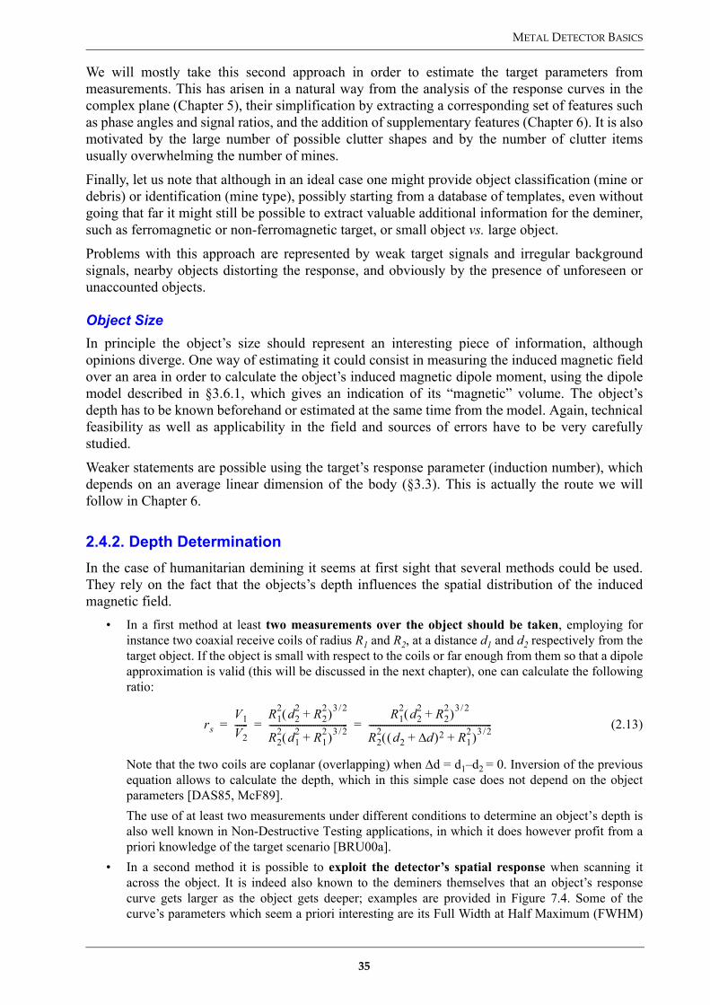
METAL DETECTOR BASICS
We will mostly take this second approach in order to estimate the target parameters frommeasurements. This has arisen in a natural way from the analysis of the response curves in thecomplex plane (Chapter 5), their simplification by extracting a corresponding set of features suchas phase angles and signal ratios, and the addition of supplementary features (Chapter 6). It is alsomotivated by the large number of possible clutter shapes and by the number of clutter itemsusually overwhelming the number of mines.
Finally, let us note that although in an ideal case one might provide object classification (mine ordebris) or identification (mine type), possibly starting from a database of templates, even withoutgoing that far it might still be possible to extract valuable additional information for the deminer,such as ferromagnetic or non-ferromagnetic target, or small object vs. large object.
Problems with this approach are represented by weak target signals and irregular backgroundsignals, nearby objects distorting the response, and obviously by the presence of unforeseen orunaccounted objects.
Object SizeIn principle the object’s size should represent an interesting piece of information, althoughopinions diverge. One way of estimating it could consist in measuring the induced magnetic fieldover an area in order to calculate the object’s induced magnetic dipole moment, using the dipolemodel described in §3.6.1, which gives an indication of its “magnetic” volume. The object’sdepth has to be known beforehand or estimated at the same time from the model. Again, technicalfeasibility as well as applicability in the field and sources of errors have to be very carefullystudied.
Weaker statements are possible using the target’s response parameter (induction number), whichdepends on an average linear dimension of the body (§3.3). This is actually the route we willfollow in Chapter 6.
2.4.2. Depth DeterminationIn the case of humanitarian demining it seems at first sight that several methods could be used.They rely on the fact that the objects’s depth influences the spatial distribution of the inducedmagnetic field.
• In a first method at least two measurements over the object should be taken, employing forinstance two coaxial receive coils of radius R1 and R2, at a distance d1 and d2 respectively from thetarget object. If the object is small with respect to the coils or far enough from them so that a dipoleapproximation is valid (this will be discussed in the next chapter), one can calculate the followingratio:
(2.13)
Note that the two coils are coplanar (overlapping) when ∆d = d1–d2 = 0. Inversion of the previousequation allows to calculate the depth, which in this simple case does not depend on the objectparameters [DAS85, McF89].The use of at least two measurements under different conditions to determine an object’s depth isalso well known in Non-Destructive Testing applications, in which it does however profit from apriori knowledge of the target scenario [BRU00a].
• In a second method it is possible to exploit the detector’s spatial response when scanning itacross the object. It is indeed also known to the deminers themselves that an object’s responsecurve gets larger as the object gets deeper; examples are provided in Figure 7.4. Some of thecurve’s parameters which seem a priori interesting are its Full Width at Half Maximum (FWHM)
rsV1V2------
R12 d2
2 R22+( )3 2/
R22 d1
2 R12+( )3 2/------------------------------------
R12 d2
2 R22+( )3 2/
R22 d2 d∆+( )2 R1
2+( )3 2/--------------------------------------------------------= = =
35

CHAPTER 2
and the slope’s behaviour, in particular the tails. It might also be possible to find a suitable analyticform for the curve’s profile and use it to fit the experimental data, or match against a library ofknown responses [DAS90, THO98].Two different objects at the same depth do however not necessarily produce identical spatialresponses. In addition it is necessary to avoid excessive sensor height fluctuations.
• In a third method data is collected in a horizontal plane across the target and an induced dipolemodel is used to extract the values of the object’s permeability tensor (see §3.6.1 for details). Thetarget depth is one of the problem’s parameters and can therefore be one of the results of theinversion as well.
2.4.3. Shape DeterminationA complementary approach consists in providing information on the object’s size and shape,which could be useful in discriminating in certain circumstances mines and/or UXO from clutter.“Conventional” metal detectors can indeed be used to generate images of buried metallic objectswith varying levels of resolution. This will be the subject of Chapter 7.
2.4.4. Current Research ActivitiesSome improvements should be possible using or slightly modifying existing sensors, e.g.multifrequency or advanced pulse induction detectors. Others may require more radicalapproaches, such as:
• New types of sensors: It has been suggested to study sensors other than the ordinary coilscurrently used in metal detectors, e.g. giant magnetoresistive elements, or miniature fluxgateelements. They are expected to be broadband and provide better spatial accuracy; the constructionof linear or bidimensional arrays should also be possible, delivering some kind of localised“image” of the soil metallic/magnetic contents (see §7.2 for details). On the other hand theiroverall sensitivity is likely to be smaller, which might very well discourage their use for certainapplications (their use might be envisaged for the detection of UXO or mines with a relevant metalcontent, but not for minimum-metal mines).Research on an advanced Active/Passive Magnetic Gradiometer combining sensitive magneticsensors with advanced techniques of applied field rejection has also been reported [CZI96].
• New sensor geometries (e.g. different coil arrangements): Another direction of research couldconsist in the study of “improved” magnetic field shapes, more compact than what is obtained withordinary circular or rectangular coils, or featuring some other special structure (e.g. spatiallyperiodic, see the description of the Meandering Winding Magnetometer in §7.2).
• More complete field measurements: Full measurement of the induced magnetic field vector forexample, possibly using a rotating primary magnetic field which would allow to “illuminate” theobject from different directions without actually having to move the detector (the soil responsewould probably change as well). A problem might be in the sensitivity to small pieces, if thedistance from the coils to the ground has to be increased in order to accomodate a coil geometrycapable of generating the required field geometry.
• Combine with some form of “cavity detector”: The idea of using metal detectors to actually locatenon-conducting targets, or more generally “cavities” in the soil, is not new, as a (large) non-conducting target does indeed alter locally the natural ground conductivity and/or permeability,and has led to the patent described in [MIL96]. A similar approach is detailed in [FOR00] using athree or four frequency system, as extension of the existing Minex detector.The possibility of detecting minimum-metal mines due to the void they create in some types ofelectrically lossy soils has also been clearly documented and discussed in [NEL01] using a timedomain (pulse) detector; the void effects manifest themselves in the early time region, belowabout 10 µsec. Numerical frequency domain results of the effect of a void in a conductingbackground, represented as a lossless dielectric object situated in a lossy dielectric medium, are
36

METAL DETECTOR BASICS
reported in [YU00]; the expected enhancement of the void’s signature with increasing soil watercontent (and therefore soil conductivity) is clearly demonstrated.A cavity detector should work best for large objects in soils with high natural conductivity(“background” signal), looking for distinct localized changes in the ground signal. A quiteinteresting combination is represented by a “cavity detector” coupled to a metal detector, inwhich only cavities containing some metal, such as minimum-metal mines, would be detected. Inthis case it would not be necessary to classify metallic targets, the fact that they are coincident ornot with a cavity would be sufficient.
• There is still some room for improvements of arrays; some of the corresponding research topicswill be detailed in Chapter 7.
2.5. Conclusions
In this chapter we have defined and introduced metal detectors and their basic principles, fromthe physics as well as from the technology point of view. We have looked in particular atFrequency Domain systems, which are the subject of choice of this work, and have introduced thevariables which characterise their response, and which will be analysed in more detail in Chapters3 and 4 (theory) as well as in Chapters 5 and 6 (experiment). The importance of soil effects hasalso been stressed; they will be the subject of Chapter 4.
The apparent lack of quantitative output from sensors used for humanitarian demining on onehand, and the end user need for more information on the other, have prompted us to identify needsand opportunities for improvements, which are related to different aspects of the solution of theinverse electromagnetic induction problem. Some of them will be tackled in the followingchapters, with the aim of providing target information which is nowadays mostly missing.
Concerning current research activities we have stressed research work on new types of sensorsand the possibility of combining metal detectors with some form of cavity detectors, therebycombining two features which are quite characteristic of most mines: the presence of some metalin an area where the soil is absent. Research into this direction will deserve a closer look in thefuture.
37

CHAPTER 2
Bibliography
[ALL92] J.C. Alldred, “The Pulse-Induction Principle”, Protovale Oxford Ltd., Abingdon, England,Technical Note T-41, November 1992. http://www.protovale.co.uk/abtpi.html (reduced onlineform). Interesting short technical note on the pulse induction principle.
[ALL97] Alldred, J.C. Bar-Sizing of Reinforcement in Concrete – Comparison of Available Methods.Proceedings of the Fourth Int. Conference on Non-Destructive Testing in Civil Engineering,University of Liverpool, UK, 8-11 Apr. 1997, ISBN 0-903132-23-0.
[BRO98] Brooks, J.; Nicoud, J.D. Applications of GPR Technology to Humanitarian DeminingOperations in Cambodia: Some Lessons Learned. Proceedings of the Third Annual Symposiumon Technology and the Mine Problem, Naval Postgraduate School, Monterey, CA, USA, 6-9Apr. 1998. Available online as ref. Brooks98a at http://diwww.epfl.ch/lami/detec/
[BRU99a]C. Bruschini, K. de Bruyn, H. Sahli, J. Cornelis, and J.-D. Nicoud, “EUDEM: The EU inHumanitarian DEMining – Final Report (Study on the State of the Art in the EU related tohumanitarian demining technology, products and practice)”, EPFL-LAMI and VUB-ETRO,Brussels, Belgium, July 1999. Available from http://www.eudem.vub.ac.be/ and http://diwww.epfl.ch/lami/detec/.
[BRU00a]C. Bruschini, “Metal detectors in civil engineering and humanitarian de-mining: overview andtests of a commercial visualising system”, INSIGHT – Non-Destructive Testing and ConditionMonitoring, vol. 42, no. 2, pp. 89-97, February 2000. Also available from http://diwww.epfl.ch/lami/detec/.
[BUN96]Bungey, H.; Millard, S.G. Testing of concrete in structures, 3rd ed. Blackie Academic &Professional, London, UK, 1996, ISBN 0-7514-0241-9.
[CHE84] R. H. Chesney, Y. Das, J. E. McFee, and M. R. Ito, “Identification of Metallic Spheroids byClassification of Their Electromagnetic Induction Response”, IEEE Trans. on Pattern Analysisand Machine Intelligence, vol. PAMI-6, no. 6, pp. 809-820, Nov. 1984.
[CON96]C. Conger, “Fisher CZ6a, Garrett GMH CXIII and White’s XLT” (comparative evaluation),1996. Online at http://www.polbox.com/p/proscan/titans.htm
[CZI96] Czipott P.V., Iwanowski M.D., “Magnetic sensor technology for detecting mines, UXO, andother concealed security threats”, in Terrorism and Counterterrorism Methods andTechnologies, Proc. SPIE No. 2933, pp. 67-76, 20-21 Nov., 1996.
[DAS85] Y. Das, J. E. McFee, and R. H. Chesney, “Determination of Depth of Shallowly Buried Objectsby Electromagnetic Induction”, IEEE Trans. on Geoscience and Remote Sensing, vol. 23, no. 1,pp. 60-66, Jan. 1985.
[DAS90] Y. Das, J. E. McFee, J. Toews, and G. C. Stuart, “Analysis of an Electromagnetic InductionDetector For Real-Time Location of Buried Objects”, IEEE Trans. on Geoscience and RemoteSensing, vol. 28, no. 3, pp. 278-288, May 1990.
[DAS98] Y. Das, and J. Toews, “Issues in Performance Evaluation of Metal Detectors”, in Proc. UXOForum 1998, 8 pp.
[FOR00] F. M. Förster, “Method and Device for Locating and Identifying Search Objects Concealed inthe Ground, Particularly Plastic Mines“, US Patent #6,097,190, 1 Aug. 2000. See also theGerman patent DE 196 48 833, 28 May 1998.
[GAR95]C. Garrett, “Totally Revised Modern Metal Detectors”, Second Ed., Ram Publishing Company,Dallas, Texas, 1995. ISBN 0-915920-75-1.
[HUG1879]D. E. Hughes, “Induction-balance and Experimental Researches therewith”, The London,Edinburgh and Dublin philosphical magazine and journal of science (Phil. Mag.), LondonTaylor & Francis 1876-1900, (Ser. 5) vol. 8, pp. 50-56, 1879.
[IPPTC01]Das, Y., Dean, J. T., Lewis, D., Roosenboom, J. H. J., and Zahaczewsky, G. (Eds.),International Pilot Project for Technology Co-operation – Final Report (A multi-nationaltechnical evaluation of performance of commercial off the shelf metal detectors in the context
38

METAL DETECTOR BASICS
of humanitarian demining), publication EUR 19719 EN, published by the EuropeanCommission, Joint Research Centre, Ispra, Italy, July 2001. Available from http://demining.jrc.it/ipptc/
[KAC98]P. J. Kaczkowski, “Pulsed Electromagnetic Induction (PEMI) for UXO Discrimination in JPGPhase IV – Preliminary Results”, in Proc. UXO Forum 1998, 9 pp.
[KAU01]A. A. Kaufman, and P. A. Eaton, The Theory of Inductive Prospecting. Amsterdam, NL:Elsevier, 2001.
[KEI97] D. A. Keiswetter, E. Novikova, I. J. Won, T. M. Hall, and D. Hanson, “Development of aMonostatic, Multifrequency Mine Detector”, in Detection and Remediation Technologies forMines and Minelike Targets II; SPIE Proceedings Vol. 3710 (Orlando, FLA, USA, April 21-24,1997, pp. 831-839).
[KIN96] King C. Mine Clearance…in the Real World. Proceedings of the Technology and the MineProblem Symposium, Naval Postgraduate School, Monterey, CA, USA, 18-21 Nov. 1996, pp.3-3/3-9.
[JPL95] Peterson J.C. (Study Team Leader) Sensor Technology Assessment for Ordnance and ExplosiveWaste Detection and Location. Jet Propulsion Laboratory, Report JPL D-11367 Rev. B,Pasadena, CA, USA, Mar. 1995.
[LAG79] R. Lagal and C. Garrett, “The complete VLF-TR Metal Detector Handbook”, Ram PublishingCompany, Dallas, Texas, 1979. ISBN 0-915920-32-8 [NOTE: probably out of print].
[LeG69] E.S. LeGaye, “Electronic Metal Detector Handbook”, Houston: Western Heritage Press, 1969[NOTE: probably out of print].
[McF89] J.E. McFee, “Electromagnetic Remote Sensing; Low Frequency Electromagnetics”, DefenceResearch Establishment Suffield, Ralston, Alberta, Canada, Suffield Special Publication No.124 (report DRES-SP-124), January 1989.
[MER00]L. Merlat, and P. Druyts, “Progress Report on the Metal Detector: Signal Processing for TargetDiscrimination and Coil’s Modelization”, Progress Report of the HUDEM Project, RoyalMilitary Academy, Brussels, Belgium, 29 Feb. 2000. Also ISL (Institut de Saint-Louis)Publication PU 322/2000, Saint-Louis, France.
[MIL96] Mills D., “Improvements to Mine Detectors”, Australian patent application No. PO1408, 1996.[NEL01] C. V. Nelson, et al., “Wide Bandwidth Time-Domain Electromagnetic Sensor for Metal Target
Classification”, IEEE Trans. on Geoscience and Remote Sensing, vol. 39, no. 6, pp. 1129-1138,June 2001.
[PAT99] W. Patzwaldt, “Method for the operation and for the evaluation of signals from an eddy currentprobe and device for performing the method“, US Patent #6,005,392, 21 Dec. 1999.
[POD82] M. Poddar, “A rectangular loop source of current on a two-layered Earth,” Geophys. Prospect.,vol. 30, no. 1, pp. 101-114, 1982.
[RIG99] L. S. Riggs, T. Barnett, L. Lowe, J. E. Mooney, and R. Weaver, “Baseline performance of theU.S. Army’s AN/PSS-12 metal detector”, in Detection and Remediation Technologies forMines and Minelike Targets IV; SPIE Proceedings Vol. 3710 (Orlando, FLA, USA, April 1999,pp. 52-63).
[ROC99] G. Rocker, “Systeme zur Detektion und Ortung von Gegenständen und Personen” (Systems forDetecting and Locating Objects and Persons) (in German), Erfinderaktivitäten 1998, DeutschesPatent- und Markenamt (German Patent Office), 1999, 10 pp.
[ROS48] B. Roston, “Development of Locators of Small Metallic Bodies buried in the Ground”, Journalof the Institution of Electrical Engineers (IEE Review), vol. 95, pp. 653-667, 1948.
[ROW] M. Rowan, and W. Lahr, “How Metal Detectors Work”, White’s Electronics. Available fromhttp://www.treasurenet.com/whites/howmetaldetectorswork.html
[SIG02] Sigrist, C., and Bruschini, C., “Metal Detectors for Humanitarian Demining: a Patent Searchand Analysis”, EUDEM2 report, May 2002. Available from http://www.eudem.vub.ac.be/
[SZY99] P. Szyngiera, “A Method of Metal Object Identification by Electromagnetic Means”, in Proc.
39

CHAPTER 2
MINE’99 (Mine Identification Novelties Euroconference) (Florence, Italy, October 1-3, 1999,pp. 155-160). Available from http://demining.jrc.it/aris/events/mine99/index.htm.
[THO98] O. Thonnard, “Détecteur de Métaux – Analyse d’un Détecteur de Métaux et Conception d’unSystème de Balayage afin de Produire des Images 2-D du Sol” (Metal Detector – Analysis of aMetal Detector and Design of a Scanning System for the Generation of 2-D Soil Images),Signal Image Centre, École Royale Militaire (Royal Military Academy), Brussels, Belgium,1998 (M.Sc. Thesis, in French).
[YU00] T. Yu, and L. Carin, “Analysis of the Electromagnetic Inductive Response of a Void in aConducting-Soil Background”, IEEE Trans. on Geoscience and Remote Sensing, vol. 38, no. 3,pp. 1320-1327, May 2000.
[VUI94] P.-L. Vuillermoz, Les courants de Foucault – Principes, mesure et contrôle, AFNOR, Paris,1994 (in French).
40

METAL DETECTOR BASICS
Appendix A2.
A2.1. Eddy Currents and the Skin EffectThroughout this paragraph we will assume that the magnetic (B) and electric (E) fields propagateinstantaneously, which is equivalent to neglecting displacement currents (§3.4.2). Thisassumption introduces a negligible error at low frequencies, or when the wavelength is larger thanthe typical dimensions under consideration (e.g. size of a measurement apparatus).
In this case we can give the following explanation for the setup of eddy currents (at least inextended conductors): an alternating magnetic field B(t), such as the one generated by aradiofrequency driven coil, will induce by Faraday’s law an oscillating electric field E(t),where23:
(A2.1)
A current of density J will therefore flow following Ohm’s law (σ is the conductivity):
(A2.2)and these currents, flowing in a conductor of (uniform) permeability µ, will in turn produce a(secondary) magnetic field according to Ampère’s law:
(A2.3)This justifies the statement that eddy currents exist because of time-varying magnetic fields andare basically governed by the law of induction (Faraday’s law). It also delivers a qualitativeexplanation for the fact that eddy currents are characterized by circulatory paths24 and are oftendepicted as closed loops circulating in planes perpendicular to the magnetic flux, as shown inFigure 2.14. More generally speaking we can say that eddy currents travel parallel to a coil’swinding and parallel to the surface.
Figure 2.14: Pictorial view of eddy currents in a conductor placed in a time-varying (homogeneous) magnetic field
Note also that eddy currents flowing at any depth in the conductor will generate magnetic fieldswhich, as a consequence of Lenz’s law, will be opposed to the primary field. The total magneticflux will therefore be reduced and the current flow will decrease for increasing depth.Alternatively one can think of the eddy currents on the surface as shielding the primary magneticfield and therefore weakening it with increasing depth. It can be shown that, for a sinusoidallyvarying induction of angular frequency ω, the eddy current density Jx behaves (in a thickconductor) as a function of the distance x from the surface in the following way:
23. The differential form of Maxwell’s equations will be used here.24. Here lies indeed the origin of the term “eddy”.
E∇× t∂∂B–=
J σE=
B∇× µJ=
B t( )
PRIMARY MAGNETIC
FIELD
EDDY CURRENT
LOOPS
SECONDARY (INDUCED) MAGNETIC
FIELD
CONDUCTOR
41

CHAPTER 2
(A2.4)
where δ is the skin depth in the given material at the frequency ω, and J0 the value at the surface.This equation contains the well known exponential decrease modulated by an oscillating term, atthe frequency ω of the primary field, its phase depending on the depth x. The last point is in factinstrumental in Non Destructive Testing to determine the depth of a defect in a sample (the defect,a crack for example, introduces a local change in the eddy current path).
A2.2. The magnetic field of a circular and a square coilEven in a case as simple as that of a circular loop a general analytical expression for themagnetic field does not exist. Elliptical integrals have to be numerically evaluated [KAU01,§2.2.3]. As an alternative one can use the following series expressions for the scalar magneticpotential Vm in terms of either (r/a) for r<a, or (a/r) for r>a [KEI97]:
(A2.5)
(A2.6)
The magnetic field itself can then be calculated using:
(A2.7)
with Bz, the field perpendicular to the plane of the loop, being:
(A2.8)
In the case of a rectangular loop the components of the magnetic field intensity are on the otherhand available analytically. The interested reader is referred for example to [DAS90], whichfollows [POD82].
Jx J0e x δ⁄– ωt x δ⁄–( )sin=
Vm r θ,( )µ0I2-------- 1 r
a--- P1 θcos( )– 1–( )n 1+ 2n 1–( )!!
2n( )!!------------------------ ra---
2n 1+P2n 1+ θcos( )
n 1=
∞
∑+
for r a≤=
Vm r θ,( )µ0I2-------- 1–( )n 1+ 2n 1–( )!!
2n( )!!------------------------ ar---
2nP2n 1– θcos( )
n 1=
∞
∑
for r a≥=
B r θ,( ) Vm r θ,( )∇–=
Bz θ r∂∂Vm θsin
r-----------θ∂
∂Vm+cos–=
42

3. Electromagnetic Induction Modelling and AnalyticalSolutions to some basic Frequency Domain Problems
When first dealing with the subject of metal detectors (eddy current systems) forhumanitarian demining applications one is often confronted with the lack ofavailable scientific literature, in particular on the detector’s response to typicalscenarios of interest, e.g. the response of basic objects – spheres, cylinders, background(the soil itself). The understanding of this direct (forward) problem is of greatimportance for the solution of the inverse problem (§2.4, A1.1) which we will tackle inChapters 5 and 6. We have therefore looked at other domains which make use of EMinduction sensors, albeit often in modified form, in particular Geophysics and Non-Destructive Testing (NdT). Their specificities will be briefly detailed in §3.2.
A number of analytical solutions to some basic eddy current forward problems arethus reported in the following. While it is true that analytical solutions exist only fora few basic geometries and analytical models are thus less flexible than numericaltechniques, they are an excellent tool when it comes to providing general insight intothe physics of the scattering process and its dependence on the model’s parameters.
We will look in detail at the response of a simple circuit model (§3.1) and at thegeneral form of a target’s EM induction response (§3.3), before specializing onrepresentative basic targets such as the spheres (§3.4) or (transverse) cylinders (§3.5).They have been complemented in a semi-quantitative way for elongatedferromagnetic objects such as short cylinders (§3.5.2). Other target models will be thesubject of §3.6; second order effects such as galvanic currents and the effects ofinduced currents in the host medium will be discussed in §3.7. Emphasis is put onthe operating conditions prevailing in humanitarian demining and on frequencydomain systems and their phase response in particular. The results can be extended totime domain systems by using Fourier transformation.
To ease understanding of this chapter’s contents we already anticipate that, as it hasalso been stressed by others, this analysis and similar approaches indicate thepossibility of distinguishing between different objects (e.g. ferromagnetic vs. non-ferromagnetic), and of identifying some metallic objects based on their characteristicphase response.
In addition, the phase shift of the received signal will turn out to be a continuous,monotonically decreasing function of the object size (all other parameters being keptconstant). This will lead to the idea of a coarse classification based on target size(actually the response parameter, see §3.3.1 and §6.3), and/or of discriminating largeobjects by imposing a “phase threshold”. We will comment on the effectiveness andfeasibility of this discrimination-based approach at the end of Chapters 5 and 6.
In Chapters 5 and 6 we will exploit the experimental data from a particularFrequency Domain metal detector, the Förster Minex 2FD which generates twocontinuous wave frequencies at 2.4 and 19.2 kHz, and compare some experimentalresults with the corresponding theoretical expectations. We will therefore oftenconsider in this chapter these two frequencies.
43

CHAPTER 3
3.1. A Simple Circuit Model
Although not applicable “as is” to real situations, a very simple model can be used to get a feelingfor what we should expect from a detector’s inductive response. The method follows [McF89](which in turn follows [GRA65]), and assumes fixed separation transmit and receive circuitsoperating at a frequency ω (see [TRA97, SZY99, WES91] for alternative derivations). The targetobject is modelled as an isolated conductive circuit with a lumped resistance R and inductance L.Labelling the transmitter circuit as “0” (driven by a current I0eiωt), the target circuit as “1”, andthe receiver circuit as “2”, we denote the mutual inductances between any two of these circuits asMij, with i, j = 0, 1, 2 (see Figure 3.1). In fact, from the point of view of field theory, these are thedifficult quantities to calculate.
A “response”, G(ω), can be defined as the ratio between the secondary and primary voltages inthe receiver loop, and respectively. They can be shown to amount to:
(3.1)
Therefore:
(3.2)
(3.3)
which does not contain any more the linear iω dependency of and .
Studying G(ω) in more detail we can see that the coupling coefficient β depends only on therelative size and position of the circuits, whereas the term in square brackets depends on thefrequency ω and the target’s electromagnetic properties (L,R). We can write the latter, the“response function” F(α) (or quasi-magnetostatic transfer function [RIG98]), using its real andimaginary parts, X(α) (the in-phase component) and Y(α) (the quadrature-phase component)respectively, with α being the “response parameter”:
Figure 3.1: Simple Circuit Model of electromagnetic induction (from [McF89])
TRANSMITTER(0)
I1eiωt
RECEIVER(2)
TARGET CONDUCTOR(1)
L, R
M02
M01 M12V2
(S) + V2(P)
I0eiωt
V2s( ) ω( ) V2
p( ) ω( )
V2p( ) ω( ) iωM02I0eiωt and – V2
s( ) ω( ) = i– ωM12I1eiωt, with I1eiωt M01L--------- iωL R iωL–( )
R2 ω2L2+---------------------------------- I0eiωt–= =
G ω( )V2
s( ) ω( )
V2p( ) ω( )
------------------M01M12
M02L-------------------– iωL R iωL–( )
R2 ω2L2+---------------------------------- β α2 iα+
1 α2+------------------ β iα
1 iα+---------------= = = =
with α ωLR
------- and βM01M12
M02L-------------------–= =
V2s( ) V2
p( )
44

EMI MODELLING AND ANALYTICAL SOLUTIONS
(3.4)
It is particularly interesting to investigate the limits of this function, which exhibits high-passfiltering characteristics:
• as . This is denoted as the “inductive limit”,and the response function gets purely real (i.e. in phase); the response is the largest and is given byGL = β. This is the case when working at high frequency, or on a highly conductive (low R) orhighly inductive target.
• As . This is the “resistive limit”, and the response function gets purelyimaginary (i.e. in quadrature); the response is given by GR = iβα. This is the case when working atlow frequency, or on a poorly conductive target (high R).
In summary, starting from low values of α (resistive limit) the response has initially a smallamplitude and is in quadrature. For α = 1, i.e. ω = R/L, both components are equal( ), and for increasing values of α the inductive limit is approached. The phasegoes from 90° at the resistive limit to 0° at the inductive limit. This behaviour is reproduced inFigure 3.2.
In a more general case the coupling coefficient turns out to be geometry dependent and must beexamined separately for each particular model. The response characteristics of this simple circuitmodel do however contain some general features that are inherent to a number of more realisticmodels. Note in particular that the real part behaves as ω2 at low frequencies, the imaginary partas ω. Overall the response is characterized by single pole at ω = R/L and a zero located at theorigin.
Figure 3.2: Response function for a simple circuit model of electromagnetic induction (α=ωL/R)
F α( ) α2 iα+1 α2+------------------ α2
1 α2+--------------- i α
1 α2+---------------+ X α( ) iY α( )+= = =
α ∞ X α( ) 1 and Y(α ) 0 i.e. F α( ) 1→→→,→
α 0 F α( ) iα→,→
F α( ) 1 2⁄ i 1+( )=
0.01 0.1 1 10 100Α0
20
40
60
80
Phase�F�Α��
2 4 6 8 10Α
20
40
60
80
Phase�F�Α�� �linear scale�
0.01 0.1 1 10 100Α0
0.2
0.4
0.6
0.8
1Re, Im, Abs�F�Α��
AbsRe
Im
0.2 0.4 0.6 0.8 1
0.10.20.30.40.5
Im�F�Α�� vs. Re�F�Α��
Α�0
Α�1
Α��
45
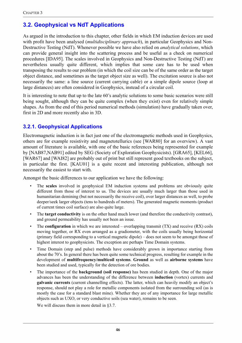
CHAPTER 3
3.2. Geophysical vs NdT Applications
As argued in the introduction to this chapter, other fields in which EM induction devices are usedwith profit have been analysed (multidisciplinary approach), in particular Geophysics and Non-Destructive Testing (NdT). Whenever possible we have also relied on analytical solutions, whichcan provide general insight into the scattering process and be useful as a check on numericalprocedures [IDA95]. The scales involved in Geophysics and Non-Destructive Testing (NdT) arenevertheless usually quite different, which implies that some care has to be used whentransposing the results to our problem (in which the coil size can be of the same order as the targetobject distance, and sometimes as the target object size as well). The excitation source is also notnecessarily the same: a line source (current carrying cable) or a simple dipole source (loop atlarge distances) are often considered in Geophysics, instead of a circular coil.
It is interesting to note that up to the late 60’s analytic solutions to some basic scenarios were stillbeing sought, although they can be quite complex (when they exist) even for relatively simpleshapes. As from the end of this period numerical methods (simulation) have gradually taken over,first in 2D and more recently also in 3D.
3.2.1. Geophysical ApplicationsElectromagnetic induction is in fact just one of the electromagnetic methods used in Geophysics,others are for example resistivity and magnetotellurics (see [WAR80] for an overview). A vastamount of literature is available, with one of the basic references being represented for exampleby [NAB87,NAB91] edited by SEG (Society of Exploration Geophysicists). [GRA65], [KEL66],[WAR67] and [WAI82] are probably out of print but still represent good textbooks on the subject,in particular the first. [KAU01] is a quite recent and interesting publication, although notnecessarily the easiest to start with.
Amongst the basic differences to our application we have the following:• The scales involved in geophysical EM induction systems and problems are obviously quite
different from those of interest to us. The devices are usually much larger than those used inhumanitarian demining (but not necessarily the receive coil), over larger distances as well, to probedeeper/seek larger objects (tens to hundreds of meters). The generated magnetic moments (productof current times coil surface) are also quite large.
• The target conductivity is on the other hand much lower (and therefore the conductivity contrast),and ground permeability has usually not been an issue.
• The configuration in which we are interested – overlapping transmit (TX) and receive (RX) coilsmoving together, or RX even arranged as a gradiometer, with the coils usually being horizontal(primary field corresponding to a vertical magnetic dipole) – does not seem to be amongst those ofhighest interest to geophysicists. The exception are perhaps Time Domain systems.
• Time Domain (step and pulse) methods have considerably grown in importance starting fromabout the 70’s. In general there has been quite some technical progress, resulting for example in thedevelopment of multifrequency/multicoil systems. Ground as well as airborne systems havebeen studied and used, typically for the detection of ore bodies.
• The importance of the background (soil response) has been studied in depth. One of the majoradvances has been the understanding of the difference between induction (vortex) currents andgalvanic currents (current channelling effects). The latter, which can heavily modify an object’sresponse, should not play a role for metallic components isolated from the surrounding soil (as ismostly the case for a standard blast mine). Whether they are of any importance for large metallicobjects such as UXO, or very conductive soils (sea water), remains to be seen.We will discuss them in more detail in §3.7.
46

EMI MODELLING AND ANALYTICAL SOLUTIONS
• A very conductive soil, or a very conductive overburden (earth above the target, not necessarily incontact with it) can also influence the target’s response, by rotating its phase and, depending on theconductivity, also attenuating its amplitude. This is likely not to represent a problem in ourapplication, perhaps with the exception of deep objects and/or large background conductivity.We will discuss these aspects in §4.4.
• Frequency differencing methods have been used to reduce the so-called “geologic noise”, in amanner similar to what implemented in the Förster Minex metal detector. They will be the subjectof §4.3.
3.2.2. EM Non-Destructive Testing (NdT)EM induction sensors have been in use for quite some time – with pioneering work carried out byFörster at the beginning of the fifties – for the analysis of metallic objects, typically rods, bars,sheets. Induction sensors have been used on one hand for the analysis of their electricalparameters (conductivity, permeability), and the other to check in a non-destructive way anobject’s integrity (cracks, defects). Ferromagnetic objects with high permeability are quitefrequent, to the contrary of geophysical scenarios.
A trend similar to the one in Geophysics towards numerical solutions [IDA95] has taken place.Basic literature is represented for example by [LIB71], [McM86], [VUI94], [BLI97] and somearticles in the [SHA] series.
47

CHAPTER 3
3.3. General Form of an Object’s EM Response
As briefly pointed out in §3.1, although the equations governing F(α) in the general case are morecomplicated than Eq. (3.4), the response characteristics of a simple circuit model are actuallysimilar to those of more realistic models, some of which we will analyse in the following. Anumber of conclusions on the general form of an object’s EM response can therefore already bedrawn.
3.3.1. General Form of the Response Parameter[GRA65] performs an interesting dimensional analysis to identify which are the parametersaffecting a system’s response (in general), and shows that the quantity replacing the adimensionalresponse parameter α, also called induction number, will be of the form:
(3.5)
The linear dimensions lj and lk are those which effectively control the volume of the eddy currentcirculation. We will see later on that their product is a2 in the case of a sphere (a= radius),whereas it is of the form t2 for a sheet of thickness t, or ta for a disk of thickness t and radius a.Table 3.1 shows some typical examples [WAR67]. The loops mentioned in the 5th and 6th rowsare horizontal coplanar, where ρ is the loop spacing and h is their height above ground, but theresults are extensible to other configurations. Note in particular the difference between the loopson (σµωρ2) and (well) above (σµωh2) the ground; there is evidently an intermediate regimewhere both factors must enter. The last row deals with the case of a single loop of radius r, towhich we will come back in Chapter 4.
Eq. (3.5) is sometimes approximated by saying that EM systems respond to σ l2 (l is an averagelinear dimension of the body), when the average dimension is small in relation to the scale valueof the system (overall or largest system dimension) [GRA65].
3.3.2. Spherical Conductor with Axial SymmetryThe special case of the primary magnetic field Hprim and a finite size conductive bodycharacterised by axial symmetry with a common axis is treated in [KAU01, §3.4]. Examplesinclude a spheroid in a uniform field (with Hprim along one of the symmetry axes), a verticalcylinder coaxial with a coil, or a horizontal disk in a uniform vertical field. Note that in thesecases no surface electrical charges develop (and therefore no galvanic currents, see §3.7).
The resulting expression in cylindrical coordinates for the induced current density and theassociated H and E fields exhibits discrete singularities, or poles, along the imaginary axis of thecomplex ω plane, the locations of which control the principal features of the frequency spectrum
Object or System Response Parameter
Sphere, uniform field σµωa2
Cylinder, uniform field σµωa2
Disk, uniform field σµωtaThin sheet σµωt2
Horizontal loops on homogeneous earth σµωρ2
Horizontal loops above homogeneous earth(system raised well above the earth: h>ρ)
σµωh2
Horizontal loop on homogeneous earth σµωr2
Table 3.1: Examples of response parameters for typical scenarios of interest [WAR67])
α σµωljlk=
48

EMI MODELLING AND ANALYTICAL SOLUTIONS
(simple sum of fractions) or equivalently of the transient decay (simple sum of exponential):
(3.6)
(3.7)
where the poles are given by
. (3.8)
a represents the observation point, b is an arbitrary geometrical parameter of the body (e.g. theradius, one of the semi-axes, etc.), σ0 is the conductivity at a specific point. The adimensionalcoefficients (dn, fn) are basically coupling coefficients which determine the strength with whicheach mode is excited, and therefore the final response spectrum. As such they depend on theproblem geometry as well as on the dimensions and shape of the conductive body25.
3.3.3. General Confined Conductor Response FunctionIt can be shown that the previous results remain valid for the more general case of a confinedconductor. Simplifying, the resulting representation of the induced currents consists of a set ofcurrent patterns, called eigencurrents26 and in general infinite, each having a fixed geometry andrepresenting a non-interacting (isolated) current which has the electrical properties of a simpleloop with a pole at ωn (or equivalently, with a time constant τn=1/ωn). The eigencurrent set formsa basis into which any finite sized vortex of eddy currents can be decomposed.
Each eigencurrent depends only on the object’s conductivity distribution, not on the primaryfield. The corresponding coupling coefficient cn, which determines the excitation level of the ntheigencurrent and therefore the overall response function F(ω), does however depend on thesource field [KAU78, NAB91 p.929, WES91]. Note that the poles are purely imaginary27: thedenominator is equal to zero for ω=iωn (ωn real >0).
(3.9)
The corresponding time domain expression is again an infinite sum of damped exponentials. Theconstant offset a is necessary to take into account the response of ferromagnetic objects.
It is intuitively clear that the eigencurrents are similar to (resonating) modes. The principal modeis the eigencurrent with the lowest frequency (ω1), or equivalently with the longest time constant(τ1=1/ω1), when the series is enumerated in order of increasing frequencies, and is usually the onewhich dominates. Indeed, the coupling coefficients cn form a convergent series: their magnitudedecreases systematically, but not necessarily uniformly, with n. The relationship between the latestage behaviour in the time domain and the low-frequency part in the frequency domain isdiscussed in detail in [KAU01, pp.222-225].
25. We will see in §3.4.5 that in some cases the geometry dependence uncouples, e.g. for a sphere.26. Because they independently satisfy the homogenous (source-free) differential equations for the fields in a given
conductivity distribution.27. [KAU01] uses poles along the negative imaginary axis (p. 204).
Hz ω a,( ) H0z dnziω
qn σ0⁄ µb2( ) iω–------------------------------------------
n 1=
∞
∑ , Hr ω a,( ) H0z drziω
qn σ0⁄ µb2( ) iω–------------------------------------------
n 1=
∞
∑==
Eφ ω a,( ) iωH0zµb fniω
qn σ0⁄ µb2( ) iω–------------------------------------------
n 1=
∞
∑=
ω iωn iqn
σ0µb2--------------- with q1 q2 q3 …< < <–= =
F ω( ) a cnω2 iωωn+
ω2 ωn2+
-------------------------
n 1=
∞
∑+ a cnω
ω iωn–----------------
n 1=
∞
∑+= =
49

CHAPTER 3
The previously described behaviour of the response function does represent the essence of thischapter’s contents, which will put the emphasis on an object’s spectral response, rather than on itsgeometry and signal strength. A few important remarks have however to be made:
1) In the case of a non-spherical object each of the object’s principal axes will usually support itsown system of eigencurrents, and therefore have a different response function.2) A non-uniform primary field can be expressed as a multipole expansion about the principalaxes of the target object, whereby each term of the expansion creates its own system ofeigencurrents similar to Eq. (3.9). The spectral response of each of the multipole terms of theinduced (secondary) field is therefore the sum of many eigencurrents. However, when we are farfrom the object only a reduced number of multipole terms is necessary.3) A target is usually analysed (“illuminated”) from different views, for example by moving alonga line over it. The configuration of the primary field at the target does therefore change, and fromwhat just discussed at 1) and 2) the resulting eddy current patterns as well. Basically differentmodes can be excited, and their excitation strengths vary. This is particularly true for elongatedferromagnetic objects.The overall response can also depend on the observation point (if far or close to the object forexample) [WES91].
These issues and their actual importance will become clearer when looking at concrete examples,and later on at the experimental data.
3.3.4. Multiple Conductors (composite objects and coupling effects)In a scenario featuring multiple conductive objects the total effect might not be, in general, asimple sum of the individual responses, depending on how well the objects are coupled (inductiveinteraction).
The case of coupled loops is described in [GRA65], which also studies the response of adisseminated conductor. The latter could serve as a basis, albeit probably with a number ofrestrictions28, for the estimation of the response of an object mostly composed of a large numberof small pieces such as a bounding fragmentation mine (e.g. the Valmara 69, which has a plasticenvelope).
[NEG72] have considered the 2D problem of a cylindrical body surrounded by a coaxial shell, inthe field of a line source. This covers for example the case of hollow cylinders. Complexphenomena can emerge for such a composite object, e.g. screening effects, especially at highfrequency, due to the skin effect in the shell. This constitutes one of the few examples of situationsin which the phase does not necessarily decrease monotonically with frequency.
After having discussed the general form of an object’s EM response we will now analyse in detailtwo models for which exact solutions exist, namely the sphere and the infinite cylinder transverseto the primary magnetic field.
28. Each particle, such as a small sphere, can probably not be considered as being isolated from its neighbours.
50

EMI MODELLING AND ANALYTICAL SOLUTIONS
3.4. The Response of a Homogeneous Sphere
The classical problem of a homogeneous sphere in the field of a dipole or a loop has been studiedfor quite some time, and its solution represents a good approximation to the response of small,regular objects. Exact solutions exist in a number of cases. We will first comment on the possiblescenarios and introduce the quasi-static approximation, to then consider in detail the situation of asphere in the field of a coaxial coil and the expansion in multipole terms of its response.
3.4.1. General ConsiderationsThe response of a homogenous sphere has been studied in detail in a number of differentscenarios. Broadly speaking we can categorize them as follows:
• Different incident (primary) magnetic field patterns, such as homogeneous, dipolar, or multipolar(e.g. with the sphere on a coil’s axis).
• Different surrounding medium, such as (in increasing order of realism and complexity): Emptyspace (i.e. isolated target), embedded in a full space (infinite external medium, also called wholespace), approximations to the exact half space solution (e.g. half space response + free spacetarget, or first order interaction), emdedded in a half space (buried object, full interaction).
We note in passing that different conventions are in use for the time factor (for alternating fields),which is usually omitted in intermediate calculations, and the propagation constant. For example,[WAR67] uses a time factor of e–iωt and his propagation constant is ;[WAI82] uses eiωt and ; [WAR87] uses eiωt and . Thepropagation constant is also called γ.
Figure 3.3: Different incident (primary) magnetic field patterns (valid for a general target).
Figure 3.4: Different Surrounding Medium scenarios (valid for a general target).
UNIFORM FIELD RADIAL/TRANSVERSE
σ, µ, ε, a
LOOP (CIRCULAR)
σ, µ, ε, a
DIPOLE
mt
mr
σ, µ, ε, a
EMPTY SPACE
σ, µ, ε, a
σ, µ, ε¦EXT = 0FULL SPACE
σ, µ, ε, a
σ, µ, ε¦EXT HALF SPACE
σ, µ, ε, a
σ, µ, ε¦SOIL
AIRINTERFACE
k2 iσiµiω εiµiω2+=
k2 iσiµiω εiµiω2–= k2 iσiµiω εiµiω
2–( )–=
51

CHAPTER 3
3.4.2. Homogeneous Sphere in a Homogeneous Full SpaceWe will start the analysis of the response of the homogenous sphere by considering the case of thetarget embedded in a homogenous full space, without however entering into the full details of theeffect of the host medium on the secondary field. It is usually assumed that the host medium andthe target response can be simply added as if they were non-interacting; this will be discussed inmore detail in §3.7 (see Eq. (3.55)).
The main ideas behind the exact solution of the problem of a sphere embedded in a half space,more realistic but even more difficult to solve than the full space approximation used here, areavailable in A3.1.
Sphere in the Field of a Magnetic DipoleSolutions to this configuration are available for instance in [WAR87] and [KAU01]. The firstreference in particular deals with the problem in its Section 6, expressing the fields in terms ofTMr and TEr modes (radial Transverse Magnetic and Transverse Electric modes, respectively).The magnetic dipole can be oriented in either the radial or the transversal direction (see alsoFigure 3.3); indeed, an arbitrarily oriented dipole can be resolved into a combination of atransverse and a radial dipole.
Quasi-Static ApproximationThe solutions are then simplified, as is often the case when dealing with this type ofelectromagnetic problems, in the quasi-static approximation (low frequency approximation), i.e.assuming that the distances involved (in this case the dipole-sphere r0 and observer-spheredistance r, as well as the sphere radius a) are much less than a wavelength29, and assuming thatdisplacement currents can be neglected. The quasi-static approximation can be expressed as:
(3.10)
with k1 being the wave number in the external medium, whereas neglecting displacement currentsis possible when
(3.11)
in which case the propagation constant also simplifies to (the dependence on the dielectricconstant ε disappears):
(3.12)
Eq. (3.10) is usually well satisfied, with the possible exception of high conductivity soils towardsthe higher frequency end (although only k is tabulated in Table 3.2, one can assume a maximumvalue of a, r and r0 of the order of 1 m for our application, thus having an immediate idea of theapproximation’s validity).
Eq. (3.11) is very well satisfied in metals: indeed, even in the case of poor conductivity (σ=105 S/m say), εω/σ has a value of only 5.6 10–10 at 1 MHz. It usually also holds true in the case of soil,although this could not be the case for very low conductivity soils towards the high frequency end(see Table 3.2). Most soils are probably in the 10–3-1 S/m range, with the possible exception ofdry sand or where rocky conditions are prevalent [McF89].
29. Or equivalently, that the skin depth in the external medium is much larger than the distances involved and thesphere size. See also Eq. (3.15).
k1a , k1r , k1r0 1«
µεω2 µσω« σ⇒ εω»
k2 iσµω , i 1–= =
52

EMI MODELLING AND ANALYTICAL SOLUTIONS
The dielectric constant of geologic materials varies from 1 to about 81 (pure water), and is usuallystrongly related to water content. In Table 3.2 we have taken a typical value of εr=10, whichmight have to be increased for water saturated soils [McF89]. The relative permeability of soils isseldom greatly different from unity [WAR67], see also Table 3.3; in most cases it is determinedby the magnetite content, with massive magnetite having µr=5. Nevertheless, as discussed inChapter 2, this can significantly impact the performance of metal detectors. The conductivity canreach a few S/m in salt water.
Physically speaking these approximations mean that the magnetic field at any point in themedium is defined by the instantaneous values of current density throughout the conductingmedium, and can be calculated using only the Biot-Savart law30 (like in the case of a staticmagnetic field). Also, the propagation time for the electromagnetic energy can be neglected, i.e. itis assumed that the field travels instantaneously (propagation effects not considered). In this casethe wave equations for the electric and magnetic fields reduce, when displacement currents can beneglected, to diffusion equations (they describe the penetration of energy, but do not take intoaccount wave propagation) [KAU01,§2.5].
The quasi-static approximation is therefore valid when conduction currents dominate overdisplacement currents in a conducting medium, and when the arrival time for a signal in aninsulator is much less than the duration of a measurement, or the period of the observedoscillations.
Sphere in the Field of a LoopThis is for example dealt with in [KAU01,§5.2], considering an external medium with µext=µ0.We will look at this geometry in the next paragraph, using however the quasi-staticapproximation, which is sufficient for our purposes, rather than the exact solution.
Soilconductivity σ (S/m) εω/σ @ 1kHz εω/σ @ 1MHz k @ 1 kHz k @ 1 MHz δ @ 1 kHz δ @ 1 MHz
high 1 5.6×10⁻⁷ 5.6×10⁻⁴ 0.089 2.8 15.8 0.5
low 10–3 5.6×10⁻⁴ 0.56 2.8×10⁻³ 0.089 500 15.8
very low 10–5 5.6×10⁻² 56 2.8×10⁻⁴ 8.9×10⁻³ 5×10³ 158
Table 3.2: Values of εω/σ, k (in m–1) and δ (in m) for some soil scenarios (ε=10ε0, µ=µ0 throughout)
Mineral Relative Permeability µr
Magnetite 5.0Pyrrhotite 2.55Ilmenite 1.55Hematite 1.053
Pyrite 1.0015
Table 3.3: Relative Permeability values for some ferromag. minerals (in units of µ0) (from [KEL66], Table 14)
30. The quadrature and in-phase components of the secondary magnetic field will therefore be generated by thecorresponding components of the induced currents, and have similar frequency responses [KAU01,§2.4.6.2].
53

CHAPTER 3
3.4.3. Homogeneous Sphere in the Field of a Coaxial CoilWe will follow here the formulation of [McF89], with early solutions in Geophysics going back atleast to the early fifties [WAI53] ([WON98] lists several classical papers by Wait on the subject).It is interesting to note that the problem has also been treated separately in NdT, e.g. in [VEI65],which presents the analytical details of a number of classical problems (coaxial circular coils inthe presence of planar, cylindrical and spherical conductors, in free space), relying on themagnetic vector potential formulation and using appropriate boundary conditions. Extensions to acoil encircling two concentric, spherical shells (in free space) of finite (σ,µ), is provided in[LUQ70], with extensions to coil of finite sizes. No numerical results are reported in these twoNdT references.
The response of a homogeneous sphere of radius a, conductivity σ and permeability µ(µ=µ0µr), placed in the field of a circular transmit coil of radius RT, as measured by a circularreceive coil of radius RS, can be calculated exactly (in the quasi-static approximation describedabove and neglecting displacement currents). The coils are coaxial and placed on the sphere’saxis at a distance dT and dS from the sphere’s centre as shown in Figure 3.5.
The operating frequency is ω, and the transmit coil is traversed by a constant current I. Timedependence is implicitly assumed as eiωt and omitted in the following.
This analysis has the advantage of using a realistic geometry for small nearby objects; it alsoreduces in the limit to the commonly used uniform primary field or dipole approximation. Notethat throughout this analysis we will assume a constant relative permeability µr. In fact this is farfrom obvious as µr can depend on the operating frequency and in particular on the strength of theapplied field [SOW98b].
The primary field can be expanded in spherical harmonics, and each generates a sphericalharmonic in the secondary field for the same index n. It can therefore be shown [McF89] that theinduced voltage can be written as a sum of products of geometry and frequency dependentterms as follows ( are associated Legendre polynomials and In+1/2(ka), In-1/2(ka) are modifiedBessel functions of the first kind; see also A3.3):
(3.13)
Figure 3.5: Geometry for the calculation of the response of a sphere in the field of a coil (adapted from [McF89]). Size and position of the primary and secondary loops are not representative.
V s( )
SECONDARYr0
Z
Y
dT
σ, µ, a
X
RT
RS
dS
PRIMARY LOOP
LOOP
V s( )
Pn1
V s( ) 2πiµ0IωRSRT
dT2 RT
2+( )1 2⁄
------------------------------ a2n 1+
2n n 1+( )-----------------------
Pn1 dT dT
2 RT2+[ ]
1 2⁄⁄( )Pn
1 dS dS2 RS
2+[ ]1 2⁄
⁄( )
dT2 RT
2+( )n 2⁄
dS2 RS
2+( )n 1+( ) 2⁄
-------------------------------------------------------------------------------------------------------χn ka( )
n 1=
∞
∑=
54

EMI MODELLING AND ANALYTICAL SOLUTIONS
(3.14)
(3.15)
The adimensional expression , which plays a role similar to theresponse function F(α) previously encountered, contains all the frequency dependence (apartfrom the external ω factor) as well as the dependence on the object properties (apart from thea2n+1 term). The response parameter is now k2a2=iσµωa2=iα (adimensional and purelyimaginary, with µ=µ0µr) rather than α=ωL/R; it is related to the skin depth δ as indicated in Eq.(3.15).
There are actually a number of different ways in which the response function can be expressed,using for example spherical modified Bessel functions instead of modified Bessel functions, andtheir derivatives. We will here only point out that the χn listed above are equivalent to the Rn(reflection) coefficients in Wait’s original article [WAI53], which are in turn defined as Sn in[WAI60], rTEr in [WAR87], etc.
Note that this response function is parametrized by the sphere’s relative permeability µr. In factwe have implicitly assumed µext=µ0, otherwise one has to replace µr with the permeabilitycontrast K=µsph/µext. Note also that the external medium conductivity does not appear any more inthe quantities of interest.
The rest of Eq. (3.13) contains the geometrical factors, i.e. the relative geometry of the sphere andthe transmit and receive coils. We shall define in particular as “geometry term” gn theadimensional expression to the right of the sum sign, which depends on n:
(3.16)
Note also the presence of the ω factor, which means that the induced voltage grows linearly withfrequency (apart from the behaviour). Concerning the transmit current I, from a practicalpoint of view it might not be easy to keep it constant when driving the transmit coil at constantvoltage, as its impedance (RTransmit+iωLT) grows when increasing ω.
Table 3.4 lists typical values of the response parameter α=σµωa2 for spheres of radius 1 mm, 5mm, 1 cm and 5 cm, at the two operating frequencies of the Förster Minex metal detector (f1=2.4kHz and f2=19.2 kHz), which are typical of the frequency range of interest. Note that α increasesquadratically with the object radius, and linearly with its conductivity and permeability, and withthe frequency. This is why the highest values for a given sphere size and frequency are those ofpermeable steel, followed by copper. As a rule of thumb we can say that small values of a (smallobjects), low operating frequency and low conductivity tend to reduce α, the opposite whendealing with large objects, high operating frequency and good conductors or permeable objects.
Material σ (107 S/m) µr α for a=1mm α for a=5mm α for a=1cm α for a=5cm
Copper 5.8 1 1.10 (8.8) 27 (2.2×10²) 1.10×10² (8.8×10²) 2.7×10³ (2.2×10⁴)Aluminium 3.54 1 0.67 (5.4) 17 (1.3×10²) 0.67×10² (5.4×10²) 1.7×10³ (1.3×10⁴)
Brass (yellow) 1.5 1 0.28 (2.2) 7.1 (57) 0.28×10² (2.2×10²) 0.71×10³ (5.7×10³)Steel (typical) 0.63 150 18 (1.4×10²) 4.5×10² (3.6×10³) 1.8×10³ (1.4×10⁴) 4.5×10⁴ (3.6×10⁵)
Table 3.4: Typical conductivity, relative permeability, and response parameter α for spheres of different sizes at f1=2.4 kHz (and f2=19.2 kHz) (using the conductors tabulated in Table 2.1)
with χn ka( ) Xn ka( ) iYn ka( )+n 1+( )µr n+[ ]In 1 2⁄+ ka( ) kaIn 1 2⁄– ka( )–n µr 1–( )In 1 2⁄+ ka( ) kaIn 1 2⁄– ka( )+--------------------------------------------------------------------------------------------------------= =
and k2a2 iσµωa2 iα 2ia2
δ2-----= = =
χn ka( ) Xn ka( ) iYn ka( )+=
gn dT RT dS RS a;, , ,( ) a2n 1+
2n n 1+( )-----------------------
Pn1 dT dT
2 RT2+[ ]
1 2⁄⁄( )Pn
1 dS dS2 RS
2+[ ]1 2⁄
⁄( )
dT2 RT
2+( )n 2⁄
dS2 RS
2+( )n 1+( ) 2⁄
------------------------------------------------------------------------------------------------------- .=
χn ka( )
55

CHAPTER 3
Series Expansion of the Response FunctionEach term χn of the response function can actually be expanded in a series, containing a sum ofsimple fractions [KAU01, §3.3], along the lines of what discussed in §3.3 (eigencurrents) and inparticular in Eq. (3.9). The poles ωns:
(3.17)
are again situated on the imaginary axis (negative values are due to the convention in [KAU01]),with the coefficients qns having the following properties:
(3.18)
A detailed expression will be given in Eq. (3.25) for the dipole approximation, to which in factthe q1s coefficients correspond.
We will now analyse in more detail Eq. (3.13) for the most important cases.
3.4.4. Sphere in the Field of a Coaxial Coil – Multipole Terms (geometry, gn)
Higher order terms decrease more rapidly with distance than lower order terms (this is easier tosee for d=dT=dS, the coplanar case). Conversely, as the coils approach the sphere higher orderterms become significant and the secondary field in the sphere receives contributions from higherorder multipoles. The multipole terms do indeed scale as:
(3.19)
which is similar but not equal to the well known behaviour of a sphere in the field of a magneticdipole (see for example [GRA65]), whose multipole coefficients scale approximately as a2/r2
[(n+2)/n] for a sphere of radius a at a distance r.
Coming back to our case, the contribution from higher order multipoles is illustrated in Figure3.6, representing the geometry term gn of Eq. (3.16) for n=1 to n=4 in the case of overlappingcoils (d=dT=dS and R=RT=RS) and a rather large sphere, of radius a equal to the coil radius R(a=R=0.1). The case of a small sphere will be analysed later. Units are in fact indifferent, butthinking in terms of meters for example provides realistic size and depth estimates. The plots areinteresting for us for d>a (top of the sphere below the coil); there the n=1 term clearly dominates,with an initially substantial contribution from the n=2 term (up to a distance of 2-3 times thesphere diameter) and a smaller contribution for n=3. Note that the gn term scales – identical plotsare obtained when multiplying a and R by a factor and modifying the distance plotting rangelimits by the same amount – as can be easily seen when rewriting gn in terms of a/d and R/d.
3.4.4.1. Multipole Terms for a Non-Ferromagnetic Object (χn for µr=1)
Figure 3.7 illustrates the behaviour of the first four terms of the response function χ for a non-ferromagnetic object (µr=1). The phase has in fact been calculated over iχ (compare also with Eq.(3.13)) in order to reproduce the overall phase of the induced voltage, rather than the phase of theinduced currents which generate the secondary field. The multiplication by i is due to timedifferentiation of the eiωt factor ( with and ), and isequivalent to a counter-clockwise rotation of 90° in the complex plane (i.e. Re(iχ)=–Im(χ) andIm(iχ)= Re(χ)).
ωnsiqns
σµa2-------------–=
q1s π2s2 ; qn s, qn s 1+, ; qn s, qn 1+ s, ; qn 1,2n 5+( ) 2n 1+( )
2-----------------------------------------≅<<=
gn 1+gn
------------ nn 2+------------ a2
rTrS----------
Pn 1+1 rT( )Pn 1+
1 rS( )
Pn1 rT( )Pn
1 rS( )---------------------------------------------- with rT
dT
dT2 RT
2+[ ]1 2⁄
------------------------------ , rSdS
dS2 RS
2+[ ]1 2⁄
------------------------------= = =
V s( ) Φ∂ t∂⁄–= Φ Bsec Sd⋅∫= Bsec eiωt∝
56
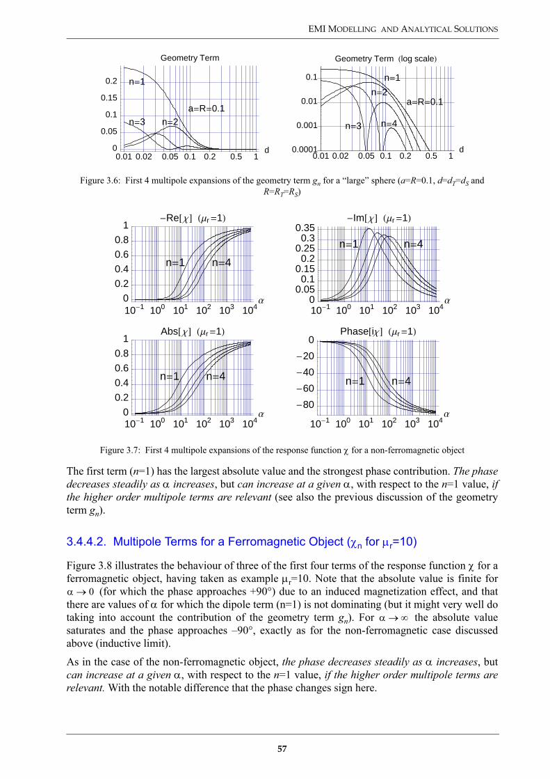
EMI MODELLING AND ANALYTICAL SOLUTIONS
The first term (n=1) has the largest absolute value and the strongest phase contribution. The phasedecreases steadily as α increases, but can increase at a given α, with respect to the n=1 value, ifthe higher order multipole terms are relevant (see also the previous discussion of the geometryterm gn).
3.4.4.2. Multipole Terms for a Ferromagnetic Object (χn for µr=10)
Figure 3.8 illustrates the behaviour of three of the first four terms of the response function χ for aferromagnetic object, having taken as example µr=10. Note that the absolute value is finite for
(for which the phase approaches +90°) due to an induced magnetization effect, and thatthere are values of α for which the dipole term (n=1) is not dominating (but it might very well dotaking into account the contribution of the geometry term gn). For the absolute valuesaturates and the phase approaches –90°, exactly as for the non-ferromagnetic case discussedabove (inductive limit).
As in the case of the non-ferromagnetic object, the phase decreases steadily as α increases, butcan increase at a given α, with respect to the n=1 value, if the higher order multipole terms arerelevant. With the notable difference that the phase changes sign here.
Figure 3.6: First 4 multipole expansions of the geometry term gn for a “large” sphere (a=R=0.1, d=dT=dS and R=RT=RS)
Figure 3.7: First 4 multipole expansions of the response function χ for a non-ferromagnetic object
0.01 0.02 0.05 0.1 0.2 0.5 1d0
0.05
0.1
0.15
0.2
Geometry Term
n�1
n�2n�3a�R�0.1
0.01 0.02 0.05 0.1 0.2 0.5 1d0.0001
0.001
0.01
0.1
Geometry Term �log scale�
n�2
n�3 n�4
a�R�0.1
n�1
10�1 100 101 102 103 104Α0
0.2
0.4
0.6
0.8
1Abs�Χ� �Μr�1�
n�1 n�4
10�1 100 101 102 103 104Α
�80
�60
�40
�20
0Phase�iΧ� �Μr�1�
n�1 n�4
10�1 100 101 102 103 104Α0
0.2
0.4
0.6
0.8
1�Re�Χ� �Μr�1�
n�1 n�4
10�1 100 101 102 103 104Α0
0.050.1
0.150.2
0.250.3
0.35�Im�Χ� �Μr�1�
n�1 n�4
α 0→
α ∞→
57

CHAPTER 3
3.4.5. Dipole Approximation (n=1) – General ConsiderationsIf the sphere is far from the coils compared to its size (d>>a), or much smaller than the coildiameter (a<<R), it only “sees” a homogeneous (uniform) primary field and only the first term(n=1) is relevant (Dipole Approximation). This is illustrated in Figure 3.9, which shows thegeometry dependent term for n=1 and n=2 in the case of overlapping coils (d=dT=dS andR=RT=RS) and a small sphere (a=0.01=1/10 R).
In this case the sphere behaves like a simple magnetic dipole with magnetic moment m ( is theunit vector in the z direction):
(3.20)
(3.21)
(3.22)
where has been defined in Eq. (3.14) and H0 is the transmit field at thesphere’s centre. Here we have again implicitly assumed µext=µ0.
The induced magnetic moment m of a sphere in the dipole approximation is in fact alwaysaligned along the transmit (or primary) field HT, i.e. we can simply replace with HT in Eq.(3.20). It is also worthwhile to note that the sphere’s (dipole) phase response X+iY depends on itsparameters (µ, σ, a) and on ω, but not on the problem’s geometry (i.e. the sphere’s position withrespect to the coils), and is therefore constant for a given object (as long as µr does not changeobviously) and working frequency ω [BAR96]. As we have seen this is not necessarily true whenhigher order multipole contributions are relevant.
Figure 3.8: First multipole expansions (n=1, 2, 4) of the response function χ for a ferromagnetic object (µr=10)
Figure 3.9: First 2 multipole expansions of the geometry term gn for a “small” sphere (a=0.01=1/10 R, d=dT=dS and R=RT=RS)
101 102 103 104 105Α
0.20.40.60.8
11.21.41.6
Abs�Χ� �Μr�10�
n�1n�2
n�4
100 101 102 103 104 105Α
�75�50�25
0255075
Phase�iΧ� �Μr�10�
n�1 n�4
0.01 0.02 0.05 0.1 0.2 0.5 1d0
0.2
0.4
0.6
0.8
x 2.5 10�4Geometry Term �n�1�
a�0.01, R�0.1
0.01 0.02 0.05 0.1 0.2 0.5 1d0
0.0005
0.001
0.0015
0.002
0.0025
x 2.5 10�4Geometry Term �n�2�
a�0.01, R�0.1
z
m 2πa3H0 X iY+( ) z–=
with H0I2---
RT2
r03------ , r0 dT
2 RT2+= and =
X iYµ0 1 k2a2+( ) 2µ+[ ] ka( ) 2µ µ0+( )ka ka( )cosh–sinh
µ0 1 k2a2+( ) µ–[ ] ka( ) µ µ0–( )ka ka( )cosh+sinh-----------------------------------------------------------------------------------------------------------------------------------=+ χ1 ka( ) .–=
χ1 ka( ) X1 ka( ) iY1 ka( )+=
z
58

EMI MODELLING AND ANALYTICAL SOLUTIONS
Table 3.5 lists values (in degrees) of the phase of the induced voltage in the dipole approximationfor the response parameter (α=σµωa2) values of Table 3.4, again at f1=2.4 kHz and f2=19.2 kHz.
Induced Voltage in the Dipole ApproximationThe overall expression of the induced voltage reduces in the dipole approximation to:
(3.23)
Apart from the already stressed direct proportionality to the frequency ω, we also recognize thetypical dependence of the magnetic field generated along a coil’s axis, the term corresponding to the transmit (or primary) field and the term to the magnetic fluxin the receive coil31.
Induced Voltage for Overlapping CoilsIn the case of overlapping coils (d=dT=dS and R=RT=RS) the previous expression becomes:
(3.24)
In the case of a sphere in homogenous primary field the induced currents are circular and flow inplanes perpendicular to the direction of the inducing field.
Series Expansion of the Response FunctionThe response function in the dipole approximation can be expressed as a series, containing a sumof simple fractions, along the lines of what discussed in §3.3 (eigencurrents) and in particular inEq. (3.9). For a non-ferromagnetic object [KAU01, §3.1]:
(3.25)
The poles on the imaginary axis32 are here at:
(3.26)
Material Phase for a=1mm Phase for a=5mm Phase for a=1cm Phase for a=5cmCopper –6.0 (–38.8) –63.3 (–81.4) –77.6 (–85.8) –87.6 (–89.2)
Aluminium –3.7 (–26.8) –54.8 (–78.7) –73.9 (–84.6) –87.0 (–88.9)Brass (yellow) –1.5 (–11.8) –33.3 (–72.4) –63.8 (–81.4) –85.3 (–88.4)Steel (typical)* +88.4 (+85.4) +81.8 (+68.2) +74.2 (+49.2) +18.4 (–52.8)
Table 3.5: Phase of induced voltage in the dipole approximation at f1=2.4 kHz (and f2=19.2 kHz) for spheres of different sizes (*µr=150) (see also Table 3.4)
31. Or equivalently corresponding, using reciprocity arguments, to the field which would be produced by the receivecoil at the object location.
32. The poles are, according to the convention of [KAU01] (e–iωt time dependence), on the negative imaginary axis.X is therefore negative rather than positive as in our case.
V s( )
V s( )n 1= 2πiµ0Iωa3
4-----RT
2
dT2 RT
2+( )3 2⁄
------------------------------RS
2
dS2 RS
2+( )3 2⁄
------------------------------ X1 ka( ) iY1 ka( )+( )=
RT2 dT
2 RT2+( )
3 2⁄⁄
RS2 dS
2 RS2+( )
3 2⁄⁄
V s( )n 1= 2πiµ0Iωa3
4-----R2
d2 R2+( )3 2⁄
------------------------------2
X1 ka( ) iY1 ka( )+( )=
X iY µr 1=+ 6π2----- 1
n2----- iωπ2n2 σµa2⁄( ) iω–
---------------------------------------------n 1=
∞
∑=
ω iωn i π2n2
σµa2-------------–= =
59

CHAPTER 3
with the first pole (n=1) approximately situated at a value of the response parameter at which thereal part of the response function is equal to the imaginary (crossover, see also Figure 3.10). Theirmagnitude is rapidly increasing, the corresponding coupling coefficients do however decreasewith n2.
Factorisation of the ResponseThis case, as well as that of a simple circuit previously discussed, are examples of situations inwhich the response separates explicitly into the product of a response function (physical propertyfactor) and a coupling coefficient (geometric factor), or more precisely [WAR67]:
Response = (Inducing Field) x (Size Factor) x (Physical Property Factor) x (Geometric Factor)
In such simple cases the geometry effects can be studied separately from the effects of thephysical properties (σ,µ,R) and of ω, i.e. the effect of the response parameter is independent of thesystem’s position [GRA65]. This is in general not the case for broad conductors and/orferromagnetic objects.
3.4.5.1. Dipole Approximation for a Non-Ferromagnetic Object (χ1 for µr=1)
The dipole’s approximation response function (Eq. (3.22)) further reduces, in the case of µr = 1(non-ferromagnetic object), to:
(3.27)
Its behaviour is reproduced in Figure 3.10, the term “Dipole” and being equivalent;the phase has been calculated here over (–i Dipole) in order to again reproduce the overall phaseof the induced voltage.
As expected the plots correspond to those of the first term in Figure 3.7, with the addition of theequivalent complex plane representation; they are indeed qualitatively similar to what expectedfor a simple circuit model.
Examples of working points at the Förster Minex operating frequencies are shown as circles andsquares for copper spheres of radius 1 mm (very small object) and 1 cm respectively (see alsoTable 3.4 and Table 3.5).
For the smaller object there is a very large difference in the absolute value of the responsefunction at the two frequencies, whereas for the larger one the ratio of the two absolute valuesapproaches unity33, as we are already close to the inductive limit (see Eq. (3.13)).
Considering the absolute value of the response function for non-ferromagnetic objects higheroperating frequencies are therefore favoured, which is not necessarily true when phase-basedidentification is attempted, as the phase response curve flattens when approaching –90° [TRA97](i.e. different objects tend to show similar phase behaviour when increasing the frequency). Fromthe point of view of discriminating smaller debris from larger pieces a value of the phasethreshold in the range –60° to –80° could represent a good starting point for further investigations(for non-ferromagnetic objects).
33. The overall induced voltage features in fact an additional factor ω, as we have already seen in Eq. (3.13).
X iY µr 1=+ 3 1k2a2---------- 1
3---ka( )cosh
ka ka( )sinh----------------------------–+ χ1 ka( )–µr 1=
.= =
X iY µr 1=+
60

EMI MODELLING AND ANALYTICAL SOLUTIONS
3.4.5.2. Dipole Approximation for Ferromagnetic Objects (χ1 for µr>1)
The dipole’s approximation response function (Eq. (3.22) or equivalently Eq. (3.14) with n=1) isreproduced in Figure 3.11 for two different ferromagnetic objects (µr=10 and µr=100) as well asfor µr=1 (non-ferromagnetic) for comparison. The plots for µr=10 correspond to those of the firstterm (n=1) in Figure 3.8. The complex plane representation is here shown for µr=100 only. Thebehaviour of the phase includes again the factor i in order to reproduce the overall phase of theinduced voltage. As we already pointed out, the response function for ferromagnetic objects isparametrized by µr (i.e. there is one curve for each value of µr).
Similarly to what already noted for Figure 3.10, for the absolute value saturates and thephase approaches –90°, as for the non-ferromagnetic case (inductive limit), whereas the phaseapproaches +90° and the absolute value is finite for due to an induced magnetization effect(and for ) [McF89, TRA97]. This well-known fact could be used to determineif an object with negative phase response is ferromagnetic or not, using a magnetometer ormultiple frequency measurements (with at least one frequency rather low). Indeed, from whatsaid it is clear that a single phase measure resulting in a negative value is by itself not sufficient tostate that the object is non-ferromagnetic. Still concerning the low frequency limit, note that:
Figure 3.10: First multipole term (n=1: dipole approximation) of the response function χ for a non-ferromagnetic object (µr=1).
100 200 300 400 500Α
�80
�60
�40
�20
0Phase��i Dipole� �linear scale�
10�1 100 101 102 103 104Α
�80
�60
�40
�20
0Phase��i Dipole�
10�1 100 101 102 103 104Α0
0.2
0.4
0.6
0.8
1Re, Im, Abs�Dipole�
Abs Re
Im
0.1 0.2 0.3
�1
�0.8
�0.6
�0.4
�0.2
Im��i Dipole� vs. Re ��i Dipole�
Α�0
Α�10
Α�102
Α��
(example) Copper sphere, 1mm radius: @f1@f2
1cm radius: @f1@f2
Complex plane representation
α ∞→
α 0→Abs χ[ ] 2→ µr ∞→
61

CHAPTER 3
(3.28)
as can be verified in Figure 3.11 for µr=10 (limit: 1.5) and µr=100 (limit: about 2).
It can also be noted that the peak in the quadrature component at high permeability values is:
(3.29)
For a given µr the phase decreases steadily as α increases, again with the notable difference withrespect to non-ferromagnetic objects that its sign changes. On the other hand the phase increaseswhen increasing µr whilst keeping the other object parameters (σ,a) and the operating frequencyω constant. This can be seen by moving from example from the phase response at µr=10 for agiven α1 to the corresponding phase response at µr=100 (i.e. for α2=10α1 as shown by the arrowlabelled “1” in Figure 3.11).
For a given µr the absolute value of the response function decreases as α increases and thenslowly rises again; this seems to favour lower operating frequencies34.
Figure 3.11: First multipole term (n=1: dipole approximation) of the response function χ for different ferromagnetic objects as well as for µr=1 for comparison (dashed in top plot; arrows: see text).
χα 0→lim
2 µr 1–( )2 µr+----------------------=
αPeak IM( ) σµωPeak IM( )a2 µr
2 ωPeak IM( )µr
2
σµa2-------------≅⇒≅=
100 101 102 103 104 105 106 107Α
�75
�50
�25
0
25
50
75
Phase�iΧ� �Μr�1,10,100�
Μr�1Μr�10
Μr�100
100 101 102 103 104 105 106 107Α
0.25
0.5
0.75
1
1.25
1.5
1.75
Abs�Χ� �Μr�1,10,100�
Μr�1
Μr�10
Μr�100
100 101 102 103 104 105 106 107Α
�2
�1.5
�1
�0.5
0
0.5
1�Re�Χ�,�Im�Χ� �Μr�1,10,100�
10
10
100
100
0.1 0.2 0.3 0.4 0.5 0.6
�1
�0.5
0.5
1
1.5
2Im�iΧ� vs. Re�iΧ� �Μr�100�
Α�0
Α�6 102
Α�2 103
Α�104
Α�2 104
Α�105
Α��
(example) Steel sphere (µr=100), 1mm radius: @f1@f2
1cm radius: @f1@f2
1
2
3
62

EMI MODELLING AND ANALYTICAL SOLUTIONS
If instead we increase µr whilst keeping the other object parameters (σ, a) and ω constant, at lowvalues of α the absolute value of the response function increases (follow the arrows labelled “2”and “3” in Figure 3.11). In this regime the difference between non-ferromagnetic andferromagnetic objects can be significative. Moving to higher values of α this trend is reversed.
Examples of working points at the Förster Minex operating frequencies are again shown ascircles and squares for mild steel spheres, with µr=100, of radius 1 mm (very small object) and 1cm respectively (see also Table 3.4 and Table 3.5, where the values are in fact calculated forµr=150). From the point of view of discriminating smaller debris from larger pieces a value of thephase threshold around +75° could represent a good starting point for further investigations (butin particular the case of objects with high µr values has to be studied more attentively).
3.4.6. Summary of Theoretical Analysis (Sphere)We will briefly summarize the basic findings of the previous theoretical analysis (response of ahomogenous sphere in the field of coaxial circular coils, placed on the sphere’s axis):
• The induced voltage can be expressed as the sum of an infinite number of multipole terms, whichcan be represented as the product of a geometry dependent term gn (real) and a response functionχn (complex). The latter is a function of the response parameter α=σµωa2, which depends on theobject’s properties (σ, µ, a) and on the operating frequency ω (see Eq. (3.13) to Eq. (3.15)).
• Higher order multipole components are not important if the sphere is far from the coils comparedto its size (d>>a), or much smaller than the coil diameter (a<<R) (dipole approximation,homogeneous primary field).
• Non-ferromagnetic objects behave similarly to what predicted by a simple circuit model. Thebehaviour of ferromagnetic objects is parametrized by µr; they exhibit a finite response for ,and their phase ranges from +90° to –90°. In both cases the phase decreases monotonically with α,but it can increase when higher order multipole terms are important or for increasing µr.
• In the dipole approximation the sphere’s response does not depend on its position, only on theobject’s parameters.
• Higher operating frequencies are particularly important for the detection of small non-ferromagnetic objects; the opposite tendency is true for ferromagnetic ones (thinking of theabsolute value of the response function).
• In principle one can differentiate between ferromagnetic and non-ferromagnetic objects (onlyferromagnetic objects exhibit a positive phase response). Note that a single phase measureresulting in a negative value is by itself not sufficient to state that the object is non-ferromagnetic.
These general trends should still hold also for non-spherical objects, especially for smaller onesfor which the dipole approximation is more likely to be satisfactory.
34. Again, keeping in mind that the overall induced voltage features an additional factor ω (Eq. (3.13)).
α 0→
63

CHAPTER 3
3.5. Homogenous Cylinders
Cylinders represent another shape common to several objects of interest in humanitariandemining applications, e.g. some mine strikers when considering small objects, and somemetallic mines and UXO when considering large objects. Analytical solutions can again provideinsight into the scattering process, and be useful as a check on numerical procedures [IDA95]. Wewill deal first with horizontal infinite cylinders (§3.5.1), then with objects of finite length (§3.5.2and §3.5.3).
3.5.1. Horizontal Infinite CylindersAnalytical solutions for the cylinder case have been first available in Geophysics in an idealizedsituation featuring a homogeneous infinitely long circular object (σ2,ε2,µ2) immersed in ahomogenous external medium (whole space (σ1,ε1,µ1)) with an exact solution being availablewhen the source is represented by an infinite line source of electric current running parallel to thecylinder (e.g. a cable) (2D problem) [WAI52, WAR87, KAU01, §6.4.2] as shown in Figure 3.12.They constitute a geophysical extension of the classical problem of diffraction by a circularcylinder.
It will be shown that the inductive behaviour is similar to the one of a sphere when the magneticfield is perpendicular to the cylinder’s axis.
3.5.1.1. Parallel Line Source (2D problem, exact solution)
The secondary magnetic field components in the region outside the cylinder can be written asfollows, omitting the eiωt factors (In(γia), Kn(γia) are modified Bessel functions of the first andsecond kind respectively. The cylinder is defined as ρ<a for –∞<z<∞ in cylindrical coordinates;the line source is located at (ρ0,φ0) and P is an observation point [WAI52].
The prime on a Bessel’s function denotes a derivative with respect to its argument, and K=µ2/µ1=µcyl/µext is the magnetic permeability contrast [WAI73b]:
(3.30)
Figure 3.12: Geometry for the calculation of the response of an infinite cylinder in the field of a parallel infinite line source; section view, z axis towards reader and parallel to the cylinder (adapted from [KER60]).
X
LINE SOURCEρ, φ
Y
σ2, µ2, ε2, αXCYLINDER
σ1, µ1, ε1
ρ0, φ0
H(S)
LINE SOURCE
Y
Z
ρ0φ0
ρ φP
H(S)ρ
H(S)φ
Hφs( ) I
2πρ---------- qn
n ∞–=
∞
∑–Kn γ1ρ0( )Kn γ1a( )----------------------In γ1a( )Kn' γ1ρ( )γ1ρe im φ φ0–( )–=
64

EMI MODELLING AND ANALYTICAL SOLUTIONS
(3.31)
with
(3.32)
(3.33)
where γm (m=1,2), are the usual propagation constants: and qn can beinterpreted as a reflection coefficient which determines the amplitude and phase of the secondarycylindrical waves of order n, as they are reflected from the surface of the cylinder. The secondaryfield is expressed as the sum of a field of linear multipoles.
The first expression for qn is quite rigorous and depends indeed on all electromagnetic parameters(σm,εm,µm), whereas the second is an approximation valid when the external mediumconductivity (σ1) is small (actually – quasi-static approximation already discussed [SIN73] –when ). The only dependence on the external medium parameters is now viaK. Under such an approximation the secondary magnetic field can be expressed as:
(3.34)
Note that the frequency spectrum for the secondary field will in general change depending on theobservation point position (different contributions from each multipole term).
For K=1 the reflection coefficients can be further simplified to:
(3.35)
If displacement currents within the cylinder can be neglected, we have: , andconsiderations similar to those made in the case of a sphere apply. The first four multipole termsof qn are shown in Figure 3.13 in the upper half for a non-ferromagnetic object and in the lowerhalf for a ferromagnetic object with µr=10; they are actually similar to the previously describedsolution for the sphere, i.e. a sum of similar multipole terms (linear in this case). [MIL01] alsonotes that the two solutions “converge” for high values of µr.
The case n=1 corresponds to a cylinder immersed in a homogeneous field, see [WAR67] (againcylinder embedded in a homogeneous whole space), or [WAR87]. The corresponding plots areshown in Figure 3.14.
Needless to say that the measured (experimental) quantity, i.e. the voltage at the output of thereceiver coil, is not directly the magnetic field, rather the (time derivative of the) integral of themagnetic field over the receiver’s coil surface.
The n=0 (Monopole) TermThe term in Eq. (3.34) – n=0 or monopole term – was actually missing in [WAI52] (see also[WAR87]), although the general solution was correct, and in some subsequent publications. Itdoes not appear in . This term corresponds to a unidirectional and azimuthally symmetric
Hρs( ) I
2πρ----------– qn
n ∞–=
∞
∑Kn γ1ρ0( )Kn γ1a( )----------------------In γ1a( )Kn γ1ρ( )ime im φ φ0–( )–=
qn
1η1------
In' γ1a( )In γ1a( )------------------ 1
η2------
In' γ2a( )In γ2a( )------------------–
1η1------–
Kn' γ1a( )Kn γ1a( )-------------------- 1
η2------
In' γ2a( )In γ2a( )------------------+
---------------------------------------------------------------nK γ2a
In' γ2a( )In γ2a( )------------------–
nK γ2aIn' γ2a( )In γ2a( )------------------+
-----------------------------------------≅n K 1+( )In γ2a( ) γ2a( )In 1– γ2a( )–n K 1–( )In γ2a( ) γ2a( )In 1– γ2a( )+-----------------------------------------------------------------------------------= =
ηmiµmω
σm iωεm+-------------------------
1 2⁄ iµmωγm
-------------= =
γm2 iσmµmω εmµmω2–=
γ1a , γ1ρ , γ1ρ0 1«
Hρs( ) I
2π------ qn
n 1=
∞
∑a2n
ρ0nρn 1+------------------ n φ φ0–( )[ ] , Hφ
s( ) I2π------ qn
n 1=
∞
∑a2n
ρ0nρn 1+------------------ n φ φ0–( )[ ] Hφ0
s( )+cos=sin=
qn K 1= In 1+ γ2a( ) In 1– γ2a( )⁄–=
γ2a iσ2µ2ω( )1 2⁄ a≅
Hφ0s( )
Hρs( )
65

CHAPTER 3
induced current, with the return current flowing from the ends of the cylinder through the externalmedium, which usually represents a higher impedance path with respect to the terms with n>0(the n=1 term corresponds for example to a current loop flowing within the cylinder itself, seebelow35). Its importance has been discussed and debated in a number of references.
This term is actually not negligible for the 2D case considered (infinite cylinder and line source)[SIN73]. It is also present for finite-length cylinders and line sources [SIN74], [SIN77], althoughit has been proven [WAI73a], [HIL72] that its importance is reduced by the truncation of thecylinder (this last comment also applied to a point dipole source as discussed in [WAI60]; see alsobelow). Note that it does however not arise when considering a (purely magnetic) homogenoustransversal primary field (see [WAR67] or [WAR87]).
Figure 3.13: First 4 multipole expansions of the response function qn for a non-ferromagnetic (µr=1, top) and a ferromagnetic cylinder (µr=10, bottom)
35. The higher order harmonics can also be interpreted as being fields generated by currents closed within thecylinder.
10�1 100 101 102 103 104Α0
0.2
0.4
0.6
0.8
1Abs�qn� �Μr�1�
n�1 n�4
10�1 100 101 102 103 104Α
�80
�60
�40
�20
0Phase�iqn� �Μr�1�
n�1 n�4
10�1 100 101 102 103 104Α0
0.2
0.4
0.6
0.8
1�Re�qn� �Μr�1�
n�1 n�4
10�1 100 101 102 103 104Α0
0.050.1
0.150.2
0.250.3
0.35
�Im�qn� �Μr�1�
n�1 n�4
101 102 103 104 105Α
0.2
0.4
0.6
0.8
1
Abs�qn� �Μr�10�
n�1 n�4
100 101 102 103 104 105Α
�75�50�25
0255075
Phase�iqn� �Μr�10�
n�1 n�4
100 101 102 103 104 105Α�0.75
�0.5�0.25
00.250.5
0.75
�Re�qn� �Μr�10�
n�1 n�4
100 101 102 103 104 105Α0
0.1
0.2
0.3
0.4
�Im�qn� �Μr�10�
n�1 n�4
66
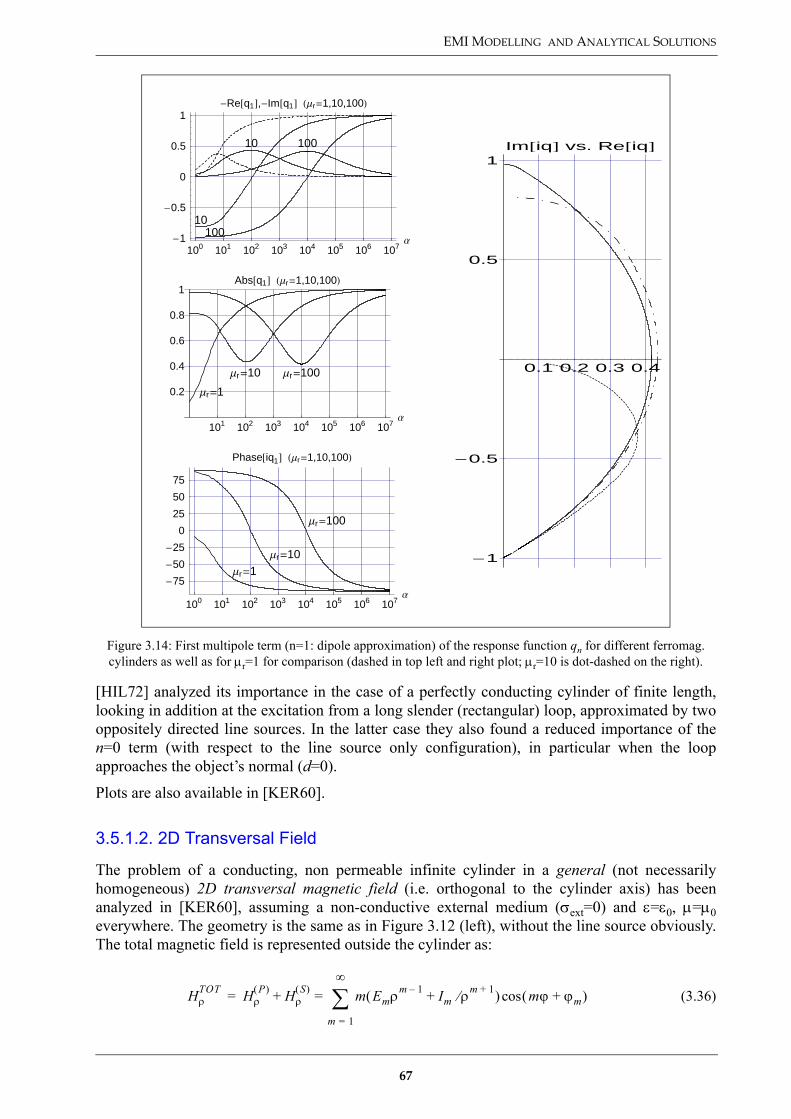
EMI MODELLING AND ANALYTICAL SOLUTIONS
[HIL72] analyzed its importance in the case of a perfectly conducting cylinder of finite length,looking in addition at the excitation from a long slender (rectangular) loop, approximated by twooppositely directed line sources. In the latter case they also found a reduced importance of then=0 term (with respect to the line source only configuration), in particular when the loopapproaches the object’s normal (d=0).
Plots are also available in [KER60].
3.5.1.2. 2D Transversal Field
The problem of a conducting, non permeable infinite cylinder in a general (not necessarilyhomogeneous) 2D transversal magnetic field (i.e. orthogonal to the cylinder axis) has beenanalyzed in [KER60], assuming a non-conductive external medium (σext=0) and ε=ε0, µ=µ0everywhere. The geometry is the same as in Figure 3.12 (left), without the line source obviously.The total magnetic field is represented outside the cylinder as:
(3.36)
Figure 3.14: First multipole term (n=1: dipole approximation) of the response function qn for different ferromag. cylinders as well as for µr=1 for comparison (dashed in top left and right plot; µr=10 is dot-dashed on the right).
100 101 102 103 104 105 106 107Α
�75
�50
�25
0
25
50
75
Phase�iq1� �Μr�1,10,100�
Μr�1Μr�10
Μr�100
101 102 103 104 105 106 107Α
0.2
0.4
0.6
0.8
1Abs�q1� �Μr�1,10,100�
Μr�1
Μr�10 Μr�100
100 101 102 103 104 105 106 107Α�1
�0.5
0
0.5
1�Re�q1�,�Im�q1� �Μr�1,10,100�
10
10
100
100
0.1 0.2 0.3 0.4
�1
�0.5
0.5
1Im�iq� vs. Re�iq�
HρTOT Hρ
P( ) HρS( ) m Emρm 1– Im ρm 1+⁄+( )
m 1=
∞
∑ mϕ ϕm+( )cos=+=
67

CHAPTER 3
(3.37)
The magnetic field corresponding to Em (m=1,2,...) is the primary (or “external”) magnetic field,developed here – in the cylinder’s proximity – in power series (the ρm–1 terms, with coefficientsEm). The magnetic field corresponding to Im is the secondary (or induced, or “internal”) magneticfield, which is a 2m-pole field (see the 1/ρm+1 terms). The relationship between Em and Im (foreach Em an associated Im is given) is obtained by imposing the appropriate boundary conditionson the cylinder’s surface (µr=1 everywhere36), leading to:
(3.38)
Eq. (3.38) has to be compared with the previous result for a line source (Eq. (3.35)), which isindeed a particular case of the 2D transversal field we are considering here. The Em can inprinciple be calculated from the given primary field distribution. Jm are ordinary Bessel functionsof order m.
The m=1 case corresponds again to a homogeneous primary field, the induced field being that ofa 2D dipole (1/ρ2 dependency). It is interesting to note that in this case the induced currents flowalong the z direction (cylinder axis) in one half of the cylinder, and in opposite direction in theother as schematically shown in Figure 3.15, the current circuit closing at infinity. The exactinternal current distribution is calculated in [KER60].
An example is also provided for the case of a 2D dipole, which results in an infinite series ofinduced multipole terms (similarly to the case of a sphere in the field of a 3D dipole). It is pointedout that the induced quadrupole field is usually much smaller than the induced dipole field, giventhe attenuation of the corresponding primary field components at the cylinder, the reducedinduction effect for m=2 with respect to m=1, and the attenuation of the induced quadrupole fieldat the point of observation with respect to the induced dipole field (again similarly to the case of asphere in the field of a 3D dipole). The current and magnetic field distribution inside the cylinderare also calculated.
3.5.1.3. Dipole Source (approximate 3D problem)
[WAI60] has also analyzed the (3D) problem of an infinite circular horizontal cylinder excited byan arbitrarily located magnetic dipolar source, in particular when the source and the receiver arein the equatorial plane. In the latter case an approximate solution is available, at low frequency
36. Actually K=1, similarly to what seen before.
Figure 3.15: Schematic current flow in an infinite cylinder in a transversal magnetic field (for m=1).
HϕTOT Hϕ
P( ) HϕS( ) m Emρm 1– Im ρm 1+⁄–( )
m 1=
∞
∑– mϕ ϕm+( )sin=+=
Im µr 1= a2mJm 1+ iσµω– a( )
Jm 1– i– σµωa( )------------------------------------------Em=
X
Y
X
Y
68

EMI MODELLING AND ANALYTICAL SOLUTIONS
and for a small cylinder (small radius), consisting again of a multipole expansion whose responsefunctions are identical to the qn of the 2D case described above (see Eq. (3.32)). It can also beshown that under the previous assumptions the relative response decreases rapidly withincreasing value of the “mode “number” n. This geometry is also treated in detail in [KAU01,§3.11].
3.5.1.4. Longitudinal Magnetic Field
When the uniform magnetic field is parallel to an infinite horizontal cylinder, ring currents areinduced in it and there is an anomalous internal field distribution; however, if thesecondary fields are null everywhere outside the cylinder [WAR67], [WAR87]. This is obviouslynot the case for a cylinder of finite length.
NdT ApplicationsConcerning NdT applications, the theory of encircling coils and solenoids for tubes and bars(ideally of infinite length – end effects are neglected) is well established [McM86], [LIB71],[VUI94], [BLI97]. In the case of ideal solenoidal coils the primary field is homogeneousthroughout the cross section and confined within the solenoid itself. This setup is not of directpractical application to the scenario we are considering, and is considered separately in A3.2 forthe case of a cylindrical test bar (i.e. a full cylinder). What will be noted here is that the behaviourof the solution for a non-ferromagnetic bar is actually quite similar to the dipole term of a sphere[FOR86b]. The case of ferromagnetic bars is on the other hand quite different, as here the inducedvoltage is simply multiplied by the relative permeability µr (for large µr).
Solutions, expressed in terms of the vector potential, are also available in the case of circularcoaxial (delta-function) coils (single coils, not a solenoid) encircling a coaxial infinite (full)cylinder. These are again reported in A3.2.
3.5.2. (Permeable) Finite Length Cylinders – a Semi-Quantitative ApproachThe previous analytical models have been complemented in a semi-quantitative way in the caseof elongated ferromagnetic objects such as short cylinders, for which demagnetization effects canbe and are relevant.
“Short Parts” in NdTResults for spherical bodies, of practical importance in NdT of short production test parts, havealready been discussed. These exact results can actually be related in a semi-quantitative way[FOR86b] to those for other short production parts, such as cylinders, for which(demagnetization) end effects can become important (see also [STA86]).
Indeed, whereas the case of a non-ferromagnetic sphere approximates the situation of short non-ferromagnetic test objects, important differences do usually arise for ferromagnetic targets. In thelatter case the magnetization is usually not uniform over the object length, decreasing towards theends (in the case of an elongated object whose axis is aligned with the field axis) as a result ofdemagnetization effects37. The latter can be described by a demagnetization factor Nd, whichdepends mainly on the object shape (Nd is not highly dependent on the material’s magneticproperties). In practice the object behaves as if it had an apparent permeability µapp rather than itstrue permeability µr.
37. Certain elliptical shapes, for which the demagnetization field can be made homogenous, represent an exception.
kext2 0≅
69

CHAPTER 3
The Apparent PermeabilityThe complex plane response curves of ferromagnetic objects of different shapes can be describedin semi-quantitative terms by assuming that they behave essentially the same way at the inductivelimit (e.g. for increasing frequency), whereas they strongly depend on the apparent permeabilityat the resistive limit, where magnetization effects dominate. In other words, the response curvesin the complex plane are supposed to maintain a similar shape, starting however from a point(0,µapp–1)38 at the resistive limit which changes according to the object’s shape, size and relativepermeability µr. At the inductive limit they all converge to (0,–1) (compare for example with thecomplex plane plots in Figure 3.11 and Figure 3.14).
In general, the apparent permeability µapp shown by short parts of high permeability (µrel >> µ0)can be written as39:
(3.39)
In the case of an elongated object whose axis is aligned with the field axis the demagnetizationfactor Nd tends to 0 for increasing axial ratios (long axis/short axis), i.e. increasing elongation, inwhich case µapp approaches µrel:
(increasing elongation) (3.40)
In the opposite case of highly permeable (µrel>100 say) but “short” objects (Nd>0.05 say),corresponding to small axial ratios, demagnetization effects are important and the apparentpermeability becomes smaller. Eq. (3.39) simplifies to:
(short, highly permeable parts) (3.41)
In this case Nd dominates. Examples of situations in which this applies include the following:• Sphere: Nd,sph=1/3 and therefore, for high permeability, µapp=3 (as implicitly already obtained in
§3.4.5.2), independent of the actual value of µr!• For short cylinders with length Lcyl and diameter Dcyl, whose axis is parallel to the coil axis, we
have [FOR86b] Nd,cyl=3.4/(4π) for Lcyl/Dcyl=1, which means µapp=3.7, whereas:
for 2<Lcyl/Dcyl<10 (3.42)
again independent of the actual value of µr.• For prolate ellipsoids with fields applied parallel to the long axis and ratios of major (Le) to minor
diameter (De) between 1 and 10, the apparent permeability can be approximated as µapp,ell=3Le/De.This compares favourably with the curves for µ1/µ=100 in [BRA01].
The increase in apparent permeability with increasing object length, actually approaching therelative permeability as described by Eq. (3.40) ( ), can be interpreted in terms of thedemagnetizing influence of the cylinder ends being diminished [FOR86b]. Under this assumptionthe apparent impedance curves tend to approach the curves for an infinitely long, solid cylinderdiscussed in A3.2, and are quite different in the low frequency part from the curves of a sphere orof a cylinder in a transversal magnetic field, for which µapp is basically limited.
38. The –1 term is necessary due to a slight difference in the position of the complex (impedance) plane curves at theinductive limit ((0,0) in NdT, (0,–1) in our case).
39. We have used here SI units following [STA86], rather than [FOR86b]. Eq. (3.39) is basically equivalent to Eq. (7)in [MIL01] apart from the factor –2/3.
1µrel--------- 1
µapp---------- Nd µapp⇒–
µrelNdµrel 1+------------------------- χ
ω 0→lim 1+= = =
Nd 0 µapp µr→⇒→
µapp1
Nd------≅
µappcyl 6
LcylDcyl---------- 5–≅
µapp µr→
70

EMI MODELLING AND ANALYTICAL SOLUTIONS
It is also important to note that in the case of short cylinders with axis perpendicular to the coilaxis, the apparent permeability decreases from 3.7 to 2.0 for Lcyl/Dcyl=1 (because Nd,cyl=1/2),which points to the sensitivity to the object’s orientation in the case of ferromagnetic targets.
Some recent quantitative results are available in [BRA01], whereas [CAR01] provides aninterpretation in terms of natural (resonating) modes, which we will briefly discuss in §3.6.3, andassociates them to dipole and higher order magnetic moments. When reasoning in terms of modesthe variation of the response of a ferromagnetic cylinder with orientation can be interpreted aseither being due to the excitation of a different set of modes, or to changes in the couplingcoefficients, or both.
3.5.3. Finite Length Cylinder in the Field of a Parallel Finite Line SourceAs an example of a configuration which has been solved analytically, and to illustrate theresulting complexity, we will have a look at the problem of a cylinder of electrical properties(σ,µ) and finite length 2s, excited by a symmetrically located axial current filament (also of finitelength, equal to 2l, and traversed by a current I) and embedded in a homogenous medium ofelectrical properties (σ0,µ0). This has been treated in [WAI73b] (see Figure 3.16).
The end conditions are that the total normal current density is zero, which should tend to besatisfied by a thin and highly conducting body. The secondary fields in the plane z=0 are, for ρ>a(a time factor eiωt is used, and omitted as usual):
(3.43)
(3.44)
where the coefficients Λm,n (n=0,1,2,...) replace the qn reflection coefficients (response functions)previously introduced in the case of an infinite cylinder (Eq. (3.32)). In the inductive limit, forexample in the case of a perfectly conducting cylinder, Λm=1. In detail:
Figure 3.16: Geometry for the calculation of the response of a finite length cylinder in the field of a parallel linear current element (adapted from [WAI73b]).
CYLINDER
LINEAR
Z
ρ0
Z
2s
2l
a
CURRENT ELEMENT
Hφs( ) I
π--- Λm n,
n 0=
∞
∑Km unρ0( )Km una( )------------------------Im una( )Km' unρ( )une im φ φ0–( )– λnl( )sin
λns--------------------m ∞–=
∞
∑ , =
Hρs( ) I
πρ------ Λm n,
n 0=
∞
∑m ∞–=
∞
∑Km unρ0( )Km una( )------------------------Im una( )Km unρ( )ime im φ φ0–( )– λnl( )sin
λns--------------------=
71
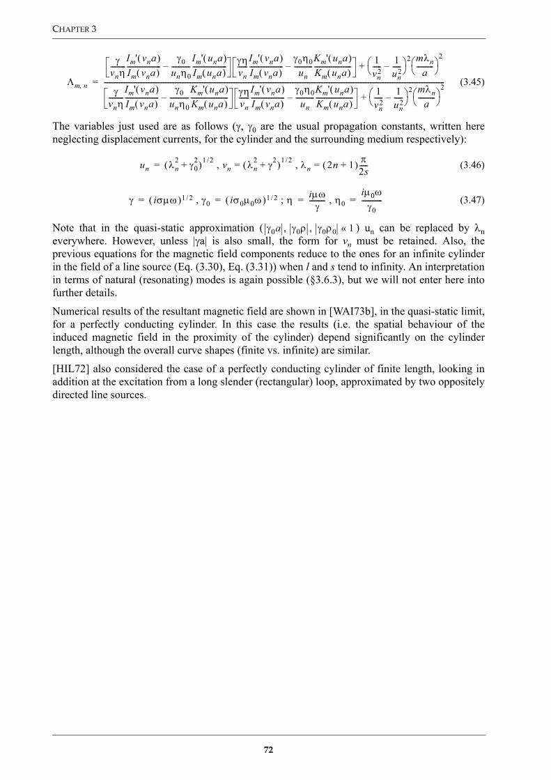
CHAPTER 3
(3.45)
The variables just used are as follows (γ, γ0 are the usual propagation constants, written hereneglecting displacement currents, for the cylinder and the surrounding medium respectively):
(3.46)
(3.47)
Note that in the quasi-static approximation ( ) un can be replaced by λneverywhere. However, unless |γa| is also small, the form for vn must be retained. Also, theprevious equations for the magnetic field components reduce to the ones for an infinite cylinderin the field of a line source (Eq. (3.30), Eq. (3.31)) when l and s tend to infinity. An interpretationin terms of natural (resonating) modes is again possible (§3.6.3), but we will not enter here intofurther details.
Numerical results of the resultant magnetic field are shown in [WAI73b], in the quasi-static limit,for a perfectly conducting cylinder. In this case the results (i.e. the spatial behaviour of theinduced magnetic field in the proximity of the cylinder) depend significantly on the cylinderlength, although the overall curve shapes (finite vs. infinite) are similar.
[HIL72] also considered the case of a perfectly conducting cylinder of finite length, looking inaddition at the excitation from a long slender (rectangular) loop, approximated by two oppositelydirected line sources.
Λm n,
γvnη---------
Im' vna( )Im vna( )--------------------
γ0unη0-----------
Im' una( )Im una( )--------------------– γη
vn------
Im' vna( )Im vna( )--------------------
γ0η0un
-----------Km' una( )Km una( )----------------------– 1
vn2----- 1
un2-----–
2 mλna----------
2
+
γvnη---------
Im' vna( )Im vna( )--------------------
γ0unη0-----------
Km' una( )Km una( )----------------------– γη
vn------
Im' vna( )Im vna( )--------------------
γ0η0un
-----------Km' una( )Km una( )----------------------– 1
vn2----- 1
un2-----–
2 mλna
----------
2+
---------------------------------------------------------------------------------------------------------------------------------------------------------------------------------------------------------=
un λn2 γ0
2+( )1 2/ , vn λn2 γ2+( )1 2/ , λn 2n 1+( ) π
2s-----== =
γ iσµω( )1 2/ , γ0 iσ0µ0ω( )1 2/ ; η iµωγ
--------- , η0iµ0ω
γ0------------= = = =
γ0a , γ0ρ , γ0ρ0 1«
72

EMI MODELLING AND ANALYTICAL SOLUTIONS
3.6. Other Target Models
A number of other models, more specific to UXO/demining applications, have also been devised.They bear partial similarities with what discussed so far, which has been mostly derived in thecontext of geophysical applications. These models will be discussed in the following.
3.6.1. The Induced Dipole ModelFor compact objects sufficiently far from the sensor, the response can be represented in terms ofan induced dipole moment at the target location [BAU98, BEL01a, BEL01b, SOW98a] (the targetis effectively concentrated at a point), which is related in a linear way to the primary field by afrequency-dependent 3×3 magnetic polarizability tensor A(ω). The latter fully characterizes thetarget’s EMI (electromagnetic induction) dipole response, apart from possible nondipole effects;V is the object’s volume. The model assumes a uniform primary field and higher order effects areneglected.
The induced dipole moment m(ω) can therefore be expressed, at a frequency ω, as function of theprimary field HT as (omitting the usual factor exp(iωt)):
(3.48)
The tensor’s elements αjk (j,k=1,2,3) are dimensionless and depend on the target’s electricalproperties, shape and orientation in the primary field, but not on its volume. They are actuallycomplex numbers, reflecting the well known frequency-dependent phase shift between primaryand induced magnetic field. A similar model is also discussed in [WES87] in the context ofgeophysical applications.
For a pulsed sensor (time domain operation) the induced dipole moment m(t) can be expressed asa convolution of the Fourier transform of Vαjk(ω) with the primary field waveform H(t). In termsof components:
(3.49)
The quantity A(t) is in this case an effective polarizability obtained from the convolution of themagnetic polarizability tensor A(ω) with the transmit waveform.
A is symmetric and can therefore be diagonalized by an appropriate rotation of the coordinatesystem:
(3.50)
where U is a transformation matrix between the coordinate system of the sensor and the primaryaxes of the object. The polarizability tensor’s eigenvalues αi(ω) correspond to the responses thatare induced when the primary field is aligned in turn along each of the principal axes of theobject.
In the limit demagnetization effects prevail and the induced dipole moment, and thereforethe product VAHT, must reproduce the static magnetic moment of the object. It can indeed beshown that A(0) can be expressed in terms of the object’s permeability and of its demagnetizationtensor (for details see [BEL01b]).
Note that the dipole model is not synonymous with “simple” spatial behaviour. Indeed, theresponse at any orientation is a linear combination of responses associated with each principalaxis, and the total induced magnetic moment m is therefore not necessarily aligned with HT. Thiscan be clearly seen in the following simplified expression of the induced dipole moment, which isoften used for cylindrical objects:
m VAHT=
mj t( ) V αjk t u–( )Hk u( ) u where α t( )d∫ α ω( ) iωt–( ) ωdexp∫= =
A UΛUT=
ω 0→
73

CHAPTER 3
(3.51)
where L stands for Longitudinal (along the symmetry axis) and T for Transversal (perpendicularto the symmetry axis). This is equivalent to use the following polarizability tensor (diagonalizedform):
(3.52)
This applies also to ordnance items (UXO), which are mostly axisymmetric; two of theeigenvalues are therefore degenerate (in other words, only two eigenvalues are unique). Irregularobjects tend on the other hand to have different responses in three orthogonal directions.
Induced VoltageThe induced dipole moment m can be used to calculate the induced flux through the receivecoil, whose time derivative gives then the induced voltage; the latter is therefore proportional to
[BEL01a].
The voltage induced in the receive coil can also be calculated using reciprocity arguments (see[DAS90, DAS91] for details), leading to the following expression:
(3.53)
where HT is the primary field at the location of the target, and HR is the (hypothetical) incidentfield which would be generated by the receiving coil IF it were used as a transmitter. This type ofapproach is often used to calculate a target’s spatial signature.
Non-dipole EffectsNon-dipole effects can arise due to the fact that real objects have a finite size and that the primaryfields are not uniform (existence of primary field gradients, for example for an elongated objectplaced along the detector’s axis), or because the target response contains higher order multipolecontributions. Examples are provided in [BEL01a].
In typical humanitarian demining scenarios most of the targets are small and probably wellapproximated by the dipole model; non-dipole behaviour is more likely to be due to compositeobjects, made up either of different parts or of separate pieces altogether.
A practical application is likely to have to be coupled to a precise positioning system, and willobviously have to cope with the soil response when this becomes important.
Where all conditions are met the dipole model should however be capable of producinginteresting results, due in particular to the possibility of recovering the target’s response alongeach of its principal axes.
3.6.2. Simple Parametric Response ModelsA number of simple parametric models, more sophisticated than the circuit model presented in§3.1, have been proposed to describe the response of certain targets or target classes. They areusually valid when the primary field is aligned with a principal axis.
A simple generalization of the basic response for spheres and infinite cylinders, which accordingto the authors [BEL01a] does a fairly good job of fitting the EMI spectra of many compact object,especially highly permeable ones, is reported in Eq. (3.54). The model has been synthesized
m mL mT+ αLHL αTHT+= =
AαL 0 00 αT 00 0 αT
=
Φ s( )
m∂– t∂⁄
V s( ) HT A HR⋅ ⋅∝
74

EMI MODELLING AND ANALYTICAL SOLUTIONS
from empirical studies of the EMI response of ordnance and clutter.
(3.54)
The model’s four parameters are an amplitude A, a response time constant τ, a factor c thatdetermines the width of the spectrum, and a factor s that determines the relative magnitude of theasymptotic responses at high and low frequencies. This model is constructed so that it canreproduce the analytical solutions for a wire loop, and for a highly permeable sphere and aninfinite cylinder40. Problems are on the other hand encountered for composite objects, i.e. objectsmade up of two or more distinct parts with different properties (the 20 mm projectile whose datawe will discuss in Chapter 5 represents such a target).
Multiaxis ResponseAs the sensor moves over the target, the latter is in fact illuminated from different directions(different primary field patterns); different combinations of eigenvalues determine therefore themeasured signal, as will be extensively detailed in Chapter 5.
If the measurement positions are accurately known it is however possible to recover thepolarizability tensor (and the target’s position, which is obviously unknown as well), either in thetime or in the frequency domain, by fitting the measured response with the dipole modeldescribed in §3.6.1.
The polarizability tensor can then be diagonalized to obtain its eigenvalues αi(ω) (if working inthe frequency domain), i.e. the response along each of the target’s principal axes41. Theeigenvalue spectra can then be fitted using for example Eq. (3.54) with a different parameter setfor each of the principal axes [BEL01b]. This type of approach – exploiting an object’s EMIspectral signature – has also been termed “EMI Spectroscopy”. It is detailed in [WON01] formines in air at a fixed orientation, and in [NOR01] for UXO using a set of “library spectra” and alinear and non iterative procedure. EMI mine spectra obtained in the laboratory have also beenpreviously discussed by [TRA97], who obtained interesting results for objects with some metalliccontent such as a PMN.
Alternative approach to the exploitation of the eigenvalue distribution are obviously possible, thetarget discrimination capability depending in general on the extent to which the eigenvaluedistributions of target and clutter do not overlap [BEL01a].
3.6.3. Natural (Resonating) ModesThe theoretical justification for the use of simple parametric models similar to Eq. (3.54) is in theprevalence of a few dominant modes [BEL01a] in the target’s response. [BAU98] providesindeed a theoretical basis for modelling EMI responses in terms of poles42 which arecharacteristic of the target, each having a constant (resonant) frequency and an amplitude(excitation strength) which depends on target orientation in the primary field. This is also referredto as the Singularity Expansion Method (SEM) representation, and is not dissimilar to whatdiscussed in §3.3.3, when we looked at the general form of an object’s EM response for largeobjects.
40. A simpler three-parameter model with c=1/2 is actually sufficient in most cases [BEL01b, MIL01].41. In this way we have effectively removed the orientation dependence, if any.42. These poles are situated along the imaginary axis of the complex frequency plane. Such purely imaginary
resonant frequencies do therefore correspond to exponential decays in the time domain systems, having assumedan exp(iωt) time dependency [CAR01].
S ω( ) A s iωτ( )c 2–iωτ( )c 1+
-------------------------+
=
75
CHAPTER 3
[GEN99] discusses in detail these natural modes, or natural resonances, which result in the timedomain in a late-time response characterized by the sum of nearly purely damped exponentials,with the damping constants strongly dependent on target shape, conductivity and permeability.The general concept is specialized to body of revolution (BOR) type objects, comparingmeasurements with data calculated using the theory of cavities or dielectric resonators. [CAR01]extends these results to the response of finite-length cylinders and rings, possibly ferromagnetic;the resulting modes are interpreted in terms of dipole and higher order magnetic moments and asimple and accurate model is provided to compute their resonant frequencies.
It is possible to extract the poles from experimental data, usually a few being sufficient (two orthree maximum), when not just one, to obtain good fitting results, and to attempt targetclassification by matching them against a library of responses. This procedure has also beencalled Magnetic Singularity Identification (MSI). Such an approach has been pursued by anumber of researchers, amongst them [MER99, MER00, RIG01, SOW95, SOW99], and iscritically analysed in [TAN01]. Detailed time-decay data is also shown for a variety of mines in[NEL01], which does not address the classification issue; it does however take into account soileffects, in particular on the response of minimum-metal mines. [MER00] stresses also the pole’ssensitivity to environmental and historical factors, and suggest to put more emphasis on structuralinformation contained in the polarizability tensor, such as symmetries and/or typical ratios ofelements.
Finally, let us point out that the fact of being able to calculate resonant frequencies does obviouslynot mean that the overall target response can be calculated as well (the excitation strengths haveto be known).
76

EMI MODELLING AND ANALYTICAL SOLUTIONS
3.7. A Note on Induction vs. Galvanic Currents
Induction currents correspond to the usual eddy currents (largely confined to the target), whichare generated in direct response to a time-varying magnetic flux cutting across the conductor.
There is however another class of effects which have in principle to be considered inelectromagnetic induction, namely galvanic effects, which are associated with the accumulationof electric charges on the surface43 of conductors (i.e. at their interface). They are included in thesolutions discussed so far, even if we have not mentioned them explicitly.
Galvanic effects do not play a role in some scenarios of common interest, such as in the case ofobjects embedded in an insulating medium (σext=0):
• Sphere in a uniform magnetic field: the radial component of the primary electric field is zero;therefore no electrical charge is formed [KAU01, §3.1].
• Cylinder in a uniform magnetic field perpendicular to the cylinder axis (cylinder elongated in thedirection of the primary electrical field): electrical charges build up on the edges and on thesurfaces near the edges. The influence of edge effects will however decrease progressively withincreasing cylinder length and/or increasing distance of the observation point [KAU01, §3.6].
• Sphere in the field of an arbitrarily oriented magnetic dipole: the primary (vortex) electric fieldEprim (accompanying Hprim) does in general intersect the surface of the conductor, and thereforesurface electrical charges will appear. The basic characteristics of the FD and TD responses(induced magnetic field) are however the same as obtained for the situation with axial symmetry[KAU01, §3.10].
The situation is somewhat more complicated in the case of objects embedded in a conducting full-space (σext>0), for example:
• Cylinder in the field of a parallel line source: as we have seen (§3.5.1.1) the secondary field can beexpressed as a sum of cylindrical harmonics. Those of higher order (n≥1) correspond to the vortexpart of the field, and are generated by currents closed within the cylinder. The fundamental, or n=0component (monopole), corresponds to the galvanic part of the field, and is due to linear currentclosed within the host medium.
• Sphere in the field of an arbitrarily oriented magnetic dipole: Eprim flowlines cross the sphere, andtherefore electrical charges do arise on its surface. Mathematically speaking this translates intosecondary fields expressed in terms of potentials of the electric and magnetic type, correspondingrespectively to TMr and TEr modes (radial Transverse Magnetic and Transverse Electric modes).The source of the second are the “usual” vortex-type induced currents in the target, the source ofthe first is the presence of charges and currents in both the target and host [KAU01, Chapter 6].Under certain conditions a secondary field is produced, which is equivalent to that produced bythe combination of a magnetic and an electric dipole located at the origin of the model.
Conducting Full-Space: Axial Symmetry GeometryThe case of a spheroidal object in the field of a horizontal loop, whose centre is on an object’saxis of symmetry (conductivity σi, radius a) represents a scenario of particular interest for thegeometries we might be confronted with (Axial Symmetry). In this case the normal electricalfield (i.e. the sum of the primary field and of the field generated by currents induced in the hostmedium) does not intersect the surface of the conductor. Therefore no surface electrical chargesappear [KAU01, §5.2], and the only source for the secondary field will be vortex currents.
43. Within each piece of a piece wise uniform medium the volume density of charge is zero [KAU01,§2.5].
77

CHAPTER 3
Axial Symmetry and the Effects of Induced Currents in the Host MediumWe will briefly point out here that for the geometry just discussed (axial symmetry, spheroidalobject), if
(3.55)
the current density in the spheroid will not depend strongly on the conductivity of the externalmedium [KAU01, §5.3], and the secondary fields will therefore be similar to the free space ones.In this case the total scattered fields can be calculated adding the contribution due only to thecurrents in the host medium (no conductor present) to the contribution due only to the currents inthe conductor situated in free space.
This is a priori not guaranteed, i.e. in general the total response is not necessarily equal to the sumof the response of the host medium and of the anomalous conductor taken separately. Theyrespond jointly [NAB91,p.32], similarly to what happens for two closely coupled conductors; forexample, secondary currents can arise in the host medium due to the (induced) currents in thetarget.
The first condition in Eq. (3.55) is practically always satisfied in the scenarios of interest to us(high conductivity contrast), the second, which implies that there is no phase shift in the normalfield (i.e. primary plus host!) within the area occupied by the spheroid, is discussed in more detailin §3.4.2.
Conducting Full-Space: General GeometryFor a general geometry one has in principle to take into account the galvanic part of the secondaryfield as well (also referred to as “channelling”, or “current gathering” – see [SPI84] for a precisedefinition), which is due to the presence of charges and currents that flow in both the target andhost.
The galvanic part is related to the properties of conductors in a different way than the vortex part,and can very well represent the dominant contribution in scenarios of geophysical interest,depending on the type of excitation, the frequency (or time), geometric factors, etc.
[WAL92] reports criteria to estimate the importance of inductive vs. galvanic contributions, for athin vertical plate model, using a vertical magnetic dipole over a half-space. Applied to objects ofinterest to us and at the usual soil conditions and operating frequencies, induction effects shoulddominate for small objects as well as for UXO, with the possible exception of very large objectsin high-conductivity soils. For a standard “blast” mine this should anyhow not be a problem, as itsmetallic parts are mostly isolated from the host medium. Also, the coincident loop configurationdoes apparently minimize galvanic effects [EAT87]. We will therefore not consider galvaniccontributions in the following.
σiσe----- 1 and kea 1«»
78

EMI MODELLING AND ANALYTICAL SOLUTIONS
3.8. Conclusions
A number of analytical solutions to some basic eddy current forward problems of interest to ushave been detailed in this chapter, with emphasis on the analysis of the response function and theoperating conditions prevailing in humanitarian demining. The results for the case of the sphereare for example summarised in §3.4.6 and will not be repeated here.
While analytical solutions can not cover with precision a large number of scenarios, they haverepresented an excellent tool to gain general insight into the physics of the scattering process andits dependence on the model’s parameters. They have been complemented in a semi-quantitativeway for elongated ferromagnetic objects such as short cylinders, for which demagnetizationeffects are important (§3.5.2).
In addition the study of the general form of an object’s EM induction response (§3.3) hasallowed to confirm that these solutions are more general in nature, and to understand how theydepend on the target’s response parameter, and its magnetic permeability in particular. Thegeneral form of the response parameter, which can be obtained via dimensional analysis, isalso noteworthy (§3.3.1).
As has also been stressed by others, e.g. in [SOW95,TRA97,KEI98,WON98,SOW98a,CAR99,SZY99], and in [BRU98a,BRU99b], this theoretical analysis and other similarapproaches indicate the possibility of distinguishing between different objects (e.g.ferromagnetic vs. non-ferromagnetic), and point to the possibility of identifying some metallicobjects based on their characteristic phase response, as already implemented up to a certain levelfor other applications.
In addition, the phase shift of the received signal turns out to be a continuous, monotonicallydecreasing function of the object size44 (all other parameters being kept constant). This leads tothe idea of a coarse classification based on target size (actually the response parameter, see§3.3.1 and §6.3), and/or of discriminating large objects by imposing a “phase threshold”, in orderto reduce the amount of detected clutter when operating in certain scenarios.
This discrimination-based approach is less ambitious than object identification, but should bemore robust, which is of fundamental importance in humanitarian demining tasks, at least forgeneral applications. In fact some think that even a reduction of the false alarm rate of a metaldetector by a factor of 2 or 3 would be highly beneficial, obviously without compromising thedetection efficiency. This approach is likely to work when looking for metallic objects of a certainsize, such as those contained in non minimum-metal mines (e.g. the PMN or PMN2) or UXO, andwhen the clutter is mostly represented by small and/or poorly conductive metallic objects.
The theoretical analysis has also allowed us to identify a few likely problems (§3.3.3), such as thepresence of composite object (§3.3.4) with a potentially complex response function, of elongatedferromagnetic object (§3.5.2), and the fact that the target’s response can well be orientationdependent. Higher order multipole terms (§3.4.4) are on the other hand less likely to represent aproblem in humanitarian demining scenario (they might when larger UXO are present).
Attention has also been drawn to certain second order effects, such as galvanic contributions wellknown in geophysical applications (§3.7); they should in general not be relevant for theapplications of interest to us, with the possible exception of very large objects in high-conductivity soils. For a standard “blast” mine this should anyhow not be a problem, as itsmetallic parts are mostly isolated from the host medium.
44. Concerning applications similar to the one of interest to us, the use of a large phase difference between largemetallic targets such as mines and low-conductivity magnetic nuisance items has already been detailed in[ROS48]. More recently it has been suggested in [BEL94, BAR96] to exploit the phase dependence for thecharacterisation of UXO, to obtain a very rough indication of the object size.
79

CHAPTER 3
We have then briefly investigated the interaction between the target and the host medium in theform of a full space (the response of the host medium by itself will be the subject of Chapter 4). Itis indeed often implicitly assumed that the two decouple (are additive) and this is probably anexcellent approximation in most situations, with the possible exception of high conductivity soilstowards the higher frequency end (see Eq. (3.55)), but strictly speaking it is not guaranteed apriori.
This chapter and the next set the theoretical framework. Experimental results will be thendetailed in Chapter 5 and quantitatively analysed in Chapter 6; they will also be compared withsome of the models’ expectations. Initially unforeseen features will in fact result from the studyof the experimental data, and we will come back when necessary to the models to study theirbehaviour. We will comment on the effectiveness and feasibility of the discrimination-basedapproach at the end of these chapters.
Some of these results have obviously already been known for a certain time, but to the best of ourknowledge not necessarily in this form by those involved with metal detection systems applied tohumanitarian demining needs. We therefore see added value in having put together thisinformation in a coherent way, with emphasis on humanitarian demining specificities, and inhaving moved beyond the simple circuit (§3.1) and sphere approach.
80

EMI MODELLING AND ANALYTICAL SOLUTIONS
Bibliography
[BAR96] B. Barrow, N. Khadr, R. DiMarco, and H. H. Nelson, “The Combined Use of Magnetic andElectromagnetic Sensors for Detection and Characterization of UXO”, Proc. Symposium on theApplication of Geophysics to Engineering and Environmental Problems SAGEEP’96, Keystone,CO, 1996.
[BAU98]C. E. Baum (Ed.), Detection and Identification of Visually Obscured Targets: Taylor & Francis,New York, 1998.
[BEL94] T. Bell, R. DiMarco, and B. Barrow, “UXO Signature Classification and Discrimination”, inProc. Unexploded Ordnance Detection and Range Remediation Conference (May 17-19, 1994,pp. 321-331).
[BEL01a]T. H. Bell, B. J. Barrow, and J. T. Miller, “Subsurface Discrimination Using ElectromagneticInduction Sensors”, IEEE Trans. on Geoscience and Remote Sensing, vol. 39, no. 6, pp. 1286-1293, June 2001.
[BEL01b]T. Bell, B. Barrow, J. Miller, and D. Keiswetter, “Time and Frequency DomainElectromagnetic Induction Signatures of Unexploded Ordnance”, Subsurface SensingTechnologies and Applications, vol. 2, no. 3, pp. 153-175, July 2001.
[BLI97] Blitz, J., 1997, Electrical and Magnetic Methods of Non-destructive Testing: Chapman & Hall,London, UK.
[BRA01] H. Braunisch, C. O. Ao, K. O’Neill, and J. A. Kong, “Magnetoquasistatic Response ofConducting and Permeable Prolate Spheroid Under Axial Excitation”, IEEE Transactions onGeoscience and Remote Sensing, v. 39, no.12, pp. 2689-2701, Dec. 2001
[BRU98a]C. Bruschini, B. Gros, F. Guerne, P.-Y. Pièce, and O. Carmona, “Ground penetrating radar andimaging metal detector for antipersonnel mine detection”, J. of Applied Geophysics 40, pp. 59-71, 1998.
[BRU99b]C. Bruschini, “Metal Detectors for Humanitarian Demining: from Basic Principles to ModernTools and Advanced Developments”, in Proc. MINE’99 (Mine Identification NoveltiesEuroconference), pp. 24-30, Florence, Italy, October 1-3, 1999. Available from http://diwww.epfl.ch/lami/detec/.
[CAR99] L. Carin, I. J. Won, and D. Keiswetter, “Wideband frequency- and time-domain EMI for minedetection”, in SPIE Proceedings Vol. 3710, pp. 14-25, Orlando, FLA, April 1999.
[CAR01] L. Carin, et al., “On the Wideband EMI Response of a Rotationally Symmetric Permeable andConducting Target”, IEEE Trans. on Geoscience and Remote Sensing, vol. 39, no. 6, pp. 1206-1213, June 2001.
[DAS90] Y. Das, J. E. McFee, J. Toews, and G. C. Stuart, “Analysis of an Electromagnetic InductionDetector For Real-Time Location of Buried Objects”, IEEE Trans. on Geoscience and RemoteSensing, vol. 28, no. 3, pp. 278-288, May 1990.
[DAS91] Y. Das, and J. E. McFee, “A Simple Analysis of the Electromagnetic Response of BuriedConducting Objects”, IEEE Trans. on Geoscience and Remote Sensing, vol. 29, no. 2, pp. 342-344, March 1991.
[DOD68]Dodd, C. V., and Deeds, W. E., 1968, Analytical Solutions to Eddy-Current Probe-CoilProblems: Journal of Applied Physics, v. 39, no. 6, May, p. 2829-2838.
[DOD69]Dodd, C. V., Deeds, W. E., and Luquire, J. W., 1969, Integral Solutions to some Eddy CurrentProblems: International Journal of Nondestructive Testing, v. 1, p. 29-90.
[DYA59a]D’Yakonov, B. P., 1959, The diffraction of electromagnetic waves by a circular cylinder in ahomogeneous half-space: (Izv.) Bull. Acad. Sci. U.S.S.R., Geophysics Series, no. 9, 950-955.
[DYA59b]D’Yakonov, B. P., 1959, The diffraction of electromagnetic waves by a sphere located in ahalf-space: (Izv.) Bull. Acad. Sci. U.S.S.R., Geophysics Series, no. 11, 1120-1125.
[EAT87] Eaton, P. A., and Hohmann, G. W., 1987, An evaluation of EM methods in the presence ofgeologic noise: Geophysics, v. 52, p. 1106-1126.
81

CHAPTER 3
[FOR86a]Förster, F., 1986, Theory of encircling coil and internal axial coil tests of tubes: Section 4 in[McM86], p. 89-110; Analysis of encircling coil tests of wire, rods and bars: Section 5 in[McM86], p. 111-145.
[FOR86b]Förster, F., and Wilcox, L.C., 1986, Eddy current tests of spheres and short parts: Section 7 in[McM86], p. 189-204.
[GEN99] N. Geng, C. E. Baum, and L. Carin, “On the Low-Frequency Natural Response of Conductingand Permeable Targets”, IEEE Trans. on Geoscience and Remote Sensing, vol. 37, no. 1, pp.347-359, Jan. 1999.
[GRA65]F. S. Grant and G. F. West, Interpretation Theory in Applied Geophysics. New York: McGraw-Hill, 1965.
[HIL72] Hill, D. A., and Wait, J. R., 1972, Electromagnetic response of a conducting cylinder of finitelength: Geofisica Internacional (Mexico), v. 12, no. 4, October, p. 245-266.
[IDA95] Ida, N., 1995, Numerical Modeling for Electromagnetic Non-Destructive Evaluation: Chapman& Hall, London, UK.
[KAU78]Kaufman, A. A., 1978, Frequency and Transient responses of EM fields created by currents inconfined conductors: Geophysics, v. 43, p. 1002-1010.
[KAU01]A. A. Kaufman, and P. A. Eaton, The Theory of Inductive Prospecting. Amsterdam, NL:Elsevier, 2001.
[KEI98] D. Keiswetter, I. J. Won, T. Bell, B. Barrow, and N. Khadr, “Electromagnetic InductionSpectroscopy”, in Proc. Forum 1998, Anaheim, CA, 5-7 May 1998.
[KEL66] G. V. Keller, and F. C. Frischknecht, Electrical Methods in Geophysical Prospecting. Oxford,UK: Pergamon Press, 1966.
[KER60] Kertz, W., 1960, Leitungsfähiger Zylinder im transversalen magnetischen Wechselfeld(Conducting cylinder in a transversal alternating magnetic field) (in German): GerlandsBeiträge zur Geophysik, v. 69, p. 4-28.
[LIB71] Libby, H. L., 1971, Introduction to Electromagnetic Nondestructive Test Methods: Wiley-Interscience, New York, USA.
[LUQ70] Luquire, J. W., Deeds, W. E., and Dodd, C. V., 1970, Axially Symmetric Eddy Currents in aSpherical Conductor: Journal of Applied Physics, v. 41, no. 10, September, p. 3976-3982.
[McF89] J.E. McFee, “Electromagnetic Remote Sensing; Low Frequency Electromagnetics”, DefenceResearch Establishment Suffield, Ralston, Alberta, Canada, Suffield Special Publication No.124 (report DRES-SP-124), January 1989.
[McM86]McMaster, R. C., McIntire, P., and Mester, M. L. (Eds.), 1986, Nondestructive TestingHandbook, 2nd Edition: Volume 4: Electromagnetic Testing: American Society forNondestructive Testing (ASNT), USA.
[MER99]L. Merlat, M. Acheroy, “Improving quality of information from metal detectors”, in Proc. 1999ARIS Technical Workshop on Ground Survey for Humanitarian Demining, Brest, France, 26-27 Oct. 1999.
[MER00]L. Merlat, and P. Druyts, “Progress Report on the Metal Detector: Signal Processing for TargetDiscrimination and Coil’s Modelization”, Progress Report of the HUDEM Project, RoyalMilitary Academy, Brussels, Belgium, 29 Feb. 2000. Also ISL (Institut de Saint-Louis)Publication PU 322/2000, Saint-Louis, France.
[MIL01] J. T. Miller, T. H. Bell, J. Soukup, and D. Keiswetter, “Simple Phenomenological Models forWideband Frequency-Domain Electromagnetic Induction”, IEEE Trans. on Geoscience andRemote Sensing, vol. 39, no. 6, pp. 1294-1298, June 2001.
[NAB87]Nabighian, M. N. (Ed.), 1987, Electromagnetic Methods in Applied Geophysics, Volume 1,Theory: Investigations in Geophysics No. 3, Society of Exploration Geophysicists (SEG),Tulsa, OK, USA.
[NAB91]Nabighian, M. N. (Ed.), 1991, Electromagnetic Methods in Applied Geophysics, Volume 2,Application: Investigations in Geophysics No. 3, Society of Exploration Geophysicists (SEG),
82

EMI MODELLING AND ANALYTICAL SOLUTIONS
Tulsa, OK, USA.[NEG62] Negi, J. G., 1962, Diffraction of EM waves by an inhomogeneous sphere: Geophysics, v. 27,
Aug., p. 480-492.[NEG63] Negi, J. G., 1963, Discussion on “Diffraction of EM waves by an inhomogeneous sphere”, and
Reply by author: Geophysics, v. 28, p. 665-667.[NEG72] Negi, J. G., Gupta, C. P., and Raval, U., 1972, Induction anomaly due to an elongated covered
ore-zone excited by a long current carrying cable: Geophysical Prospecting, v. 20, p. 193-211.[NEL01] C. V. Nelson, et al., “Wide Bandwidth Time-Domain Electromagnetic Sensor for Metal Target
Classification”, IEEE Trans. on Geoscience and Remote Sensing, vol. 39, no. 6, pp. 1129-1138,June 2001.
[NOR01]S. J. Norton, and I. J. Won, “Identification of Buried Unexploded Ordnance From BroadbandElectromagnetic Induction Data”, IEEE Trans. on Geoscience and Remote Sensing, vol. 39, no.10, pp. 2253-2261, October 2001.
[OGU74]Ogunade, S. O, Ramaswamy, V. and Dosso, H. W., 1974, Electromagnetic Response of aConducting Sphere Buried in a Conducting Earth: Journal of Geomagnetism and Geoelectricity,v. 26, no. 4, p. 417-427.
[OGU80]Ogunade, S. O., and Dosso, H. W., 1980, The Inductive Response of a Horizontal ConductingCylinder Buried in a Uniform Earth for a Uniform Inducing Field: Geophysical Prospecting, v.28, p. 601-609.
[OGU81]Ogunade, S. O., 1981, EM response of an embedded cylinder for line current excitation:Geophysics, v. 46, p. 45-52.
[RIG98] L. S. Riggs, J. E. Mooney, D. E. Lawrence, J. T. Broach, and A. H. Trang, “Identification ofMetallic Mines using Low Frequency Magnetic Fields”, in Detection and RemediationTechnologies for Mines and Minelike Targets III; SPIE Proceedings Vol. 3392 (Orlando, FLA,USA, April 13-17, 1998, pp. 146-157).
[RIG01] L. S. Riggs, J. E. Mooney, and D. E. Lawrence, “Identification of Metallic Mine-Like ObjectsUsing Low Frequency Magnetic Fields”, IEEE Trans. on Geoscience and Remote Sensing, vol.39, no. 1, pp. 56-66, Jan. 2001.
[ROS48] B. Roston, “Development of Locators of Small Metallic Bodies buried in the Ground”, Journalof the Institution of Electrical Engineers (IEE Review), vol. 95, pp. 653-667, 1948.
[SHA] R. S. Sharpe, Ed., “Research techniques in nondestructive testing”, Academic Press, London,1970-1985 (8 vol.).
[SIN73] Singh, S. K., 1973, On Axially Symmetric Electric Current Induced in a Cylinder Under a LineSource: Geophysics, v. 38, no. 5, October, p. 971-974.
[SIN74] Singh, S. K., 1974, Discussion on “Time Dependent Electromagnetic Fields of an Infinite,Conducting Cylinder Excited by a Long Current-Carrying Cable, with reply by author:Geophysics, v. 39, p. 355-356.
[SIN77] Singh, S. K., 1977, Discussion on “Time Dependent Electromagnetic Fields of an Infinite,Conducting Cylinder Excited by a Long Current-Carrying Cable: Geophysics, v. 42, p. 661-662.
[SOW95]Sower G.D., Cave S.P., “Detection and Identification of Mines from Natural Magnetic andElectromagnetic Resonances”, in SPIE Proceedings Vol. 2496, pp. 1015-1024, Orlando, FLA,17-21 Apr. 95.
[SOW98a]G. D. Sower and J. D. Endsley, “The Electrodynamics of Metal Mine Detection”, in Proc.Third Intnl. Symposium on Technology and the Mine Problem, Monterey, CA, April 6-9, 1998.Proceedings on CD-ROM.
[SOW98b]G. D. Sower, “Eddy Current Responses of Canonical Metallic Targets”, in Detection andIdentification of Visually Obscured Targets, C. E. Baum Ed., pp. 243-282, Taylor & Francis,New York, 1998.
[SOW99]G. Sower, J. Endsley, and E. Christy, “Discrimination of Metal Land Mines from Metal Clutter:Results of Field Tests”, in SPIE Proceedings Vol. 3710, pp. 78-88, Orlando, FLA, April 1999.
83

CHAPTER 3
[SPI84] Spies, B. R., and Parker, P. D., 1984, Limitations of large-loop transient electromagneticsurveys in conductive terrain: Geophysics, v. 49, no.7, July, p. 902-912.
[STA86] Stanley, K. R., 1986, Diverted Flux Theory: Section 21 in [McM86], p. 607-630.[SZY99] P. Szyngiera, “A Method of Metal Object Identification by Electromagnetic Means”, in Proc.
MINE’99 (Mine Identification Novelties Euroconference) (Florence, Italy, October 1-3, 1999,pp. 155-160). Available from http://demining.jrc.it/aris/events/mine99/index.htm.
[TAN01] S. L. Tantum, and L. M. Collins, “A Comparison of Algorithms for Subsurface TargetDetection and Identification Using Time-Domain Electromagnetic Induction Data”, IEEETrans. on Geoscience and Remote Sensing, vol. 39, no. 6, pp. 1299-1306, June 2001.
[TRA97] A. H. Trang, P. V. Czipott, and D. H. Waldon, “Characterization of small metallic objects andnon-metallic anti-personnel mines”, in SPIE Proceedings Vol. 3079, pp. 372-383, Orlando,FLA, April 21-24, 1997.
[VEI62] Vein, P. R., 1962, Inductance between Two Loops in the Presence of Solid Conducting Bodies:Journal of Electronics and Control, v. 13, no. 5, p. 471-494. [Probable error in the coefficientfor the sphere, Eq. (62)]
[VUI94] P.-L. Vuillermoz, Les courants de Foucault – Principes, mesure et contrôle, AFNOR, Paris,1994 (in French). ISBN 2-12-260912-5.
[WAI52] Wait, J.R., 1952, The Cylindrical Ore Body in the Presence of a Cable Carrying an OscillatingCurrent: Geophysics, v. 17, April, p. 378-386. [In Eq. (13) replace µ2/µ1 by nµ2/µ1, and in Eq.(14) replace (k+n) by n(k+1) and (k–n) by n(k–1)]
[WAI60] Wait, J.R., 1960, Some Solutions for Electromagnetic Problems Involving Spheroidal, Sphericaland Cylindrical Bodies: Journal of Research of the National Bureau of Standards–B.Mathematics and Mathematical Physics, v. 64B, no. 1, January-March, p. 15-32. [In equation(74) replace ha by |ha|; in equation (80) replace hK'm( ) by |h|K'm( ).]
[WAI73a]Wait, J.R., 1973, On electromagnetic induction in elongated ore bodies (Letters to the Editor):Geophysics, v. 38, no. 5, April, p. 984-985. [Replace “wipe out” by “de-emphasize”]
[WAI73b]Wait, J. R., and Hill, D. A., 1973, Excitation of a homogeneous conductive cylinder of finitelength by a prescribed axial current distribution: Radio Science, v. 8, no. 12, December, p.1169-1173.
[WAI82] Wait, J. R., 1982, Geo-electromagnetism: Academic Press, New York.[WAI97] Wait, J.R., 1997, Belated comments on the electromagnetic cylinder scattering and the
ubiquitous galvanic current distribution (Short Note): Geophysics, v. 62, no. 2, March-April, p.449-450.
[WAL92]Walker, P. W., and West, G. F., 1992, Parametric estimators for current excitation on a thinplate: Geophysics, v. 57, no. 6, June, p. 766-773.
[WAR67]Ward, S. H., 1967, Electromagnetic Theory for Geophysical Applications, in MiningGeophysics, Vol. II, Theory: Society of Exploration Geophysicists (SEG), Tulsa, OK, USA, p.12-196.
[WAR80]Ward, S. H., 1980, Electrical, electromagnetic and magnetotelluric methods: Geophysics, v. 45,no. 11, Nov., p. 1659-1666.
[WAR87]Ward, S. H., and Hohmann, G.W., 1987, Electromagnetic Theory for GeophysicalApplications, in [NAB87], p. 130-311.
[WES91]West, G. F., and Macnae, J. C., 1991, Physics of the Electromagnetic Induction ExplorationMethod, in [NAB91], p. 5-45.
[WON98]I. J. Won and D. Keiswetter, “Electromagnetic Induction Spectroscopy”, in SPIE ProceedingsVol. 3392, pp. 14-22, Orlando, FLA, April 13-17, 1998.
[WON01]I. J. Won, D. A. Keiswetter, and T. H. Bell, “Electromagnetic Induction Spectroscopy forClearing Landmines”, IEEE Trans. Geosci. Remote Sensing, vol. 39, no. 4, pp. 703-709, April2001.
84

EMI MODELLING AND ANALYTICAL SOLUTIONS
Appendix A3.
A3.1. Objects Embedded in a Homogenous Half-Space – Exact SolutionThere are a few geophysical references dealing with the exact analytic solution of the problem ofa conductive and permeable target embedded in a conductive half-space (complications arise dueto the presence of the air-earth interface). We will describe in the following a few of them,without entering in details. Approximate solutions will be sufficient for our aims.
Sphere[NEG62] describes and [NEG63] discusses the diffraction of waves from an inhomogeneoussphere embedded in a half-space, thereby studying the effects of the air-earth boundary, similarlyto the original analysis of [DYA59b]. Primary fields with cylindrical symmetry are considered(e.g. a uniform magnetic field, or a vertical magnetic dipole). The expressions obtained are quiteinvolved. We note in particular the interpretation of part of the response as due to multiplereflections from each of the boundaries. [OGU74] also presents results having mainlygeophysical interest.
Cylinder[DYA59b] obtained an exact analytical solution to the problem of a conducting cylinder buried ina uniform earth as a limiting case of the boundary value problem involving two non-concentriccylinders. [OGU81] treats an extension to this solution for an infinite horizontal cylinder in thefield of a line source. The actual numerical results are not of particular interest for us.
A3.2. Infinite Cylinder in a Longitudinal Magnetic Field – NdT
Solenoidal CoilsConsidering the case of a cylindrical test bar (i.e. a full cylinder) of diameter dbar, the totalvoltage Vsec/V0 induced in a secondary (receiving) solenoidal coil of diameter Dcoil, normalizedby the empty coil voltage V0, or equivalently the impedance Z=((R–R0)/ωL0, ωL/ωL0) in case asingle coil is used, normalized by ωL0, is [FOR86a]:
(A3.1)
(A3.2)
where L0 and R0 are the self-inductance and the resistance of the empty encircling coil, η=(dbar/Dcoil)2 is the coil fill factor and J0 and J1 are Bessel functions of the zero and first orderrespectively. The effective permeability µeff plays here the role of response function, with thefrequency ratio f/fg used in NdT being nothing else than the response parameter (ka)2=σµωa2.Note that sec refers here to the coil, not the voltage.
It is quite interesting to note that the behaviour of the solution for a non-ferromagnetic bar isactually quite similar to the dipole term of a sphere [FOR86b], as shown in Figure 3.17 (smalldashed curve). The case of ferromagnetic bars is on the other hand quite different, as here theinduced voltage is simply multiplied by the relative permeability µr (for large µr) – see the dot-dashed (µr=2) and continuous curve (µr=5) again in Figure 3.17.
Vimagsec
V0------------- ωL
ωL0---------- 1 η η+– µrelµeff real( ) ,
Vrealsec
V0-----------
R R0–ωL0
--------------- ηµrelµeff imag( )= == =
µeff2
f fg⁄---------–
J1 if fg⁄( )
J0 if fg⁄( )-------------------------- 1 i–( )=
85

CHAPTER 3
Circular (delta-function) CoilsSolutions, expressed in terms of the vector potential, are also available in the case of circularcoaxial (delta-function) coils (single coils, not a solenoid) encircling a coaxial infinite (full)cylinder of radius b (see Figure 3.18).
If coil "1", of radius a1 and placed at z=0, is the exciting coil, the general expression for themagnetic vector potential A(ρ,z) outside the cylinder is (A1' is valid for b ≤ ρ ≤ a1, A1'' for ρ ≥ a1;A1 will not be considered here) [VEI62]:
(A3.3)
(A3.4)
The first term is due to the exciting coil itself (primary field), the second one corresponds to thedisturbance introduced by the cylinder. The Dλ coefficient is (W2=λ2–k2, where k is the usualpropagation constant):
Figure 3.17: Response of a full infinite cylinder in a longitudinal field (generated by a solenoid) for η=1. Dashed: µr=1, dot-dashed: µr=2, continuous: µr=5.
Figure 3.18: Circular coaxial coils encircling an infinite cylinder
0.5 1 1.5
1
2
3
4
5�ΜrelIm�iΜeff� vs. ΜrelRe�iΜeff�
Μr�5
Μr�2
Μr�1
C1
bCYLINDER
Z
A1'A1''
a1
A1
a2
C2
A1'µ0a1I1
π---------------- K1 λa1( ) I1 λρ( ) DλK1 λρ( )+[ ] λz λdcos
0
∞
∫=
A1''µ0a1I1
π---------------- K1 λρ( ) I1 λa1( ) DλK1 λa1( )+[ ] λz λdcos
0
∞
∫=
86

EMI MODELLING AND ANALYTICAL SOLUTIONS
(A3.5)
When a single coil is used, or two coincident coils, we can replace ρ=a1=a and z=0 in Eq. (A3.3)or Eq. (A3.4) and obtain for the total induced voltage:
(A3.6)
(A3.7)
where the first term in the integral corresponds to the coil self-inductance L and contains alogarithmic singularity (as we are considering delta-function coils, i.e. of infinitesimal crosssection). [DOD68], [DOD69] extend these results to coils of finite cross section encircling twoconcentric cylinders (which contains the special case of hollow cylinders).
A3.3. Special FunctionsThe associated Legendre polynomials are defined as (n, m integer):
(A3.8)
where Pn(x) is an ordinary Legendre polynomial of order n. We have in particular:
(A3.9)
Note that some authors prefer to omit the (–1)m factor.
Concerning the modified Bessel functions of the first kind, we have in particular that:
(A3.10)
DλλµrI1 Wb( )I0 λb( ) WI0 Wb( )I1 λb( )–
λµrI1 Wb( )K0 λb( ) WI0 Wb( )K1 λb( )+----------------------------------------------------------------------------------------------=
V jω A ld⋅∫° jω= 2πaA z 0=ρ a= …= =
… jω2µ0a2I1 K1 λa( ) I1 λa( ) DλK1 λa( )+[ ] λd0
∞
∫ jωLI1 2µ0a2I1 Dλ K1 λa( )[ ]2 λd0
∞
∫+= =
Pnm x( ) 1–( )m 1 x2–( )
m 2⁄
xm
m
dd Pn x( )=
P11 x( ) 1 x2– , P2
1 x( ) 3x 1 x2– , P31 x( ) 3
2--- 1 x2– 1– 5x2+( )–=–=–=
I 1– 2⁄ z( ) 2πz----- z( ) , I1 2⁄ z( ) 2
πz----- z( ) , I3 2⁄ z( ) 2 z( ) 2 z( )sinh z⁄–cosh2πz
--------------------------------------------------------=sinh=cosh=
87

CHAPTER 3
88

4. Electromagnetic Induction Ground Response
The presence and importance of the soil signal for Frequency Domain systems havealready been stressed in Chapters 1 and 2 (§2.2.4, §2.3.1 and §2.3.3.2 in particular). Itis therefore important to gain a quantitative understanding of the role of thedifferent parameters – the soil’s EM properties, the metal detector’s loop size andheight – and of some techniques, such as frequency differencing methods, which areused to reduce soil effects. This will also help in understanding the behaviour of theexperimental data in Chapter 5 and in the analysis of features more robust tobackground fluctuations (Chapter 6).
The response of the earth itself can be calculated using known results for theresponse of a (homogenous) half-space in Geophysics, or equivalently from a semi-infinite medium in NdT, although this might at first glance look astounding giventhe usually very different target scenarios involved (the range of conductivity valuesis very different in general – say of maximum 1 S/m in Geophysics vs. theconductivity of metals in the case of NdT). What is certainly different is the relativemagnetic permeability of the half-space, which is usually very close to 1 for the soil,whereas it can assume very large values for a permeable metallic substrate.
In the following we will consider the response to a loop of finite size, leaving asidethe large body of literature dealing with the dipole (“small loop”) approximation.We will also be interested in the induced voltage rather than in the magnetic field;the latter can actually be expressed analytically for example at the centre of the loop,whereas all other quantities are available only in integral form in the general case.
Note that in geophysical articles the z-axis points often downwards, i.e. positive z isin the direction of the half-space, in NdT usually upwards; also, the origin issometimes taken at the coil rather than at the surface.
4.1. Loop Response in Geophysics
Concerning geophysical applications, one of the earliest papers dealing with the problem of a(delta-function) horizontal circular loop above a horizontally layered half-space was [MOR69],specializing the solution to the total electric and magnetic fields in integral form at the surface.The harmonic fields are then used, as is often the case, to calculate transient quantities (a half sinewave current pulse in this case). This work is further developed in [RYU70], which overcomesthe impracticality of numerical evaluation of the previously found solution when the loop is on orclose to the surface (h~0) (severe oscillation of the integrand when the total fields are calculated,rather than the secondary only, in which we are interested). Solutions are obtained in particularfor the fields outside and in the centre of the loop. The voltage induced in the loop, rather than thefields, was calculated in [LEE74], making use of the expression for the induced electric field atthe loop itself. The result is then again used to calculate transient quantities.
The permeability of the ground is often assumed to be equal to unity in a number of geophysicalpapers. An exception is for example [IGN85], which starts by calculating the electric field in thefrequency domain in terms of an appropriate Green’s function. The total electric field is expressedas a sum of a “radiative” and evanescent and a “diffusive” and dissipative partial field; althoughthe form is different, the expressions thus obtained are equivalent to Eq. (4.7) and Eq. (4.8). Thesolution is then inverted to the time domain (step current excitation) and the effects of changes inthe permeability contrast and in the loop height are analyzed.
Finally, a number of results for rectangular and circular loops are also reviewed in [WAR87].
89
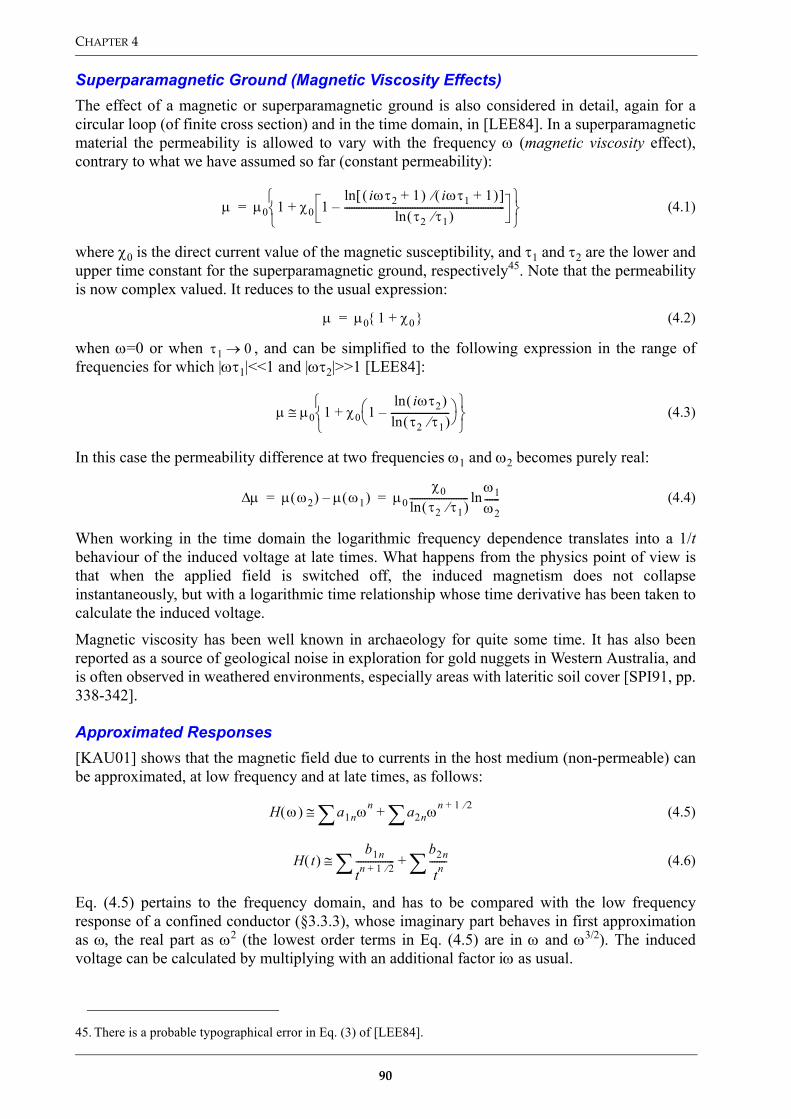
CHAPTER 4
Superparamagnetic Ground (Magnetic Viscosity Effects)The effect of a magnetic or superparamagnetic ground is also considered in detail, again for acircular loop (of finite cross section) and in the time domain, in [LEE84]. In a superparamagneticmaterial the permeability is allowed to vary with the frequency ω (magnetic viscosity effect),contrary to what we have assumed so far (constant permeability):
(4.1)
where χ0 is the direct current value of the magnetic susceptibility, and τ1 and τ2 are the lower andupper time constant for the superparamagnetic ground, respectively45. Note that the permeabilityis now complex valued. It reduces to the usual expression:
(4.2)
when ω=0 or when , and can be simplified to the following expression in the range offrequencies for which |ωτ1|<<1 and |ωτ2|>>1 [LEE84]:
(4.3)
In this case the permeability difference at two frequencies ω1 and ω2 becomes purely real:
(4.4)
When working in the time domain the logarithmic frequency dependence translates into a 1/tbehaviour of the induced voltage at late times. What happens from the physics point of view isthat when the applied field is switched off, the induced magnetism does not collapseinstantaneously, but with a logarithmic time relationship whose time derivative has been taken tocalculate the induced voltage.
Magnetic viscosity has been well known in archaeology for quite some time. It has also beenreported as a source of geological noise in exploration for gold nuggets in Western Australia, andis often observed in weathered environments, especially areas with lateritic soil cover [SPI91, pp.338-342].
Approximated Responses[KAU01] shows that the magnetic field due to currents in the host medium (non-permeable) canbe approximated, at low frequency and at late times, as follows:
(4.5)
(4.6)
Eq. (4.5) pertains to the frequency domain, and has to be compared with the low frequencyresponse of a confined conductor (§3.3.3), whose imaginary part behaves in first approximationas ω, the real part as ω2 (the lowest order terms in Eq. (4.5) are in ω and ω3/2). The inducedvoltage can be calculated by multiplying with an additional factor iω as usual.
45. There is a probable typographical error in Eq. (3) of [LEE84].
µ µ0 1 χ0 1iωτ2 1+( ) iωτ1 1+( )⁄[ ]ln
τ2 τ1⁄( )ln------------------------------------------------------------------–+
=
µ µ0 1 χ0+{ }=
τ1 0→
µ µ0 1 χ0 1iωτ2( )lnτ2 τ1⁄( )ln------------------------–
+
≅
µ∆ µ ω2( ) µ ω1( )– µ0χ0τ2 τ1⁄( )ln------------------------
ω1ω2------ln= =
H ω( ) a1nωn a2nωn 1 2⁄+∑+∑≅
H t( )b1n
tn 1 2⁄+----------------b2n
tn-------∑+∑≅
90

EMI GROUND RESPONSE
Eq. (4.6) is relative to the time domain; the induced voltage is the time derivative thereof, andfeatures therefore an additional factor 1/t. The currents induced in the host medium decreaseduring the late stage much more slowly (as t–3/2) than those of a confined conductor, whose latetime response decays exponentially. It can therefore be problematic to measure small signalsaccurately. On the other hand one can in principle choose an optimum measurement range wherethe target signal is strongest relatively to the host medium response. The same argument isactually valid in the frequency domain (existence of an “optimum frequency range”).
4.2. Loop Response in NdT
We will use as reference the result quoted in [CHE65], which is quite general. Considering avanishingly thin (delta-function), circular coil of radius a in air, with axis oriented along the z axis(pointing upwards) and placed at z=h of the cylindrical coordinate system (ρ,φ,z), in theproximity of a semi-infinite medium (half-space) of electrical parameters (ε1,σ,µ1) occupying theregion z<0 (see Figure 4.1), the total magnetic vector potential Aφ can be expressed in integralform as follows in air (z>0) and in the medium (z<0) respectively:
(4.7)
(4.8)
where J1 is the Bessel function (of the first kind) of the first order, and k0 and k1 are respectivelythe propagation constants in air and in the medium:
(4.9)
The previous expression for Aφ are complete (not quasi-static).
The factor in braces in Eq. (4.7) can be interpreted as a reflection coefficient, and [CHE65] showsthat it corresponds indeed to the reflection coefficient rTE in air of horizontally polarized planewaves (TE or Transverse Electric mode), into which the spherical waves involved in this problemcan be expanded. Additional elements can be found in [WAR87].
Starting from the vector potential a number of physical quantities characteristic of inductionphenomena can again be calculated, in particular the voltage induced in a second coil coincidentwith the one just considered, or in the coil itself [DOD68, DOD69]. Indeed, letting z=h and ρ=ain Eq. (4.7) we obtain for the total induced voltage VTOT:
Figure 4.1: Circular loop above a homogenous medium (soil)
AIR
Z=0
a
SOILσ, µ1, ε1
X
Z
Y
h
ρφ
I(ω)
Aφ z 0>
µ0Ia2----------- J1 ξρ( )J1 ξa( )e
λ0 z h–– ξ ξdλ0
---------µ0Ia
2----------- J1 ξρ( )J1 ξa( )eλ0 z h+( )– µ1λ0 µ0λ1–
µ1λ0 µ0λ1+------------------------------ ξ ξd
λ0---------
0
∞
∫+0
∞
∫=
Aφ z 0<
µ0Ia2----------- J1 ξρ( )J1 ξa( )e
λ1z λ0h– 2µ1ξ ξdµ1λ0 µ0λ1+------------------------------
0
∞
∫=
λ0 ξ2 k02– , λ1 ξ2 k1
2–== with k02 ε0µ0ω2= , k1
2 ε1µ1ω2 i– σµ1ω=
91

CHAPTER 4
(4.10)
(4.11)
The first term within brackets corresponds to the coil voltage induced by the primary field in theabsence of the infinite medium, and is actually logarithmically singular corresponding to aninfinite coil self-impedance L due to the assumption of delta-function coil, as already seen inA3.2. This would not happen for a coil of finite cross section. The second term is regular andcorresponds to the secondary voltage, for which there are some numerical convergence problemsfor h~0 and µ1>µ0 due to strong oscillations of the Bessel function; they are however damped bythe exponential when the coil is lifted from the ground (h>0). There is also a singularity due to λ0,with which we will in fact not be confronted (see the approximations below).
[CHE65] shows a number of plots for conductivity values of interest in NdT (“metallic” values),which are, as we said, much higher than those of typical interest in Geophysics.
It is actually of interest to introduce (adimensional) quantities normalized in terms of the coilradius a. This is achieved by dividing the height by a and multiplying λ0, λ1 and ξ by a, resultingin (the quantity within braces is now adimensional as well):
(4.12)
(4.13)
with
(4.14)
(4.15)
Whereas Eq. (4.12) is again exact, in Eq. (4.14) approximated expressions for λ0N and λ1N havebeen obtained neglecting displacement currents in both the air and the ground (quasi-staticapproximation). χHS is the half-space response function which will be plotted in the following,using α, the usual adimensional response parameter (induction number) which depends here onthe coil radius a, as plotting variable. Note that the height hN is normalized by the coil radius. Theinduced voltage can be obtained by multiplying the response function values with thenormalization factor iωµ0πIa; the latter depends in particular on ω.
Note that we are interested in quite low values of α, with maximum of about 10–3-10–2 say for atypical metal detector of radius 10-15 cm in a high conductivity soil at a frequency of 100 kHz(see also Table 3.2). In the case of large loops – radius of order 1 m – αmax could be of the order of1-10.
More complex scenarios than the uniform half-space have been studied as well, although resultsare often specialized to non-permeable media, such as multiple (metallic) layers. [DOD68,DOD69] detail the solutions for a two-layer planar conductor and also extend the results to coilsof finite cross section and to a number of physical quantities of interest. It can be shown that thepreviously quoted results are a special case of the more general ones. The geophysical analogue isa stratified ground (layered earth models), which has been discussed in some of the previouslymentioned references as well as in [WAI82]. Concerning more recent NdT literature, analytical
VTOT iωa Aφ z h=
ρ a= φd
π–
π
∫ iω2πaAφ z h=
ρ a= …= = =
… iωµ0πIa2 J1 ξa( )[ ]2ξ ξdλ0
--------- J1 ξa( )[ ]2e2hλ0– µ1λ0 µ0λ1–
µ1λ0 µ0λ1+------------------------------ ξ ξd
λ0---------
0
∞
∫+0
∞
∫
VPRIM VSEC+= =
VTOT iωµ0πIa J1 x( )[ ]2x xdλ1N-------- J1 x( )[ ]2e
2hNλ0N– µ1λ0N µ0λ1N–µ1λ0N µ0λ1N+------------------------------------
x xd
λ0N--------
0
∞
∫+0
∞
∫
…= =
… VPRIM iωµ0πIa( )χHS+=
hN h a⁄= , λ0N aλ0 aξ≅ x , λ1N aλ1 a2ξ2 iσµ1ωa2+≅= x2 iα+= = =
x aξ , α σµ1ωa2= =
92

EMI GROUND RESPONSE
and numerical results are also discussed in [OAT92, BLI97]46. Linear, isotropic andhomogeneous media are usually assumed throughout.
Further comments can be found in the interesting overview of EM methods in NdT of wire ropesby Wait [WAI79], which includes a summary of papers dealing with the basic concepts andtechniques for testing of cylindrical conductors by both electric and magnetic methods, andrecalls the extensive related work on electromagnetic probing of geophysical targets.
In the following we will analyse the half-space response function for a number of scenarios ofinterest.
4.2.1. Non-Magnetic Ground (µr=1)The response function for a non-magnetic ground with the loop on the ground (hN=0) is plotted inFigure 4.2, and resembles the one for a non-ferromagnetic sphere. Our interest is here howevertowards much lower values of the response parameter.
The imaginary component (continuous line) is a straight line with slope equal to one, whichmeans linear dependence on α and therefore on ω in particular; the real component (dashed line)has slope 3/2, implying dependence on α3/2 and therefore on ω3/2. The phase does not exceed afew degrees for a typical metal detector, as in this case the real part is several orders of magnitudesmaller than the imaginary one47.
From the numerical point of view there is practically no difference in this case between usinghN=0 or hN=0.01 (see below). Also, an upper integration limit of 10 was sufficient for the secondintegral in Eq. (4.12) when µr=1. The results coincide with those obtained from Eq. 5.50 in[KAU01], apart from a factor π.
46. Both publications refer to an error in the original differential equation for the vector potential by Dodd and Deeds[DOD68], which we have however not been able to identify (the corresp. equation seems dimensionally correct).
Figure 4.2: Half-space response function for a non-magnetic soil (µr=1) and hN=0 (loop on the ground). Top: –Re is dashed, –Im continuous. Bottom left: phase, bottom right: complex plane.
47. Note that the phase of iχHS is plotted, to obtain directly the phase of the induced voltage.
10�110�210�310�4 100 101Α
�40
�30
�20
�10
0Phase�iΧHS� �Μr�1,h�0�
0.05 0.1 0.15
�0.2
�0.15
�0.1
�0.05
Im�iΧHS� vs. Re�iΧHS�
Α�1
Α�10
10�110�210�310�4 100 101Α0
0.05
0.1
0.15
0.2
�Re�ΧHS�,�Im�ΧHS� �Μr�1,h�0�
10�110�210�310�410�510�6 100 101Α
10�1
10�2
10�3
10�4
10�5
10�6
10�7
10�8
10�9
10�10
�Re�ΧHS�,�Im�ΧHS� �Μr�1,h�0�
93

CHAPTER 4
The results for a loop on and above the ground are shown in Figure 4.3 (–Phase is plotted here).For a 10 cm radius loop, for example, the case hN=0.1 corresponds to an absolute height of 1 cm,hN=1 to 10 cm. Note the decrease in amplitude with height, more marked for the imaginarycomponent.
4.2.2. Magnetic Ground (µr>1)
The response function for a para- or weakly ferromagnetic ground with the loop very close to theground (hN=0.01) is plotted in Figure 4.4, and resembles the one for a ferromagnetic sphere. Ourinterest goes however again to much lower values of the response parameter.
The real part of the response function, whose absolute value is plotted, decreases at decreasing α,becomes negative (values to the left of the dip in the logarithmic scale) and reaches a plateau dueto induced magnetization effects. When working in this region the real part of the response isbasically frequency- and conductivity independent and represents therefore a constant shift withrespect to the value for µr=1. Under these conditions the real part can be much larger than theimaginary one, which translates into values of the phase response very close to +90°. Theimaginary part of the response function is basically unaffected by permeability changes.
It can also be shown that the constant plateau value thus reached is proportional to thepermeability for small values of µr, up to about 1.5. Indeed, in the case of a loop on a half-spacethe vertical component of the magnetic field at the centre of a loop varies at low frequencies withthe ground’s magnetic susceptibility κ as [THO77]:
(4.16)
which is in first approximation proportional to ∆κ for small susceptibility values.
From the numerical point of view the integration at hN=0 is somewhat impractical; we havetherefore chosen to use hN=0.01. Also, the upper integration limit was extended to 100 in thesecond integral in Eq. (4.12).
The results for a loop very close to and above the ground are shown in Figure 4.5. Note thedecrease in amplitude with height, more marked here for the real component (the uppermostcurves correspond to hN=0.01, the lowermost ones to hN=1), whose zero crossing position (dip inthe Log scale) moves towards lower values of α. As the imaginary part is not much affected bythe permeability, the resulting phase is quite influenced by height changes, in particular for lowervalues of µr. The bottom right plot covers the low α region, where the phase is very close to +90°.
Figure 4.3: Half-space response function for a non-magnetic soil (µr=1) as a function of loop height: hN=0 (black), hN=0.1 (blue) and hN=1 (red, dot-dashed on the right). Left: –Re is dashed, –Im continuous.
10�110�210�310�410�510�6 100 101Α
10�1
10�2
10�3
10�4
10�5
10�6
10�7
10�8
10�9
10�10
�Re�ΧHS�,�Im�ΧHS� �Μr�1; h�0,0.1,1�
�Im�Re
10110010�110�210�310�410�5Α
0.1
1
10
100�Phase�iΧHS� �Μr�1; h�0,0.1,1�
h�0
h�1
Hz∆Hz
--------- κ∆1 κ+( ) 2 κ+( )
----------------------------------- where µ 1 κ+( )µ0= =
94
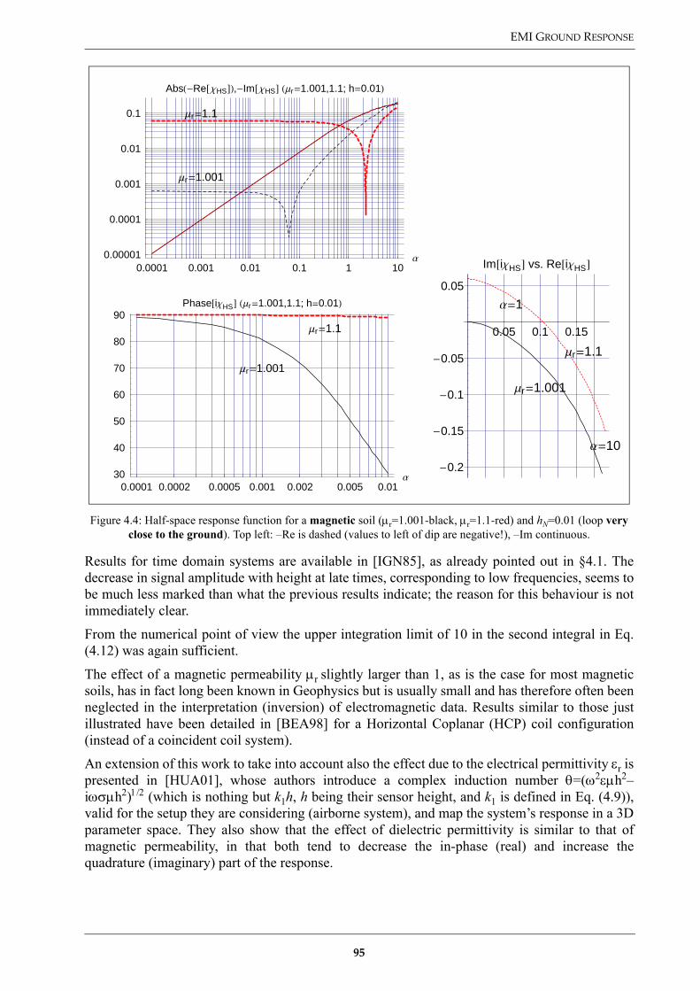
EMI GROUND RESPONSE
Results for time domain systems are available in [IGN85], as already pointed out in §4.1. Thedecrease in signal amplitude with height at late times, corresponding to low frequencies, seems tobe much less marked than what the previous results indicate; the reason for this behaviour is notimmediately clear.
From the numerical point of view the upper integration limit of 10 in the second integral in Eq.(4.12) was again sufficient.
The effect of a magnetic permeability µr slightly larger than 1, as is the case for most magneticsoils, has in fact long been known in Geophysics but is usually small and has therefore often beenneglected in the interpretation (inversion) of electromagnetic data. Results similar to those justillustrated have been detailed in [BEA98] for a Horizontal Coplanar (HCP) coil configuration(instead of a coincident coil system).
An extension of this work to take into account also the effect due to the electrical permittivity εr ispresented in [HUA01], whose authors introduce a complex induction number θ=(ω2εµh2–iωσµh2)1/2 (which is nothing but k1h, h being their sensor height, and k1 is defined in Eq. (4.9)),valid for the setup they are considering (airborne system), and map the system’s response in a 3Dparameter space. They also show that the effect of dielectric permittivity is similar to that ofmagnetic permeability, in that both tend to decrease the in-phase (real) and increase thequadrature (imaginary) part of the response.
Figure 4.4: Half-space response function for a magnetic soil (µr=1.001-black, µr=1.1-red) and hN=0.01 (loop very close to the ground). Top left: –Re is dashed (values to left of dip are negative!), –Im continuous.
0.0001 0.0002 0.0005 0.001 0.002 0.005 0.01Α30
40
50
60
70
80
90Phase�iΧHS� �Μr�1.001,1.1; h�0.01�
Μr�1.001
Μr�1.1
0.0001 0.001 0.01 0.1 1 10Α0.00001
0.0001
0.001
0.01
0.1
Abs��Re�ΧHS��,�Im�ΧHS� �Μr�1.001,1.1; h�0.01�
Μr�1.001
Μr�1.1
0.05 0.1 0.15
�0.2
�0.15
�0.1
�0.05
0.05
Im�iΧHS� vs. Re�iΧHS�
Α�1
Α�10
Μr�1.001
Μr�1.1
95

CHAPTER 4
We have on the other hand chosen to ignore displacement currents, as already discussed, whichleads to a simpler response parameter of the well known iωσµa2 form where a is here the coilradius, see Eq. (4.14) and Eq. (4.15). This is a good approximation, in our scenario, when notworking at high frequencies, say less than 100 kHz, and in not excessively resistive ground, i.e.when displacement currents can be prevalent, as already discussed in §3.4.2.
4.3. Frequency Differencing Methods
The possibility of reducing the background signal due to the soil, in order to enhance the signal tonoise ratio, has been recognized quite a long time ago. One of the possible techniques whenworking with frequency domain systems foresees the use of two or more different frequencies.[WAR67] does already mention the use of multiple frequency operations to reduce terrain noise,whereas [KEL66] describes the use of difference signals for background rejection. Frequencydifferencing methods are also well known in Non-Destructive Testing, e.g. to reduce thebackground response due to interfering (fixed) objects.
The basic idea is that the difference signal(s) is/are null when no target object is present, whereasin presence of a conductive zone the mutual coupling between the transmitter and the receivercoil changes (more at the higher than at the lower frequency) and an anomaly is recorded in thedifference channel(s). Multigeometry systems have also been described as well in the geophysicalliterature.
There are actually several different ways of combining a detector’s output at different frequenciesto generate difference signals, and their degree of effectiveness depends in general on the natureof the background, on the type of the target and on the operating conditions (system frequencyand geometry, which influence the background and target response parameters). [KAU89]discusses a few of them for several geophysical scenarios, and compares the results to thoseachievable with time domain methods.
Figure 4.5: Half-space response function for a magnetic soil as a function of loop height. Top row: left: µr=1.001, right: µr=1.1, and hN=0.01 (uppermost curves), hN=0.1 and hN=1 (lowermost curves); –Re is dashed (values to left of
dip are negative!), –Im continuous. Bottom row: hN=0.01 (continuous), hN=0.1 (dashed) and hN=1 (dot-dashed).
10�110�210�310�4 100 101Α
10�1
10�2
10�3
10�4
10�5
10�6
Abs��Re�ΧHS��,�Im�ΧHS� �h�0.01,0.1,1�
�Im
��Re� Μr�1.001
10�110�210�310�4 100 101Α
10�1
10�2
10�3
10�4
10�5
Abs��Re�ΧHS��,�Im�ΧHS� �h�0.01,0.1,1�
�Im
��Re�
Μr�1.1
1.�10�6 0.00001 0.0001 0.001 0.01Α
0
20
40
60
80
Phase�iΧHS� �Μr�1.001,1.1; h�0.01,0.1,1�
Μr�1.001
Μr�1.1
h�1
h�0.1
h�0.0
10�8 10�7 10�6 10�5Α
89.2
89.4
89.6
89.8
90Phase�iΧHS� �Μr�1.001,1.1; h�0.1,1�
Μr�1.1
h�0.1
h�1
96
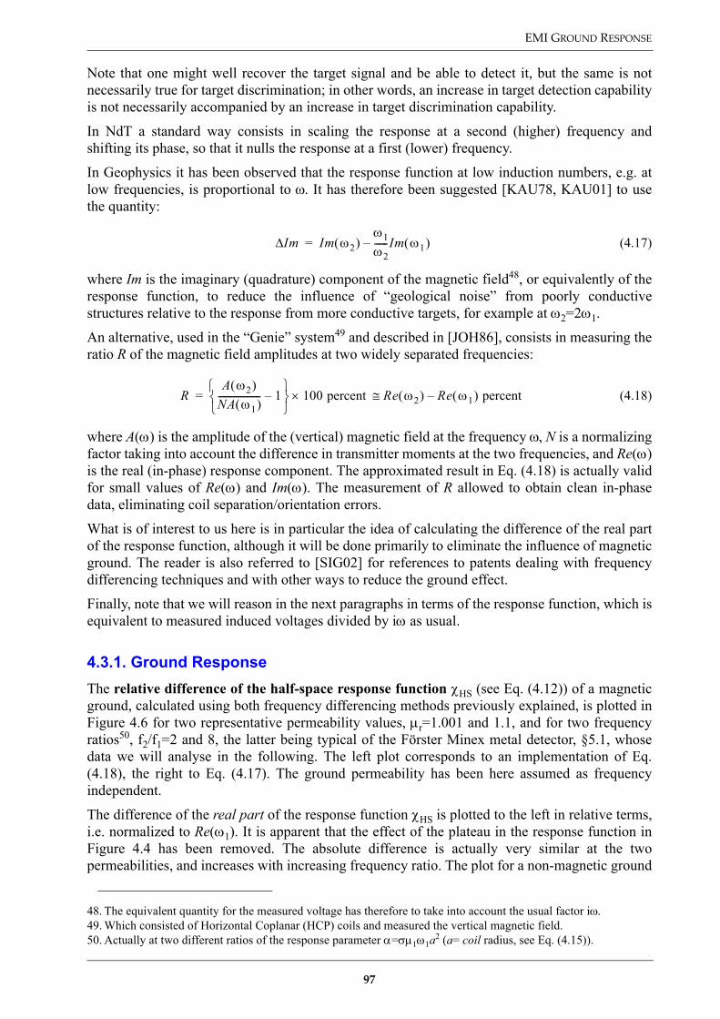
EMI GROUND RESPONSE
Note that one might well recover the target signal and be able to detect it, but the same is notnecessarily true for target discrimination; in other words, an increase in target detection capabilityis not necessarily accompanied by an increase in target discrimination capability.
In NdT a standard way consists in scaling the response at a second (higher) frequency andshifting its phase, so that it nulls the response at a first (lower) frequency.
In Geophysics it has been observed that the response function at low induction numbers, e.g. atlow frequencies, is proportional to ω. It has therefore been suggested [KAU78, KAU01] to usethe quantity:
(4.17)
where Im is the imaginary (quadrature) component of the magnetic field48, or equivalently of theresponse function, to reduce the influence of “geological noise” from poorly conductivestructures relative to the response from more conductive targets, for example at ω2=2ω1.
An alternative, used in the “Genie” system49 and described in [JOH86], consists in measuring theratio R of the magnetic field amplitudes at two widely separated frequencies:
(4.18)
where A(ω) is the amplitude of the (vertical) magnetic field at the frequency ω, N is a normalizingfactor taking into account the difference in transmitter moments at the two frequencies, and Re(ω)is the real (in-phase) response component. The approximated result in Eq. (4.18) is actually validfor small values of Re(ω) and Im(ω). The measurement of R allowed to obtain clean in-phasedata, eliminating coil separation/orientation errors.
What is of interest to us here is in particular the idea of calculating the difference of the real partof the response function, although it will be done primarily to eliminate the influence of magneticground. The reader is also referred to [SIG02] for references to patents dealing with frequencydifferencing techniques and with other ways to reduce the ground effect.
Finally, note that we will reason in the next paragraphs in terms of the response function, which isequivalent to measured induced voltages divided by iω as usual.
4.3.1. Ground ResponseThe relative difference of the half-space response function χHS (see Eq. (4.12)) of a magneticground, calculated using both frequency differencing methods previously explained, is plotted inFigure 4.6 for two representative permeability values, µr=1.001 and 1.1, and for two frequencyratios50, f2/f1=2 and 8, the latter being typical of the Förster Minex metal detector, §5.1, whosedata we will analyse in the following. The left plot corresponds to an implementation of Eq.(4.18), the right to Eq. (4.17). The ground permeability has been here assumed as frequencyindependent.
The difference of the real part of the response function χHS is plotted to the left in relative terms,i.e. normalized to Re(ω1). It is apparent that the effect of the plateau in the response function inFigure 4.4 has been removed. The absolute difference is actually very similar at the twopermeabilities, and increases with increasing frequency ratio. The plot for a non-magnetic ground
48. The equivalent quantity for the measured voltage has therefore to take into account the usual factor iω.49. Which consisted of Horizontal Coplanar (HCP) coils and measured the vertical magnetic field.50. Actually at two different ratios of the response parameter α=σµ1ω1a2 (a= coil radius, see Eq. (4.15)).
Im∆ Im ω2( )ω1ω2------Im ω1( )–=
RA ω2( )
NA ω1( )------------------- 1–
100 percent Re ω2( )≅× Re ω1( ) percent –=
97

CHAPTER 4
(µr=1) would not have shown a significant gain with respect to measuring the real part at thehighest of the two frequencies, as can be deduced from Figure 4.2. Finally, note that in the case ofa superparamagnetic ground this simple difference might have to be replaced with one including alogarithmic frequency factor (see Eq. (4.4)).
The difference of the imaginary part of the response function χHS is plotted to the right, again inrelative terms, i.e. normalized to Im(ω1). The curves for the different permeability values arepractically coincident. The differencing effectiveness gets again worse for increasing frequencyratios.
In practice the differencing scheme corresponding to the plot on the left is usually employed tosuppress the effect of magnetic soil (for example by the Förster Minex), the one corresponding tothe right plot to suppress the effect of conductive soils.
Frequency differencing methods will obviously affect the target response as well. We willtherefore look in the next paragraph at the overall response of a sphere, a representative targetwhose response function we already discussed in detail in Chapter 3.
4.3.2. Sphere ResponseThe difference of a sphere’s response function χSPH, ferromagnetic and non (µr=10 and µr=1respectively), calculated again using both frequency differencing methods previously explained,is plotted in Figure 4.7 for the same frequency ratios51 as above starting from Eq. (3.14). Thecontinuous curves correspond to the standard response at f1. The left plot corresponds again to animplementation of Eq. (4.18), the right to Eq. (4.17).
Notice in particular how the response is reduced:• for targets with low response parameter (e.g. low conductivity and/or small size) in the case of
∆Im, and ∆Re for a ferromagnetic object in particular.• for target with high response parameter (e.g. high conductivity and/or large size) as well in the case
of ∆Re.resulting in a bell-shaped response curve peaking at some intermediate value of the responseparameter. In addition the magnitude of the difference curves decreases with decreasingfrequency ratio. Some care has therefore to be applied when using these types of differences,depending on the type of target sought.
Figure 4.6: Frequency differencing techniques applied to a magnetic half-space’s (ground) response functions, for f2=8f1 (continuous) and f2=2f1 (dashed). Right: the curves for µr=1.001 and 1.1 are basically coincident.
51. Actually at two different ratios of the response parameter α=σµ1ω1a2 (a= sphere radius, see Eq. (3.15)).
10�210�310�410�5Α
10�1
10�2
10�3
10�4
10�5
10�6
100ReREL ��Re�ΧHS�f1��Re�ΧHS�f2������Re�ΧHS�f1����
Μr�1.001, f2�8f1 f2�2f1
Μr�1.1 f2�2f1
f2�8f1
1.�10�6 0.00001 0.0001 0.001 0.01Α
0.001
0.002
0.005
0.01
0.02
0.05
ImREL ���Im�ΧHS�f1���f1�f2�Im�ΧHS�f2������Im�ΧHS�f1����
Μr�1.001, 1.1 f2�8f1
f2�2f1
98

EMI GROUND RESPONSE
4.4. On the Ground’s Influence on the Primary and Scattered Fields
We have already discussed in some detail in the previous chapter the response of a conductorembedded in a conductive medium, in a number of scenarios of interest. What we want to pointout here is that even in the case where the total secondary fields cannot be separated in acontribution due to the host medium alone plus a contribution due to the conductor situated infree space (see the discussion in §3.7 and Eq. (3.55)), a simplified response might still available,valid in particular for “small targets”.
We might indeed consider the ground effect on the primary and secondary fields as being in firstapproximation equivalent to a phase shift, i.e. a rotation in the complex plane, proportional tofrequency, and an attenuation of the primary field on its way to the target, with a similar effect onthe secondary field on its way back to the receiver (§3.2.1). When the host medium is conductivebut still relatively ease penetrated by the EM fields, and the transmit and receive locations areclose to the target, such a low-pass filtering behaviour is just a phase shift, and has beenapproximated in [NAB91,pp.36-38] with the following response function:
(4.19)
where d is the target depth, σ and µ1 are the ground conductivity and permeability, l is ahorizontal scale parameter (of the order of the coil radius in our case), and δ=(2/σµ1ω)1/2 is theskin depth in the soil (see also Table 3.2).
The previous response function applies directly to both the target vortex (eddy) and galvanicresponse (§3.7), if any. The total secondary fields are then obtained by adding the contributionfrom the ground itself (host response). This effect is likely not to represent a problem in ourapplication, perhaps with the exception of high conductivity ground and/or for deep objects, andwhen operating at higher frequencies. In these cases it would however introduce a change intarget signature, which could not simply be compensated by subtracting the ground responsemeasured in the absence of the target.
Figure 4.7: Frequency differencing techniques applied to a sphere’s response function, non-magnetic (top) and magnetic (bottom, µr=10), for f2=8f1 (dashed) and f2=2f1 (dot-dashed). In red (continuous): –Re[χ],–Im[χ] at f1.
10�1 100 101 102 103 104Α0
0.2
0.4
0.6
0.8
1Re Re�ΧSPH�f1���Re�ΧSPH�f2�� �Μr�1�
10�1 100 101 102 103 104Α0
0.05
0.1
0.15
0.2
0.25
0.3
0.35
Im �f1�f2�Im�ΧSPH�f2���Im�ΧSPH�f1�� �Μr�1�
10�1 100 101 102 103 104Α�1.5
�1
�0.5
0
0.5
Re Re�ΧSPH�f1���Re�ΧSPH�f2�� �Μr�10�
10�1 100 101 102 103 104Α0
0.1
0.2
0.3
0.4
0.5
0.6
Im �f1�f2�Im�ΧSPH�f2���Im�ΧSPH�f1�� �Μr�10�
T 2iσµ1ωld–[ ]exp≅ 4il dδ2-----–exp=
99
CHAPTER 4
4.5. Conclusions
Soil effects, whose presence we have recognized early on during this work and which are oftennot sufficiently considered in the existing scientific literature related to humanitarian deminingapplications, have been calculated in this chapter by studying the response of a circular loop in ahomogenous half-space model, for different soil permeabilities and (normalized) detector heights.This has allowed to confirm in quantitative way their importance (for FD systems in particular).We have also drawn attention to superparamagnetic effects, which can play a role under certainconditions.
The role of the soil’s permeability, which heavily affects the real part of the response function,has been clearly shown (plateau effect at low frequencies). The imaginary part is on the otherhand linear in the response parameter (induction number). The latter is of the iωσµa2 form,confirming the dimensional analysis of A3.3.1. The effects of changes in the detector’s height arealso apparent, in particular on the real part of the response function for magnetic soils.
These dependencies can also be extrapolated to give an idea of the importance of fluctuations inthe ground’s parameters (inhomogeneities, height profile fluctuations), which will inevitably bepresent in real conditions, and which are also clearly documented in the experimental data ofChapter 5. For example, a 10% fluctuation in soil permeability will be roughly equivalent to asimilar fluctuation in the imaginary component of the induced voltage, and therefore be moreimportant in absolute terms when working in difficult ground conditions (high permeability).
Frequency differencing methods to reduce soil effects have also been described, and two ofthem studied in more detail. The half-space model has allowed us to understand why they workand to assess in a quantitative way how well they work; at the same time we have shown what isthe price to pay in terms of reduction of the target’s response in the case of a sphere. This will alsohelp in understanding the behaviour of the experimental data in Chapter 5 and in the analysis offeatures more robust to background fluctuations (Chapter 6).
Some of these results have obviously already been known to the metal detector community fromthe experimental point of view for a certain time, and partly to the geophysical community aswell, although the latter does usually put less emphasis on the ground’s permeability. Wetherefore see added value in having joined the two ends, putting together this information in acoherent way with emphasis on humanitarian demining specificities, and with the necessaryscientific rigour.
We have hereby finished setting the theoretical framework, and can now move to the analysis ofthe experimental data.
100
EMI GROUND RESPONSE
Bibliography
[BEA98] Beard, L., and Nyquist, J. E., 1998, Simultaneous inversion of airborne electromagnetic data forresistivity and magnetic permeability: Geophysics, v. 63, no. 5, September-October, p. 1556-1564.
[BLI97] Blitz, J., 1997, Electrical and Magnetic Methods of Non-destructive Testing: Chapman & Hall,London, UK.
[CHE65] Cheng, D. H. S., 1965, The Reflected Impedance of a Circular Coil in the Proximity of a Semi-Infinite Medium, IEEE Transactions on Instrumentation and Measurement, v. IM-14, no. 3, p.107-116.
[DOD68]Dodd, C. V., and Deeds, W. E., 1968, Analytical Solutions to Eddy-Current Probe-CoilProblems: Journal of Applied Physics, v. 39, no. 6, May, p. 2829-2838.
[DOD69]Dodd, C. V., Deeds, W. E., and Luquire, J. W., 1969, Integral Solutions to some Eddy CurrentProblems: International Journal of Nondestructive Testing, v. 1, p. 29-90.
[HUA01]Huang, H., and Fraser, D. C., 2001, Mapping of the resistivity, susceptibility, and permittivityof the earth using a helicopter-borne electromagnetic system: Geophysics, v. 66, no. 1, January-February, p. 148-157.
[IGN85] Ignetik, R., Thio, Y.-C., and Westfold, K. C., 1985, Transient electromagnetic field above apermeable and conducting half-space: Geophysical Journal of the Royal Astronomical Society,v. 81, p. 623-639.
[JOH86] Johnson, I. M., and Doborzynski, Z. B., 1986, A novel ground electromagnetic system:Geophysics, v. 51, no. 2, February, p. 396-409.
[KAU78]Kaufman, A. A., 1978, Resolving capabilities of the inductive methods of electro-prospecting:Geophysics, v. 43, p. 1392-1398.
[KAU89]Kaufman, A. A., 1989, A Paradox in Geoelectromagnetism, and its Resolution, Demonstratingthe Equivalence of Frequency and Transient Domain Methods: Geoexploration, v. 25, p. 287-317.
[KAU01]A. A. Kaufman, and P. A. Eaton, The Theory of Inductive Prospecting. Amsterdam, NL:Elsevier, 2001.
[KEL66] G. V. Keller, and F. C. Frischknecht, Electrical Methods in Geophysical Prospecting. Oxford,UK: Pergamon Press, 1966.
[LEE74] Lee, T., and Lewis, R., 1974, Transient EM response of a large loop on a layered ground:Geophysical Prospecting, v. 22, p. 430-444.
[LEE84] Lee, T., 1984, The transient electromagnetic response of a magnetic or superparamagneticground: Geophysics, v. 49, no. 7, July, p. 854-860.
[MOR69]Morrison, H. F., Phillips, R. J., and O’Brien, D. P., 1969, Quantitative interpretation of transientelectromagnetic fields over a layered half-space: Geophysical Prospecting, v. 21, p. 1-20.
[NAB87]Nabighian, M. N. (Ed.), 1987, Electromagnetic Methods in Applied Geophysics, Volume 1,Theory: Investigations in Geophysics No. 3, Society of Exploration Geophysicists (SEG),Tulsa, OK, USA.
[NAB91]Nabighian, M. N. (Ed.), 1991, Electromagnetic Methods in Applied Geophysics, Volume 2,Application: Investigations in Geophysics No. 3, Society of Exploration Geophysicists (SEG),Tulsa, OK, USA.
[OAT92] Oaten, S. R., and Blitz, J., 1992, Impedance analysis for air-cored cylindrical eddy current coilsscanning the surfaces of defect-free conductors: Nondestructive Testing and Evaluation, v. 6, p.323-335.
[RYU70]Ryu, J., Morrison, H. F., and Ward, S. H., 1970, Electromagnetic fields about a loop source ofcurrent: Geophysics, v. 35, no. 5, October, p. 862-896.
[SIG02] Sigrist, C., and Bruschini, C., “Metal Detectors for Humanitarian Demining: a Patent Search
101

CHAPTER 4
and Analysis”, EUDEM2 report, May 2002. Available from http://www.eudem.vub.ac.be/[SPI91] Spies, B. R., and Frischknecht, F. C., 1991, Electromagnetic Sounding, in [NAB91], p. 285-
425.[THO77] Thomas, L., 1977, Electromagnetic Sounding with Susceptibility among the Model Parameters:
Geophysics, v. 42, no. 1, February, p. 92-96.[WAI79] Wait, J. R., 1979, Review of Electromagnetic Methods in Nondestructive Testing of Wire
Ropes: Proc. of the IEEE, v. 67, no. 6, June, p. 892-903.[WAI82] Wait, J. R., 1982, Geo-electromagnetism: Academic Press, New York.[WAR87]Ward, S. H., and Hohmann, G.W., 1987, Electromagnetic Theory for Geophysical
Applications, in [NAB87], p. 130-311.
102

5. Metal Detector Raw Data Analysis
In order to i) compare the experimental data with theoretical expectations, ii) getqualitative indications of a CW (Continuous Wave) metal detector response toobjects of interest in humanitarian demining (mines and clutter), and iii) analyse thepossibility of identifying targets of interest, or at least discriminating some metallicobjects based on their characteristic response (in particular the phase), we haveacquired and analysed an extensive amount of metal detector raw data using acommercially available differential CW system, the Förster Minex 2FD.
We have recorded the detector’s internal signals, i.e. the in-phase and quadrature-phase component at each frequency, as well as the difference of the two quadrature-phase components and the audio signal available to the operator. Experimental datahas been acquired by varying different object parameters, in a laboratory setup withthe objects either flush or buried. Linear scans, and in some cases series of parallelscans as well, have been carried out with a high density of points in the scandirection, placing the detector on a Cartesian gantry.
Scans of general interest will be detailed first (§5.2), followed by an analysis of theresponse of reference objects (spheres, cylinders, etc.; §5.3), of the response variationwith distance (§5.4), with axial offsets (2D parallel scans; §5.5) and with the object’sorientation in the horizontal plane (§5.6). Detailed responses will then be shown for aminimum-metal mine and its components (§5.7), a PMN mine (medium metal contentmine; §5.8), metallic mines (PROM, PMR-2A) and a composite UXO example (§5.9).Finally, several tens metallic clutter pieces will be looked at (§5.11). Overall results willbe extensively summarized at the end of the chapter (§5.12). No particular attempt atbackground subtraction has been done other than the subtraction of the mean values(to remove offsets).
The collection of data as a function of movement enables the possibility of analysingthe data in the complex, or impedance, plane (in-phase vs. quadrature-phasecomponent). This method resembles measurements carried out in Non-DestructiveTesting (NdT), from where it was inspired, and makes it possible to exploit globalobject properties rather than only local ones.
103

CHAPTER 5
5.1. The Förster Minex Metal Detector
This Förster Minex 2FD is a CW system which generates two continuous wave frequencies, at2.4 kHz and 19.2 kHz. The first frequency is aimed in particular at the detection of ferromagneticobjects, the second at the detection of stainless steel and alloys, in agreement with the modellingresults of Chapter 3 and the corresponding frequency dependence.
The transmitter of the Förster Minex 2FD consists of a conventional copper coil (diameter 230mm), whereas its receiver is composed of an eight-layer printed circuit board (diameter 200 mm),coaxial and coplanar with the transmitter, arranged as a gradiometer (see Figure 5.1).
This results in a differential left-right system, its output audio signal vanishing (no tone) when thedetector’s mid axis crosses the object’s centre, thus allowing a very precise spatial localisationalong one dimension as schematically represented in Figure 5.2, with the standard responseshown for comparison. The differential setup also helps in background suppression and enhancesthe separation power (localizing nearby objects). On the other hand mechanical tolerances arestricter, and sensitivity is probably somewhat reduced, given that the receiving coil has been splitinto two, effectively halving the sensitive area.
The physical quantity which the detector measures is therefore an approximation of the gradientof the induced magnetic field (actually its vertical component) along a direction perpendicular tothe detector’s axis, i.e. when working as shown in Figure 5.2.
Figure 5.1: Förster Minex 2FD detector head on gantry support frame [BRU00b].
Figure 5.2: Differential response, and standard response for comparison (both qualitatively), for a linear scan along x
SCANNING SETUP (top view)
DIFFERENTIAL RESPONSE
V (amplitude)
xx
differentialmetal detector
scanning line
object center
V (amplitude)
object center
“STANDARD” RESPONSE
x1 2 3
1
2
3
x=0
y
Bzsec∂ x∂⁄
104

MD RAW DATA ANALYSIS
To fully exploit the detector’s capabilities we intercept, at the output of the receiver-transmittermodule, five signals (f10°, f190 °, f20°, f290°, Delta) corresponding respectively to the real (f10°,f20°, or equivalently f1 REAL and f2 REAL) and imaginary parts (f190°, f290°, or equivalently f1IMAG and f2 IMAG) (in the complex plane) of the analog signals and induced at f1 andf2 in the receiver, and the difference of the imaginary parts multiplied by a constant(Delta=c(f190°–f290°)), which turns out to be quite insensitive to changes in (back)groundconditions.
These internal signals are normally not available to the standard user and do not depend on thesensitivity setting. They are continuously analysed by a microprocessor which delivers an output(Audio), the standard audio signal (i.e. what the operator would hear), relying mostly on the Deltasignal. The Audio signal depends heavily on the sensitivity chosen52.
The induced voltages and are amplified by a factor F1 and F2 respectively, which arechosen to satisfy the following relationship (I1 and I2 are the currents in the primary coil at f1 andf2 respectively):
(5.1)
This scaling effectively removes the linear dependency on ω of the induced voltage (see forexample Eq. (3.13)) and makes it possible to use the Delta signal defined before to suppress thesoil influence. It also allows us to compare the ratios and trends of the induced voltages withthose of the response function χ.
The real part is again often referred to as “in-phase”, the imaginary part as “quadrature-phase”component, whereby the phase is measured with respect to the transmitted signal shifted by aconstant amount (a few degrees), representing a reference angle which corresponds to a typicalmagnetic soil. This phase shift stays constant unless a “ground cancellation (balancing)procedure”, one of the detector’s options, is explicitly performed. A slow “ground following”adaptation function is also implemented.
Note that a magnetic object, e.g. ferrite, would deliver a purely quadrature phase signal (90°phase shift).
Typical signals are shown in Figure 5.3 and Figure 5.5 taking as example the object representedin Figure 5.4, bottom left (striker pin of a minimum-metal mine). Data collection has been carriedout in a straight line across the object’s centre, recording the signals with a dedicated 16 bitconversion card over +/–5 Volt every 0.56 mm (about 2 points per mm); the data acquisition cardand gantry which make this possible have been realised by Frédéric Guerne at the EPFL.
Typical scan lengths were between 60 and 100 cm with the detector at 2-3 cm above the groundunless otherwise specified. The data was then lowpass filtered with a simple sliding window 30 to90 data points wide53, and centred (subtraction of mean value to remove offsets). The Audiosignal was median filtered over 5 data points to eliminate outliers.
The detector’s differential response is clearly visible in Figure 5.3, where “Left” has beenassigned to lower value coordinates. When moving in the direction of increasing coordinates –from “Left” to “Right” – a first peak is traversed to the left of the object (“LeftPeak”); the objectcentre then comes at about x=600 mm, followed by a second peak to the right of the object(“RightPeak”). Note that the signal for such a small and shallow object is about as wide as thedetector head itself.
52. Three different levels of sensitivity (1, 2 and 3) are user-selectable. Default is 1 (lowest), 3 is equivalent toextremely sensitive.
53. Actually the MATLAB® “filtfilt” function was used (zero-phase forward and reverse digital filtering); theeffective filter order is therefore twice the figure quoted.
V1s( ) V2
s( )
V1s( ) V2
s( )
F1 ω1 I1⋅ ⋅ F2 ω2 I2⋅ ⋅=
105

CHAPTER 5
The imaginary components show large fluctuations outside the zone of interest, probably due tosoil inhomogeneities and/or surface height variations; these fluctuations are in fact stronglycorrelated and the imaginary signals practically overlapping. The resulting difference (Delta) istherefore non zero only in correspondence of the target. The real components are on the otherhand clean and unambiguous in the given experimental conditions. Note that the Audio signalresults from a thresholding, towards positive and negative values, of the sole Delta signal; theformer is measured by our data acquisition system as unipolar, but is in fact bipolar – a differenttone is emitted for each polarity, which greatly eases pinpointing. The object’s centre is in aposition corresponding to the dip in between the peaks of the audio signal at x=600 mm, incorrespondence of the zero crossing of Delta.
Standard Scanning SetupAfter having checked that the soil is free of metallic objects, scans were carried out using thestandard parameters detailed in A5.1 (unless otherwise indicated).
Summarising, linear scans, and in some cases series of parallel scans as well, have been carriedout with a high density of points in the scan direction, placing the detector on a Cartesian gantry[BRU98a]. The latter has been transferred in 1998 from the EPFL in Lausanne, where initial datacollections have taken place [BRU98a, BRU98b], to the VUB in Brussels. Preliminary resultshave been detailed in [BRU00b].
A number of mines to which we will often refer in the following are grouped in Figure 5.4, whichdetails in particular their metallic content.
Figure 5.3: Typical processed (i.e. filtered and entered) internal and Audio signals from the Förster Minex 2FD metal detector [BRU00b].
200 300 400 500 600 700 800 900 1000 1100−10
−5
0
5
10
V (
mV
olt)
Processed Amplitudes vs. Distance along Scan
f1 REALf2 REAL
200 300 400 500 600 700 800 900 1000 1100
−20
−10
0
10
20
V (
mV
olt)
f1 IMAGf2 IMAGDELTA
200 300 400 500 600 700 800 900 1000 11000
100
200
300
400
X (mm)
V (
mV
olt)
AUDIO
Left
LeftPeak
Right
RightPeak
ObjectCentre
106

MD RAW DATA ANALYSIS
Amplitude RatioApart from the phase response behaviour there is an additional parameter of interest on which wewill comment in this chapter in a qualitative way, the ratio of the amplitudes of the received signalat the two frequencies (Amplitude Ratio, or AR). It will be defined in §6.2.2 and its distributionanalysed in more detail in §6.2.6.
Figure 5.4: Metallic content of a Russian PMN (pmnCambodia; top left), a Russian PMN2 (top right), and an LI11 min.-metal mine (mich; bottom left), with detail of striker pin (mist) and original detonator (midereal, bottom
right). (Source: EPFL/DeTeC)
107

CHAPTER 5
5.2. Data Collection Results: Scans of General Interest
We will detail in this paragraph the detector’s response for scans of general interest, i.e. mostlyaimed at sensor and environment understanding and characterization. No particular attempt atbackground subtraction has been done other than the subtraction of the mean values alreadydescribed (to remove offsets).
For each data point in the complex plane we can obviously calculate a magnitude and a phasealong the lines discussed in §2.2.4. When the phase response of the received signal changes littleover the whole scan we get diagonal lines and the phase is nothing else but their slope. When thisis not the case, either because the object has a characteristic phase response or because thebackground signal is prevailing, or both, there might still exist a general trend which can be usedto calculate an “average phase”. Another possible choice is for example to take the phase wherethe signal is strongest [SZY99], at the positions we previously labelled “LeftPeak” and“RightPeak”. We will concentrate here on the qualitative aspects of the received signal (thecurves’ slopes and shapes). A quantitative analysis of the phase response will be undertaken inChapter 6.
Raw vs. processed data in the complex plane and background fluctuation effectsThe right half of Figure 5.5 shows the processed data from Figure 5.3, plotted this time directly inthe complex (impedance) plane and taken around the area of interest only (from x=450 mm tox=750 mm). The left half of Figure 5.5 shows the raw data from the same acquisition, that is alldata unprocessed; the sets of data points at the two frequencies are well separated, due to thesignals having different offsets. These offsets seem to be rather constant.
In this particular case the background fluctuations, probably due to soil inhomogeneities asdiscussed before, are not negligible and the corresponding curves in the complex plane aredistorted, in particular at f2. The target signals, corresponding to the diagonally lying sets ofpoints, are however still strong enough and we can rather clearly separate them in the left half of
Figure 5.5: Raw and processed internal signals (see also Figure 5.3) plotted in the complex plane [BRU00b]
−80 −70 −60 −50
−50
−40
−30
−20
−10
0
10
20
f1 REAL (mVolt), f2 REAL (mVolt)
f1 IM
AG
(m
Vol
t), f
2 IM
AG
(m
Vol
t)
RAW data
−5 0 5
−2
0
2
4
6
8
10
12
14
16
18
f1 REAL (mVolt), f2 REAL (mVolt)
f1 IM
AG
(m
Vol
t), f
2 IM
AG
(m
Vol
t)PROCESSED data, around area of interest
f1f2
f1
f2
Left
Right
Left
Right
LP: LeftPeak
ObjectCentre
ObjectCentre
RP: RightPeak
LP1
LP2
RP1
RP2
108

MD RAW DATA ANALYSIS
the image from the background signals54 (the fluctuating imaginary component which translatesinto vertically distributed data points). This is unfortunately not always the case.
Soil 2D ScansDetailed soil scans (sand) were carried out at the EPFL and the VUB sandbox. Under theseconditions reproducible fluctuations are clearly visible in the imaginary components (f190°,f290°), at the mV level (Figure 5.6) and basically identical for both components. They are mostlikely due to fluctuations in soil homogeneity and/or ground profile. Fluctuations in the realcomponent (f10°,f20°) are at the noise floor level (of the order of 0.1 mV) and are not shown. Thisbehaviour is consistent with the modelling results of Chapter 4 for a resistive paramagneticground.
These 2D scans were taken, as most of the following ones, over a surface of 500×800 mm with 26parallel scans, separated by 2 cm, along the y axis (y is the along track coordinate).
Additional scans were taken after having disturbed the sand surface, in particular (bgnd3v2)after having disturbed the surface in the upper right (455,655) and lower left corner (140,192),and (bgnd3v3) after having dug a conical hole (30 cm dia, 15 cm depth at lowest point) in thecentre (210, 446), removing the sand from the test area. bgnd1v2 represents undisturbed soil,see Figure 5.7.
Differences are clearly visible, although it is not straightforward to relate them to the action taken(e.g. the hole should be in the centre!). This could point to additional (electronics?) filteringeffects, which are not apparent under normal operating conditions aimed at the detection of smallhigh conductivity targets.
54. Which have been cut in the right half of the image as already said.
Figure 5.6: 2D soil scan (sand), f190°. z: Amplitude (in mV).
YX
0
200
400
600
800
0
100
200
300
400
500−4
−3
−2
−1
0
1
2
3
mm (along track coordinate)
2D soil scan: measVUB1/bgnd1, f190, 06042001, h025
mm
mV
109

CHAPTER 5
Other Soil ScansA one dimensional scan of a Cambodian soil sample (lateritic earth) is shown in Figure 5.8. Asmall quantity of sand has been taken out of the sandbox, in the centre of a 1D scan, and replacedby the test earth sample; a localized anomaly is therefore generated. A small but clear “magnetic”response is visible (imaginary components), equal at both frequencies, corresponding to a phaseangle of about 2-3°. Another Cambodian sample was analysed in the same way; no appreciabledifference with the surrounding sand was remarked.
Forward/Reverse ScansScans were carried out along the same line and over the same object once in “forward” (i.e. withincreasing along track coordinate value) and once in “reverse” direction. No signal differenceswere recorded, apart from a shift of 5-7 pixels (2.5-3.5 mm) possibly due to the gantry itself or tothe (electronics) filtering effects previously described.
Figure 5.7: 2D soil scan (sand), f190°, after having disturbed the surface twice (see text).
0200
400600
800
0100
200300
400500
−2
−1
0
1
2
mm (along track coordinate)
measVUB4: bgnd1v2−bgnd3v2 (disturbed soil surface), f190, 30102001, h025
mm
mV
0200
400600
800
0100
200300
400500
−3
−2
−1
0
1
2
mm (along track coordinate)
measVUB4: bgnd2v2−bgnd2v3 (hole in centre), f190, 30102001, h025
mm
mV
110

MD RAW DATA ANALYSIS
All 3 Sensitivity LevelsIdentical scans were carried out varying the sensitivity level. The Audio signal does obviouslychange, all others are practically the same apart from a possible shift of +/–1 pixel, likely due tothe gantry. Figure 5.9 presents an example of the Audio output for a small steel sphere (sts1)and a large one (sts4).This test does also constitute a measure of drift effects, which were notnoticed on this time scale (several minutes).
Second MD HeadAll acquisition carried out at the EPFL sandbox used one and the same MD head, shown inFigure 5.1. As this was slightly damaged it was decided to employ a second head for most of thedata acquisition carried out at the VUB, keeping the same electronics. No differences in responsewere noticed.
Figure 5.8: 1D scan over a lateritic soil sample (origin: Cambodia).
Figure 5.9: Audio output (3 sensitivity levels) over sts1 (Left) and sts4 (Right) (s=1: green, s=2: red, s=3: blue). x: samples, y: signal amplitudes (mV)
−3 −2 −1 0 1 2 3
−2.5
−2
−1.5
−1
−0.5
0
0.5
1
1.5
2
2.5
f10, f20, mV
f190
, f29
0, m
V
MeasVUB7/earth2 (Cambodia soil sample) f1 f2 filtfilt order 75
f1f2
0 500 1000 15000
100
200
300
400
500
600
700sts1, Audio, 3 sensitivities
0 500 1000 1500−200
0
200
400
600
800
1000
1200sts4, Audio, 3 sensitivities
111

CHAPTER 5
Background (Soil) Signal SubtractionMost of the scans have been carried out on objects placed on the surface (usually for smallobjects) or just underneath it (flush), to ease data acquisition while at the same time taking intoaccount the response from the soil itself, at least to first order. The latter is not negligible, evenunder these conditions, when looking at some of the smaller objects. Background (soil) scans, i.e.without target, should therefore ideally be taken for each object in 1D (along a line) or 2D(parallel lines).
As a compromise we decided to take background scans before and after each series of scans, forexample when measuring different spheres one after the other under the same conditions. Thesebackground scans were then compared. In some cases there was a weak offset, which does notrepresent a serious drawback; a difference between the f190° and f290° channels was recorded insome cases as well in the centre of the scan (where the target objects were buried). Although thiswas generally not a problem, it implies that the background (soil) can change as a consequence ofthe measurement procedure (putting the object/s in place and removing it/them), and thatindividual background scans have to be performed when the highest measurement precision isrequired and/or the signals are very weak.
Normalized PlotsMetal detector data is quite often characterized by large amplitude differences from one scenarioto the other. In order to be able to compare them we will often normalize the complex plane databy dividing each data point – its real and its imaginary part – by the maximum of the amplitude inthe complex plane (each frequency separately). As the phase angle of each point does not changethis transformation preserves the plot’s aspect ratio. A normalized plot’s scales are adimensional.
Typical Scan ConfigurationsFigure 5.10 reproduces the most typical data acquisition scenarios. The corresponding data willbe described in the following paragraphs.
See also A5.2 for a Glossary of the terms used in the following and A5.3, A5.4 for a list ofFilename and Object codes.
Figure 5.10: Typical data acquisition scenarios
h3
h2
h1
hPER
PAR
d
1D Scans at different HEIGHTS 2D PARALLEL scans 1D scans at fixed height, differentORIENTATIONS (HORIZ. plane)
MD
Target
Target
Target
112

MD RAW DATA ANALYSIS
5.3. Reference Objects
Before moving to more complex objects and scenarios it is useful to study the response ofcanonical targets such as spheres, cylinders, loops and magnets.
Spheres (sts1-sts4)The non-normalized responses of the four reference steel spheres (sts1 to sts4) are plotted inFigure 5.11 (offsets have not been subtracted): the phase angles are decreasing (the straight linesrotate in clockwise direction) when moving from f1 to f2 and from a smaller sphere to a largerone, in agreement with the modelling results of §3.4.5.2.
The amplitude ratio AR (see §6.2.2) is well above 1 for sts1, the smallest sphere, and decreaseswhen moving towards sts4, in agreement with §6.2.6.
Cylinders1D non-normalized responses for all cylinders except msc2 (large: cyl2, small: cyl1), placedperpendicularly to the scanning direction (PER orientation), are shown in Figure 5.12, whichconfirms the expected phase and amplitude trends for increasing conductivity and is similar to theone for a sphere.
The amplitude ratio is >1 for aac1,2 (ferromagnetic), <<1 for alc1,coc1, and <1 foralc2,coc2 (aluminium and copper). This is again in agreement with §6.2.6, even if thecylinders are of finite length.
AR is quite small for the inc1,2 stainless steel cylinders (about 1/3 and 1/7 respectively), andtheir response is quite weak as well, especially at f1. Also, their phase is positive for inc1 at bothfrequencies (practically invisible in the f1 plot), and at f1 for inc2 as well (barely visible). This isin principle non possible for a non-ferromagnetic object, and might be explained with a smallresidual permeability of the stainless steel55.
Figure 5.11: Steel spheres. Top: sts3 (red, smallest amplitudes), sts4 (blue). Bottom: sts1 (blue, smallest amplitudes), sts2 (red). Scales are in mV. x: f10,f20; y: f190,f290.
55. One could therefore discriminate between the stainless steel situation (phases>0) and that of a ferromagneticobject (§5.9) by looking at the amplitude ratio.
−2000 −1500 −1000 −500 0 500 1000 1500 2000
−500
0
500
sts3 (red) vs sts4 (blue), first and second freq,
−200 −150 −100 −50 0 50
−40
−20
0
20
40
sts1 (blue) vs sts2 (red), first and second freq,
113

CHAPTER 5
Comparison between Vertically/Horizontally placed objects (VER vs. PAR, PER configs.):• Ferromagnetic (Figure 5.13): the shape of the VER curve is a straight line (like for PER), the
phase is however closer to the one of PAR (especially the straight section), possibly because thecontribution from the field along the cylinder axis is dominant. These effects are consistent withwhat seen in §3.5.2 (orientation sensitivity of short ferromagnetic parts).
• Non-ferromagnetic: tests were carried out with the copper reference cylinders (coc2 and coc1).In general nearly identical phases are recorded for all orientations56, with small differencesbetween the vertical setup and the other configurations. PAR, PER, QU1 and QU4 havecomparable amplitudes, larger than VER (which is not astonishing, given that in the vertical setupthe top of the object is flush; its bulk is therefore buried and farther from the sensor). Similarresults should hold for other non-ferromagnetic objects.
• Other studies dealing with orientation effects (not only for cylinders): Results for differentorientations in the vertical plane are reported in [KEI98, COL99b] for GEM-3 UXO data;[CHE84] also reports significant differences for prolate steel spheroids, using TD equipment.Horizontal vs. vertical orientation differences are reported in [TRA97] for several mines usinglaboratory FD equipment. Most data is acquired for the target in a fixed spatial position, [KEI99]representing an exception.
Figure 5.12: Response at f1 (Left) and f2 (Right) for all ref. cylinders (except msc2), placed perpendicularly to the scanning direction (PER orientation). Left: “small” cylinders, Right: “large” cylinders. Not normalized.
Figure 5.13: Response at f1 and f2 to a mild steel cylinder (msc2) for different orientations. Left: VER vs. PAR, Right: VER vs. PER. Normalized.
56. Horizontal orientations are described in A5.2.
−10 −5 0 5 10
−20
−15
−10
−5
0
5
10
15
20
cyl1 PER Test 7.3.1 h=025 f1
f10, mV
f190
, mV
alc1coc1inc1aac1
−50 0 50
−100
−50
0
50
100
cyl2 PER Test 7.3.1 h=025 f1
f10, mV
f190
, mV
alc2coc2inc2aac2
−10 −5 0 5
−15
−10
−5
0
5
10
15
cyl1 PER Test 7.3.1 h=025 f2
f20, mV
f290
, mV
alc1coc1inc1aac1
−50 0 50
−80
−60
−40
−20
0
20
40
60
80
100
cyl2 PER Test 7.3.1 h=025 f2
f20, mV
f290
, mV
alc2coc2inc2aac2
−2.5 −2 −1.5 −1 −0.5 0 0.5 1 1.5 2 2.5
−0.5
0
0.5
f10
f190
MeasVUB5/msc2−000−025−1−2D−ver−test7.2.012 vs MeasVUB5/msc2−000−025−1−per−test7.2.001 (mean subtracted and norma
f1 first filef1 second file
−2.5 −2 −1.5 −1 −0.5 0 0.5 1 1.5 2 2.5
−0.5
0
0.5
f20
f290
f2 first filef2 second file
−2.5 −2 −1.5 −1 −0.5 0 0.5 1 1.5 2 2.5
−0.5
0
0.5
f10
f190
MeasVUB5/msc2−000−025−1−2D−ver−test7.2.012 vs MeasVUB5/msc2−000−025−1−par−test7.2.001 (mean subtracted and normal
f1 first filef1 second file
−2 −1.5 −1 −0.5 0 0.5 1 1.5 2
−0.6
−0.4
−0.2
0
0.2
0.4
0.6
f20
f290
f2 first filef2 second file
VER vs. PAR VER vs. PER
VER
PER
VER
PAR
114

MD RAW DATA ANALYSIS
Small Loop and MagnetA small loop and a permanent magnet are quite useful to understand the general response trends:very good conductor on one hand, ferromagnetic (high µr) non-conductive object on the other.
The very strong response57 from a closed loop (loo2, copper wire) is shown in Figure 5.14,bottom left (scales are in mV and mV×104), and clearly approaches the inductive limit (–90°) atf2, in agreement with §3.1. The response from a similar open loop (loo1, top left) is as expectedvery much lower, with the phase at f1 close to 0°.
The magnet’s response (mag1) in the complex plane is nearly vertical, with φ1~89°, φ2~90°(Figure 5.14, right). The response at f1 does indeed feature a small real component withamplitude~1 mV, whose origin is not immediately apparent (possible due to µr changing withfrequency?).
Non-ferromagnetic vs. Ferromagnetic ObjectFigure 5.15 represents well the difference between non-ferromagnetic objects and (small)ferromagnetic ones.
As an example of the first we have taken as an irregularly shaped, long and slender piece ofcopper, whose response is shown in the upper half; the real and imaginary components haveopposite polarity, which translates into a negative slope in the complex plane (the phase angle ofinterest here is the one measured in the fourth quadrant (+,–)). Aluminium and stainless steelwould, amongst others, behave in the same way.
As an example of the second we have taken a small mild steel cylinder (msc2), of diameter 7 mmand height 30 mm, placed flatly in the horizontal (xy) plane and transversally (PER orientation) tothe scanning direction. Its response is shown in the lower half of the image; the real andimaginary components have the same polarity, which translates into a positive slope in thecomplex plane (the phase angle of interest here is the one measured in the first quadrant (+,+)).
Note how the phase angle decreases from f1 to f2 in both cases. Notice also that the absolute valueof the response at f1 is larger than at f2 for the ferromagnetic object, the inverse for the copperpiece. These trends are consistent with the previous theoretical analysis of the response function’sbehaviour (Chapter 3). Again, the signals themselves are unfortunately not always as strong andregular as in this case, in which it is easy to differentiate the objects.
57. The signal at f2 is actually partially clipped.
Figure 5.14: Left: Small open loop (top), closed (bottom). Right: Small permanent magnet. Scales are in mV.
−10 −8 −6 −4 −2 0 2 4 6 8
−3
−2
−1
0
1
2
3
loop1, f1 (blue), f2 (red)
−1 −0.8 −0.6 −0.4 −0.2 0 0.2 0.4 0.6 0.8 1
x 104
−3000
−2000
−1000
0
1000
2000
3000
4000
loop2, f1 (blue), f2 (red)
−200 −150 −100 −50 0 50
−100
−50
0
50
100
mag1, h030, test6.6, z1 (r), z2 (b)
115

CHAPTER 5
Two Different Objects of the same TypeTests were carried out on pairs of visually identical reference steel spheres (sts1 to sts4). Thephase of the response was identical to about +/–1.5°, with the response for sts1 too weak tomake precise quantitative statement (there was however qualitative agreement).
Two Identical Spheres Placed in ContactThe average phase value of two identical spheres in contact are the same as those of a singlesphere of the same type, but the individual curves are slightly “figure 8” shaped (like in the caseof a parallel steel cylinder) as shown in Figure 5.16, left. The exact profile does probably dependon the position of the spheres with respect to the scanning direction.
Figure 5.15: Typical response of non-ferromagnetic vs. ferromagnetic objects [BRU00b]
Figure 5.16: Left: Two identical spheres placed in contact, compared with a single sphere of the same type (sts4). Right: Two different spheres placed in contact (sts3+sts4), compared with sts4.
600 800 1000 1200
−300
−200
−100
0
100
200
300
400
V (
mV
olt)
f1 REAL,IMAG f2 REAL,IMAG
f1f2
−400 −200 0 200 400−300
−200
−100
0
100
200
300
f1 IM
AG
(m
Vol
t), f
2 IM
AG
(m
Vol
t)
complex plane representation
f1f2
400 600 800 1000
−200
−100
0
100
200
X (mm)
V (
mV
olt)
f1f2
−200 −100 0 100 200
−200
−100
0
100
200
f1 REAL (mVolt), f2 REAL (mVolt)
f1 IM
AG
(m
Vol
t), f
2 IM
AG
(m
Vol
t)
f1f2
Non−ferromagneticobject (ex. copper scrap)
Ferromagneticobject (ex. mild steelcylinder)
−2.5 −2 −1.5 −1 −0.5 0 0.5 1 1.5 2 2.5
−0.5
0
0.5
f10
f190
MeasVUB4/sts4x2−000−025−1−test7.1.001 vs MeasVUB4/sts4−000−025−1−test6.5.001 (mean subtracted and normalized)
f1 first filef1 second file
−1.5 −1 −0.5 0 0.5 1 1.5−0.6
−0.4
−0.2
0
0.2
0.4
f20
f290
f2 first filef2 second file
−2.5 −2 −1.5 −1 −0.5 0 0.5 1 1.5 2 2.5
−0.5
0
0.5
f10
f190
MeasVUB4/sts3sts4−000−025−1−test7.1.001 vs MeasVUB4/sts4−000−025−1−test6.5.001 (mean subtracted and normalized)
f1 first filef1 second file
−1.5 −1 −0.5 0 0.5 1 1.5
−0.6
−0.4
−0.2
0
0.2
0.4
0.6
f20
f290
f2 first filef2 second file
116

MD RAW DATA ANALYSIS
Two Different Spheres Placed in ContactThe resulting phase values for this configuration are intermediate between those of the largest andthe smallest object, like those resulting from a simple vector sum, which is rigorously true onlyfor uncoupled objects (see §3.3.4). In the tested configuration they are however closer to thelargest object (the largest amplitude dominates); an example is provided in Figure 5.16, right, forsts3+sts4. This also implies that the combined object can look “smaller”, from the point ofview of the phase angle, than the largest of the two objects, although the overall object mass anddimension have obviously increased, as well as the total signal amplitude.
117

CHAPTER 5
5.4. Phase vs. Distance (depth)
Scans at increasing distance from the object were carried out raising the detector head in 1 or 2cm increments, without displacing the object; this is definitely easier than changing burial depth,even if obviously less realistic, and has the advantage that the influence of the background isreduced too as the height increases, not only the target signal.
Spheres (sts2, sts4)Up to about 10 cm in the case of sts2 and 16-18 cm for sts4 (both steel spheres) the phasesare basically identical, then the signals get too weak for a simple quantitative comparison58. Theresponses from the individual channels do obviously change, becoming broader at increasingdistance. No multipole effects are apparent for the large sphere, which is consistent with theanalysis of §3.4.4 for a sphere of this size.
Ferromagnetic Cylinders in the Horizontal PlaneThe response of a ferromagnetic cylinder (msc2) for each of the four orientations in theHORizontal plane (PAR, PER, QU1, QU4) is shown in Figure 5.17 at increasing detectorheights. The PER profiles do not change, whereas the PAR ones do and become somewhat moreirregular (larger variation in phase angles) with increasing height. An exception is the straightsection in each plot, which stays unchanged; it corresponds to the approach phase – up to the firstpeak say – and when moving away from the object, after the last peak say.
Similar comments apply for a small ferromagnetic cylinder (msc1, see Figure 5.18). In addition:the amplitude ratio (PAR vs. PER) changes with the height, and is closer to 1 at f2 than at f1. Theshapes are again quite complex in the PAR configurations, becoming more irregular withincreasing height; this effect is more marked than for msc2. The difference between the PAR andPER configurations is important, and is also more marked than for msc2.
Target in Vertical PlaneTests were carried out with a vertical reference copper cylinder (coc2). All scans at increasingheights featured nearly identical phases, and should hold for other non-ferromagnetic objects.Similar results have also been obtained for parallel scans at a fixed height (§5.5).
Scans at different heights were also analysed with a vertical msc2 cylinder, i.e. an elongatedferromagnetic object. The phase stays constant from one to the other. This is not true any more forparallel scans at a fixed height (see again §5.5).
Similar effects for prolate steel spheroids at a fixed orientation have been reported using a timedomain system in [CHE84].
58. Note that the detection limits are higher than the values just indicated.
118

MD RAW DATA ANALYSIS
Figure 5.17: Response at f1 (Top) and f2 (Bottom) to a mild steel cylinder (msc2) placed flush with the surface, at increasing detector heights for each of the four orientations in the horizontal plane. Normalized.
Figure 5.18: Response at f1 (Left) and f2 (Right) to a small mild steel cylinder (msc1) placed flush with the surface, at increasing detector heights for the PAR and PER orientations in the horizontal plane. Normalized.
−1 −0.5 0 0.5 1
−0.8
−0.6
−0.4
−0.2
0
0.2
0.4
0.6
msc2 Test 7.2.1 PAR f1 norm
f10, mV
f190
, mV
−1 −0.5 0 0.5 1
−0.5
0
0.5
msc2 Test 7.2.1 PER f1 norm
f10, mV
f190
, mV
h=025h=050h=100
−1 −0.5 0 0.5
−0.8
−0.6
−0.4
−0.2
0
0.2
0.4
0.6
msc2 Test 7.2.1 QU1 f1 norm
f10, mV
f190
, mV
−1 −0.5 0 0.5 1
−0.8
−0.6
−0.4
−0.2
0
0.2
0.4
0.6
msc2 Test 7.2.1 QU4 f1 norm
f10, mV
f190
, mV
−1 −0.5 0 0.5−0.8
−0.6
−0.4
−0.2
0
0.2
0.4
0.6
msc2 Test 7.2.1 PAR f2 norm
f20, mV
f290
, mV
−1 −0.5 0 0.5 1
−0.5
0
0.5
msc2 Test 7.2.1 PER f2 norm
f20, mV
f290
, mV
h=025h=050h=100
−1 −0.5 0 0.5−0.8
−0.6
−0.4
−0.2
0
0.2
0.4
0.6
msc2 Test 7.2.1 QU1 f2 norm
f20, mV
f290
, mV
−1 −0.5 0 0.5
−0.5
0
0.5
msc2 Test 7.2.1 QU4 f2 norm
f20, mV
f290
, mV
−0.4 −0.2 0 0.2 0.4
−0.6
−0.4
−0.2
0
0.2
0.4
0.6
0.8
msc1 Test 7.2.2 PAR f1 norm
f10, mV
f190
, mV
−0.5 0 0.5
−0.8
−0.6
−0.4
−0.2
0
0.2
0.4
0.6
0.8
msc1 Test 7.2.2 PER f1 norm
f10, mV
f190
, mV
h=025h=050h=100
−0.4 −0.2 0 0.2 0.4 0.6
−0.8
−0.6
−0.4
−0.2
0
0.2
0.4
0.6
0.8
1
msc1 Test 7.2.2 PAR f2 norm
f20, mV
f290
, mV
−0.5 0 0.5
−0.8
−0.6
−0.4
−0.2
0
0.2
0.4
0.6
0.8
msc1 Test 7.2.2 PER f2 norm
f20, mV
f290
, mV
h=025h=050h=100
119
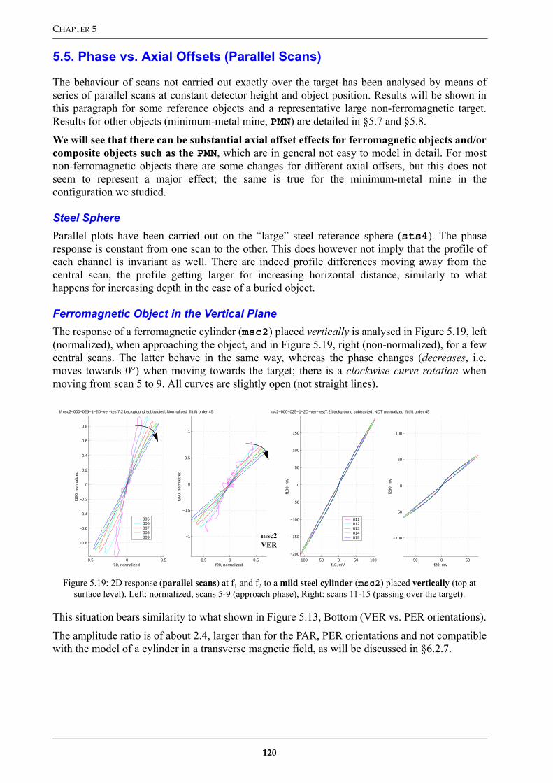
CHAPTER 5
5.5. Phase vs. Axial Offsets (Parallel Scans)
The behaviour of scans not carried out exactly over the target has been analysed by means ofseries of parallel scans at constant detector height and object position. Results will be shown inthis paragraph for some reference objects and a representative large non-ferromagnetic target.Results for other objects (minimum-metal mine, PMN) are detailed in §5.7 and §5.8.
We will see that there can be substantial axial offset effects for ferromagnetic objects and/orcomposite objects such as the PMN, which are in general not easy to model in detail. For mostnon-ferromagnetic objects there are some changes for different axial offsets, but this does notseem to represent a major effect; the same is true for the minimum-metal mine in theconfiguration we studied.
Steel SphereParallel plots have been carried out on the “large” steel reference sphere (sts4). The phaseresponse is constant from one scan to the other. This does however not imply that the profile ofeach channel is invariant as well. There are indeed profile differences moving away from thecentral scan, the profile getting larger for increasing horizontal distance, similarly to whathappens for increasing depth in the case of a buried object.
Ferromagnetic Object in the Vertical PlaneThe response of a ferromagnetic cylinder (msc2) placed vertically is analysed in Figure 5.19, left(normalized), when approaching the object, and in Figure 5.19, right (non-normalized), for a fewcentral scans. The latter behave in the same way, whereas the phase changes (decreases, i.e.moves towards 0°) when moving towards the target; there is a clockwise curve rotation whenmoving from scan 5 to 9. All curves are slightly open (not straight lines).
This situation bears similarity to what shown in Figure 5.13, Bottom (VER vs. PER orientations).
The amplitude ratio is of about 2.4, larger than for the PAR, PER orientations and not compatiblewith the model of a cylinder in a transverse magnetic field, as will be discussed in §6.2.7.
Figure 5.19: 2D response (parallel scans) at f1 and f2 to a mild steel cylinder (msc2) placed vertically (top at surface level). Left: normalized, scans 5-9 (approach phase), Right: scans 11-15 (passing over the target).
−0.5 0 0.5
−0.8
−0.6
−0.4
−0.2
0
0.2
0.4
0.6
0.8
f10, normalized
f190
, nor
mal
ized
B5/msc2−000−025−1−2D−ver−test7.2 background subtracted, Normalized filtfilt order 45
005006007008009
−0.5 0 0.5
−1
−0.5
0
0.5
1
f20, normalized
f290
, nor
mal
ized
−100 −50 0 50 100
−200
−150
−100
−50
0
50
100
150
f10, mV
f190
, mV
/msc2−000−025−1−2D−ver−test7.2 background subtracted, NOT normalized filtfilt order 45
011012013014015
−50 0 50
−100
−50
0
50
100
f20, mV
f290
, mV
msc2VER
120

MD RAW DATA ANALYSIS
Ferromagnetic Object in the Horizontal PlanePerpendicular orientation (PER): the response curves are nearly straight lines in the phase plane,but the phase changes from one scan to the other (see Figure 5.20)! The phase increases, i.e.moves towards +90°, when moving towards the target – counter clockwise curve rotation whenmoving from scan 5 to 9 – and is maximum over the object. Scan 12 features the maximum phase,and the minimum amplitude (in the object’s proximity obviously): lateral scans have a higheramplitude, contrary to standard scenarios. This is probably again a consequence of end effects(magnetic depolarisation). The PER phase response does therefore also change with axial offset.
Note that this behaviour is the opposite of what just discussed for the vertical orientation.
Parallel orientation (PAR): the response curves are “figure 8” shaped as expected (see Figure5.21), and the amplitude seems to have a “normal” behaviour (maximum for central scan). Thecurves are similar in close proximity to the object and change when moving away from it, but lessthan in the PER case. The non-symmetric behaviour is possibly due to some misalignment.
Figure 5.20: 2D response (parallel scans) at f1 and f2 to a mild steel cylinder (msc2) placed PERpendicularly (HOR plane). Left: normalized, scans 5-9 (approach phase), Right: scans 11-15 (passing over the target).
Figure 5.21: 2D response (parallel scans) at f1 and f2 to a mild steel cylinder (msc2) placed PARallel (HOR plane). Left: normalized, scans 5-9 (approach phase), Right: scans 11-15 (passing over the target).
−50 0 50
−100
−80
−60
−40
−20
0
20
40
60
80
100
f10, mV
f190
, mV
/msc2−000−025−1−2D−per−test7.2 background subtracted, NOT normalized filtfilt order 45
011012013014015
−40 −20 0 20
−60
−40
−20
0
20
40
60
f20, mV
f290
, mV
−0.4 −0.2 0 0.2 0.4
−0.8
−0.6
−0.4
−0.2
0
0.2
0.4
0.6
0.8
f10, normalized
f190
, nor
mal
ized
B5/msc2−000−025−1−2D−per−test7.2 background subtracted, Normalized filtfilt order 45
005006007008009
−0.5 0 0.5
−1
−0.5
0
0.5
1
f20, normalized
f290
, nor
mal
ized
msc2PER
−50 0 50−150
−100
−50
0
50
100
f10, mV
f190
, mV
/msc2−000−025−1−2D−par−test7.2 background subtracted, NOT normalized filtfilt order 45
011012013014015
−40 −20 0 20 40
−80
−60
−40
−20
0
20
40
60
80
f20, mV
f290
, mV
−0.4 −0.2 0 0.2
−0.8
−0.6
−0.4
−0.2
0
0.2
0.4
0.6
f10, normalized
f190
, nor
mal
ized
B5/msc2−000−025−1−2D−par−test7.2 background subtracted, Normalized filtfilt order 45
005006007008009
−0.6 −0.4 −0.2 0 0.2 0.4
−1
−0.8
−0.6
−0.4
−0.2
0
0.2
0.4
0.6
0.8
f20, normalized
f290
, nor
mal
ized
msc2PAR
121

CHAPTER 5
Non-Ferromagnetic Object in the Vertical PlaneThe response of a non-ferromagnetic cylinder (alc2) placed vertically is analysed in Figure 5.22(left, normalized) for a few central scans. The phase responses are practically unchanged,although some slight variations are not excluded far from the object. There is a slight opening ofthe curve(s), which does not happen with the PAR and PER configurations; it might be due to atilting of the cylinder’s axis.
Note again that same phase does not mean that the individual channels’ response profiles arespatially identical.Non-Ferromagnetic Object in the Horizontal PlanePerpendicular and Parallel orientation (PER, PAR): the phases are practically unchanged (seefor example Figure 5.22, right), although a slight increase is not excluded when moving from thecentre towards the edges – the phase seems to increase, i.e. moves towards 0° (from negativevalues), very slightly (a few degrees maximum).
Large Non-ferromagnetic ObjectIn Figure 5.23 the target object is the large and irregularly shaped piece of copper alreadyencountered. Within each scan there are some changes in the phase response, especially at f1,which could be due to the object’s irregular shape and/or higher order multipole terms; it wouldnevertheless still be easy to define an “average phase”. From one scan to the other there are noremarkable differences, apart from the response at f1 for D–12cm (scan 8, at the outer edges of theobject) which features also a reduced absolute value.
Figure 5.22: 2D response (parallel scans) at f1 and f2 to an aluminium cylinder (alc2). Left: placed vertically (top at surface level); normalized, scans 11-15 (passing over the target). Right: placed PERpendicularly (HOR plane);
normalized, scans 9-14 (passing over the target).
−0.5 0 0.5
−1
−0.5
0
0.5
1
f10, normalized
f190
, nor
mal
ized
b5/alc2−000−025−1−2D−ver−test7.3 background subtracted, Normalized filtfilt order 60
011012013014015
−0.5 0 0.5
−0.8
−0.6
−0.4
−0.2
0
0.2
0.4
0.6
0.8
f20, normalized
f290
, nor
mal
ized
−0.5 0 0.5
−1
−0.5
0
0.5
1
f10, normalized
f190
, nor
mal
ized
b5/alc2−000−025−1−2D−per−test7.3 background subtracted, Normalized filtfilt order 60
009010011012013014
−0.5 0 0.5
−0.8
−0.6
−0.4
−0.2
0
0.2
0.4
0.6
0.8
f20, normalized
f290
, nor
mal
ized
122

MD RAW DATA ANALYSIS
Figure 5.23: Response at f1 and f2 to a large copper debris, for four parallel scans at increasing axial offset from the object.
−400 −200 0 200 400
−300
−200
−100
0
100
200
300
f1 IM
AG
(m
Vol
t), f
2 IM
AG
(m
Vol
t)
Parallel scans over a large non−ferromagnetic object
f1f2
−200 0 200
−200
−100
0
100
200
300D − 4cm (scan 12)
f1f2
−100 0 100
−100
−50
0
50
100
150
f1 REAL (mVolt), f2 REAL (mVolt)
f1 IM
AG
(m
Vol
t), f
2 IM
AG
(m
Vol
t)
D − 8cm (scan 10)
f1f2
−50 0 50
−20
0
20
40
f1 REAL (mVolt), f2 REAL (mVolt)
D − 12cm (scan 8)
f1f2
123

CHAPTER 5
5.6. Phase vs. Orientation in the Horizontal Plane
We will analyse in this paragraph how the target’s response depends on its orientation in thehorizontal plane, the plane into which the metal detector moves.
Non-ferromagnetic CylindersNon-ferromagnetic cylinders, e.g. of aluminium or copper, do not show any noticeabledifference (see also previous discussion for coc2 in §5.3).
Ferromagnetic CylindersThe non-normalized response of a ferromagnetic cylinder (msc2) is shown in Figure 5.24 atfixed heights for each of the four orientations in the HORizontal plane (PAR, PER, QU1, QU4).The response is strongly orientation dependent. At f1 the PAR orientation features the largestamplitude, PER the smallest. The PAR profile is “figure 8” shaped, PER linear, QU1 and QU4intermediate. The behaviour at f2 is similar, but the “figure 8” curves are more regularly shaped(symmetric).
The curves for the smaller cylinder (msc1) show similar trends, with an even more markeddifference between the PAR and PER configurations.
There is in fact is not a large difference between the parallel configurations for msc1 and msc2,especially at f1 (the straight section in particular is the same; compare Figure 5.17 and Figure5.18). Probable explanation: the length, which is the same for msc1 and msc2 (only the cylinderdiameter changes), is the dominant factor, and with it the magnetic depolarisation effects. Thisseems consistent with the data in [BRA01].
Ferromagnetic Cylinders: Individual Channel ProfilesIndividual profiles are shown in Figure 5.25, with the figures not being always symmetric,possibly due to a non perfect positioning of the object59.
The shape of the real and the imaginary part curves (f1 and f2 REAL and IMAG) is notnecessarily the same any more, with the real part which seems to be the more irregular one; thereare also parts of the curves in which the two have opposite polarity, corresponding to a negativephase. The peaks do also not necessarily occur at the same spatial position. A closer look at thecurves shows that it is the central section between the first and last peak which exhibits thegreatest variation; the phase is rather constant to the left and to the right of it, i.e. whileapproaching the object and while moving away from it (not when over it). Similar plots are in factwell known in Non-Destructive Testing applications.
This behaviour can be explained qualitatively as follows60, thinking of the situation in which thecylinder is parallel (longitudinal) to the scanning direction: far away from the coil it sees basicallya horizontal primary magnetic field aligned along its axis, which emphasizes inducedmagnetization effects (and possibly increases µr). The object’s ferromagnetic nature prevails.Right over the coil the primary magnetic field is vertical and therefore transversal to the cylinderaxis; eddy current effects can prevail and the object can appear to behave as non-ferromagnetic.The field orientation effect is well illustrated in [END98, SOW99].
59. This measurement set is different from the previously shown ones; the curves are therefore not identical.60. K. Ausländer, Institut Dr. Förster, Private Communication, March 2000.
124
MD RAW DATA ANALYSIS
Figure 5.24: Response at f1 and f2 to a mild steel cylinder (msc2) placed flush with the surface, at fixed heights for each of the four orientations in the horizontal plane.
−200 −100 0 100 200
−200
−150
−100
−50
0
50
100
150
msc2 Test 7.2.1 h=025 f1
f10, mV
f190
, mV
parperqu1qu4
−50 0 50−60
−40
−20
0
20
40
msc2 Test 7.2.1 h=050 f1
f10, mV
f190
, mV
−5 0 5
−6
−4
−2
0
2
4
msc2 Test 7.2.1 h=100 f1
f10, mV
f190
, mV
−100 −50 0 50 100
−50
0
50
msc2 Test 7.2.1 h=025 f2
f10, mV
f190
, mV
parperqu1qu4
−20 0 20
−20
−10
0
10
20
msc2 Test 7.2.1 h=050 f2
f20, mV
f290
, mV
−4 −2 0 2−3
−2
−1
0
1
2
msc2 Test 7.2.1 h=100 f2
f20, mV
f290
, mV
125

CHAPTER 5
Figure 5.25: Response at f1 and f2 to a mild steel cylinder (msc2, flush), at four different orientations in the horizontal plane (parallel and orthogonal to the scanning direction, and at +45 and –45 degrees to it).
200 400 600 800
−100
−50
0
50
100
150
f1&
f2 R
EA
L,IM
AG
(m
Vol
t)
Parallel to scanning direction (−> x)
f1f2
−100 0 100−100
−50
0
50
100
150
f1 IM
AG
(m
Vol
t), f
2 IM
AG
(m
Vol
t)
complex plane representation
f1f2
200 400 600 800−100
−50
0
50
100
f1&
f2 R
EA
L,IM
AG
(m
Vol
t)
Perpendicular to scanning direction (−> y)
f1f2
−100 −50 0 50
−50
0
50
f1 IM
AG
(m
Vol
t), f
2 IM
AG
(m
Vol
t)
f1f2
Ferromagneticobject (ex. mildsteel cylinder)
200 400 600 800−100
−50
0
50
100
150
f1&
f2 R
EA
L,IM
AG
(m
Vol
t)
At +45 degrees (−> y=x)
f1f2
−100 −50 0 50 100 150
−50
0
50
100
f1 IM
AG
(m
Vol
t), f
2 IM
AG
(m
Vol
t)
f1f2
200 400 600 800
−100
−50
0
50
100
f1&
f2 R
EA
L,IM
AG
(m
Vol
t)
At −45 degrees (−> y=−x)
f1f2
−100 −50 0 50 100−100
−50
0
50
100
f1 IM
AG
(m
Vol
t), f
2 IM
AG
(m
Vol
t)
f1f2
126

MD RAW DATA ANALYSIS
5.7. Response for a Minimum-metal Mine and its Components
We will analyse in the following the response of a minimum-metal mine and of its components.Although this particular type of mine is not widely diffused, it is still representative of thecategory, and will allow to draw a number of interesting conclusions.
Complete Live (i.e. real) MineFigure 5.26 features the response of the live (real) minimum-metal mine (mich) shown to theright of Figure 5.4 – i.e. of a composite object – and of its metallic components separately, thesmall steel striker pin, mist, and the real detonator, midereal.
It is very interesting to see that the detonator, which is actually just above the striker pin andtherefore slightly closer to the detector, delivers a significant and absolutely not negligible signal,non-ferromagnetic in nature (perhaps due to the thin capsule containing the primary explosive)with an f2 component much larger than the f1 component. This would indeed be indicative,according to the models of Chapter 3, of a rather small object. It is in any case a reminder toinclude whenever possible the detonator, or equivalent metallic pieces, in the study of minimum-metal mines.
The signal of the mine without detonator is on the other hand of ferromagnetic nature, the minecontaining in this case only the steel striker pin already analysed in a number of plots (actually avertically placed steel nail, of diameter 1.5 mm, length 11 mm and weight 0.1-0.2 g).
The signal of the real complete (live) mine is an interesting combination of the two – actuallysimply the vector sum of the first two plots – looking like the response of a ferromagnetic objectat f1 and of a non-ferromagnetic one at f2; this seems quite characteristic indeed. All scans werecarried out on flush objects with a detector height of 5 cm. The live mine was also scanned at adetector height of 10 cm, and the corresponding responses look quite similar to those at 5 cm.
Figure 5.26: Minimum-metal mine: response to a detonator cap (midereal), to the mine without detonator, i.e. striker pin only (mist), and to the live (real) mine (mich) at two different detector heights (all objects flush)
[BRU00b]. EPFL data, taken with the assistance of the Swiss Defence Procurement Agency.
−10 −5 0 5
−6
−4
−2
0
2
4
6
f1 IM
AG
(m
Vol
t), f
2 IM
AG
(m
Vol
t)
Detonator only
f1f2
−5 0 5
−4
−2
0
2
4
Mine without Detonator
f1f2
−5 0 5
−6
−4
−2
0
2
4
6
f1 REAL (mVolt), f2 REAL (mVolt)
f1 IM
AG
(m
Vol
t), f
2 IM
AG
(m
Vol
t)
Live Mine, MD @ 5cm
f1f2
−1 −0.5 0 0.5 1
−0.5
0
0.5
1
f1 REAL (mVolt), f2 REAL (mVolt)
Live Mine, MD @ 10cm
f1f2
127

CHAPTER 5
Mine Striker Pin at Increasing DistanceFigure 5.27 represents the response to the striker pin only (mist), placed vertically. The detectorhead was raised in 2 cm increments, without displacing the object. The plots at a distance of 3 cmcorrespond in fact to the signals shown in Figure 5.3 and Figure 5.5.
The phase of the object seems to stay constant in this case too, but it is difficult to make precisestatements because of the varying background signal (the f2 component in particular is stronglyperturbed). These, together with the actual form of the object, long and slender and therefore farfrom resembling a sphere, and/or its placement (vertical), might explain why the phase angle ismuch smaller than one would expect for such a small object. These plots do also represent a goodexample of unfavourable signal to noise ratio.
Comparison of Striker PinsDifferent versions of the striker pin described above (mist1,2,3 – inert mine components)have been compared among them and with the striker of the real mine tested at the EPFL; the pinswere placed vertically (usual configuration). No differences were detected.
Measurements were also carried out with the striker pin in the horizontal plane, parallel (PAR)and perpendicular (PER) to the scanning direction. This corresponds to an unusual placement ofthe mine, which however can not be totally excluded a priori, either due to natural events or to adeliberate act. An instance of the latter was for example recorded in the Sarajevo area a few yearsago, when a deminer hit the pressure plate of a vertically placed mine while prodding.
Figure 5.27: Response at f1 and f2 to a small striker pin (mist) contained in a minimum-metal mine placed flush with the surface, for increasing detector heights
−40 −20 0 20 400
10
20
30
40
Small striker pin (min. metal mine), Dist = 1cm
f1&
f2 IM
AG
(m
Vol
t) f1f2
−10 0 10
0
5
10
15
Distance = 3cm
f1f2
−5 0 5−2
0
2
4
6
Distance = 5cm
f1&
f2 IM
AG
(m
Vol
t) f1f2
−2 0 2
0
1
2
3
Distance = 7cm
f1f2
−2 −1 0 1
0
0.5
1
1.5
Distance = 9cm
f1 REAL (mVolt), f2 REAL (mVolt)
f1&
f2 IM
AG
(m
Vol
t) f1f2
−0.5 0 0.5
0
0.2
0.4
0.6
Distance = 11cm
f1 REAL (mVolt), f2 REAL (mVolt)
f1f2
128
MD RAW DATA ANALYSIS
The resulting behaviour, shown in Figure 5.28, is quite similar to what previously described forthe larger steel cylinder (msc2) in §5.3 (see Figure 5.13). Note in particular the differencebetween the VER and PER orientations. The signal amplitudes are in the following order: VER(Delta~5 mV), PAR (Delta~2 mV), PER (Delta<0.5 mV, barely detected at s=2). In the PARorientation the individual channels exhibit multiple peaks.
The overall mine response would obviously include the contribution from the detonator as well.
Figure 5.28: Minimum-metal mine striker pin (mist1): response to different orientations. Top: VER vs. PAR, Bottom: VER vs. PER. Normalized.
−2.5 −2 −1.5 −1 −0.5 0 0.5 1 1.5 2 2.5
−0.5
0
0.5
f10f1
90
measvub6/mist1−flu−025−1−ver.001 vs measvub6/mist1−flu−025−2−par.001 (BGND subtracted and normalized)
f1 first filef1 second file
−2.5 −2 −1.5 −1 −0.5 0 0.5 1 1.5 2 2.5
−0.5
0
0.5
f20
f290
f2 first filef2 second file
−2.5 −2 −1.5 −1 −0.5 0 0.5 1 1.5 2 2.5
−0.5
0
0.5
f10
f190
measvub6/mist1−flu−025−1−ver.001 vs measvub6/mist1−flu−025−2−per.001 (BGND subtracted and normalized)
f1 first filef1 second file
−2.5 −2 −1.5 −1 −0.5 0 0.5 1 1.5 2 2.5
−0.5
0
0.5
f20
f290
f2 first filef2 second file
VER vs. PAR
VER vs. PER
VER
PER
129

CHAPTER 5
Comparison of Mine DetonatorsComparison with real detonator: A replica detonator (mide) (essentially composed of acylindrical foil), provided by the Swiss Defence Procurement Agency, was compared to theoriginal detonator of the real mine tested at the EPFL61 (midereal). The behaviour is similarbut the phases are not identical (Figure 5.29, left); the replica detonator does therefore represent agood but not perfect reproduction. The actual angle at f1, which is quite small, is in fact slightlylower than what shown due to important background effects.
The background subtracted profile is visible in Figure 5.29, right; this is also a reminder of theimportance of soil effects, in particular for small objects/weak signals. As already notedelsewhere the response at f1 is much weaker than at f2. The amplitude ratio is about 1/6,characteristic of a quite small and/or poorly conductive non-ferromagnetic object.
Comparison at different heights: The response was checked at a height of 2.5, 5, 10 and 15 cm. Itdoes not change at least up to 10 cm, although it is quite weak at f1. At 15 cm the target is barelydetectable at s=3.
Comparison of different orientations (VER vs PER, PAR): no changes in phase response areapparent, and in this case background subtraction works quite well as shown in Figure 5.29, right.
“Upside down” MineA complete mine was placed “upside down”, i.e. with the striker above the detonator, as well ason its side. The response is quite different from the standard one, the striker pin prevailing in thefirst case (closer to the coil).
This is a good example of problems due to composite objects, which can probably not bedescribed with one of the models discussed in Chapter 3.
Axial Offsets (Parallel Scans)In Figure 5.30 the target is again the real (live) version (real detonator). The distance between thescans plotted is 4 cm, with the scan running directly over the object being in between the secondand third (in fact between scan 13 and scan 14, which is 2 cm to the right of scan 13). There aresome changes in the phase at f2 and the ratio of the absolute values of the induced voltages at f1and f2 is not constant, in particular for the last scan shown (C+7cm, scan 17).
61. Live detonators are not easily available for tests due to the presence of very sensitive primary explosives.
Figure 5.29: Minimum-metal mine detonators: Left: replica (mide) vs. original one (midereal, shown in Figure 5.4); normalized. Right: replica (mide) response to different orientations, VER vs. PAR; normalized, background
subtracted.
−1 −0.8 −0.6 −0.4 −0.2 0 0.2 0.4 0.6 0.8 1
−0.3
−0.2
−0.1
0
0.1
0.2
0.3
f10
f190
measvub6/mide−000−025−1−ver−test7.6.001 vs minech2dreal/mli11b.014 (mean subtracted and normalized)
f1 first filef1 second file
−2.5 −2 −1.5 −1 −0.5 0 0.5 1 1.5 2
−0.5
0
0.5
f20
f290
f2 first filef2 second file
−0.8 −0.6 −0.4 −0.2 0 0.2 0.4 0.6 0.8
−0.2
−0.1
0
0.1
0.2
0.3
f10
f190
measvub6/mide−000−025−1−ver−test7.6.001 vs measvub6/mide−000−025−1−par−test7.6.001 (BGND subtracted a
f1 first filef1 second file
−2 −1.5 −1 −0.5 0 0.5 1 1.5 2
−0.6
−0.4
−0.2
0
0.2
0.4
0.6
f20
f290
f2 first filef2 second file
130

MD RAW DATA ANALYSIS
Figure 5.30: Response at f1 and f2 to a minimum-metal live mine (flush), for four parallel scans (the scan running directly over the object being in between the second and third) [BRU00b].
−5 0 5−5
0
5
f1 IM
AG
(m
Vol
t), f
2 IM
AG
(m
Vol
t)
Parallel scans over a live minimum metal mine
C − 5cm (scan 11)
f1f2
−5 0 5
−6
−4
−2
0
2
4
6
C − 1cm (scan 13)
f1f2
−5 0 5
−6
−4
−2
0
2
4
6
f1 REAL (mVolt), f2 REAL (mVolt)
f1 IM
AG
(m
Vol
t), f
2 IM
AG
(m
Vol
t)
C + 3cm (scan 15)
f1f2
−5 0 5
−4
−2
0
2
4
f1 REAL (mVolt), f2 REAL (mVolt)
C + 7cm (scan 17)
f1f2
131

CHAPTER 5
5.8. Response for a PMN mine
We will analyse in the following the response of the Russian PMN, a widely diffused nonminimum-metal AP mine (see Figure 5.4).
5.8.1. Phase vs. Distance (depth)PMN data was collected at the VUB sandbox with the mine at different depths (5, 10, 20, 26 cmto top of mine) using a PVC cylinder to ease data taking. Scans were first taken with the emptytube (BGND), then the empty tube with the mine placed as in Figure 5.31 (“emptyhole”), andfinally the tube containing the mine and filled with sand (“fillhole”), corresponding to a realisticsetup of a buried mine. This starting from the deepest position, moving upwards from onesequence to the next.
The PMN used in these tests (pmnVUB, similar to the one in Figure 5.4) featured theferromagnetic cover retaining ring; it was not yet armed (the arming pin was still in place, the ringusually attached to it had however been removed).
We will concentrate here on the data of the “emptyhole” scans, background subtracted to obtainthe response from the mine alone. Results are shown in Figure 5.32, which compares the responseat 5 cm with the one at 10 cm and 20 cm.
The phase seems clearly non-ferromagnetic at f2 (eddy current effects prevail), a superposition atf1. The straight section at f1 (with negative slope) does probably correspond to the ring, andshould correspond to the response right above the mine. As from 20 cm there are appreciabledifferences due to the soil (in the tube). Background subtraction seems however not to be efficientenough for a clear soil effect cancellation; the data at a depth of 26 cm is therefore quite irregular.
Some phase response differences with depth are clearly visible.
5.8.2. Phase vs. Axial Offsets (Parallel Scans) and Orientation in the HORPlaneFour different orientations were analysed in the horizontal plane, namely PAR1 (as in Figure5.31) followed by 3 successive counter clockwise rotations: PER1, PAR2 and PER2. Thirteen 2Dscans were carried out at a pitch of 4 cm instead of the usual 26 scans at a pitch of 2 cm.
Figure 5.31: Setup for the measurement of a PMN mine at the VUB sandbox (see text).
132

MD RAW DATA ANALYSIS
The data corresponding to the PAR1 configuration is shown in Figure 5.33. The target lookstypically ferromagnetic at large distances (scan 3 for example); the response “rotates” thentowards the response above the target62, scan 7, which is in fact the one already shown in Figure5.32.
Very important phase response differences with axial offset are clearly visible.
Comparison of different orientations in the horizontal plane: PAR1 and PER1, PAR2 and PER2,look similar although they are not identical as clearly shown in Figure 5.34, in particular far fromthe object (approaching and moving away). Note that the PAR2 and PER2 responses go throughthe origin at f1, whereas PAR1 and PER1 are vertically offset. The amplitude of the response at f2is much larger than at f1.
Figure 5.32: pmnVUB response, complete mine at different depths, 1D scan over the mine; depth=5 cm vs. 10 cm (Top) and 5 cm vs. 20 cm (Bottom). Normalized.
62. The maximum is actually between scans 7 and 8.
−1.5 −1 −0.5 0 0.5 1 1.5−0.6
−0.4
−0.2
0
0.2
0.4
f10
f190
svub6/pmnVUB−050−025−1−par1−emptyhole.001 vs measvub6/pmnVUB−100−025−1−par1−emptyhole.001 (BGND subtracted and n
f1 first filef1 second file
−2 −1.5 −1 −0.5 0 0.5 1 1.5 2
−0.6
−0.4
−0.2
0
0.2
0.4
0.6
f20
f290
f2 first filef2 second file
−1.5 −1 −0.5 0 0.5 1 1.5
−0.6
−0.4
−0.2
0
0.2
0.4
f10
f190
svub6/pmnVUB−050−025−1−par1−emptyhole.001 vs measvub6/pmnVUB−200−025−1−par1−emptyhole.001 (BGND subtracted and n
f1 first filef1 second file
−2 −1.5 −1 −0.5 0 0.5 1 1.5 2
−0.6
−0.4
−0.2
0
0.2
0.4
0.6
f20
f290
f2 first filef2 second file
133

CHAPTER 5
Figure 5.33: 2D response (parallel scans) at f1 and f2 for pmnVUB, placed at PAR1 (HOR plane). Normalized, scans 3-7 (approaching the target; centre of target between scans 7 and 8), 4 cm increments.
Figure 5.34: Comparison of the response at f1 and f2 over pmnVUB, for 4 orientations in the HOR plane; scan 7 (above the target).
−0.5 0 0.5
−1.5
−1
−0.5
0
0.5
1
1.5
f10, normalized
f190
, nor
mal
ized
6/pmnVUB−000−025−1−par1−2D NOT background subtracted, Normalized filtfilt order 45
003004005006007
−0.5 0 0.5−1.5
−1
−0.5
0
0.5
1
1.5
f20, normalizedf2
90, n
orm
aliz
ed
−500 0 500
−1500
−1000
−500
0
500
1000
1500
pmnVUB Test 7.4.2 scan 7 f1
f10, mV
f190
, mV
PAR1PAR2PER1PER2
−1000 0 1000
−3000
−2000
−1000
0
1000
2000
3000
pmnVUB Test 7.4.2 scan 7 f2
f10, mV
f190
, mV
PAR1PAR2PER1PER2
134

MD RAW DATA ANALYSIS
5.8.3. Response for Different Versions of a PMN mine
Mine StrikerA PMN replica version was initially obtained from MILTRA Engineering in the UK. This replicamine contains a steel striker, believed to be an exact copy of the original, composed of twocylinders aligned along the same axis, with diameter 9 mm and 5 mm and length 19 mm and 39mm respectively. This is the mine’s largest metallic object apart from the ferromagnetic coverretaining ring, also visible in Figure 5.4.
The phase response to this steel striker is strongly orientation dependent, given that it iscomposed of two coaxial steel cylinders and that it is ferromagnetic.
Later on we also had access to a mine, coming from Cambodia (pmnCambodia), which lookedvery much like a PMN but which turned out to have a slightly smaller non-ferromagnetic (!)striker pin, possibly made of an alloy. This is in fact the mine actually shown in Figure 5.4 to theleft. The response to its striker pin is displayed in Figure 5.35, and is obviously very different tothe one of the replica version. The mine could be a Chinese copy of the PMN, but this episodewas actually very useful in reminding us of the limits of a target identification based approach.
Complete MineThe complete pmnCambodia mine was analysed for the different orientations in the HOR plane.The results are qualitatively similar to those of pmnVUB, however not identical (the response at f2over the mine depends for instance on its orientation). This could be due to some differences inthe components and/or in the mine setup (armed for pmnCambodia, unarmed for pmnVUB).This has again to be taken into account in a target identification based approach.
Figure 5.35: Response at f1 and f2 to a PMN “like” AP mine (pmnCambodia) non-ferromagnetic striker (flush), at four different orientations (parallel and orthogonal to the scanning direction, and at +45° and –45°).
−50 0 50
−60
−40
−20
0
20
40
60
f1 IM
AG
(m
Vol
t), f
2 IM
AG
(m
Vol
t)
Parallel to scanning direction (−> x)
f1f2
−50 0 50
−60
−40
−20
0
20
40
60
Perpendicular to scanning direction (−> y)
f1f2
−50 0 50
−60
−40
−20
0
20
40
60
f1 REAL (mVolt), f2 REAL (mVolt)
f1 IM
AG
(m
Vol
t), f
2 IM
AG
(m
Vol
t)
At +45 degrees (−> y=x)
f1f2
−50 0 50
−60
−40
−20
0
20
40
60
f1 REAL (mVolt), f2 REAL (mVolt)
At −45 degrees (−> y=−x)
f1f2
PMN "like" APnon−ferromagneticstriker
135

CHAPTER 5
5.9. Response for Metallic Mines and (composite) UXO
Metallic AP mines are usually designed to kill via fragmentation, up to some tens of meters, andare composed of a relevant mass of metal as well as of explosive. Examples of a boundingfragmentation mine and a stake fragmentation mine are shown in Figure 5.36. The first isdesigned to be buried, the second to placed on a (wooden) stake just above the surface.
Metallic mines are in principle easier to detect, often even visually. There are howevercircumstances in which the stake mine is found lying on the surface63 or even buried. In addition,if we are relying on a discriminative metal detector we must be sure that the signal from such atype of mine is not going to be rejected by error. We have therefore investigated the response ofthe previously mentioned mines, as reported below.
5.9.1. PROM – Bounding Fragmentation MineA cylindrically shaped PROM bounding fragmentation mine, whose steel body is about 20 cmlong, was buried vertically, with only the top (a pronged striker about 4 cm long) sticking abovethe soil, and acquisitions taken in 2D. The results are shown in Figure 5.37.
Note the phase response at f1, which is slightly negative above the mine and slightly positive farfrom it (scans 1-5, not shown). In order to avoid mistaking the mine for a (small) non-ferromagnetic object it could therefore be quite useful to:
• rely on a third lower frequency as well, or• impose a threshold on the signal amplitude above which any target is declared as suspicious
(which might anyhow be the case to cope with the problem of a small target close to a largerinnocuous object), or
Figure 5.36: Metallic mines. Left: PROM (bounding fragmentation), Right: PMR-2A (stake fragmentation; stake not shown). Origin: Ex-Yugoslavia. Ruler length: 20+2.5 cm.
63. In case the wooden stake breaks or rots for example.
136

MD RAW DATA ANALYSIS
• exploit the fact that the phase response curves are quite open, or• exploit the amplitude ratio information: AR is slightly <1 here, and therefore quite unlikely to
correspond to a small non-ferromagnetic object (see also §6.2.6).Incidentally, the overall amplitudes are not very large in this case, given the mass of the mine, andthey change only slightly over the mine.
Figure 5.37: 2D response (parallel scans) at f1 and f2 to a PROM mine placed vertically (pronged striker above surface). Top: normalized, scans 6-10 (approach phase), Bottom: scans 11-15 (passing over the target).
−0.5 0 0.5
−1.5
−1
−0.5
0
0.5
1
1.5
f10, normalized
f190
, nor
mal
ized
svub7/prom−200−050−1−ver NOT background subtracted, Normalized filtfilt order 45
006007008009010
−0.4 −0.2 0 0.2 0.4
−0.8
−0.6
−0.4
−0.2
0
0.2
0.4
0.6
0.8
f20, normalizedf2
90, n
orm
aliz
ed
−100 0 100
−300
−200
−100
0
100
200
300
f10, mV
f190
, mV
ub7/prom−200−050−1−ver NOT background subtracted, NOT normalized filtfilt order 45
011012013014015
−100 −50 0 50 100
−200
−150
−100
−50
0
50
100
150
200
f20, mV
f290
, mV
137
CHAPTER 5
5.9.2. PMR-2A – Stake Fragmentation MineVertical orientation: A cylindrically shaped PMR-2A stake fragmentation mine, also made ofsteel and overall about 20 cm long, was placed vertically above the ground, and acquisitionstaken in 2D.
The results, shown in Figure 5.38, represent a nice example of the response of a largeferromagnetic object, with a positive phase response at f1 and a largely negative one at f2, withopen curves (typical of ferromagnetic objects) and AR~1.3, and would allow an easy targetidentification. Note that the straight section does here correspond to the central part of the scan,above the object, when the magnetic field is mostly aligned along the mine’s axis of symmetry.Signal amplitudes are not very large in this example.
Perpendicular and Parallel orientation: Measurements were also carried out with a mine lyingon the surface (as if it had fallen down, see introductory remarks). Four different orientationswere analysed, namely PAR1 (parallel to the scanning direction and detector first scanning thepin, then the mine body) followed by 3 successive counter clockwise rotations: PER1, PAR2 andPER2. The detector output was unfortunately partially saturated due to the close proximity to themine.
The responses to the PER1 and PER2 orientations are nearly identical, PAR1 and PER2 aresimilar but not exactly equal. What is perhaps more important is that PAR and PER are moresimilar to each other than to the vertical orientation. Their phase response is rotated at bothfrequencies towards the vertical compared to the VER configuration (see also Figure 5.39); it ishowever still positive at f1 and negative at f2, with quite a large phase difference between the twovalues, and should therefore still be quite distinctive. This situation bears some similarity to theresults for the large reference cylinder (msc2), VER vs. PER configurations (see Figure 5.13).
Figure 5.38: 2D response (parallel scans) at f1 and f2 to a PMR-2A mine placed vertically (mine above surface). Scans 11-15 (passing over the target).
−150 −100 −50 0 50 100
−250
−200
−150
−100
−50
0
50
100
150
200
250
f10, mV
f190
, mV
7/pmr2−000−300−1−2d−ver NOT background subtracted, NOT normalized filtfilt order 45
011012013014015
−50 0 50
−100
−50
0
50
100
150
f20, mV
f290
, mV
138
MD RAW DATA ANALYSIS
5.9.3. A Composite UXO ExampleTests were also carried out with a 20 mm projectile shown in Figure 7.12, an interestingcomposite object about 14 cm long, featuring a non-ferromagnetic tip (likely aluminium) on topof a cylindrical steel body. The overall response can therefore be highly orientation-dependent,according to the strength of the responses of the two parts (the overall behaviour can probably beapproximated with the sum of two physically separated dipoles).
Vertical orientation: the target was placed vertically with the nose upwards (“up”) anddownwards (“down”), with the detector carrying out 1D scans at different heights (Figure 5.40,Top). The response is radically different for the two orientations, in particular at f2, due to the factthat in one case the non-ferromagnetic tip is closest to the object, in the other it is farthest. Theresponse is largest with the target pointing downwards; it depends here also on the height.
The response amplitude ratios are about 2.75 (down) and 2.1 (up) at a height of 2.5 cm, the firstvalue being typical of an elongated ferromagnetic object when the primary magnetic field ismostly aligned with its symmetry axis.
Perpendicular and Parallel orientations: Measurements were also carried out with the targetlying on the surface at four different orientations, PAR1 and PAR2, PER1 and PER2 (Figure 5.40,Bottom). The PAR1 and PAR2 responses are quite irregular and change somewhat with distance,whereas PER1 and PER2 are much more stable (straight lines), especially at f1. In this case theparallel orientation seems to deliver a less strong signal than the perpendicular one, contrary towhat we have seen for most other cylindrical ferromagnetic objects.
In spite of the response changes with orientation, the target can be clearly identified at allorientations as a large (mostly) ferromagnetic object.
Figure 5.39: Response at f1 and f2 to a PMR-2A mine at different orientations: VER vs. PER. Normalized.
−2 −1.5 −1 −0.5 0 0.5 1 1.5 2
−0.6
−0.4
−0.2
0
0.2
0.4
0.6
0.8
f10
f190
measvub7/pmr2−000−300−1−2d−ver.013 vs measvub7/pmr2−000−075−1−per1.001 (mean subtracted and normalized)
f1 first filef1 second file
−2 −1.5 −1 −0.5 0 0.5 1 1.5 2
−0.6
−0.4
−0.2
0
0.2
0.4
0.6
f20
f290
f2 first filef2 second file
139

CHAPTER 5
Figure 5.40: Response at f1 and f2 to a 20 mm projectile (bul1), flush. Top: vertical down and up, at two different detector heights (normalized); Bottom, horizontal at 4 different orientations (detector at 2.5 cm)
−1000 −500 0 500 1000
−1500
−1000
−500
0
500
1000
1500
f10, mV
f190
, mV
bul1 (200 mm proj.) HOR NOT normalized filtfilt order 45
PAR1 h025PAR2 h025PER1 h025PER2 h025
−1000 −500 0 500 1000−2000
−1500
−1000
−500
0
500
1000
1500
2000
f20, mV
f290
, mV
−0.5 0 0.5
−1.5
−1
−0.5
0
0.5
1
1.5
f10, normalized
f190
, nor
mal
ized
bul1 (200 mm proj.) VER Normalized filtfilt order 45
VER down h025VER up h025VER down h100VER up h100
−0.5 0 0.5
−1.5
−1
−0.5
0
0.5
1
1.5
f20, normalized
f290
, nor
mal
ized
140

MD RAW DATA ANALYSIS
5.10. Response for Other Mine Types
Figure 5.41 shows the response of a Vietnamese MD-82B AP mine (miviet), also collected inCambodia. This mine does visually look like a US M-14 AP; it does however contain differentmetal components – the fuzing system is completely different – and is “easily” detectable. In thissense it is not a minimum-metal mine. The response is clearly ferromagnetic and does not changewith distance for the scans carried out.
Figure 5.41: Response at f1 and f2 to a Vietnamese MD-82B AP mine (miviet), flush, at two different detector heights.
−1500 −1000 −500 0 500 1000 1500
−500
0
500
miviet ("Vietnamese mine") f1 f2 h=025 flush filtfilt order 45
mV
mV
h=025 f1h=025 f2
−80 −60 −40 −20 0 20 40 60 80
−20
−10
0
10
20
miviet ("Vietnamese mine") f1 f2 h=100 flush filtfilt order 45
mV
mV
h=100 f1h=100 f2
141

CHAPTER 5
5.11. Clutter (Debris) Analysis
During the tests carried out by the EPFL DeTeC team in Cambodia with a GPR prototype[BRO98], numerous metallic debris samples were collected from a simulated minefield situatednext to a village. Although inert mines had been emplaced, the Halo Trust team followed theirstandard operating procedures using an Ebinger Ebex 420 SI MD. Each metallic piece, or set ofpieces, was then removed and collected. The land was otherwise untreated; the collected cluttershould therefore be representative. Examples are provided in A5.5.
In the following we have tried to form groups of similar objects whenever possible. Note that allsizes in the following table are approximate.
Debris Group #1: deb01-16, 16 objects – Cylinders, PlatesThe objects in this group are listed in the following table:
They can be indicatively subdivided as follows (all are ferromagnetic except 14, 16):• Cylindrical objects (nails etc.; deb01-07). MD signals for the PAR orientation are usually quite
stronger than for PER. The responses (see Figure 5.42) bear qualitative similarity to the ones fromferromagnetic cylinders.
• Plates (deb08-10): the phase angles are closer to +90° than the previous cylindrical objects(Figure 5.43, Top).
ID Description Geometry Size (cm) Comments MD ResponseComments
01 Rusted nail CYL L:6 Ø:0.5
02 Rusted nail CYL L:5.5-6 Ø:0.5 Irregular Ø(strong)
03 Rusted cyl CYL L:7.5 Ø:0.3-0.4
04 Rusted nail (bent) CYL L:6 Ø:0.3-0.4 Bent in middle No straight line
05 Rusted nail CYL L:4 Ø:0.3-0.4 Irregular Ø(weak)
06 Rusted cyl CYL L:2.5 Ø:0.2-0.3
07 Rusted nail, bent linear L:3 Ø:0.2 Bent at 1cm Weak response
08 Plate RECT L,H: 2.5 “T” shaped, flat Irregular at f2
09 Plate RECT L,H: 2.5 “T” shaped, flat Irregular at f2
10 Plate “L” shaped L,H: 2 Outer dim.
11 Bottle cap ROUND Ø: 3 Earth covered Very odd!
12 Shrapnel IRREG L:3 H:2 Open curve, ferro
13 Shrapnel IRREG L:3 H:2 Ferro
14 Piece of hardplastic?
TRAPEZ L:3 H:3 Flat Non-ferro
15 Fragments IRREG Scattered, flat Magnetic, no MDalarm (s=3)
16 Rivet head ROUND Ø:0.8 H:0.3 short Weak response.Non-ferro
142

MD RAW DATA ANALYSIS
• Other: deb11 has a quite irregular behaviour; deb14 and deb16 are typically non-ferromagnetic; deb15 are magnetic fragments (Figure 5.43, Bottom).
deb15 represents a type of target, usually magnetic with a clear imaginary signal (a few mV), towhich the Förster MD does not react with an alarm. This might be due to the fact that on the fielda different MD has been used, which might be sensitive to (purely) magnetic objects, and/or thatsuch objects were close to a normal (conductive) target.
Figure 5.42: Response at f1 and f2 to deb01-07 in the horizontal plane; normalized, objects on the surface. Top: PER, Bottom: PAR.
−0.5 0 0.5−1
−0.8
−0.6
−0.4
−0.2
0
0.2
0.4
0.6
0.8
1
f10, normalized
f190
, nor
mal
ized
debris−list01−07par NOT background subtracted, Normalized filtfilt order 45
deb01deb02deb03deb04deb05deb06deb07
−0.4 −0.2 0 0.2 0.4 0.6
−1
−0.8
−0.6
−0.4
−0.2
0
0.2
0.4
0.6
0.8
1
f20, normalized
f290
, nor
mal
ized
−0.4 −0.2 0 0.2 0.4
−0.8
−0.6
−0.4
−0.2
0
0.2
0.4
0.6
0.8
f10, normalized
f190
, nor
mal
ized
debris−list01−07per NOT background subtracted, Normalized filtfilt order 45
deb01deb02deb03deb04deb05deb06deb07
−0.4 −0.2 0 0.2 0.4
−0.8
−0.6
−0.4
−0.2
0
0.2
0.4
0.6
0.8
f20, normalized
f290
, nor
mal
ized
143

CHAPTER 5
Figure 5.43: Response at f1 and f2 to deb08-10&12-13 (Top) and deb11&14-16 (Bottom) in the horizontal plane; normalized, objects on the surface.
−0.4 −0.2 0 0.2 0.4
−0.8
−0.6
−0.4
−0.2
0
0.2
0.4
0.6
0.8
f10, normalized
f190
, nor
mal
ized
debris−list08−13 NOT background subtracted, Normalized filtfilt order 45deb08−000−025−1−T.001deb09−000−025−1−T.001deb10−000−025−1−L.001deb12−000−025−1.001deb13−000−025−1.001
−0.6 −0.4 −0.2 0 0.2 0.4
−1
−0.8
−0.6
−0.4
−0.2
0
0.2
0.4
0.6
0.8
1
f20, normalized
f290
, nor
mal
ized
−0.5 0 0.5
−1.5
−1
−0.5
0
0.5
1
1.5
f10, normalized
f190
, nor
mal
ized
debris−list11−14−16 NOT background subtracted, Normalized filtfilt order 45
deb11deb14deb15deb16
−0.5 0 0.5
−1.5
−1
−0.5
0
0.5
1
1.5
f20, normalized
f290
, nor
mal
ized
144

MD RAW DATA ANALYSIS
Debris Group #2: deb20-26, 7 objects – Non-Ferromagnetic FoilsObjects in this group are non-ferromagnetic foils:
Their main characteristics are (see Figure 5.44):• The responses are mostly quite weak, especially at f1; actually: AR~1/7-1/8.• All phase are close to 0°, excepted deb20 (see Figure 5.44).
Note that plotting the phase difference would give a very low value for all objects (excepteddeb20), resulting in good discrimination. In this case discriminating on the amplitude ratioshould also work well.
ID Description Geometry Size (cm) Comments MD ResponseComments
20 Large foil RECT L,H: 10 irregular Strong response
21 Foil RECT L: 6 H: 2 irregular
22 Foil RECT L: 3 H: 1.5
23 Small foil RECT L: 1.5 H: 2
24 Small foil RECT L: 3 H: 1
25 Foil pieces RECT L,H: 1 (max) 7 pieces
26 Foil pieces RECT L:2 H:1 (max) 8 pieces
Figure 5.44: Response at f1 and f2 to deb20-26 in the horizontal plane; normalized, objects on the surface.
−0.5 0 0.5
−1.5
−1
−0.5
0
0.5
1
1.5
f10, normalized
f190
, nor
mal
ized
debris−list20−26 background subtracted, Normalized filtfilt order 75
deb20deb21deb22deb23deb24deb25deb26
−0.5 0 0.5
−1.5
−1
−0.5
0
0.5
1
1.5
f20, normalized
f290
, nor
mal
ized
145

CHAPTER 5
Debris Group #3: deb30-39, 10 objects – Ferromag. Foils and Small FragmentsObjects in this group are ferromagnetic foils and collections of small fragments thereof:
Their main characteristics are (Figure 5.45):• Their phase responses are quite close to +90° (excepted deb31, a large object, and deb35).• Some of them give small phase difference (and sometimes, when the amplitudes at f1 and f2 are
quite close, small amplitude difference values as well). This could again be used as adiscrimination criterion.
ID Description Geometry Size (cm) Comments MD ResponseComments
30 Rusted RECT L,H: 4 ferro
31 Rusted RECT L,H: 6 Large irregular Open curve
32 Rusted RECT L,H: 5 Large irregular
33 Rusted RECT L: 3 H: 2
34 Rusted RECT L: 2.5 H: 1.5 irregular
35 Rusted RECT L: 4 H: 3 irregular Open curve
36 Rusted RECT L: 2 H: 1 Small irregular
37 (Rusted) Pieces RECT L: 2 H: 1 (max) 8 pieces
38 (Rusted) Pieces RECT L1,H1: 1 (max) 2 pieces Magnetic, no MDalarm (s=3)
39 (Rusted) Pieces RECT L,H: 1.5 (max) 7 pieces
Figure 5.45: Response at f1 and f2 to deb30-39 in the horizontal plane; normalized, objects on the surface.
−0.5 0 0.5
−0.8
−0.6
−0.4
−0.2
0
0.2
0.4
0.6
0.8
f10, normalized
f190
, nor
mal
ized
debris−list30−39 NOT background subtracted, Normalized filtfilt order 75
deb30deb31deb32deb33deb34deb35deb36deb37deb38deb39
−0.6 −0.4 −0.2 0 0.2 0.4
−1
−0.8
−0.6
−0.4
−0.2
0
0.2
0.4
0.6
0.8
1
f20, normalized
f290
, nor
mal
ized
146

MD RAW DATA ANALYSIS
Debris Group #4: deb40-41, 2 objects – WiresObjects in this group are non-ferromagnetic wire pieces. Their main characteristics are:
• The responses are mostly quite weak, especially at f1; actually: AR~1/7-1/8, the amplitude at f2being of 1-2 mV.
• The phase angles are also quite low, about –8° at f1 and –20° at f2.• The phase differences are again quite small (lower for deb40 than for deb41).
Debris Group #5: deb50-53, 4 objects – MiscObjects in this group are miscellaneous. Their main characteristics are:
• The phase response of deb50 and deb51 is very close to +90°. Although the imaginarycomponent is clear (about 5 mV) they are very weakly detected at s=3 in the PAR orientation. Theamplitudes at f1 and f2 are quite close, and their difference is therefore quite small. This couldperhaps again be used as a discrimination criterion.
• deb52 gives a clear ferromagnetic signal, deb53 practically no signal at all (could have beenincluded by mistake).
Debris Group #6: deb60-66, 7 objects – Small Pieces (no MD alarms)Objects in this group are small pieces, none producing an MD alarm, even at s=3. Their maincharacteristics are:
• All except deb62 and deb64 give practically no signal at all.• deb64 is clearly magnetic (Im~2.5 mV).• deb62 responds in a singular way: the signal at f20° is very weak (~0.2 mV) but clear, all other
channels are practically zero. It could be an object with quite a low conductivity.
ID Description Geometry Size (cm) Comments MD ResponseComments
40 Wire strandTwisted
CYL L:10 Ø:0.3-0.4 bent
41 Wire strand CYL“L” shaped L:3+3 Ø:0.3-0.4 bent
ID Description Geometry Size (cm) Comments MD ResponseComments
50 Shrapnel ~CYL L:2 Ø:0.3-0.4 Weakly magnetic Very weaklydetected
(s=3,PAR)
51 Shrapnel ~CYL L:1.5 Ø:0.3-0.4 Weakly magnetic Very weaklydetected
(s=3,PAR)
52 Clip CYL L:3.5 Ø:0.1-0.2 Thin, bent.Strongly mag.
53 Charcoal IRREG L:0.8 H:0.5 Small piece No MD alarm(s=3)
147

CHAPTER 5
Debris Group #7: deb70-82 (deb74 missing), 12 objects – Misc (mostly ferromag.)Objects in this group are miscellaneous (ferromagnetic excepted deb77-79); they are listed inthe following table:
ID Description Geometry Size (cm) Comments MD ResponseComments
60 Small pieces IRREG L,H: 1 (max) 10 pieces
61 Small pieces RECT L,H: 1.5 (max) 2 pieces
62 Small piece TRIANG L1,L2: 1 f2 REAL>0 butno alarm!
63 Small pieces RECT/TRIANG L,H: 1.5,L1,H1: 1
2 pieces
64 Small piece RECT L: 2 H: 1 Magnetic
65 Small piece RECT L: 1 H: 1.5
66 Small pieces RECT L1-4, H1-4: 0.5,L5: 2, H5: 0.5
4+1 pieces
ID Description Geometry Size (cm) Comments MD ResponseComments
70 Large foil RECT L: 11, H: 8-9 Irregular. Not flat Non-ferro. Verystrong response.
71 Rusted nail CYL L: 4, Ø: 0.5 Ferro. Weakresponse (PER)
72 Bullet CYL L: 4, Ø: 1 Ferro.PER~PAR!
73 Nail CYL L:5.5 Ø:0.3-0.4 Ferro
75 Shrapnel IRREG (bent,flat surface)
L: 3, Ø: 0.5-1 Ferro, weak.Irregular at f2
76 Nail CYL L: 4 Ø: 0.3 Ferro
77 Cylinder CYL L: 3, Ø: 0.5-1 Non-ferro
78 Plate RECT L: 2.5 H: 2 Non-ferro
79 Alum. cyl. (hollowand open)
CYL L: 2, Ø: 1.5 Non-ferro
80 Shell fragment RECT L:3.5, H:2, d:0.8 Ferro
81 Shell fragment RECT L:3, H:1, d:0.9 Ferro
82 Shell fragments RECT L1: 2,H1: 1,L2,H2: 2
2 pieces,thickness~0.6
Ferro. Veryirregular at f2.
148

MD RAW DATA ANALYSIS
Their main characteristics are (see Figure 5.46, Figure 5.47):• For some of these ferromagnetic objects the phases are quite close at f1 and f2.• For all these ferromagnetic objects AR is about 1.5-2 for PAR, closer to 1 for PER. For all these
non-ferromagnetic objects the amplitude ratio is usually less than 0.5.• deb79 features interesting orientation effects, in particular along VER, quite atypical for a non-
ferromagnetic object (its signal amplitude is about 1/3 of the other orientations).
Figure 5.46: Response at f1 and f2 to deb70-72 (Top) and deb73&75-76 (Bottom) in the horizontal plane; normalized, objects on the surface.
−0.5 0 0.5
−1.5
−1
−0.5
0
0.5
1
1.5
f10, normalized
f190
, nor
mal
ized
debris−list70−82 NOT background subtracted, Normalized filtfilt order 75
deb70deb71PARdeb71PERdeb72PARdeb72PER
−0.5 0 0.5
−1
−0.5
0
0.5
1
f20, normalized
f290
, nor
mal
ized
−0.5 0 0.5
−0.8
−0.6
−0.4
−0.2
0
0.2
0.4
0.6
0.8
f10, normalized
f190
, nor
mal
ized
debris−list70−82 NOT background subtracted, Normalized filtfilt order 75
deb73PARdeb73PERdeb75deb76PARdeb76PER
−0.5 0 0.5
−1
−0.8
−0.6
−0.4
−0.2
0
0.2
0.4
0.6
0.8
1
f20, normalized
f290
, nor
mal
ized
149

CHAPTER 5
Figure 5.47: Response at f1 and f2 to deb77-79 (Top) and deb80-82 (Bottom) in the horizontal plane; normalized, objects on the surface.
−0.5 0 0.5
−1.5
−1
−0.5
0
0.5
1
1.5
f10, normalized
f190
, nor
mal
ized
debris−list70−82 NOT background subtracted, Normalized filtfilt order 75
deb77PARdeb77PERdeb78deb79PERdeb79PARdeb79VER
−0.4 −0.2 0 0.2 0.4
−0.8
−0.6
−0.4
−0.2
0
0.2
0.4
0.6
0.8
f20, normalized
f290
, nor
mal
ized
−0.5 0 0.5
−0.8
−0.6
−0.4
−0.2
0
0.2
0.4
0.6
0.8
f10, normalized
f190
, nor
mal
ized
debris−list70−82 NOT background subtracted, Normalized filtfilt order 75
deb80PARdeb80PERdeb81VERdeb82
−0.5 0 0.5
−1
−0.5
0
0.5
1
f20, normalized
f290
, nor
mal
ized
150

MD RAW DATA ANALYSIS
Debris Group #8: deb90-96, 7 objects – MiscObjects in this group are miscellaneous. Their main characteristics are:
• deb90 and deb96 are non-ferromagnetic. The amplitude ratio is about 1/5 for the first and 1/4.5for the second.
• deb91 gives practically no signal at all.• The other objects are various small ferromagnetic pieces, whose responses are quite similar to one
another. The amplitude ratios are in this case around 1.2.• deb92-93, deb95 and deb96 are probably parts of different fragmentation mines.
ID Description Geometry Size (cm) Comments MD ResponseComments
90 Spent cartridge CYL L: 6 Ø: 1.5 Non-ferro
91 Stone RECT L: 1 H: 0.7 No MD alarm(s=1)
92 Steel ball ROUND Ø: 0.5 Ferro
93 Steel ball ROUND Ø: 0.5 Ferro
94 Shell fragment(molten)
RECT L: 1.7, H: 1,d: 0.7
Ferro
95 Steel ball RECT L: 1 Slightly rounded Ferro
96 Burst openfragment?
RECT L: 1 H: 1.3 Non-ferro. Weakresponse.
Figure 5.48: Response at f1 and f2 to deb90&92-96 in the horizontal plane; normalized, objects on the surface.
−0.5 0 0.5
−1.5
−1
−0.5
0
0.5
1
1.5
f10, normalized
f190
, nor
mal
ized
debris−list90−96 NOT background subtracted, Normalized filtfilt order 75
deb90PARdeb90PERdeb92deb93deb94deb95deb96
−0.6 −0.4 −0.2 0 0.2 0.4
−1
−0.8
−0.6
−0.4
−0.2
0
0.2
0.4
0.6
0.8
1
f20, normalized
f290
, nor
mal
ized
151

CHAPTER 5
Debris Group #9: deb100-107, 8 objects – Large Non-FerromagneticMost of the objects in this group are large non-ferromagnetic pieces, actually large UXOfragments collected from a testing range (deb101 was collected in Cambodia). Their maincharacteristics are (see Figure 5.49):
• deb100 to deb104 produce very strong signals close to inductive limit. The response fromdeb101 is irregular and does actually contain some positive phase values (multipole effects?).
• The responses from these large non-ferromagnetic objects are mostly orientation invariant (PAR,PER).
ID Description Geometry Size (cm) Comments MD ResponseComments
100 Massive fragment RECT L:8, H:7,d:2
Non-ferro. Verystrong response.
101 M16-like magazine(hollow)
RECT L:12, H:7.5,d:1.5
Non-ferro. Verystrong response.
102 RECT/IRREG L,H:8.5,d:0.5
Probably copper Non-ferro. Verystrong response.
103 ? L:7, H:4.5,d:2.5
Non-ferro. Verystrong response.
104 RECT L:10, H:4 Not flat Non-ferro. Verystrong response.
105 RECT L:11, H:4,d:0.1
Strip, bent at 3/4of the length
Ferro.
106 RECT L:12.5, H:1,d:0.1
Strip (see deb105), straight.
Ferro.
107 RECT/IRREG L:6, H:2 Non-ferro.
152

MD RAW DATA ANALYSIS
Figure 5.49: Response at f1 and f2 to deb100-104&107 (Top) and deb105-106 (Bottom) in the horizontal plane; normalized, objects on the surface.
−0.5 0 0.5
−1
−0.5
0
0.5
1
f10, normalized
f190
, nor
mal
ized
debris−list100−107 NOT background subtracted, Normalized filtfilt order 45
deb100deb101PERdeb102deb103PERdeb104PERdeb107PER
−0.5 0 0.5
−0.8
−0.6
−0.4
−0.2
0
0.2
0.4
0.6
0.8
f20, normalizedf2
90, n
orm
aliz
ed
−0.5 0 0.5
−0.8
−0.6
−0.4
−0.2
0
0.2
0.4
0.6
0.8
f10, normalized
f190
, nor
mal
ized
debris−list100−107 NOT background subtracted, Normalized filtfilt order 90
deb105PARdeb105PERdeb106PARdeb106PER
−0.5 0 0.5
−0.8
−0.6
−0.4
−0.2
0
0.2
0.4
0.6
0.8
f20, normalized
f290
, nor
mal
ized
153

CHAPTER 5
5.12. Summary of Experimental Results
A number of elements of the theoretical models we looked at were confirmed (at least for theobjects and experimental conditions described before) by the experimental results obtained withthe CW two frequency system. In particular:
• The phase of (small) ferromagnetic and non-ferromagnetic objects shows a sign difference, butfeatures similar trends: in both cases the phase decreases for increasing frequency and behaves inthe same way at the inductive limit.
• Large ferromagnetic objects can have a positive phase at f1 and a negative at f2 (e.g. PMR-2A), oreven both negative (e.g. PROM).
• The absolute value of the induced voltages increases for increasing frequency considering non-ferromagnetic objects or large ferromagnetic ones (e.g. PROM), the contrary for smallferromagnetic ones64.
The experimental results also tell us that:
Soil Effects• The importance of the background (soil) effects, due to soil inhomogeneities and/or surface
height variations, has been confirmed, in particular on the imaginary component (f190°,f290°) ofthe received signal65.
• The corresponding signal fluctuations do affect in particular the identification of small and/or deepobjects; similar conclusions have been reached in [GAO99] using the GEM-3 sensor. From thedetection point of view they can be effectively countered, at least under the experimentalconditions tried out, by frequency differencing techniques.
Orientation/Distance Effects• The response of non-ferromagnetic objects is usually not strongly orientation sensitive, nor
influenced by height (distance) variations or axial offsets (exceptions are possible, see the case ofdeb79, or for large objects close to the detector).
• The response of (elongated) ferromagnetic objects is usually strongly orientation dependent, allthe more so for those configurations in which the primary magnetic field moves from beingpredominantly aligned along the symmetry axis to being predominantly perpendicular to it (inwhich case the response tends to rotate counter clockwise, i.e. towards +90°), or vice versa (inwhich case the response tends to rotate clockwise, i.e. towards 0°). A VERtical placed object doestherefore bear similarities to one place PARallel to the scanning direction, in the horizontal plane.This can probably be well explained with a sum of induced dipole moments (§3.6.1 and §3.6.3).
• The response of (elongated) ferromagnetic objects can therefore also change considerably withthe detector distance, depending on their orientation.
Mines• The response of a minimum-metal mine, composed of a detonator containing non-ferromagnetic
metal and a ferromagnetic striker pin, can be well approximated with the sum of the two individualresponses (like for two non-interacting objects). In the particular case we studied the mine’soverall response is highly characteristic (two responses at nearly 90° difference).However, as the two components are separated by a distance of a few cm the overall response canbe strongly dependent on the target orientation.
64. Strictly speaking we are considering as usual the response function behaviour, i.e. dividing the induced voltage byiω.
65. In our experimental conditions the real components were quite stable.
154

MD RAW DATA ANALYSIS
• An inert detonator has also been compared with a real one, and inert strikers have beencompared among themselves; in the first case some differences have been encountered, in thesecond the responses were the same.If we take the detonator alone, a situation which is typical of a number of minimum-metal mines,it will definitely be harder to discriminate it from clutter, as its response will be similar to that ofother small non-ferromagnetic objects66.
• The detonator can produce a non-negligible response in a minimum-metal mine.• The components of similarly looking mines can have completely different responses (e.g. the
striker of the pmnCambodia mine and of the Miltra PMN replica).• The response of a PMN, a typical medium metal content mine, represents a good example of a
composite object whose phase response can vary considerably with axial offset and orientation(open curves at f1, etc.) and is quite typical.
• The response of some metallic mines (PROM – bounding fragmentation, and PMR-2A – stakefragmentation mine) and UXO (Unexploded Ordnance) can in part be well approximated by theresponse of large ferromagnetic cylinders. The phase response of the PROM is particularlyinteresting, as it could be mistaken for a non-ferromagnetic object, discriminating on the phaseresponse alone. The response of the PMR-2A is quite characteristic of a large ferromagneticobject, positive at f1 and negative at f2.
Clutter (Debris)Several tens metallic clutter pieces, mostly collected in Cambodia on a simulated mine field,have been analysed as well. Most of the clutter seems to be ferromagnetic.
• Small ferromagnetic pieces (nails, plates, pieces) feature mostly a phase response between +90°and +45° (indicative values), foils even less, between +90° and about +75°.
• Non-ferromagnetic foils feature mostly a small phase response, between 0° and about –15°.
• These clutter items can be quite clearly distinguished from the response of larger objects (atleast under laboratory conditions; see Figure 5.50 for a schematic representation) and couldconstitute a basis for object discrimination. Larger clutter items are harder to discriminate,although this could still be possible when looking for mines with larger metallic components.
• Some ferromagnetic objects have quite an irregular response (e.g. a bottle cap, deb11) and arealso harder to discriminate.
66. In principle we could still distinguish it from ferromagnetic clutter, though.
Figure 5.50: Schematic debris responses at f1 (left) and f2 (right, same categories as f1).
f10
f190 f290
f20
Non-ferrom.foils
Very large Non-ferrom. scrap
Ferrom.foils,
plates,small
pieces,nails
Ferrom. scrap,large fragments
155

CHAPTER 5
5.13. Conclusions
In a certain sense some deminers are already discriminating metallic objects themselves, or someof their parameters such as burial depth, using as input “only” their detector’s audio signal andrelying on their experience. Whether or not they take decisions based on their interpretationdepends a lot on the operating context. The answer ranges from a policy of strictly investigatingeach alarm to some degree of freedom of decision (to reject weak signals for example, see also§1.3). What we are basically investigating is if we can provide similar reliable (and operatorindependent) information directly and reproducibly from the detector’s internal signals.
Summarising this chapter’s results, we have exploited spatial high-resolution scanning to analyse,in a laboratory setup with the objects either flush or buried, the response from reference objectsand targets, ranging from a minimum-metal mine and its components to larger metallic mines andUXO. We have also carried out a detailed clutter (debris) analysis used representative objects.
The raw data has been collected using the internal signals of a commercially availabledifferential CW system, the Förster Minex 2FD; the availability of this type of unprocessedinformation from existing systems was in no way granted at the time this work started. The use of“only” two frequencies is partially compensated by they being placed towards the limits of thefrequency band of interest.
In this chapter we have dealt mostly with qualitative aspects of the phase response, looking atsignal trajectories in the complex plane. This method, inspired from NdT, makes it possible toexploit global object properties rather than only local ones. Similar work has also been carried outindependently by Szyngiera [SZY99]. Some multifrequency data collected at discrete spatiallocations with the GEM-3 sensor has also been represented in the complex plane [KEI99].
A number of theoretical elements of the basic models we looked at have been confirmed (see§5.12 for details), in particular the trends in the phase response with increasing object size and/orconductivity (actually increasing induction number), the difference between ferromagnetic andnon-ferromagnetic objects, and important demagnetization effects. Fluctuations in the soilsignal are also clearly documented in the experimental data.
Where we see particular added value for the scientific community is in the detailed responseanalysis, which has allowed to highlight a number of effects such as orientation dependencies orchanges due to axial offsets (elongated ferromagnetic targets). Subtle effects have also beendocumented, such as the response of composite objects and their variability, or of differentversions of a same mine.
We have also shown that it is possible to distinguish smaller clutter items from larger objects, andthat some mines have quite characteristic responses (e.g. PMN). A “qualitative” (coarse) targetclassification is therefore possible, at least for situations with a sufficient signal to noise (S/N)ratio.
Provided that such a discrimination approach, or a similar one, will prove to be feasible in thefield, it is however likely that the actual discrimination rate will depend a lot on the target(s)being sought, as well as on the actual debris distribution of course. This will be discussed in moredetail at the end of Chapter 6. Other possible application scenarios include the use of metaldetectors after having employed mechanical devices and possibly dogs, as certain teams look atthis point only for larger metallic pieces. Quality Control applications might also be considered.
156

MD RAW DATA ANALYSIS
Practical ProblemsNeedless to say, some problems might complicate a practical implementation and some of themmight have to be carefully thought over. For example (“D” means applicable to theDiscrimination approach, “I” to the Identification):
• Data analysis gets obviously more difficult with decreasing signal to noise ratio, e.g. for smallerand/or deeper objects.
• (I/D) The object parameters (σ, µ, perhaps even the shape) can vary. These variations can besmall, for example within a single batch of metallic pieces, or larger, between different batches.Copies of mines might also use different pieces.
• (I) There might be a metallic piece close to a minimum-metal mine, faking its response.Unforeseen objects can also be found.
• (D) The variability in the type and distribution of clutter (debris) can be truly impressive.• (D) The effect of co-located ferromagnetic and non-ferromagnetic objects needs to be studied
more attentively.• (I/D) Background signals, in particular due to the soil itself, could become THE problem in a
number of ground conditions, in particular when weak signals (small and/or deeply buried objects)or ground inhomogeneities are present. How to overcome them whilst guaranteeing robustidentification or discrimination is likely to be far from trivial. We recall that most objects wereburied flush with the surface in the experimental data shown.
Apart from technical issues there are certainly practical problems to deal with, such as makingsure that a sufficient number of application scenarios do actually exist, and insuring acceptanceby the end users (who accepts the responsibility for certain choices for example?).
As a final comment we note that although some of these results were already known to the metaldetector community, their diffusion has rarely happened, to the best of our knowledge, in a publicdocument and in a coherent way, with the necessary scientific rigour.
157

CHAPTER 5
Bibliography
[BRA01] H. Braunisch, C. O. Ao, K. O’Neill, and J. A. Kong, “Magnetoquasistatic Response ofConducting and Permeable Prolate Spheroid Under Axial Excitation”, IEEE Transactions onGeoscience and Remote Sensing, v. 39, no.12, pp. 2689-2701, Dec. 2001
[BRO98] J. Brooks and J.-D. Nicoud, “Applications of GPR Technology to Humanitarian DeminingOperations in Cambodia: Some Lessons Learned”, in Proc. Third Intnl. Symposium onTechnology and the Mine Problem (Naval Postgraduate School, Monterey, CA, USA, April 6-9,1998). Proceedings published on CD-ROM. Also available from http://diwww.epfl.ch/lami/detec/.
[BRU98a]C. Bruschini, B. Gros, F. Guerne, P.-Y. Pièce, and O. Carmona, “Ground penetrating radar andimaging metal detector for antipersonnel mine detection”, J. of Applied Geophysics, vol. 40, pp.59-71, 1998.
[BRU98b]C. Bruschini, “Förster Documentation Overview: Part I: Matlab Algorithms; Signals and DataAcquisition Format (8 pp.); Part II: Metal Detector Test Data (58+6 pp); Part III: 2DDeconvolution Tests (12 pp.)”, EPFL-LAMI and VUB-ETRO-IRIS, Lausanne, Switzerland,Internal Note, April 1998.
[BRU00b]Bruschini, C., and Sahli, H., Phase angle based EMI object discrimination and analysis of datafrom a commercial differential two frequency system, in SPIE Proceedings Vol. 4038, pp.1404-1419, Orlando, FLA, April 24-28, 2000.
[CHE84] R. H. Chesney, Y. Das, J. E. McFee, and M. R. Ito, “Identification of Metallic Spheroids byClassification of Their Electromagnetic Induction Response”, IEEE Trans. on Pattern Analysisand Machine Intelligence, vol. PAMI-6, no. 6, pp. 809-820, Nov. 1984.
[COL99b]L. Collins, P. Gao, N. Geng, L. Carin, D. Keiswetter, and I. J. Won, “Discrimination of UXO-like Metal Targets using Wideband Electromagnetic Induction”, in Proc. UXO Forum 1999(Atlanta, GA, USA, May 25-27, 1999). Available online from http://www.uxocoe.brtrc.com/conferen.htm.
[END98] J. Endsley, G. D. Sower, and E. Christy, “Metal Mine Discrimination on the EG&G IGMMDTVehicle”, in Proc. Third Intnl. Symposium on Technology and the Mine Problem (NavalPostgraduate School, Monterey, CA, USA, April 6-9, 1998). Proceedings published on CD-ROM.
[GAO99]P. Gao, L. Collins, J. Moulton, L. Makowsky, R. Weaver, D. Keiswetter, and I. J. Won,“Enhanced Detection of Landmines using Broadband EMI”, in Detection and RemediationTechnologies for Mines and Minelike Targets IV; SPIE Proceedings Vol. 3710 (Orlando, FLA,USA, April 1999, pp. 2-13).
[KEI98] D. Keiswetter, I. J. Won, T. Bell, B. Barrow, and N. Khadr, “Electromagnetic InductionSpectroscopy”, in Proc. Forum 1998 (Anaheim, CA, USA, 5-7 May 1998). Available onlinefrom http://www.uxocoe.brtrc.com/conferen.htm.
[KEI99] D. Keiswetter, I. J. Won, B. Barrow, and T. Bell, “Object Identification using MultifrequencyEMI Data”, in Proc. UXO Forum 1999 (Atlanta, GA, USA, May 25-27, 1999). Available onlinefrom http://www.uxocoe.brtrc.com/conferen.htm.
[SOW99]G. Sower, J. Endsley, and E. Christy, “Discrimination of Metal Land Mines from Metal Clutter:Results of Field Tests”, in Detection and Remediation Technologies for Mines and MinelikeTargets; SPIE Proceedings Vol. 3710 (Orlando, FLA, USA, April 1999, pp. 78-88).
[SZY99] P. Szyngiera, “A Method of Metal Object Identification by Electromagnetic Means”, in Proc.MINE’99 (Mine Identification Novelties Euroconference) (Florence, Italy, October 1-3, 1999,pp. 155-160). Available from http://demining.jrc.it/aris/events/mine99/index.htm.
[TRA97] A. H. Trang, P. V. Czipott, and D. H. Waldon, “Characterization of small metallic objects andnon-metallic anti-personnel mines”, in Detection and Remediation Technologies for Mines andMinelike Targets II; SPIE Proceedings Vol. 3079 (Orlando, FLA, USA, April 21-24, 1997, pp.372-383).
158

MD RAW DATA ANALYSIS
Appendix A5.
A5.1. Standard Scanning SetupAfter having checked that the soil is free of metallic objects, scans were carried out using thefollowing standard parameters (unless otherwise indicated):
• Scan length: min 60, max 100 cm (-> 80 cm typical).• Coil height (i.e. distance from the bottom of the coil to the soil surface): typically 2-3 cm (say 2.5
cm).• Default Sensitivity Level: 1.• Move to Sensitivity 2 if very weak Audio signals are recorded, or none at all (this can be the case
when scanning at increasing heights). The same but moving to Sensitivity 3 (maximum) if theaudio signals at Sensitivity 2 are too weak.
And when carrying out parallel scans (2D acquisition):• Pitch (distance between parallel scans): 2 cm.• Number of parallel scans: min 21, typical 26 (corresponds to a total scanning width of 50 cm).• Direction: unidirectional (one way) preferred (not bidirectional, i.e. two ways).
All single scans are on a straight line passing through the centre of the object (X: 25 cm, Y: 40cm, when scanning over 50×80 cm), placed flush and perpendicularly to the scan direction, unlessotherwise specified.
A5.2. Scanning GlossaryThe following terms are often referenced:
• STANDARD SETUP: the metal detector is perfectly horizontal, and its axis (the line dividing it intoleft and right) is perfectly perpendicular to the scanning direction (see Figure 5.1 and Figure 5.2).
• HORIZONTAL PLANE (XY): the plane defined by the metal detector head (i.e. parallel to theground surface) and into which the metal detector moves.
• VERTICAL PLANE (YZ): the plane defined by the metal detector support structure (Z: verticalaxis). It passes through the MD axis (Y axis). An object placed vertically is labelled “VER”.
• FLUSH: even with the surface (in case of a large object, e.g. a mine: the top is even with thesurface). For small objects this is equivalent to saying that it is placed on the surface, slightlypushing it into the surface (in the case of sand) until it is effectively flush, with minimaldisturbance of the soil.
• ORIENTATIONS: The four main orientations in the horizontal plane are described in Figure 5.51.
159

CHAPTER 5
A5.3. Filename Code, v2The following filecode has been used (the Object Code is described in Table 5.1):
ObjectCode_ObjectDepth(mm)_DetectorHeight(mm)_Sensitivity_Other.filenum (or orientat).
Examples:1) msc2_000_025_1_rev.001:ObjectCode: msc2, Depth: 0mm (flush), Height: 25mm, Sensitivity: 1, reverse scan, filenum: 1
2) alc2_050_150_2.y-x:ObjectCode: alc2, Depth: 50mm, Height: 150mm, Sensitivity: 2, orientation: y-x
3) mide_000_025_1_2D.022:ObjectCode: mide, Depth: 0mm (flush), Height: 25mm, Sensitivity: 1, 2D scan (standard head position),filenum: 22
4) sts4_BGND_025_1_2D.011:Background measurement corresponding to the ObjectCode: sts4, Height: 25mm, Sensitivity: 1, 2D scan(standard head position), filenum: 11
5) BGND_AIR_xxx_2_2D_09012001.002:Background measurement IN AIR, Height: xxxmm, Sensitivity: 2, 2D scan (standard head position), date: 9Jan. 2001, filenum: 2
Figure 5.51: The four main orientations in the Horizontal (HOR) plane (object in origin, but could be anywhere along the scanning axis, preferably in the centre; not to scale, size of object exaggerated).
PER: Object along y (top view)
differentialmetal detector object center
start
x
end
PAR: Object along x (top view)
start
y
end
y
x
QU1: Object along yx (top view)
start end
y
x
QU4: Object along y-x (top view)
start end
y
x
160

MD RAW DATA ANALYSIS
A5.4. Object CodesTable 5.1 contains a list of the most common test objects, a short description and their ObjectCode (ex. "coc1"), which is used throughout the text as well as for the Filename itself.
Description Type, Material Size (cm) Object Code
Test cylinder #1 ("small") Aluminium / Copper / Steel type 3 (stainless)
L: 3, Ø: 0.3 alc1 / coc1 / inc1
" " Steel type 1 (mild) / Steel type 2 ("Acier Argent")
" " msc1 / aac1
Test cylinder #2 ("large") Aluminium / Copper / Steel type 3 (stainless)
L: 3, Ø: 0.7 alc2 / coc2 / inc2
" " Steel type 1 (mild) / Steel type 2 ("Acier Argent")
" " msc2 / aac2
Steel spheres "Very small" (#1) Ø: 0.4 sts1
" " "Small" (#2) Ø: 0.635 sts2
" " "Medium" (#3) Ø: 1.2 sts3
" " "Large" (#4) Ø: 2.0 sts4
Background tests – – bgndn
Background IN AIR – – BGND_AIR
Small loop, open / closed copper wire Ø: 5 loo1 / loo2
Small permanent magnet – Ø: 2-3 mag1
CH mine (complete) minimum-metal mine mich
CH mine det. (replica) – (mainly foil) mide
CH mine detonator (real) – (mainly foil) midereal
CH mine striker pin(s) steel (ferromagnetic) Ø: 0.15, L: 1.1
mist1,2,3
PMN, VUB VUB sample pmnVUB(pmnc)
PMN, Cambodia Cambodia sample pmnCamb.
Table 5.1: Details of most common test objects
161

CHAPTER 5
A5.5. Debris Examples
Figure 5.52: Example of debris (Source: Objects: EPFL/DeTeC, Images: VUB)
162

6. Metal Detector Data Feature Extraction and
Classification Opportunities
The previous chapter has been focused on the qualitative aspects of the phaseresponse behaviour (signal trajectories in the complex plane), and showed that a“qualitative” target classification is possible, at least for situations with high Signalto Noise (S/N) ratios. In particular, the possibility of differentiating small objectsfrom large ones (and therefore to eliminate some clutter) has been stressed, as well asthe fact that some mines have quite characteristic responses.
In this chapter we extend the previous results providing a quantitative analysis, inorder to:
• Provide complementary information to the “complex plane” user interface;• Address situations in which an object by object analysis by a human operator is not possible
(automated interpretation), having for example vehicle based systems in mind,• Study classification opportunities.
After a preprocessing step we will define a number of features and propose ways tocalculate them in practice from the experimental data sets available. The resultingfeature distributions will then be analysed and object classification opportunitiesdiscussed. The following analysis will partly “phenomenology driven”, being basedon the actual experimental results of the test samples (debris, mines and theircomponents in particular). We will obviously also exploit the results from themodels studied in the previous chapters.
6.1. Metal Detector Data Preprocessing
PrefilteringWe recall – see §5.1 – that the five metal detector signals, or channels, we are looking atcorrespond to the real (f10°, f20°, or equivalently f1 REAL and f2 REAL) and imaginary parts(f190°, f290°, or equivalently f1 IMAG and f2 IMAG) (in the complex plane) of the analog signals
and induced at f1 and f2 in the receiver, with the addition of the difference of theimaginary parts multiplied by a constant (Delta=c(f190°–f290°)).
In this chapter we will refer to them as f1REAL and f2REAL, f1IMAG and f2IMAG, which makeup the overall measured signals V1 at f1 and V2 at f2, as well as DeltaImag (for clarity).
The preprocessing of the metal detector raw data is preceded by the following steps, appliedindependently to each channel:
• Subtract the mean to eliminate offsets;• Lowpass filtering as already described in §5.1, with a sliding window of width FiltWidth.
We have used FiltWidth in the range 30-90 samples (one sample is taken every 0.56 mm).• Remove the left and right edges, i.e. the first and last FiltWidth samples which are often affected
by the filtering.If a background file has been specified – usually a scan taken under the same conditions butwithout target object – it is subjected to the same processing steps just described before beingsubtracted from the preprocessed data, channel by channel. The resulting data is then again meansubtracted.
V1s( ) V2
s( )
163

CHAPTER 6
Region of Interest (RoI) DefinitionRegions of Interest (RoI) are then defined to isolate the part of the data of interest, which is thenanalyzed in more detail67. A two element RoIEdge vector contains the RoI start (left) and end(right) coordinates, one vector for each frequency.
The REAL parts of the signals are analysed first, using the following steps (see Figure 6.2):• REAL S/N check: check of the signal amplitude of the real channels: if max(f1REAL) and
max(f2REAL) are both larger than ThS/NRe, the target has a high Real Signal to Noise (S/N) ratio,otherwise a low one.We have set ThS/NRe=0.2 mV.
• High Real S/N case: select the N highest amplitude peaks, independently for |f1REAL| and|f2REAL|, where at least M samples have to separate one peak from the next (as implemented in theMatlab pickpeak function). A “peak” is defined by having an amplitude at least as large as itsneighbour(s); this guarantees that monotonically decreasing values are not selected as peaks.We have taken N=5 and M=100, corresponding to a distance of about 56 mm.
• Low Real S/N case: apply a polynomial FIR smoothing filter (Savitzky-Golay filter) of orderPolyOrder and width FrameSize samples to the sum of the absolute values of f1REAL, f2REALand DeltaImag (see Eq. (6.1)). Select the 2 peaks with highest amplitude. The sum has been takenin order to increase the S/N ratio.
(6.1)
The best results were obtained with a filter with PolyOrder=2 and FrameSize=151; the use of thistype of filter is however not critical. Examples of the gain in S/N are shown in Figure 6.1 for anobject, deb51, with very weak responses in two different orientations: in the first it is barelydetected at the maximum sensitivity, in the second it is not detected at all.
• Select peaks above threshold: in both cases: select the peaks with amplitude above a thresholdThPeakReHigh, defined as max(maxPeakFractionRe·maxPeakAmplRe, peakThreshRe) wheremaxPeakFractionRe is a fixed fraction of the highest peak amplitude and peakThreshRe is a fixedvalue:
(6.2)
67. A similar operation is sometimes defined as “triggering” in treasure hunting applications, although it is usuallycarried out there in real time.
Figure 6.1: Low Real S/N case: peak finding using the sum of the absolute values of f1REAL, f2REAL and DeltaImag (deb51). The last row features the detector’s standard Audio output.
LowRe S N⁄( ) Re f1( ) Re f2( ) ∆Imag+ +=
0 200 400 600 800 1000 1200 1400−0.1
−0.05
0
0.05
0.1
mV
Debris/deb51−000−025−3−par.001
Re(f1)Re(f2)Delta
0 200 400 600 800 1000 1200 14000
0.05
0.1
0.15
0.2
mV
|Re(f1)|+|Re(f2)|+|Delta|smoothed
0 200 400 600 800 1000 1200 14000
10
20
30
40
samples
mV
Audio
0 200 400 600 800 1000 1200 1400
−0.05
0
0.05
mV
Debris/deb51−000−025−3−per.001
Re(f1)Re(f2)Delta
0 200 400 600 800 1000 1200 14000
0.05
0.1
0.15
mV
|Re(f1)|+|Re(f2)|+|Delta|smoothed
0 200 400 600 800 1000 1200 14004
4.5
5
5.5
samples
mV
Audio
ThPeakReHigh max maxPeakFractionRe maxPeakAmplRe peakThreshRe,⋅( )=
164

MD FEATURE EXTRACTION & CLASSIFICATION
We used maxPeakFraction=0.1 (i.e. 10% of the highest peak amplitude) and peakThreshRe=0.1mV.
• Fit data and define RoI limits: take the first and last peak along the scanning direction (the twooutermost peaks), fit the data and follow the fit outwards on each side68 until the amplitude fallsbelow a threshold. The sample thus reached constitutes the left, viz the right, RoI limit. Thethreshold ThRoI is defined as max(PeakFraction·PeakAmpl, peakThresh), where Peak Fraction is afixed fraction of the first point (the amplitude of the left or right peak) and peakThresh is a fixedvalue:
(6.3)
We used PeakFraction=0.1 (i.e. 10% of the highest peak amplitude) and peakThresh=0.1 mV,and fitted with a cubic polynomial.
At the end of this section we have either two RoIEdge vectors, RoIEdgeRealf1 andRoIEdgeRealf2, in the case of high S/N, or only one in the case of low S/N, RoIEdgeReal.
We note that it is possible that in some cases the Region of Interest is as large as the whole scanlength. An incorrect behaviour is also possible in presence of multiple objects with very differentresponse levels (the RoI definition might correspond only to the largest object), or with weaksignals. Some fine tuning of the algorithm is therefore necessary.
Other RoI definitions are obviously possible, e.g. based on thresholding of the DeltaImag signal.
68. That is, leftwards from the first peak and then rightwards from the last peak.
Figure 6.2: Preprocessing: Region of Interest (RoI) definition algorithm. The individual threshold are described in the text.
ThRoI max PeakFraction PeakAmpl peakThresh,⋅( )=
RoIEdgef2=RoIEdgeRe(f2)*
Prefiltering
max Re(f1) & max Re(f2) >
Thresh?
YES(high S/N)
RoIEdgeRe(f1)RoIEdgeRe(f2)
NO(low S/N)
Smoothing on|Re(f1)|+|Re(f2)|+
|∆Imag|
Overall RoI: RoIEdgeReal
S/N Im(f2) > Thresh?
NO(low S/N)YES
(high S/N)
RoIEdgeIm(f2)
Combine RoIs:RoIEdgef2
Output signals over RoI
(Lowpass filter;Remove edges;
Subtract mean.)
RoIEdgef1=RoIEdgeRe(f1)*
S/N Im(f1) > Thresh?
NO(low S/N)YES
(high S/N)
RoIEdgeIm(f1)
Combine RoIs:RoIEdgef1
Output signals over RoI
*: or RoIEdgeReal
165

CHAPTER 6
Attention is then turned to the IMAGINARY parts of the signal, which is in principle morecomplicated as they are more affected by the background, and we try to estimate how much. Thefollowing steps have been used (see again Figure 6.2):
• IMAGINARY S/N check: the S/N ratio for each imaginary channel, S/N(f1IMAG) and S/N(f2IMAG), is calculated as the ratio of the channel’s RMS inside and outside the RoI of thecorresponding real channel69.
(6.4)
If S/N(f1IMAG) is larger than ThS/NIm the target has a high Imaginary S/N ratio at f1, otherwise alow one; similarly for f2.We have set ThS/NIm=10.
• High Imaginary S/N case: the same algorithm is applied as for the High Real S/N case, with thesame parameters. The output is one RoI for each imaginary channel, RoIEdgeImagf1 andRoIEdgeImagf2.The two RoI for the real and imaginary channel at f1 are then combined into one, RoIEdgef1, bytaking the two extremal values (left most and right most). Similarly for f2 (RoIEdgef2).
• Low Imaginary S/N case: no calculation is performed and RoIEdgef1=RoIEdgeRealf1,RoIEdgef2= RoIEdgeRealf2.
In the low Imaginary S/N case some form of filtering would often be beneficial and a number oftests have indeed been carried out to reduce the background influence in the imaginarycomponent of the received signal, as detailed in A6.1. “Standard” techniques to deal with thisaspect in the case of frequency domain systems do often consist in some form of bandpass orhighpass filtering, relying on the fact that the target signal does usually change over a muchshorter distance than the background. The very low frequency signal components are thereforeassociated with the background signal fluctuations. Wavelet based filtering has been trialled aswell.
In the case of the signals we looked at their spectral position did actually represent a problem, asthe low frequency signal components and the background fluctuations did often fall into the samespectral region. This is also due to the fact that the signals are already differential in nature, thebackground having already been reduced to first order.
Finding a filtering scheme which is valid in most circumstances, i.e. that can guarantee asufficient level of robustness, turned therefore out to be quite difficult. We have thus chosen topresent results considering signals over the chosen RoIs without additional filtering, possiblyhaving subtracted the corresponding background files.
69. There can be some cases in which the fiIMAG (i=1 or 2) signal is wider than the corresponding fiREAL (e.g. aPMN close to the detector). In this case the S/N estimation as defined above is not entirely correct and will belower than in reality, because a portion of the IMAG target signal will be counted as background. The algorithmwill therefore probably use the RoIEdgeRealfi limits also for fiIMAG, thereby effectively cutting a portion of thetails.
S N⁄( )ImagRMS Im fi( )( ) InsideRoI
RMS Im fi( )( ) OutsideRoI--------------------------------------------------------- , i=1,2=
166

MD FEATURE EXTRACTION & CLASSIFICATION
6.2. Feature Definition and Extraction
We will define in the following a number of features, i.e. characteristic quantities, and proposeways to calculate them in practice from the experimental data sets available70. The features willeither be directly derived from the data (e.g. the phase angle response), or from combinations ofthe data (differential quantities or ratios), or from simplified target models (e.g. L/R). Wherepossible the physics of the problem has been taken into account, for example in the definition ofthe differential quantities.
Ideal features have a high resolution capability, that is are capable of well separating objectsbelonging to different classes. It will however be sometimes necessary, in particular in presenceof background fluctuations, to trade resolution power for applicability and rely on lessdiscriminating features.
6.2.1. Phase ResponseIn order to associate a phase angle, or more than one if necessary, to the signal at f1 and f2 wehave chosen to look at the peaks in the corresponding phase angle distribution, using thefollowing algorithm:
• Phase angle definition: the phase angles are calculated using the inverse tangent (arctangent,MATLAB “atan” function) as in Eq. (6.5), and therefore over –90 to +90° (angles in the 2ndquadrant are flipped into the 4th, angles in the 3rd into the 1st) [LOC02].
(6.5)
This definition has the advantage of usually increasing the histogram S/N and reducing thenumber of peaks; the disadvantage with respect to working over –180° to +180° (e.g. using theMATLAB “angle” function) is a loss of resolution for asymmetric signals.
• Histogramming: build a histogram of the phase angles at each frequency over NB bins.We have set NB=45.
• Peak Finding: select the N highest peaks at f1 and at f2, where at least M bins have to separate onepeak from the next (same algorithm as previously described).We have taken N=5 and M=3.
• Select peaks above threshold: in addition we imposed a threshold, histoPeakThresh, defined as afixed fraction of the highest peak amplitude, independently at f1 and f2. This relative thresholdimplies that high S/N histograms return only one, maximum two peaks. Lower S/N histogram orthe response of composite objects such as a PMN mine result on the other hand in more peaks.We have taken histoPeakThresh=0.1 (i.e. 10% of the highest peak amplitude).
Examples of the input signals in the complex plane and the corresponding phase angledistributions and selected peaks are shown in the first rows of Figure 6.3 and Figure 6.4; otherexamples are reported in A6.2.
Note that the phase angle values depend on the correct choice of the reference (origin ofcoordinate system) and that a different number of peaks can be returned at f1 and f2. Also, peakselection is usually eased by a correct choice of the RoI. The phase angle calculation could alsobe made somewhat more precise by weighing each peak with its two neighbours, or by using ahistogram fitting scheme; it was however sufficient for our purposes.
70. References to [LOC02] mean that the corresponding idea has been derived there, although not necessarily testedon large scale.
ϕiIm fi( )Re fi( )---------------
, i=1,2atan=
167

CHAPTER 6
Alternative phase response definitions are obviously possible, such as the phase calculated usingthe highest amplitude peaks (“peak to peak”), or a straight line fit in the complex plane, whichwould not be sensitive to the choice of the correct origin.
Figure 6.3: Phase response calculation and phase angle peak representation for a pmnVUB, complete mine@ 5 cm, PAR1 orientation (composite object). First row: complex plane plot and phase histograms. Second row: phase angle
peaks for f1 (left) and f2 (right). Third row: “combined interface” at f1 and f2 (left) and for DeltaZ (right)
−50 0 50
−200
−150
−100
−50
0
50
100
150
200
Re(f1) vs Im(f1) over RoI1
mV
mV
−100 0 100
−500
−400
−300
−200
−100
0
100
200
300
400
500
Re(f2) vs Im(f2) over RoI2
mV−100 0 100
−300
−200
−100
0
100
200
300
DelRe vs DelIm (all, f2−f1)
mV
−100 −80 −60 −40 −20 0 20 40 60 80 1000
20
40
60
80
100Histogram for phase of frequency 1
Phase angle
# of
poi
nts
−100 −80 −60 −40 −20 0 20 40 60 80 1000
50
100
150
200Histogram for phase of frequency 2
Phase angle
# of
poi
nts
0.1
0.2
0.3
30
210
60
240
90
270
120
300
150
330
180 0
Phase angle peaks (appearance freq.) for f1Normalised by the total # of histogram entries
Fixed axes, max value= 0.25
63.9 0.12−14.3 0.08−33.8 0.026 36.5 0.023
50
100
30
210
60
240
90
270
120
300
150
330
180 0
Average amplitudes of phase angle peaks for f1
83.377.740.327.4
0.1
0.2
0.3
30
210
60
240
90
270
120
300
150
330
180 0
Phase angle peaks (appearance freq.) for f2Normalised by the total # of histogram entries
Fixed axes, max value= 0.25
−49.7 0.25
100
200
300
30
210
60
240
90
270
120
300
150
330
180 0
Average amplitudes of phase angle peaks for f2
264
50
100
30
210
60
240
90
270
120
300
150
330
180 0
Phase angle peaks for f1Area: proportional to relative peak frequency
Length: average amplitude in mVLegend: Phase / Peak Frequency / Average Amplitude
63.9 0.12 27.4−14.3 0.08 77.7−33.8 0.026 83.3 36.5 0.023 40.3
100
200
300
30
210
60
240
90
270
120
300
150
330
180 0
Phase angle peaks for f2Area: proportional to relative peak frequency
Length: average amplitude in mVLegend: Phase / Peak Frequency / Average Amplitude
−49.7 0.25 264
50
100
150
200
30
210
60
240
90
270
120
300
150
330
180 0
Phase angle peaks for DeltaZ (frequency differencing)Area: proportional to relative peak frequency
Length: average amplitude in mVLegend: Phase / Peak Frequency / Average Amplitude
−59.9 0.22 188−83.8 0.081 11.1
168

MD FEATURE EXTRACTION & CLASSIFICATION
Figure 6.4: Phase response calculation and phase angle peak representation for a PMR-2A (stake mine, example of large cylindrical ferromagnetic object) placed vertically.
−100 0 100
−300
−200
−100
0
100
200
300
Re(f1) vs Im(f1) over RoI1
mV
mV
−50 0 50
−200
−150
−100
−50
0
50
100
150
200
Re(f2) vs Im(f2) over RoI2
mV−50 0 50
−150
−100
−50
0
50
100
150
DelRe vs DelIm (all, f2−f1)
mV
−80 −60 −40 −20 0 20 40 60 800
20
40
60
80
100
120
140Histogram for phase of frequency 1
Phase angle
# of
poi
nts
−100 −80 −60 −40 −20 0 20 40 60 80 1000
50
100
150
200Histogram for phase of frequency 2
Phase angle
# of
poi
nts
0.1
0.2
0.3
30
210
60
240
90
270
120
300
150
330
180 0
Phase angle peaks (appearance freq.) for f1Normalised by the total # of histogram entries
Fixed axes, max value= 0.25
17.7 0.1541.9 0.13
50
100
150
30
210
60
240
90
270
120
300
150
330
180 0
Average amplitudes of phase angle peaks for f1
10945.8
0.1
0.2
0.3
30
210
60
240
90
270
120
300
150
330
180 0
Phase angle peaks (appearance freq.) for f2Normalised by the total # of histogram entries
Fixed axes, max value= 0.25
−25.3 0.19−51.7 0.16
50
100
30
210
60
240
90
270
120
300
150
330
180 0
Average amplitudes of phase angle peaks for f2
93.9 20
50
100
150
30
210
60
240
90
270
120
300
150
330
180 0
Phase angle peaks for f1Area: proportional to relative peak frequency
Length: average amplitude in mVLegend: Phase / Peak Frequency / Average Amplitude
17.7 0.15 10941.9 0.13 45.8
50
100
30
210
60
240
90
270
120
300
150
330
180 0
Phase angle peaks for f2Area: proportional to relative peak frequency
Length: average amplitude in mVLegend: Phase / Peak Frequency / Average Amplitude
−25.3 0.19 20−51.7 0.16 93.9
50
100
150
30
210
60
240
90
270
120
300
150
330
180 0
Phase angle peaks for DeltaZ (frequency differencing)Area: proportional to relative peak frequency
Length: average amplitude in mVLegend: Phase / Peak Frequency / Average Amplitude
84 0.2 9.42 64 0.2 109−87.9 0.027 5.93
169

CHAPTER 6
Average Amplitude DefinitionFor each of the selected peaks an average amplitude is then calculated by adding the amplitudesof all points having a phase value falling in the same histogram bin as the one of the chosen peak[LOC02].
This has the effect of reducing noise influence (samples with low signal amplitudes) and partiallyenhancing the phase peaks containing data points close to the amplitude maxima, which areusually associated with positions close to the target’s centre (where the primary magnetic field ispredominantly vertical).
Combined InterfaceThe second row of Figure 6.3 and Figure 6.4 illustrates the “developer’s interface” used duringthe development of the algorithm: the first polar plot features the angular position of the peaks indegrees and their relative peak height (“appearance frequency”), normalized to 1, as radialdistance; the second plot features each peaks’ angular position and average amplitude in mV asradial distance. Two plots are available at each frequency [LOC02].
The third row of Figure 6.3 and Figure 6.4 illustrates a “combined interface” in which allinformation at a given frequency is represented in one polar plot: the average amplitude isrepresented as radial distance (arrow length) whereas each rectangle’s area corresponds to therelative peak height. These plots do basically represent a simplified version of the complex planetrajectories. As said, other examples are reported in A6.2.
We note that more complex scenarios arise for ferromagnetic and/or composite objects.Ferromagnetic ones are usually not of interest in treasure hunting, but they obviously are to us.
We conclude with a list of possible improvements to the algorithm which has just been illustrated:• Eliminate data in a small window around 90° (to reduce background effects when these are
dominated by the imaginary part of the received signals);• Introduce a non-linear spacing of the bins in the phase histograms, possibly logarithmically, to
better reflect the behaviour of the phase response;• Exploit the fact that the primary magnetic field is mostly vertical over the object, whereas it has a
significant horizontal component far from it, as already discussed in the previous chapter. Onecould envisage to define a “near” and a “far” set of points and extract the relevant phase responsefrom them. For a non-ferromagnetic objects the phase behaviour is likely to be quite similar,whereas important differences are likely to arise for elongated ferromagnetic objects.This is similar to what is done in a dipole model to extract the response along the object’sprincipal axes (§3.6.1).
6.2.2. Absolute Amplitude RatioAdditional features can be extracted from the signal, in particular the ratio of the absolute values(“Amplitude Ratio”). We have decided to calculate it in two ways, namely as the ratio of themeans of the absolute values at f1 and f2:
(6.6)
as well as directly in the complex plane, whereby we first calculate at each frequency the sum ofthe distances of the two farthest points (taking the sum of the two highest peaks max1 and max2of the absolute value |V1| at f1, and similarly at f2), and then take their ratio:
AR1V1
V2--------- , Vi Vi k( )
k 1=
totSamples
∑
totSamples( )⁄= =
170

MD FEATURE EXTRACTION & CLASSIFICATION
(6.7)
The two values usually coincide to 5-10%, with exceptions in the case of irregular curves in thecomplex plane, or for low S/N cases. Examples are shown in Figure 6.8, Figure 6.10 and in A6.3
We also define an average amplitude ratio AR as:
(6.8)
For a description of the corresponding modelling results see §6.2.6.
6.2.3. Real Part RatioAs we have seen the real component of the received signal is quite unaffected by the backgroundin our experimental conditions and in general for non-conductive soils. It is therefore tempting touse the ratio of the real components at f1 and f2 (ReRatio) as additional feature. We have decidedto calculate it as the ratio of their peak to peak value at the two frequencies:
(6.9)
We have used ReRatio over the whole range of points, working over RoI only might bring someS/N improvement for weak signals. Examples are shown in Figure 6.9 and Figure 6.10.
For a description of the corresponding modelling results see again §6.2.6.
6.2.4. L/R (Simple Circuit Model)The response of a simple circuit model, in which the (non-ferromagnetic) target object ismodelled as an isolated conductive circuit with a lumped resistance R and inductance L, hasalready been discussed in detail in §3.1. Overall its response is characterized by single pole at R/L and a zero located at the origin. The L/R ratio is therefore characteristic of the target, and fromEq. (3.3) and Eq. (3.4) it can be shown that:
(6.10)
where ωi=2πfi as usual and ϕi is the phase response at the frequency fi (i=1,2 in our case).
We normalize in the following to ω1=1 and use the tangent of the highest phase angle peak,PeakAnglefi(1), as an approximation to the phase response71:
(6.11)
with freqRatio=f2/f1=ω2/ω1=8 for the Förster Minex.
The L/R ratio can actually also be calculated using frequency differencing techniques (see §4.3),which should result in a more robust value in presence of background. Adapting the [PAT99]results to our measured signals, Re and Im (which are already scaled as in Eq. (5.1)), andintroducing a weighted difference of the real components, DeltaReWeighted, as in Eq. (6.12), wearrive at the following expression72:
71. It might actually be better to take the phase angle peak with the highest average amplitude.72. We replaced the frequency f used in [PAT99] by ω and assumed that the FI1 and FR1 coefficients used therein to
multiply the imaginary and real target response at f1 are equal (and therefore phase preserving).
AR2max1 V1( ) max2 V1( )+max1 V2( ) max2 V2( )+---------------------------------------------------------------=
AR AR1 AR2+2----------------------------=
ReRatiomax Re f1( )( ) min Re f1( )( )–max Re f2( )( ) min Re f2( )( )–--------------------------------------------------------------------=
L R⁄ fi1ωi-----
Im fi( )Re fi( )---------------
– 1ωi----- ϕi , i=1,2tan–= =
L R f1⁄ PeakAnglef1 1( )( ) , L R f2
⁄ 1freqRatio------------------------- PeakAnglef2 1( )( )tan–=tan–=
171

CHAPTER 6
(6.12)
The differences are designed to eliminate a constant Imaginary contribution (magnetic soils), asalready discussed, and a Real component proportional to frequency (typical of conductive soils,see also §4.3.1).
We normalize again at ω1=1 and use the peak to peak values of DeltaReWeighted and DeltaIm,where both signals have been taken over all points, rather than over a RoI only, in the assumptionthat the real signal is practically not perturbed by the background. There are however somesituations in which the signals are quite weak (e.g. deb22-24) and errors introduced, resultingin an incorrect value in amplitude and/or sign73 as evident in Figure 6.11. This method shouldnevertheless be more robust than L/R|f1 and L/R|f2 previously described.
6.2.5. DeltaZ (Differential Signal)We also explored the possibility of using a simple differential signal DeltaZ defined as:
(6.13)
which is insensitive to fluctuations in the imaginary components. The resulting signal is howeverbasically the vector difference of the response at f1 and f2, and therefore depends heavily on theindividual signal amplitudes. It could however still be useful in selected scenarios.
The DeltaZ phase response is calculated as for f1 and f2, i.e. via a histogram peak findingprocedure, but we looked only at the distribution of the phase angle peak with the highest averageamplitude. Examples are shown in Figure 6.3, Figure 6.4 and in A6.2.
We have used DeltaZ over the whole range of points, working over RoI only might bring some S/N improvement for weak signals. Other definitions are also possible, for instance usingDeltaReWeighted introduced in Eq. (6.12).
6.2.6. Modelling Results for AR and ReRatioModelling results for AR and ReRatio74 in the case of a sphere and an infinite cylinder transversalto a uniform magnetic field are shown in Figure 6.5, for freqRatio=f2/f1=8 typical of the FörsterMinex and different permeability values.
ReRatio grows monotonically, reaching about 2.8 at the inductive limit in both cases. AR forpermeable objects features one peak above and one below the AR=1 line, at about the same heightfor the permeability values shown. The value of the highest peak is of about 1.9 for the sphere and1.6 for the cylinder, of the lowest about 0.7 for the sphere and 0.65 for the cylinder.
It is in particular impossible to have a situation, for the cylinder, in which both AR and ReRatioare larger than 1. This is however possible for a permeable sphere over a restricted range ofinduction parameter values.
The behaviour at larger permeability values is similar to the one shown. It is however different forlow permeability values (<2 say), as could be the case for some stainless steels: both AR peaks getsmaller, the first moves towards 1 and gets much less pronounced, the second moves towards 0and becomes de facto the curve’s dip.
73. In principle DeltaReWeighted should always have the same sign, at least for the sphere model.74. Labelled ImRatio in the plots, as they show the behaviour of the response function rather than of the measured
data.
L R ∆Weighted⁄ 1ω1------DeltaReWeighted
DeltaIm----------------------------------------------- 1ω1------
Re f2( ) freqRatio⁄ Re f1( )–( )Im f2( ) Im f1( )–------------------------------------------------------------------------= =
Real DeltaZ( ) Re f2( ) Re f1( ) , Imag DeltaZ( )– DeltaIm Im f2( ) Im f1( )–= = =
172
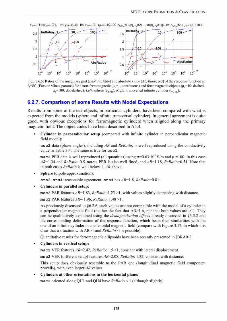
MD FEATURE EXTRACTION & CLASSIFICATION
6.2.7. Comparison of some Results with Model ExpectationsResults from some of the test objects, in particular cylinders, have been compared with what isexpected from the models (sphere and infinite transversal cylinder). In general agreement is quitegood, with obvious exceptions for ferromagnetic cylinders when aligned along the primarymagnetic field. The object codes have been described in A5.4.
• Cylinder in perpendicular setup (compared with infinite cylinder in perpendicular magneticfield model):coc2 data (phase angles), including AR and ReRatio, is well reproduced using the conductivityvalue in Table 3.4. The same is true for coc1.msc2 PER data is well reproduced (all quantities) using σ=0.63·107 S/m and µr=100. In this caseAR=1.34 and ReRatio~0.5. msc1 PER is also well fitted, and AR=1.18, ReRatio=0.51. Note thatin both cases ReRatio is well below 1, AR above.
• Sphere (dipole approximation):sts2, sts4: reasonable agreement. sts4 has AR=1.8, ReRatio=0.81.
• Cylinders in parallel setup:msc2 PAR features AR=1.83, ReRatio: 1.23 >1, with values slightly decreasing with distance.msc1 PAR features AR= 1.96, ReRatio: 1.48 >1.As previously discussed in §6.2.6, such values are not compatible with the model of a cylinder ina perpendicular magnetic field (neither the fact that AR>1.6, nor that both values are >1). Theycan be qualitatively explained using the demagnetization effects already discussed in §3.5.2 andthe corresponding deformation of the response function, which bears then similarities with theone of an infinite cylinder in a solenoidal magnetic field (compare with Figure 3.17, in which it isclear that a situation with AR>1 and ReRatio>1 is possible).Quantitative results for ferromagnetic ellipsoids have been recently presented in [BRA01].
• Cylinders in vertical setup:msc2 VER features AR=2.42, ReRatio: 1.5 >1, constant with lateral displacement.msc2 VER (different setup) features AR=2.08, ReRatio: 1.32, constant with distance.This setup does obviously resemble to the PAR one (longitudinal magnetic field componentprevails), with even larger AR values.
• Cylinders at other orientations in the horizontal plane:msc2 oriented along QU1 and QU4 have ReRatio < 1 (although slightly).
Figure 6.5: Ratios of the imaginary part (ImRatio, blue) and absolute value (AbsRatio, red) of the response function at f2=8f1 (Förster Minex params) for a non-ferromagnetic (µr=1, continuous) and ferromagnetic objects (µr=10: dashed,
µr=100: dot-dashed). Left: sphere (χSPH), Right: transversal infinite cylinder (qCYL).
100 101 102 103 104 105 106 107Α
0.5
1
1.5
2
2.5
ΧSPH�f1����ΧSPH�f2��, �Im�ΧSPH�f1����Im�ΧSPH�f2�� �Μr�1,10,100
ImRatioc, 1 10 100
1
10 100
AbsRatioc
100 101 102 103 104 105 106 107Α
0.5
1
1.5
2
2.5
�qCYL�f1����qCYL�f2��, �Im�qCYL�f1����Im�qCYL�f2�� �Μr�1,10,100�
ImRatioc, 1 10 100
1
10 100
AbsRatioc
173

CHAPTER 6
6.3. Classification Opportunities
In the following we will analyse the distribution of the previously defined features and discuss theresulting object classification opportunities, that is the possibility of attributing a measurement toa specific object class.
The actual values of some features are obviously dependent on the parameters used for theirextraction, such as the minimum distance between peaks in the phase angle histograms or thevarious thresholds; they are also specific of the Förster Minex operating parameters. The resultsshould nevertheless still be of general interest and it should not be too difficult to extrapolatethem to other operating conditions.
“Small” vs. “Large” ObjectsThe features we are looking at are basically derived from the target’s response function and assuch do depend on its response parameter75 (or induction number), as discussed in §3.1 and §3.3.The latter is usually a product of permeability, conductivity and the square of an average lineardimension of the target, thereby putting a particular weight on its size.
In the following we will therefore often refer to an object size using terms such as “small” and“large”; strictly speaking we are however discriminating on the full response parameter ratherthan on its physical size only.
6.3.1. Phase Angle Peaks and Amplitude Ratio DistributionWe analyse the distribution of the phase angle peaks and of the (average) amplitude ratio ARusing 3D scatter plots, each phase angle peak ϕj being represented as a point in 3D space with thefollowing cylindrical coordinates (θ,ρ,z):
• θ =ϕj and ρ=1; • z=AR. If there are two or more peaks for a given entry all of them are associated to the same value
of AR.
In addition we plot for each point its projection on the x-y plane and connect it with a line to theorigin76, to make it easier to determine each point’s phase. Examples are shown in Figure 6.6, the
75. And on its orientation (influence of the demagnetization factor) for most ferromagnetic objects.
Figure 6.6: Phase angle peaks (left: all, right: highest average amplitude only) vs. average amplitude ratio for deb01-14&16 (blue circles: values at f1, red squares: values at f2). Attention, scale(x)=1/2scale(y).
76. Actually on a plane at z = –0.5, for graphical reasons only.
0
0.2
0.4
0.6
0.8
1
−1
−0.5
0
0.5
1−0.5
0
0.5
1
1.5
2
2.5
3
Re(f1), Re(f2); normIm(f1), Im(f2); norm
Am
plitu
de r
atio
debris−list01−16: All peaks
0
0.2
0.4
0.6
0.8
1
−1
−0.5
0
0.5
1−0.5
0
0.5
1
1.5
2
2.5
3
Re(f1), Re(f2); normIm(f1), Im(f2); norm
Am
plitu
de r
atio
debris−list01−16: Highest average amplitude peaks
174

MD FEATURE EXTRACTION & CLASSIFICATION
left plot containing all phase angle peaks, the right one only the highest average amplitude peaks.Points at f1 are shown with blue dots, at f2 with red squares. Note that the scale along x is 1/2 ofthe scale along y. The corresponding AR distribution is shown in Figure 6.8 (AR>1 for allferromagnetic objects, AR<1 for the two non-ferromagnetic ones).
The resulting distributions of the phase angle peaks only, i.e. the projections on the x-y plane,confirm in a quantitative way the qualitative results detailed in the previous chapter.
In addition the complete distributions (i.e. considering AR as well) detail how different objectcategories, in particular debris, can form clusters in the chosen 3D space. Examples are shown inFigure 6.7, the non-ferromagnetic foils deb20-26 in the top left corner (very low AR), theferromagnetic foils deb30-37&39 in the top right corner (AR~1), and all ferromagnetic debris(1<AR<2.2 with a couple of exceptions) in the bottom half. Note in particular the trend, in thislast case, of decreasing phase angle with increasing amplitude ratio.
Figure 6.7: Phase angle peaks (highest average amplitude only) vs. average amplitude ratio for deb20-26 (non-ferromag. foils, background subtracted), deb30-37&39 (ferromag. foils), and all ferromag. debris.
0
0.2
0.4
0.6
0.8
1
−1
−0.5
0
0.5
1−0.5
0
0.5
1
1.5
2
2.5
3
Re(f1), Re(f2); normIm(f1), Im(f2); norm
Am
plitu
de r
atio
debris−list20−26BGND: Highest average amplitude peaks
0
0.2
0.4
0.6
0.8
1
−1
−0.5
0
0.5
1−0.5
0
0.5
1
1.5
2
2.5
3
Re(f1), Re(f2); normIm(f1), Im(f2); norm
Am
plitu
de r
atio
debris−list30−37−39: Highest average amplitude peaks
00.2
0.40.6
0.81
−1
−0.5
0
0.5
1−0.5
0
0.5
1
1.5
2
2.5
3
Re(f1), Re(f2); normIm(f1), Im(f2); norm
Am
plitu
de r
atio
debris−list−Ferro: Highest average amplitude peaks
175
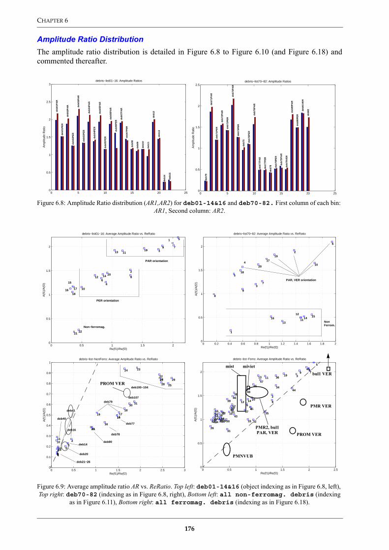
CHAPTER 6
Amplitude Ratio DistributionThe amplitude ratio distribution is detailed in Figure 6.8 to Figure 6.10 (and Figure 6.18) andcommented thereafter.
Figure 6.8: Amplitude Ratio distribution (AR1,AR2) for deb01-14&16 and deb70-82. First column of each bin: AR1, Second column: AR2.
Figure 6.9: Average amplitude ratio AR vs. ReRatio. Top left: deb01-14&16 (object indexing as in Figure 6.8, left), Top right: deb70-82 (indexing as in Figure 6.8, right), Bottom left: all non-ferromag. debris (indexing
as in Figure 6.11), Bottom right: all ferromag. debris (indexing as in Figure 6.18).
0 5 10 15 20 250
0.5
1
1.5
2
2.5
3
Am
plitu
de R
atio
debris−list01−16: Amplitude Ratios
deb
01P
AR
deb
01P
ER
deb
02P
AR
deb
02P
ER
deb
03P
AR
deb
03P
ER
deb
04P
AR
deb
04P
ER
deb
05P
AR
deb
05P
ER
deb
06P
AR
deb
06P
ER
deb
07P
AR
deb
07P
ER
deb
08
deb
09
deb
10
deb
11
deb
12
deb
13
deb
14
deb
16
0 5 10 15 20 250
0.5
1
1.5
2
2.5
Am
plitu
de R
atio
debris−list70−82: Amplitude Ratios
deb
70
deb
71P
AR
deb
71P
ER
deb
72P
AR
deb
72P
ER
deb
73P
AR
deb
73P
ER
deb
75 deb
76P
ER
deb
76P
AR
deb
77P
AR
deb
77P
ER
deb
78 deb
79P
ER
deb
79P
AR
deb
79V
ER
deb
80P
AR
deb
80P
ER
deb
81V
ER
deb
82
0 0.5 1 1.5 20
0.5
1
1.5
2
debris−list01−16: Average Amplitude Ratio vs. ReRatio
Re(f1)/Re(f2)
A(f
1)/A
(f2)
1
2
3
4
5
6
7
8
9
10
11
12
13
14
15
16 17
18
19
20
2122
PAR orientation
PER orientation
Non−ferromag.
0 0.2 0.4 0.6 0.8 1 1.2 1.4 1.6 1.8 20
0.5
1
1.5
2
debris−list70−82: Average Amplitude Ratio vs. ReRatio
Re(f1)/Re(f2)
A(f
1)/A
(f2)
1
2
3
4
5
6
7
8
9
10
11
12
13
14 1516
17
18
19
20
NonFerrom.
PAR, VER orientation
0 0.5 1 1.5 2 2.5 30
0.1
0.2
0.3
0.4
0.5
0.6
0.7
0.8
0.9
1debris−list−NonFerro: Average Amplitude Ratio vs. ReRatio
Re(f1)/Re(f2)
A(f
1)/A
(f2)
12
3
456789
1011
1213
1415
16
1718
19
2021
22
2324
25
2627
2829
3031
deb100−104
deb107
deb77
deb79
deb78
deb16
deb14
deb20
deb40
deb21−26
deb90
deb41
0 0.5 1 1.5 2 2.50
0.5
1
1.5
2
debris−list−Ferro: Average Amplitude Ratio vs. ReRatio
Re(f1)/Re(f2)
A(f
1)/A
(f2)
1
2
3
4
5
6
7
8
9
10
11
12
13
14
151617
18
19
20
2122 2324 25
26
27282930
31
3233
34
35
36
37
38
39
40
41
42
43
4445
46
47
48
495051
52
5354
5556
PMNVUB
PROM VER
PMR VER
bul1 VER
mist miviet
PMR2, bul1 PAR, VER
PROM VER
176

MD FEATURE EXTRACTION & CLASSIFICATION
Its main characteristics are:• AR>1 typical of ferromagnetic objects with few exceptions, usually due to very weak or irregular
signals.• AR~1-1.2 for flat ferromagnetic objects;• AR>1.5 typical of elongated ferromagnetic objects when there is a significant component of the
magnetic field along the symmetry axis (e.g. PAR, VER orientations).In general: AR(PAR, VER orientations) > AR(PER orientation) for a given elongated object,and similarly for ReRatio.
• AR<0.2-0.3 typical of small non-ferromagnetic objects (e.g. foils);• 0.7<AR<1 typical of large non-ferromagnetic objects (e.g. deb100-104, Figure 6.9) or large
ferromagnetic ones (e.g. PROM, Figure 6.10).These results are in general in good agreement with model expectations. Note that a maximumvalue of about 1.9 is foreseen for a sphere and of 1.6 for a transversal (infinite) cylinder using theFörster Minex operating parameters (see the corresponding plots in Figure 6.5).
Stainless steel cylinders with a small residual permeability represent special cases (see thediscussion in §6.2.6).
Figure 6.10: Amplitude Ratio distribution (AR1,AR2) and Average amplitude ratio AR vs. ReRatio. First row: low metal content mines and their components, Second row: PMN and large metallic mines/UXO.
0 2 4 6 8 10 12 14 16 18 200
0.5
1
1.5
2
2.5
3
Am
plitu
de R
atio
mines−list1−small: Amplitude Ratios
mli1
1b.0
14 (
mid
erea
l)
mid
ePA
R
mid
ePE
R
mid
eVE
R
mid
eVE
R−1
00
mli1
1f.0
14 (
mis
trea
l)
mis
t−01
0
mis
t−03
0
mis
t−05
0
mis
t1P
ER
mis
t1P
AR
mis
t1V
ER
mli1
1c.0
13 (
mic
h@
5cm
)
mli1
1c.0
14 (
mic
h@
5cm
)
mli1
1c.0
15 (
mic
h@
5cm
)
mli1
1g.0
14 (
mic
h@
10cm
)
miv
iet
miv
iet−
100
0 0.1 0.2 0.3 0.4 0.5 0.6 0.7 0.8 0.9 10
0.2
0.4
0.6
0.8
1
1.2
1.4
1.6
1.8
2mines−list1−small: Average Amplitude Ratio vs. ReRatio
Re(f1)/Re(f2)
A(f
1)/A
(f2)
123 45
6
78
9
10
11 12
131415
16
17 18
midereal
mist
miviet
mide
mich
0 5 10 15 20 25 30 350
0.5
1
1.5
2
2.5
3
3.5
4
Am
plitu
de R
atio
mines−list1−large: Amplitude Ratios
pm
nV
UB
PA
R1
pm
nV
UB
PA
R2
pm
nV
UB
PE
R1
pm
nV
UB
PE
R2
pm
nV
UB
PA
R1
pm
nV
UB
PA
R2
pm
nV
UB
PE
R1
pm
nV
UB
PE
R2
pm
nV
UB
PA
R1−
050
pm
nV
UB
PA
R1−
100
pm
nV
UB
PA
R1−
200
pm
nV
UB
PA
R1−
260
pro
mV
ER
pro
mV
ER
pro
mV
ER
pm
r2V
ER
pm
r2V
ER
pm
r2V
ER
pm
r2P
AR
1
pm
r2P
AR
2
pm
r2P
ER
1
pm
r2P
ER
2
bu
l1V
ER
do
wn
bu
l1V
ER
up
bu
l1V
ER
do
wn
bu
l1V
ER
up
bu
l1P
AR
1
bu
l1P
AR
2
bu
l1P
ER
1
bu
l1P
ER
2
bu
l1P
AR
1−10
0
bu
l1P
AR
2−10
0
bu
l1P
ER
1−10
0
bu
l1P
ER
2−10
0
0 0.5 1 1.5 20
0.5
1
1.5
2
2.5
3
3.5mines−list1−large: Average Amplitude Ratio vs. ReRatio
Re(f1)/Re(f2)
A(f
1)/A
(f2)
123456789101112
131415
16 1718
19
2021
22
23
24
25
26
2728
29 3031
3233 34
bul1VER down@025mm
up@025mm
down@100mm
up@100mm
PMR2VER
PROM VER
PMR2 PAR,PER
bul1 PAR,PER
PMNVUB
177

CHAPTER 6
6.3.2. Amplitude Ratio and Real Part Ratio DistributionExamples of the average amplitude ratio AR vs. ReRatio distribution are shown in Figure 6.9 andFigure 6.10. It is evident that the two features are correlated: the higher AR, the higher ReRatio,with some exception for very large ferromagnetic objects. This corresponds to a trend from smallobjects in the lower left corner (all non-ferromagnetic debris plot) to large ones in the upper rightcorner, i.e. when moving from the resistive to the inductive limit.
This implies that for non-ferromagnetic objects one can extrapolate to a certain extent the sizefrom the AR vs. ReRatio plot, which is generally not true for ferromagnetic objects without somea priori knowledge of target type and/or orientation.
In the case of the debris most non-ferromagnetic objects are below the AR=ReRatio line (dashedline in the bottom plots of Figure 6.9), as correctly predicted by the sphere and cylinder model,whereas all ferromagnetic debris is above it. The models also foresee a maximum ReRatio ofabout 2.8, which is experimentally well verified.
It is interesting to note that some very large ferromagnetic objects could be distinguished on thebasis of their (AR,ReRatio) values alone, for example a vertical PMR-2A or bul1.
In general however only a partial target discrimination seems possible using the (AR,ReRatio)values alone, as evident from the bottom plots in Figure 6.9, on which the distribution of severalclasses of targets of interest – extracted from Figure 6.10 – has been superposed. The residualambiguity can be resolved in a number of cases using the phase response information.
ReRatio DistributionThe ReRatio distribution by itself presents the following characteristics:
• ReRatio<0.2-0.3 typical of small non-ferromagnetic objects such as foils or wire strands. This ismostly true also for similar ferromagnetic objects;
• ReRatio>2.0-2.5 typical of large non-ferromagnetic objects.• In general: ReRatio(PAR, VER orientations) > ReRatio(PER orientation) for a given
elongated ferromagnetic object, similarly to the AR behaviour.ReRatio works therefore well to discriminate very large or very small non-ferromagnetic objects.It does however not seem to be sufficiently robust, used by itself, for ferromagnetic objects (toomuch influence of permeability and demagnetization factor). Some targets could be discriminatedon the basis of their ReRatio alone, such as the small mine components, however likely at theprice of a high false alarm ratio.
6.3.3. L/R (Simple Circuit Model)Results for all non-ferromagnetic debris are shown in Figure 6.11. In most cases there is goodagreement between L/R|f1, L/R|f2 and L/R|∆Weighted. Errors are apparent for weak signals such as inthe case of deb21-26 and deb40-41, but in these cases there is room for improvement.
The resulting values are also well correlated with object “size” (comparing with thecorresponding position in the bottom left plot of Figure 6.9) and phase angle behaviour (notshown). The values for the mide and midereal mine detonators (not shown) are in the range0.13-0.19 and are also in good agreement amongst themselves; as a comparison, they are of thesame order as the first three debris items in Figure 6.11.
As expected L/R does deliver inconsistent results for ferromagnetic or composite objects.
178

MD FEATURE EXTRACTION & CLASSIFICATION
6.3.4. Delta ZSeveral phase response distributions of the differential signal DeltaZ as defined in §6.2.5 areshown in Figure 6.12, having considered only the phase angle peaks with the highest averageamplitude. Note that usually positive phase angles result when ReRatio>1, negative ones whenReRatio<1.
As already hinted at, results depend heavily on the individual signal amplitudes and are as aconsequence definitely more variable than other features. From the experimental data it appearsin particular that two or more quite different objects can produce a similar DeltaZ phase angle,which can therefore in general not be inverted.
Some object categories do however partially cluster. For example, the DeltaZ phase angle of mostfoils, whether ferromagnetic or not, is close to the horizontal (0°), probably due to their smallReRatio value (see deb21-26 and deb30-36 in Figure 6.12, an exception being the large foilconstituting deb20). Also, a sizeable fraction of small to medium ferromagnetic objects – of theorder of 50% – have a DeltaZ phase close to the vertical (say in the window +90° to +70° or –90°to –70°, see again Figure 6.12).
DeltaZ could therefore still useful to eliminate foils and some small ferromagnetic pieces –obviously provided the targets have a different behaviour, which was true in the cases we lookedat – even in presence of background signal fluctuations.
As an alternative approach we note that the phase of DeltaZ for the small mide mine detonator,which does also contain a foil, seems to be quite stable with orientation/distance at around –52° to–60° (–68° for midereal), a feature which could be exploited if necessary by discardingobjects with different characteristics, together with its ReRatio for example. The small minestriker pin (mist) does also behave in a similar way. The robustness of such an approach vis-à-vis other mine components has obviously to be checked in detail.
Figure 6.11: L/R (simple circuit model) at f1, at f2 and using a weighted difference (see text), for all non-ferromag. debris
5 10 15 20 25 30
0
0.5
1
1.5
2
debris−list−NonF: L/R at f1, f2 and for DeltaWeighted
deb
14 deb
16
deb
20
deb
21
deb
22
deb
23
deb
24
deb
25
deb
26d
eb40
PA
R deb
40P
ER
deb
41P
AR
deb
41P
ER
deb
77P
AR
deb
77P
ER
deb
78
deb
79P
ER
deb
79P
AR
deb
79V
ER
deb
90P
AR
deb
90P
ER
deb
100
deb
101P
AR
deb
101P
ER
deb
102
deb
103P
AR
deb
103P
ER
deb
104P
AR
deb
104P
ER
deb
107P
AR
deb
107P
ER
L/R, f1L/R, f2L/R, DeltaWeighted
179

CHAPTER 6
Summarising and simplifying, DeltaZ could be used, probably at the price of a higher false alarmrate, when the S/N ratio is too weak and the other features fail, either to discard some objects (e.g.foils) or provided we know what we are looking for.
6.3.5. Ferromagnetic FlagA “ferromagnetic flag” could be raised when either AR>1 (or say AR>0.9 with some tolerance),ϕ1>0 or ϕ2>0. This works well for all cases except for very large ferromagnetic objects such asthe PROM mine (§5.9.1). It does not necessarily mean that the whole objects is ferromagnetic,only that it contains a ferromagnetic component.
Figure 6.12: DeltaZ Phase angle peaks (highest average amplitude only). Top left: deb01-14&16, Top right: deb20-26 (non-ferromag. foils, background subtracted), Bottom left: deb30-37&39 (ferromag. foils), Bottom
right: low metal content mines and their components.
−0.5 0 0.5 1 1.5
−1
−0.8
−0.6
−0.4
−0.2
0
0.2
0.4
0.6
0.8
1
Re(DeltaZ); norm
Im(D
elta
Z);
nor
mdebris−list01−16: DeltaZ: Highest average amplitude peaks
1
2
3
4
5
6
78 9
10
11
12
13
14
1516
1718
19
20
2122
−0.5 0 0.5 1 1.5
−1
−0.8
−0.6
−0.4
−0.2
0
0.2
0.4
0.6
0.8
1
Re(DeltaZ); norm
Im(D
elta
Z);
nor
m
debris−list20−26BGND: DeltaZ: Highest average amplitude peaks
1
2 3
4 567
−0.5 0 0.5 1 1.5
−1
−0.8
−0.6
−0.4
−0.2
0
0.2
0.4
0.6
0.8
1
Re(DeltaZ); norm
Im(D
elta
Z);
nor
m
mines−list1−small: DeltaZ: Highest average amplitude peaks
1
23
45
6 789101112 13
14
15161718
−0.5 0 0.5 1 1.5
−1
−0.8
−0.6
−0.4
−0.2
0
0.2
0.4
0.6
0.8
1
Re(DeltaZ); norm
Im(D
elta
Z);
nor
m
debris−list30−37−39: DeltaZ: Highest average amplitude peaks
1
23
4
5
678
9
180

MD FEATURE EXTRACTION & CLASSIFICATION
6.4. Conclusions
Whereas the previous chapter focused more on the qualitative aspects of the phase responsebehaviour, in this chapter we have defined a number of features, processed the available data andanalysed the resulting feature distributions.
6.4.1. Overall ConsiderationsThe peak finding algorithm in particular seems to be working well; this allows to reduce thedetailed curves in the complex plane to a coarser information, basically the phase angle peaks andtheir average amplitudes. Multiple peaks are usually characteristic of composite or ferromagneticobjects, or for low S/N scenarios. One large ferromagnetic peak is usually strongly indicative of aferromagnetic component.
Most of the information seems to be contained in the phase response. There are however cases inwhich the use of the amplitude ratio AR, and of the ReRatio, provides additional information, inparticular helping in resolving ambiguities. Examples are the response of a large ferromagneticitem such as the PROM mine, or of stainless steel objects with a small residual permeability. Ingeneral only a partial target discrimination seems possible using the (AR,ReRatio) values alone(see §6.3.2 for details).
The models’ predictions on the behaviour of AR and ReRatio are confirmed by the experimentaldata, similarly to the phase response which we already discussed in the previous chapter.Important demagnetization effects are apparent for elongated ferromagnetic objects, for whichAR(PAR, VER orientations) > AR(PER orientation), and similarly for ReRatio.
6.4.2. Main ConclusionsWe conclude by A) first commenting on the possibility of a coarse object classification based onthe object size and permeability (ferromagnetic or not), B) moving then to the possibility ofdiscriminating large objects (metallic mines, UXO), and finally C) mines in general.
A) Coarse Object Classification PossibleA coarse target classification according to the object size, as defined at the beginning of §6.3, andpermeability (ferromagnetic or not), seems indeed to be possible, at least for scenarios with asufficient S/N ratio.
The decision could be taken by the user himself relying on a visual interface of the typediscussed in the last chapter (complex plane curves), or using a simplified bidimensionalinformation like the phase angle peaks, possibly augmented by an indication of the amplituderatio if necessary. A simple alternative could be represented by a plot in the AR vs. ReRatio plane.This type of scenario could apply to a hand-held system, where the user analyses each alarm, andshould in any case be very useful for development purposes.
An alternative is represented by an automated system with a direct output indicating the mostlikely object size and permeability (ferromagnetic or not). A possible outline of the resultingsimplified user interface is sketched in A6.4. This could be combined if necessary with a 2Ddiagram of the phase response.
Whether these type of approaches are sufficient for actual mine discrimination is discussed inmore detail at C).
In the low S/N case detection is still possible but classification gets increasingly difficult (forquantitative considerations on this topic using time domain signals see also [GEN99, TAN01]).Apart from deciding not to attempt classifying a signal with insufficient S/N, when the main
181

CHAPTER 6
features can not be used reliably any more it should still be possible to exploit features such asReRatio, L/R|∆Weighted and DeltaZ albeit with reduced discrimination capabilities.
B) Large Metallic Mines/UXO DiscriminationWe recall that our initial idea was to discriminate large targets relying on their phase response, forexample by imposing a threshold on the phase. The results for some large metallic objects (PROM,PMR, bul1) confirm that this is possible, at least for the object we looked at. Composite objectsdo definitely deserve a closer look.
It can however be necessary to complement the phase response with AR to resolve ambiguities,such as in the case of a PROM.
We initially hoped to extend this discrimination approach also to mines with an average metalliccontent (e.g. PMN, PMN2). Judging from the experimental results this might be possible for thePMN if the signature from the ring is reasonably stable. It looks more difficult for the PMN2,which is composed of about 10 pieces (Figure 5.4) of various sizes. This mine delivers a mostlyferromagnetic response, but not equivalent to that of a single larger target; it might however stillbe possible to distinguish it from non-ferromagnetic and from smaller ferromagnetic items.
C) Mine DiscriminationDiscriminating mines from clutter or even different mines among themselves looks feasible; inthe end it depends however on the following factors:
• Which and how many types of mines are present (a priori knowledge).Examples: if we are looking for minimum-metal mines containing a detonator similar to themide previously analysed, we could in principle discard all ferromagnetic objects. Similarly, ifthe target is an object similar to the small nail representing the mist mine striker pin one couldpossibly exclude a number of non-ferromagnetic debris items.Too many different types are likely to make a purely visual choice quite difficult.
• How much one can rely on stable mine signatures. This influences the tolerance “windows”which will have to be applied around the known targets of interest.We can distinguish two aspects here: differences at the mine component level, and differences inthe behaviour of a given type of object.The first point has already been discussed in some detail in §5.12. It includes manufacturingdifferences as well as the use of different components altogether (see also §5.8.3). Along the samelines [DRU00b] discusses differences in the response of a “new” and an “old” PMN mine due torusting of the cover retaining ring. It is also well known that water can infiltrate into some mineswith time, and if ferromagnetic components are present they are likely to rust as well. Similarly,in the case of previous mechanical clearance the mine can be broken and its pieces separated, witha corresponding change in signature. This takes us back to possible a priori knowledge.The second point relates mostly to changes in the response of ferromagnetic or composite objectsfor different orientations/distances. They affect the phase response, as discussed in detail in thelast chapter, as well as other features as analysed in this chapter.
Note that the fact of having to look at too many different objects and/or of having to use too largewindows will probably affect the selectivity of the procedure and the resulting false alarm rate.
• How representative the debris we had available is, and how often multitarget scenarios areencountered.
• How many clutter objects have a sufficient S/N ratio to allow discrimination.Indeed, even provided that one can discriminate mines from clutter, the actual systemeffectiveness will depend on how much the false alarm rate can be reduced, i.e. how many timesa clutter item has a sufficient S/N to be identified as such. In other words, clutter is usually vastlymajoritary; therefore, even if we could identify each mine but for example only 10% of the clutter
182

MD FEATURE EXTRACTION & CLASSIFICATION
had a sufficient S/N (i.e. in nearly 90% of the cases we would have to issue an “unknown objecttype” response), the system would probably not be too useful.An object’s S/N ratio is influenced in particular by its depth and size. Additionally the soil typedoes obviously play a crucial role. We will comment in the following on the depth distributionwhen looking for mines (UXO might be different, as the typical target depths are larger).It has been reported that most debris is close to the surface, which would be beneficial, but we arenot aware of large scale quantitative studies in this direction apart from [JOY02]77. Anecdotalevidence exist on the use by some deminers of small permanent magnets to remove small nearsurface ferromagnetic items; along the same lines tests have been carried out with large magnetsmounted on the rear of vehicles, for example during the vegetation cutting phase, which can onlywork if most debris is close to the surface.In order to have some preciser quantitative indications we have gone back to the original resultsof the Cambodia data collection campaign [GUE97] from which most of the debris we analysedhas been derived. All approximate depth indications have been summarised in Table 6.1, for atotal of 64 objects; when the depth was within a range of values we have taken the largest one. The distribution of this limited sample is concentrated in the upper 10 cm, with nearly 3/4 of alltargets in the first 5 cm.
From the original notes one can also calculate that 26 objects were clearly ferromagnetic, 12clearly non-ferromagnetic, and the remaining 26 of a priori unknown nature. In 3 cases themetallic debris causing the metal detector alarm was too small to be found.
In situations where one can not rely on stable signatures it could still be possible to excludecertain types of clutter (e.g. foils); it remains however to be seen how useful this is.
6.4.3. Additional Considerations on Object DetectionConcerning the Förster Minex detector specifically, it does not seem to be easy, when looking atthe detection of metallic object (no classification attempts), to do better than what alreadyimplemented without compromising on the robustness side. This might also depend on the factthat we operate on digital signals, i.e. after the A/D conversion, instead of working on the originalanalogic signals.
There are however a few cases where an amelioration of the detection efficiency might bepossible in the case of non-conductive soils78, relying on the real parts of the received signals aswell as on DeltaImag. An example of target objects for which such an approach could be usefulare the stainless steel cylinders we analysed, which are probably paramagnetic and whoseimaginary part of the received signal is small.
77. During the VAMIDS metal detector array test detailed in §1.3, every piece the hand-held detectors signalled wasweighted and inspected, and “most of the false signals were pieces of shrapnel and metal junk like wire and bottletops that were either on top or in the first 10mm of soil.” [JOY02].
Depth (cm) 0 1 2 3 4 5 6 7 8 9 10 10+
# of objects 4 9 10 6 6 12 1 3 4 – 7 2
Table 6.1: Example of debris depth distribution (extracted from [GUE97]; d=0: “on the surface”)
78. When the real part of the received signal is mostly background unaffected.
183
CHAPTER 6
Bibliography
[BRA01] H. Braunisch, C. O. Ao, K. O’Neill, and J. A. Kong, “Magnetoquasistatic Response ofConducting and Permeable Prolate Spheroid Under Axial Excitation”, IEEE Transactions onGeoscience and Remote Sensing, v. 39, no.12, pp. 2689-2701, Dec. 2001
[DRU00b]P. Druyts, Y. Yvinec, and L. Merlat, “Signal processing tools for standard metal detectors(Imaging and Signature mode)”, in Proc. of the Research on Demining Technologies JointWorkshop, Joint Research Centre (JRC), Ispra, Italy, 12-14 July 2000.
[FRI01] M. Fritzsche, “Anwendung von Verfahren der Mustererkennung zur Detektion von Landminenmit Georadaren”, Forschungsberichte aus dem Institut für Höchstfrequenztechnik undElektronik der Universität Karlsruhe (TH), Band 30, W. Wiesbeck Ed., Karlsruhe University(Germany), June 2001 (in German). ISSN: 0942-2935.
[GUE97] F. Guerne, description of the DeTeC2 GPR Cambodia data taking, EPFL/DeTeC Website.Available from http://diwww.epfl.ch/lami/detec/
[GEN99] N. Geng, C. E. Baum, and L. Carin, “On the Low-Frequency Natural Response of Conductingand Permeable Targets”, IEEE Trans. on Geoscience and Remote Sensing, vol. 37, no. 1, pp.347-359, Jan. 1999.
[JOY02] Joynt, V. “National Mine Action: Problems and Predictions”, Journal of Mine Action, MineAction Information Center at the James Madison University, Issue 6.1, 2002, pp. 37-41.Available from http://maic.jmu.edu/journal/6.1/index.htm
[LOC02] J. Lochy, “Acquisition and Analysis of Metal Detector Data for Humanitarian DeminingApplications”, VUB-ETRO-IRIS “Werkkollege” Internal Report, April 2002.
[PAT99] W. Patzwaldt, “Method for the operation and for the evaluation of signals from an eddy currentprobe and device for performing the method“, US Patent #6,005,392, 21 Dec. 1999.
[SAR97] B. I. Saracik, “Improvements in Metal Detection Technology”, The University of WesternAustralia, Dept. of Mechanical and Materials Engineering (supervisor Prof. J. Trevelyan), B.Eng. Thesis, October 1997, 103 pp.
[SIG02] Sigrist, C., and Bruschini, C., “Metal Detectors for Humanitarian Demining: a Patent Searchand Analysis”, EUDEM2 report, May 2002. Available from http://www.eudem.vub.ac.be/
[SZY98] P. Szyngiera, and A. Wojtasik, “Wavelet Transformation Applied for Eddy-Current MetalDetector Signals Analysis”, in Proc. of the Conference of Telecommunication, Bydgoszcz,Poland, 1998 (Proceedings in Polish).
[TAN01] S. L. Tantum, and L. M. Collins, “A Comparison of Algorithms for Subsurface TargetDetection and Identification Using Time-Domain Electromagnetic Induction Data”, IEEETrans. on Geoscience and Remote Sensing, vol. 39, no. 6, pp. 1299-1306, June 2001.
[WAV01]M. Misiti, G. Oppenheim, J.-M. Poggi, and Y. Misiti, “MATLAB® Wavelet Toolbox User’sManual”, v. 2.1 (Release 12.1), July 2001.
184

MD FEATURE EXTRACTION & CLASSIFICATION
Appendix A6.
A6.1. FilteringA number of tests have been carried out to reduce the background influence in the imaginarycomponent of the received signal. “Standard” techniques to deal with this aspect in the case offrequency domain systems do often consist in some form of bandpass or highpass filtering,relying on the fact that the target signal does usually change over a much shorter distance than thebackground (i.e. that background fluctuations are “slow” – see also §2.3.3.2 and the patentsreferenced in [SIG02]). The very low frequency signal components are therefore associated withthe background signal fluctuations.
In the case of the signals we looked at the spectral position of the signal did actually represent aproblem, as the low frequency signal components and the background fluctuations did often fallinto the same spectral region. This is also due to the fact that the signals are already differential innature, the background having already been reduced to first order.
“Classical” Filtering TechniquesSeveral techniques were tried with partial success in specific cases, but no single robust techniquecould be identified. Using “classical” filtering techniques the best results were obtained with:
• A highpass filter with a very low frequency pole (e.g. a Chebyshev Type I Infinite ImpulseResponse minimum order filter);
• The first or second derivative of the signal;• A lowpass filter with a very large window, 200 samples wide say (corresponding to about 10 cm),
to obtain an approximation of the signals’ low frequency components. This approximation canthen be subtracted from the input quantities;
• The elimination of a linear trend.Some of the previously mentioned filters, such as taking the derivative, do generate significantsignal distortions. This should however not represent a problem when the aim is to calculate thesignal’s phase and the filter is applied to both the real and imaginary component79.
“Adaptive” FiltersPartial success was also obtained using the real components as a template for the imaginary ones.The basic idea is that in a number of cases the phase response is quite constant, which means thatthe real and imaginary component as a function of position, at a given frequency, have the sameshape. As the real component is mostly unaffected in non-conductive soils, it can be used astemplate. DeltaImag could be used as well in a number of situations.
Deconvolution was carried out isolating the relevant portion of the real component at eachfrequency and using it as deconvolution “kernel” (or Point Spread Function, PSF) of a Wienerfilter. The results seem however to be quite dependent on the right choice of the PSF and thenoise level present in the data.
79. The use of linear phase filters has been recommended by some authors.
185
CHAPTER 6
Wavelet Based FilteringWavelet transforms have seen an increased use in the past 15 years in signal analysis applied to anumber of different domains. We shall provide in the following a brief introduction to the subject,without pretending to be exhaustive; most material has been extracted from [WAV01], which alsocontains a list of the main references to the subject, and to a lesser extent from [FRI01].
A wavelet is a waveform of effectively limited duration – i.e. of compact support – that has anaverage value of zero, and wavelet analysis is a linear technique which can be described as thebreaking up of a signal into shifted and scaled versions of the original (or mother) wavelet.Wavelet analysis can therefore be described as a windowing technique with variable-sizedregions and uses a time-scale region (scale can be connected in a broad sense to frequency).
This has to be compared to Fourier analysis, which consists of breaking up a signal into sinewaves of various frequencies and whose main drawback is that transforming to the frequencydomain time information is lost80, or with the Short-Time Fourier Transform (STFT) for example,which maps a signal into a two-dimensional function of time and frequency, using the Fouriertransform to analyse only a small section of the signal at a time (using the same window at allfrequencies). The STFT does therefore represent a sort of compromise between the time- andfrequency-based views of a signal: it provides some information about both when and at whatfrequencies a signal event occurs.
The Continuous Wavelet Transform (CWT) is defined as the sum over all time of the signal f(t)multiplied by scaled (i.e. stretched or compressed), shifted (i.e. delayed or anticipated) versionsψa,b(t) of a mother wavelet function ψ(t):
(6.14)
The results are the wavelet coefficients C(scale,position)=C(a,b), a>0, which are function of thescale a and position b, and of the shape of the chosen wavelet obviously:
(6.15)
The wavelet coefficients basically represent how closely correlated the scaled and shifted waveletis with the signal under analysis (actually a section of it, given that the wavelet has a limitedduration), like for a correlation coefficient. The corresponding plots, in which the x axisrepresents position along the signal (time), the y axis represents scale and the colour at each xypoint represents the magnitude of the wavelet coefficient C, are the time-scale view of the signalwe referred to earlier. Examples are provided in Figure 6.13.
The higher the scale a, the more “stretched” the wavelet, the longer the portion of the signal withwhich it is being compared, and thus the coarser (slowly changing) the signal features beingmeasured by the wavelet coefficients (high scale → low frequency).
Unlike the discrete wavelet transform described below, the CWT can operate at every scale; it isalso continuous in terms of shifting: during computation, the analysing wavelet is shiftedsmoothly over the full domain of the analyzed function.
80. When looking at a Fourier transform of a signal, it is impossible to tell when a particular event took place.
ψscale position, t( ) ψa b, t( ) 1a
-------ψ t b–a--------
= =
C scale position,( ) C a b,( ) f t( ) 1a
-------ψ t b–a----------
td∞–
∞
∫= =
186

MD FEATURE EXTRACTION & CLASSIFICATION
The Discrete Wavelet Transform (DWT) shares the same basic ideas using a only a subset ofscales and positions, in particular “dyadic” scales and positions (i.e. based on powers of two) forwhich efficient implementation schemes exist with just as accurate results as the CWT.
Without entering into too many details of the DWT implementation, let us mention that inwavelet analysis one often speaks of approximations A and details D. The approximations arethe high-scale, low-frequency components of the signal, the details are the low-scale, high-frequency components. An input signal might be decomposed in its A and D components, of samelength as the input signal, with an appropriate pair of complementary lowpass/highpass filters.
What happens in practice is that the input signal is downsampled after filtering producing twosequences, cA containing the DWT approximation coefficients and cD containing the DWT detailcoefficients, each being about half as long as the input signal. The decomposition process canthen be iterated with a cascade of filters (a filter bank), with successive approximationcoefficients being decomposed in turn, so that one signal is broken down into many lowerresolution components.
This multiple level decomposition is called the wavelet decomposition tree and results, at a givenlevel N, in one sequence cAN containing the DWT approximation coefficients at level N, and Nsequences cD1-cDN containing the DWT details coefficients:
Wavelet decomposition tree result (at level N): S → cAN ; cD1, cD2, ..., cDN (6.16)
The value of N is selected in practice on the basis of the nature of the signal, or on a suitablecriterion such as the entropy. The length of the coefficient sequences is decreasing at each levelby about a factor of two (at least for the first levels).
In a similar way the DWT coefficients can be used in an inverse process, the Inverse DiscreteWavelet Transform (IDWT), to reconstruct the original signal without loss of information usingappropriate lowpass/highpass reconstruction filters (and signal upsampling), which are notnecessarily equal to the decomposition filters81. The choice of the filters determines whetherperfect reconstruction is possible; in general the wavelet coefficients are modified beforereconstruction.
It is in particular also possible to reconstruct the approximations Ai and details Di themselves,which have the same length as the original signal, from their coefficient vectors82. In addition itcan be shown that there are actually several ways of reassembling the original signal S:
(6.17)
To construct a wavelet of some practical utility, it usually makes more sense to design theappropriate quadrature mirror filters, and then use them to create the waveform, instead ofstarting by drawing the waveform first hand. This approach implies that the choice of the filtersdetermines the shape of the wavelet used to perform the analysis, and in general we can notchoose an arbitrary wavelet waveform if we want to be able to reconstruct the original signalaccurately.
81. The decomposition filters, together with their associated reconstruction filters, form a system called quadraturemirror filters.
82. For example at the first level, the coefficient vectors cA1 and cD1 have been produced by downsampling and areonly half the length of the original signal; they cannot directly be combined to reproduce the signal. It isnecessary to reconstruct the approximations and details before combining them.
S A1 D1+ A2 D2 D1+ + A3 D3 D2 D1+ + + … AN Dii 1=
N
∑+= = = = =
187

CHAPTER 6
The wavelet function ψ in particular is determined by the highpass filter, which also produces thedetails of the wavelet decomposition. There is an additional scaling function φ associated withsome, but not all wavelets; it very similar to the wavelet function and is determined by thelowpass quadrature mirror filters, and thus associated with the approximations of the waveletdecomposition.
Finally, it has to be noted that the DWT is not a time-invariant (translation invariant) transform.
Denoising is one of the classical applications of wavelet analysis and represents an alternative totechniques such as lowpass filtering.
Wavelet based denoising is efficient, at least in its basic implementation, for families of functionsthat have only a few non zero wavelet coefficients, i.e. having a sparse wavelet representation,such as a function which is smooth almost everywhere83 [WAV01]. It basically consists incarrying out a wavelet decomposition at a given level N, and applying for each level a thresholdto the details coefficients. Several threshold selection rules exist, as well as the possibility ofapplying local (time-dependent) thresholds.
The filtered signal is then calculated with an inverse transform using the original approximationcoefficients of level N and the modified details coefficients of levels 1 to N. Note that such a“traditional” wavelet based de-noising on channels affected by drift (low frequency trends) doesnot eliminate the drift itself.
An example of an application to metal detector laboratory data is provided in [SZY98]. We havealso carried out tests using wavelet based denoising, however without apparent improvement withrespect to standard lowpass filtering.
Additional tests were therefore carried out with a different aim, namely signal detrending, i.e.reducing the mostly low frequency component present in the imaginary part of the signal due tobackground (soil) fluctuations. The basic idea is to exploit the fact that wavelets ψ can be foundwhose first M+1 moments are vanishing:
(6.18)
If the analysed signal S is a polynomial of degree M, then the coefficients C(a,b) = 0 for all a andall b. In other words, such wavelets automatically suppress the polynomials. The degree of S canvary with time, provided that it remains less than M. If S is a polynomial of degree M on segment[α,β], then C(a,b) = 0 as long as the support of the function is included in[α,β]. The suppression is local and effects appear on the edges of the segment.
As a consequence the details are also zero. In practice this means that the details obtained with awavelet of sufficiently high order should not be sensitive to constant, linear, quadratic etc.components. We have tried to exploit this property together with the fact that we have in firstapproximation reference channels, f1REAL and f2REAL (and possibly DeltaImag), whichindicate where the signal is concentrated and which form it has. Overall this seems only partlysuccessful.
83. Thinking of the original signal to be retrieved, i.e. not yet affected by noise.
tpψ t( ) td( ) td∞–
∞
∫ 0 for 0 p M≤ ≤=
1 a⁄( )ψ t b–( ) a⁄( )
188

MD FEATURE EXTRACTION & CLASSIFICATION
Continuous Wavelet Transform (CWT) ResultsContinuous analysis is often easier to interpret, since its redundancy tends to reinforce the traitsand makes all information more visible. Thus, the analysis gains in “readability” and in ease ofinterpretation what it loses in terms of saving space [WAV01].
We will therefore first show selected examples using the Continuous Wavelets Transform, toillustrate data processing improvement possibilities. We have concentrated on Gaussianderivative wavelets , which have a form similar to the signal we are looking for; thisshould lead to a reduced number of coefficients with significant amplitude (i.e. a maximum ofinformation is concentrated in a reduced number of coefficients [FRI01]). Log Gabor waveletshave been preferred in [SAR97], where the aim was to retrieve the depth information.
Gaussian derivative wavelets (gausN) are derivatives of the Gaussian probability densityfunction (Eq. (6.19)), where CN is such that the 2-norm of is 1. gausN has N vanishingmoments.
(6.19)
We have chosen to work using scale values a of 1 to 128 in increments of 2. For each given scalea the wavelet coefficients C(a,b) are computed for a position b = 1 to ls=length(S). The resultsabout to be shown do therefore correspond to a coefficient matrix C(1:2:128, ls). Two types ofscenarios have been investigated:
• Enhancing the detection of weak signals not affected by background fluctuations (f1REAL,f2REAL and DeltaImag):Results using gaus1 are shown in Figure 6.13 in the form of copies of the Matlab WaveletToolbox graphical user interface images. The topmost section of each plot shows the signal beinganalysed (already lowpass filtered, scale in mV), the second the absolute value of the CWTcoefficients (coloured by scale), the third one line of coefficients at a given intermediate scale(a=63), the fourth a plot of local maxima of coefficients across scales.The peaks correspond to the position of the centre of the signal (i.e. the zero crossing) and allowto find and reshape it. They could also be used to find the coefficients of interest for the filteringof f1IMAG, f2IMAG.The first plot features f1REAL in a “high” S/N case; the clear peak at position 500 across allscales corresponds to the signal’s zero crossing.The bottom plots feature f1REAL and f2REAL respectively in a low S/N case (weak signals). Thecoefficient’s structure is still clearly visible and similar to the previous case, the peak around 500-520 corresponding to the signal’s zero crossing.
• Filtering signals affected by background fluctuations (f1IMAG, f2IMAG):Results using gaus2 are shown in Figure 6.14: the peaks correspond now to the position of thesignal’s peaks (i.e. maximum and minimum) and should allow to remove linear trends (#vanishing moments(gaus2)–1=1). To remove higher order trends it would be necessary to moveto gaus3, etc., or to other higher order wavelets. The left plot features f1IMAG in a low S/N case. The coefficient’s structure is however stillclearly visible, with peaks at 400-420 and 590 (compare with Figure 6.13, top), and does notshow the trend of original signal any more. In this case gaus1 could also work. Qualitativelysimilar results are obtained using db2 (Daubechies wavelet of order 2).The right plot features f2IMAG in the same setup, with an even poorer S/N; the weak originalsignal is very strongly background affected. In this case gaus1 would not work well. Thecoefficients do not show the trend of original signal any more, are however quite weak in the areaof interest.
ψ N( ) t( )
ψ N( ) t( )
ψ N( ) t( ) CNxN
N
dd e x2–=
189

CHAPTER 6
Discrete Wavelet Transform (DWT) ResultsSelected examples using the Discrete Wavelet Transform (DWT) are shown in Figure 6.15. Inthis case we have used compactly supported biorthogonal spline wavelets (bior of order Nr.Nd,where r stands for reconstruction and d for decomposition84), in particular bior3.3 and to alesser extent bior3.1. In the second case the reconstruction wavelet is quite similar to aGaussian, in the first it is similar to the derivative of a Gaussian. The number of vanishingmoments for the decomposition wavelet is Nr–1.
Figure 6.13: Continuous Wavelet Transform (CWT) results using gaus1 for mist flush (mine w/o detonator). Top: f1REAL, detector@80mm; Bottom left: f1REAL, det.@160mm; Bottom right: f2REAL, det.@160mm.
84. In this case two wavelets are indeed used, one for decomposition and another for reconstruction.
190

MD FEATURE EXTRACTION & CLASSIFICATION
We have again investigated the possibility of filtering signals affected by backgroundfluctuations, partly relying on the insensitivity of the details to low order polynomials when usingwavelets with a sufficient number of vanishing moments.
We define a Reference signal, f1REAL or f2REAL, and a Target signal, f1IMAG or f2IMAGrespectively, and decompose them via DWT up to a level N, which results in two sets ofapproximation coefficients cAN and details coefficients cD1 to cDN. We then choose, for one ofthe two signals (usually the Reference, but we also tried to inverse the roles in S3,S4), the firstmaxRetainedCoeff coefficients with the highest absolute values according to a strategy definedbelow, and retain the same coefficients of the other signal; all other coefficients are zeroed. Theresulting IDWT reconstructed signals are then plotted.
The following coefficient selection strategies S1 to S4 have been trialled, with results displayedin Figure 6.15 for maxRetainedCoeff = 5, 7 and 10, Reference=f1REAL and Target= f1IMAG(original signals dashed):
• S1: Consider ALL coefficients (cAN, cD1-cDN), and base the choice of those to retain on theReference signal.This is a simplified form of the “traditional” wavelet based de-noising schemes.The basic idea is to use the “clean” channel (no background fluctuations) as Reference, identifyits most important coefficients and use the corresponding ones of the Target for its reconstruction.The hope is that the coefficients which contain the “drift” contribution in the Targetdecomposition will not be selected.Two examples are shown in the top row of Figure 6.15: the Reference is well fitted, whereas wetend to select “only” the portion of the initial Target signal which is in correspondence with thesignificant parts of the reference signal; this is only moderately useful.
• S2: Consider the DETAILS coefficients only (cD1-cDN), and base the choice on the Referencesignal (its approximation coefficients cAN are explicitly zeroed; the Target approximationcoefficients are therefore automatically zeroed as well).As we are not considering the approximation it is necessary to use the higher levels (starting from8-9 say) to get some meaningful results; examples are shown in the middle row of Figure 6.15.The background fluctuation are indeed attenuated, other fluctuations are however introduced; it isnot straightforward to assess their importance.
Figure 6.14: Continuous Wavelet Transform (CWT) results using gaus2 for mist flush (mine without detonator). Left: f1IMAG, detector@80mm; Right: f2IMAG, detector.@80mm.
191

CHAPTER 6
• S3: Consider ALL coefficients (cAN, cD1-cDN), but base the choice on the Target signal directly.Examples are shown in the bottom row of Figure 6.15. If we take a sufficiently highdecomposition level (ex. 8, 9) and number of coefficients (~10), we basically retain theapproximation coefficients and the reconstructed signal approximates the drift. At a lower level(ex. 5, 6) the details definitely play a marginal role, we are basically selecting only the largestapproximation coefficients. This type of strategy does therefore not seem to work.
• S4: Consider the DETAILS coefficients only (cD1-cDN), and base the choice on the Target signaldirectly (its approximation coefficients cAN are explicitly zeroed; the Reference approximationcoefficients are therefore automatically zeroed as well).Results are similar to those of S2. The reconstruction seems however to work best for the filewhose coefficients are used for the choice (in this case the Target file, for S2 the Reference file).
Overall S1 and S2 seem to work best, but tuning of the coefficient selection and choice of theappropriate decomposition level are not straightforward and need to be guided by a preciserquantitative analysis.
[SZY98] does use a DWT version without decimation (downsampling), also called DiscreteStationary Wavelet Transform, for metal detector data instead of the standard DWT, whichaccording to the authors would introduce phase angle distortions. The aim is denoising rather thandetrending (no significant background fluctuations are visible in the data), the argument mighthowever still be valid.
192

MD FEATURE EXTRACTION & CLASSIFICATION
Figure 6.15: Discrete Wavelet Transform (DWT) results using bior3.3 for different coefficient selection strategies S1-S3 and decomposition levels N. Top: S1, left: N=7, right: N=8; Middle: S2, left: N=8, right: N=10; Bottom: S3,
left: N=8, right: N=6. In all cases: Ch1=f1REAL, Ch2= f1IMAG, original signal dashed.
0 200 400 600 800 1000 1200 1400−0.4
−0.2
0
0.2
0.4
0.6mich−080−ch1: DWT reconstructed signal − bior3.3 up to Level 7
ampl
itude
(m
V)
5 710
0 200 400 600 800 1000 1200 1400−4
−3
−2
−1
0
1
2
3mich−080−ch2: DWT reconstructed signal − bior3.3 up to Level 7
samples
ampl
itude
(m
V)
5 710
0 200 400 600 800 1000 1200 1400−0.06
−0.04
−0.02
0
0.02
0.04
0.06mich−162−ch1: DWT reconstructed signal − bior3.3 up to Level 8
ampl
itude
(m
V)
5 710
0 200 400 600 800 1000 1200 1400−0.6
−0.4
−0.2
0
0.2
0.4mich−162−ch2: DWT reconstructed signal − bior3.3 up to Level 8
samples
ampl
itude
(m
V)
5 710
0 200 400 600 800 1000 1200 1400−0.4
−0.2
0
0.2
0.4
0.6mich−080−ch1: DWT reconstructed signal − bior3.3 up to Level 10
ampl
itude
(m
V)
5 710
0 200 400 600 800 1000 1200 1400−4
−3
−2
−1
0
1
2
3mich−080−ch2: DWT reconstructed signal − bior3.3 up to Level 10
samples
ampl
itude
(m
V)
5 710
0 200 400 600 800 1000 1200 1400−0.4
−0.2
0
0.2
0.4
0.6mich−080−ch1: DWT reconstructed signal − bior3.3 up to Level 8
ampl
itude
(m
V)
5 710
0 200 400 600 800 1000 1200 1400−4
−3
−2
−1
0
1
2
3mich−080−ch2: DWT reconstructed signal − bior3.3 up to Level 8
samples
ampl
itude
(m
V)
5 710
0 200 400 600 800 1000 1200 1400−4
−2
0
2
4mide−000−025−1−ver−test7.6−ch1: DWT reconstructed signal − bior3.3 up to Level 8
ampl
itude
(m
V)
5 710
0 200 400 600 800 1000 1200 1400−1.5
−1
−0.5
0
0.5
1mide−000−025−1−ver−test7.6−ch2: DWT reconstructed signal − bior3.3 up to Level 8
samples
ampl
itude
(m
V)
5 710
0 200 400 600 800 1000 1200 1400−4
−2
0
2
4mide−000−025−1−ver−test7.6−ch1: DWT reconstructed signal − bior3.3 up to Level 6
ampl
itude
(m
V)
5 710
0 200 400 600 800 1000 1200 1400−1.5
−1
−0.5
0
0.5
1mide−000−025−1−ver−test7.6−ch2: DWT reconstructed signal − bior3.3 up to Level 6
samples
ampl
itude
(m
V)
5 710
mist flush (mine w/o detonator), det.@80mm S3, Level8 mide VER flush (mine detonator), det.@25mm S3, Level6
mide VER flush (mine detonator), det.@25mm S2, Level8 mist flush (mine w/o detonator), det.@80mm S2, Level10
mist flush (mine w/o detonator), det.@80mm S1, Level7 mist flush (mine w/o detonator), det.@160mm S1, Level8
193

CHAPTER 6
A6.2. Feature Definition and Extraction – Additional Examples
Phase Response
Figure 6.16: Phase response calculation and phase angle peak representation for a minimum-metal mine detonator replica (mide; example of small non-ferromagnetic object), vertical, flush.
−2 0 2
−8
−6
−4
−2
0
2
4
6
8
Re(f1) vs Im(f1) over RoI1
mV
mV
−10 0 10
−30
−20
−10
0
10
20
30
Re(f2) vs Im(f2) over RoI2
mV−5 0 5
−20
−15
−10
−5
0
5
10
15
20
DelRe vs DelIm (all, f2−f1)
mV
−100 −80 −60 −40 −20 0 20 40 60 800
20
40
60
80
100
120Histogram for phase of frequency 1
Phase angle
# of
poi
nts
−70 −60 −50 −40 −30 −20 −10 0 10 20 300
50
100
150
200
250
300Histogram for phase of frequency 2
Phase angle
# of
poi
nts
−100 −80 −60 −40 −20 0 20 40 60 80 1000
100
200
300
400Histogram for phase of DeltaZ (freq. difference)
Phase angle
# of
poi
nts
1
2
3
30
210
60
240
90
270
120
300
150
330
180 0
Phase angle peaks for f1Area: proportional to relative peak frequency
Length: average amplitude in mVLegend: Phase / Peak Frequency / Average Amplitude
−8.87 0.2 2.71 −44 0.021 0.919
5
10
15
30
210
60
240
90
270
120
300
150
330
180 0
Phase angle peaks for f2Area: proportional to relative peak frequency
Length: average amplitude in mVLegend: Phase / Peak Frequency / Average Amplitude
−48.5 0.44 12.3
5
10
30
210
60
240
90
270
120
300
150
330
180 0
Phase angle peaks for DeltaZ (frequency differencing)Area: proportional to relative peak frequency
Length: average amplitude in mVLegend: Phase / Peak Frequency / Average Amplitude
−56.7 0.28 9.35
194

MD FEATURE EXTRACTION & CLASSIFICATION
Figure 6.17: Phase response calculation and phase angle peak representation for a real (live) minimum-metal mine (mich; example of composite object), flush with detector at 5 cm. [mli11g]
−0.4 −0.2 0 0.2 0.4
−1
−0.5
0
0.5
1
Re(f1) vs Im(f1) over RoI1
mV
mV
−1 0 1
−3
−2
−1
0
1
2
3
Re(f2) vs Im(f2) over RoI2
mV−0.5 0 0.5
−1.5
−1
−0.5
0
0.5
1
1.5
DelRe vs DelIm (all, f2−f1)
mV
−40 −20 0 20 40 60 80 1000
50
100
150
200Histogram for phase of frequency 1
Phase angle
# of
poi
nts
−100 −80 −60 −40 −20 0 20 40 60 800
50
100
150
200
250Histogram for phase of frequency 2
Phase angle
# of
poi
nts
0.5
1
30
210
60
240
90
270
120
300
150
330
180 0
Phase angle peaks for f1Area: proportional to relative peak frequency
Length: average amplitude in mVLegend: Phase / Peak Frequency / Average Amplitude
54.6 0.34 0.628
0.5
1
1.5
30
210
60
240
90
270
120
300
150
330
180 0
Phase angle peaks for f2Area: proportional to relative peak frequency
Length: average amplitude in mVLegend: Phase / Peak Frequency / Average Amplitude
−38.2 0.32 1.25−52.4 0.058 0.33
−100 −80 −60 −40 −20 0 20 40 60 80 1000
50
100
150
200Histogram for phase of DeltaZ (freq. difference)
Phase angle
# of
poi
nts
0.5
1
1.5
30
210
60
240
90
270
120
300
150
330
180 0
Phase angle peaks for DeltaZ (frequency differencing)Area: proportional to relative peak frequency
Length: average amplitude in mVLegend: Phase / Peak Frequency / Average Amplitude
−68 0.2 1.22−52.8 0.11 0.118−37.6 0.034 0.0594
195

CHAPTER 6
A6.3. Classification Opportunities – Additional Examples
Amplitude Ratio Distribution
Figure 6.18: Amplitude Ratio distribution (AR1,AR2) for all ferromagnetic debris. First column of each bin: AR1, Second column: AR2.
0 10 20 30 40 50 600
0.5
1
1.5
2
2.5
Am
plitu
de R
atio
debris−list−Ferro: Amplitude Ratios
deb
01P
AR
deb
01P
ER
deb
02P
AR
deb
02P
ER
deb
03P
AR
deb
03P
ER
deb
04P
AR
deb
04P
ER
deb
05P
AR
deb
05P
ER
deb
06P
AR
deb
06P
ER
deb
07P
AR
deb
07P
ER
deb
08d
eb09
deb
10d
eb11
deb
12d
eb13
deb
30 deb
31d
eb32
deb
33d
eb34
deb
35d
eb36
deb
37d
eb39
deb
50P
AR
deb
50P
ER
deb
51P
AR
deb
51P
ER
deb
52P
AR
deb
52P
ER
deb
71P
AR
deb
71P
ER
deb
72P
AR
deb
72P
ER
deb
73P
AR
deb
73P
ER
deb
75 deb
76P
ER
deb
76P
AR
deb
80P
AR
deb
80P
ER
deb
81V
ER
deb
82d
eb92
deb
93d
eb94 d
eb95
deb
105P
AR
deb
105P
ER
deb
106P
AR
deb
106P
ER
196

MD FEATURE EXTRACTION & CLASSIFICATION
A6.4. Example of Simplified User Interface & Object Size ClassificationScheme
Figure 6.19 reproduces the possible outline of the simplified user interface mentioned in §6.4.2,where the individual object sizes correspond to the coarse target classification discussed therein.We have added two categories, UNKNOWN corresponding to targets with either too weak S/N ratioor not fitting any category (e.g. situations with some composite object, or very irregularresponses, or multitarget scenarios), and DANGER, triggered when the target resembles either alarge object in the case of UXO, or one of a given set of mines (or mine components).
This interface could be combined if necessary with a 2D diagram of the phase response, eithercontinuous or already with phase angle peaks and average amplitudes, at least during thedevelopment phase.
An object could well be associated to different (neighbouring) sizes, or perhaps to allferromagnetic sizes if it clear that its nature is ferromagnetic but it is impossible to say more.
A possible object size classification scheme based on three parameters, the phase angle responseat f1 and f2, ϕ1 and ϕ2 respectively, and the amplitude ratio AR, is proposed in Table 6.2. It ismostly based on the observation of the response of the debris items, taking certain categories asrepresentative of a size, for example (NF: non-ferromagnetic, F: ferromagnetic):
• Very small: NF: deb21-26 (foils), F: deb30-39 (foils);• Small: NF: deb20 (foil), deb40-41, F: deb01-07 (PER), deb92-95 (fragments);• Medium: NF: deb90 (spent cartridge), F: deb80-82 (shell fragments);• Large: NF: deb100-104, F: PMR (stake mine).
The phase angle ranges are indicated as (upper limit):(lower limit), which is somewhat naturalgiven that the phase angles normally decrease with increasing object size. The lower AR end forferromagnetic objects for the first classes has been taken as 0.9 instead of 1 to cope with somemeasurement uncertainties.
Figure 6.19: Classification opportunities: possible outline of simplified user interface with coarse object size/type classification
Object Size, Non-Ferromagnetic Object Size, Ferromagnetic
Feature VerySmall Small Medium Large Very
Small Small Medium Large
AR <0.2 0.2:0.5 0.3:0.7 0.7:1 0.9:1.1 0.9:1.5 >1.5 0.5:1.5?
ϕ10:–5 –10:–20 –20:–60 <–60 90:85 85:75 75:55 55:0
ϕ20:–10 –10:–50 –50:–70 <–70 90:80 80:60 60:45 <ϕ1
Table 6.2: Possible object classification scheme. All phase angles are in degrees; the phase angle ranges are indicated as (upper limit):(lower limit), the opposite for AR.
FERROMAGNETIC NON-FERROMAGNETIC
VERYSMALL
SMALL MEDIUM LARGEVERY
SMALLSMALL MEDIUM LARGE
UNKNOWN DANGER
? !
197

CHAPTER 6
The choice of the different classes is obviously somewhat fuzzy, and is complicated by theorientation dependence of the response for a number of ferromagnetic targets, in particular theelongated ones (demagnetization effects). Other features could be included as well, such asmultiple phase angle peaks; we have implicitly relied on one phase angle peak per frequency, theone with largest average amplitude. The phase angle ranges have been taken here as non-overlapping, different choices are again possible, and probably required in order to cope withspecial cases such as very large ferromagnetic objects (e.g. PROM metallic mine).
198

7. Metal Detector Near Field Imaging
An approach which is complementary to the one described in the previous chapterconsists in providing information on the object’s size and shape, which could beuseful in discriminating in certain circumstances mines and/or UXO from clutter.“Conventional” metal detectors can indeed be used to generate images of buriedmetallic objects with varying levels of resolution.
After a brief look at the electromagnetic near field properties we will review anumber of existing systems and approaches, to concentrate then on two portablehigh resolution applications which exploit the geometrical properties of the nearfield. The first features a commercial multisensor system designed for NdTapplications in civil engineering, the second concentrates on the application of imagedeblurring techniques (deconvolution) to bidimensional data obtained with acommercially available sensor, the Förster Minex metal detector.
7.1. Low Frequency Electromagnetic Near Field Properties
It is often asked how it is possible, using metal detectors, to detect and/or image objects with aresolution of several (tens of) centimetres when the wavelengths of the applied low frequencyelectromagnetic fields are orders of magnitude larger. The response lies in the fact that the sensorsare operated in the near field – all interactions between the field and scatterers occur in the nearfield of the probe – rather than in the far field as for “classical” imaging applications for example(for which the attainable spatial resolution R is indeed about half of the source wavelength85,R=λ/2 – Rayleigh’s criterion, the resolution is wavelength limited).
The coupling is then by evanescent waves, whose amplitude decreases exponentially along thedirection of propagation, as well as propagating waves in the spectrum of the antennas, andgeometrical properties such as the sensor footprint, scanning pattern and object distance can anddo play a primary role. In the near field the resolution depends on the degree to which theevanescent waves can actually be measured [GUO98 and references contained therein]. As in ourcase the source dimension and the source to detector distance are much smaller than thewavelength in the soil, the ultimate resolution is in fact determined, similarly to what happens forthe imaging of flaws in NdT, by the quasi-static nature of the EM fields that both illuminate thetarget and are scattered by it [BAH88] (see also §3.4.2).
The role that evanescent electromagnetic waves can play is discussed on the basis of a simpleanalytical model in [SMI99] for example. The authors also point to the interesting analogybetween the use of evanescent waves to image a mine and what is done in near field scanningoptical microscopy (NSOM), where evanescent waves are introduced to increase the resolutionbeyond what is possible with a traditional microscope relying only on propagating waves.
It makes therefore sense to measure the induced magnetic field, or its gradient, scanning a singlesensor or using arrays (several combinations of sensing elements are possible), which can bescanned as well, and build a bidimensional image of the measured signal amplitudes86. The latter
85. The attainable resolution R is in general related to the maximum spatial frequency of the field as R=π/kmax.Usually kmax=2π/λ [GUO98].
86. A metal detector does not give directly any depth indication, contrary for example to radar equipment.
199

CHAPTER 7
can then be processed using image processing techniques which rely to variable levels on theknowledge of the underlying physics. In certain cases 3D or pseudo-3D images can bereconstructed as well, or at least some 3D related information recovered (e.g. object depth),exploiting for example multifrequency techniques or the fact that the spatial field behaviour in ahorizontal plane is influenced by the object depth.
7.2. Metal Detector Imaging Systems and Applications
A number of different methodologies and systems have been proposed for the “imaging” ofburied metallic objects of interest to us (mine components, metal mines or UXO), whereby theprecise target application and type of image can be quite different, although emphasis is usuallyon larger targets. Systems range from arrays composed of individual sensors to innovativesensors, sensor geometries and/or processing techniques. Most of them are vehicle based, but afew are designed to be portable.
We will briefly review the most significant ones, as well as holographic techniques in NdT (thedeconvolution approach will be detailed separately in §7.4):
• Scanning Systems:ODIS (Ordnance Detection and Identification System) is a vehicular system using one or moredifferential sensors attached to a rotating arm to scan a path as the sensor platform movesforward. ODIS was conceived to provide the user with quantitative information (relying ondatabase supported inversion) on shallowly buried ordnance and to deliver unprocessed images(not deconvolved) [BOR96, ODIS96]. The latter are very useful to spatially localize the singleobjects, which is essential in a real-time constrained vehicular operation. However, bythemselves, these images probably do not allow because of their resolution to distinguish oneobject from another, except for “large” objects” (i.e. of size comparable to the detector’sdimensions). Additional details are available in the corresponding patents [ESC96,TRI96].
• Metal Detector Arrays:Arrays of metal detectors have also been built, to quickly scan a large path for example, such asthe Schiebel VAMIDS system [RUS99]. Figure 7.1 shows an image corresponding to data takenon a dirt road at DRES [McF96]. Each of the 9 wide strips represents the full width of the array asthe detector moves along the road at uniform speed; the scanning is therefore obtained here by theforward motion of the vehicle alone. Strongly positive signals are white, strongly negative signalsare black. A number of mines are detected, as well as a number of nuisance items and false alarms(courtesy Dr. John McFee, Defence Research Establishment Suffield (DRES), Defence Researchand Development Branch, Canada).
Figure 7.1: Schiebel VAMIDS “image” (McFee, DRES [McF96])
200

MD NEAR FIELD IMAGING
Figure 7.2 (D. Brown, SAIC [BRO96]) shows an image corresponding to data from the scan of aField Calibration lane (low metal clutter) during tests at Ft. A. P. Hill, VA, Nov. 95, using a 2meter array mounted on the multi-sensor VMDT vehicle (Vehicular Mine Detection Testbed)[BRO96]. The large signals are due to metallic mines and the smaller ones to shallowly buriedAPs. It is evident that some form of discrimination based on the size of a spot is possible.
Although VAMIDS was not conceived as an imaging detector, the data it produces can be viewedas low resolution images and existing image processing techniques applied to them. Domain-specific knowledge of metal detector arrays was indeed used and peak detection algorithmssuitably modified, allowing realtime operation. Details are reported in [RUS99], which refers to[DAS90] for the modelling aspects used to analyse the features of the spatial response of the array(replacing the target with an equivalent magnetic dipole induced by the transmit field, and usingthe principle of reciprocity to calculate the voltage induced in a receive coil). This allowed forexample to explain why in a number of instances a white (positive) spot is accompanied by twoblack (negative) spots on each side, as can be seen looking attentively at Figure 7.1.
• Special Coil Configurations (spatial periodicity):Another interesting and unconventional application is represented by the Meandering WindingMagnetometer (MWM) described in [MIT96]. The device, a “planar transformer”, has thecharacteristic of using a square wave winding conductor in order to generate a spatially periodicelectromagnetic field, whose spatial wavelength depends only on the primary winding spatialperiodicity and is the principal reason which allows to model it with accuracy. It can, in principle,detect several characteristics of a buried metallic object (size, shape, etc.) based on a modelledresponse to the spatial wavelength and has spatial imaging capability. Its application tohumanitarian demining has been envisaged, in particular the characterisation of UXO such asunexploded bomblets [GOL98,GOL99].
• Other Sensor Arrays:A portable, low power array of giant magnetoresistive (GMR) sensors has been developed, whichcan also be used for imaging applications [CHA00]. The sensors are arranged in a checkerboardconfiguration (2D array) such that axes of sensitivity of alternate GMR sensors are orthogonallyoriented; other sensor configurations have also been proposed. The preferred target application isUXO remediation via a reduction of the false alarm rate by rapidly distinguishing between buriedordnance and other ferrous items.A similar system featuring a different type of magnetoresistive sensors, of the spin dependenttunnelling type (SDT), is described in [WOL99]. In this case the authors have incorporated thedata analysis algorithms into the design process, with the goal of recovering the target objectparameters – its geometric and material properties – by inverting the measured data usingphysical models of the target (the recovered parameters will then be compared to collections ofmodel parameters for known targets in a database). The theoretical model used to solve thisinverse problem is based on the simplest possible limiting form of the mean field scatteringtheory, which is according to the authors computationally fast and captures the essential physicsin high-contrast scattering; the theory has been specialised for a few canonical shapes.
Figure 7.2: VAMIDS image from VMDT vehicle (D. Brown, SAIC [BRO96])
201

CHAPTER 7
• Holographic Techniques:We have already discussed in §3.4.2 the fact that in the ground the wave equations for the electricand magnetic fields reduce, when displacement currents can be neglected, to diffusion equations.Measurement ranges are usually much less than a wavelength and the corresponding phase delayrelated to the spatial variations of the waves is therefore usually negligible (it is too small to beused to measure an object’s range and shape or to distinguish multiple objects [GUO98]). Themagnitude of the electromagnetic field is however very sensitive, as we know, to the distancefrom the object and to the characteristics of the buried target.Near field electromagnetic “holographic” methods have therefore been devised to achieve animaging resolution not limited by the wavelength resolution limit as in traditional holography87,with the aim of localizing and possibly resolving near-surface buried metallic (i.e. highlyconductive) objects such as UXO and mines [GUO96,GUO98,GUO00].These methods basically rely on the properties of the evanescent waves as already discussed in§7.1. We actually already know that using metal detectors for detection applications it is possibleto achieve a high spatial resolution and are implicitly always working way beyond the wavelengthresolution limit. The interesting point here is the reconstruction of the magnetic field distributionin the horizontal plane at various depths in the ground. This is achieved by propagating themeasured (magnetic) field back to the source plane starting from the measured field above or onthe ground, and relies on the principle that the back-propagated object field will converge at theobject’s true location.In practice this is achieved with a custom designed pulse metal detector, recording the signal atgrid points on a horizontal plane and Fourier transforming it into the frequency domain(amplitude and phase information). The spatial distribution of the magnetic field at a particularfrequency is then Fourier transformed in two dimensions to form a spatial frequency spectrum.This spectrum is multiplied by a propagation function to back-propagate it to a desired depth d,and the result is then inverse Fourier transformed (2D) to produce the reconstructed image at thedepth d.The experimentally achieved resolution was estimated at 10–3 of the wavelength in the conductingmedium (objects located as close as 1 m could be resolved and individually localised with fairlygood accuracy by reconstructing the field images at level planes). It is however not entirely clearhow much the results depend on the electrical ground parameters and their variations(inhomogeneities).
• Holographic Techniques in NdT:Holographic techniques have also been applied in Non-Destructive Testing (NdT) for thereconstruction of volumetric scatterers within conducting materials. In this case one interprets theeddy currents induced in a conductor as penetrating waves, also called “skin waves”, which arestrongly damped due to the skin effect; their wavelength is a factor 2π longer than theirpenetration depth (skin depth). The peculiarity of NdT applications is that due to the presence ofgood conductors the distances involved are much closer to the skin depth – and therefore to thewavelength – than in applications of interest to us; as a consequence phase shifts in the probe fieldcan be exploited.Studies are reported in [HIP90,HIP93] on imaging using broadband holography, in which a coil ismoved along a surface (synthetic aperture like process) whilst scanning a given frequency range.In this case depth resolution is obtained by the use of more than one frequency (single frequencyoperation is detailed for example in [COL84]). A cross-sectional image is generated and its depthresolution increased by phase multiplication of the received multifrequency signals, equivalent toa fictitious reduction of wavelength88. The target application was the imaging of volumescatterers, for example flaws, under a conducting surface. Such volume defects cause localized
87. In traditional holography the hologram is in general recorded several wavelengths away from the source and theevanescent waves play a negligible role.
88. Thus avoiding the need of operating at higher frequencies, which would result in an increase in resolution but atthe price of a smaller skin depth, and therefore of a reduced penetration in the conductor.
202

MD NEAR FIELD IMAGING
conductivity and/or permeability changes in a conductive material, which can be assimilated to aconductive half-space. Typical frequencies are in the range of several tens to hundreds of kHz,with typical spatial dimensions (eddy current probe and associated field) of the order of one mm.The presence of high phase shifts in the probe field does usually favour the application of thistype of technique. These are however the conditions which are usually avoided in the applicationsof interest to us, apart from specific scenarios such as the presence of minimum-metal mines invery conductive soils or close to sea shores for example, working towards higher frequencies(where the skin depth could be of the order of the object depth, see Table 3.2). It is therefore notimmediately clear if such a technique could be transposed with success to demining applications.
Of all the systems discussed, metal detector arrays are probably the most mature ones (see§2.3.2.3 for more details, with description of systems other than VAMIDS). They are in use,mostly as components of multi-sensor vehicle based systems.
The other systems seem to often neglect the soil response, which as we know is correct to firstapproximation only, and which can represent a particular problem when looking at small and/ordeep objects, or in presence of magnetic soil. Their state of maturity is not known with precision.
203

CHAPTER 7
7.3. High Resolution Imaging with a Multisensor Visualising System
We will report in the following on high resolution imaging with a commercial multisensor metaldetector, designed for NdT applications in civil engineering, with the aim of assessing itspotentialities and understanding in a broader sense if such systems, possibly in a modified form,could be useful to tackle some aspects of the humanitarian demining problem along the lines89
proposed in [EBL96]. The latter include the detection of non minimum-metal mines andshallowly buried Unexploded Ordnance (UXO). In fact, given that spatial resolution and depthpenetration constitute conflicting requirements, we do not expect them to be applicable tohumanitarian demining “as is”.
Results could be a priori expected for “larger” metallic objects of regular size which have to bedifferentiated from metallic debris often consisting of small metallic pieces scattered around.Examples are mines with an appreciable metallic content (some grams) such as the Russian PMNor PMN2, or shallowly buried Unexploded Ordnance (UXO) such as “bomblets” which stillplague some areas (e.g. Laos). Minimum-metal mines such as the Chinese Type 72 contain lessthan a gram of metal and seem much less likely to profit from such a system alone, in the sensethat an image of a pointlike object would be of help to the deminer, but in itself probablyinsufficient to take a yes/no decision.
The following sections follow closely [BRU97b,BRU98c,BRU00a].
7.3.1. NdT Applications in Civil EngineeringReinforcing bars are widely employed in civil engineering. They are mostly made of steel,cylindrical, with diameter between 6 mm and 50 mm, and usually located from just underneaththe surface to 18 cm maximum in depth (the shallow location being more frequent).
Rebars in concrete can be detected and characterised using metal detectors, whose task isdefinitely eased by the rebars’ ferromagnetic nature. Simple instruments are only able to locatethe rebars, whereas more advanced ones can also calculate the distance (“cover”) from the surfaceto a rebar of known size and characteristics (this allows to precalibricate the instruments), usuallyoperating by direct contact on a flat surface. Precision on cover measurement can attain somepercent of cover, down to about one mm in the most favourable cases.
The most recent instruments are also able to estimate both cover and rebar size (diameter) bytaking at least two measurements of the same rebar under different conditions. Several techniquesare available [BRU00a].
Different head sizes are sometimes proposed by the manufacturers, and are normally muchsmaller than the ones employed in humanitarian demining. They are therefore more accurate atshallow depths (increased spatial resolution) and able to resolve closely spaced objects, which isespecially useful in “congested” situations, but lack in depth of penetration given that thedetection range is strongly related to the coil dimensions.
Such systems, especially when applied as imaging tools, can indeed exploit the fact that rebarsare shallowly placed regular structures composed of ferromagnetic objects, usually lying in aplane, whereas the humanitarian demining world is obviously much more complex (small andirregular objects, ground inhomogeneities, large number of varying scenarios, etc.). The rejectionof the background signal, for example due to moisture, is therefore also somewhat lessproblematic in civil engineering applications.
89. “First generation equipment [] could provide the deminer with a visual image of shape and size of the metalsignature.”
204

MD NEAR FIELD IMAGING
7.3.2. Imaging Systems for NdT ApplicationsWork on “imaging” devices is indeed in progress, with at least a couple of systems on the market.Note that single sensors have normally to be scanned on the area of interest, which can be timeconsuming; devising a simple and accurate tracking and positioning system is also far fromtrivial. Multi-sensor systems can ease the task at the price of higher cost and somewhat increasedcomplexity; these considerations are valid for humanitarian demining applications as well.Example of developments include the following:
• The University of Kassel has been working on an imaging inductive rebar locator, which uses IRsensors for accurate position measurements (0.5 mm) on a 2D grid of lines [GER96,RIC95].Priority moved then to data analysis and sensor optimization90 more than on imaging aspects(although, concerning the latter, interest in a high resolution tracking system remains).
• The University of Manchester is working on inductive rebar locators and on image processing(enhancement) techniques, such as deconvolution (Figure 7.3 left, c,d) using an accuratelymodelled response function, to sharpen the response. This might require the knowledge of theobject’s depth. Their first generation laboratory prototype used a high resolution positioning frameand a sensor which is physically much smaller than a “conventional” metal detector (Figure 7.3left, a), to improve spatial resolution [GAY94,GAY95]. Recent developments on the sensors aswell as on the signal processing side are detailed in [FER00,GAY00]; the development of a multi-array sensor with a new sensor head has also been pursued.
• The Profomoter4 cover meter developed by Proceq. In addition to the usual functions it is possibleto fit its probe with a path measuring device and, after scanning a surface along the x and ydirection, rebars can be located and displayed on a LCD monitor as shown in Figure 7.3, right.
• The Ferroscan system, developed by the HILTI Corporation, which will be detailed below.We recall that the response curve of a sensor depends on its intrinsic resolution as well as on theobject’s depth, and that it will tend to broaden with increasing depth, which can considerablyaffect the images if left untreated. Figure 7.4 shows examples taken with the Förster Minex.
90. W. Ricken, Private Communication, 9/1997.
Figure 7.3: Left: First generation high resolution imaging metal detector (F. Gaydecki, Manchester [GAY95]). Right: Profometer4 rebar display (example over 50×50 cm).
205

CHAPTER 7
7.3.3. The Ferroscan System91
Ferroscan, manufactured by the HILTI Corporation (Schaan, Liechtenstein), has appeared on themarket at the beginning of the ‘90s and is targeted at the visualization of steel rebars in concrete.
System ComponentsThe heart of the system is represented by the RS 10 multi-sensor scanner (Figure 7.5, right), ofsize 230×140×140 mm and weight 1 kg, which is able to scan a width of 15 cm.
Results are displayed on the RV 10 monitor (Figure 7.5, left), of size 270×200×80 mm and weight2.2 kg (accumulators included). Its backlight LCD works on 320×240 pixels using 9 grey levels.The monitor can be interfaced to a PC via a standard serial RS 232 interface to download theacquired data, with a maximum of 42 raw data files, each one corresponding to a full acquisition(i.e. up to 42 images can be stored). A PC version of the data processing software running on themonitor’s 16 bit microprocessor is also available [HIL94].
Scanning ProcedureThe maximum area which can be covered and analysed in a single image is 60×60 cm and has tobe crossed horizontally and vertically, for a total of eight scans (four in each direction, see Figure7.6).
This because the system, due to its differential nature, is not able to find objects located parallel tothe scanning direction. The latter is in fact strictly true only for rebars somewhat longer than thescan, in the sense that any object shorter than the scan length will produce at least a signal at itsbeginning and at its end; this will have some interesting implications on the objects of interest tous. Note that diagonally lying objects are displayed with slightly worsened resolution (fuzzierimage).
The maximum scanning speed is 0.5 m/s, which looks quite sufficient for hand-held operation; acomplete scan is therefore obtained rather quickly. Note that the area of interest can be smaller ifnecessary, but only sections containing both horizontal and vertical data are actually displayedand analysed [HIL97a].
Figure 7.4: Normalized response at five increasing detector heights starting from 1 cm, innermost: shallow; flush objects. Left: minimum-metal mine, striker pin only (mist), 2 cm increments, Right: msc2, PER orientation, 4 cm
increments (colour code: magenta, cyan, red, green, blue). Horizontal scale in mm.
91. Note: the signature of a Non Disclosure Agreement with the Hilti Corporation was necessary in order to haveaccess to the system’s raw data. As a consequence it is not possible to enter into more detail than what reportedbelow.
300 400 500 600 700 800 900 1000
−1
−0.8
−0.6
−0.4
−0.2
0
0.2
0.4
0.6
0.8
1
mildsteel_cyl2/msc2_010.001 f10+f20 STEP4 filtfilt order 45
300 400 500 600 700 800 900 1000
−1
−0.8
−0.6
−0.4
−0.2
0
0.2
0.4
0.6
0.8
1
minech/mich_010.001 f10+f20 STEP 2 filtfilt order 45, color code mcrgb
206

MD NEAR FIELD IMAGING
The distance is measured along the track by odometry, using an optical encoder, given that thesurface used is almost always flat. One set of two wheels is placed at each end of the scanner, thefour wheels moving together to guarantee displacements as parallel as possible along thescanning direction.
Technical DetailsFrom the Ferroscan patent [KOU94] we know that the system is of multi-sensor and differentialnature, basically measuring (an approximation of) the horizontal gradient, along the scanningdirection, of the vertical component of the induced magnetic field.
Given that such a system is targeted primarily at steel objects it can be built, in principle, eitherusing a permanent magnet or an electromagnet as in conventional metal detectors used forhumanitarian demining, in both cases spanning the scanner width. Corresponding sensors includefield plates such as magnetically controlled resistors, or more conventional copper coils. A twodimensional arrangement of the sensors is in principle possible.
Data ProcessingThe sensor is obviously the central part of the system, but simple and elegant real-time dataprocessing represents an important contribution to system performance too.
Figure 7.5: Ferroscan RV 10 monitor (left) and RS 10 scanner (right) (ruler length: 30 cm)
Figure 7.6: Ferroscan scanning procedure, lengths in cm (from [HIL97a])
207

CHAPTER 7
Using a differential sensor eases rebar localization, which can be obtained for example by lookingfor zero crossings in the received signals, or by further differentiation. The differentiated signalcurves can then be used to produce, starting from the horizontal and vertical scans, a compositebidimensional grey scale image such as Figure 7.7, bottom right [KOU94].
The latter can then be further processed to look at different depth slices, as depicted in the firstthree images of Figure 7.7 (but always starting from 0, e.g. 0 to 20 mm or 0 to 35 mm etc.), usinga simple and efficient menu driven interface and pushbuttons at the side of the screen [HIL97b].Note that these images are binary (black/white). These impressive processing steps rely probablyin a clever way on the characteristics of the rebars’ response, which depends much more on itsdepth than on its size; as such they are not very likely, in their present form, to be generalizedeasily to other metallic objects.
It is well known that the signals received by metal detectors decay very rapidly with distance,spanning several orders of magnitude. Representing with a few grey levels an image of rebars atdifferent depths requires therefore some form of nonlinear transformation to preserve the systemdynamics. This has again implications on the visualization of objects of interest to us, especiallysmall isolated ones. Adequate filtering is also necessary, especially for weak signals.
Note that we did have full access to the system’s raw data thanks to the collaboration of HILTI,but that we did not know the exact details of the algorithm implemented in Ferroscan. We havetherefore tried to reproduce it as simply as possible along the basic lines described above for thepurposes of this study.
Data AnalysisRebars of 6 mm diameter can be displayed nominally down to 130 mm, and those of 36 mmdown to 180 mm. Indication of their depth and size is given only when reliable, which happensfor somewhat smaller values of depth. Sensor resolution is such that two rebars should bedistinguishable when their distance d is greater than their depth (cover) T (d/T≥1).
Note that processing is tuned to ferromagnetic objects; non-ferromagnetic ones, e.g. aluminiumor copper, do also produce signals, which can however not be evaluated. The correspondingimages look somewhat like “negatives” of the expected ones. This does usually not represent aproblem given that the analysis of such objects is not the primary goal of the system, and that theyappear rarely in the context in which Ferroscan is used.
Note also that the magnetic field induced in the bar, or any other (linear) structure, radiates fromits ends in all directions and is often detected in more than one sensor, which contributes tomaking the final image fuzzier [HIL97b]. This effect complements the one described in theScanning Procedure paragraph.
Figure 7.7: Typical Ferroscan B/W rebar images at increasing depth range (0-20 mm, 0-35 mm, 0-50 mm), and overall grey scale image (all depths); 60×60 cm
208

MD NEAR FIELD IMAGING
7.3.4. Ferroscan Results and DiscussionA number of objects were tested during 1997 in a “sandbox” at different depths. For this purposewe put a wooden plate directly on the flattened sand surface and moved the sensor over the platein much the same way as would be done while scanning a standard wall (as described before). Wedo obviously NOT suggest here that this experimental practice is applicable “as is” to thedetection of ordnance or landmines. On the contrary, as for other detectors which have to bescanned in a precise way over the object of interest, an adequate tracking system would have to begiven careful attention and its implementation is far from trivial.
The objects under analysis include (see the corresponding images on the following pages):• Small submunition, steel (ferromagnetic), slight ellipsoidal shape (31×36 mm), 63 grams,
internally prefragmented. • PMN “like” AP mine92 (origin: Cambodia): a “classical” AP mine, diameter 11 cm, height 5 cm,
with cover retaining ring (ferromagnetic!) placed at about 1.5 cm from the top (height 5 mm,thickness about 2 mm, double i.e. bent twice). This mine has usually a steel striker composedessentially of two cylinders joined one to the other, the first of 19 mm length and 9 mm diameter,the second of 39 mm length and 5 mm diameter. This striker is located horizontally somewhatabove the bottom. The one in our possession had in fact a slightly smaller, non-ferromagnetic(alloy?) striker.
• BLU 26 “bomblet” (blue coloured, probably the training version), round (65 mm diameter), 430grams. Its body is likely to be non-ferromagnetic (e.g. aluminium), containing ferromagneticshrapnel. Note that this might be different from the live (all steel?) version93. Large quantities ofsimilar UXO are still found in Laos for example.
• Mortar shell: of total length 300 mm, its top half is steel (ferromagnetic), while the bottom half isaluminium.
• 20mm Projectile: cylindrical, 20 mm diameter at the basis, 140 mm length, steel (ferromagnetic)with an aluminium tip.
• “Rocket”: cylindrical, aluminium, 32-33 cm length.• Debris: a steel screw (ferromagnetic), about 20 mm long, head 7 mm wide, and a large metallic
piece of irregular shape (twisted), 10 mm large and about 3-4 mm thick, probably made of copper(reddish colour).
All of them have been placed flat (horizontally). Further details are available in the next section.
92. It could be a Chinese Type 58 copy (Lyn Haywood, Private Communication).93. Lyn Haywood, Miltra Eng., Private Communication.
209

CHAPTER 7
Figure 7.8: Small submunition (upper left of photograph) (visible ruler length: 13 cm). Top row: original FS images. Bottom row: linear scale. Depth: flush (+1.9cm), 5 cm (+1.9cm), 9 cm (+1.9cm). Image size 30×30 cm
(central section).
210

MD NEAR FIELD IMAGING
Figure 7.9: PMN (see also Figure 5.4). Top row: original FS images. Bottom row: linear scale. Depth from left to right: flush (+1.6cm), 3 cm (+1.6cm). Image size 60×60 cm.
Figure 7.10: BLU26 “bomblet” (lower right of photograph in Figure 7.8). Top row: original FS images. Bottom row: linear scale. Depth: flush (+1.9cm), 3 cm (+1.9cm), 5 cm (+1.9cm). Image size 60×60 cm.
211

CHAPTER 7
Figure 7.11: Mortar shell (ruler length: 30 cm). Top row: original FS images. Bottom row: linear scale. Depth (of the uppermost parts) from left to right: 1-2 cm (+1.6cm), 10-12 cm (+1.6cm). Image size 60×60 cm.
Figure 7.12: 20mm projectile (visible ruler length: 14 cm). Top row: original FS images. Bottom row: linear scale. Depth from left to right: flush (+1.6cm), 6 cm (+1.6cm). Image size 60×60 cm.
212

MD NEAR FIELD IMAGING
Figure 7.13: (UXO) Rocket. Top row: original FS images. Bottom row: linear scale. Depth from left to right: flush (+1.6cm), 8cm (+1.6cm).
Figure 7.14: Debris (large copper, steel screw). Flush (+1.6cm). Left: original Ferroscan image, Right: linear scale. Visible ruler length: 15cm
213
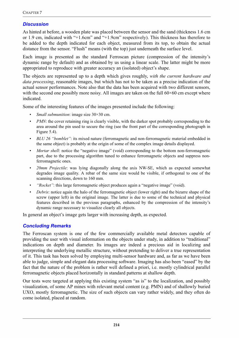
CHAPTER 7
DiscussionAs hinted at before, a wooden plate was placed between the sensor and the sand (thickness 1.6 cmor 1.9 cm, indicated with “+1.6cm” and “+1.9cm” respectively). This thickness has therefore tobe added to the depth indicated for each object, measured from its top, to obtain the actualdistance from the sensor. “Flush” means (with the top) just underneath the surface level.
Each image is presented as the standard Ferroscan picture (compression of the intensity’sdynamic range by default) and as obtained by us using a linear scale. The latter might be moreappropriated to reproduce with greater accuracy an (isolated) object’s shape.
The objects are represented up to a depth which gives roughly, with the current hardware anddata processing, reasonable images, but which has not to be taken as a precise indication of theactual sensor performances. Note also that the data has been acquired with two different sensors,with the second one possibly more noisy. All images are taken on the full 60×60 cm except whereindicated.
Some of the interesting features of the images presented include the following:• Small submunition: image size 30×30 cm.• PMN: the cover retaining ring is clearly visible, with the darker spot probably corresponding to the
area around the pin used to secure the ring (see the front part of the corresponding photograph inFigure 5.4).
• BLU 26 “bomblet”: its mixed nature (ferromagnetic and non-ferromagnetic material embedded inthe same object) is probably at the origin of some of the complex image details displayed.
• Mortar shell: notice the “negative image” (void) corresponding to the bottom non-ferromagneticpart, due to the processing algorithm tuned to enhance ferromagnetic objects and suppress non-ferromagnetic ones.
• 20mm Projectile: was lying diagonally along the axis NW-SE, which as expected somewhatdegrades image quality. A rebar of the same size would be visible, if orthogonal to one of thescanning directions, down to 160 mm.
• “Rocket”: this large ferromagnetic object produces again a “negative image” (void).• Debris: notice again the halo of the ferromagnetic object (lower right) and the bizarre shape of the
screw (upper left) in the original image. The latter is due to some of the technical and physicalfeatures described in the previous paragraphs, enhanced by the compression of the intensity’sdynamic range necessary to visualize clearly all objects.
In general an object’s image gets larger with increasing depth, as expected.
Concluding RemarksThe Ferroscan system is one of the few commercially available metal detectors capable ofproviding the user with visual information on the objects under study, in addition to “traditional”indications on depth and diameter. Its images are indeed a precious aid in localizing andinterpreting the underlying metallic structure, without pretending to deliver a true representationof it. This task has been solved by employing multi-sensor hardware and, as far as we have beenable to judge, simple and elegant data processing software. Imaging has also been “eased” by thefact that the nature of the problem is rather well defined a priori, i.e. mostly cylindrical parallelferromagnetic objects placed horizontally in standard patterns at shallow depth.
Our tests were targeted at applying this existing system “as is” to the localization, and possiblyvisualization, of some AP mines with relevant metal content (e.g. PMN) and of shallowly buriedUXO, mostly ferromagnetic. The size of such objects can vary rather widely, and they often docome isolated, placed at random.
214

MD NEAR FIELD IMAGING
The multi-sensor arrangement is practical to rapidly scan a large area, and its resolution looksindeed sufficiently high for large or extended objects such as UXO and rebars respectively. Onthe other hand using more than one sensor, and the differential arrangement itself, have some sideeffects on the visualization of smaller isolated (ferromagnetic) objects, for which the system wasindeed not intended, and in presence of edges. In these cases a single sensor might be scanned inmore detail over the object, possibly providing a more accurate image.
In any case, the increased spatial resolution comes obviously at the price of decreased depthpenetration, to nobody’s surprise.
Summarizing, the images we have obtained demonstrate that some simple, near real-time highresolution imaging (R=2-3 cm for a flush object) is possible for shallowly buried large orextended targets. Depth penetration improvements seem however necessary for practicalapplications; they could come from the data processing side, for very weak signals for example,and from the sensors, where it has been suggested to use smaller probes, e.g. magnetoresistive orminiature fluxgate elements94 [CZI96] (as discussed for example in §7.2), or to alter the coilgeometry [GAY94] to gain in sensor directivity (“focusing” the magnetic field).
94. Which obviously have to provide the required sensitivity and work at the required frequencies, not at DC asstandard magnetometers.
215

CHAPTER 7
7.4. Shape Determination via Deconvolution
The fact that a raw metal detector “image” is essentially an image of the probe field is well knownin non-destructive testing (NdT) [BAH88]. More accurate imaging results can therefore beexpected by taking into account the detector’s intrinsic response and deconvolving it from themeasured data to obtain an approximation of the object’s real (2D) shape. This work was inspiredby similar R&D in NdT (rebar detection) as already described in §7.3.2 and relies on imageprocessing deblurring techniques.
The simplest approach consists in assuming a linear behaviour, whereby the measured (i.e.degraded) “image” M(x,y) can be written in the spatial domain as a convolution of the real (i.e.original, or true) image R(x,y) and of the detector’s impulse response P(x,y), known in opticalimage processing theory as “Point Spread Function” (PSF), as:
(7.1)
In the image processing domain the PSF represents a distortion operator which describes thedegree to which an optical system blurs (spreads) a point of light [MAT01]. This convolutionprocess is assumed to be correct in most cases in NdT as well [BAH88].
This convolution operation is almost equivalent in the frequency domain to the (element-by-element matrix) multiplication of the corresponding Fourier transforms , that is:
(7.2)
The initial image is therefore obtained by applying in the frequency domain the inverse filter ( , the PSF’s Fourier transform or Optical Transfer Function, describes the
alteration of the image’s spatial frequencies). This is however true only in an idealized scenariowhich does not take into account the presence of noise η(x,y), usually assumed to be additive:
(7.3)
The inverse filter is therefore in practice not always stable due to noise and low values in ,and a stabilized version, the pseudoinverse filter, is often preferred [JAI89]:
(7.4)
As image restoration is basically a high-pass operation it is quite important to avoid noiseamplification. Alternative filtering technique for deconvolution (deblurring) are therefore oftenselected, such as the Wiener filter described for example in detail in [THO98,DRU00].
In our case better results were however obtained using the Lucy-Richardson (LR) maximum-likelihood algorithm, as implemented in an accelerated version in the MATLAB® deconvlucyfunction. The LR algorithm is a member of the family of iterative nonlinear constrained methods.The term nonlinear refers to the fact that, although Eq. (7.1) is still assumed to be valid, thesolution (our estimate of the true image) can not be expressed as a linear function of themeasured image M(x,y). The use of an iterative approach has the advantage of allowing control ofspurious fluctuations by interaction with the solution as it evolves. The notion of “constrained”means that the solution is required to be physically possible (physical-realizability constraints),and implies in practice that bounds are imposed on it. This is frequently synonymous of positivity(amplitude bounds, the solution can not be negative) as in the case of the LR algorithm; spatialbounds are also feasible. Such techniques feature a reduced noise sensitivity with respect totraditional linear methods and have seen an increasing use in the last 20 years or so (for detailssee [JAN97]).
M x y,( ) R x y,( ) P x y,( )⊗=
ℑ
ℑ M( ) ℑ R( ) ℑ P( ) R⇒⋅ ℑ 1– ℑ M( )ℑ P( )--------------
= =
1 ℑ P( )⁄ ℑ P( )
M x y,( ) R x y,( ) P x y,( )⊗ η x y,( )+=
ℑ P( )
Ps 0 when ℑ P( ) ε , Ps< 1 ℑ P( )⁄ otherwise.= =
R x y,( )
216

MD NEAR FIELD IMAGING
The LR algorithm in particular, well known in optics, astronomy, medical imaging, etc., arisesfrom a maximum-likelihood argument in which the image is modelled with Poisson statistics.Multiple iterations are performed maximizing the likelihood that the resulting image, whenconvolved with the PSF, is an instance of the blurred image [HAN97]; the algorithm converges tothe maximum-likelihood solution for Poisson statistics in the data. In practice the result of each iteration is multiplied by a correction factor that relates to the remaining fitting error inthe following way (implying element-by-element division and multiplication as before):
(7.5)
where is the reflected PSF. Note that with a positive initial estimate the successiveestimates will automatically be positive as well. Also, the LR algorithm conserves the totalenergy; it can be effective when the PSF is known, but little information is available about theadditive noise in the corrupted image [MAT01].
In order to avoid overfitting, i.e. fitting statistical fluctuations, it is in fact appropriate to stop theLR iterations before the maximum-likelihood solution is reached. An alternative approach to thesuppression of noise amplification consists in the use of damping techniques. Note that thenumber of iterations necessary to achieve a satisfactory result can depend on the application. Forexample, it has been reported that overfit sets in early when looking at diffuse sources (smoothand extended object), whereas it becomes important only at late iterations for point sources[HAN97]. We have observed a similar behaviour in the metal detector data. Various techniquesfor the algorithm’s acceleration have also been devised.
The Point Spread FunctionThe quality of the deblurred image is in general mainly determined by the knowledge of the PSF.There are basically two approaches to evaluate it: either a set of measurements are taken on small(dipole like) objects, such as spheres, or the detector’s response to such objects is calculated(modelling).
A possible modelling approach consists in calculating the magnetic field generated by thetransmit coil at the target object position; this would allow to calculate the secondary magneticfield, due to the eddy currents, generated by the target object itself. Integration of the latter on thesurface of the receive coil and derivation with respect to time would then lead to the inducedvoltage in the receive coil. An alternative approach consists in replacing the target object withequivalent electric and magnetic dipoles, and then applying the principle of reciprocity to obtainthe voltage induced in the receiver coil [DAS90]. In any case, only in a few cases rigorousanalytical solutions are available (for example for spherical objects and rectangular coils, orcircular coils on their axis). [BAH88] discusses how to compute the PSF for different eddycurrent probe systems, in order to evaluate their imaging characteristics, and points out that ingeneral more than one PSF may be required to characterise a flaw with an eddy current probe, incontrast to optical image processing.
The resulting PSF is in general quite extended compared to the size of typical targets, due to thedetector footprint which is of the order of its diameter. In our case we have chosen to work with aPSF of about 40×40 cm. The image to be deconvolved has also to be large enough to contain thepeak of the target’s response as well as its tails.
As we realised early on [BRU98b], the PSF will actually be a function of the object depth, i.e. bea P(x,y)z (see again Figure 7.4). A somewhat similar situation arises in optical microscopy[SWE97], although in our case the PSF gets broader and flatter with increasing depth and theconcept of in-focus plane does not seem to exist as such. An object’s image will therefore dependon its depth as well, which we can express by rewriting Eq. (7.1) as follows:
Rkˆ x y,( )
Rk 1+ x y,( ) Rk x y,( ) P x– y–,( ) M x y,( )P x y,( ) Rk x y,( )⊗--------------------------------------------⊗
=
P x– y–,( )
217

CHAPTER 7
(7.6)
In optical microscopy ∆z represents a sample’s distance from the in-focus plane, in our case itcould represent the object depth with respect to a fixed reference.
One could actually go one step further and notice that again in optical microscopy it is possible tobuild a three-dimensional image M(x,y,z) of a thick specimen (i.e. of a 3D object) by summingimages from different focal planes, whereby the resulting measured image is the convolution ofthe 3D PSF with the specimen (represented by R(x,y,z) in this case). We could therefore speculatethat a similar procedure is applicable to metal detector data by carrying out scans on differenthorizontal planes, or use coils at different heights.
We will however stick to two dimensional quantities, which already present a sufficient numberof challenges, for example the fact that ferromagnetic objects, in particular elongated ones, arelikely to induce nonlinear features in the acquired images. Whether this approach will bepractically applicable in the field, from the point of view of the resulting resolution, scanningspeed and cost for example, remains therefore to be demonstrated.
7.4.1. 2D Data Taking with a Conventional Metal Detector (Förster Minex)Data was acquired with a Förster Minex metal detector, which as already discussed is of adifferential type. In order to reconstruct a complete map of the horizontal gradient of the verticalcomponent of the induced magnetic field we have therefore decided to add two orthogonalprojections by carrying out two series of parallel scans along the same lines, once with the metaldetector head in the standard position, which we will term A scans, and once with the head in thesame horizontal plane but rotated by 90° (B scans). The use of one projection only, typically the Ascans, might be sufficient in some scenarios.
Each measurement is composed as usual of a magnitude and a phase, or equivalently of a real andimaginary part (for details see Chapter 5).
The A and B scan results have been lowpass filtered as usual and offsets removed. An example ofthe resulting bidimensional data at f1 for both types of scans is shown in the first row of Figure7.15, f1REAL|A on the left and f1REAL|B on the right. The differential nature of the signal alongboth coordinates is evident, as well as the image size being of the order of the detector footprint.
The next step is the composition of the A and B scans into a vector field representing thehorizontal gradient. We have chosen to compose the real parts of the signals at a given frequencyfj (j=1,2), which are less background affected95, on each point (x,y) of the scanning grid asfollows:
(7.7)
The values of Mj(x,y) are stored as complex numbers representing our measured “image”.Examples of the vector field at f1 and of its amplitude are provided in the second row of Figure7.15. These images are similar to those obtained with the ODIS system discussed in §7.2.
The distance between the parallel scans has usually been taken as 2 cm, which was assumed to bereproducible even in field applications. The PSF has been measured experimentally on a small(point-like) target, the mist mine striker pin, and is shown in Figure 7.16. The resolution of thePSF can however be improved, either working on a finer grid in the across track direction, or viamodelling for example.
95. Similarly to what happens in NdT, where in practice the image taken for viewing is the one for which themeasurement reference phase has been adjusted to minimise background noise [BAH88].
M x y ∆z, ,( ) R x y,( ) P x y, ∆z,( )⊗=
Mj x y,( ) fjREAL A x y,( ) fjREAL B x y,( ),( )=
218
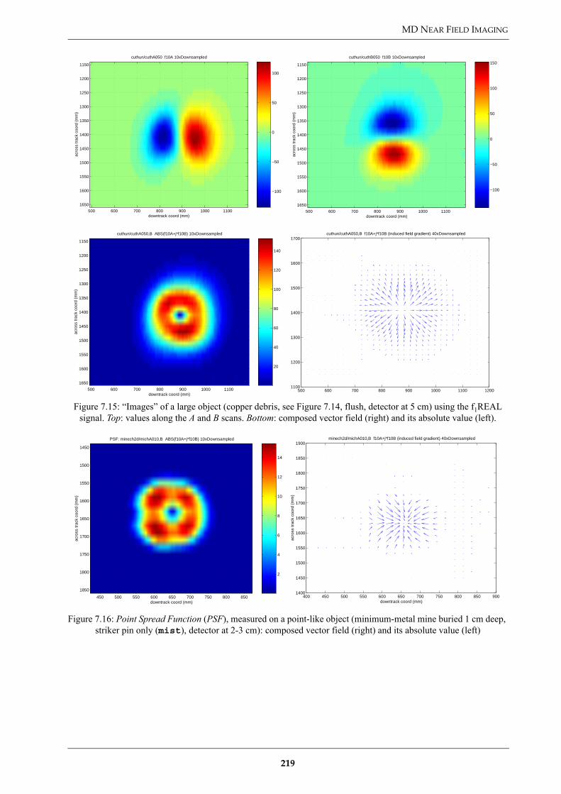
MD NEAR FIELD IMAGING
Figure 7.15: “Images” of a large object (copper debris, see Figure 7.14, flush, detector at 5 cm) using the f1REAL signal. Top: values along the A and B scans. Bottom: composed vector field (right) and its absolute value (left).
Figure 7.16: Point Spread Function (PSF), measured on a point-like object (minimum-metal mine buried 1 cm deep, striker pin only (mist), detector at 2-3 cm): composed vector field (right) and its absolute value (left)
−100
−50
0
50
100
downtrack coord (mm)
acro
ss tr
ack
coor
d (m
m)
cuthun/cuthA050 f10A 10xDownsampled
500 600 700 800 900 1000 1100
1150
1200
1250
1300
1350
1400
1450
1500
1550
1600
1650
−100
−50
0
50
100
150
downtrack coord (mm)
acro
ss tr
ack
coor
d (m
m)
cuthun/cuthB050 f10B 10xDownsampled
500 600 700 800 900 1000 1100
1150
1200
1250
1300
1350
1400
1450
1500
1550
1600
1650
20
40
60
80
100
120
140
downtrack coord (mm)
acro
ss tr
ack
coor
d (m
m)
cuthun/cuthA050,B ABS(f10A+j*f10B) 10xDownsampled
500 600 700 800 900 1000 1100
1150
1200
1250
1300
1350
1400
1450
1500
1550
1600
1650
500 600 700 800 900 1000 1100 12001100
1200
1300
1400
1500
1600
1700cuthun/cuthA050,B f10A+j*f10B (induced field gradient) 40xDownsampled
2
4
6
8
10
12
14
downtrack coord (mm)
acro
ss tr
ack
coor
d (m
m)
PSF: minech2d/michA010,B ABS(f10A+j*f10B) 10xDownsampled
450 500 550 600 650 700 750 800 850
1450
1500
1550
1600
1650
1700
1750
1800
1850
400 450 500 550 600 650 700 750 800 850 9001400
1450
1500
1550
1600
1650
1700
1750
1800
1850
1900
downtrack coord (mm)
acro
ss tr
ack
coor
d (m
m)
minech2d/michA010,B f10A+j*f10B (induced field gradient) 40xDownsampled
219

CHAPTER 7
7.4.2. Deconvolution Results and DiscussionInitial tests have been reported in [BRU98a, BRU98b, BRU00c]. A pseudoinverse filter was usedas previously described, fixing its threshold with a trial and error procedure, with appropriateextensions of the various matrices involved [JAI89,LOW91]. Additional care could reduceboundary related ringing effects, which can be relevant when working with weak signals as theDiscrete Fourier Transform (DFT), used by the deblurring functions, assumes that the frequencypattern of an image is periodic [MAT01].
Typical examples of results are shown in Figure 7.17 and Figure 7.18, together with results fromthe LR algorithm using 10 iterations, no damping and working with the absolute values of theimages.
Figure 7.17 shows results for the same point-like object used to define the PSF; in this case thedeconvolution works quite well at different object depths, although this is certainly favoured bythe fact that in this specific case – basically a small vertical steel nail – the target response doesnot spread out significantly with increasing depth (see Figure 7.4 on the left).
Results are definitely less noisy for the LR algorithm, even for less favourable input data such asat 10 cm (last row, pseudoinverse plot not shown). There is quite good agreement between thetwo filters, although it can be noticed that in the second row the LR algorithm has not yetconverged to the same across track spatial position as the pseudoinverse one (which is here thecorrect one). This is one of the cases in which LR deconvolution results can be improved using ahigher number of iterations.
Figure 7.18 shows results for a couple of realistic, extended objects, the copper debris shown inFigure 7.14, which has an irregular shape and is not flat, and a PMN mine, whose response isdominated by its ring. Larger differences are apparent between the different algorithms, andalthough it is evident that the object has a structure, it is difficult to appreciate its details. Notealso the large halo around the copper debris, which was in fact already present in the initial image(not shown). For these extended objects the LR algorithm results depend much more on thenumber of iterations than for the case of the point-like target.
One example is also shown obtained with a blind deconvolution algorithm, as implemented in theMATLAB® deconvblind function [MAT01], which aims at recovering both the originalimage and the PSF. It has worked in some specialized applications with success, for examplewhen only an imperfect knowledge of the PSF is available. The deconvblind functionperforms deblurring using an iterative process similar to the Lucy-Richardson maximum-likelihood algorithm previously described. In our case the known PSF was provided as initialguess, but results are in general quite inferior to those of the “standard” LR algorithm. A possibleapplication could be the refinement of the PSF when the target depth is not known, but this mightwork only by placing much stronger constraints on the properties of the PSF itself.
Research along similar lines (image deconvolution) has been carried out at the Royal MilitaryAcademy (RMA) in Brussels and is described in [THO98, MER99], with emphasis on Wienerfiltering of amplitude data from a single coil Vallon pulse metal detector. Initial results have thenbeen extensively complemented by the development of a number of target models leading todifferent imaging kernels (PSF) and different interpretations of the target function [DRU00a].The authors have demonstrated that good quality images can be obtained using the rightdeconvolution kernel, i.e. the right target model and the right object depth, which are howeverusually not known a priori. Resolution decreases with depth (good results were obtained up toabout 10 cm).
220

MD NEAR FIELD IMAGING
Figure 7.17: Examples of deconvolved images for a point-like object, a minimum-metal mine buried at 3, 5 and 10 cm (1st, 2nd and 3rd row), striker pin only (mist), detector at 2-3 cm. Left column: pseudoinverse filter, Right
column: Lucy-Richardson maximum likelihood algorithm.
2
4
6
8
10
12
14
16
18x 10
−4
downtrack coord (mm)
acro
ss tr
ack
coor
d (m
m)
Pseudoinverse: minech2d/michA030,B ABS(f10A+j*f10B) 10xDownsampled
400 500 600 700 800 900
1450
1500
1550
1600
1650
1700
1750
1800
18500
0.2
0.4
0.6
0.8
1
1.2
1.4
x 10−3
downtrack coord (mm)
acro
ss tr
ack
coor
d (m
m)
Lucy−Richardson Dec.: minech2d/michA030,B ABS(f10A+j*f10B) 10xDownsampled
400 500 600 700 800 900
1450
1500
1550
1600
1650
1700
1750
1800
1850
0.5
1
1.5
2
2.5
3
3.5
x 10−4
downtrack coord (mm)
acro
ss tr
ack
coor
d (m
m)
Pseudoinverse: minech2d/michA050,B ABS(f10A+j*f10B) 10xDownsampled
400 500 600 700 800 900
1450
1500
1550
1600
1650
1700
1750
1800
18500
1
2
3
4x 10
−4
downtrack coord (mm)
acro
ss tr
ack
coor
d (m
m)
Lucy−Richardson Dec.: minech2d/michA050,B ABS(f10A+j*f10B) 10xDownsampled
400 500 600 700 800 900
1450
1500
1550
1600
1650
1700
1750
1800
1850
0
0.5
1
1.5
2
2.5
3
3.5
4
4.5
x 10−5
downtrack coord (mm)
acro
ss tr
ack
coor
d (m
m)
Lucy−Richardson Dec.: minech2d/michA101,B ABS(f10A+j*f10B) 10xDownsampled
400 500 600 700 800 900
1450
1500
1550
1600
1650
1700
1750
1800
1850
221

CHAPTER 7
Figure 7.18: Examples of deconvolved images for extended objects: copper debris (Figure 7.14) placed perpendicular to the scanning direction (flush) and PMN mine (@1 cm); detector at 5 cm. Left col.: pseudoinverse
filter, Right col.: Lucy-Richardson maximum likelihood algorithm (last image: blind deconvolution).
0.005
0.01
0.015
0.02
0.025
downtrack coord (mm)
acro
ss tr
ack
coor
d (m
m)
Pseudoinverse: cuthun/cuthA050,B ABS(f10A+j*f10B) 10xDownsampled
500 600 700 800 900 1000 1100
1150
1200
1250
1300
1350
1400
1450
1500
1550
1600
1650 0
0.002
0.004
0.006
0.008
0.01
0.012
downtrack coord (mm)
acro
ss tr
ack
coor
d (m
m)
Lucy−Richardson Dec.: cuthun/cuthA050,B ABS(f10A+j*f10B) 10xDownsampled
500 600 700 800 900 1000 1100
1150
1200
1250
1300
1350
1400
1450
1500
1550
1600
1650
0.005
0.01
0.015
0.02
0.025
0.03
0.035
downtrack coord (mm)
acro
ss tr
ack
coor
d (m
m)
Pseudoinverse: PMN ABS(f10A+j*f10B) 10xDownsampled
900 1000 1100 1200 1300 1400 1500
1400
1450
1500
1550
1600
1650
1700
1750
1800 0
0.005
0.01
0.015
downtrack coord (mm)
acro
ss tr
ack
coor
d (m
m)
Lucy−Richardson Dec.: PMN ABS(f10A+j*f10B) 10xDownsampled
900 1000 1100 1200 1300 1400 1500
1400
1450
1500
1550
1600
1650
1700
1750
1800
50
100
150
200
250
300
350
400
450
downtrack coord (mm)
acro
ss tr
ack
coor
d (m
m)
Blind Deconvolution: PMN ABS(f10A+j*f10B) 10xDownsampled
900 1000 1100 1200 1300 1400 1500
1400
1450
1500
1550
1600
1650
1700
1750
1800
222

MD NEAR FIELD IMAGING
7.4.3. ConclusionsStandard metal detectors have not been conceived as imaging devices. As as consequenceunprocessed images are too coarse and unsuitable for direct interpretation, unless large objectsare encountered (of the order of the detector diameter).
Image resolution can be enhanced with deblurring (deconvolution) techniques, as demonstratedin the previous figures. The resulting resolution could at present be sufficient to distinguish point-like from extended or composite objects, which could be useful in a number of scenarios.Improvements can come from a finer sampling of the PSF in the across track direction forexample.
Tuning of the deconvolution algorithms is however not always straightforward, in particular inthe presence of noise, and the resulting images can present artifacts. Also, application of themethod to a portable device will require the use of a precise scanning pattern (probably with highspatial resolution), if possible controlling in some way the detector distance from the surface.Sampling on an irregular grid will also have to be addressed [DRU00a].
Practical applicability will also have to address two basic issues, namely the PSF choice – the useof an “average PSF” is far from optimal according to [DRU00a] – and deviations from the linearmodel assumed in Eq. (7.1), which are likely for ferromagnetic objects.
223

CHAPTER 7
7.5. Conclusions
As a complementary approach to the one described in the previous chapter we have investigatedtwo portable high resolution applications which exploit the geometrical properties of the nearfield, with the aim of understanding if such systems could be useful to provide the deminer with avisual image of the shape and size of the metal signature. The first approach features acommercial multisensor systems designed for NdT applications in civil engineering, the secondconcentrates on the application of image deblurring techniques (deconvolution) to bidimensionaldata obtained with a commercially available sensor, the Förster Minex metal detector.
Concerning the first approach, to the best of our knowledge the first high resolution 2D near real-time “images” of (ferromagnetic) metallic components of mines with relevant metal content (e.g.PMN) and UXO were obtained. They demonstrate that some simple, near real-time highresolution imaging (R=2-3 cm for a flush object) is possible for shallowly buried large orextended targets. Spatial resolution and depth penetration do nevertheless constitute conflictingrequirements, and depth penetration improvements seem necessary for practical applications.
Concerning the second approach, first deconvolved MD images of minelike objects wereobtained using bidimensional data taken with a differential metal detector designed for deminingapplications96, and we demonstrated that image resolution can be enhanced with deblurring(deconvolution) techniques. However, when looking at realistic, extended objects it is evidentthat the target has a structure but it is still difficult to appreciate its details. The resultingresolution could therefore at present be sufficient to distinguish point-like from extended orcomposite objects, which could be useful in a number of scenarios.
This approach has the advantage of using an existing sensor with its well known sensitivity.Tuning of the deconvolution algorithms is however not always straightforward. Also, practicalapplicability will have to address basic issues such as the PSF choice, the use of a precisescanning system, and deviations from the linear model assumed in Eq. (7.1), which are likely forferromagnetic objects.
Improvements in both techniques are obviously possible and have been detailed in thecorresponding paragraphs.
Whether this approach will be practically applicable in the field, from the point of view of theresulting resolution, scanning speed and cost for example, remains to be demonstrated. This willalso depend on whether simpler methods, relying for example on the exploitation of theinformation from traditional metal detectors along the lines described in the previous chapters,will prove to be feasible. In the end it depends therefore on the real added value that such anapproach can bring.
96. As already mentioned similar activities started in parallel at the RMA in Brussels and have been developed since.
224

MD NEAR FIELD IMAGING
Bibliography
[BAH88]Bahr, A. J., and Auld, B. A., 1988, An Electromagnetic Model for Eddy-Current Imaging.Journal of Nondestructive Evaluation, v. 7, no. 1/2, p. 71-77.
[BOR96] Borgwardt, C. High-Precision Mine Detection with Real Time Imaging. Proceedings SPIE No.2765, Conference on Detection and Remediation Technologies for Mines and Minelike Targets,Orlando, FL, USA, Apr. 1996, pp. 301-309.
[BRO96] Brown D.R., et al., “Multisensor Vehicular Mine Detection Testbed for HumanitarianDemining”, in Proc. of the “Technology and the Mine Problem Symposium”, NavalPostgraduate School, Monterey, California, 18-21 Nov. 96., pp. 4-73/4-78.
[BRO98] Brooks, J.; Nicoud, J.D. Applications of GPR Technology to Humanitarian DeminingOperations in Cambodia: Some Lessons Learned. Proceedings of the Third Annual Symposiumon Technology and the Mine Problem, Naval Postgraduate School, Monterey, CA, USA, 6-9Apr. 1998. Available online as ref. Brooks98a at http://diwww.epfl.ch/lami/detec/
[BRU97b]C. Bruschini, “Evaluation of a Commercial Visualizing Metal Detector for UXO/MineDetection: the HILTI Ferroscan System”, SusDem'97 (International Workshop on SustainableHumanitarian Demining) conference poster, Zagreb (Croatia), 29 September-1 October 1997.
[BRU98a]C. Bruschini, B. Gros, F. Guerne, P.-Y. Pièce, and O. Carmona, “Ground penetrating radar andimaging metal detector for antipersonnel mine detection”, J. of Applied Geophysics 40, pp. 59-71, 1998.
[BRU98b]C. Bruschini, “Förster Documentation Overview: Part I: Matlab Algorithms; Signals and DataAcquisition Format (8 pp.); Part II: Metal Detector Test Data (58+6 pp); Part III: 2DDeconvolution Tests (12 pp.)”, EPFL-LAMI and VUB-ETRO-IRIS, Internal Note, Lausanne,Switzerland, April 1998.
[BRU98c]C. Bruschini, “Evaluation of a Commercial Visualizing Metal Detector for UXO/MineDetection: the HILTI Ferroscan System”. Published in Sustainable Humanitarian Demining:Trends, Techniques and Technologies, Mid Valley Press, Verona, VA, USA, Dec. 1998, pp.314-325 ([email protected]).
[BRU00a]C. Bruschini, “Metal detectors in civil engineering and humanitarian de-mining: overview andtests of a commercial visualising system”, INSIGHT – Non-Destructive Testing and ConditionMonitoring 42(2), pp. 89-97, February 2000. Also available from http://diwww.epfl.ch/lami/detec/.
[BRU00c]C. Bruschini, H. Sahli, “Phase angle based clutter reduction and 2D imaging using data from acommercial differential two frequency EMI system”, EUROEM2000 Conference(EuroElectromagnetics), Edinburgh, Scotland, 30/5-2/6 2000, Abstract # 66.5, p. 90.
[CHA00]Chaiken, A. Apparatus and Method for Imaging Metallic Objects using an Array of GiantMagnetoresistive Sensors. US Patent # 6,124,712, 26 Sept. 2000.
[COL84] H. Dale Collins, J. M. Prince, and T. J. Davis. Non-Destructive Testing Method and ApparatusUtilizing Phase Multiplication Holography. US Patent # 4,476,434, 9 Oct. 1984.
[CZI96] Czipott, P.V.; Iwanowski, M.D. Magnetic sensor technology for detecting mines, UXO, andother concealed security threats. Proceedings SPIE No. 2933, Conference on Terrorism andCounterterrorism Methods and Technologies, Boston, MA, USA, 20-21 Nov. 1996, pp. 67-76.
[DAS90] Y. Das, J. E. McFee, J. Toews, and G. C. Stuart, “Analysis of an Electromagnetic InductionDetector For Real-Time Location of Buried Objects”, IEEE Trans. on Geoscience and RemoteSensing, vol. 28, no. 3, pp. 278-288, May 1990.
[DRU00a]P. Druyts, L. Merlat, and M. Acheroy, “Modeling Considerations for Imaging with a StandardMetal Detector”, in Detection and Remediation Technologies for Mines and Minelike Targets;SPIE Proceedings Vol. 4038, pp. 1431-1451, Orlando, FLA, USA, April 2000.
[EBL96] Eblagh, K. Practical Problems in Demining and Their Solutions. Proceedings, EUREL Int.Conference on The Detection of Abandoned Landmines, Edinburgh, UK, 7-9 Oct. 1996, pp. 1-
225

CHAPTER 7
5.[ESC96] Eschner, W.; et al. Bildgebendes hochauflösendes Sensorsystem zu Detektion, Ortung und
Identifizierung von metallischen Objekten (Sensor System for Detecting, Locating andIdentifying Metal Objects). German Patent # DE 44 36 078 A1, 11 Apr. 1996 (in German). Seealso WO96/11414 (international application published under the Patent Cooperation Treaty).
[FER00] Fernandes, B. T., Silva, I., and Gaydecki, P., 2000, Vector extraction from digital images ofsteel bars produced by an inductive scanning system using a differential gradient methodcombined with a modified Hough transform. NDT&E International, v. 33, no. 2, March, p. 69-75.
[GAY94]Gaydecki, P.A.; Burdekin, F.M. An inductive scanning system for two-dimensional imaging ofreinforcing components in concrete structures. Measurement Science and Technology 5, 1994,pp. 1272-1280.
[GAY95]Gaydecki, P.A.; Klossop, K.; Burdekin, F. A prototype inductive scanning system for two-dimensional imaging of metal reinforcing components in concrete: system design and datavisualization. Proceedings, Int. Symposium on Non-Destructive Testing in Civil Engineering,Berlin, Germany, Sept. 1995, pp. 745-752. Online documentation available at http://www.in.umist.ac.uk/DIAS/gaydecki.htm.
[GAY00]Gaydecki, P., Silva, I., Fernandes, B. T., and Yu, Z. Z., 2000, A portable inductive scanningsystem for imaging steel-reinforcing bars embedded within concrete. Sensors and Actuators A(Physical), v. A84, no. 1-2, Aug., p. 25-32.
[GER96] Gerhold, T.; Becker, W.-J.; Ricken, W. Mehrfrequenz-Wirbelstrom-Messverfahren zurStrukturerkennung von Stahlbetonbewehrung bei grösserem Abstand. Grundlagen derZerstörungsfreien Prüfung, Berichtsband 55, Fachausschuss Hochschullehrer, Dortmund(MTQ), Germany, 13 Nov.1996 (in German).
[GOL98] Goldfine, N. J.; et al. Magnetometer and Dielectrometer Detection of Subsurface Objects.WO98/30921 A2, 6 Jan. 1998 (international application published under the Patent Cooperation Treaty).
[GOL99] Goldfine, N., et al., “New Quasistatic Magnetic and Electric Field Imaging Arrays andAlgorithms for Object Detection, Identification, and Discrimination”, in SPIE Proceedings Vol.3710, pp. 89-100, Orlando, FLA, April 1999.
[GUO96]Guo, Y.; Nelson, C.V.; White, D.M. 3-D Localization Using A Time-Domain ElectromagneticSystem. Presented at the UXO Forum 1996, Williamsburg, VA, USA, 26-28 Mar. 1996.
[GUO98]Guo, Y., Ko, H. W., and White, D. M., 1998, 3-D localization of buried objects by nearfieldelectromagnetic holography: Geophysics, v. 63, no. 3, May-June, p. 880-889.
[GUO00]Guo, Y., Ko, H. W., and White, D. M. Imaging Objects in a Dissipative Medium by NearfieldElectromagnetic Holography. US Patent # 6,084,412, 4 Jul. 2000.
[HAN97]Hanisch, R. J., White, R. L., and Gilliland, R. L., 1997, Deconvolution of Hubble SpaceTelescope Images and Spectra, in [JAN97], pp. 310-360.
[HIL94] Ferroscan Product Brochure. Hilti Corporation, FL-9494 Schaan, Liechtenstein, 1994.[HIL97a]Ferroscan System FS 10 Operating Instructions. Hilti Corporation, FL-9494 Schaan,
Liechtenstein, 1997.[HIL97b]Ferroscan Data Analysis Software. Hilti Corporation, FL-9494 Schaan, Liechtenstein, 1997.[HIP90] Hippler, J. H., Ermert, H., and von Bernus, L., 1990, Über die Nutzung des Skin-Effekts für
holographische Abbildungsverfahren zur zerstörungsfreien Prüfung metallischer Materialienund Bauteile (On the utilization of the skin-effect for holographic imaging in nondestructiveevaluation of metallic materials and devices): Archiv für Elektronik und Übertragungs-technik(AEÜ), v. 44, no. 4, July-Aug.., p. 257-264 (in German).
[HIP93] Hippler, J. H., Ermert, H., and von Bernus, L., 1993, Broadband holography applied to eddycurrent imaging by using signals with multiplied phases: Journal of Nondestructive Evaluation,v. 12, no. 3, Sept., p. 153-162.
[JAI89] A. K. Jain, Fundamentals of Digital Signal Image Processing, Prentice-Hall International, 1989,
226

MD NEAR FIELD IMAGING
Ch. 8.[JAN97] P. A. Jansson, Deconvolution of Images and Spectra, 2nd ed., Academic Press, 1997, 514 pp.[KOU94]Kousek, K.; et al. Apparatus for Determining Location of an Element of Magnetizable Material
in a Construction Structure. US Patent # 5,296,807, 22 Mar. 1994.[LOW91]A. Low, Introductory Computer Vision and Image Processing, McGraw-Hill, 1991, Ch. 14.
[MAT01]“MATLAB® Image Processing Toolbox User’s Manual”, v. 3.1 (Release 12.1), May 2001.[KIN96] King C. Mine Clearance…in the Real World. Proceedings of the Technology and the Mine
Problem Symposium, Naval Postgraduate School, Monterey, CA, USA, 18-21 Nov. 1996, pp.3-3/3-9.
[McF96] McFee, J.E.; Carruthers, A. A multisensor mine detector for peacekeeping – ImprovedLandmine Detector Concept (ILDC). Proceedings SPIE No. 2765, Conference on Detection andRemediation Technologies for Mines and Minelike Targets, Orlando, FL, USA, Apr. 1996, pp.233-248.
[MER99]L. Merlat, M. Acheroy, “Improving quality of information from metal detectors”, in Proc. 1999ARIS Technical Workshop on Ground Survey for Humanitarian Demining, Brest, France, 26-27 Oct. 1999.
[MIT96] Tsipis K., “Report on the Landmine Brainstorming Workshop of Aug. 25-30, Nov. 96”, Report#27, Program in Science & Technology for International Security, MIT, Cambridge, MA, USA,1996.
[ODIS96]High-Precision Ordnance Detection with the Real-Time Imaging System ODIS. SystemBrochure, Dornier, Daimler-Benz Aerospace, 1996.
[RIC95] Ricken, W.; Mehlhorn, G.; Becker, W. Determining of the concrete cover thickness and the bardiameter in reinforced concrete with a method of eddy current testing. Proceedings, Int.Symposium on Non-Destructive Testing in Civil Engineering, Berlin, Germany, Sept. 1995, pp.197-204. Online documentation available at http://www.uni-kassel.de/fb16/ipm/mt/de/forschung/mfid/mfid.ghk.
[RUS99] K. Russell, Y. Das, J. McFee, and R. Chesney, “A realtime target detection technique for metaldetector arrays - an image processing approach”, in SPIE Proceedings Vol. 3710, pp. 887-894,Orlando, FLA, April 1999.
[SMI99] G. S. Smith, R. F. Apfeldorfer, and L. E. Rickard Petersson, “The role of evanescentelectromagnetic waves in the detection and identification of buried landmines”, in SPIEProceedings Vol. 3710, pp. 101-112, Orlando, FLA, April 1999.
[SWE97]Swedlow, J. R., Sedat, J. W., and Agard, D. A., 1997, Deconvolution in Optical Microscopy, in[JAN97], pp. 284-309.
[THO98] O. Thonnard, “Détecteur de Métaux – Analyse d’un Détecteur de Métaux et Conception d’unSystème de Balayage afin de Produire des Images 2-D du Sol” (Metal Detector – Analysis of aMetal Detector and Design of a Scanning System for the Generation of 2-D Soil Images),Signal Image Centre, École Royale Militaire (Royal Military Academy), Brussels, Belgium,1998 (M.Sc. Thesis, in French).
[TRI96] Trinkhaus, H.-P.; et al. Verfahren und System zur Altlastendetektion. German Patent # DE 44 23623 A1, 1 Nov. 1996 (in German). See also Eschner, W.; et al. Process for Detecting MetallicItems Including a Search Path Defined by a Linear Movement with a Superimposed RotationalMovement along a Curved Closed Path. US Patent # 5,719,500, 17 Feb. 1998.
[WOL99]Wold, R. J., et al., “Development of a Hand-held Mine Detection System using aMagnetoresistive Sensor Array”, in SPIE Proceedings Vol. 3710, pp. 113-123, Orlando, FLA,April 1999.
227

CHAPTER 7
228

8. Conclusions and Outlook
This thesis has detailed an analysis of metal detectors (low frequency EM inductiondevices) and their use in a number of disciplines (multidisciplinary approach), fromthe technical point of view as well as looking at the underlying basic physics.Frequency Domain (FD) systems and the operational conditions of interest tohumanitarian demining have been emphasized.
An initial look at humanitarian demining and related R&D has allowed to identifyneeds and opportunities for the study of metal detectors. After a review of their basicprinciples we have turned our attention to electromagnetic induction modelling and toanalytical solutions to some basic FD problems, with the aim of understanding thedirect (forward) problem. This sets the theoretical framework. The first chaptershave in fact a tutorial nature as well, as for quite some time little scientificinformation has been available on this subject.
The second half of the thesis focuses on the analysis of an extensive amount of data,following a pattern recognition approach. The possibility of target classification isfirst discussed on a qualitative basis (complex plane plots), then quantitatively(feature definition, extraction and analysis). The experimental data is also comparedto theoretical expectations. Finally, we discuss a complementary approach, i.e. shapeand size determination via near field imaging.
On the theoretical side we emphasized the operating conditions prevailing in humanitariandemining and the phase response of FD systems in particular. We have confirmed the possibilityof distinguishing between different objects and of identifying some targets based on theircharacteristic phase response. In addition, we have indicated the possibility of exploiting thephase shift dependence on the object size to reduce the amount of detected clutter. Finite lengthpermeable cylinders have been considered in a semi-quantitative way and demagnetizationeffects stressed. Finally, we have also considered some second order effects such as galvaniccurrents or the influence of a conductive medium or overburden.
The importance of soil effects (for FD systems in particular), which are often not sufficientlyconsidered in the existing scientific literature, has been recognized early on, in particular forsmall or deep targets. Soil effects have been taken into account by studying the response fordifferent soil permeabilities (homogenous half-space model) and by analysing some frequencydifferencing methods and features which are more robust to variations in ground conditions.Fluctuations in the soil signal are also clearly documented in the experimental data.
On the experimental side we have exploited spatial high-resolution scanning to analyse theresponse from reference objects and targets, ranging from a minimum-metal mine and itscomponents to larger metallic mines and UXO. We have also carried out a detailed clutter(debris) analysis used representative objects. The use of “only” two frequencies is partiallycompensated by them being placed towards the limits of the frequency band of interest.
A number of theoretical elements of the basic models we looked at have been confirmed, inparticular the trends in the phase response with increasing object size and/or conductivity(actually increasing induction number), the difference between ferromagnetic and non-ferromagnetic objects, and important demagnetization effects.
Where we see particular added value for the scientific community is in the detailed responseanalysis, which has allowed to highlight a number of effects such as orientation dependencies orchanges due to axial offsets (elongated ferromagnetic targets). Subtle effects have also been
229

CHAPTER 8
documented, such as the response of composite objects and their variability, or of differentversions of a same mine. This has also been achieved thanks to the use of internal signals, whoseavailability from existing systems was in no way granted at the time this work started.
On the qualitative side (signal trajectories in the complex plane) we have shown that it ispossible to distinguish smaller clutter items from larger objects, and that some mines have quitecharacteristic responses (e.g. PMN). A “qualitative” (coarse) target classification is thereforepossible, at least for situations with a sufficient signal to noise (S/N) ratio.
On the quantitative side we have simplified the complex plane curves by extracting acorresponding set of features, resulting in a combined, simplified user interface. Additionalfeatures have also been proposed and the resulting distributions analysed. Most of the informationturns out to be contained in the phase response; there are however situations in which theadditional features help in resolving ambiguities.
The resulting classification opportunities have then been discussed along three main lines:• A coarse target classification according to the object size (actually the response parameter, see
§6.3), and permeability (ferromagnetic or not), seems indeed to be possible, at least for scenarioswith a sufficient S/N ratio. In the low S/N case it should however still be possible to exploit someof the additional features which are more robust to background (soil) fluctuations.
• The results for some large metallic objects confirm that it is possible to discriminate them forsmaller clutter relying on their phase response. This seems true to a limited extent only for mineswith an average metallic content (e.g. PMN, PMN2).
• Discriminating mines from clutter or among themselves depends in the end on i) which and howmany types of mines are present (a priori knowledge), ii) how much one can rely on stable minesignatures, iii) how representative the debris we had available is, and in particular on iv) how manyclutter objects have a sufficient S/N ratio to allow discrimination. Indeed, the actual system effectiveness will depend on how much the false alarm rate can bereduced, i.e. how many times a clutter item has a sufficient S/N to be identified as such.
Finally, we have shown, to the best of our knowledge, the first high resolution (R=2-3 cm for aflush object) 2D near real-time “images” of shallowly buried (ferromagnetic) metalliccomponents of mines with relevant metal content (e.g. PMN) and UXO. First deconvolved MDimages of minelike objects were also obtained, using 2D data taken with a commercial detectordesigned for demining applications, demonstrating that image resolution can be enhanced withdeblurring (deconvolution) techniques. The limits of both approaches are detailed in Chapter 7.Whether they will be practically applicable in the field, from the point of view of the resultingresolution, scanning speed and cost, remains to be demonstrated.
As a final comment we note that although some of these results were already known to the metaldetector community, their diffusion has rarely happened, to the best of our knowledge, in a publicdocument and in a coherent way, with the necessary scientific rigour.
OutlookAs a next step along the lines of this work it should not be too difficult to move from thelaboratory to the field, in order to acquire data under realistic conditions, learn by looking at theuser interface, and collect preciser target statistics, in particular to understand how many (clutter)objects retain a sufficient S/N ratio for their discrimination. Deceptions can be foreseen fordifficult ground conditions, but that’s part of the learning process. Finally, although emphasis hasbeen put on analytical models it is recognised that it will be beneficial to look at numerical onesto get a more detailed understanding of complex scenarios, to model soil cavities, and possibly toincrease imaging resolution.
Other approaches have already been detailed in the previous chapters and will not be repeatedhere.
230