A Multi-Item Inventory Model With Joint Setup And Concave ...

ERIM REPORT SERIES RESEARCH IN MANAGEMENT ERIM Report Series reference number ERS-2004-044-LIS Publication June 2004 Number of pages 20 Email address corresponding author [email protected] Address Erasmus Research Institute of Management (ERIM)

Rotterdam School of Management / Rotterdam School of Economics Erasmus Universiteit Rotterdam P.O. Box 1738 3000 DR Rotterdam, The Netherlands Phone: +31 10 408 1182 Fax: +31 10 408 9640 Email: [email protected] Internet: www.erim.eur.nl

Bibliographic data and classifications of all the ERIM reports are also available on the ERIM website:

www.erim.eur.nl

A Multi-Item Inventory Model With Joint Setup And

Concave Production Costs

Z.P. Bayındır, S.I. Birbil and J.B.G. Frenk

ERASMUS RESEARCH INSTITUTE OF MANAGEMENT

REPORT SERIES RESEARCH IN MANAGEMENT

BIBLIOGRAPHIC DATA AND CLASSIFICATIONS Abstract The present paper discusses an approach to solve the joint replenishment problem in a

production environment with concave production cost functions. Under this environment, the model leads to a global optimization problem, which is investigated by using some standard results from convex analysis. Consequently, an effective solution procedure is proposed. The proposed procedure is guaranteed to return a solution with a predetermined quality in terms of the objective function value. A computational study is provided to illustrate the performance of the proposed solution procedure with respect to the running time. 5001-6182 Business 5201-5982 Business Science

Library of Congress Classification (LCC) HB 143.7 Optimization Technique

M Business Administration and Business Economics M 11 R 4

Production Management Transportation Systems

Journal of Economic Literature (JEL)

C 61 Optimization Techniques; Programming Models 85 A Business General 260 K 240 B

Logistics Information Systems Management

European Business Schools Library Group (EBSLG)

255 B Decision under constraints Gemeenschappelijke Onderwerpsontsluiting (GOO)

85.00 Bedrijfskunde, Organisatiekunde: algemeen 85.34 85.20

Logistiek management Bestuurlijke informatie, informatieverzorging

Classification GOO

85.03 Methoden en technieken, operations research Bedrijfskunde / Bedrijfseconomie Bedrijfsprocessen, logistiek, management informatiesystemen

Keywords GOO

Voorraadbeheer, optimalisatie Free keywords Inventory, Multi-item, Concave Production Cost, Joint Setup, Lipschitz Optimization,

Concave-Convex Programming

A Multi-item Inventory Model with Joint Setup and

Concave Production Costs

Z. P. Bayındır†, S. I. Birbil ‡, and J. B. G. Frenk†∗

†Econometric Institute, Erasmus University Rotterdam

Postbus 1738, 3000 DR Rotterdam, The Netherlands.

bayindir, [email protected]

‡Erasmus Research Institute of Management, Erasmus University Rotterdam

Postbus 1738, 3000 DR Rotterdam, The Netherlands.

[email protected]

ABSTRACT. The present paper discusses an approach to solve the joint replenishment problem in a

production environment with concave production cost functions. Under this environment, the model

leads to a global optimization problem, which is investigated by using some standard results from

convex analysis. Consequently, an effective solution procedure is proposed. The proposed procedure is

guaranteed to return a solution with a predetermined quality in terms of the objective function value. A

computational study is provided to illustrate the performance of the proposed solution procedure with

respect to the running time.

Keywords. inventory, multi-item, concave production cost, joint setup, Lipschitz optimization, concave-

convex programming

1 Introduction

Inventory planning for multi-item systems with a joint setup cost, is a well-analyzed area of research in

Management Science. The problem is referred to as the joint replenishment problem. The main issue, as

the name suggests, is investigating the economies of scale due to the coordination of the replenished items

that have a common fixed (ordering/setup) cost. Apart from this major fixed cost, there is an individual

minor fixed cost associated with each item. The overall objective is to minimize total average cost by

determining a common basic cycle time along with the ordering frequency for each item. Setting the

ordering frequencies to integer values ensures the coordination of replenishment of items. As a result of

this coordination, savings on the major fixed cost are obtained.

There exists a vast amount of literature on the deterministic joint replenishment problem [see 1–17].

In the literature, one of the main environmental conditionsemployed is the instantaneous replenishment

assumption, which reflects the fact that either items are purchased from an outside supplier or there is

no capacity restriction on the production facility in termsof the production rate. Indeed in a production

∗Corresponding author.

1 June 7, 2004

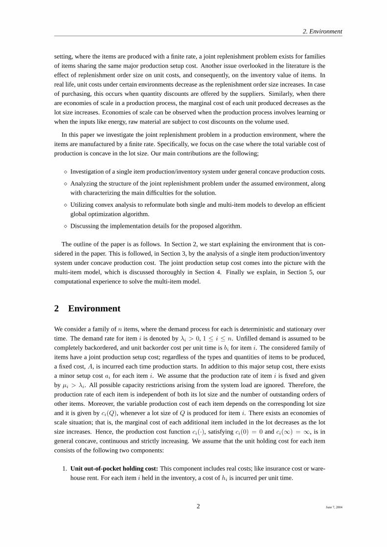
2. Environment

setting, where the items are produced with a finite rate, a joint replenishment problem exists for families

of items sharing the same major production setup cost. Another issue overlooked in the literature is the

effect of replenishment order size on unit costs, and consequently, on the inventory value of items. In

real life, unit costs under certain environments decrease as the replenishment order size increases. In case

of purchasing, this occurs when quantity discounts are offered by the suppliers. Similarly, when there

are economies of scale in a production process, the marginalcost of each unit produced decreases as the

lot size increases. Economies of scale can be observed when the production process involves learning or

when the inputs like energy, raw material are subject to costdiscounts on the volume used.

In this paper we investigate the joint replenishment problem in a production environment, where the

items are manufactured by a finite rate. Specifically, we focus on the case where the total variable cost of

production is concave in the lot size. Our main contributions are the following;

Investigation of a single item production/inventory system under general concave production costs.

Analyzing the structure of the joint replenishment problemunder the assumed environment, along

with characterizing the main difficulties for the solution.

Utilizing convex analysis to reformulate both single and multi-item models to develop an efficient

global optimization algorithm.

Discussing the implementation details for the proposed algorithm.

The outline of the paper is as follows. In Section 2, we start explaining the environment that is con-

sidered in the paper. This is followed, in Section 3, by the analysis of a single item production/inventory

system under concave production cost. The joint productionsetup cost comes into the picture with the

multi-item model, which is discussed thoroughly in Section4. Finally we explain, in Section 5, our

computational experience to solve the multi-item model.

2 Environment

We consider a family ofn items, where the demand process for each is deterministic and stationary over

time. The demand rate for itemi is denoted byλi > 0, 1 ≤ i ≤ n. Unfilled demand is assumed to be

completely backordered, and unit backorder cost per unit time isbi for item i. The considered family of

items have a joint production setup cost; regardless of the types and quantities of items to be produced,

a fixed cost,A, is incurred each time production starts. In addition to this major setup cost, there exists

a minor setup costai for each itemi. We assume that the production rate of itemi is fixed and given

by µi > λi. All possible capacity restrictions arising from the system load are ignored. Therefore, the

production rate of each item is independent of both its lot size and the number of outstanding orders of

other items. Moreover, the variable production cost of eachitem depends on the corresponding lot size

and it is given byci(Q), whenever a lot size ofQ is produced for itemi. There exists an economies of

scale situation; that is, the marginal cost of each additional item included in the lot decreases as the lot

size increases. Hence, the production cost functionci(·), satisfyingci(0) = 0 andci(∞) = ∞, is in

general concave, continuous and strictly increasing. We assume that the unit holding cost for each item

consists of the following two components:

1. Unit out-of-pocket holding cost: This component includes real costs; like insurance cost or ware-

house rent. For each itemi held in the inventory, a cost ofhi is incurred per unit time.

2 June 7, 2004

2. Environment

2. Unit opportunity cost of holding: This component reflects the opportunity cost of tiding up money

into inventories. We consider unit production cost as the cost added to each item. Since unit

production cost depends on the lot size, inventory value of each item included in a certain lot is not

identical. Since it is not possible to differentiate the items physically, the average costing principle

is utilized. Therefore, under the traditional way of setting holding cost rates, when the inventory

carrying charge isr, an opportunity cost ofci(Q)Q

r is incurred per unit time for each itemi produced

in a lot of sizeQ.

An (Si, Ti) type of inventory control rule is considered. According to this rule, the net inventory level

of item i is raised up-to levelSi at everyTi time units. Due to the complete backordering assumption, a

production order ofλiTi is given for itemi at everyTi time periods. The net inventory level under this

policy is depicted in Figure 1.

m -lii-li

Ti

T*

i

Si

net

in

ven

tory

lev

el

timeT =(1- )T

*l ii i/mi

Figure 1: Inventory level for itemi over time.

Using Figure 1, it follows in a cycle of lengthTi and an order-up-to levelSi that the total inventory

and penalty costs in one cycle is given by∫ T∗

i

0

fi(Ti, Si − λit)dt+

∫ Ti−T∗

i

0

fi(Ti, Si − (µi − λi)t)dt, (2.1)

whereT ∗i = (1− λi

µi

)Ti, andfi(·, ·) denotes the so-called cost rate function introduced in [2].After some

easy calculations it follows from relation (2.1) that the total inventory and penalty costs in one cycle is

equal to∫ Ti

0

fi(Ti, Si − σit)dt,

whereσi = λi(1 − λi

µi

). Consequently, if we take into account the minor ordering and production costs,

then the average cost under an(Si, Ti) inventory rule is given by

ai + ci(λiTi) +∫ Ti

0fi(Ti, Si − σit)dt

T.

Hence, in case of a general cost rate function, we have to solve for each itemi, 1 ≤ i ≤ n the optimization

problem

minΦi(Ti) : T > 0, (2.2)

3 June 7, 2004

3. Single Item Production/Inventory Model

where

Φi(Ti) :=ai + ci(λiTi) + φi(Ti)

Ti

(2.3)

and

φi(Ti) := min0≤Si≤σiTi

∫ Ti

0

fi(Ti, Si − σit)dt

.

In this setting, the cost rate function has the form

fi(Ti, x) :=

(hi + ci(λiTi)λiTi

r)x for x ≥ 0

−bix for x < 0.(2.4)

If we introduce the multi-item joint replenishment problemfor the above family, we need to consider

the coordination of these items. In this case, all items havethe same basic cycle timeT and for each

item i production starts within everykiT time units. It is shown by Dagpunar [1], that this boils down to

solving the following optimization problem

min

A∆(k)

T+

n∑

i=1

Φi(kiT ) : T > 0, ki ∈ N

,

where∆(k) denotes the correction factor that keeps track of the empty replenishments. This factor is

given by

∆(k) :=

n∑

i=1

(−1)i+1∑

γ⊂1,··· ,n;|γ|=i

(lcm(kγ1, · · · , kγi

))−1

with lcm(·) denoting the least common multiple of the integer arguments.

Solving now the above problem is complicated due to the correction factor∆(k). Moreover, Goyal

criticizes the formulation of Dagpunar and proposes to set the correction factor equal to one [3]. This

means that the possibility of having empty replenishment occasions are ignored, and so, implicitly there

exists at least one item produced within each basic cycle. This simplifies the problem by setting∆(k) =

1. This approach is followed in many papers (see overviews of Goyal and Satir in [4] and Kaspi and

Rosenblatt in [5]). We therefore rconsider the optimization problem

min

A

T+

n∑

i=1

Φi(kiT ) : T > 0, ki ∈ N

. (2.5)

The model considered in the current study is an extension of asimilar model with linear production

costs discussed in [2, 6]. Contrary to the model in [2, 6], ouranalysis is not related to a special convex

programming problem. It is in general a global optimizationproblem, and this naturally affects our

solution strategy. However, it is still possible to use tools from convex analysis. As a byproduct, we will

show that the optimization problem associated with the inventory control of a single item is actually a

C-programming problem [18]. To start with our analysis, we first present in the next section a detailed

investigation of a single item production/inventory modelwith economies of scale in production.

3 Single Item Production/Inventory Model

In this section we concentrate on the single item production/inventory model introduced in the previous

section. Therefore, the subscripti is suppressed in the subsequent analysis. Recall from relation (2.2) that

for the determination of the optimal policy parameters(S, T ), we need to solve the optimization problem

z1 := minT>0

a+ c(λT ) + φ(T )

T

4 June 7, 2004


with

φ(T ) := min0≤S≤σT

∫ T

0

f(T, S − σt)dt

. (3.1)

Using the specific form of the functionf(·, ·) given in relation (2.4), we obtain by standard arguments

that the optimal solutionS(T ) of the optimization problem in relation (3.1) is given by

S(T ) =bσT

h+ rc(λT )λT

+ b.

Moreover, substitutingS(T ) into (3.1) gives

φ(T ) =b

h+ rc(λT )λT

+ b

(h+ rc(λT )λT

)σT 2

2, (3.2)

and after some simple calculations, this implies

Φ(T ) =a+ c(λT )

T+bσT

2−

λσ(bT )2

2λ(h+ b)T + 2rc(λT ). (3.3)

Consequently, the proposed single item production/inventory problem boils down to the following opti-

mization problem

z1 = minΦ(T ) : T > 0. (P1)

Example 3.1 In case no shortages are allowed (b ↑ ∞), it follows by relation (3.2) that

φ(T ) =(h+ rc(λT )

λT)σT 2

2.

Denoting the objective function for the no shortages case byΨ(·), we obtain

Ψ(T ) =a+ c(λT )

T+σ(hλT + rc(λT ))

2λ, (3.4)

and so, the corresponding optimization problem becomes

z0 := minΨ(T ) : T > 0. (3.5)

Since the production cost functionc(·) is concave, the optimization problem (P1) belongs to the field

of global optimization [19]. Therefore, solving this problem might be quite difficult. We next investigate

whether it is possible to rewrite the problem, and then verify under which additional conditions on the

concave cost functionc(·), problem (P1) can be solved efficiently. To do this, we use the well-known

dual representation of a continuous concave function by means of its biconjugate function. Moreover, in

Section 4 this dual approach will immensely simplify solving the multi-item joint replenishment problem.

In Appendix A we show for everyx ≥ 0 (see Lemma A.1) that

c(x) = infω∈Ω

xω − c∗(ω), (3.6)

whereΩ := [c′−(∞), c′+(0)] is a compact interval withc′−(·) andc′+(·) denoting the left and the right

derivatives of the functionc(·), respectively. Moreover the functionc∗(·) denotes the conjugate ofc(·),

given by

c∗(ω) = infx≥0

ωx− c(x).

Defining the functionF : [0,∞) × (0,∞) → R by

F (x, T ) :=a+ x

T+bσT

2−

λσ(bT )2

2λ(h+ b)T + 2rx, (3.7)

5 June 7, 2004


and using relation (3.3) lead to

Φ(T ) = F (c(λT ), T ). (3.8)

Since the functionx → F (x, T ) is increasing on(0,∞) for everyT , we obtain by relations (3.6) and

(3.8) thatΦ(T ) = F (minω∈ΩλTω − c∗(ω), T )

= minω∈Ω F (λTω − c∗(ω), T ).(3.9)

This implies that problem (P1) can be rewritten as

z1 = minT>0 Φ(T ) = minT>0 minω∈Ω F (λTω − c∗(ω), T )

= minω∈Ω minT>0 F (λωT − c∗(ω), T )

= minω∈Ω minT>0 F (λωT−1 − c∗(ω), T−1).

(3.10)

Note that in the last step we replaced the variableT by T−1. It is easy to see that such a transformation

does not change the optimal objective function value. However, after this simple transformation the inner

minimization problem

minT>0

F (λωT−1 − c∗(ω), T−1), (P1(ω))

becomes a convex optimization problem for eachω ∈ Ω. This is an important observation since comput-

ing the optimal objective function valuez1 requires the solution of problem (P1(ω)) for ω ∈ Ω. We next

give a formal proof of this important observation.

Lemma 3.1 For eachω ∈ Ω the optimization problem (P1(ω)) is a convex programming problem.

Proof. It is easy to compute that

F (λωT − c∗(ω), T ) = λω +a− c∗(ω) + ψω(T )

T

with

ψω(T ) =bσT 2(λ(h+ rω)T − rc∗(ω))

2λ(h+ b+ rω)T − 2rc∗(ω).

Sinceψω(·) is the ratio of a squared convex function (note thatc∗(ω) ≤ 0) and a linear function, it is

convex on(0,∞) [20]. This implies that the functionT → ψω(T−1)T is also convex on the same set

[21]. Consequently, the functionT → F (λωT−1 − c∗(ω), T−1) is convex on(0,∞), and hence the

desired result follows.

Remark 3.1 In Section 4 we will focus on the joint replenishment problem, where the overall optimiza-

tion problem has to be solved for multiple items. The optimalsolution of the problem (P1(ω)) will play

an important role in solving the multi-item (joint replenishment) problem.

As the next example shows, one can give for the no shortages case an analytical expression for the

optimal objective value of the inner optimization problem (P1(ω)).

Example 3.2 If shortages are not allowed (b ↑ ∞), we know by relation (3.4) that the objective function

is given by

Ψ(T ) =a+ c(λT )

T+σ(hλT + rc(λT ))

2λ.

6 June 7, 2004


Using again the dual representation of the cost functionc(·), we can rewrite the optimization problem in

relation (3.5) as

z0 = minT>0

Ψ(T ) = minω∈Ω

minT>0

G(λTω − c∗(ω), T ),

whereG : [0,∞) × (0,∞) → R is given by

G(x, T ) :=a+ x

T+σ(hλT + rx)

2λ.

Now, the corresponding (inner) optimization problem

minT>0

G(λTω − c∗(ω), T )

can be solved analytically with optimal solution valueT (ω) given by

T (ω) =

√

2(a− c∗(ω))

σ(h+ rω).

SubstitutingT (ω) into the objective function yields

G(λT (ω)ω − c∗(ω), T (ω)) = λω −rσc∗(ω)

2λ+a− c∗(ω)

T (ω)+σ(h+ rω)T (ω)

2.

In this case, the overall optimization problem (3.5) becomes

z0 = minω∈Ω

G(λT (ω)ω − c∗(ω), T (ω)).

Before we discuss the general structure of problem (3.10), we introduce the following auxiliary func-

tion

v(ω,−c∗(ω)) := minT>0

F (λωT − c∗(ω), T ) − λω. (3.11)

It is important to note that although the inner problemv(ω,−c∗(ω)) can be computed efficiently, the

overall problem as given by relation (3.10) is, in general, adifficult problem to solve. Nevertheless, the

problem has a special structure that is worth mentioning. InAppendix B, we show in Lemma B.1 that

v(·, ·) is a concave function. Moreover, the arguments of this function ω and−c∗(ω) are both convex

functions. Therefore, the objective function of problem (3.10) is a composition of concave and convex

functions. As a particular subfield of global optimization,C-programming methods are specialized to

find stationary points of such optimization problems [18]. We also note, since the objective function of

the problem is one dimensional, that powerful one dimensional Lipschitz optimization methods can be

applied to solve the problem. One of these approaches will befurther elaborated in Section 5.

As mentioned above solving the overall problem can be quite difficult, unless the cost function pos-

sesses some special properties. In the next example, we illustrate a case where the functionc(·) is poly-

hedral concave;i.e., piecewise linear and concave. In this case solving the overall problem is equivalent

to solving a finite number of convex optimization problems.

Example 3.3 Consider an environment where the production cost functionc(·) is a polyhedral concave

function. This means

c(λT ) := min1≤j≤m

αjλT + βj, (3.12)

whereαm < αm−1 < · · · < α1 and0 = β1 < β2 < · · · < βm (see Figure 2). For the function listed in

(3.12), it is easy to check thatΩ = [c′−(∞), c′+(0)] = [αm, α1]. Moreover, it is well-known thatc∗(·) is

7 June 7, 2004


c(.)

a2

a1

a3

a4

b =01

b2

b3

b4

Figure 2: An example polyhedral concave functionc(·) wherem = 4.

a polyhedral concave function with breaking pointsα1, · · · , αm and so, the functionω → λωT − c∗(ω)

is a polyhedral convex function with the same set of breakingpoints for everyT > 0. Since the function

x→λσ(bT )2

2λ(h+ b)T + 2rx

is convex on(0,∞) for everyT > 0, we obtain by relation (3.7) that the functionx → F (x, T ) is

concave on(0,∞) for everyT > 0. This implies using the polyhedral convexity ofω → λωT − c∗(ω)

with breaking pointsα1, · · · , αm that

minω∈Ω

F (λTω − c∗(ω), T ) = min1≤j≤m

F (λTαj − c∗(αj), T ).

Sincec∗(αj) = −βj , we obtain by relation (3.10) that the overall problem becomes

z1 = min1≤j≤m

λαj + minT>0

a+ βj

T+bσT

2−

λσ(bT )2

2(h+ b+ rαj)λT + 2rβj

.

Notice that solvingm convex optimization problems, and then taking the minimum of their optimum

objective function values givesz1. Moreover, if we also consider the no shortages case (see Example

3.2), then the problem can be solved analytically

z0 = min1≤j≤m

λαj +a+ βj

Tj

+σ(h+ rαj)Tj

2+rσβj

2λ

where

Tj :=

√

2(a+ βj)

σ(h+ rαj).

The polyhedral concave production cost function is frequently used in the literature, especially when

quantity discounting is applied to the cost structure. In fact, it exactly represents the incremental dis-

counting case [22]. It is also important to note that the polyhedral concave functions can be used to

approximate the general concave cost functions.

8 June 7, 2004

4. Multi-item Joint Replenishment Problem

4 Multi-item Joint Replenishment Problem

We are now ready to analyze the multi-item joint replenishment problem (2.5). In this section the subscript

i, ranging from1 to n, is used to denote the items. Before analyzing the problem, we observe that the

multi-item problem (2.5) is separable with respect toki ∈ N for 1 ≤ i ≤ n. Therefore, we can rewrite

the problem as

zn := minT>0

A

T+

n∑

i=1

minki∈N

Φi(kiT )

.

If we further define the functionΘ : [0,∞) → R by

Θ(T ) :=A

T+

n∑

i=1

minki∈N

Φi(kiT ), (4.1)

then the multi-item joint replenishment problem becomes

zn = minΘ(T ) : T > 0. (Pn)

We are now interested in solving the above one-dimensional optimization problem. To achieve this, we

should be able to computeΘ(T0) for any givenT0 > 0, and so, by relation (4.1) we need to solve the

inner optimization problem

minki∈N

Φi(kiT0). (4.2)

Unfortunately, the functionc(·) in relation (2.3) is concave. Therefore, the objective function Φi(·),

in general, does not have a unimodal structure and hence, it might be difficult to solve the problem in

(4.2). A remedy for this problem is to reformulate the functionΦi(·) by the dual approach as done in the

previous section. If we use the subscripti for an item, relation (3.7) is revised as

Fi(x, T ) :=ai + x

T+biσiT

2−

λiσi(biT )2

2λ(hi + bi)T + 2rx, (4.3)

and by relations (3.9) and (4.3), we obtain

Φi(T ) = minω∈Ωi

Fi(λiTω − c∗i (ω), T ). (4.4)

To simplify the exposition of the functionΘ(·), we define the functionHi : Ωi × (0,∞) → R by

Hi(ω, T ) := Fi(λiTω − c∗i (ω), T ). (4.5)

Using now relations (4.1), (4.4) and (4.5) leads to

Θ(T ) = AT

+∑n

i=1minki∈N minω∈ΩiHi(w, kiT )

= AT

+∑n

i=1minω∈Ωiminki∈N Hi(w, kiT ).

(4.6)

If we further denote the optimal solution of the inner optimization problem byki(ω, T ) ∈ N; i.e.,

Hi(ω, ki(ω, T )T ) = minki∈N

Hi(ω, kiT ), (4.7)

then problem (4.2) can be rewritten as

zn = minT>0

Θ(T ) = minT>0

A

T+

n∑

i=1

minω∈Ωi

Hi(w, ki(ω, T )T )

. (4.8)

9 June 7, 2004

4. Multi-item Joint Replenishment Problem

Since we want to evaluateΘ(T0), we should be able to compute for givenω ∈ Ωi the valueki(ω, T0) for

all 1 ≤ i ≤ n. Recall now from Lemma 3.1 that the functionT → Hi(ω, T−1) is a convex function on

(0,∞) for everyω ∈ Ωi, and so, for givenω ∈ Ωi the problem

minT>0

Hi(ω, T−1) (4.9)

is a one-dimensional convex optimization problem. If we denote the optimal solution of problem (4.9) by

Ti(ω) and the optimal solution of problem

minT>0

Hi(ω, T ) (4.10)

by Ti(ω), we obtain thatTi(ω) = 1/Ti(ω). It is clear by the convexity of the functionT → Hi(ω, T−1)

that the functionT → Hi(ω, T ) is increasing forT > Ti(ω) and decreasing forT < Ti(ω). Thus, for

T0 > Ti(ω) it is clear thatki(ω, T0) = 1. On the other hand, forT0 < Ti(ω) we need to find two integers

k−i andk+i (see Figure 3) such that

k−i T0 ≤ Ti(ω) ≤ k+i T0.

This leads to

k−i =

⌊

Ti(ω)

T0

⌋

andk+i =

⌈

Ti(ω)

T0

⌉

, (4.11)

and consequently, for givenT0 > 0, we have

ki(ω, T0) = arg minHi(ω, k−i T0),Hi(ω, k

+i T0). (4.12)

Using relations (4.12) and (4.6), it is easy to evaluateΘ(T0) whenever the setsΩi, 1 ≤ i ≤ n are

finite. In Example 4.1 we demonstrate this observation for the case of polyhedral concave production

cost functions.

T ( )wik Ti

-

0 k Ti 0

+

H (.,.)i

Figure 3: Calculatingki(ω, T0)

Example 4.1 As in Example 3.3, suppose that for each itemi, 1 ≤ i ≤ n, the cost functionsci(·) are

polyhedral concave. This implies that

ci(λiT ) = min1≤j≤mi

αijλiT + βij,

with αimi< αimi−1 · · · < αi1 and0 = βi1 < βi2 < · · · < βimi

. In this special case, the multi-item

joint replenishment problem (4.6) can be written as

zn = minT>0

A

T+

n∑

i=1

min1≤j≤mi

Hi(αij , ki(αij , T )T )

.

Notice that the evaluation ofΘ(T0) for a givenT0 then becomes straightforward, since it only requires∑n

i=1mi calculations to find the values ofHi(αij , ki(αij , T0)T0) for all 1 ≤ j ≤ mi and1 ≤ i ≤ n.

10 June 7, 2004

5. Computational Results

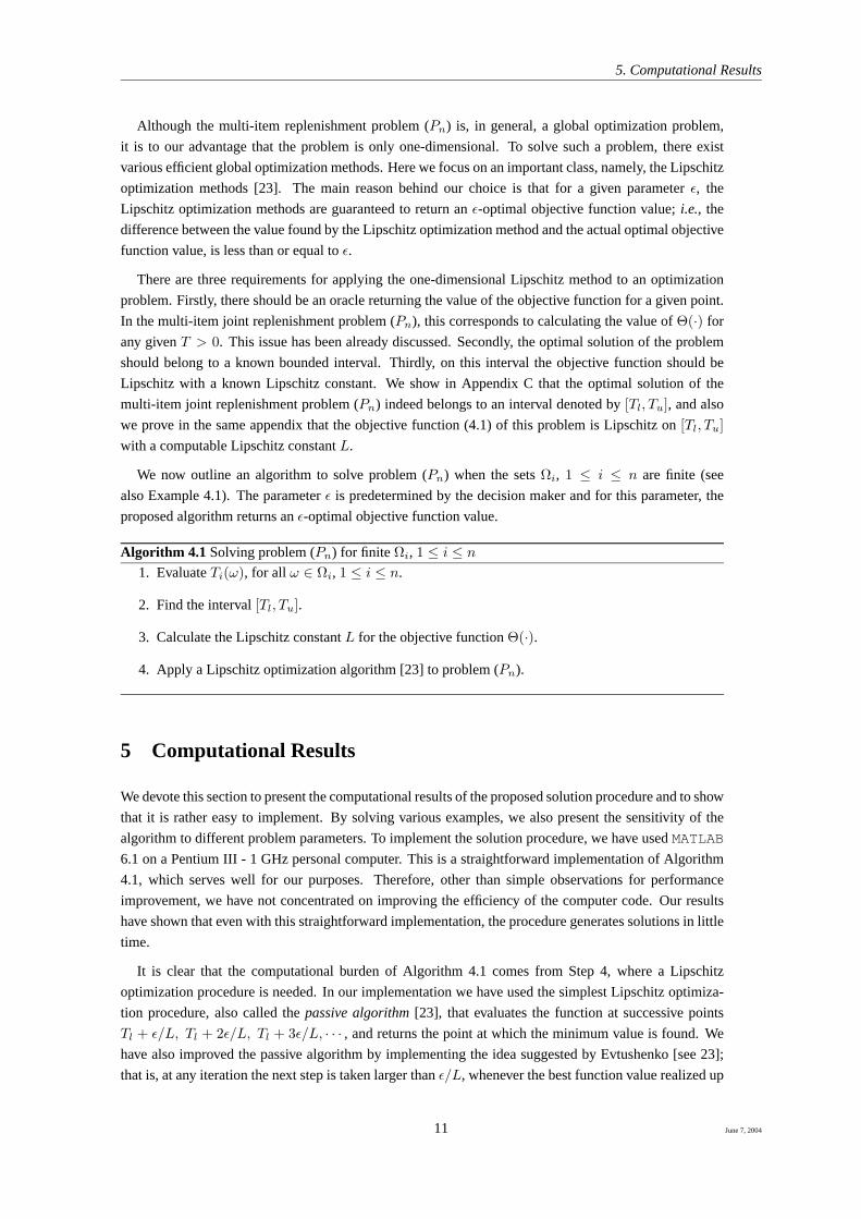
Although the multi-item replenishment problem (Pn) is, in general, a global optimization problem,

it is to our advantage that the problem is only one-dimensional. To solve such a problem, there exist

various efficient global optimization methods. Here we focus on an important class, namely, the Lipschitz

optimization methods [23]. The main reason behind our choice is that for a given parameterε, the

Lipschitz optimization methods are guaranteed to return anε-optimal objective function value;i.e., the

difference between the value found by the Lipschitz optimization method and the actual optimal objective

function value, is less than or equal toε.

There are three requirements for applying the one-dimensional Lipschitz method to an optimization

problem. Firstly, there should be an oracle returning the value of the objective function for a given point.

In the multi-item joint replenishment problem (Pn), this corresponds to calculating the value ofΘ(·) for

any givenT > 0. This issue has been already discussed. Secondly, the optimal solution of the problem

should belong to a known bounded interval. Thirdly, on this interval the objective function should be

Lipschitz with a known Lipschitz constant. We show in Appendix C that the optimal solution of the

multi-item joint replenishment problem (Pn) indeed belongs to an interval denoted by[Tl, Tu], and also

we prove in the same appendix that the objective function (4.1) of this problem is Lipschitz on[Tl, Tu]

with a computable Lipschitz constantL.

We now outline an algorithm to solve problem (Pn) when the setsΩi, 1 ≤ i ≤ n are finite (see

also Example 4.1). The parameterε is predetermined by the decision maker and for this parameter, the

proposed algorithm returns anε-optimal objective function value.

Algorithm 4.1 Solving problem (Pn) for finite Ωi, 1 ≤ i ≤ n

1. EvaluateTi(ω), for all ω ∈ Ωi, 1 ≤ i ≤ n.

2. Find the interval[Tl, Tu].

3. Calculate the Lipschitz constantL for the objective functionΘ(·).

4. Apply a Lipschitz optimization algorithm [23] to problem(Pn).

5 Computational Results

We devote this section to present the computational resultsof the proposed solution procedure and to show

that it is rather easy to implement. By solving various examples, we also present the sensitivity of the

algorithm to different problem parameters. To implement the solution procedure, we have usedMATLAB

6.1 on a Pentium III - 1 GHz personal computer. This is a straightforward implementation of Algorithm

4.1, which serves well for our purposes. Therefore, other than simple observations for performance

improvement, we have not concentrated on improving the efficiency of the computer code. Our results

have shown that even with this straightforward implementation, the procedure generates solutions in little

time.

It is clear that the computational burden of Algorithm 4.1 comes from Step 4, where a Lipschitz

optimization procedure is needed. In our implementation wehave used the simplest Lipschitz optimiza-

tion procedure, also called thepassive algorithm[23], that evaluates the function at successive points

Tl + ε/L, Tl + 2ε/L, Tl + 3ε/L, · · · , and returns the point at which the minimum value is found. We

have also improved the passive algorithm by implementing the idea suggested by Evtushenko [see 23];

that is, at any iteration the next step is taken larger thanε/L, whenever the best function value realized up

11 June 7, 2004


to the current iteration is at leastε above the function value found at the current iteration. Since the values

Ti(ω) andΘ(Ti(ω)) are already calculated in Step 1 and Step 2 of Algorithm 4.1, at the first iteration we

can set the best function value tominΘ(Ti(ω)) : Ti(ω) ∈ [Tl, Tu], 1 ≤ i ≤ n. Moreover, we observe

by relations (C.7) and (C.9) that the Lipschitz constant depends on the valuesTl andTu. Therefore, if

we can partition the interval[Tl, Tu] into subintervals, for each interval we can calculate the correspond-

ing Lipschitz constants and apply the Lipschitz optimization procedure within these subintervals. Notice

that in this case the Lipschitz constants within each interval can be computed by the formulas given in

Appendix C after replacingTl andTu by the lower and upper bounds of the subinterval, respectively. To

partition the interval[Tl, Tu], we can again use theTi(ω) ∈ [Tl, Tu] values found in Step 1. In addition

to Evtushenko’s idea, we have also implemented this simple observation.

As mentioned in the previous section, in real life problems the polyhedral concave functions are used

frequently. Since our main purpose is to illustrate the applicability of the proposed method, we have

generated examples with polyhedral concave cost functions(see Example 4.1).

In the experimental setting we have considered 4 levels for both the number of items,n, and the major

setup cost,A. For every combination ofn andA, 25 problems have been randomly generated. The range

of values for the parameters as well as the levels of the two factors; i.e., n andA, are given in Table

1. Note that except the parametermi, all randomly generated parameters are continuous. The inventory

carrying charge,r has been fixed to 0.15 in all problems. Each generated probleminstance has been

solved under three values of the precision parameterε; 0.1, 0.01, 0.001.

Number of items n ∈ 5, 10, 25, 50

Major setup cost A ∈ 1, 5, 8, 12

Demand rate λi ∼ U(0.1, 5) for 1 ≤ i ≤ n

Production rate µi ∼ U(λi, λi + 5) for 1 ≤ i ≤ n

Minor setup cost ai ∼ U(0.01, 5) for 1 ≤ i ≤ n

Out-of-pocket holding cost hi ∼ U(0.01, 2) for 1 ≤ i ≤ n

Number of breakpoints mi ∼ DU(2, 5) for 1 ≤ i ≤ n

Slopes† αij ∼ U(0.01, 2) for 1 ≤ i ≤ n, 1 ≤ j ≤ mi

Intercepts‡ βi1 = 0 andβij ∼ U(1, 10) for 1 ≤ i ≤ n, 2 ≤ j ≤ mi

Backorder cost bi = hi + 20rαi1 for 1 ≤ i ≤ n

U(lb, ub): Uniform distribution on[lb, ub]

DU(lb, ub): Discrete uniform distribution onlb, ub

† For eachi, 1 ≤ i ≤ n, the valuesαij are sorted in ascending order with respect toj, 1 ≤ j ≤ mi

‡ For eachi, 1 ≤ i ≤ n, the valuesβij are sorted in descending order with respect toj, 2 ≤ j ≤ mi

Table 1: Experimental setting for the factors and the randomly generated parameters.

The raw results of our experimental setting are available upon request. To show the validity of our

results, we have taken 5 problem instances withn = 25. Table 2 shows the optimal objective function

values together with the optimal basic cycle lengths under different major setup cost values. The figures

in Table 2 confirm the basic tradeoff between the major setup cost and the basic cycle time. That is, as the

major setup cost becomes higher, the optimal basic cycle lengths increase. Naturally, the corresponding

cost values also increase.

12 June 7, 2004


Optimal Basic Cycle Length Optimal Average CostInstance A = 1 A = 5 A = 8 A = 12 A = 1 A = 5 A = 8 A = 12

1 2.22 5.69 5.79 6.12 63.66 64.74 65.26 65.93

2 2.46 4.20 4.61 4.82 65.97 67.46 68.11 68.96

3 2.96 5.39 5.49 5.65 62.49 63.48 64.03 64.75

4 1.95 2.85 3.50 4.91 51.99 53.71 54.68 55.69

5 2.51 4.62 5.07 5.17 79.78 80.86 81.46 82.25

Table 2: The results for testing the validity of the proposedprocedure (n = 25, ε = 0.01).

Table 3 gives average running times in seconds (over 25 runs)for each combination ofn, A andε.

As the figures in Table 3 show, no clear effect of the major setup cost on average running times can be

observed. This is due to the fact that although increasingA increases both the lower bound,Tl and the

upper bound,Tu, it may also increase the Lipschitz constants (see AppendixC). However, in many cases,

especially the cases with large number of items, high valuesof A reduces the running time slightly.

On the other hand, increasing the precision and the number ofitems, yields high running times as

expected. Moreover, with respect ton and ε, the growth in the running time is almost linear, and in

all problems the solution is found within less than a minute.At this point, we note that the running

times can be further reduced by efficient implementations. For instance, rewriting the procedure with a

programming language such asC++ could easily improve the performance.

A = 1 A = 5 A = 8 A = 12

ε = 0.1

n = 5 0.64 0.62 1.04 1.64

n = 10 1.44 1.27 1.24 1.22

n = 25 8.85 7.13 6.85 6.91

n = 50 29.46 28.36 27.46 27.33

ε = 0.01

n = 5 1.78 1.05 1.43 2.08

n = 10 2.85 2.28 2.00 1.99

n = 25 18.86 10.00 9.29 8.90

n = 50 42.88 37.39 32.42 32.07

ε = 0.001

n = 5 8.34 2.10 2.39 3.35

n = 10 6.01 4.23 4.61 4.41

n = 25 56.42 17.78 15.89 15.34

n = 50 59.56 55.48 51.27 51.73

Table 3: The average solution times in seconds.

Remember that polyhedral concave functions are frequentlyused in applications for approximating

general concave functions. As the number of affine functions, or equivalently the number of breakpoints,

in the polyhedral concave function increases, the quality of the approximation improves. Therefore, from

a practical point of view it is important to see in which way the number of breakpoints (mi) affect the

performance of the proposed procedure. To test the efficiency of the procedure with respect to varying

number of breakpoints, we have selected three distinct ranges for the discrete uniform distribution. The

values ofA andε are8 and0.01, respectively. For each combination of range andn, 25 problem instances

have been generated using the setting given in Table 1 for theremaining parameters.

13 June 7, 2004


n = 5 n = 10 n = 25 n = 50

mi ∼ DU(2,5) 1.35 1.88 9.58 31.38

mi ∼ DU(6,10) 2.84 6.41 35.40 136.86

mi ∼ DU(11,20) 6.19 18.09 114.56 368.52

Table 4: The average solution times in seconds (A = 8, ε = 0.01).

The average running times are reported in Table 4, where eachrow corresponds to a different range

and each column represents the number of items. It can be seenfrom Table 4 that there is a monotone

relationship between the running time and the number of breakpoints. In addition to increasing the num-

ber of breakpoints, if we also increase the number of items, then the running times grow faster. This

is due to the computational effort invested in the double loops (n by mi) that have to be considered in

the procedure. Nevertheless, using many breakpoints to getfairly accurate approximations, does not cost

much with respect to running time even for the problems with alarge number of items.

14 June 7, 2004

A. Conjugate Function

APPENDIX

A Conjugate Function

Since the functionc : [0,∞) → R is concave, it follows that the functionc(·) is continuous on(0,∞)

and there are only a countable number of points where the function is nondifferentiable. Moreover, for

everyy > 0 both the right derivative

c′+(y) := limx↓y

c(x) − c(y)

x− y

and the left derivative

c′−(y) := limx↑y

c(x) − c(y)

x− y

exist. Also, for everyy1 > y2 > 0 it holds that

c′+(y1) ≤ c′−(y1) ≤ c′+(y2) (A.1)

and the functionsc+(·) andc−(·) are right and left continuous on(0,∞), respectively. By the mono-

tonicity property, expressed in relation (A.1), this implies thatc′+(0) := limy↓0 c′+(y) and c′−(∞) =

limy↑∞ c′−(y) exist and for everyy > 0 it follows that

c′−(∞) ≤ c′+(y) ≤ c′+(0). (A.2)

Since it is also well-known that

c(x) − c(s) =

∫ x

s

c′+(z)dz

for everyx > 0 ands > 0 [24] and0 = c(0) = lims↓0 c(s), we obtain by relation (A.2) and a limiting

argument (takes ↓ 0) that

c(x) ≥ c′−(∞)x (A.3)

for everyx > 0. Introducing now for the concave functionh : R → [−∞,∞), its so-called conjugate

functionh∗ : R → [−∞,∞] given by

h∗(ω) := infωx− h(x) : x ∈ R,

one can show the following dual representation for the function c(·).

Lemma A.1 If c : [0,∞) → R is a concave function satisfying0 = c(0) = limx↓0 c(x), then it follows

for everyx ≥ 0 that

c(x) = infωx− c∗(ω) : c′−(∞) ≤ ω ≤ c′+(0)

with c∗(·) the conjugate function ofc(·) reduced to

c∗(ω) = infωx− c(x) : x ≥ 0.

Proof. Extending the concave functionc : [0,∞) → R to R by introducingc(x) = −∞ for everyx < 0

the extended functionc : R → [−∞,∞) is also concave onR. Moreover, sincec is continuous on(0,∞)

andc(0) = limx↓0 c(x), the upper level sets

U(c, s) := x ∈ R : c(x) ≥ s

15 June 7, 2004

B. Structure of Problem (3.10)

are closed for everys ∈ R and so the extended functionc : R → [−∞,∞) is also upper semicontinuous.

Hence we may apply the biconjugate or Fenchel-Moreau theorem [25] and so it follows that

c(x) = infωx− c∗(ω) : ω ∈ R. (A.4)

Looking now at the conjugate functionc∗(·) of c(·) we obtain due toc(0) = 0 thatc∗(ω) ≤ 0 for every

ω and this shows usingc(x) = −∞ for x < 0 andc∗(ω) ≤ 0 for everyω, that

c∗(ω) = infωx− c(x) : x ≥ 0.

Also, if ω < c′−(∞), it follows by relations (A.3) and (A.4) thatc∗(ω) ≤ ωx − c(x) ≤ (ω − c′−(∞))x

for everyx > 0 and soc∗(ω) = −∞ for everyω < c′−(∞). Moreover ifω > c′+(0) we obtain by the

subgradient inequality for convex functions that

ωx− c(x) ≥ (ω − c′+(0))x

for everyx ≥ 0 and so0 ≥ c∗(ω) ≥ inf(ω − c′+(0))x : x ≥ 0 = 0. Substituting this in relation (A.4)

and usingc(·) is finite on[0,∞) the desired representation follows.

B Structure of Problem (3.10)

Lemma B.1 The functionv : [0,∞) × (0,∞) → R (see also relation (3.11)) given by

v(x, y) := minT>0

a+ y

T+bσT

2−

λσ(bT )2

2λT (h+ b+ rx) + 2ry

is a concave function on[0,∞) × (0,∞).

Proof. Let vT : [0,∞) × (0,∞) → R be a real valued function given by

vT (x, y) :=a+ y

T+bσT

2−

λσ(bT )2

2λT (h+ b+ rx) + 2ry.

Clearly for everyT > 0, the function(x, y) → 2λT (h + b + rx) + 2ry is linear and positive on the

convex set[0,∞) × (0,∞). Hence, by Avrielet. al. [20, Corollary 5.18] we obtain that the function

(x, y) →(bT )2

2λT (h+ b+ rx) + 2ry

is convex on[0,∞) × (0,∞). This implies that the functionvT (·, ·) is a concave function on[0,∞) ×

(0,∞). Sincev(·, ·) is a minimum of concave functions, it is also a concave function and thus, the desired

result follows.

C Bounding Interval and Lipschitz Constants

To apply Lipschitz optimization, we should first construct an interval [Tl, Tu] that contains the optimal

solutionT ∗ of problem (Pn). After this construction we need to compute a Lipschitz constant for the

objective function in (4.1) on this interval.

16 June 7, 2004

C. Bounding Interval and Lipschitz Constants

The objective function of the multi-item joint replenishment problem is given by

Θ(T ) =A

T+

n∑

i=1

minki∈N

Φi(kiT ). (C.1)

Before finding the boundsTl andTu, we first select someT0 > 0 and computeΘ(T0). This allows us to

consider the lower level set

L(Θ(T0)) := T : Θ(T ) ≤ Θ(T0).

Clearly the optimal solutionT ∗ belongs toL(Θ(T0)). Recall thatTi(ω) is the optimal solution of problem

(4.10) forω ∈ Ωi, 1 ≤ i ≤ n. Using now relations (4.4) and (4.5) leads to


Hi(ω, T ) ≥ minω∈Ωi

Hi(ω, Ti(ω)) (C.2)

for all T > 0. To compute a lower boundTl for any elementT belonging toL(Θ(T0)), we observe by

relations (C.1) and (C.2) that

A

T+

n∑

i=1

minω∈Ωi

Hi(ω, Ti(ω)) ≤ Θ(T ) ≤ Θ(T0).

Therefore, the lower bound can be computed as

Tl =A

Θ(T0) −∑n

i=1minω∈ΩiHi(ω, Ti(ω))

,

which implies that a larger lower bound can be gained by decreasing the value ofΘ(T0). Since we have

the individual solutionsTi(ω), one possible way is to set

T0 = arg minΘ(Ti(ω)) : ω ∈ Ωi, 1 ≤ i ≤ n.

To compute an upper bound,Tu, we again use the optimal solutionsTi(ω). Since the functionT →

Hi(ω, T ) is increasing forT > Ti(ω), it follows by relation (4.7) thatki(ω, T ) = 1, and hence

Hi(ω, T ) = minki∈N

Hi(ω, kiT ) (C.3)

for everyT > Ti(ω). By relations (4.4) and (4.5), we know for everyT > 0 that


Hi(ω, T ). (C.4)

This implies using (C.3) and (C.4) that

minki∈N Φi(kiT ) = minki∈N minω∈ΩiHi(ω, kiT )

= minω∈Ωiminki∈N Hi(ω, kiT )

= minω∈ΩiHi(ω, T ) = Φi(T )

(C.5)

for everyT > T := maxTi(ω) : ω ∈ Ωi, 1 ≤ i ≤ n. Moreover, sinceT → Hi(ω, T ) is increasing

on [T ,∞) for everyi andω ∈ Ωi, we also obtain that the functionsΦi(·) are increasing on[T ,∞). This

shows that the functionT →∑n

i=1 Φi(T ) is increasing on[T ,∞), and sincelimT→∞ Φi(T ) = ∞ for

every1 ≤ i ≤ n, we can always find someTu > T satisfying

n∑

i=1

Φi(T ) ≥

n∑

i=1

Φi(Tu) ≥ Θ(T0)

17 June 7, 2004

C. Bounding Interval and Lipschitz Constants

for everyT ≥ Tu. Using now relation (C.5) shows

Θ(T ) ≥n

∑

i=1

Φi(T ) ≥ Θ(T0)

for everyT ≥ Tu. Thus, for everyT belonging toL(Θ(T0)) we obtainT ≤ Tu. The value ofTu can be

found by doing a simple line search on[T ,∞).

Next we compute the Lipschitz constant for the objective function (C.1). Suppose thatL0 is the

Lipschitz constant for the functionT → A/T on [Tl, Tu] andLi are the Lipschitz constants for the

functionsT → minki∈N Φi(kiT ), 1 ≤ i ≤ n on the same interval. If we denote now the Lipschitz

constant of the objective function (C.1) on[Tl, Tu] byL, then it is clear that

L = L0 +

n∑

i=1

Li. (C.6)

Since the functionT → A/T is convex and differentiable on[Tl, Tu], the Lipschitz constantL0 is given

by the maximum of its derivative in absolute values on this interval. That is

L0 =A

T 2l

. (C.7)

By relations (4.7) and (C.5), the valuesLi are also the Lipschitz constants for the functionsT →

minω∈ΩiHi(ω, ki(ω, T )T ) on [Tl, Tu]. Recall from relations (4.11) and (4.12) that givenT > 0

⌊

Ti(ω)

T

⌋

≤ ki(ω, T ) ≤

⌈

Ti(ω)

T

⌉

.

This implies forT ∈ [Tl, Tu] that⌊

Ti(ω)

Tu

⌋

≤

⌊

Ti(ω)

T

⌋

≤ ki(ω, T ) ≤

⌈

Ti(ω)

T

⌉

≤

⌈

Ti(ω)

Tl

⌉

.

Therefore, if we define the finite index set

Ki(ω) :=

k ∈ N :

⌊

Ti(ω)

Tu

⌋

≤ k ≤

⌈

Ti(ω)

Tl

⌉

,

then for anyT ∈ [Tl, Tu] we have

minki∈N

Hi(ω, kiT ) = minki∈Ki(ω)

Hi(ω, kiT ).

Consequently, if we denote the Lipschitz constants for the functionsT → Hi(ω, kiT ) byLi(ω, ki), then

by relation (C.5) we obtain

Li = maxω∈Ωi

maxki∈Ki(ω)

Li(ω, ki). (C.8)

To find the Lipschitz constantsLi(ω, ki), 1 ≤ i ≤ n, we need the following auxiliary result.

Lemma C.1 If the functiong : [a, b] → R, a > 0 is differentiable on[a, b] andh(x) := g(x−1) is a

convex function on[1/b, 1/a], then it follows that

| g(x) − g(y) |≤ Lg | y − x |

with the Lipschitz constant

Lg = max(b/a)2 | g′(b) |, | g′(a) |.

18 June 7, 2004

REFERENCES

Proof. Let Lh denote the Lipschitz constant forh(·) on [1/b, 1/a]. Sinceh(·) is a convex function on

[1/b, 1/a], the Lipschitz constant is given by

Lh = max| h′(1/b) |, | h′(1/a) | = max| b2g′(b) |, | a2g′(a) |.

Moreover, forx, y ∈ [a, b] we have

| g(x) − g(y) | =| h(x−1) − h(y−1) |

≤ Lh | x−1 − y−1 |

≤ Lh

xy| x− y |

≤ Lh

a2 | x− y | .

By settingLg := Lh

a2 , the desired result follows.

Notice by Lemma 3.1 that the functionsT → Hi(ω, (kiT )−1) are convex functions. Therefore, by

Lemma C.1 we obtain

Li(ω, ki) = max

kiT2u

T 2l

| H ′i(ω, kiTu) |, ki | H

′i(ω, kiTl) |

(C.9)

Combining now relations (C.6), (C.7),(C.8) and (C.9) givesthe Lipschitz constant for the objective func-

tion of the joint replenishment problem.

References

[1] Dagpunar, J.S. Formulation of a multi-item single supplier inventory problem. Journal of the

Operational Research Society, 33:285–286, 1982.

[2] Frenk, J.B.G., Kleijn, M.J. and R. Dekker. An efficient algorithm for a generalized joint replenish-

ment problem.European Journal of Operational Research, 118(2):413–428, 1999.

[3] Goyal, S.K. A note on the formulation of a multi-item single supplier inventory problem.Journal

of the Operational Research Society, 33:287–288, 1982.

[4] Goyal, S.K. and A.T. Satir. Joint replenishment inventory control: deterministic and stochastic

models.European Journal of Operational Research, 38:2–13, 1989.

[5] Kaspi, M. and M.J. Rosenblatt. The effectiveness of heuristic algorithms for multi-item inventory

systems with joint replenishment costs.International Journal of Production Research, 23:109–116,

1985.

[6] Wildeman, R.E., Frenk, J.B.G. and R. Dekker. An efficientoptimal solution method for the joint

replenishment problem.European Journal of Operational Research, 99(2):433–444, 1997.

[7] van Eijs, M.J.G. A note on the joint replenishment problem under constant demand.Journal of The


[8] Goyal, S.K. Determination of optimum packaging frequency of items jointly replenished.Manage-

ment Science, 21:436–443, 1974.

[9] Ben-Daya, M. and M. Hariga. Comparative study of heuristics for joint replenishment problem.

Omega, International Journal of Management Science, 23:341–344, 1995.

19 June 7, 2004

REFERENCES

[10] Goyal, S.K. and S.G. Deshmukh. A note on ’the economic ordering quantity of jointly replenished

items’. International Journal of Production Research, 31:2959–2962, 1993.

[11] M. Hariga. Two new heuristic procedures for the joint replenishment problem.Journal of The


[12] Kaspi, M. and M.J. Rosenblatt. An improvement of Silver’s algorithm for the joint replenishment

problem.IIE Transactions, 15:264–269, 1983.

[13] Kaspi, M. and M.J. Rosenblatt. On the economic order quantity for jointly replenished items.

International Journal of Production Research, 29:107–114, 1991.

[14] Klein, C.M. and J.A. Ventura. An optimal method for a deterministic joint replenishment inventory

policy in discrete time.Journal of The Operational Research Society, 46:649–657, 1995.

[15] Silver, E.A. A simple method of determining order quantities in joint replenishments under deter-

ministic demand.Management Science, 22:351–361, 1976.

[16] Fung, R.Y.K. and X. Ma. A new method for joint replenishment problems.Journal of The Opera-

tional Research Society, 52:358–362, 2001.

[17] Viswanathan, S. A new optimal algorithm for the joint replenishment problem.Journal of The


[18] Sniedovich, M. C-programming - an outline.Operations Research Letters, 4(1):19–21, 1985.

[19] Horst, R., Pardalos, P.M. and N.V. Thoai.Introduction to Global Optimization. Kluwer Academic

Publishers, Dordrecht, 1995.

[20] Avriel, M. and Diewert, W.E. and Schaible, S. and I. Zang. Generalized Concavity. Plenum Press,

New York, 1988.

[21] Hiriart-Urruty, J.B. and C. Lemarechal.Convex Analysis and Minimization Algorithms, volume 1.

Springer Verlag, Berlin, 1993.

[22] Silver, E.A., Pyke, D.F. and R. Peterson.Inventory Management and Production Planning and

Scheduling. John Wiley and Sons, 1998.

[23] Hansen, P. and B. Jaumard. Lipschitz optimization. In R. Horst and P.M. Pardalos, editors,Hand-

book of Global Optimization, volume 2 ofNonconvex Optimization and Its Applications. Kluwer

Academic Publishers, Dordrecht, The Netherlands, 1995.

[24] Roberts, A.W. and D.E. Varberg.Convex Functions. Academic Press, New York, 1973.

[25] Rockafellar, R.T.Convex Analysis. Princeton University Press, New Jersey, 1972.

20 June 7, 2004

Publications in the Report Series Research∗ in Management ERIM Research Program: “Business Processes, Logistics and Information Systems” 2004 Smart Pricing: Linking Pricing Decisions with Operational Insights Moritz Fleischmann, Joseph M. Hall and David F. Pyke ERS-2004-001-LIS http://hdl.handle.net/1765/1114 Mobile operators as banks or vice-versa? and: the challenges of Mobile channels for banks L-F Pau ERS-2004-015-LIS http://hdl.handle.net/1765/1163 Simulation-based solution of stochastic mathematical programs with complementarity constraints: Sample-path analysis S. Ilker Birbil, Gül Gürkan and Ovidiu Listeş ERS-2004-016-LIS http://hdl.handle.net/1765/1164 Combining economic and social goals in the design of production systems by using ergonomics standards Jan Dul, Henk de Vries, Sandra Verschoof, Wietske Eveleens and Albert Feilzer ERS-2004-020-LIS http://hdl.handle.net/1765/1200 Factory Gate Pricing: An Analysis of the Dutch Retail Distribution H.M. le Blanc, F. Cruijssen, H.A. Fleuren, M.B.M. de Koster ERS-2004-023-LIS http://hdl.handle.net/1765/1443 A Review Of Design And Control Of Automated Guided Vehicle Systems Tuan Le-Anh and M.B.M. De Koster ERS-2004-030-LIS http://hdl.handle.net/1765/1323 Online Dispatching Rules For Vehicle-Based Internal Transport Systems Tuan Le-Anh and M.B.M. De Koster ERS-2004-031-LIS http://hdl.handle.net/1765/1324 Generalized Fractional Programming With User Interaction S.I. Birbil, J.B.G. Frenk and S. Zhang ERS-2004-033-LIS http://hdl.handle.net/1765/1325

∗ A complete overview of the ERIM Report Series Research in Management:

https://ep.eur.nl/handle/1765/1 ERIM Research Programs: LIS Business Processes, Logistics and Information Systems ORG Organizing for Performance MKT Marketing F&A Finance and Accounting STR Strategy and Entrepreneurship

Meta-heuristics for dynamic lot sizing: A review and comparison of solution approaches Raf Jans and Zeger Degraeve ERS-2004-042-LIS http://hdl.handle.net/1765/1336 A Multi-Item Inventory Model With Joint Setup And Concave Production Costs Z.P. Bayındır, S.I. Birbil and J.B.G. Frenk ERS-2004-044-LIS http://hdl.handle.net/1765/1535 The Level Set Method Of Joó And Its Use In Minimax Theory J.B.G. Frenk and G. Kassay ERS-2004-045-LIS http://hdl.handle.net/1765/1537 Reinventing Crew Scheduling At Netherlands Railways Erwin Abbink, Matteo Fischetti, Leo Kroon, Gerrit Timmer And Michiel Vromans ERS-2004-046-LIS http://hdl.handle.net/1765/1427 Intense Collaboration In Globally Distributed Teams: Evolving Patterns Of Dependencies And Coordination Kuldeep Kumar, Paul C. van Fenema and Mary Ann Von Glinow ERS-2004-052-LIS http://hdl.handle.net/1765/1446 The Value Of Information In Reverse Logistics Michael E. Ketzenberg, Erwin van der Laan and Ruud H. Teunter ERS-2004-053-LIS http://hdl.handle.net/1765/1447 Cargo Revenue Management: Bid-Prices For A 0-1 Multi Knapsack Problem Kevin Pak and Rommert Dekker ERS-2004-055-LIS http://hdl.handle.net/1765/1449 Real-Time Scheduling Approaches For Vehicle-Based Internal Transport Systems Tuan Le-Anh and M.B.M. De Koster ERS-2004-056-LIS http://hdl.handle.net/1765/1452 Activating Knowledge Through Electronic Collaboration: Vanquishing The Knowledge Paradox S. Qureshi and P. Keen ERS-2004-058-LIS http://hdl.handle.net/1765/1473 A Grounded Theory Analysis Of E-Collaboration Effects For Distributed Project Management S. Qureshi, M. Liu and D. Vogel ERS-2004-059-LIS http://hdl.handle.net/1765/1448 Collaborative Infrastructures For Mobilizing Intellectual Resources: Assessing Intellectual Bandwidth In A Knowledge Intensive Organization R. Verhoef and S. Qureshi ERS-2004-060-LIS http://hdl.handle.net/1765/1474 Satisfaction Attainment Theory As A Model For Value Creation R.O. Briggs, S. Qureshi and B. Reining ERS-2004-062-LIS http://hdl.handle.net/1765/1450

Diagnosis In The Olap Context Emiel Caron, Hennie Daniels ERS-2004-063-LIS http://hdl.handle.net/1765/1492 A Deterministic Inventory/Production Model With General Inventory Cost Rate Function And Concave Production Costs Z.P. Bayındır, S.I. Birbil and J.B.G. Frenk ERS-2004-064-LIS http://hdl.handle.net/1765/1536

A Multi-Item Inventory Model With Joint Setup And Concave ...

Documents

Transcript of A Multi-Item Inventory Model With Joint Setup And Concave ...