A Multi-domain Co-Simulator for Smart Grid: Modeling Interactions in Power, Control ... ·...

A Multi-domain Co-Simulator for Smart Grid: Modeling Interactions in Power, Control and Communications

by

Mellitus Okwudili Ezeme

A thesis submitted in conformity with the requirements for the degree of Master of Applied Science

Department of Electrical and Computer Engineering University of Toronto

© Copyright by Mellitus Okwudili Ezeme 2015

ii

A Multi-domain Co-Simulator for Smart Grid: Modeling

Interactions in Power, Control and Communications

Mellitus Okwudili Ezeme

Master of Applied Science

Department of Electrical and Computer Engineering University of Toronto

2015

Abstract

Smart grid studies have been generating a lot of interest both in the business and research

community as it is now seen as the future power grid. However, understanding the interactions

amongst different components that form the smart grid is a Herculean task. Researchers rely on

simulations as one of the means of understanding the effects of coupling the distributed control

systems, communication networks and power system to form the smart grid, but synchronization

of the simulation times of the various simulators, and data exchange amongst the different

components are challenges that must be overcome. Fixed-time-step and queuing system

synchronization schemes have been proposed, but the fixed-time-step synchronization scheme

suffers from accumulation errors and the proposed queuing method does not scale well. In this

thesis, we present a synchronization scheme that eliminates accumulated synchronization errors,

and efficient data exchange scheme which enhances the scalability of the platform.

iii

Acknowledgements I am grateful to my family for the emotional and financial support they gave me during this

program. Their enduring love, compassion and encouragement kept me going even when I

questioned my own ability. I am also indebted to my research group members (Eman, Abdallah,

Pirathayini, and Joseph) for sparing their time any time I needed help.

This acknowledgement would not be complete without the mention of my Supervisor, Professor

Deepa Kundur, who I owe so much for giving me the platform to do this degree, and advising me

both like a mother and a professor. I will forever remain indebted to her for allowing me take a

sip from her intellectual cup.

iv

Table of Contents Acknowledgements ........................................................................................................................ iii

Table of Contents ........................................................................................................................... iv

List of Tables ............................................................................................................................... viii

List of Figures ................................................................................................................................ ix

Chapter 1 ......................................................................................................................................... 1

1 Introduction ................................................................................................................................ 1

1.1 Background ......................................................................................................................... 1

1.2 Why co-simulator ................................................................................................................ 4

1.2.1 Synchronization ...................................................................................................... 5

1.3 Literature Review ................................................................................................................ 6

1.4 Statement of the Problem and Research Objectives ......................................................... 11

1.5 Dissertation Layout ........................................................................................................... 12

Chapter 2 ....................................................................................................................................... 14

2 Co-simulation in Smart Grid .................................................................................................... 14

2.1 Smart Grid System ............................................................................................................ 14

2.1.1 Components of Smart Grid ................................................................................... 16

2.2 Smart Grid Co-Simulator .................................................................................................. 17

2.2.1 Types of co-simulator ........................................................................................... 17

2.2.2 Components of smart grid co-simulator ............................................................... 20

2.2.3 Methods of co-simulation ..................................................................................... 23

2.3 Smart grid co-simulator modeling approaches ................................................................. 23

2.3.1 Mathematical models ............................................................................................ 24

2.3.2 Simulation modeling ............................................................................................. 26

2.4 Synchronization in smart grid co-simulation .................................................................... 27

2.4.1 Periodic Synchronization ...................................................................................... 28

v

2.4.2 Event-based Synchronization ................................................................................ 29

2.5 Data Exchange in Smart Grid Simulation ......................................................................... 29

2.5.1 Pipes ...................................................................................................................... 30

2.5.2 Shared Memory ..................................................................................................... 30

2.5.3 Sockets .................................................................................................................. 31

2.6 Tool Sets Discussion ......................................................................................................... 31

2.6.1 PSCAD/EMTDC ................................................................................................... 31

2.6.2 OMNeT++ /INET ................................................................................................. 32

2.6.3 MATLAB/Simulink .............................................................................................. 32

2.7 Applications of Smart Grid multi-domain simulator ........................................................ 33

2.7.1 State Estimation .................................................................................................... 34

2.7.2 Small Signal Stability ........................................................................................... 34

2.7.3 Voltage Stability Analysis .................................................................................... 34

2.7.4 Postmortem Analysis ............................................................................................ 34

2.7.5 Transient Analysis ................................................................................................ 34

2.8 Summary ........................................................................................................................... 35

Chapter 3 ....................................................................................................................................... 37

3 Software Implementation ......................................................................................................... 37

3.1 The Power System Module ............................................................................................... 37

3.1.1 Power System Design in PSCAD ......................................................................... 38

3.1.2 EMTDC and C Interface ....................................................................................... 39

3.2 Energy Management System (EMS) ................................................................................ 42

3.3 Scheduler ........................................................................................................................... 43

3.3.1 Create Table Module () ......................................................................................... 45

3.3.2 Create Default Status () ......................................................................................... 45

3.3.3 Rate Module () ...................................................................................................... 45

vi

3.3.4 Search Send Flag Module () ................................................................................. 45

3.3.5 Socket Module () ................................................................................................... 46

3.3.6 Write Database Module () ..................................................................................... 46

3.3.7 Read Database Module () ...................................................................................... 46

3.3.8 Update Output Module () ...................................................................................... 47

3.4 The Communication System ............................................................................................. 47

3.4.1 OMNeT++ ............................................................................................................ 48

3.4.2 INET Framework .................................................................................................. 48

3.4.3 C++ Interface ........................................................................................................ 52

3.5 Summary ........................................................................................................................... 53

Chapter 4 ....................................................................................................................................... 54

4 Test Cases: Microgrid Control and Communication ............................................................... 54

4.1 Study System: Microgrid .................................................................................................. 54

4.1.1 Power Management .............................................................................................. 57

4.1.2 Frequency Control and Synchronization .............................................................. 58

4.1.3 Local Controllers .................................................................................................. 58

4.2 Communication Architecture ............................................................................................ 59

4.2.1 Geni LAN .............................................................................................................. 60

4.2.2 Energy Management System ................................................................................ 60

4.2.3 Communication Channel ...................................................................................... 61

4.3 Simulation Results ............................................................................................................ 62

4.3.1 Performance metrics ............................................................................................. 62

4.3.2 Single-domain simulation ..................................................................................... 63

4.3.3 Fixed-delay Single-domain simulation ................................................................. 63

4.3.4 Multi-domain simulation ...................................................................................... 64

4.4 Impact evaluation .............................................................................................................. 64

vii

4.4.1 Effect of sampling rate on controller .................................................................... 64

4.4.2 Discussion of results ............................................................................................. 69

4.5 Summary ........................................................................................................................... 73

Chapter 5 ....................................................................................................................................... 75

5 Conclusion ................................................................................................................................ 75

5.1 Summary and Conclusions ............................................................................................... 75

5.2 Challenges and Limitations ............................................................................................... 76

5.3 Contributions ..................................................................................................................... 77

5.4 Future Research Directions ............................................................................................... 77

viii

List of Tables Table 2-1 Synchronization methods in some reviewed works. .................................................... 28

Table 2-2: Smart Grid Applications Classified According to Latency Requirement. .................. 33

Table 2-3: Smart grid co-simulation approaches with the pros and cons of each method ........... 35

Table 4-1 Microgrid Data showing the ratings of the DERs, load and line impedance. .............. 56

Table 4-2: Packet Structure of transmitted data, channel capacity, channel types and their

characteristics ............................................................................................................................... 61

ix

List of Figures Figure 1-1: Continuous-time simulation sequence of PSCAD ....................................................... 3

Figure 1-2 Discrete time simulation depicting the execution of queued events which can jump in

time ................................................................................................................................................. 4

Figure 2-1: Smart grid system showing the renewable and non-renewable energy sources, the

control center, and the communication network overlay............................................................. 16

Figure 2-2: Diagram showing the interaction of the components of the smart grid co-simulator20

Figure 2-3: Interactive co-simulation depicting the bi-directional information exchange. ......... 27

Figure 2-4: Non-interactive co-simulation showing unidirectional flow of information. ............ 27

Figure 3-1: System architecture showing the interconnection of the different components that

make up the smart grid. ................................................................................................................ 37

Figure 3-2: Software Architecture of the Co-simulator with all the key components .................. 38

Figure 3-3: Pseudo code for the dynamic buffer managing traffic from different sources going

into the communication network. .................................................................................................. 40

Figure 3-4: Pseudo code of the dynamic buffer managing traffic reception from the

communication network. ............................................................................................................... 41

Figure 3-5: Flowchart showing the working principle of the scheduler with Communication

Network and EMS as black boxes. ................................................................................................ 44

Figure 3-6 TCP Signaling diagram showing connection establishment, connection maintenance

and connection teardown ............................................................................................................. 50

Figure 4-1 Complete diagram of the study microgrid identifying the loads, the DERs, and the

main grid. ...................................................................................................................................... 56

Figure 4-2 Sawtooth Waveform used to regulate the output of the DERs. .................................. 58

https://d.docs.live.net/58d69afe822da748/Thesis%20material/Ezeme_Mellitus_MASc_thesisfirstdraft-OkwudilChukwu.doc%23_Toc428030874







x

Figure 4-3: Communication system equivalent of the microgrid showing the interconnection

amongst the key components of the system. .................................................................................. 60

Figure 4-4: Single domain simulation showing the response of the DGs to transient instability

(load shedding) ............................................................................................................................. 65

Figure 4-5:Non-interactive simulation showing the response of the DGs to transient instability

(load shedding) ............................................................................................................................. 66

Figure 4-6: Full co-simulation showing the response of the DGs to transient instability (load

shedding) ....................................................................................................................................... 67

Figure 4-7: Real time simulation of the wireless channel and the power components of the DERs

....................................................................................................................................................... 68

Figure 4-8: Non-real time wireless channel simulation and the reaction of the DERs to load

connection and disconnection ...................................................................................................... 69

Figure 4-9: Pseudocode showing the data structure used by the scheduler during

synchronization ............................................................................................................................. 71







1

Chapter 1

Introduction

1.1 Background Virtually every device around us today is becoming “smart.” Even physical infrastructure like

the power grid is not left behind. The advancement of power systems, to provide greater

consumer-centricity, more efficiency and a smaller carbon-footprint, has motivated the need for

power grid cyber-enablement [1]. Cyber-enablement will no doubt enable high fidelity data

acquisition and processing for effective decision-making. However, for the legacy power grid to

become a smart grid, it must undergo system integration with advanced sensors, high speed

communications and distributed control, which present significant challenges. Two non-

functional challenges of information and communication technology ICT integration are

interoperability and cyber security. According to [2], interoperability represents the ease by

which a system can exchange information with another system. For our discussion here, it

suffices to say that interoperability issues increase with the “distance” between the measurement

source and the application. The distance here is not only geographical, but also has a context or

organizational dimension; thus, if data transverses several networks within, or outside a

regulatory scope, additional interoperability issues may be experienced due to protocol

conversions or communication gateways and network configurations. The second non-functional

aspect of ICT integration is cyber security. In [3], cyber security is extensively discussed and

provides the best example of the dangers of focusing ICT development merely on the function to

be fulfilled.

Researchers and engineers aiming to perform this form of integration often must study the

impact of bringing two such systems together, and this again is not easy because of the inherent

diverse nature of the two systems. The power grid exhibits analog system behavior while the

cyber system is discrete in nature. Continuous-time simulators of power systems are considered

to mimic analog behavior because of the use of fixed time-step with no jump in time during the

simulation process. This means that there is an event for every time-step in the simulation. Also,

2

it is worthy of note that the time-step is determined and set by a user based on the features of the

power system being studied. This behavior is illustrated in Figure 1-1. In contrast, as shown in

Figure 1-2, communication simulators that often model queued events typically can jump in time

and employ a varying time-step that is beyond user control. Here, the system determines when an

event is created and determines whether to cancel or execute the event based on the outcome of

previous events.

The distinct characteristics of each type of simulator makes exploration of a cyber-enabled smart

grid difficult within a common existing framework. Hence, there is a need to develop co-

simulators capable of solving the integration challenges while maintaining the independence of

each of the systems under study, which is the topic of this thesis. This usually involves using a

power simulator, a communication simulator and a simulator capable of rigorous control

behavior manipulations if the need arises. Enabling these separate simulators to work together

and still depict acceptable real system behavior involves overcoming the challenges of

synchronization of the simulation times of the simulators, and data exchange amongst the

systems.

The synchronization problem arises because of the nature of the simulators used in the cross-

domain simulation. As highlighted above, most network simulators such as NS21, NS3,

OPNET, OMNeT++, etc., are discrete event simulators. This means that they are driven by

queued events, which occur at a particular time and marks a change of system state. Between two

consecutive events, it is assumed that the system state is unchanged [4]. This makes it possible

for the system to jump over time from one event to the next. On the other hand, power simulators

such as PSCAD2, PSLF3, etc., are continuous-time simulators that solve differential equations at

fixed time-steps. This step by step execution, otherwise known as continuous-time simulation as

cited above, means that every time-step must be accounted for [4]. Hence, in every fixed time-

1 NS2 and NS3 are communication network simulators; NS3 represents a newer version of NS2.

2 Power System Computer Aided Design (PSCAD) is the graphical user interface for the power simulator.

3 Positive Sequence Load Flow (PSLF) is continuous-time power simulator used mostly for load flow studies.

3

step, an event is executed. This difference in simulation time behavior presents a synchronization

problem which is elaborated more in Section 2.4 of this work.

Figure 1-1: Continuous-time simulation sequence of PSCAD

4

The rest of this chapter is organized as follows. Section 1.2 discusses why we need a co-

simulator and plain explanation of synchronization. Section 1.3 reviews the numerous literature

in this field with emphasis on the merits and limitations of each. Section 1.4 presents the

statement of the problem and objectives. Section 1.5 presents the organization of the thesis.

1.2 Why co-simulator In [5], a microgrid system using only a power simulator and assuming zero end-to-end delay is

implemented. Also, in [6], a communication network simulator is used to simulate the

communication needs of a virtual power system. The difference in the simulation domain of the

two systems as highlighted in [7] has made it difficult to use one simulator to accomplish both

needs. But we also note that while most considerations in power systems is via mathematical

equations, the communication system is a stochastic system, and the randomness it introduces in

the overall behavior of cyber-physical system like microgrid can only be captured by using a co-

Figure 1-2 Discrete time simulation depicting the execution of queued events which can jump in time

5

simulator. Hence, the high interest by researchers in this area. The use of co-simulator also

allows us to achieve the following:

• Domain specific modeling: With multi-domain co-simulator, we have the flexibility of

modeling and designing each of the systems involved in the integration in their respective

domain, thereby making our work easier and modular in nature.

• Well-developed simulators: Each of the simulators involved in the integration has

evolved over time and has large research community that keeps developing and

improving the simulators. Hence, it affords us the benefit of having well tested simulators

with known consistent behavior than developing another one from scratch.

• Component reuse: Another benefit of this integration is the ability to reuse components

that have been developed by others in this field. An example is the INET modules in

OMNeT++ which would have been built from scratch if we had to build our own

simulator.

1.2.1 Synchronization

As highlighted in Section 1.1, the behavior of the federating simulators with different execution

method makes modelling the interaction amongst the different entities difficult as the simulation

time of the various simulators involved in the federation are different. Hence, the co-simulation

design tries to model the practical behavior of the systems involved by ensuring that events are

applied at exactly when they are supposed to happen in reference to the time-stamp. Processing

times by sensors and actuators, propagation and transmission delays incurred by communication

systems all affect the true behavior of the co-simulated system. Hence, application of an event

with a time-stamp less than the simulation time will halt the simulation prematurely, and

triggering an event before the simulation time introduces an error to the modelling process.

Therefore, synchronization is a process of harmonizing the simulation time of the federating

simulators to ensure that events are applied according to their time-stamps without halting the

simulation prematurely or accumulating errors, thereby depicting the behavior of the modelled

systems closely.

6

1.3 Literature Review For the past two decades, there has been growing interest in the development of a smart grid

system as evidenced by the literature in this area [4, 6-16]. However, the topic of smart grid

(power-communications-control) multi-domain simulation remains an open field of study, to the

best of the knowledge of the author. In this section, we will highlight some research that is

closely related to the work in this thesis.

The earliest approach is entitled MESCOS ̶ A Multi-energy System Co-simulator for City district

Energy Systems [17] which is a multi-domain simulation platform that analyzes city district

energy systems with the aim of serving as a tool for the design and control of energy

management systems. By multi-domain, the author refers to the fact that the integrated

simulators can simultaneously run power system and rigorous control system analyses required

for efficient power system management. The work claims to take into account the various

internal and external sources available for city-scale energy systems, including internal

conversion systems and electrical grids. Moreover, the authors state the work can provide

analysis for a variety of energy sources like solar, wind, biogas and the main grid, which is a

positive feature given that the smart grid requires integration of both the traditional power

sources and distributed energy resources (DER’s)4 [18]. The work however does not take into

account the effect of the communication network infrastructure needed to coordinate the

operation of the both the energy management system and the actuators that implement the

control decisions. Therefore, the work lacks the ability to do cyber-related analysis of the power

grid.

Another work in this area is [19]. Here, wireless communication links for microgrid control are

studied. The author investigates the impacts of bit error rate (BER)5, number of hops traversed

and packet drop rate in microgrid control. The power and communication system is simulated in

MATLAB/Simulink. Hence, no integration is involved. The lack of integration, however, makes

it difficult to model and study practical integration challenges. Although MATLAB/Simulink is a

4 DER includes energy sources like Biogas, Solar power, Wind power, etc.

5BER is the tolerable error rate in bits in the communication channel.

7

powerful general-purpose computational tool, it does not have the much-needed functionality of

advanced communication simulators including event driven communication toolboxes.

In [14], the PowerNet co-simulator is proposed using the Modelica power simulator and NS2 as

the communication simulator. The platform can implement real-time co-simulations to

investigate security, reliability and performance of different components of the smart grid.

Although the systems used in the co-simulation have real-time capabilities, they are not allowed

to run simultaneously because of the need to synchronize the simulation time. The design choice

is to use the NS2 to control the Modelica, so that NS2 determines all the time instants at which

communication between Modelica and NS2 should occur. This choice of design has the

following implications:

• The unpredictability and indeterminism of communication networks is supported.

• The unpredictability of the power system is eliminated. This is because, in practice, it is

easier to predict the behavior of physical system than that of communication networks.

Therefore, the time instants can be hard coded into NS2.

The limitation of this design approach is due to the fact that Modelica cannot initiate data

delivery to NS2, which governs this operation. Therefore, exchanging data between Modelica

and NS2 in response to events initiated by the power system alone is not supported. Hence, the

method fails to exploit the parallelism inherent in the co-simulation approach.

Greenbench [4] is another approach to smart grid co-simulation that is related to this thesis.

Here, PSCAD and OMNET++ are used as power and communication simulators respectively.

The co-simulation platform is used to investigate data-centric attacks on a smart grid system. The

attacks are on the confidentiality, integrity and availability of the data. Synchronization between

the simulators is designed to carefully eliminate accumulated errors which would occur if an

event occurred in between the predetermined synchronization time instants. This is achieved by

utilizing the timing capability of self message in OMNET++, which is a timer that helps to set a

pre-determined time for an event. This behavior makes OMNET++ behave like a continuous-

time simulator. To fully utilize this feature, the researchers used a customized software called

interactor which is responsible for switching the operation of the simulators each time the self

message times out. This helps to ensure that the simulation times are synchronized, but it

8

requires practice and experience to set the duration of the self message for every behavior of the

system under study. For instance, for transient study of the power system, the timer duration has

to be shorter than that of state estimation. Also, the data exchange that Greenbench uses is

simple, and it employs the use of buffer files to read and write data between the simulators,

which is more applicable to small-scale power systems. Each physical device in the system has a

buffer file associated with it for the purpose of exchanging data with OMNET++. Now,

employing this technique for a power system with thousands of buses is simply difficult, hence,

scalability is limited.

Another related work is that of the electric power and communication simulator (EPOCHS) [9],

which is a distributed simulation environment composed of NS2, PSLF and PSCAD/EMTDC.

The NS2 serves as a communication simulator, the PSLF as an electromechanical transient

simulator, and PSCAD/EMTDC as an electromagnetic transient simulator. It solves the

synchronization problem among the federating6 simulators by developing a software mediator

called runtime infrastructure (RTI), which is responsible for synchronizing the simulation time of

each of the simulators in every time-step. Though difficult to implement, it is a good approach as

the simulators are equally single threaded simulation engines and can easily adapt to this

approach. One of the setbacks of using this approach is that there must be an exchange of

information between each simulator and the runtime infrastructure in every time-step of the

simulation. So, for a transient analysis in which the time-step is small, it means that the

simulation time for a few seconds, especially for medium to large systems will be significant.

Also, because the synchronization is a simple time-stepped method, if certain events happen

which requires interacting among those simulators, the event has to be buffered in a cache and

wait to be processed until the next synchronization point. This creates room for accumulated

errors and reduce the fidelity of the simulation, especially for time-critical applications.

In order to improve the synchronization mechanism in EPOCHS, the authors in [16] develops a

power system model using discrete events system formalism (DEVS) and integrates it with NS2

so that the federated simulators collectively behave like a discrete event simulator. The goal of

this technique is to make the power system mimic the characteristics of the communication

6 The merging of different simulators to achieve a set objective.

9

simulator so as to make the overall behavior of the two systems compatible and create a seamless

synchronization process. Ordinarily, DEVS would appear to be an improvement in terms of

synchronization. However, the DEVS package employed is a general discrete event system, and

not specific power system modeling. Therefore, users would have to develop their own code

which conforms to the DEVS specification of power system dynamic simulation. This will affect

the reliability of the models and the scalability of the system. Also, since most off-the-shelf

simulators do not use this approach in power system modeling of dynamic simulation, then this

approach cannot be used in distributed simulations.

In [20], a co-simulation platform is developed using OPNET as a communication simulator and

MATLAB/Simulink as a power simulator. The impact of the architecture of information and

communication technology (ICT) on the reliability of wireless area monitoring systems (WAMS)

applications is studied. Here, hierarchical type of control and monitoring is modelled in OPNET,

and the communication delays are tuned to study the sensitivity of phasor measurement unit

based applications. The authors’ detailed modeling of the processes relating to the phasor data

collection is impressive. However, the paper does not address the synchronization method used,

as well as the actual integration of the two simulators.

Reference [21] is an extension of OPNET to simulate wide area communication networks in

power systems. In this scheme, the power system dynamic simulation is modified as a virtual

demander which works in the following sequence;

• Whenever the virtual demander requests to transmit data on the network, it suspends

itself and creates a packet in OPNET.

• Then, OPNET simulates the total communication delay of this packet and report it back

to the virtual demander.

• Finally, the virtual demander reactivates itself and simulates for the duration of the

communication delay before further processing.

While this method is a good way of eliminating accumulated synchronization errors, it is limited

only to one agent, one request scenario. Hence, scalability is an issue as the single-threaded

nature of the platform cannot support complex hybrid system.

10

In [6], the integration of the Virtual Test Bed (VTB) software and OPNET is developed for

simulating remotely controlled power devices in a power system. The synchronization method

used in the paper is a pre-determined time-step synchronization in which a software mediator is

responsible for assigning same time-step for each of the simulators involved in the federation and

allows the simulators to run in turn in every time-step. Here, a software mediator synchronizes

the simulation time of each of the simulators involved in the integration and samples values from

each of the simulators based on a global simulation time-step, making it susceptible to

accumulation errors as in the case of EPOCHS.

Another recent work in this area is [7], which describes Global Event-Driven Co-Simulation

(GECO). GECO introduces the notion of a global event queue, in which all events occurring in

the simulation are stored and queued in a single event list. This method eliminates the problem

experienced in EPOCHS [9] and other similar approaches, because the data exchange occurs at

the exact time it is intended to occur instead of at a synchronization point in the temporal vicinity

of the event. This increases the accuracy and scalability of the co-simulation. GECO uses NS2

and PSLF as the federating simulators and employs middleware called global event queue

written in programming languages C++ and Tcl, to develop the interface for each of PSLF and

NS2 respectively. GECO is used to study the power transmission grid, with emphasis on fault

detection schemes using distance relays. This kind of application is time-critical, so the time

accuracy and the global event queue suits it best. The only drawback to GECO is the complexity

involved in integrating other communication and power simulators to it as it requires modifying

both the simulators and the GECO framework.

Reference [12] is another co-simulation platform that makes use of a global scheduling approach

to solve synchronization challenges encountered by federating simulators. The paper approaches

the synchronization problem by building a queue that mixes the communication and power

events together and determines which simulator is run based on the time stamp of each event. It

involves a novel approach of adjusting the time-step dynamically depending on the accuracy of

the simulation as it progresses. This is a solid approach, but the time adjustment algorithm

requires substantial modification of the simulation engine of the federating simulators, which

requires access to the source code of these simulators, which may be unrealistic. Hence,

integrating other simulators to the platform will be challenging.

11

Thus, based on the former research in this field, we deduce that the following challenges require

the most significant attention for co-simulator design:

• Synchronization of the simulation time amongst the federating simulators: This is

necessary to avoid crashing the simulation by trying to execute events with timestamps

that have either passed the simulation time or ahead of the simulation time.

• Effective data exchange mechanisms between the simulators that is scalable and ease to

use.

1.4 Statement of the Problem and Research Objectives As discussed in the literature review, most of the known methods have the following limitations:

• The method is implemented in a single simulator where one of the systems (either power

or communication network) is made “virtual” thus limiting its practical applicability. A

case in point is [19] in which the power and communication modules were developed in

MATLAB/Simulink, which are not discrete event simulators appropriate for

communication network modeling.

• In addition, some references such as [20] do not account for synchronization of the

simulation time of the simulators, hence, ignoring a major integration issue.

• Most of the techniques involve using a pre-determined time-step for synchronization as in

[9] which results in events being delayed before they are processed. Hence, accumulating

errors, which could reduce the fidelity of the simulation for time-critical simulations like

transient analysis.

• Also, as stated in the literature review, some work such as [4] employ a buffer file for

every physical device in the model for the bi-directional data communication. Hence,

applying this model will not be scalable in terms of the volume of data exchange

required.

• Most of the control decisions are limited only to elementary digital or logic control.

12

• Finally, most of the co-simulation platform developed thus far does not account for the

role of the energy management system or is simply assumed to be working ideally, which

is not practical.

With the above limitations in mind, this research seeks to develop an ICT-Power system

integrator with the following goals:

• To develop an efficient and scalable queued event mechanism that eliminates

accumulated errors inherent in using pre-determined time-step method.

• To add flexibility to the already existing approaches by jointly considering power,

communication and control modeling for multi-domain simulation of smart grid that can

be used to study transient behavior in both distribution and transmission grid overlaid

with communication system. This way, we are able to observe the impact of cyber-

attacks in power systems in real-time, unlike physical systems modeling technique

described in [22] or the networking approach used in [23].

• To develop an effective data exchange mechanism which uses a dynamic buffer with

socket communication. This will ensure that the scale of the system that can be analyzed

can only be limited by the physical attributes of the computer used in the simulation.

• To facilitate efficient data exchange between the simulators by developing a system that

has a short history with the aid of an open source database called SQLite.

1.5 Dissertation Layout The rest of this dissertation is organized as follows.

In Chapter 2, our aim is to identify all the vital components that make up the smart grid system

and their features. We also discuss co-simulation in smart grid with emphasis on real time and

off-line co-simulation. Components of a smart grid co-simulator are then discussed in details.

The chapter also proposes the modeling approaches used in developing a co-simulator for smart

grid. The problem of synchronizing the simulators is discussed along with the various data

exchange approaches available in co-simulation. The chapter then concludes with discussions of

13

the tool sets used in this thesis as well as the various applications of smart grid co-simulator in

smart grid studies.

In Chapter 3, we discuss the detailed implementation of the components that make up our smart

grid co-simulator. Basically, it is divided into four distinct modules: the power system module,

the energy management module, the scheduler and the communication module.

Chapter 4 is where we demonstrate the use of the co-simulator in micro-grid analysis. Many test

cases are run to show the workability of the co-simulator and the advantage of employing full co-

simulation over single domain simulation for a study that involves more than one domain.

In Chapter 5, we critically summarize our contributions, position our work within the field of

study and discuss future research directions.

14

Chapter 2

Co-simulation in Smart Grid When more than one simulator is integrated and executed to achieve a particular modeling

objective, the process is referred to as co-simulation. In this arrangement, there must be a means

for each simulator to communicate with one another. Moreover, based on whether the

simulations are real time or off-line, there may be a need to synchronize simulation time of the

simulators involved in the simulation to avoid trying to execute past events or forcing sequential

time simulators like the power simulator to jump in time to execute future event as this will halt

the simulation. In smart grid studies, this federation of simulators represents a promising

scientific contribution as it enables researchers to study a variety aspects of smart grid operation

which hitherto was not possible as a result of the limitations of single domain simulators. This

discussion is the focus of this chapter.

2.1 Smart Grid System Smart grid presents an idea of a future power system that is designed and built as an

interconnected network of power and electricity systems with a communication infrastructure

overlay. Generally, smart grid is defined as a network for electricity transmission and

distribution systems that uses a bidirectional communication between customer, power plant and

control center in order to improve efficiency by optimizing the power supply and demand. The

smart grid is developed based on Internet protocols, open standards, and compatibility principles.

In order to appreciate the concept of smart grid, it is better to try and understand the

shortcomings of the traditional power system. The primary duty of the electrical power system is

the production and distribution of electricity to customers in order to satisfy the load demands.

But of note is the fact that the electrical power system is made up of both centralized and

decentralized power plants, transmission and distribution grids as well as loads. And a traditional

power system has a vertically integrated scheme with centralized generation, distributed

consumption, limited interaction and regulatory frameworks that are not coordinated for mutual

advantage. The traditional grid can be characterized by:

15

• Large conventional power plants;

• Technically optimized for regional power adequacy;

• Centralized control;

• Limited cross-border interaction;

• Technology that is almost 100 years old.

Now, the liberalization of the electricity market means there is a need for improved data

exchanges between these components in order to guarantee efficient management of the system.

But because the present power system was built as a centralized system due to the ease of

controlling the large power plants which are responsible for the production of electricity,

balancing power supply and regulating system frequency [10], this has become an onerous task

to achieve. Now, in order to incorporate a more flexible and decentralized power system, the

concept of a smart grid has been introduced. This seeks to develop more distributed energy

resources from mostly renewable sources and integrate them into the traditional power system.

Unfortunately, these renewable sources are intermittent in nature. Therefore, they require robust

control and coordination among the participating plants. These changes in power system

structure result in three main goals:

• Reduction in greenhouse gas emission;

• Increased usage of renewable energy sources;

• Improved energy efficiency.

16

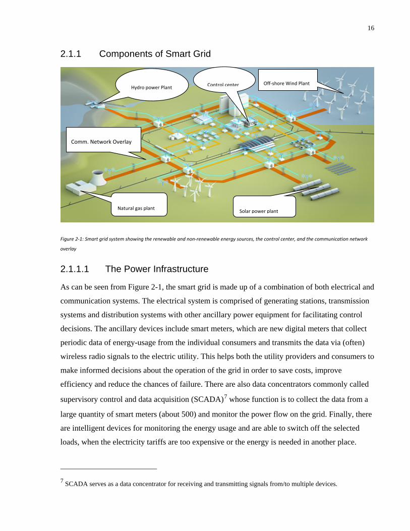
2.1.1 Components of Smart Grid

Figure 2-1: Smart grid system showing the renewable and non-renewable energy sources, the control center, and the communication network

overlay

2.1.1.1 The Power Infrastructure

As can be seen from Figure 2-1, the smart grid is made up of a combination of both electrical and

communication systems. The electrical system is comprised of generating stations, transmission

systems and distribution systems with other ancillary power equipment for facilitating control

decisions. The ancillary devices include smart meters, which are new digital meters that collect

periodic data of energy-usage from the individual consumers and transmits the data via (often)

wireless radio signals to the electric utility. This helps both the utility providers and consumers to

make informed decisions about the operation of the grid in order to save costs, improve

efficiency and reduce the chances of failure. There are also data concentrators commonly called

supervisory control and data acquisition (SCADA)7 whose function is to collect the data from a

large quantity of smart meters (about 500) and monitor the power flow on the grid. Finally, there

are intelligent devices for monitoring the energy usage and are able to switch off the selected

loads, when the electricity tariffs are too expensive or the energy is needed in another place.

7 SCADA serves as a data concentrator for receiving and transmitting signals from/to multiple devices.

Hydro power Plant Off-shore Wind Plant

Comm. Network Overlay

Natural gas plant Solar power plant

Control center

17

From the foregoing, it’s obvious that these devices need some means of communication

considering they are usually located some distance away from one another. And even when they

are close, they may not be operating on the same protocol. And that is the discussion of Section

2.1.1.2.

2.1.1.2 The Cyber Infrastructure

Overlaying the power infrastructure is the communication network which is responsible for the

smooth operation of the power grid by ensuring efficient data exchange amongst the various

devices and generators connected to the power grid. The communication could be realized via a

variety of media including radio, fiber optics, power line carriers, telecommunication cables or a

combination. The cyber infrastructure will ideally possess some features like plug and play

capability, possibilities for mapping to different physical layers, and expandability of the data

models and introduction of new models in accordance with the new and enhanced

communication tasks. In Figure 2-1, it demonstrates how a communication overlay can run

across the span of the power grid to provide communication and coordination amongst the DERs

in the power grid. This helps to make the smart grid a horizontally configured system. Hence, all

the DERs can participate in meeting the power demand on the grid and as well regulate the

frequency of the power system to ensure a stable operation. This capability enables engineers

and researchers to design a hierarchical control approach in which different levels of control can

be applied, hence, optimizing the operation of the system.

2.2 Smart Grid Co-Simulator

2.2.1 Types of co-simulator

A smart grid co-simulator is a software Integrator; that helps to simulate the practical smart grid

operation by enabling different federated simulators to run concurrently or serially, and in

coordination with each other to depict a desired scenario of the smart grid under study. This is

important as the two main components that form the smart grid have different simulation

modeling characteristics as we have highlighted in the introduction of the thesis. However, the

software Integrator is classified into two types based on whether it is real-time and off-line.

18

2.2.1.1 Real-time co-simulator

For decades, simulators played a major role in the design and planning of electrical power

systems. From aerospace studies, transmission line layout design, home electronics design to

optimization of the motor drives in transportation, simulation has helped us to imagine, plan,

design and implement our thoughts before implementing the ideas physically. However, the

rapid evolution of simulation tools, primarily due to decreasing cost of computing devices and

increasing capability of these devices to solve more complex problems with less time, greatly

provides a new vista in the simulation world. The reduced cost has equally made simulation tools

more accessible by a wide variety of audiences. According to [24], a simulation is the

representation of the operation or features of a system through the use or operation of another.

During real-time simulation, the accuracy of the computations not only depends upon precise

dynamic representation of the system, but also on the length of time used to produce results [24].

For a real-time simulation to be valid, the real-time simulator used must accurately produce the

internal variables and outputs of the simulation within the same length of time that its physical

counterpart would. In fact, the time required to compute the solution at a given time-step must be

shorter than the wall clock duration of the time-step. This permits the real-time simulator to

perform all operations necessary to make a real time simulation relevant, including driving inputs

and outputs (I/O) to and from externally connected devices.

For a given time-step, any idle-time preceding or following simulator operations is lost; as

opposed to accelerated simulation, where idle time is used to compute the equations at the next

time-step. In such a case, the simulator waits until the clock ticks to the next time-step. However,

if simulator operations are not at all achieved within the required fixed time-step, the real-time

simulation is considered erroneous. This is commonly known as an “overrun.” Based on these

basic definitions, it can be deduced that a real-time simulator is performing as expected if the

equations and the states of the simulated system are solved accurately, with an acceptable

resemblance to its physical counterpart, without the occurrence of overruns. Real-time digital

simulation is based on discrete time-steps where the simulator solves model equations

successively. Proper time-step duration must be determined to accurately represent the system

frequency response up to the fastest transient of interest. Simulation results can be validated

when the simulator achieves real-time without overruns. Basic functions performed in each time-

19

step include; read input and generate output, solve model equations, exchange results with other

simulation nodes, and wait for the start of the next step. Therefore, in real time co-simulator,

both the power and communication simulator have the capability of doing real time simulation.

This type of simulation helps us to understand two main issues:

• Whether the proposed design or algorithm in the simulation can be digitally implemented

in an industrial hardware platform.

• The effects of practical issues, including noise, non-idealities associated with analogue-

to-digital, sampling rate of digital controllers, which ordinarily would not manifest in off-

line simulation.

2.2.1.2 Off-line co-simulator

For digital simulation, it is assumed that a simulation with discrete-time and constant step

duration is performed. During discrete-time simulation, time moves forward in steps of equal

duration. This is commonly known as fixed time-step simulation [24]. It is important to note that

other numerical solving techniques exist that use variable time-steps. Such techniques are used

for solving high frequency dynamics and nonlinear systems because of its accuracy and ability to

solve algebraic loops. The advantages derived from using variable-step solvers are obtained on

the condition that the solvers take the required processing time to achieve the specified accuracy,

hence, the processing time cannot be easily controlled and varies for each time-step. This makes

variable-step solvers unsuitable for hard real-time simulation requiring to maintain a fixed

processing time. To solve mathematical functions and equations at a given time-step, each

variable or system state is solved successively as a function of variables and states at the end of

the proceeding time-step. During a discrete-time simulation, the amount of real time required to

compute all equations and functions representing a system during a given time-step may be

shorter or longer than the duration of the simulation time-step. This technique is implemented

using two methods: one in which the computing time is shorter than the fixed time-step (also

referred to as accelerated simulation) and one in which the computing time is longer. These two

situations are referred to as off-line simulation. In both cases, the moment at which a result

becomes available is irrelevant. Typically, when performing off-line simulation, the objective is

to obtain results as fast as possible. The system solving speed depends on available

computational power and the system’s mathematical model complexity.

20

2.2.2 Components of smart grid co-simulator

Figure 2-2: Diagram showing the interaction of the components of the smart grid co-simulator

2.2.2.1 Power Simulator

A smart grid consists of energy sources, transmission networks and distribution components, all

containing of both physical components and ICT. The power generators are comprised of a

combination of thermal power plants, hydro power plants, solar power plants, wind power plants,

biogas power plants, etc. The transmission system consists of the towers, underground or

overhead cables, and the substation step up or step down transformers, etc. And the distribution

system has the feeders, step down transformers, cables, insulators as well as some form of

distributed energy sources as its components. In modeling smart grid systems, these components

need to be captured in the simulation. Therefore, in our federation of simulators, we include a

simulator capable of handling all the power modeling, and simulation needs of the multi-domain

21

system with regard to the power system off-line simulation in time-domain. In our case, we

incorporate PSCAD/EMTDC, which is where the design and implementation of the physical

power components of the smart grid is done. It has a graphical user interface which makes

human interaction with the simulator easier, and enables the design, implementation and

visualization of the results of the simulation. EMTDC is the simulation engine of the simulator,

and it is responsible for translating the models designed in PSCAD into equations and carry out

the computation. Finally, results are transmitted back to PSCAD for visualization. The choice of

PSCAD/EMTDC is mainly because our interest is in transient simulation studies and

PSCAD/EMTDC is among the few power simulators with the capabilities to carry out such

simulation. It can solve power systems with time ranging from nanoseconds to seconds but our

interest is in the transient studies which falls under the milliseconds range.

2.2.2.2 Communication Simulator

Different distributed resources in smart grid are able to coordinate their actions in controlling the

grid frequency and meeting power demand need because of the communication network overlay

in the grid. Usually, communication networks of different protocols are used to regulate the

transmission of information in smart grid. It could include wireless, wired, power line

communication, etc., It could also be characterized as a high or low bandwidth network

depending on the specification of the system under study. Now, modeling and studying the

statistical nature of communication network requires a communication simulator incorporated

into the multi-domain simulation. Therefore, to solve this need, we include a communication

network into the multi-domain simulator so as to handle all the modeling, design and

implementation of communication networks in the smart grid. In Figure 2-2, the communication

simulator is OMNET++ and it is this simulator that makes the grid more intelligent. This is

because, a traditionally centralized grid can be converted to a distributed grid with multiple

control structures to enhance efficiency, scalability and security of the power system. The

communication simulator provides basic graphical interfaces like start, stop and pause. The

INET is a framework built above OMNeT++ that provides Internet specific support for both

wired and wireless communication simulations. The IED (Intelligent Energy devices) as well as

the network topology is built into the communication simulator using models derived from INET

framework.

22

2.2.2.3 Control Simulator

Managing a power system involves some decision-making. Some are very basic decisions that

involve using a digital or logical controller. Others are complex, requiring more flexible

computations. Because of the distributed nature of the smart grid, some rigorous energy

management systems are installed to regulate and control the numerous distributed energy

resources attached to the grid. This is necessary as all of the energy sources participate in

regulating the frequency of the grid, and meeting the energy demand on the grid. Hence, in our

co-simulation platform, we incorporate a computational software which is capable of handling

all the specialized control features which ordinary power or communication simulator cannot

handle. In smart grid, a hierarchical control architecture is a common feature in which the

highest level of control participates in power management optimization and sends reference

signals to lower level controllers that implement the decisions. Modeling this top level controller

requires flexible computational software such as MATLAB/Simulink. Therefore, in a bid to

make our co-simulator versatile, we include MATLAB/Simulink in our federation of simulators

to solve the control engineering related problems.

2.2.2.4 Scheduler

In our federation of simulators, the power simulator, the communication simulator and the

control engineering simulator have been identified, but how they work together to make the

simulation realizable requires another piece of software which we call a scheduler. This software

is responsible for regulating the interaction amongst the federating simulators by determining

when each of them runs, imports data from each of them, processes the data, stores the data when

necessary, and exports the data to any of the simulator that needs it. It is also in this software that

the configuration of the sensor rates of the power system measurement is done. It is independent

of any of the simulators and can be built in any language. However, we program the software in

C language and embed it into the federation. The scheduler has an open source database called

SQLite, which is used to provide short history for the system. Providing the history of the system

is necessary in our design in order to enable us to eliminate errors which usually occur in many

synchronization processes highlighted in the previous chapter. The choice of employing the C

language for programming the software is for ease of integration with the rest of the simulators

as each of them has Application Programmable Interface (API) that can interact with C/C++

source files.

23

2.2.3 Methods of co-simulation

When we carry out distributed simulation, there is typically a defined way for data exchange

amongst the various components. This can be categorized as interactive and non-interactive co-

simulation.

2.2.3.1 Interactive co-simulation

Otherwise known as full co-simulation, this is a type of co-simulation in which the federating

simulators dynamically exchange data amongst themselves as the simulation progresses. Here,

there is full to and fro movement of information among the simulators based on design

instructions. Hence, dynamic activities in the systems involved in the federation can be modelled

and captured in the simulation [9].

2.2.3.2 Non-interactive co-simulation

As the name suggests, this type of simulation captures only dynamic activities in one of the

simulators while the other simulator is modelled as a static system. Usually, the data in the

simulator, which models the static system is extracted and stored before the dynamic simulator is

run. The data is then applied to the simulator, which models the dynamic system as the

simulation progresses according to the design instructions. Example of this scenario is a co-

simulation involving a communication network and power system in which delay values are

extracted from the communication simulator, saved and applied to the power simulator by hard

coding the values or using buffer files and the power simulator picks the delay values as the

simulation progresses. Here, disruptions, failures, etc., in the power system model can easily be

captured, but that is not the case with the communication network model which maps the power

system under study.

2.3 Smart grid co-simulator modeling approaches In order to carry out studies on smart grid, we first need to develop a model, solve or implement

the model and check whether we have an acceptable result depending on our interest of study. In

doing this, so many approaches are adopted in developing the co-simulator that will help us solve

the smart grid problem. Some of the methods are used alone, and some in conjunction with one

another. But the two major approaches adopted in developing a co-simulator are: mathematical

models and empirical models.

24

2.3.1 Mathematical models

The general procedure for predicting the behavior of a system is modeling. In this method, we

build models that predict a system's behavior. A model of a system represents a surrogate whose

behavior mimics that of the system. Models are classified into two: physically built and

mathematical [25]. One of the most commonly used models today is a mathematical model, since

they are the most adaptable and inexpensive. In specific applications, mathematical models

consist of computer codes that are easily modified to accommodate fluctuations in system

properties. Mathematical models are a blend of scientific and technological knowledge with the

aim of predicting system performance. Such knowledge is, thereby, incorporated into the

computational codes that the computers execute in model applications. At present, mathematical

models founded on numerical simulation make it easy to study complex systems and natural

phenomena that otherwise would be very expensive, harmful, or even impossible to study by

direct experimentation [25]. From this perspective the significance of mathematical and

computational modeling is clear as it presents the most efficient and effective means of

predicting the behavior of both natural and artificial systems of human interest. This approach is

adopted in studying complex systems like weather, power systems and even used in the oil and

gas industry. Mathematical models are made up of relationships and variables. Relationships can

be described by operators, such as algebraic operators, functions, differential operators, etc.,

while variables are abstractions of system parameters of interest, which can be quantified.

Mathematical models can be classified in the following ways:

2.3.1.1 Linear and nonlinear models

A system is said to be linear if the mathematical model of the system is based on the use of a

linear operator. Hence, if all the operators in a mathematical model exhibit linearity, the resulting

mathematical model is defined as linear. A model is considered to be nonlinear otherwise. The

definition of linearity and nonlinearity is dependent on context, and linear models may have

nonlinear expressions in them. For example, in a statistical, linear model, it is assumed that a

relationship is linear in the parameters, but it may be nonlinear in the predictor variables.

Similarly, a differential equation is said to be linear if it can be written with linear differential

operators, but it can still have nonlinear expressions in it. In a mathematical programming model,

if the objective functions and constraints are represented entirely by linear equations, then the

25

model is regarded as a linear model. And if one or more of the objective functions or constraints

are represented by a nonlinear equation, then the model is known as a nonlinear model [26].

The presence of nonlinearity in system model always complicates the study of the system and

makes it more difficult to study than linear systems. Usually, the principle of linearization is used

to simplify the system and solve it using linear methods. Although, it should be noted that

linearization does not hold the solution to every nonlinear model, especially the ones related to

irreversibility.

2.3.1.2 Static and dynamic models

This is also called steady state (static) and dynamic system. While dynamic model accounts for

time-dependent changes in the state of the system, a static model calculates the system in

equilibrium, and thus is time-invariant. Common representation of dynamic models is via

differential equations. These kind of models are used to model system stability, system

optimization, etc.

2.3.1.3 Deterministic and stochastic models

In a deterministic model, every set of variable states is uniquely determined by the parameters in

the model and by sets of previous states of these variables; therefore, the output of the model is

always consistent given a set of initial conditions. Conversely, in a stochastic model, randomness

is always present, and variable states are not described by unique values, but rather by

probability distributions [27]. In summary, given initial conditions, output of deterministic model

can be predicted with a high degree of accuracy, but that is difficult for the stochastic model.

Example of a stochastic process is the delay experienced in a communication network while

Newton’s law of physics is a case of deterministic systems.

2.3.1.4 Discrete and continuous models

A discrete model treats objects as isolated sets, such as the particles in a molecular model or the

states in a statistical model; while a continuous model represents the objects in a continuum of

possible states, such as the velocity field of fluid in pipe flows, temperatures and stresses in a

solid, and electric field that applies continuously over the entire model due to a point charge.

Discrete models represent an instant in time when an event occurs; in between events, the state

26

of the system is assumed constant. Whereas in continuous models, the events are from a

continuum and thus are dependent.

2.3.2 Simulation modeling

A simulation is an applied methodology that can describe the behavior of a system using either a

mathematical model or a symbolic model. It is also defined as the imitation of the operation of a

real-world process or system over a period of time [28]. When the real system cannot be

involved, simulation becomes the obvious choice. And the real system may not be involved

because of the following reasons:

• It may not be accessible,

• It may be dangerous to engage the system,

• It may be unacceptable to engage the system, or

• The system may simply not exist.

So to counter these objections, a computer will "imitate" operations of these various real-world

facilities or processes. In the field of distributed or federated simulation, two major types of

simulation are identified: interactive and non-interactive co-simulation.

2.3.2.1 Interactive simulation

Interactive simulation is a special kind of physical simulation, often referred to as a human in the

loop simulation, in which physical simulations include human operators, such as in a flight

simulator or a driving simulator. However, if human operators are replaced by another simulator,

the system is termed a distributed simulation or a co-simulation. Here, the dynamics inside any

of the simulators is shared amongst the federating simulators according to a defined data

exchange policy during the course of the simulation. This could be real-time or off-line, but the

most important feature is that each simulator reacts to both its own dynamics and that of other

federating simulators. Hence, there is a bi-directional flow of information during the simulation.

This is illustrated in Figure 2-3 below.

27

Figure 2-3: Interactive co-simulation depicting the bi-directional information exchange.

2.3.2.2 Non-interactive simulation

When there is only one direction of information flow, the co-simulation is said to be non-

interactive. Under this condition, simulator A transfers data to simulator B when it needs it, but

the converse is not true. Hence, while the output of simulator B is a product of its own dynamics

and that of the external simulator, the output of simulator A entirely depends on its own

dynamics. Figure 2-4 demonstrates this type of relationship.

Figure 2-4: Non-interactive co-simulation showing unidirectional flow of information.

2.4 Synchronization in smart grid co-simulation When more than one simulator is involved in a simulation, a problem of synchronizing the

simulation time of the simulators arises. This is necessary as we model practical scenarios in

which we cannot process an event in which its time has passed nor can we process an event in

which its time has not reached as this would result in incorrect modeling of the scenarios

involved or binging the simulators to an unexpected halt. Therefore, the challenge in using off-

line simulator is to process each event at exactly the timestamp it bears. When real-time

simulators are used, this challenge is integrally taken care of as the simulation time is same as

wall clock time. Hence, no need for synchronization. However, off-line simulators offer more

scalability than real-time simulators. Hence, the need for a rigorous process of synchronizing the

28

simulation time of the simulators. To solve this problem, many ideas are canvassed as

enumerated in the Table 2-1 below.

Table 2-1 Synchronization methods in some reviewed works.

Components Synchronization

EPOCHS[9] PSCAD, PSLF, NS2 Periodic

ADEVS[16] Adevs,NS2 Event-based

[20] Simulink, OPNET Not addressed

VPNET[6] Virtual Test Bed, OPNET Periodic

PowerNet [14] Modelica, NS2 Periodic

[21] OPNET only, Virtual Power System Delay estimation

SCADA CST [29] PowerWorld, RINSE Non-interactive

TASSCS [30] PowerWorld, OPNET Non-interactive

GECO [7] PSLF, NS2 Event-based

As can be seen from Table 2-1, the synchronization method can broadly be classified into two

types: periodic and event-based synchronization.

2.4.1 Periodic Synchronization

A situation in which there is an explicit synchronization time defined before the simulation starts

is called periodic synchronization. Here, the federated simulators are allowed to run

simultaneously, and periodically communicates with one another at every synchronization step.

Usually, a run time infrastructure which acts as a coordinator is embedded into the federation to

coordinate this data exchange and ensure that the simulation time of each of the simulators is

synchronized with the global synchronization time [9].

29

2.4.2 Event-based Synchronization

In some cases, there is no explicit defined synchronization point and the simulation time of the

simulators must not be synchronized to any reference. Rather, an event queue is developed which

stores events according to their timestamps. Here, the queue is made up of events from different

simulators and a scheduler determines when each event is processed and by which simulator.

This way, the simulators take time to run according to which event is next on the queue. This has

so many advantages as it eliminates accumulated errors inherent in periodic synchronization and

also removes the expensive process of building a runtime infrastructure that synchronies the

simulation time of each of the simulators involved in the simulation. Reference [7] uses this

method and it proved very effective in eliminating the most demerits of the periodic

synchronization experienced in [9].

2.5 Data Exchange in Smart Grid Simulation In distributed computing, simulation, system integration, etc., the communicating devices usually

have a means of getting access to data held by other devices in the federation. This could be in

the form of file system access, shared memory, windows pipes or sockets, etc. In our model for

instance, the devices in PSCAD/EMTDC will generate data that would be passed to OMNET++

or MATLAB/Simulink for processing. And when these simulators are done with processing of

the data, a set of command or control instructions are sent back to the devices in

PSCAD/EMTDC for necessary action. This task can be accomplished in many ways, but

prominent among them is the method used by [9] in which a Runtime Infrastructure is built to

manage the data exchange between different simulators involved in the simulation. Also, Globe

Scheduler is implemented by [7] by creating a discrete time-event based schedule that uses

timestamps to sort the events and processes them accordingly. While these methods are efficient,

their efficiency is low [4]. To increase the efficiency of this process, it would be better to employ

the use of Inter-Process Communication (IPC) to manage data exchange between these

simulators as it has been the default way of making stand-alone process communicate with one

another. It is fast, it is efficient and it can support real time transmission. Next, we discuss

different implementations of IPC. It simplifies the division of labor among processes, simulators

or computers in a network.

30

2.5.1 Pipes

In computer networking, a pipe is conceived of as an information conduit. It is assumed to have

two ends-one where the information is read, and one where information is written to. It is also

called a special FIFO8 file because of how it saves information in memory. It could also be

simplex or bi-directional. When it is a simplex pipe, only one end allows reading of data while

the other end allows writing of data. On the other hand, a bi-directional pipe allows reading and

writing of data from both ends. Two major classifications of pipes are: anonymous pipe and

named pipe [31].

• Anonymous pipe: A traditional Unix-like pipe that is used for transfer of information

from parent to child processes. Hence, it is only process persistent and dies when the

process dies and is not used for communication across a network. Also, it is a simplex

pipe, i.e. it only allows a unidirectional flow of information.

• Named pipe: It could be simplex or duplex and is used for communication between a pipe

server and client(s). It is system persistent and can be used for communication over the

network and locally. The term pipe server refers to the creator of the named pipe and pipe

client refers to processes that connect to the instance of the named server. In order to

allow multiple clients to use the named pipes simultaneously, instances of the named

pipes are created which share the same name, but have different buffers and handles,

which are used to provide communication between client/server separately.

2.5.2 Shared Memory

This uses a file mapping scheme which allows multiple processes to see the contents of a file as

if they were a block of memory in the process's address space. To accomplish this, each process

that wishes to access the same file mapping is given a pointer to memory in its own address

space which can be used to access the contents of the file. And to avoid concurrent access to the

file by multiple processes, a file locking system like semaphore is always implemented which

provides synchronization and prevents data corruption. In order to make the file mapping file to

8 FIFO is a special access technique which ensures First In, First Out for data in memory.

31

be seen as a shared memory block, a system swapping file is named during the file-mapping

object creation. This enables other processes to access the same block of memory by opening

same file-mapping object. While this is an efficient IPC scheme, its scope is limited only to a

local computer and cannot be used over the network.

2.5.3 Sockets

A protocol independent interface that is used both in windows and UNIX based systems.

Although the implementation details for each case is different, the underlying principle is the

same as both make use of the communication capabilities of the underlying protocols. A socket

is one endpoint of a two-way communication link between two programs running on the

network. A socket is bound to a port number so that the TCP layer can identify the application

which is the data sink. This process usually involves one or more clients and a server. The

development of most socket Application Programmable Interfaces (APIs) is based on the

standard popularized by Berkeley Software Distribution (BSD). It has become the most popular

means of inter-process communication, especially in a large networked system because of its

flexibility and efficiency. It handles both local and over the network communication efficiently

and this is the scheme we implement in our work.

2.6 Tool Sets Discussion In a distributed simulation, more than one simulator is usually involved in accomplishing the

task. In our own case, we federate three simulators with the PSCAD/EMTDC serving as a power

simulator, the OMNeT++ serving as a communication simulator, and the MATLAB/Simulink to

be used as a control engineering simulator. Below is a brief description of each.

2.6.1 PSCAD/EMTDC

PSCAD is the graphical user interface to the simulation engine called EMTDC. EMTDC is

developed to handle electromagnetic transient simulation, hence can capture dynamics in the

power systems from microseconds to seconds. PSCAD being the graphical interface, is where

the schematic construction of a circuit, running of a simulation, analysis of results and exporting

of the data to third party software for further processing is handled. It has online plotting

functions as well as meters and controls which could be used to modify the simulation

constraints during the run and observe the effects of such changes. The simulator has a pre-

32

programmed and tested simulation models, comprising of simple control functions, passive

elements like resistors, as well as complicated models like transmission lines and cables. To

extend the flexibility of using the simulator, it allows users the freedom to build their own

models in either FORTRAN or C programming language and incorporate it in the model. And it

is this capability that we will utilize in the development of our federated simulator. The choice of

PSCAD is based on its capability to capture transient dynamics which is our target area.

2.6.2 OMNeT++ /INET

OMNeT++ is an object-oriented, discrete event simulation framework. Its modular architecture

has been exploited in developing and simulating models in various disciplines outside

communication engineering. Some of the areas in which it has been used includes but not limited

to validating hardware architecture, protocol modeling, wired and wireless network

communication modeling, and other general modeling and simulation architectures that are

modular and discrete event driven. OMNeT++ provides the infrastructure for writing the

simulation, but not a simulator on its own. It only provides reusable modules which are

hierarchically designed for the user to assemble as desired to facilitate the simulation. INET

framework is an example of one of the reusable modules that is specifically designed for TCP/IP

and UDP simulation in OMNeT++ and serves as the underlying framework in our models.

2.6.3 MATLAB/Simulink

MATLAB is a high-level language that handles visualization, programming and numerical

computation. It is used to develop algorithms, create applications, do data analysis, etc. It has in

built functions and numerous tools that aid in designing models, running simulations and

implementing wide range of ideas in many disciplines such as communication and signal

processing, control engineering, finance, image and video processing, etc. MATLAB equally has

a rich Application Programmable Interface for integrating models developed in other languages

like C/C++ or Java, and this flexibility has made MATLAB one of the most popular

computational software. In our case, it is used in the energy management system to optimize the

set point of the distributed generators.

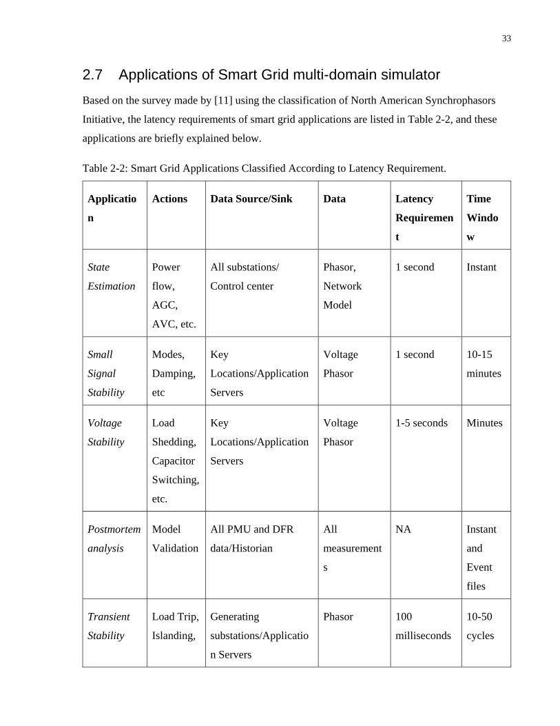
33

2.7 Applications of Smart Grid multi-domain simulator Based on the survey made by [11] using the classification of North American Synchrophasors

Initiative, the latency requirements of smart grid applications are listed in Table 2-2, and these

applications are briefly explained below.

Table 2-2: Smart Grid Applications Classified According to Latency Requirement.

Applicatio

n

Actions Data Source/Sink Data Latency

Requiremen

t

Time

Windo

w

State

Estimation

Power

flow,

AGC,

AVC, etc.

All substations/

Control center

Phasor,

Network

Model

1 second Instant

Small

Signal

Stability

Modes,

Damping,

etc

Key

Locations/Application

Servers

Voltage

Phasor

1 second 10-15

minutes

Voltage

Stability

Load

Shedding,

Capacitor

Switching,

etc.

Key

Locations/Application

Servers

Voltage

Phasor

1-5 seconds Minutes

Postmortem

analysis

Model

Validation

All PMU and DFR

data/Historian

All

measurement

s

NA Instant

and

Event

files

Transient

Stability

Load Trip,

Islanding,

Generating

substations/Applicatio

n Servers

Phasor 100

milliseconds

10-50

cycles

34

Generatio

n Trip

2.7.1 State Estimation

This provides an internal state of the given power system using measurements from the PMUs. It

tries to minimize the effects of corrupt or bad data on the computation of the system state.

2.7.2 Small Signal Stability

The ability of the power system to maintain synchronism when subjected to small disturbance

refers to small signal stability. It’s an event that occurs over time and collecting signals from key

locations, and observing mode damping, preventive measures can be taken to forestall the small

signal instability.

2.7.3 Voltage Stability Analysis

Deficiency in reactive power in an area can easily cascade and lead to system failure. Therefore,

voltage stability studies tries minimize the occurrence of this by taking voltage measurement in

an area and using VAR balancing or Islanding as a stabilizing measure. The distance that usually

exists between the source of the measured data and where it is processed implies that an effective

and reliable communication system is vital in this study. Therefore, this forms a core part of

smart grid applications that should benefit from multi-domain simulators like the one proposed

in this thesis.

2.7.4 Postmortem Analysis

Latency requirement is not applicable to this application, and it uses PMU data as well as data

from digital fault recorders (DFR) to update the engineering setting of the system.

2.7.5 Transient Analysis

This relates to the speed and internal angles of the generators in a power system but for

microgrid that is not using synchronous machines, it refers to the behavior of the system when it

is subjected to heavy transient disturbances such as loss of large loads or loss of generation. The

35

latency is small and the system requires fast control scheme in order to prevent it from becoming

transiently unstable.

2.8 Summary In this chapter, we described various aspects of smart grid co-simulation ranging from its

individual components to a variety of classifications. We provided a detailed discussion of

several modeling approaches in smart grid co-simulation. Then, the synchronization techniques

that have been used in smart grid studies were discussed as well as the data exchange options

that are most prevalent. Finally, we discussed the tool sets used in this work as well, and

provided the classification of smart grid application based on latency requirements. The table

below provides the key points of the two simulation methods.

Table 2-3: Smart grid co-simulation approaches with the pros and cons of each method

Simulation approaches Merits Demerits

Real-time co-simulation 1. No synchronization

required.

2. Could be faster for

systems with less

switching and non-

idealities.

1. Does not solve

algebraic loops.

2. Uses fixed time-steps,

hence knowledge of

appropriate time-step

is required.

Off-line co-simulation 1. Uses variable-step to

speed up the

simulation.

2. Better accuracy.

3. Solves algebraic

loops.

4. Higher numerical

stability.

1. Tolerance range and

type of solver must be

provided.

2. Synchronization is

required.

3. Uses fixed time-steps

for some systems.

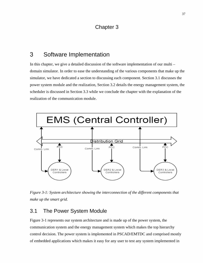
37

Chapter 3

Software Implementation In this chapter, we give a detailed discussion of the software implementation of our multi –

domain simulator. In order to ease the understanding of the various components that make up the

simulator, we have dedicated a section to discussing each component. Section 3.1 discusses the

power system module and the realization, Section 3.2 details the energy management system, the

scheduler is discussed in Section 3.3 while we conclude the chapter with the explanation of the

realization of the communication module.

Figure 3-1: System architecture showing the interconnection of the different components that

make up the smart grid.

3.1 The Power System Module Figure 3-1 represents our system architecture and is made up of the power system, the

communication system and the energy management system which makes the top hierarchy

control decision. The power system is implemented in PSCAD/EMTDC and comprised mostly

of embedded applications which makes it easy for any user to test any system implemented in

38

PSCAD/EMTDC in the co-simulator with minimal work. In Figure 3-1, DERs, the distribution

grid and the connecting lines make up the power system module. Below is the figure which

describes the software architecture of the whole system.

Figure 3-2: Software Architecture of the Co-simulator with all the key components

We implement a system that could function like a plug and play device. So the role of each block

is explained below.

3.1.1 Power System Design in PSCAD

As described in previous sections, PSCAD is the graphical user interface for the EMTDC

simulation engine and this is where each user of the co-simulator can design any conceived

power system. With our software, our idea is that each person that wants to use the co-simulator

can design his/her own power system in PSCAD and use it in our system for transient studies in

the time domain that involves co-simulation without doing much work in modifying our system.

Hence, the type and scale of what is obtainable in this platform is only a decision made by the

39

user of the system. The pre-programmed models in PSCAD as well as the user defined models

can be used in this section for designing the desired system. Also, PSCAD is rich with many

control and input functions which are used to adjust the parameters of the system as the

simulation is running. PSCAD became a natural choice for us because it can simulate short

transient disturbances with high fidelity, and that is our area of interest. Finally, the results can

be analyzed in the PSCAD using various plotting tools or could be exported to third party

software like excel for further analysis and processing.

3.1.2 EMTDC and C Interface

EMTDC is the simulation engine of the PSCAD software and one vital feature of the software

which we exploit in the development of the multi-domain simulator is the freedom to build a

custom model and embed it into the simulation engine. FORTRAN source code, C source or

object files can be incorporated into the simulation engine using a special Application

Programmable Interface (API) provided by Manitoba Hydro who are the licensed owners of the

software. Therefore, pre-programmed models which are not in the supplied library that ships

with the software can be built using any of the mentioned programming languages above. With

this extension capability, we designed an interface using the C programming language to enable

the EMTDC to import and export data from the scheduler. For internal interactions (between

PSCAD and EMTDC custom built models), we develop a C subroutine which eases interaction

between the custom built models and the pre-programmed models in PSCAD. For external

interactions (between PSCAD/EMTDC and scheduler), we employ inter-process communication

using windows sockets programmed using the C programming language. The choice of windows

socket is obvious as we wanted something that is protocol independent and faster. And the ability

of the socket communication to make use of underlying operating system communication

capabilities has been proven to speed up communication based on the socket networking

communication. This interface contains two essential parameters which ought to be manually

configured by the user of the software and below is a description of both;

• Dynamic Buffer: A key design parameter and determines the quantity of data that could

be transferred out of and into EMTDC. To make the software scalable, we settled for a

dynamic buffer so that the volume of data that could be exchanged between EMTDC and

the rest of the system is only constrained by the available hardware storage in the

40

computer systems used in the simulation. This could be likened to statistical multiplexing

technique and allows freeing of the communication buffers and bandwidth for other

forms of traffic when the smart grid traffic is small in size. As expected, this feature is

present for both inbound and outbound traffics on both the EMS and the power simulator.

All that is required to activate the dynamic buffer is the knowledge of the number of

sensors that will be taking measurements in the system. This value would have to be

supplied by the user in the configuration file manually. The pseudo code for both the

outbound and inbound traffic are provided below.

Figure 3-3: Pseudo code for the dynamic buffer managing traffic from different sources going

into the communication network.

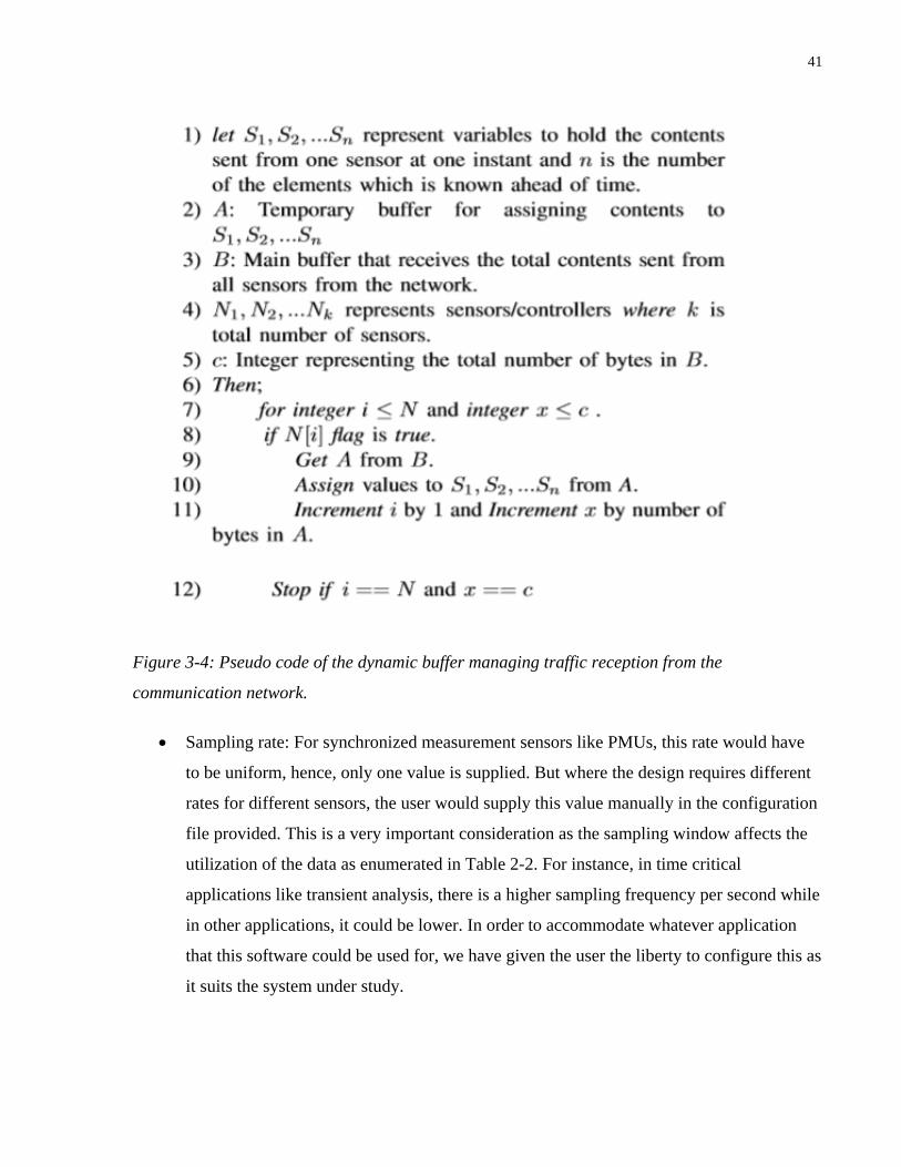
41

Figure 3-4: Pseudo code of the dynamic buffer managing traffic reception from the

communication network.

• Sampling rate: For synchronized measurement sensors like PMUs, this rate would have

to be uniform, hence, only one value is supplied. But where the design requires different

rates for different sensors, the user would supply this value manually in the configuration

file provided. This is a very important consideration as the sampling window affects the

utilization of the data as enumerated in Table 2-2. For instance, in time critical

applications like transient analysis, there is a higher sampling frequency per second while

in other applications, it could be lower. In order to accommodate whatever application

that this software could be used for, we have given the user the liberty to configure this as

it suits the system under study.

42

3.2 Energy Management System (EMS) In Figure 3-1, the EMS is the central controller. Again, this feature is incorporated in view of

different control and management structures available in smart grid. Generally, there are two

kinds of control systems structure: centralized and distributed control systems.

• Centralized control system: When the action performed by lower level controllers are

dictated by the information obtained from the central controller, then this arrangement is

called a centralized control system. Here, the central controller can instruct the lower

level controllers directly or if the system is so complex, a kind of hierarchy could be

created in which there are other controllers in between the top level and lower level

controllers. The communication between the top and lower level could be bidirectional

(feedback) or unidirectional (open loop) as the case may be but the lower level controllers

will always depend on instructions from the central controller.

• Distributed control system: As the name suggests, when the lower level controllers

function based on local information only, then the system is said to be a distributed or a

decentralized system. The major difference here is that the lower level controllers make

their decisions without depending on the instructions of any commanding influence.

Therefore, we integrate the EMS into our work so that any study system that requires a

centralized or hierarchical control system could easily be studied without many changes to the

underlying software. The system can equally handle a system that has a purely decentralized

control system. In order to accommodate both behaviors without degrading the results of an

experiment, we give the user the option of enabling or disabling the EMS during the simulation

configuration. And to ensure versatility in the control functions, we use the MATLAB/Simulink

computational software as the control/management system simulator. The choice of this is an

easy one considering the different field of study in which the software readily has the toolbox.

So, all that is required of the user is to design the control system in MATLAB/Simulink and the

rest of the system will be interacting with it as the need arises via the MATLAB/Simulink API

which is available in numerous programming languages. This way, data is fed into the

control/management system in MATLAB/Simulink and it returns the result to the sending

software after processing.

43

However, if the control system is a decentralized one and does not require heavy computational

decisions, then the EMS can be disabled, and the control and logical functions and tools inside

the power simulator is then utilized to design the controllers.

3.3 Scheduler As the name suggests, this is not a simulator, but a software component that is responsible for

coordinating the behavior of the simulators involved in the multi-domain simulation. It creates

the discrete-event queue of all events generated from the different simulators and sorts them

according to their timestamp, and then alternates the run of each simulator based on the next

event in the queue. The details of how this software is realized is explained in the sub-sections

below and the Figure 3-5 is the flowchart diagram of the interactions between different modules

in the software. It is worth mentioning that the choice of the simulator where this program is

embedded determines which programming language is used to implement it. In our case, we

embed it in the PSCAD/EMTDC simulator and because it allows only C or FORTRAN files, we

implement it using the C programming language.

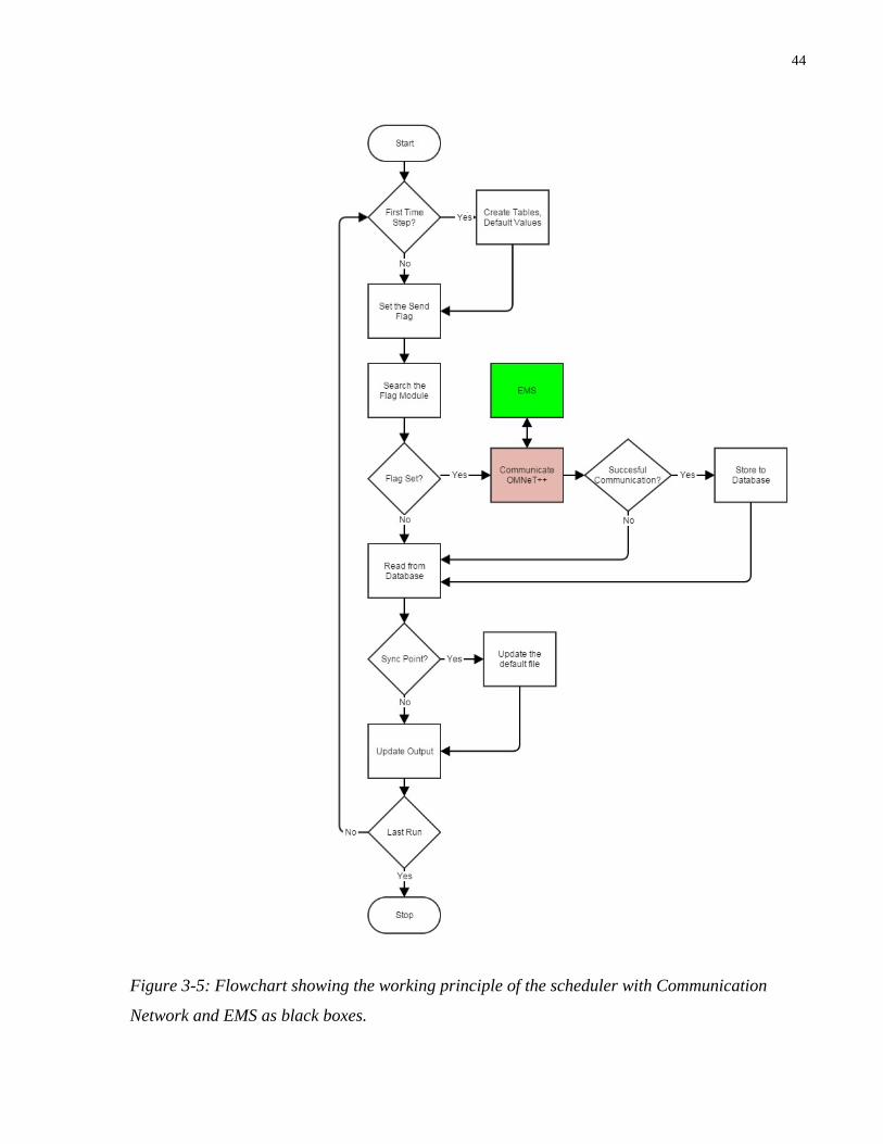
44

Figure 3-5: Flowchart showing the working principle of the scheduler with Communication

Network and EMS as black boxes.

45

3.3.1 Create Table Module ()

As shown in the flowchart, when the simulation starts, as part of the initialization process, the

scheduler checks to see if that is the first time-step of the simulation and if so, it creates the

database tables that will be storing the history for each of the physical sensor devices in the

power system. Checking whether it is the first time-step was necessary to ensure conflict free

table creation process and prevents the simulation from coming to a halt.

3.3.2 Create Default Status ()

After the successful creation of the tables, then the scheduler creates default values to be applied

to the physical devices in the power system and choosing what this value should be is a matter of

knowledge of the nature of the physical devices and their expected input values. The import of

this is to enable PSCAD/EMTDC progress with the simulation at the initial stage. This is as a

result of the simulator being a single threaded program and requires all declared variables to

have a value before the next step of the simulation is executed.

3.3.3 Rate Module ()

In order to take measurements from the physical devices in the power system and transfer them

to the control center via the communication channels, the scheduler incorporates a rate module

which is responsible for figuring out when values from each physical device should be sent to the

equivalent control center device for processing. If PMUs are used as the sensing device, then

there is a synchronized rate for the devices and the dynamic buffer manages how the data from

each device is arranged in the buffer and transmitted. If rather the rates are not the same and

there is no need for synchronization, then rate module, using the rates supplied by the user of the

software for each physical sensing device, decides when the measurements are taken.

3.3.4 Search Send Flag Module ()

When any physical device needs to communicate with the control center, it sets a flag. So, the

search send flag module is responsible for continuously scanning the send flag to see whether

any of the physical devices in the power system needs to communicate with the control center. If

no flag is set, the simulation proceeds. However, if a flag is set, then the scheduler queues it in

the event list and initiates the communication with OMNeT++ using the windows socket

communication, which in turn will hand over the simulation time to the communication and

46

control simulators. Because the simulators are single threaded simulators, this will automatically

pause PSCAD/EMTDC until the scheduler has a power event in the queue that it wants to

execute.

3.3.5 Socket Module ()

An essential component of the scheduler, it facilitates the data exchange amongst the three

simulators. We make this a socket client, which binds to the socket server in the communication

simulator and transfers data to and fro from the communication simulator when the need arises.

The choice of windows socket was primarily due to its efficiency, protocol independency, and

ability to network multiple computers running these simulators with ease. This function is

activated by the search send flag module if there is any physical device that has set a flag for

transmission. It should be emphasized that there is no delay between setting the flag and

transmitting the measurement because the events are sorted according to the timestamps of their

occurrence in the queue and executed accordingly.

3.3.6 Write Database Module ()

If the socket module was activated and the communication was successful, then the next thing the

scheduler does is to store the returned control values from OMNET++ in the database of the

system which is built using the small, light, open source database called SQLite. One of the

benefits of using the SQLite database is the ease of embedding it in any application because of

its small size. Also, it has API for most popular programming languages and we make use of the

C API of the database to store the timestamp and the returned control value in the database.

These saved values are used to create an event queue and are sorted for execution according to

their timestamp. The control values could represent reference set points from top level

controllers to lower level controllers or simple close or open command from the actuators to

circuit breakers.

3.3.7 Read Database Module ()

Because the event list is in the database, for every time-step during the simulation, the read

database module checks the database to find out if there is any physical device that needs its

status updated by passing an instruction in the queue to it. Which device status gets updated is

solely dependent on the time stamp which was used to sort the events. Hence, if multiple devices

47

share same time stamp, they all get updated at the same time. This process is cardinal in

eliminating accumulated errors which occur by explicitly fixing when the synchronization should

occur, which is otherwise called periodic synchronization.

3.3.8 Update Output Module ()

Like we stated earlier, the PSCAD/EMTDC simulator requires that every variable has a value

before it proceeds to the next step. Hence, after reading the database and checking for

synchronization point, the output status module is updated. And then the update output module

updates the status of the physical devices connected to the scheduler and the simulation

proceeds. Output status module is an intermediate module which ensures that if there is no

synchronization point, values in the previous history of the output status module are applied to

the devices, and this corresponds to a scenario in which the system dynamics is assumed not to

have changed over time. This is just to ensure that devices (represented as variables) always have

values during the simulation and prevents the simulation from coming to a premature halt.

3.4 The Communication System For the energy management system at the control center and the local controllers to

communicate, a communication link has to exist to link the systems together and it is the

incorporation of this feature that is shaping the development of smart grid. To this end, features

which hitherto are not obtainable in the traditional power system as a result of limitation of

hardware or lack of communication between different parts of the power system are now being

studied and integrated. With the inclusion of communication overlay in the power system, the

power system is more responsive and dynamic to consumer behavior. Also, it is now possible for

so many decentralized controllers of power plants to participate in maintaining grid frequency

and voltage via efficient coordination engineered by the use of communication network

infrastructure as against the old situation of using one large power plant to manage voltage

and/or frequency. To facilitate the understanding of how we realize our communication system

for the smart grid, we break it into the sub-sections below.

48

3.4.1 OMNeT++

From Figure 3-2, the top of the communication system software is the OMNeT++ framework.

This is a collection of reusable objected-oriented modules that can be assembled to do network

simulation. The modules are hierarchically designed and ranges from simple to compound

modules. Also, the OMNeT++ comes with eclipse-like Integrated Development Environment

(IDE) which allows for design, simulation and analysis of the study system conveniently using

the rich graphical interface. For those that like UNIX-like command line method, it also allows

simulation using the command line. It is built using the C++ programming language and it is an

open source software. On its own, OMNeT++ is not a simulator, it is a collection of C++ objects

which have been arranged as modules and these modules can be run on any system that has a

C++ compiler installed on it. The graphical interface has functions like run, stop, debug, etc., and

equally has some simple online plotting tools to analyze results. In our model, this is where the

mapping of the power system into its equivalent communication system is done. Mapped

modules represent the physical devices in the power system like fuse, switch, substation, etc.

Also, the distance between physical devices are represented using channels in the

communication system. And the channel connection of the physical devices could be wired using

fiber or coaxial cables or it could be wireless using Wireless Local Area Network (WLAN),

Metropolitan Area Network (MAN), etc. In order to mimic the behavior of communication

network, the modules exchange information in a discrete manner.

3.4.2 INET Framework

Being an open-source software, the community of developers that use the OMNeT++ software

have been using the modules found in OMNeT++ to deepen special areas of network and related

simulation, and one of the areas that has received great attention is the Internet Protocol (IP)

communication. The IP suite is the set of computer networking models used on the Internet. To

this end, the INET framework for OMNeT++ has been evolving over time and solely serve as an

underlying framework for IP suite communication in the OMNeT++ simulation of systems that

use the packet switching protocol. Packet switching transmission can be classified into

Transmission Control Protocol/IP (TCP/IP) and User Datagram Packet (UDP). Below is a

description of each:

49

3.4.2.1 TCP/IP

A type of packet switched protocol that uses acknowledgement to ensure a reliable byte stream

transfer. If there is packet drop or non-delivery, a lack of acknowledgement will signal a

retransmit of the packet unless the number of retries is exceeded, which will force the sender to

return a transmission failure message. This type of protocol is employed in applications which

emphasizes reliability. It has the characteristics of client-server communication with sender

representing client9 and server10 representing receiver. TCP/IP is a connection-oriented protocol

and uses a virtual circuit connection method. Therefore, the resource is secured when it is

required and released after it is used. The connection process is made up of three phases

described below and shown in Figure 3-7:

9 Client is the computer that sends a connection request. The client has to know the IP address of the server and the port number in order to send the request for connection. 10 Server is the computer device which bind to a port to create a passive open connection and wait for connection requests from clients. When the clients establishes the connection, it becomes an active open connection.

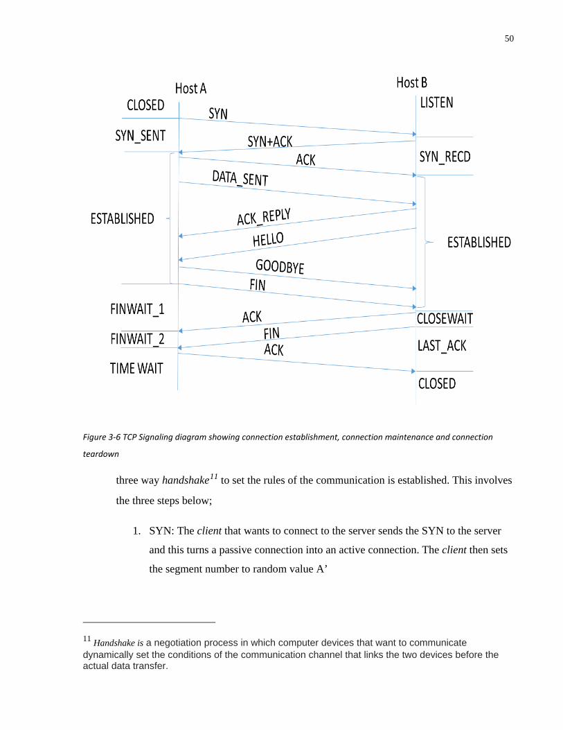
50

1. Connection establishment: In order to create a connection between a client and a server, a

three way handshake11 to set the rules of the communication is established. This involves

the three steps below;

1. SYN: The client that wants to connect to the server sends the SYN to the server

and this turns a passive connection into an active connection. The client then sets

the segment number to random value A’

11 Handshake is a negotiation process in which computer devices that want to communicate dynamically set the conditions of the communication channel that links the two devices before the actual data transfer.

Figure 3-6 TCP Signaling diagram showing connection establishment, connection maintenance and connection

teardown

51

2. SYN-ACK: In reply to the client request, the server sends the SYN-ACK message

with SYN number incremented by 1 (i.e. A+1) and another random value chosen

by the server to serve as the packet sequence number.

3. ACK: In the last lap, the client sends an ACK to the server with the

acknowledgement number retained as A+1 but the sequence number modified to

B+1. In this state the connection is established and the next phase begins.

2. Connection maintenance: After the step one above, a full duplex communication is

established using the sequence numbers and the two devices can start transmitting and

receiving data to and from each other.

3. Connection teardown: Similar to the connection establishment, this uses a four way

handshake and the steps are outlined below and are shown in Figure 3-7.

1. FIN: The device that wants to close the connection initiates the active close by

sending a FIN message.

2. ACK: The remote device replies to FIN by sending an ACK to the remote device.

This is the last ACK from this device.

3. FIN: The remote device again sends its own FIN message to the initiator of the

close request.

4. Finally, the initiator device replies with its own last ACK message and the

connection is terminated.

Sometimes, this four way process is reduced to three thereby merging the two reply

messages from the remote device into one.

3.4.2.2 UDP

UDP is similar to the TCP/IP but does not use acknowledgement nor involve securing the

transmission channel for the entire packet before transmission. Rather, packets are sent out

individually and each packet is free to take any route to the destination. This presents the

challenge of packets arriving out of order and considerable resource is used in the receiver to

52

discern the order of the packets. Worse still, lack of congestion control in this protocol results in

some packets encountering a high delay and some packets even lost in transmission. Packet re-

sequencing is done at the receiver to reconstruct the original message unlike TCP in which all the

packets use the reserved channel and are usually serially transmitted, and where TCP packets

arrive out of order, the sequence number makes it easy to re-order the packets. This type of

packet switching is mostly used for applications that are tolerant of small packet loss, but

requires very low latency, and a typical example is voice communication. Also, it is deployed in

real time streaming service involving large clients as in IP television.

In OMNeT++, INET has been used to develop tested modules for TCP/IP and UDP network

simulations. Therefore, users can easily use the INET framework to design any network of their

choice using the INET framework as an underlying network module in OMNeT++. It is this

resource that we utilize in our system to build the communication protocol of any smart grid

system under study. The choice of UDP or TCP/IP in the protocol design of any system study

depends on which of the features of packet loss or latency is to be compromised. However, in all

of our test systems, we use the TCP/IP protocol.

3.4.3 C++ Interface

Because the OMNeT++ simulation framework is developed using the C++ programming

language, the interface to the scheduler is developed using the C++ programming language for

ease of integration. Our OMNeT++/INET has two interfaces to the two external simulators that it

is connected to and they are discussed below.

1. OMNET++ to PSCAD/EMTDC Interface: In order to be able to receive and send data to

the PSCAD/EMTDC using the socket communication discussed in the previous sections,

we integrate a socket which serves as a server and allows the PSCAD/EMTDC Interface

socket to make a connection request to it as a client. This establishes a full duplex

communication between the two simulators. And to ensure scalability, we use a dynamic

buffer in both ways to make sure there is no data corruption owing to buffer overflow.

2. OMNeT++ to MATLAB Interface: In reality, the communication network is in-between

the power system and the power management system (i.e. Control center). Hence, to

convey data from a power system to the control center during simulation, we develop a

53

bidirectional data transfer interface between the communication simulator and the control

simulator (MATLAB). To make its integration easy in a variety of programming

languages, MATLAB has an API which is easily used. However, the OMNeT++ is not

compatible with this API, so we use a socket communication between the OMNeT++ and

Visual Studio running a C program from which we make use of the MATLAB API to

start the MATLAB simulation engine. Therefore, using this software involves only

developing the control system in MATLAB and configuring the appropriate number of

variables in the C program running inside the Visual Studio.

3.5 Summary In this chapter, a software realization of the distributed simulation system is presented with

emphasis on the system level block components. The PSCAD/EMTDC houses the details of the

power system as well as the scheduler, software that is responsible for creating the event queue

by using the system history, and also regulates the alternating runs of the simulators. The

communication system is realized using the OMNeT++/INET framework and uses the TCP/IP

protocol to ensure reliability of data exchange, while the MATLAB/Simulink computational

software handles all the power management decisions required in the system. Also, the ability of

the system to accommodate the study of both a centralized and decentralized system is discussed.

With the scheduling system and the database, our system eliminates the use of fixed time-step

synchronization. Hence, there is no accumulated error during synchronization as each device

status is updated according to the timestamps of their events. Simulations in Chapter four will

confirm the effects of the scheduler in eliminating accumulated errors. Also, we developed a

variable buffering system in case the sensors have flexible sampling rates, and this has made the

system scalable and versatile.

54

Chapter 4

Test Cases: Microgrid Control and Communication A microgrid is a group of distributed energy generation and energy storage units, serviced by one

or more feeder downstream to a substation, and is capable of operating in main grid connected

mode, islanded mode and provide a two-way transition between the two modes [32]. The energy

generation units could be solar, wind turbine, thermal power plants, etc. The energy storage units

may be comprised of battery, flywheel, etc. The main feature of microgrid is its ability to

respond rapidly to energy fluctuations in the grid. To achieve this, an efficient control

mechanism has to be in place to regulate the operation of the grid. And suffice me to say that for

a hierarchical control structure, this is difficult to achieve without communication infrastructure.

Hence, the discussion of this chapter is about the operation of microgrid controllers and the role

of communication infrastructure in its operation. To demonstrate the operation, a time-domain

simulation of the power system in PSCAD and discrete simulation of the communication system

in OMNeT++ are performed and analyzed.

4.1 Study System: Microgrid In order to test every aspect of our system, we have chosen a microgrid because of the following

reasons:

• It is realistic due to the declining cost of energy storage and the increasing affordability

of renewable energy.

• It comprises all the key components that make up the smart grid:

o Control system

o Communication network

o Power system

55

• The coupling between the key components identified above presents a good opportunity

of studying the cyber-physical dependence of the components of the smart grid.

• The timescale for the reaction of controllers is within the range (milliseconds) we are

interested in.

According to Reference [11], latency defines the difference between the occurrence of a state

and when it was acted upon by an application, and this comprises communication delays and

others. Hence, from Table 2-2, transient stability is one of the smart grid applications and we

intend to do off-line time-domain simulation using the microgrid of Figure 4-1 to verify the

ability of the controller to stabilize the system after transient disturbance in the using

communication system vis-à-vis the results of [5]. The microgrid is a distribution system with a

large number of buses, feeder branches, and electric loads, thereby providing a more realistic

scenario to study the performance of the communication system and controllers. The microgrid

has 0.6 KV dispatchable electronically-interfaced Distributed Energy Resources (DER) units and

eleven loads which are connected to a 13.8 KV distribution system. A 1.5 KV DC voltage

source, a two-level voltage-sourced converter (VSC) and a series resistor-inductor (RL)

represents each of the DERs, which is connected to the main distribution feeder via a 0.6 KV/

13.8 KV step-up transformer at its point of common coupling (PCC). Below is the system data in

Table 4-1. All the testing is done with the system disconnected from the main grid by opening

the circuit breaker CBg.

56

Table 4-1 Microgrid Data showing the ratings of the DERs, load and line impedance.

Base Power Sbase 1.6 MVA

Base Voltage Vbase 13.8 KV

Size of DER units DER1:1.6 MVA DER2:1.2 MVA DER3: 0.8 MVA

Load Data L1 (0.08-0.94) L2 (0.16-0.98) L3 (0.17-0.90) L4 (0.17-0.94) L5 (0.25-0.96)

Line Impedance (0.35 + j0.31) ῼ/km

Transformer

Reactance

8%

RL Filter Z= 15% Quality Factor = 50

DER2

L2

2kmDER1

L1 CB1

2km

L5 2km2km

L4L2

7km

L1

CBg

Grid

DER3

2km

L22km

L1

L3 4km

3km4km

L3

2km 3km

Figure 4-1 Complete diagram of the study microgrid identifying the loads, the DERs, and the main grid.

57

From Figure 3-1, the study system is comprised of the Power management system, the DERs

with their local controllers, the distribution grid and the communication system. In the following

sections, these components are discussed.

4.1.1 Power Management

The power management system is adapted from [5] where DER1 and DER3 are designated as

power-controlled DER (PC-DER) units (their reactive and real power outputs are regulated)

while DER2 is designated as voltage-controlled DER (VC-DER) unit. This means that DER2

controls the voltage of its PCC and invariably the voltage profile of the whole grid. The choice of

DER2 as a VC-DER is because of its location within the studied system. Depending on the

distribution feeder length, the load information and configuration of the microgrid system,

several DERs can be designated as VC-DER to improve the load profile of the grid, while others

remain PC-DER. Using the communication link in Figure 3-1, the microgrid real/reactive power

is continually monitored, measured and transmitted to the PMS in Figure 3-1 so as to determine

the set points that are appropriate for the PC-DERs. The PMS uses the measured data and an

optimization scheme which ensures that load is shared among the generators according to their

capacity to determine the set points of the PC-DERs units, Pref,i and Qref,i, where i = 1,3. The

voltage set point of DER2 is also specified by the PMS by forcing it to maintain the voltage of its

PCC at a specified level like 1 per unit (p.u) with zero degree angle. The implication of the DER2

maintaining the voltage of its PCC is the result of Equation 4.1 below.

3,1,2,

3,1,2,

DERDERLOSSLOADDER

DERDERLOSSLOADDER

QQQQQPPPPP−−+=

−−+= (4.1)

Where PLoad/QLoad represents the total real/reactive power demand of the microgrid net load and

PLoss/QLoss is the total real/reactive power loss of the distribution feeder. Hence, the PMS controls

the power flow of the microgrid. The frequency at which the PMS performs its function is

dependent on the type of system under study. For microgrid, the measurement and control

functions by the PMS should be done often in order to ensure that the established power sharing

scheme among the DERs units is maintained. This is vital in ensuring the system handles

disturbances such as load disconnection or reconnection properly.

58

4.1.2 Frequency Control and Synchronization

Open-loop control is adopted for regulating the frequency of the microgrid [33]. An oscillator is

built inside the local controllers (LC) of each DERi and it generates a 60 Hz sawtooth waveform

with the following pattern ( ) ,ooi dt θτωθ += ∫ where oo fΠ= 2ω and of is the nominal power

frequency of the microgrid.

Figure 4-2 Sawtooth Waveform used to regulate the output of the DERs.

Figure 4-2 shows the sawtooth waveform which is obtained from the oscillator of the local

controllers and is used for the abc(dq) to dq(abc) transformation of the mathematical model of

the DERi. Based on the proposed control strategy in [33], a globally synchronized signal is

communicated to all the DER units via a global positioning system (GPS) that is described in

[34]. The importance of synchronizing the signal to all the DER is to;

• Check drift among the local controllers,

• Make ready the incoming DER units

Also, crystal oscillators with a high degree of accuracy are used in the local controllers so as to

be able to accurately regulate the controllers in the event of unavailability of the synchronizing

signal (communication network failure).

4.1.3 Local Controllers

The system uses a hierarchical control structure in which the PMS delivers power set points to

the local controllers, and the local controllers track the set points. The set points are transmitted

via the communication system overlay. Therefore, the LC of each DERi performs its control

59

function by rejecting disturbances and tracking the specified value from PMS. To achieve this,

the LCi takes the measured value of the three-phase voltage from its corresponding PCC,

transforms it into a dq frame signal using the phase-angle signal iθ that is generated by its

internal oscillators and synchronized with the global time-reference signal received from the

GPS. The details of the abc/dq and dq/abc transformation can be found in [35] and the main

reason for the transformation is to decouple the state variables for ease of control. Also, the

received voltage magnitude and angle set points [ ] iirefV δ∠, , are transformed to the dq frame to

produce dq-based reference signals iirefirefd VV δcos,,, = and iirefirefq VV δsin,,, = . The LCi then

uses the measured and reference values received to determine the dq voltage components, i.e.,

itdV , and itqV , of the terminal of the Voltage-Source Converters (VSC) in each DERi. This dq

terminal voltage is then used to generate the terminal voltage HViabctv ,,, at the high voltage side of

the transformer. In order to obtain the low voltage side of the transformer LViabctv ,,, , HViabctv ,,, is

divided by the turns-ratio of the transformer and shifted if need be. This low voltage value

LViabctv ,,, is then fed to a pulse width modulated (PWM) signal generator of the interface VSC of

the DERi. According to [33], the controller is capable of accounting for the mismatch between

realistic and theoretical turns-ratio and phase shift of the transformer.

4.2 Communication Architecture Mapping the equivalent communication of the power system under study can range from being a

simple task to a fairly complex one. This is because of the array of options available in the

design of the communication system. As outlined in Chapter 3, several considerations like the

volume of traffic, the response time, the type of transport channel (TCP, UDP), the geographical

area of the power system under study, wired or wireless channel, etc., form cardinal points in

making decisions about the structure and components of the communication system. In our case,

however, it is a fairly simple decision because the number of measurement points (3) is small,

the geographical spread of the grid is also small, and we know that the system requires high

reliability, hence the choice of TCP instead of UDP.

60

Figure 4-3: Communication system equivalent of the microgrid showing the interconnection

amongst the key components of the system.

4.2.1 Geni LAN

Geni LAN is the combination of the local controllers and the sensing devices which repeatedly

take the PCC readings of each DER, and it’s located within the LAN of each generator. In our

case, the real and reactive power components at the PCCs are continuously sensed and

transmitted to the power management system via the fiber optic cable. Also, the voltage profile

of the grid is monitored by the sensors in Gen2 to ensure it remains within the specified operating

range. Therefore, Geni Host is both a traffic source and traffic sink as sensed data emanate from

it and control data from the EMS is utilized by the local controllers inside it.

4.2.2 Energy Management System

As the name suggests, this houses the central controller, which manages the set points for each of

the local controllers. In our case, this is an interface to the MATLAB software and consists of

sockets for sending the sensed values to MATLAB and receiving the control decisions for

downward transmission to the local controllers.

61

4.2.3 Communication Channel

In Figure 4-3, all the vital components are connected by communication links or channels. The

channel could be optical fiber, coaxial cables, wireless radio or a combination. The choice of the

communication channel is influenced by the geographical spread of the grid, the bandwidth, and

the speed of transmission deemed appropriate for the power system. In a microgrid, the dynamics

of the system changes quickly and ought to be supported by a very fast communication channel.

Hence, in our model, we have made the connection using a fiber link. The capacity of the

channel is determined based on the required transmitted data. For standard sensing devices, the

transmitted data is always greater that the sensed data because of overhead, hence we made

provision to accommodate such discrepancy as evidenced in the table below, which is a

summary of the transmitted data as well as the channel capacity.

Table 4-2: Packet Structure of transmitted data, channel capacity, channel types and their characteristics

Timestamp Source

Address

Destination

Address

Measurement Total

Bits 64 32 32 64 192 Bits

Channel

Capacity

100 Mbps

Channel type Fiber Ethernet Real-time

WiMAX

Non-Real-Time

WiMAX

Channel

Delay

3.3μs 4.8-5.3μs 30-75ms 100ms

As can be seen from Table 4-2, the transmitted data is far below the channel capacity as we

imagine that in reality, it is not likely to be a homogenous traffic. For simulation purposes, the

capacity is easily adjusted to match any desired study by making minor changes in the

configuration file. However, in our simulation, we tested for many varying values of channel

delay just in case Ethernet, WiMAX is considered for use instead of fiber.

62

4.3 Simulation Results In order to demonstrate the usability of the multi-domain simulator developed, we consider the

off-line time domain simulation of the microgrid in Figure 4-1 under three different conditions.

First, we run the simulation as obtainable in [36] in which there is no communication medium,

but we incorporate the automated power management system instead of manually updating the

set points as done in the paper. This is to ensure that we are validating the behavior of the co-

simulator against a credible alternative. Second, we run a simulation in which there is no

interaction between the communication system and power system, but fixed average values of

the communication delays are extracted and hard coded into the power simulator to simulate the

impact of communication delays on the power system. Finally, we run a full multi-domain

simulation in which there is interaction among the simulators as the simulation progresses and

we discuss the performance of the controller as well as the observed similarities and differences

in the three scenarios. In all of the simulations, we start the simulation with the system loaded as

labeled in Figure 4-1. At 0.8s of the simulation time in PSCAD, the CB1 is disconnected and we

monitor how the controllers react to maintain the set objectives. When the system has settled, we

reconnect the load at 1.5s of the simulation time in PSCAD and we observe the system dynamics

again.

4.3.1 Performance metrics

At the beginning of this report, we identified different challenges that make co-simulation

difficult to include:

• Synchronizing the events from the two simulators to ensure that accumulated delays are

reduced or eliminated.

• Using effective and secure data exchange mechanism between the simulators.

• Scalability of the system developed

• And the ease of use of the co-simulator

63

In the simulation results that follow, we will measure the performance of the co-simulator in

solving the synchronization problem, discuss the scalability of the simulator and how user

friendly it is.

4.3.2 Single-domain simulation

Most studies of the microgrid typically focus their attention on investigating specific operational

aspects of the system like the control system, communication system, etc., while assuming

perfect conditions for the other areas of operation. As observed already, [36] developed a control

strategy for the microgrid and ran the off-line time-domain simulation as well as the real-time

simulation to validate the performance of the controller. The aim of the controller includes

regulating the power profile of the grid, regulating the grid voltage and sharing power output

among the generators according to their individual capacity. It equally recommended that

communication between the local controllers and the central power management system should

be done often to capture fast changing dynamics in the grid. However, the set point was

manually updated only twice during the course of the simulation. And the controller performed

as expected. So in our model, we have automated the power management system and enable it to

supply the set points more often as can be obtained realistically and see the impact of sampling

rate on the controller. It should however be noted that this work is not about optimizing the

controller designed in [33]. Rather, this model of the simulation will enable us to observe and

compare two things;

• The impact of sampling rate on the performance of the controller vis-à-vis the original

simulation done in [36]

• And also compare the effect of the communication delay as discussed in Sections 4.4.3

and 4.4.4.

4.3.3 Fixed-delay Single-domain simulation

We recognize that some study hard code the feature of the communication system into the power

system. This is usually done by extracting the average values of the communication parameter

and programming them into the behavior of the power system. So, in the second scenario of the

simulation, we independently run the communication system equivalent of our power system and

extract the average values of the communication delay and hard code them into the PSCAD

64

setup of the power system and repeat the simulation. The major difference between this and

Section 4.4.2 is the fixed communication delay which is absent in the latter.

4.3.4 Multi-domain simulation

In this section, we simulate the full system interaction between all the simulators used in the

design. This enables changes in any of the system to affect the behavior of other systems during

the simulation run. This scenario resembles Section 4.4.3 save for the fact that none of the

communication parameters are fixed. They are rather obtained as a response from the

communication system during the simulation.

4.4 Impact evaluation Having briefly discussed the simulation setup in Section 4.4, we discuss the results and make

deductions from the results.

4.4.1 Effect of sampling rate on controller

Reference [5] designed microgrid control and mentioned that the updating of the setup points

should be performed frequently, but it is silent on how often this should be done. So, we run a

series of simulation using the three scenarios discussed in Section 4.4 to determine at which rate

the controllers could be able to achieve the sharing scheme defined by the central controller that

provide the set points and equally maintain the power and voltage profile of the grid. In this

scheme, the EMS aims to ensure that DER’s power output is proportional to their capacity while

the local controllers aim to regulate the power and voltage profile of the grid. The knowledge of

this rate and the requirements of the system under study enables the designer to fine tune the

controller until the design aim is achieved. To demonstrate this, we run the islanded microgrid

and at 0.8s simulation time in the power simulator, we disconnect the CB1 shown in Figure 4-1

and we monitor the ability of the system local controllers in coordination with the EMS to

stabilize the system by reassigning the power output of the DERs and tracking the set points.

Also, at 1.5s simulation time in the power simulator, we reconnect the load and again monitor

the performance. The DER1 and DER3 regulate the power profile while DER2 regulates the

voltage profile of the grid. Below are snapshots from the simulation.

65

Figure 4-4 represents the real and reactive power components of the three generators for 1ms,

10ms and 25ms sampling rates. From the graph, it can be observed that as the sampling rate

decreased, the maximum deviation of the real and reactive power components of the power

controlled DER’s reduced. Generator three (Figure 4-4 c) has real power peak of 0.3 p.u. during

the load reconnection, and generator one dynamics was within the 1.0 p.u. throughout the

reconnection dynamics. However, a look at the generators for the 1ms (Figure 4-4 a) and 10ms

(Figure 4-4 b) shows that during the load reconnection, the spike of generator one real power is

above the rated 1 p.u. while generator three real power is equally higher than that of the 25ms

sampling rate. This demonstrates the effect of sampling rate on a controller action for this

scenario. The overall relevance is discussed at the end of the co-simulation example.

Figure 4-4: Single domain simulation showing the response of the DGs to transient instability

(load shedding)

66

Figure 4-5:Non-interactive simulation showing the response of the DGs to transient instability

(load shedding)

As with Figure 4-4, we have shown the results of increasing the sampling rates and it could be

seen that the Figures 4-4 and 4-5 are similar in behavior. This can be explained by the

geographical spread of the microgrid and the method of extracting the delay values. The

microgrid is usually a couple of kilometers in radius. Hence, the delay values are not expected to

be high, especially with no background traffic. However, while the Figure 4-5c behavior is

similar to Figure 4-4c which has reduced peak values for the power-controlled DER’s during the

load reconnection, the effect of the delay became apparent as the sampling rate reduced. From

Figure 4-5a to Figure 4-5c, it is obvious that the settling time increased as compared to Figure 4-

4. This is obviously as a result of the impact of the delay which affects the updating of the set

points. Hence, we could see that in Figure 4-5c that the reconnection dynamics settled after 1.8s

of the simulation time, which is farther than its counterpart in Figure 4-4c.

67

Figure 4-6: Full co-simulation showing the response of the DGs to transient instability (load

shedding)

In Figure 4-6, the results are similar to that of Figure 4-5 as the effect of the co-simulation delay

is manifest. However, as the sampling rate is reduced as evidenced in Figure 4-6c, the dynamics

of the power-controlled DER’s seemed smoother as in Figure 4-5c but the dynamics settled

faster than that of Figure 4-5c. As seen in the graph, the dynamics of all the generators settled

before 1.8s after load reconnection at 1.5s.

Also, we investigated the behavior of the controller using different communication network

protocols like WiMAX. To set this up, we fixed the sampling rate at 5ms and used the range of

the channel delay for real and non-real time communication via wireless channels like WiMAX

to simulate and see the effects of using such channels in delivering the set points as well as the

system state values to the energy management system. Below is the graph of this simulation for

30ms-75ms channel delay, which represents the real time communication on the wireless

channels.

68

Figure 4-7 is similar to both Figures 4-6 and 4-5 as the behavior is almost same in terms of the

generator dynamics during load disconnection and reconnection. Also, the settling time of the

dynamics is similar. Therefore, we argue that the effect of increasing the maximum channel

delay has minimal effect in this case because the transmitted bits is far smaller than the channel

capacity, there is no background traffic in the system and there are no intermediate processing

nodes as the system uses point-to-point communication. However, we are not ignorant of the fact

Figure 4-7: Real time simulation of the wireless channel and the power components of the DERs

69

that this simulation environment has made a simple assumption of no background traffic, but we

hope to incorporate this in future work.

Finally, we simulate the behavior of the system for other high latency applications in smart grid

and observe the behavior. We use 100ms maximum channel delay as that is the average delay for

wireless non-real time applications. Below is the graph.

As with Figure 4-5 and Figure 4-6, Figure 4-8 exhibited similar behavior because of the same

reasons we have adduced above.

4.4.2 Discussion of results

We discuss the performance of the co-simulator using the set objectives of Section 4.3.1.

Figure 4-8: Non-real time wireless channel simulation and the reaction of the DERs to load connection and

disconnection

70

4.4.2.1 Elimination of synchronization delay

A direct comparison between Section 4.4.2 and Section 4.4.4 immediately reveals the effects of

the co-simulator. The single domain simulation behaves like a time-stepped synchronization in

which there is a fixed time-step when the status of the IEDs’ in the power system are updated as

can be seen from Figure 4-4. Under this condition, the status of the generators are updated at

same time. However, in Figure 4-6, we succeeded in creating queued events made up of a mix of

the power and communication events using the scheduler. Hence, events are served according to

their time stamps and this is seen in the graph as each of the generators are updated according to

the timestamp of its event.

This technique ensures that no event waits for a fixed time-step but rather dynamically updates

its’ IED as at and when due. There is however a small error based on the fact that the timestamps

may not be equal to the PSCAD simulation time during synchronization. The source of this error

can be seen from the data structure below which is utilized for the synchronization;

71

Figure 4-9: Pseudocode showing the data structure used by the scheduler during

synchronization

The use of the open-source embedded database called SQLite facilitated this approach as it

helped us to have a temporary history of events from which the scheduler makes the decision of

which system or IED to execute its event. This error is however very small as the PSCAD time-

step is usually very small. Also, care is taken in choosing the time-step of the simulation to

ensure that two successive events in a particular IED does not fall in same synchronization

window. We used the knowledge of the round trip time (RTT) of the ping signal in the

equivalent communication network of the power grid to determine the accurate time-step. A

closer look at the graphs of Figure 4-4 to Figure 4-6 reveals two interesting scenarios discussed

below:

1. That sampling rate has effect on the behavior of the controller. In all, Figure 4-4c, Figure

4-5c, and Figure 4-6c have a more graceful reaction to the dynamics especially during the

transients experienced during load reconnection. The progressive reduction of the

sampling rates could represent a delay in delivery of information in the communication

72

channels or simply trying to determine the average set points per second which the

controller can track successfully. The delay in delivery of information can be attributed to

a node or communication failure in the communication network or a cyber-attack in the

communication network. So the system can be used to determine the limit at which the

controller can track the set points under different scenarios.

2. Also, the effect of the co-simulation is manifest in Figure 4-5c, Figure 4-6c as against

Figure 4-4c. It is evident that the delay experienced using the communication channel

does not portend a negative effect all the time as the updating of the generator controllers

according to their respective timestamps helped to allow for graceful reaction of the

system to the transient and reduced the peak of the spike experienced by the two power

controlled DERs. This delay arises in the communication channel because the generators

are not same distance apart, and contention for service in the EMS also introduces delay.

This spread in reaction of the generators to transient means that proximity of the

generators to the EMS has to be influenced by the capacity of the generators, and priority

routing at the EMS can also be employed to ensure that high capacity generators

experience less delay than the low capacity ones to avoid tripping or damaging of

generators during transient.

We limited the rate to 25ms because of the characteristics of the microgrid which requires fast

control operation. For other kinds of systems in the smart grid, the rate could be extended to

represent heavy traffic in the communication channel which could increase the delivery time of

information via the channel.

4.4.2.2 Reliable data exchange

Due to the high reliability required in the control and management of the microgrid, we used the

TCP/IP protocol as the protocol for the communication of information between devices in the

system. Although this tends to have higher latency than UDP, the reliability gained is worth it

because this is a time-critical application.

4.4.2.3 Scalability of the system

From the design point of view, our system is scalable. The only seen limitation to scalability is

the amount of sensor information which the buffer can handle at a time. But we used a dynamic

73

buffer to ensure that only system resources can limit the amount of information that can be sent

at same time. Hence, the only configuration information that is supplied in this regard is an

estimate of the number of sensors in the system, and the user can just supply a high value if this

system is developed by another person.

4.4.2.4 Ease of use

Our system is very easy to use and requires minimal interaction with the user. This simplification

is done to ensure that users see the system as a black box, and can effectively test their system on

the test bed with minimum information about the details of the co-simulator. However, the user

will have to supply the sampling rate as an array as well as a value greater than or equal to the

number of sensors in the system under consideration. For systems that use synchronized rates

like PMUs, only one of the rates is supplied and the system will populate the array accordingly.

It should be mentioned that while the power system interaction is as generic as possible, the

default communication mapping of the power system uses point-to-point communication and this

can be modified easily if the user deems it fit as the OMNeT++ modules already developed are

reusable components and can be used to effectively achieve the desired topology with minimal

difficulty.

4.5 Summary We focused on the controller behavior of the microgrid in this chapter using sensor sampling rate

and round trip time to study the behavior of the controller. And we demonstrated the impact of

doing full co-simulation as against the single domain simulation by showing and discussing the

effect of the communication network delay. Also, we showed different tests that can be done

using the co-simulation platform. Finally, the effect of ignoring the impact of the communication

network by doing only single domain simulation was discussed.

However, there is a limitation with our test bed which we believe gives room for improvement.

And that is the fact that most communication network engineers are not power system engineers.

Hence, knowledge of the two systems is required if one needs to map any power system under

study to its communication system equivalent and use the co-simulator as a test bed. Therefore,

developing an automated system that can map any given power system to its communication

74

network equivalent is one way of making the communication system more flexible as point-to-

point transmission may not be ideal for all scenarios.

Another obvious challenge is the geographical spread of microgrid which is small. Hence, the

difference in delay values are not that appreciable. But because our system can handle analysis of

power systems with the generators several kilometers away, we speculate that the co-simulation

effects will be more pronounced under such condition, and this will be captured in future works

in this area.

Despite the limitations above, our system showed consistency in its behavior and we believe it

can serve its’ purpose as co-simulator for power, control and communication networks.

75

Chapter 5

Conclusion

5.1 Summary and Conclusions This dissertation proposes a software-based co-simulator for smart grid systems. And the system

is comprised of:

1. A power system simulator called PSCAD/EMTDC which is utilized in designing the

power system component of the smart grid. It is also responsible for some logic control

action in the power system as it has IEDs.

2. A communication system simulator called OMNeT++ which is used to design the

equivalent topology of the power system in the communication domain for effective

communication between devices in the smart grid.

3. A high level computational software called MATLAB which is used by the PMS of the

smart grid to regulate the local controllers when hierarchical control scheme is employed

in the design.

4. A scheduling system which schedules the events generated by the power and

communication systems according to their timestamps and utilizes the SQLite database

for keeping history of the system events.

The elimination of accumulated delays resulting from synchronization of the simulators is

discussed. The design of the scheduler, which is used to eliminate the synchronization delays,

using C/C++ is explained. The scheduler has two interfaces:

1. The C interface which the scheduler uses to communicate with the PSCAD/EMTDC.

2. The C++ interface which the scheduler uses to interface to the OMNeT++.

76

The development of these interfaces is also discussed. To increase the scalability of the system,

we developed a dynamic buffer to ensure that the scale of system is only limited by hardware.

5.2 Challenges and Limitations In the course of the dissertation, we had some challenges both in design decisions and

functionality. Some of them are discussed below.

1. Our major challenge is the inclusion of background traffic in the communication protocol

developed in OMNeT++. This is because INET modules used to carry traffic has not yet

evolved to carry actual traffic. Rather, it uses a simple messaging system. Therefore,

analysis like congestions in the link, packet drop ratio were not tested at this time.

2. Also, we are concerned that mapping the power system requires considerable knowledge

of programming of the OMNeT++/INET modules by the user. For instance, the number

and position of IEDs in the power system must be captured in communication network

correctly and this requires some modifications in the existing communication network as

our default number of IEDs in the communication system is six. However, if the user has

IEDs less than or equal to six, and is comfortable using the point-to-point topology, then

all that is required of the user is modifying the distance between the IEDs according to

the power system topology.

3. Another obvious challenge is in choosing the time-step of the PSCAD to ensure that the

synchronization algorithm does not have successive IED events in same window. We are

able to overcome this by reducing the time-step to a small value using the RTT delay

value we got for the non-interactive simulation as a guide. So, our concern here is that the

user has to be aware of this and may need to get the average value of the RTT before

fixing the time-step of PSCAD and this again requires some experience using the

communication simulator.

77

5.3 Contributions The salient contributions of this thesis are as follows:

• It proposes and develops a co-simulator for smart grid system and it is made up of power

management system, communication system, and power system.

• It proposes a scheduling system that solves the synchronization delays which occurs

when fixed-time-step synchronization technique is used.

• It also uses the concept of dynamic buffer to ensure that a user of the system does not

have to modify the co-simulator to suit the system under test. Hence, results in a scalable

platform that is limited only by hardware.

• The system is used to demonstrate the effect of delay and sampling rate on a microgrid.

These features along with the secure data exchange between components make our system ease

to use, and scalable as demonstrated in Chapter four where the off-line simulations are carried

out.

5.4 Future Research Directions Our future work in this direction includes:

1. Incorporating background traffic in the communication channel to enable us do more

analysis. This may involve replacing the OMNeT++ communication network with a

commercial communication network simulator that carries actual traffic like OPNET.

This is necessary for us to study the effects of network congestion, link/node failures,

priority routing, cyber-attacks, etc. on the power system components and generators.

2. We also intend to move from off-line time domain simulation to real-time time domain

simulation. And with the capability of OPNET in this regard, coupled with a new real-

time power simulator we acquired recently, we believe this is realistic.

3. We intend to use software defined networks in the communication system to abate the

effect of cyber-attacks in smart grid.

78

References

[1] D. Karlsson, M. Hemmingsson and S. Lindahl, "Wide area system monitoring and control,"

Power and Energy Magazine, IEEE, vol. 2, pp. 68-76, 2004.

[2] M. Chenine, J. Ullberg, L. Nordstrom, Y. Wu and G. N. Ericsson, "A Framework for Wide-

Area Monitoring and Control Systems Interoperability and Cybersecurity Analysis," IEEE

Trans. Power Delivery, vol. 29, pp. 633-641, 2014 APRIL, 2014.

[3] J. Richards, Cyber-War: The Anatomy of the Global Security Threat. Gordonsville:

Macmillan [Distributor], .

[4] Mingkui Wei and Wenye Wang, "Greenbench: A benchmark for observing power grid

vulnerability under data-centric threats," in INFOCOM, 2014 Proceedings IEEE, 2014, pp.

2625-2633.

[5] A. H. Etemadi, E. J. Davison and R. Iravani, "A Generalized Decentralized Robust Control of

Islanded Microgrids," Power Systems, IEEE Transactions On, vol. 29, pp. 3102-3113, 2014.

[6] W. Li, A. Monti, M. Luo and R. A. Dougal, "VPNET: A co-simulation framework for

analyzing communication channel effects on power systems," in Electric Ship Technologies

Symposium (ESTS), 2011 IEEE, 2011, pp. 143-149.

[7] Hua Lin , S. S. Veda, S. S. Shukla, L. Mili and J. Thorp, "GECO: Global Event-Driven Co-

Simulation Framework for Interconnected Power System and Communication Network," IEEE

Trans. Smart Grid, vol. 3, pp. 1444-1456, 2012 SEPT., 2012.

[8] A. Hahn, A. Ashok, S. Sridhar and M. Govindarasu, "Cyber-Physical Security Testbeds:

Architecture, Application, and Evaluation for Smart Grid," Smart Grid, IEEE Transactions On,

vol. 4, pp. 847-855, 2013.

[9] K. Hopkinson, Xiaoru Wang, R. Giovanini, J. Thorp, K. Birman and D. Coury, "EPOCHS: a

platform for agent-based electric power and communication simulation built from commercial

off-the-shelf components," Power Systems, IEEE Transactions On, vol. 21, pp. 548-558, 2006.

79

[10] M. D. Ilic, "From Hierarchical to Open Access Electric Power Systems," Proceedings of the

IEEE, vol. 95, pp. 1060-1084, 2007.

[11] P. Kansal and A. Bose, "Bandwidth and latency requirements for smart transmission grid

applications," 2013 IEEE Power & Energy Society General Meeting, pp. 1-1, 2013 JULY, 2013.

[12] L. L. Lai, Chong Shum, Linyu Wang, W. H. Lau, N. Tse, H. Chung, K. F. Tsang and

Fangyan Xu, "Design a co-simulation platform for power system and communication network,"

in Systems, Man and Cybernetics (SMC), 2014 IEEE International Conference On, 2014, pp.

3036-3041.

[13] M. Levesque, Da Qian Xu, G. Joos and M. Maier, "Co-simulation of PEV coordination

schemes over a FiWi smart grid communications infrastructure," in IECON 2012 - 38th Annual

Conference on IEEE Industrial Electronics Society, 2012, pp. 2901-2906.

[14] V. Liberatore and A. Al-Hammouri, "Smart grid communication and co-simulation," in

Energytech, 2011 IEEE, 2011, pp. 1-5.

[15] N. Moskalenko, Z. A. Styczynski, T. Sokolnikova and N. Voropai, "Smart grid — german

and russian perspectives in comparison," in Modern Electric Power Systems (MEPS), 2010

Proceedings of the International Symposium, 2010, pp. 1-7.

[16] J. Nutaro, P. T. Kuruganti, L. Miller, S. Mullen and M. Shankar, "Integrated hybrid-

simulation of electric power and communications systems," in Power Engineering Society

General Meeting, 2007. IEEE, 2007, pp. 1-8.

[17] C. Molitor, S. Gross, J. Zeitz and A. Monti, "MESCOS—A Multienergy System

Cosimulator for City District Energy Systems," IEEE Trans. Ind. Inf., vol. 10, pp. 2247-2256,

2014 NOV., 2014.

[18] Zhang Haiyang and Li ShanDe, "Research on microgrid," in Advanced Power System

Automation and Protection (APAP), 2011 International Conference On, 2011, pp. 595-598.

[19] Rukun Mao, Huijuan Li, Yan Xu and Husheng Li, "Wireless communication for controlling

microgrids: Co-simulation and performance evaluation," in Power and Energy Society General

Meeting (PES), 2013 IEEE, 2013, pp. 1-5.

80

[20] Kun Zhu, M. Chenine and L. Nordstrom, "ICT Architecture Impact on Wide Area

Monitoring and Control Systems' Reliability," Power Delivery, IEEE Transactions On, vol. 26,

pp. 2801-2808, 2011.

[21] Xiaoyang Tong, "The co-simulation extending for wide-area communication networks in

power system," in Power and Energy Engineering Conference (APPEEC), 2010 Asia-Pacific,

2010, pp. 1-4.

[22] D. Kundur, Xianyong Feng, Shan Liu, T. Zourntos and K. L. Butler-Purry, "Towards a

framework for cyber attack impact analysis of the electric smart grid," in Smart Grid

Communications (SmartGridComm), 2010 First IEEE International Conference On, 2010, pp.

244-249.

[23] A. AlMajali, A. Viswanathan and C. Neuman, "Analyzing resiliency of the smart grid

communication architectures under cyber attack." in CSET, 2012, .

[24] P. M. Menghal and A. J. Laxmi, "Real time simulation: A novel approach in engineering

education," in Electronics Computer Technology (ICECT), 2011 3rd International Conference

On, 2011, pp. 215-219.

[25] I. Herrera, Mathematical Modeling in Science and Engineering: An Axiomatic Approach.

Hoboken, N.J.: John Wiley, 2012.

[26] Q. Chen and V. Hans, "A new procedure for structural modeling of linear and non-linear

systems," European Journal of Mechanics - A/Solids, vol. 17, pp. 139-151, 1998.

[27] P. H. Sørensen, E. Hendricks and O. Jannerup, Linear Systems Control. Springer Berlin

Heidelberg, 2008.

[28] Anonymous Principles of Modeling and Simulation. Wiley, 2009.

[29] C. M. Davis, J. E. Tate, H. Okhravi, C. Grier, T. J. Overbye and D. Nicol, "SCADA cyber

security testbed development," in Power Symposium, 2006. NAPS 2006. 38th North American,

2006, pp. 483-488.

81

[30] M. Mallouhi, Y. Al-Nashif, D. Cox and T. Chadaga, "A testbed for analyzing security of

SCADA control systems (TASSCS)," in ISGT 2011, 2011, pp. 1-7.

[31] Yuan Hong and Gu Ping-ping, "Application of windows inter-process communication in

software system integration," in Intelligent System Design and Engineering Application

(ISDEA), 2010 International Conference On, 2010, pp. 375-378.

[32] Yi Luo, Longjun Wang, Gelan Zhu and Gang Wang, "Network analysis and algorithm of

microgrid reliability assessment," in Power and Energy Engineering Conference (APPEEC),

2010 Asia-Pacific, 2010, pp. 1-4.

[33] A. H. Etemadi, E. J. Davison and R. Iravani, "A Decentralized Robust Control Strategy for

Multi-DER Microgrids—Part I: Fundamental Concepts," Power Delivery, IEEE Transactions

On, vol. 27, pp. 1843-1853, 2012.

[34] Anonymous "IEEE Standard for Synchrophasors for Power Systems," IEEE Std C37. 118-

2005 (Revision of IEEE Std 1344-1995), pp. 0_1-57, 2006.

[35] A. Yazdani, Voltage-Sourced Converters in Power Systems : Modeling, Control, and

Applications. Hoboken, N.J.: Wiley, 2010.

[36] A. H. Etemadi, E. J. Davison and R. Iravani, "A Decentralized Robust Control Strategy for

Multi-DER Microgrids—Part II: Performance Evaluation," Power Delivery, IEEE Transactions

On, vol. 27, pp. 1854-1861, 2012.

A Multi-domain Co-Simulator for Smart Grid: Modeling Interactions in Power, Control ... ·...

Documents

Transcript of A Multi-domain Co-Simulator for Smart Grid: Modeling Interactions in Power, Control ... ·...