A Multi-Component Evaporation Model to Determine the Onset ...

University of Rhode Island University of Rhode Island

DigitalCommons@URI DigitalCommons@URI

Open Access Master's Theses

2016

A Multi-Component Evaporation Model to Determine the Onset of A Multi-Component Evaporation Model to Determine the Onset of

Crude Oil Emulsification in Seawater Crude Oil Emulsification in Seawater

Jennifer Anne Cragan University of Rhode Island, [email protected]

Follow this and additional works at: https://digitalcommons.uri.edu/theses

Recommended Citation Recommended Citation Cragan, Jennifer Anne, "A Multi-Component Evaporation Model to Determine the Onset of Crude Oil Emulsification in Seawater" (2016). Open Access Master's Theses. Paper 957. https://digitalcommons.uri.edu/theses/957

This Thesis is brought to you for free and open access by DigitalCommons@URI. It has been accepted for inclusion in Open Access Master's Theses by an authorized administrator of DigitalCommons@URI. For more information, please contact [email protected].

https://digitalcommons.uri.edu/

https://digitalcommons.uri.edu/theses

https://digitalcommons.uri.edu/theses?utm_source=digitalcommons.uri.edu%2Ftheses%2F957&utm_medium=PDF&utm_campaign=PDFCoverPages

https://digitalcommons.uri.edu/theses/957?utm_source=digitalcommons.uri.edu%2Ftheses%2F957&utm_medium=PDF&utm_campaign=PDFCoverPages

mailto:[email protected]

A MULTI-COMPONENT EVAPORATION MODEL TO

DETERMINE THE ONSET OF CRUDE OIL

EMULSIFICATION IN SEAWATER

BY

JENNIFER ANNE CRAGAN

A THESIS SUBMITTED IN PARTIAL FULFILLMENT OF THE

REQUIREMENTS FOR THE DEGREE OF

MASTER OF SCIENCE

IN

OCEANOGRAPHY

UNIVERSITY OF RHODE ISLAND

2016

MASTER OF SCIENCE THESIS

OF

JENNIFER ANNE CRAGAN

APPROVED:

Thesis Committee:

Major Professor Rainer Lohmann

Michael Greenfield Brice Loose Arthur Spivack

Nasser H. Zawia DEAN OF THE GRADUATE SCHOOL

UNIVERSITY OF RHODE ISLAND 2016

ABSTRACT

Once crude oil is spilled in an aquatic environment, its emulsification state

becomes a key property in combating the spill. The onset of emulsification has been

hypothesized to be due to decreases in the solvent strength of bulk crude oil. To better

predict when emulsification will occur, a compound-specific evaporation model was

developed for crude oil spilled on surface seawater. A simple crude oil composition

was constructed from 300 of the most commonly found crude oil constituents. Time

varying evaporation rates of these constituents were derived by implementing a film-

based exchange model that utilized evolving bulk crude oil properties and chemical

composition. A preliminary comparison between the proposed approach and common

practice in oil spill modeling suggests that the component specific approach

characterizes the evolution of bulk crude oil properties and composition reasonably

well. Model predicted times to achieve empirically observed weathering percentages

within the first 24 hours varied between 15 minutes and 5 hours of empirical

observations for a subset of crude oils and fuels, with the model under-predicting the

evaporation rate for light fuels and over-predicted weathering for heavier fuels.

Comparisons of model constructed and empirical density data (N = 17, density range

859 – 936 kg m-3) showed that the simple crude oil construct agreed within 3% of

empirical values for the initial oil composition with laboratory weathered oil density

values agreeing within 6%. Bulk crude oil viscosity values calculated based on a

friction-theory model showed poor agreement with empirical data at low and high

viscosity values: over-predicting the empirical viscosity by up to 600% for empirical

viscosity values below 50 mPa.s, and under-predicting empirical viscosity results

greater than 300 mPa.s by 50%. Model predicted viscosity values best agreed with

empirical data in the 100 – 300 mPa.s range. Implementation of model predicted bulk

data in an emulsion state calculation, however, showed that the model accurately

predicted the emulsification state for 14 of 17 sampled crude oils. The time and

weathering state for the onset of emulsification, a critical parameter for response

operations, was accurately predicted for each of the 4 oils chosen for model

comparison. The observed results suggest that the proposed model, even with the

observed discrepancies in viscosity, is useful for predicting the onset and ultimate

emulsification state of spilled crude oil.

iv

ACKNOWLEDGMENTS

The best result most often comes from the efforts of many. I would like to believe

that this work represents something useful and good, and there are many people who

have contributed to my ability to investigate and present both this thesis and the

information contained therein. Foremost amongst them is my advisor, Rainer

Lohmann. Rainer has been an avid and constant supporter of a most unconventional

graduate student path, a considerate, thought-provoking, and thorough scientist, and a

wonderful person to know. He has been a key component and proponent of this work,

the result of the marriage of a work-related project with an academic pursuit. Rainer,

and the members who graciously agreed to be on my committee, have been available

when called upon, responsive, and provided several key components to the

differentiation of this work. I thank Art Spivack for suggesting a means for

implementing an energy limitation to evaporation, Michael Greenfield for pointing me

towards a viscosity approach that aligned well with the general modeling approach,

and Brice Loose for suggesting the use of a film transfer construct within the model to

simplify things.

I would also like to acknowledge my colleagues at Maritime Planning Associates

who have seen this effort through from notion to system: Matt Ward, for supporting

and encouraging my academic pursuits; Christopher Mueller for his exceptional effort

and skill in architecting the system and providing the analysis and visualization

capabilities; and Peter Egli for his constant review and insightful questioning. Matt,

Chris, and Pete have been inspiring colleagues and friends. The oil spill modeling

work is but one facet of a larger modeling system, the building and improving of

v

which has been championed intellectually and logistically by Rick Fry and Dr. Ron

Meris at DTRA Reachback. Their support and encouragement has been an important

motivator to this work.

Outside of work and academic realms, my family has been a source of enduring

and unwavering support. I would like to thank my parents for instilling in me a belief

that I could do most anything, often telling me that I shouldn’t, and supporting me in

all manners possible to keep going forward during the most challenging times. I would

like to thank my sister Lynn for being a constant role model, friend, and cheerleader,

teaching me that hard work was, indeed, its own reward. I would also like to thank

my brother John for incessantly pushing me to do things that didn’t seem feasible and

showing me that being a daredevil was a useful life skill. Finally, I would like to thank

my partner Ed and my daughter Violet for understanding many late nights of work,

suggesting frozen meals and left-overs, and being the key to realizing that having a

career and a family while being a student was doable. None of this would have been

possible without their love and support. I am fortunate and truly grateful to have these

people in my life.

vi

TABLE OF CONTENTS

ABSTRACT .................................................................................................................. ii

ACKNOWLEDGMENTS .......................................................................................... iv

TABLE OF CONTENTS ............................................................................................ vi

LIST OF TABLES ..................................................................................................... vii

LIST OF FIGURES .................................................................................................. viii

CHAPTER 1 ................................................................................................................. 1

CHAPTER 2 ................................................................................................................. 5

CHAPTER 3 ............................................................................................................... 13

CHAPTER 4 ............................................................................................................... 51

CHAPTER 5 ............................................................................................................... 77

APPENDICES ............................................................................................................ 83

APPENDIX A. ............................................................................................................ 84

BIBLIOGRAPHY ...................................................................................................... 90

vii

LIST OF TABLES

TABLE PAGE Table 1: Typical approximate characteristics and properties of several crude oils ..... 19 Table 2: Example of pseudo-component categories and key physical properties for compounds within each pseudo-component class........................................................ 20

Table 3: Basic properties of asphaltene and resin constituents .................................... 23

Table 4: Residual friction coefficient parameters for calculating the reduced friction coefficients. .................................................................................................................. 32

Table 5: Examples of overall transfer velocity coefficients......................................... 39

Table 6: Emulsion state determination matrix ............................................................. 48

Table 7: Oil and water percentages for the various emulsion states ............................ 49

Table 8: Comparison of model predicted density for each of the saturate density values using the resultant linear least square slope and intercept. .......................................... 58

Table 9: Comparison of model calculated density to a subset of empirical density .... 59

Table 10: Oil characterization and comparison of model calculated mass-weighted viscosity, viscosity calculated using the linear friction theory approach, and empirical viscosity data ................................................................................................................ 63

Table 11: Comparison of model calculated emulsification state prediction to empirical emulsion state observations. ........................................................................................ 65

Table 12. Comparison of observed and model predicted density, viscosity, and emulsification state for Arabian Light crude oil. ......................................................... 69

Table 13. Comparison of observed and model predicted density, viscosity, and emulsification state for Hondo crude oil. ..................................................................... 70

Table 14. Comparison of observed and model predicted density, viscosity, and emulsification state for Santa Clara crude oil .............................................................. 71

Table 15. Comparison of observed and model predicted density, viscosity, and emulsification state for Anchorage Jet-Fuel. ............................................................... 72

viii

LIST OF FIGURES

FIGURE PAGE Figure 1. Ternary diagram representing the crude oil classifications and associated reserved characteristics ................................................................................................ 15 Figure 2. Additional classification of oil types within a similarly constructed ternary diagram ......................................................................................................................... 16 Figure 3. Crude oil composition as a function of distillation temperature................... 18 Figure 4: Monthly mean surface upward longwave radiation flux (W m-2) for January (top) and July (bottom)................................................................................................. 42 Figure 5: Viscosity and composition ranges for the 4 main emulsion types ............... 50 Figure 6: Comparison of actual oil density and model predicted density (g/mL) for un-weathered oils. Saturate density 0.727 g mL-1 ............................................................ 55 Figure 7: Comparison of actual oil density and model predicted density (g/mL) for un-weathered oils. Saturate density 0.749 g mL-1 ............................................................. 56 Figure 8: Comparison of Actual Oil Density and Model Predicted Density (g/mL) for un-weathered oils. Saturate density 0.780 g mL-1 ........................................................ 57 Figure 9: Comparison of actual viscosity values (Fingas) and model predicted viscosity values (mPa.s) for the three methods of bulk viscosity calculations ............ 64 Figure 10: Comparison of laboratory predicted evaporation curve and model predicted evaporation during the first 48 hours for Arabian Light crude oil ............................... 73 Figure 11: Comparison of laboratory predicted evaporation curve and model predicted evaporation during the first 48 hours for Hondo crude oil........................................... 74 Figure 12: Comparison of laboratory predicted evaporation curve and model predicted evaporation during the first 48 hours for Santa Clara crude oil ................................... 75 Figure 13: Comparison of laboratory predicted evaporation curve and model predicted evaporation during the first 48 hours for Jet Fuel ........................................................ 76

1

CHAPTER 1

INTRODUCTION

Crude oil spills in aquatic environments cause significant damage to natural

resources and can disrupt ecosystem health for decades (Chang et al. 2014). Crude oil

consists of a complex mixture of thousands to potentially millions of organic

chemicals, many of which are toxic to aquatic organisms and may bio-accumulate

(Almeda et al. 2013, M. Greenfield, personal communication, April 22, 2016). Crude

oil also contains a number of known carcinogens, posing a long-term hazard to human

health. Economic impacts to fisheries and tourism as well as ecological impacts to

marine organisms as a result of oil spills and their and transport can be extensive,

potentially spanning decades (Moreno et al. 2013).

The 1967 Torrey Canyon oil spill was one of the first large scale oil spills,

spurring the rapid development of mathematical modeling capabilities to predict the

trajectory of spilled oil. Fay (1971) developed some of the first predictive equations

for the spread of oil in the marine environment, ushering in a wave of oil spill models

and research on crude oil behavior in the environment. With an estimated economic

impact of $8.7 billion dollars over 7 years (Sumalia, et al, 2012) to the Gulf of

Mexico, the 2010 Deepwater Horizon blowout in the Gulf of Mexico has rekindled

and intensified interest in oil spill modeling.

2

Reasons for simulating an oil spill vary widely. Operations personnel need to

know how changes in spilled oil behavior impact the ability to implement response

techniques in the first hours to days of a spill. Newly spilled oil that has not

undergone significant weathering is easiest to ignite. The ability to apply dispersants

and avoid massive shoreline oiling is time-critical and also depends upon oil

weathering. Weathered oil may no longer be positively buoyant, resulting in a

transport trajectory that is significantly different than that of surface oil. Accurate oil

spill modeling tools that provide bulk property information that determines the

window of opportunity for effective booming, burning and response operations are

critical for these purposes.

Spilled oil undergoes a number of transformations that significantly alter

transport pathways. Oil slicks form on the surface of water as the result of the

spreading of the (typically) less dense and barely soluble oil on the seawater surface

from the effects of gravity as well as inertial, viscous, and frictional forces. Spreading

oil is subject to evaporation of the more volatile components and dissolution. The

rates of these may be enhanced by the generation of by-products from photo-oxidation

(Garrett et al. 1998). Evaporation is the largest loss process for newly spilled oil, with

>30% of spilled oil mass lost to the atmosphere in the first 24 hours (Payne, 1991),

depending on the type of oil. Within the marine environment oil may also adsorb to

suspended particulate material, become stranded on shorelines, be microbially

degraded, or be ingested by marine organisms. These degradation and dispersion

3

processes are collectively referred to as weathering. Depending on the properties of

the oil, it is possible that a water-in-oil emulsion may form.

The fate and transport of oil in an aquatic environment is primarily determined by

the interaction of the physical and chemical properties of the oil with environmental

forces including winds, currents, and tides. In the short term – hours to days – the four

fundamental processes that determine the spatial and temporal extent of a crude oil

spill are evaporation, dispersion, emulsification, and slick spreading. Slick spreading

rates determine the surface area of spilled oil as well as slick thickness, which in turn

impacts the evaporation rate. Most oil spill model (OSM) spreading calculations have

their origins in the algorithms of Fay (1969, 1971) and Hoult (1972), though these

equations are considered inaccurate for higher viscosity oils and subsurface releases of

oil (Reed, 1999), such as the Macondo Well site in the Gulf of Mexico in April 2010.

When crude oil spills in the marine environment, it often forms water in oil

emulsions, referred to as mousse (Thingstad & Pengerud 1983). Butter is a common

example of this type of emulsion. Emulsions form when two otherwise immiscible

liquids are mixed together such that droplets of one liquid are dispersed within a

continuous phase of the other. The emulsification process effectively results in an

increase in the water content of spill oil. These emulsions can be stable, meso-stable,

or unstable. Increased water content within the oil slick alters the physical properties

and the transport characteristics and increases the overall volume of oil-contaminated

material. It is not uncommon for emulsified heavy crude oil volumes to increase by a

factor of three or more (Fingas, 2009). Bulk density changes from the inclusion of

water in the oil mixture, often resulting in a neutrally buoyant mousse that may float

4

just below the surface. Once a stable emulsion has formed, the effectiveness of booms,

skimmers, and other response tools are greatly impeded, and in-situ burning ceases to

be a response option (Reed, 1999). Emulsified oil is highly resistant to weathering.

Crude oils with relatively high asphaltene and resin components frequently form

stable emulsions that can persist for months to years due to slow weathering. Shorter-

term meso-stable and unstable emulsions also form. Asphaltenes are operationally

defined by their precipitation from crude oil in pentane, hexane, or heptane and

solubility in benzene or toluene. Asphaltenes have an estimated average molecular

weight of 800 grams per mole (Wu, et al, 1998), and are generally planar in structure

with an aromatic nature. Resins, considered slightly less polar than asphaltenes, have

an average molecular weight of 750 grams per mole (Wu, et al, 1998) and can solvate

asphaltenes in oil solution. Precipitated asphaltenes stabilize water-in-oil emulsions

(Wu, et al, 1998). Knowing when and if spilled oil will emulsify helps guide the

operational response tempo and options, allowing response crews to direct and

maximize effectiveness.

5

CHAPTER 2

REVIEW OF LITERATURE

Background on existing models

Most OSMs employ one of three approaches to modeling evaporation: 1.) The

application of fractionated cut data from distillation curves, referred to as the pseudo-

component approach, 2.) Evaporative exposure (Stiver and MacKay, 1984) or 3.) pre-

determined loss rates based on laboratory observations of the changes in oil properties

(Fingas, 1997). Pseudo-components are groups of compounds delineated by similar

boiling point and solubility assumed to behave in a uniform manner (French-McCay

and Payne, 2001). The evaporative exposure approach (Stiver and MacKay, 1984)

was developed from empirical data; it assumes that evaporation is a function of oil

composition and temperature only, using a bulk mass transfer coefficient that is a

function of wind speed.

Fingas (2013) refuted the assumption of air-boundary layer limited evaporation

rates, with a comparison to empirical data. Unlike water evaporation, which is air-

boundary limited, the atmospheric background concentration of the constituents of oil

is effectively zero, and is minimally affected by temperature. This means that oil

evaporation from the oil is diffusion limited by the oil itself, with oil temperature as

the main factor determining the evaporation rate (Fingas, 2013). The variation of

existing model short-term (hours) evaporative predictions is not significant, but can be

6

100% after several days as a result of the wind-speed dependence generating

unrealistic evaporation rates.

The limiting air boundary-layer assumption has been the basis for the

development of evaporation algorithms contained in most modern OSMs, thus

evaporation rate algorithms that have been formulated as a function of wind speed

require rethinking. Fingas (2013) stated that temperature and time are the only factors

of significance in combination with static physical properties, while acknowledging

that slick thickness does play a role in oil evaporation as a diffusion-limited process.

The importance of both air and oil diffusion limitation is explored in Methods

(Chapter 3), though both air and water limitation contributions were implemented

within the model.

Theory

Evaporation is a simultaneous heat and mass transfer process, with the change

from liquid to vapor phase taking sensible heat out of the bulk mixture in the form of

latent heat with material exchange. Sensible heat transfer results in a change of

temperature, while latent heat transfer is associated with a change of state without a

change in temperature. In order to develop a method for verifying the heat and mass

transfer rates that are consistent with the environmental conditions, heat and mass

budgets must be developed. A mass budget, based on knowledge of the amount of

each of the constituents present in crude oil, is straightforward to derive and track,

because evaporation is the only mass loss term for our simplified model. There are

7

numerous processes that are neglected in this simplification: biodegradation,

photolysis, photo-oxidation, dissolution, and the turbulent generation of small droplets

that may remain suspended in solution (referred to as dispersion). However in the

short term (hours to several days), all of these processes with the exception of

dispersion are significantly slower than evaporation, resulting in differences of less

than 10% in the overall mass budget for spilled oil when excluded from the overall

mass calculation (ITOPF 2016) .

Heat Budget

A heat budget for the evaporative process has several inherent uncertainties that

must be simplified or eliminated to describe the energy available to support

evaporation. The temperature for the spilled oil in the field must be determined.

Because the background water volume is significantly greater than the oil spilled, the

temperature of the water in direct contact with the spilled oil will be assumed to be the

temperature of the spilled oil, with a negligible decrease in the temperature of the

aquatic environment – i.e. evaporation will be assumed to be isothermal relative to the

environment.. This relies on the assumption that the conductive heat transfer between

the spilled oil and the ambient water occurs instantaneously.

For oil spilled in the coastal ocean, determining the available energy for heat and

mass transfer requires several simplifying assumptions to provide a tractable solution

to the problem of where the energy for evaporation comes from and how the energy

requirement for continued evaporation is fulfilled. In a seawater-crude oil system

8

characterized by laminar flow, the crude thermal conductivity would be slightly less

than water, with crude oil in the range of 0.2 W m-1 K-1 (Jones 2012) and seawater in

the range of 0.6 W m-1 K-1 at 25 °C (Nayar et al. 2016; Sharqawy et al. 2011). This

suggests that the crude oil temperature would change less quickly as a function of the

overall loss of evaporating materials (and energy) compared to seawater. Further, the

oil would be less sensitive to transient changes in seawater temperature. In reality, the

flow regime would be better characterized as turbulent, and so the temperature of the

spilled crude oil would be generally dictated by the surrounding seawater due the

significantly larger overall volume of seawater present.

The validity of the assumption that the crude oil temperature is homogenous can

be tested using a simple scaling argument. The Biot number for crude oil slicks is

used a guideline for temperature uniformity. The Biot number is defined as the ratio of

the internal and external heat transfer resistances. It is mathematically formulated as:

Bi = �� (1)

Where:

h = the heat transfer coefficient

Lc = the characteristic thickness

K = Thermal conductivity of the body

Non-emulsified oil surface slicks can range in thickness from less from 0.1 um up

to mm ((NOAA 2012). The heat transfer coefficient range for crude oil is between 60

9

and 300 W m-2 K-1. The thermal conductivity of crude oil is reported to range from 0.1

to 0.2 W m-1 K-1. Using the minimum thickness, a heat transfer coefficient of 100 W

m-2 K-1 and a thermal conductivity of 0.1 W m-1 K-1, the calculated Biot number is

0.001, indicating a thermally thin material with uniform temperature. For a 1 mm

slick thickness, the calculated Biot number is 1, suggesting the potential for a

temperature gradient within the slick. Slick thicknesses of 1 mm are associated with

crude oil emulsions, and would require modified heat transfer and thermal

conductivity coefficients. For the case of emulsified crude oil emulsion, evaporation is

assumed to be negligible within the model due to the significant uncertainty in the rate

of the evaporation process for the oil-water mixture. Confining the problem to non-

emulsified oils, crude oil slicks can be considered thermally thin and uniform in

temperature.

The Biot number can be combined with the Fourier number, the ratio of the

diffusive heat transport rate to the heat storage rate, to estimate the time to achieve a

given temperature in the crude oil slick, assuming an initial oil temperature and a final

seawater temperature. The Fourier number is typically formulated as:

Fo = ∝�� (2)

Where:

∝ = the thermal diffusivity coefficient for crude oil (m2 s-1)

t = time scale of interest (s)

L = length scale of interest (m)

10

Combining the Biot and Fourier numbers, and rearranging, we obtain the

following equation:

t = �� ln ��

� � �� (3)

Where:

� = the density of the crude oil

�� = the specific heat capacity of the crude oil

V = the volume of crude oil

H = the thermal diffusivity coefficient of the surrounding water

A = the oil slick area

� = the initial crude oil temperature

T = the temperature at time t

�! = the bulk seawater temperature

Using an initial crude oil temperature of 350 K, a slick thickness of 1 × 10-6 m,

and a desired final temperature within 0.00001 K of an ambient temperature of 273 K,

it would take 0.55 seconds for thermal equilibrium for this system. The time increases

to 55 seconds for a slick that is 0.1 mm thick. Alternatively, beginning with crude oil

that is 250 K, it would take 0.52 seconds for the crude oil slick to warm to the ambient

temperature for a slick thickness of 1 × 10-6 m, and also approximately 55 seconds for

a 0.1 mm oil slick to warm to ambient temperature. With a standard model timestep

of 1 hour, the rapid speed of temperature equilibration justifies assuming an isothermal

oil on water system.

11

Emulsification

The emulsion state of an oil is a critical component to determining the overall fate

and transport of oil spilled in an aquatic environment. Emulsification reduces the

natural degradation and dispersion of the spilled oil while increasing both

environmental persistence and the volume of oil-contaminated water. The onset of

emulsification has been hypothesized to be due to decreases in solvent strength of bulk

crude oil. Once oil becomes emulsified, it is assumed within the modeling framework

that it is no longer subject to additional degradation processes, collectively referred to

as weathering. Weathering, specifically dissolution and biodegradation, would

continue to occur, however, the relative oil mass change as a function of time is small

compared to the timeframe of interest (several days).

As mousse, discrete water droplets are dispersed within the oil continuum. The

inclusion of water within the oil slick alters the physical properties and the transport

characteristics, and increases the overall volume of material. It is not uncommon for

emulsified heavy crude oil volumes to increase by a factor of three or more. The

process of emulsification, combined with density changes due to the evaporation of

the more volatile crude oil components, may result in the mousse becoming neutrally

buoyant, floating just beneath the surface. An additional emulsion state for oil is

entrained. The entrained state is typical of moderate viscosity oils.

The kinetics of crude oil emulsification are not well understood (Fingas, 2010),

however it is generally considered to be fast once the criteria for emulsification are

12

present. Fingas (2010) has proposed a set of criteria that contribute to the formation of

the various stability categories of crude oil emulsions. The interaction of these criteria

in the form of a stability function is used to determine if an oil is emulsified and what

type of emulsion is formed.

13

CHAPTER 3

METHODOLOGY

As the major loss term early in an oil spill, accurately determining the amount of

oil evaporated is critical to providing the most accurate fate and transport predictions

for oil spilled in aquatic environments. Although there are a number of modeling

software packages available both commercially and publicly, these tools take a simple

approach to an extremely dynamic problem. Despite a lack of complete knowledge of

the vast number of constituents of crude oil, oil exploration and refining processes

typically require data on components classes. Mass percentages of the four major

component classes are most frequently available for oils and fuels: saturates,

aromatics, resins, and asphaltenes as part of standard petroleum assays (Sanchez-

Minero et al. 2013). These data, in conjunction with information about the major

chemical constituents in these classes, can be used to track specific components

critical to determining the evaporation rate of oil in aqueous environments. As

evaporation proceeds, the less volatile saturated and aromatic components and their

interactions with the resin and asphaltene content within the oil change. The

evaporative loss of the solvent components changes both the solubility and the

stability of the asphaltenic component, and may result in the development of a stable

water-in-oil emulsion. With a more detailed approach to determining the evaporation

rate, bulk oil properties and the impacts on the slick spreading rate and slick surface

area can be more tightly coupled. This tighter coupling is expected to provide a more

accurate method for determining the fate and transport of spilled oil.

14

To better address the short-term behavior of spilled crude oil and factors that

contribute to emulsion formation, a multi-component oil spill model was developed

that incorporates recent advances in the understanding of oil behavior. The primary

goal was to develop a multi-component evaporation model to track the fate of a subset

of commonly found components in crude oils, and evaluate its predictions against

measured oil spill scenarios.

Composition

Crude oil contains thousands to potentially millions of individual chemical

compounds, metals, and heteroatom (N, S) containing compounds (Liu & Kujawinski

2015, M. Greenfield, personal communication, April 22, 2016). The relative amounts

of each of these components vary between and within crude oil reservoirs. Once oil

has been extracted from a well, components may be added or removed to promote

stability during transport and ease of removal from storage tanks. Any molecular

characterization of oil, therefore, is merely a snapshot of the oil, and must be assumed

to be a best estimate. Typically, crude oil reservoirs are classified by the percentages

of the overall constituents (Figure 1, Figure 2, Mobil Research and Engineering

1997)). Crude oil sub-types are further described within regions of the ternary

diagram (Figure 2). Aromatics, within the following figures, include asphaltenic and

resinous components.

15

Figure 1. Ternary diagram representing the crude oil classifications and associated reserved characteristics (from https://courseware.e-education.psu.edu/courses/egee101/L05_petroleum/L05_quality.html) accessed: 01/26/2016

16

Figure 2. Additional classification of oil types within a similarly constructed ternary diagram (from Tissot and Welte, 1978).

17

In the refining industry, crude oils are typically broken down by the fractions in

which the chemicals are found post distillation. These fractions are represented as a

function of distillation temperature (Figure 3), with lighter oils having higher

paraffinic content.

The information contained in Figure 2 is broken down for a few different crude

oil types by percentage in Table 1. Most existing oil spill models combine crude oil

constituents within these broad categories by molecular weight or boiling point

fraction for the purposes of evaporation. The resultant groupings are referred to as

pseudo-components. Each pseudo-component can then have a unique evaporation

rate, and pseudo-component loss rates are used to determine the vapor pressure of a

spilled oil.

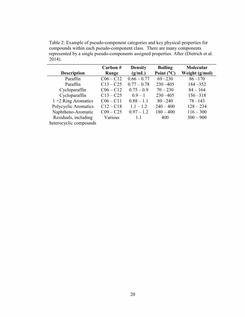
Table 2 presents a typical pseudo-component set and some of the key physical

property ranges associated with the assigned pseudo-component. Of note is the fact

that a very broad set of physical properties is represented within each of the

component groups. This is a frequently used approach, and is generally reasonable

given the variability in crude oil chemical composition, but likely over-generalizes the

physical properties of individual compounds contained in crude oils. Further, this

approach does not account for the impact of external environmental parameters such

as water temperature on the evaporation rate of the material.

The work performed here leverages advances in both computer processing speeds

and analytical methods for determining composition of different crude oils. It

combines the crude oil type composition and percentages of components in concert

18

Figure 3. Crude oil composition as a function of distillation temperature (from Mobil, 1997)

19

Table 1: Typical approximate characteristics and properties of several crude oils

Crude source Paraffins (% vol) Aromatics (% vol) Naphthenes (% vol)

Nigerian - Light 37 9 54

Saudi - Light 63 19 18

Saudi - Heavy 60 15 25

Venezuela - Heavy 35 12 53

Venezuela - Light 52 14 34

USA - W. Texas Sour 46 22 32

North Sea - Brent 50 16 34

20

Table 2: Example of pseudo-component categories and key physical properties for compounds within each pseudo-component class. There are many components represented by a single pseudo-components assigned properties. After (Dietrich et al. 2014).

Description

Carbon #

Range

Density

(g/mL)

Boiling

Point (°C)

Molecular

Weight (g/mol)

Paraffin C06 – C12 0.66 – 0.77 69 –230 86 –170 Paraffin C13 – C25 0.77 – 0.78 230 –405 184 –352

Cycloparaffin C06 – C12 0.75 – 0.9 70 – 230 84 – 164 Cycloparaffin C13 – C25 0.9 – 1 230 –405 156 –318

1 +2 Ring Aromatics C06 – C11 0.88 – 1.1 80 –240 78 –143 Polycyclic Aromatics C12 – C18 1.1 – 1.2 240 – 400 128 – 234 Naphtheno-Aromatic C09 – C25 0.97 – 1.2 180 – 400 116 – 300 Residuals, including

heterocyclic compounds Various 1.1 400 300 – 900

21

with individual chemicals and chemical properties in order to provide a dynamic,

environmentally linked fate and transport model for spilled oil. Chemical composition

is determined continuously throughout a modeling simulation. With this information,

it is then possible to better define the evolution of bulk oil properties and capture the

impact of changes to the bulk properties on the weathering of the oil.

A simplified methodology was adopted to assign and refine a generic crude oil

composition. A list of compounds commonly found in crude oil was compiled based

on investigation of several different published compositions (Ryerson et al. 2012;

Reddy et al. 2012; Sørheim et al. 2011; Leirvik & Myrhaug 2009), and used as the

basis for developing a generic crude oil composition. The relative amounts of the

identified compounds or pseudo-component classes in un-weathered oils from the

Macondo Deepwater Horizon Spill (Reddy et al. 2012; Ryerson et al. 2012), Gjøa

crude oil (Sørheim et al. 2011), and several crude oils that make up the Alvheim blend

(Leirvik & Myrhaug 2009) were compiled and averaged to develop the preliminary

generic composite oil for saturate and aromatic component classes.

Bulk Oil Properties

The bulk properties of immediate interest to the fate and transport of spilled oil

are density, viscosity, and surface tension. These properties control the fate and

transport of spilled oil through their impact on slick spreading and the overall transfer

of evaporating components. In the modeling framework, all three of these properties

22

were initially determined at each timestep as the instantaneous mass or mole weighted

sums of the partial contributions of the individual chemical property and the amount of

that material present:

#$%&'$()*+,- = .(01∗31).01 (4)

where:

Mi is the mass or moles of constituent i, and

Pi is the constituent property of interest for constituent i

In order to generate the bulk properties for crude oil, physical properties were

needed for both the asphaltene and resin components. Density, viscosity, and surface

tension values for the generic asphaltene and resin constituents are compiled based on

literature information on these complex component classes (Da Silva (2001), Wu and

Prausnitz (1998)). There is significant uncertainty in these numbers, as asphaltenes

extracted from crude oils are described as ‘friable solids’, and the liquid range

viscosity value may have been derived, themselves, to fit a model for physical

properties (M. Greenfield, personal communication, April 22, 2016).

23

Table 3: Basic properties of asphaltene and resin constituents, derived from Da Silva (2001) and Wu and Prausnitz (1998) at 25 °C.

Property Asphaltene Resin

Density (kg m-3) 1120 1080 Viscosity (mPa.s) 2.24 1.728 Surface Tension (dyne cm-1) 28 30 Molecular Weight 750 800

24

The accuracy of the calculated general bulk property depends on defining

appropriate temperature dependent values for the individual constituents. Literature

data are generally compiled for standard temperature and pressure conditions, and

often this is not appropriate for environmental conditions. To this end, temperature

dependent surface tension and viscosity empirical fit equations were applied to the

chemical constituents where the data could be located. Individual chemical viscosity

and surface tension algorithms were implemented to allow for temperature-specific

values where data or fitting coefficients were available. The methods for calculating

the temperature adjusted values for viscosity and surface tension values are detailed in

the following sections.

Density

Although density is also temperature dependent, the availability of fitting

coefficients for the crude oil constituents was limited. A temperature correction was

thus not performed.

Surface Tension

The temperature dependent surface tension of the individual oil constituents was

calculated using one of two methods where fitting coefficients were available: the full

or the condensed version of the Design Institute for Physical Properties Research

(DIPPR) 106 regression equation (DDBSP, 2014). The full equation is,

5 (6)7'/9:) = � (1 − �=) �> ? � �@ ? �A�@ ? �B�@A (5)

25

where:

�= = C:DE'7( �':&'$F(G$' (H)�$E(E9FI �':&'$F(G$' (H) and

Cx is to an empirically derived fitting coefficient.

The abbreviated DIPPR equation is:

5 (6)7'/9:) = � (1 − �=) �> (6)

with coefficients and variables having the same definitions as above.

Viscosity

Dynamic viscosity is a measure of the internal friction of a moving fluid that

causes adjacent layers to move in parallel but at different speeds (shear flow). The

parameterization of viscosity is fundamental to the dispersive characteristics of the

constituent in the aqueous environment. Specifically, dynamic viscosity is used to

determine the maximum surface area for a spilled oil, as well as the mass transfer of

material via evaporation. Tabulated viscosity constants (kg m-1 s-1) for individual

constituents were compiled for standard temperature and pressure. Several previously

published equation formats were implemented to provide temperature dependency for

the bulk property calculation for viscosity within the model. The identified equation

formats are reviewed in the following paragraphs.

26

Three methods for calculating viscosity were located and implemented to provide

temperature dependent viscosity values for the individual oil constituents. The first is

the extended Andrade equation (DDBSP, 2014):

J (9#) = 'K&�� ? �>/� ? � � ? �A� (7)

where T is in Kelvin and Cx represents a chemical specific fitting coefficient. The

resulting constituent viscosity is converted to units of kg m-1 s-1 (Pa-s) in order to

align with standard units within the model. There is also an empirically derived

polynomial equation (Infotherm, 2009):

J (LM :�N O�N) = � + �N� + �Q�Q + �R�R (8)

where T is in Kelvin and Cx represents a chemical specific fitting coefficient. Finally,

Yaws (2009) also presented fitting data to calculate the temperature-adjusted

viscosity:

J (LM :�N O�N) = S�10��?U>V ?� �?�A� � (9)

where T is in degrees Kelvin, Cx represents a chemical specific fitting coefficient, and

FC is a unit conversion factor = 0.001.

27

Bulk Density

Bulk density was calculated as the mass-weighted average of the individual crude oil

constituents. Bulk density is calculated at each timestep within the model, accounting

for composition changes in the resultant density value. Although individual

constituent data is largely reported at 25 °C, crude oil density is more often reported at

15 °C. In order to convert empirical results to a reference temperature to test the

individual constituents, Manning and Thompson’s equation to adjust crude oil density

to a temperature other than 15 °C was used:

WX� = WXNY − 5.93 × 10�^ ∗ (�(°�) − 15) (10)

where:

WX� = W&'9E`E9 M$FaE() %` F MEa'7 9$G6' %EI F( (ℎ' 6'OE$'6 (':&'$F(G$' °� WXNY = W&'9E`E9 M$FaE() %` F MEa'7 9$G6' %EI F( 15 °� �(°�) = �':&'$F(G$' E7 6'M$''O �'IOEGO

Bulk Viscosity

Estimation of bulk crude oil viscosity is a challenging task and has been the source of

significant investigation (Quiñones-Cisneros et al. 2001a; Quiñones-Cisneros et al.

2001b; Quiñones-Cisneros et al. 2004; Baylaucq et al. 2006; Quiñones-Cisneros &

Deiters 2006; Quiñones-Cisneros et al. 2008; Quiñones-Cisneros et al. 2015).

Methods that calculate viscosity as a function of density are potentially subject to

additional errors if the density is not measured, as is the case for this work.

Additionally, the viscosity of oils varies greatly as a function of gas content. Dead oil

– oil with no gas content – viscosity correlations have very different dependencies

28

than live oils – freshly released oil from a reservoir with significant gaseous

components. Very heavy oil (density greater than 1000 kg m-3) viscosity correlations

between calculated and measured values are also different from heavy, medium, and

light crude oil viscosities. For the purposes of this work, it was assumed that the oils

were all dead.

Several methods for calculating the bulk viscosity of crude oil were

investigated for agreement with empirical data and use within the model. The first

approach was the simple mass-weight contribution approach described above. The

second method was to apply the Beal method (Beal, 1970) to calculate oil viscosity

(c) as a function of temperature (T, °F) and bulk density as follows:

c = 0.32 + �N.e × N f�3gB.hA � � Ri

�?Q �j (11)

where:

a = 10k .^R? �lAAmno �p

C#q = 141.56'7OE() − 131.5

with density in units of g/mL.

The final method was to use the linear friction theory method developed and

proposed by Quiñones-Cisneros et al. (2000, 2001a, 2001b, 2004, 2006, 2008).

Briefly, this approach posits that viscosity can be treated as the sum of two

components: the dilute gas viscosity (Jsjt) of a constituent and the residual friction

viscosity (Ju):

29

J = Jsjt + Ju (12)

The friction component, in turn can be expanded to include an attractive and repulsive

term similar to pressure in cubic equations of state:

Ju = Jj + J= (13)

The attractive and repulsive friction contributions are related to the attractive and

repulsive pressure contributions to a system by friction coefficients (K) as follows:

Ju = vj&j + v=&=+ v==&=Q (14)

Further research by Quinones (Quiñones-Cisneros et al. 2003) resulted in a

modification to the original approach, and suggested that by implementing a

corresponding states approach, reduced friction (Ju) can be defined as:

Ju = xyx� (15)

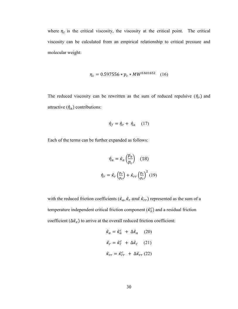
30

where Jz is the critical viscosity, the viscosity at the critical point. The critical

viscosity can be calculated from an empirical relationship to critical pressure and

molecular weight:

Jz = 0.597556 ∗ &z ∗ }~ .i NiYQ (16)

The reduced viscosity can be rewritten as the sum of reduced repulsive (J=) and

attractive (Jj) contributions:

Ju = J= + Jj (17)

Each of the terms can be further expanded as follows:

Jj = vj k&j&z p (18)

J= = v= ��@�� + v== ��@��Q (19)

with the reduced friction coefficients (vj , v= F76 v==) represented as the sum of a

temperature independent critical friction component (v�z) and a residual friction

coefficient (∆v�) to arrive at the overall reduced friction coefficient:

vj = vjz + ∆vj (20)

v= = v=z + ∆v= (21)

v== = v==z + ∆v== (22)

31

The residual friction coefficients can be calculated as a function of critical temperature

and critical pressure using the set of equations:

∆vj = vj, , (Γ − 1) + �vj,N, + vj,N,N�� ∗ ('K&(Γ − 1) − 1) + �vj,Q, + vj,Q,N� +vj,Q,Q�Q � ∗ ('K&(2Γ − 2) − 1) (23)

∆v= = v=, , (Γ − 1) + �v=,N, + v=,N,N�� ∗ ('K&(Γ − 1) − 1) + �v=,Q, + v=,Q,N� +v=,Q,Q�Q � ∗ ('K&(2Γ − 2) − 1) (24)

∆v== = v=,Q,N� ∗ ('K&(2Γ) − 1)(Γ − 1)Q (25)

where:

Γ = �� , and

� = ��z&z

Quinones-Cisñeros (2001a) examined the individual coefficients contained within

these equation and proposed a universal set of constants that could be applied for

determining the residual friction components and the critical reduced friction

parameters, as a function of the equation of state used. The Peng-Robinson, Stryjek-

Vera Equation of State (PRSV-EOS) was used as the method for comparing bulk

viscosity calculations. The PRSV-EOS is well suited to hydrocarbons and is widely

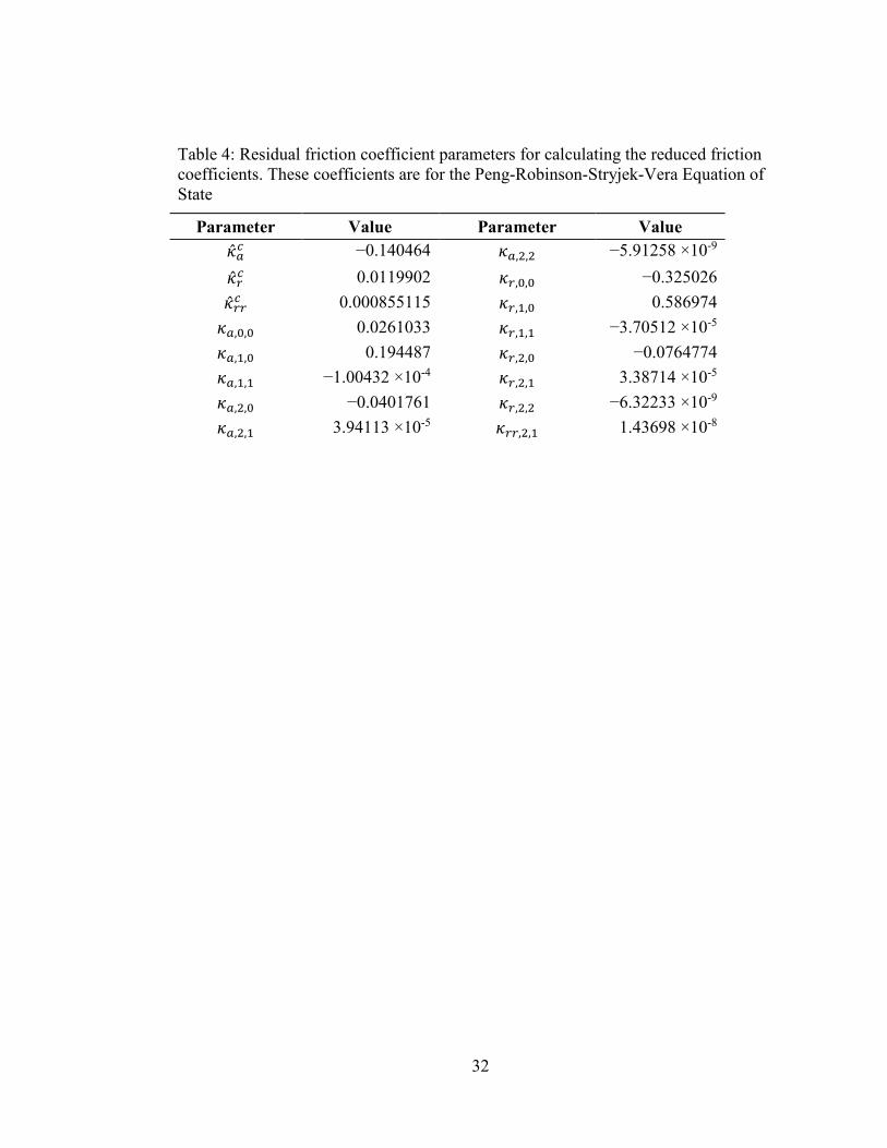
used in the determination of the hydrocarbon mixture properties. Table 4 displays the

residual and fitted individual friction coefficients that correspond to the PRSV-EOS.

32

Table 4: Residual friction coefficient parameters for calculating the reduced friction coefficients. These coefficients are for the Peng-Robinson-Stryjek-Vera Equation of State

Parameter Value Parameter Value vjz −0.140464 vj,Q,Q −5.91258 ×10-9

v=z 0.0119902 v=, , −0.325026

v==z 0.000855115 v=,N, 0.586974 vj, , 0.0261033 v=,N,N −3.70512 ×10-5 vj,N, 0.194487 v=,Q, −0.0764774 vj,N,N −1.00432 ×10-4 v=,Q,N 3.38714 ×10-5 vj,Q, −0.0401761 v=,Q,Q −6.32233 ×10-9 vj,Q,N 3.94113 ×10-5 v==,Q,N 1.43698 ×10-8

33

Viscosity values for each component were calculated and summed to develop a

mass based mixture value for the dilute gas and friction components:

J�� = J ,�� + Ju,�� (26)

where:

J ,�� = 'K& �� K�ln�J ,N��

��N�

Ju,�� = 'K& �� K�ln�Ju,N��

��N�

The friction contribution mixing rules used for this work were a slight departure from

that implemented by Quinones-Cisneros, as the weighted mixing method proposed

could not be easily implemented in a dynamic manner within the proposed modeling

construct. The results of all three viscosity methods are presented in Chapter 4.

Evaporation

A simple evaporation model was implemented to determine the mass flux per

model timestep on a component-by-component basis. Evaporation is the process of

transfer from the liquid phase to the vapor phase, and is applied to non-dissolved

materials above a certain depth in the water column for the purposes of the model.

Within the model, the molar amount of each non-dissolved constituent within the mass

weighted bulk material composite that evaporates at each timestep is calculated in the

following manner:

34

}��j� = S��j� ∗ Ct+=u ∗ ( (27)

where:

t is the model timestep

Asurf is the surface area (m2) of the slick (here parcel of the slick)

Fevap is the calculated evaporative flux (mol m-2 s-1)

Evaporation is calculated as a function of the overall mass transfer coefficient and

the amount of material in the surface oil. A film-based exchange model is used to

determine the net evaporative flux (F) for air-sea exchange .(Deacon 1977) The

overall flux equation is:

S = L(�� − ��) (28)

where:

k = the overall transfer coefficient cm s-1

Cw = the concentration of the material in the water (oil phase for the model)

Ceq = the equilibrium atmospheric concentration.

Because the atmosphere is an open-ended boundary, the equilibrium

concentration above the air-water interface can be effectively ignored, simplifying the

equation to the following:

S = L ∗ �� (29)

35

The overall transfer coefficient (k) is calculated as function of the air-phase and

water-phase diffusivities (Deacon 1977):

N-��@�� = N

��1@�

�� + N��@ (30)

where:

vwater = the exchange velocity in water (cm s-1) for a given constituent

vair = the exchange velocity in air (cm s-1)

H = the Henry’s Law Constant (m3 atm mol-1)

R = the ideal gas constant, here 8.21 ×10-5 m3 atm mol-1 K-1

T = Temperature (Kelvin)

The flux determination is based on the combined air-phase and water-phase

exchange velocities. The air-phase velocity is based on the methodology of MacKay

and Yeun (1983), and is related to the exchange velocity of water:

aj�= = k �1�� p .i� a�j��=,j�= (31)

where:

vair = the velocity of the substance in air (cm s-1)

Dia – the diffusivity of the compound of interest in air (cm2 s-1)

DH2O = the diffusivity of water vapor in air (cm2 s-1)

vwater,air = the velocity of water vapor in air (cm s-1)

36

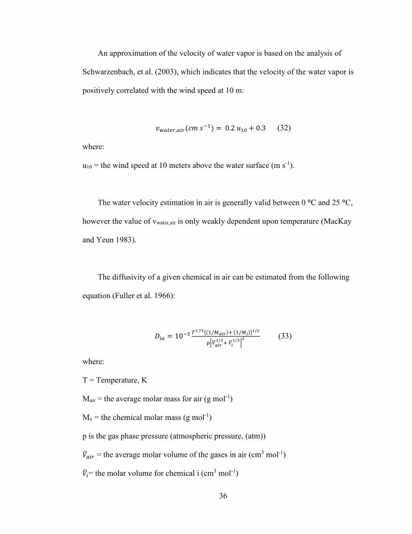
An approximation of the velocity of water vapor is based on the analysis of

Schwarzenbach, et al. (2003), which indicates that the velocity of the water vapor is

positively correlated with the wind speed at 10 m:

a�j��=,j�=(9: O�N) = 0.2 GN + 0.3 (32)

where:

u10 = the wind speed at 10 meters above the water surface (m s-1).

The water velocity estimation in air is generally valid between 0 °C and 25 °C,

however the value of vwater,air is only weakly dependent upon temperature (MacKay

and Yeun 1983).

The diffusivity of a given chemical in air can be estimated from the following

equation (Fuller et al. 1966):

�j = 10�R �>.fh¡(N/0�1@)? (N/01)¢>/ �£�¤�1@>/A? �¤1>/A¥ (33)

where:

T = Temperature, K

Mair = the average molar mass for air (g mol-1)

Mx = the chemical molar mass (g mol-1)

p is the gas phase pressure (atmospheric pressure, (atm))

¦§j�= = the average molar volume of the gases in air (cm3 mol-1)

¦§�= the molar volume for chemical i (cm3 mol-1)

37

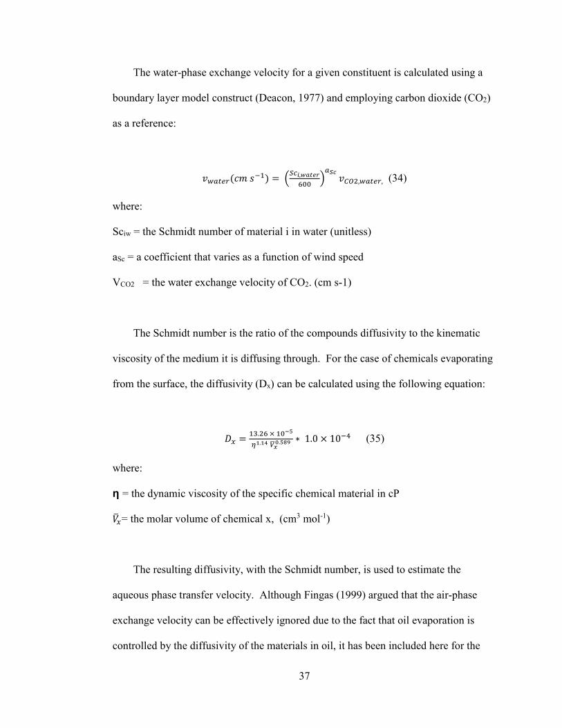
The water-phase exchange velocity for a given constituent is calculated using a

boundary layer model construct (Deacon, 1977) and employing carbon dioxide (CO2)

as a reference:

a�j��=(9: O�N) = �¨z1,��@i �j©� a�ªQ,�j��=, (34)

where:

Sciw = the Schmidt number of material i in water (unitless)

aSc = a coefficient that varies as a function of wind speed

VCO2 = the water exchange velocity of CO2. (cm s-1)

The Schmidt number is the ratio of the compounds diffusivity to the kinematic

viscosity of the medium it is diffusing through. For the case of chemicals evaporating

from the surface, the diffusivity (Dx) can be calculated using the following equation:

� = NR.Qi × N «hx>.>B �¤¬�.hl ∗ 1.0 × 10�^ (35)

where:

η = the dynamic viscosity of the specific chemical material in cP

¦§�= the molar volume of chemical x, (cm3 mol-1)

The resulting diffusivity, with the Schmidt number, is used to estimate the

aqueous phase transfer velocity. Although Fingas (1999) argued that the air-phase

exchange velocity can be effectively ignored due to the fact that oil evaporation is

controlled by the diffusivity of the materials in oil, it has been included here for the

38

sake of completeness. Table 5 presents the water-controlled (Water Only), air

controlled (Air Only), and combined (Water + Air; Water) transfer velocity

coefficients for three representative crude oil constituents. In each case presented, the

air exchange velocity is significantly faster than the water oil exchange velocity,

supporting the case made by (Fingas 2011) that exchange would be water oil limited

rather than air limited. The final column in the table calculates the overall exchange

using the viscosity of Arabian Light Crude (931 mPa.s at 20 °C) to determine a

representative overall transfer coefficient for each of the constituents within crude oil.

In all cases, the overall transfer coefficient calculation results in a lower value in crude

oil, further supporting the liquid (water or oil) -controlled case. For higher viscosity

constituents, the contribution from air exchange begins to become a more significant

portion, due to the relatively low diffusivity.

39

Table 5: Examples of overall transfer velocity coefficients based on water-controlled exchange (Water Only), Air-controlled exchange (Air only), and the combination of the two for three different crude oil constituents for pure components and within Arabian Light Crude Oil (Oil).

Compound

Water Only

V (cm s-1) Air Only

(cm s-1) Water + Air

(cm s-1) Water + Air,

Oil (cm s-1)

Pentane 0.0815 12.9 0.00810 1.19x 10-5 Benzene 0.000922 0.0777 0.000912 1.65 x 10-5

Naphthalene 0.000117 0.000463 0.0000935 1.55 x 10-5

40

Application of Heat Budget Information

Most modeling systems do not implement methods to meticulously account for

how much of the available energy that can be used for evaporation is utilized in

evaporating materials from the sea surface. By not tracking this information, there is

the potential to evaporate oil far more quickly than realistically could be expected. To

avoid this potential pitfall, modeling methods were developed to check the energy

used for evaporation and balance it according to the available net longwave radiation.

Surface net upward longwave radiative flux data for the oceans was acquired from

NOAA NCEP/NCAR reanalyzed monthly averaged climatological data (1981-2010)

(NOAA/ORA/ESRL PSD). This data is publicly available, and the spatial data

resolution is 2.5 degrees. Figure 4 presents global long-term monthly longwave

radiative flux data for January (top) and July (bottom). Note the variations in the

scales for the figures. The estimated material flux for a given chemical is converted to

the energy needed to evaporate it using the chemical specific latent heat of

vaporization. The total energy needed is subtracted for the surface area adjusted

longwave radiation for the model timestep. When the energy needed exceeds the

available energy, the amount of material that can evaporate is reduced to equal the

available energy. After this point, no more evaporation can occur for a given particle

in the model. The energy requirements for evaporation of a given chemical mass is

calculated as:

®7'$M) �'¯GE$'6 (°%GI'O) = :%I'O�t��j��± ⋆ ³´�j� (36)

where:

41

molesestimated = the theoretical amount of material that could be evaporated (moles)

³´�j� = the enthalpy of vaporization (joules mol-1) for the individual chemical

The energy required to evaporate the amount of a compound is then compared to

the area and time-adjusted data from the seasonal profile database, a compilation of

geo-referenced set of data that includes temperature, salinity, and values for net

longwave radiation at that location as:

®7'$M) CaFEIFDI' (°%GI'O) = µ~��(~ :�Q) ⋆ C$'F¨¶�·(:Q) * timestep (37)

The required energy to evaporate material from the oil is subtracted from the total

available energy for the slick surface area as the individual components are

evaporated. If the required energy exceeds the available energy, the amount of

material evaporated is limited as:

}%I'O¸��3 = ¸��=s¹ ��j�,jº,� (»)¼�� (38)

Within the modeling framework, each chemical is subject to chemical specific

calculated rates for evaporation. It is not possible to specify the order in which

chemicals are queued up to execute the evaporation algorithms within the model. In

practice, this means that a less volatile component may be subjected to evaporation

within the model before a more volatile component. This does not appear to be a

42

Figure 4: Monthly mean surface upward longwave radiation flux (W m-2) for January (top) and July (bottom). Images created from NCEP reanalysis derived data (NOAA/ORA/ESRL PSD)

43

significant problem with model output, as the most volatile components will account

for the largest share of energy consumption for evaporation. The result is that the

implementation of the energy limitation is minimally impacted by the inability to

determine the order of chemical evaporation, due to the theoretical maximum

evaporation limit being much smaller for the least volatile components. The

theoretical throttling by available energy that would be encountered within the model

would thus be applied to the most volatile components that are evaporated first based

on the model order. Once they were completely evaporated out of solution, the next

most volatile component(s) would no longer be subjected to an energy barrier to

evaporate. Generally speaking, after the first few timesteps of a model run, the most

volatile components have evaporated out of the crude oil, and there is no longer an

energy supply limitation on the overall crude oil evaporative flux.

Slick Spreading

Once the bulk properties were determined, slick spreading rates were determined

using gravitational and viscous forcing. This is accomplished by implementing the

original equations of Fay (1969, 1971). The length of the slick from the center is

determined as a function of time according to the following:

I'7M(ℎ(:) = 1.5 £��½�� 1��½� � ∗ � �>.h��.h ¥ .QY

(39)

where:

�t� = the density of seawater, or the surrounding water

44

�¾�, = the density of the released oil

t = time (hours)

ν = the kinematic viscosity of the released oil (mPa.s)

A = the maximum surface area of the oil slick, calculated as (Fay 1969):

C(:Q) = 10Y¡¦¢ .�Y (40)

where:

V = the volume of released oil (m3)

The thickness of the spilled oil is then computed by dividing the volume of oil by the

surface area. Although this assumes that the thickness is essentially uniform, the

Lagrangian modeling approach applies the thickness calculation on a particle-by-

particle basis, so particles of different ages or composition would have different

thicknesses.

Emulsification

The final component of the modeling approach was to use the calculated physical

and bulk properties to assess the emulsion state. Fingas (2010) proposed a set of

criteria that contribute to the formation of the stability categories of crude oil

emulsions. The four general categories of emulsions – stable, meso-stable, entrained,

and unstable – vary by viscosity, resin, and asphaltene composition (Figure 5), with

some overlap between categories. Stable emulsions can contain up to 80% water and

persist for months to years while unstable emulsions do not contain a significant

45

amount of water and do not persist. Fingas further refined this concept and found

better agreement between the predicted emulsion state and empirical observations

(Fingas 2014).

The time varying bulk properties and the asphaltene: resin ratio from the multi-

component evaporation model were used to characterize a spilled oil relative to the

empirical observations (Fingas 2011; M. Fingas 2014). Once the oil was found to be in

a stably emulsified state, evaporation ceased to be a major loss term, slick spreading

was assumed to be negligible, and, depending on the resulting density, wind-driven

surface transport was no longer be applied. Cessation of weathering processes and

surface slick drift was implemented as a result of the uncertainty in calculating

evaporation due to the presence of water, and the potential for the emulsion to be

neutrally buoyant, and thus sub-surface.

The oil emulsion state was determined by calculating a Stability factor (F. Fingas

2014) as follows:

W(FDEIE() = 5667 + 9520 ∗ � − 3.99 ∗ ¦� + 0.138 ∗ W� ∓ 0.216 ∗ ��

− 0.395 ∗ C + 17.9 ∗ �� + 224 ∗ exp(�) + 2.88 × 10�N ∗ exp(��) − 4.35 ∗

exp � �� + 16823 ∗ ln(�) + 10.5 ∗ ln(¦�) − 0.671 ∗ log(W�) + 0.147 ∗ ln(��) +

0.107 ∗ ln(C) + 1.62 ∗ log � �� (41)

where:

46

W� is the transformed saturate content. If the percent saturate content is less that 45%, the value is equal to 45 minus the percent saturate content, otherwise it is the percent saturate content minus 45.

�� is the transformed resin content. If the percent resin content is less that 10%, the value is equal to 10 minus the percent resin content, otherwise it is the percent resin content minus 10. If the resin content is equal to zero, this value is set to 20.

C�is the transformed asphaltene content. If the percent asphaltene content is less that 4%, the value is equal to 4 minus the percent resin content, otherwise it is the percent asphaltene content minus 4. If the asphaltene content is equal to zero, this value is set to 20.

C/R is the asphaltene to resin ratio, calculated as the percent asphaltene divided by the percent resin content (A/R).

¦� is the transformed viscosity, the natural log of the viscosity in (mPa.s) .

ρ is the exponential of density (g mL-1).

The computed stability value is compared to the following criteria (

Table 6), and used to determine the oil emulsion state.

Each of these emulsion states has a typical percentage of water and oil, as

described in Table 7. These percentages are used to determine density, viscosity, and

surface tension of spilled oil when it has weathered but is no longer actively

evaporating. Only the “not emulsified” state is subject to all degradation processes and

additional surface wind driven transport in the model.

Figure 5 presents the emulsion types graphically as a function of viscosity and the

product of resin and asphaltene content.

47

The emulsification state algorithm, as implemented in the model, utilizes

calculated bulk density and viscosity values that include the impact that calculated

changes in these properties have on the individual constituent evaporation rates. By

re-determining the bulk properties at each time step, the model affords calculated

evaporation rates that can also incorporate changes in the external temperature of the

surrounding seawater and the effects that these dynamic rates have on the overall

crude oil bulk properties. By implementing the algorithms in this fashion, the

emulsification state calculation is also linked to available environmental conditions.

48

Table 6: Emulsion state determination matrix, modified from Fingas, 2014

Calculated

Stability Value

Minimum

Calculated

Stability Value

Maximum

Other Conditions

State

2.2 15 None Stable

-12 -0.7 None Meso-stable

-18.3 -9.1 density > 0.96 g mL-1 viscosity > 6000 mPa.s

Entrained

-7.1 -39.1 density >0.85 or < 1 g mL-1

viscosity > 800000 or < 10 mPa.s

Unstable

49

Table 7: Oil and water percentages for the various emulsion states

Emulsion State % Oil % Water

Not Emulsified 100 0

Stable 20 80

Meso-Stable 35 65

Unstable 95 5

Entrained 70 30

50

Figure 5: Viscosity and composition ranges for the 4 main emulsion types (Fingas and Lyman, 2011)

51

CHAPTER 4

RESULTS AND DISCUSSION

The bulk property method calculations described in Chapter 3 were

investigated for suitability within the modeling framework. To apply the best possible

emulsification state algorithm, the goal for method selection was to best represent

empirical data. To that end, the bulk density and bulk viscosity methods were

compared to empirical properties and the resulting emulsification state compared to

published data (Fingas 2011; Fingas 2014).

Bulk Density Estimates

Fingas (2011, 2014) presented an extensive list of oil compositions with

corresponding emulsification states as a function of weathering to test the validity of

his emulsification state calculation. The same stability algorithm was implemented

within the model proposed in this work. The emulsification state stability algorithm is

strongly dependent upon both density and viscosity, and a comparison of the model

calculated density to empirical density was done to determine how well the crude oil

composition and bulk property calculation represented actual crude oil density. When

density data from 25 °C was not available for the oils investigated, empirical oil

densities at 15 °C in (Fingas 2014) were converted to 25 °C and compared to

estimated crude oil density at 25 °C using the method of (Manning & Thompson

1995). The adjustment was done to confirm the composition appropriateness as the

majority of density values for individual constituents are reported at 25 °C. This is

52

also the case for non-fitted viscosity data. Density and viscosity at two temperatures

can then be used to estimate viscosity at a third temperature when empirical

information is unavailable. Density values at 25 °C were calculated using Manning

and Thompson’s method (Equation 11). Crude oil API values ranged from extra heavy

(API < 10, density > 1000 kg m-3) to extra light (API> 40, density < 825 kg m-3).

Empirical or temperature adjusted density for non-weathered oils was then

compared to model calculated density. Figure 6 shows the preliminary regression fit

for model predicted values versus the reported density values for 110 different un-

weathered oils. The equation for the linear regression of the model predicted density

values versus empirical density values suggests that using the generic oil composition

list and varying the percentages of the saturates, aromatics, resins, and asphaltenes can

represent crude oil density values fairly well (R2 = 0.90083, Figure 6). The initially

proposed saturate content generally under predicted crude oil density for lower density

crude oils, but showed a slightly better fit for higher density crude oils, where the

aromatic, resin, and asphaltene amounts in the crude oils were somewhat higher.

To investigate improving the fit between empirical and model calculated density

values, the relative composition of the saturate content was modified to shift towards

higher molecular weight compounds. The preliminary composition resulted in an

average saturate density value of 727 kg m-3. A shift in composition towards

decreased content below C6 hydrocarbons resulted in an average saturate density of

53

749 kg m-3. A linear regression of the modified saturate content predicted density

compared to the empirical density value (

Figure 7) showed no improvement in the correlation coefficient for the linear

regression of the actual density versus model-calculated density, however the

distribution of data at both low and high density ranges showed model predictions that

were both greater and less than the empirical data, presumably resulting in a better

overall fit of the data, with the slope of the linear fit of the modified saturate content

somewhat closer to 1 (0.8886 vs. 0.8257). Another iteration of composition

modifications in the saturate content towards a slightly more dense composition

(Figure 8) showed a slope closer to unity (0.9847) with an intercept of 0.0146. A

comparison of actual and predicted values using the slope and intercepts for each of

the three saturate density linear fit regression equations (Tab le 8) suggests that the

highest density saturate composition results in data closer to anticipated results – i.e. –

the resulting density agrees better with empirical values for the crude oils examined

when assigning the initial, empirical density as the independent variable and

calculating the expected density. The relative error in the slope of the three separate

iterations was assessed in an attempt to identify the best overall fit, however the results

were essentially the same (3.5% – 3.6%).

The results indicate that, overall, the density values that result from assigning

component fraction percentages agree reasonably well with observations: Relative

errors in the density calculations were generally less than 5%, with model calculations

over and under predicting oil bulk density values (Table 6). The final generic crude oil

54

composition with relative percentages within each major component class is presented

in Appendix 1.

55

Figure 6: Comparison of actual oil density and model predicted density (g/mL) for un-weathered oils. Saturate density 0.727 g mL-1. The dark line in the figure is the ideal slope of a linear fit of unity. The relative error of the slope and intercept are 3.3% and 26.7%, respectively.

56


57


58

Table 8: Comparison of model predicted density for each of the saturate density values using the resultant linear least square slope and intercept. The adjusted saturate density of 780 kg m-3 showed the best overall fit across a range of crude oil densities.

Saturate

Density

727

(kg m-3)

Saturate

Density

749

(kg m-3)

Saturate

Density

780

(kg m-3)

Calculated Density, Actual Density = 750 kg m-3 804 787 753 Calculated Density, Actual Density = 800 kg m-3 845 831 802 Calculated Density, Actual Density = 850 kg m-3 887 876 851 Calculated Density, Actual Density = 900 kg m-3 928 920 900 Calculated Density, Actual Density = 950 kg m-3 969 965 950 Calculated Density, Actual Density = 1000 kg m-3 1011 1009 999

59

Table 9: Comparison of model calculated density to a subset of empirical density data from (Fingas 2011; Fingas 2014)

Oil

Saturate %

Resin %

Asphaltene %

Density

empirical

(kg m-3)

Density

(model)

(kg m-3)

Arabian Light 51 6 3 859.9 878.3

Arabian Med 55 7 6 872.4 879.7

Canolimon 60 8 8 873.8 872.5 Hondo 33 24 12 929.7 946.2 Lago Treco 38 14 11 917.1 924.7 Lucula 62 9 4 851.5 855.3

Neptune Spar 58 19 10 861.3 849.2

Platform Gail 39 21 12 922.4 932.1

Point Arguello Comingled

36 23 16 918.9 946.8

Sockeye 48 13 8 890.6 899.4

Sockeye Comingled

34 21 13 930.3 942.4

Sockeye Sour 38 20 13 936.2 935.1

Takula 65 8 2 857.8 858.7 MC 807 47 12 6 883.0 896.4 Prudhoe Bay 1995

53 10 4 877.8 881.8

Santa Clara 36 29 13 914.3 949.3

Sockeye 2000 50 18 15 929.5 918.4

60

Bulk Viscosity Predictions

The mass-weighted chemical constituent viscosity values were tested to derive a

composite bulk viscosity for crude oil using the identified subset of constituent

chemicals. A comparison of the calculated values to empirical data from (Fingas

2011; Fingas 2014) (

Table 10) showed very poor agreement for oils with resin content above 14%.

This is partly due to the complex interaction of asphaltenes with the aromatic

components in oil, an area that is still under active investigation. It is also the result of

the overly simplistic approach using mass-weighted fractional contributions for

calculating bulk viscosity.

Although altering the viscosity of the resin constituent to match the derived

data would seem to resolve the problem for the grossest discrepancies in viscosity, as

is the case for Santa Clara and Sockeye 2000 crude oils, this resulted in an increase in

the discrepancy for lower viscosity oils. Also, in scrutinizing the results, the model

predicted result for Arabian Light and Arabian Medium crude oil suggest that the

discrepancy is in the calculation of the saturate contribution to the bulk viscosity. The

saturate percentages for Arabian Light and Arabian Medium crude oil respectively, are

51% and 55%, with actual viscosity values of 9.1 and 19.5 mPa.s. The model

calculated viscosity results in Arabian Medium with a slightly lower viscosity of 24.2

mPa.s than Arabian Light (29.7), the opposite of the empirical results. It is possible

that one or more of the saturate constituents has an error in the fitted viscosity

61

coefficients, resulting in the inconsistent value being amplified with increasing

saturate content.

The Beal method (Beal, 1970) was also tested to calculate dead oil viscosity (c)

as a function of temperature (T, °F) and API gravity based on the adjusted crude oil

density. Table 10 and

Figure 9 present empirical data and the simple bulk viscosity calculation and the

Beal method to the published empirical viscosity values. The Beal method performed

better than the simple method for the highest density oils, but did not perform better

than the simple method for high API gravity values (low density) oils based on a linear

regression of the predicted and empirical data. Implementation of the Beal method did

not resolve the viscosity discrepancies for Sockeye 2000 that are largely the reason

that the model predicts the formation of a stable emulsion (Table 11).

Table 10 also contains the friction theory viscosity methodology results. This

method does a better job at matching higher viscosity oil than the simple mass-

weighted approach, providing a moderate means for estimating viscosity that can

match lower and moderate viscosities well. The fact that it is based on constituent

properties, assuming they are well represented, argues for using the friction viscosity

method over the Beal method, although the Beal results show a reasonable fit for the

subset of data investigated.

Table 11 presents a comparison of the observed and model predicted emulsion

states for the subset of oils investigated. The model replicated observed emulsification

states in 14 of the 17 oils investigated. Discrepancies in the timing of the onset of

62

emulsification are discussed in the next section. The observed results suggest that the

proposed model, even with the observed discrepancies in viscosity, is useful for

predicting the ultimate emulsification state.

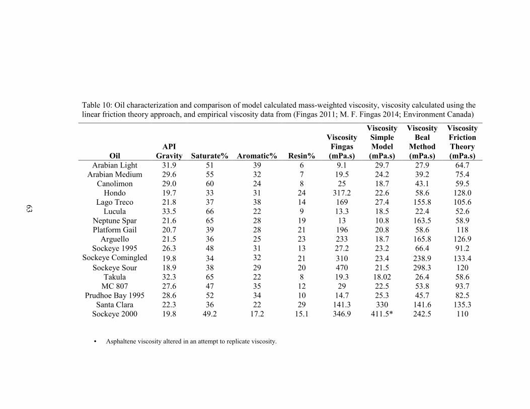
63

Table 10: Oil characterization and comparison of model calculated mass-weighted viscosity, viscosity calculated using the linear friction theory approach, and empirical viscosity data from (Fingas 2011; M. F. Fingas 2014; Environment Canada)

• Asphaltene viscosity altered in an attempt to replicate viscosity.

Oil

API

Gravity

Saturate%

Aromatic%

Resin%

Viscosity

Fingas

(mPa.s)

Viscosity

Simple

Model

(mPa.s)

Viscosity

Beal

Method

(mPa.s)

Viscosity

Friction

Theory

(mPa.s)

Arabian Light 31.9 51 39 6 9.1 29.7 27.9 64.7 Arabian Medium 29.6 55 32 7 19.5 24.2 39.2 75.4

Canolimon 29.0 60 24 8 25 18.7 43.1 59.5 Hondo 19.7 33 31 24 317.2 22.6 58.6 128.0

Lago Treco 21.8 37 38 14 169 27.4 155.8 105.6 Lucula 33.5 66 22 9 13.3 18.5 22.4 52.6

Neptune Spar 21.6 65 28 19 13 10.8 163.5 58.9 Platform Gail 20.7 39 28 21 196 20.8 58.6 118

Arguello 21.5 36 25 23 233 18.7 165.8 126.9 Sockeye 1995 26.3 48 31 13 27.2 23.2 66.4 91.2

Sockeye Comingled 19.8 34 32 21 310 23.4 238.9 133.4 Sockeye Sour 18.9 38 29 20 470 21.5 298.3 120

Takula 32.3 65 22 8 19.3 18.02 26.4 58.6 MC 807 27.6 47 35 12 29 22.5 53.8 93.7

Prudhoe Bay 1995 28.6 52 34 10 14.7 25.3 45.7 82.5 Santa Clara 22.3 36 22 29 141.3 330 141.6 135.3

Sockeye 2000 19.8 49.2 17.2 15.1 346.9 411.5* 242.5 110

64

Figure 9: Comparison of Actual Viscosity Values (Fingas) and Model Predicted Viscosity values (mPa.s) for the three methods of bulk viscosity calculations. The dark line in the figure represents a perfect fit between empirical and calculated viscosity.

65

Table 11: Comparison of model calculated emulsification state prediction to empirical emulsion state observations from (Fingas 2011; M. F. Fingas 2014; Environment Canada).

Oil Saturate

% Aromatic

%

Resin

% Asphaltene

% Emulsion

State, Fingas

Emulsion State,

Model

Arabian Light 51 39 6 3 STABLE UNSTABLE Arabian Med 55 32 7 6 STABLE STABLE Canolimon 60 24 8 8 STABLE STABLE

Hondo 33 31 24 12 STABLE STABLE Lago Treco 37 38 14 11 STABLE STABLE

Lucula 66 22 9 4 STABLE STABLE Neptune Spar 65 28 19 10 STABLE STABLE Platform Gail 39 28 21 12 STABLE STABLE

Arguello 36 25 23 16 STABLE STABLE Sockeye 1995 48 31 13 8 STABLE STABLE

Sockeye Comingled 34 32 21 13 STABLE STABLE Sockeye Sour 38 29 20 13 STABLE STABLE

Takula 65 22 8 2 STABLE STABLE MC 807 47 35 12 6 MESOSTABLE STABLE

Prudhoe Bay 1995 52 34 10 4 MESOSTABLE STABLE Santa Clara 36 22 29 13 MESOSTABLE MESOSTABLE

Sockeye 2000* 49.2 17.2 15.1 18.5 MESOSTABLE STABLE * Asphaltene viscosity altered in an attempt to replicate emulsion state.

66

Weathering Rates

The most comprehensive test of the proposed model’s ability to accurately

determine the fate and transport of spilled oil and capture emulsion state is to compare

the model predicted weathering to empirical data. This comparison consisted of

model output over the time period of interest and information from the Environment

Canada oil spill database (ref). Model estimated changes in crude oil bulk properties

as a function of oil weathering state were compared to empirical data for several

different oil types to test the model’s overall ability to replicate observed crude oil

weathering. The output density, mass, viscosity, and emulsification states were

compared to documented laboratory data for 4 different oils: Arabian Light Crude Oil,

Hondo Crude Oil, Santa Clara Crude Oil, and Jet Fuel.

Table 12 shows an abbreviated comparison of empirical data and model

predicted Arabian Light crude oil properties at 3 stages of weathering. The mass of

Arabian Light as a function of time as predicted by the model and the Environment

Canada fitted data are presented in Figure 10. The model under-predicts the

evaporation rate during the first hour: 8% model predicted vs. ~12% empirical fitted

value. The model tracks reasonably well with empirical data for the first 7-8 hours,

but after this point the model does not capture the transition to a stable emulsion, and

therefore evaporation continues without the dampening effect observed for meso-

stable and stable emulsions. The model over-predicts the viscosity in the non-

emulsified oil, and under-predicts the viscosity in the stably emulsified oil. Part of the

under-prediction is a function of the time-dependent algorithm implemented for meso-

67

stable emulsion viscosity, suggesting that this algorithm should be revisited.

Additionally, the model predicts an unstable emulsification state for Arabian Light,

whereas the empirical data suggest a stable emulsion is formed.

Hondo crude oil was also used to compare model predictions to empirical data.

Model output shows comparable results for time to evaporation. The model predicts

17% weathering of Hondo crude at 6 hours, whereas empirical results suggest 17%

weathering is reached at 11 hours (Table 13, Figure 11). The fitted equation predicts

34% oil weathering at 134 hours. The model does not achieve 34% weathering of the

oil because the evaporation algorithms are not implemented within the model once a

stable emulsion forms. The weathered viscosity values show better agreement for the

partially weathered oil than for the Arabian Light crude, but the implemented viscosity

algorithm under-predicted the weathered oil viscosity again. This may be due to the

inability to select the evaporation order in the model, causing an under-prediction of

the initial calculated evaporation rate. Density values show reasonable agreement

between model predictions and empirical observations.

A comparison of Santa Clara crude model predictions with empirical data

shows reasonable agreement for un-weathered and moderately weathered (11%) oil,

with the model capturing the meso-stable emulsion state at 11% weathering (Table 14,

Figure 12). For Santa Clara crude oil, the model predicts a stable emulsion earlier

than it is achieved. The final state of weathered Santa Clara oil is a stable emulsion

(Fingas 2014), however empirical data from Environment Canada show a meso-stable

68

emulsion at 22% weathering. The model determined a stable emulsification state

when the weathering corresponded to 14%.

The weathering of Jet Fuel was well captured by the model formulation, with

53% weathering achieved within 2.5 hours of the anticipated weathering rate from the

Environment Canada empirical observations: The model required roughly 26.5 hours

to reach 53% weathering, whereas the equation derived from empirical data suggested

24.25 hours to reach 53% weathering of the material. The Jet Fuel was comprised of

only saturates and resins, yet the predicted viscosity values were still larger than the

empirical results, further reinforcing the possibility of an error in a saturate constituent

viscosity value.

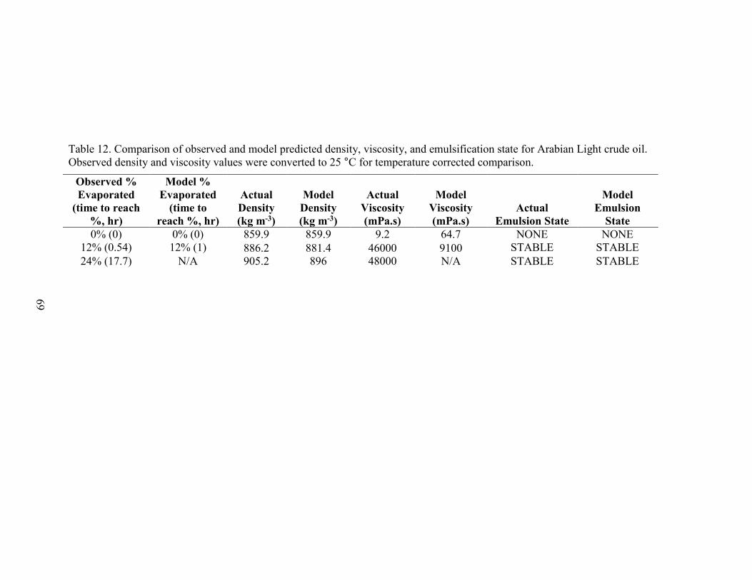
69

Table 12. Comparison of observed and model predicted density, viscosity, and emulsification state for Arabian Light crude oil. Observed density and viscosity values were converted to 25 °C for temperature corrected comparison.

Observed %

Evaporated

(time to reach

%, hr)

Model %

Evaporated

(time to

reach %, hr)

Actual

Density

(kg m-3)

Model

Density

(kg m-3)

Actual

Viscosity

(mPa.s)

Model

Viscosity

(mPa.s)

Actual

Emulsion State

Model

Emulsion

State

0% (0) 0% (0) 859.9 859.9 9.2 64.7 NONE NONE 12% (0.54) 12% (1) 886.2 881.4 46000 9100 STABLE STABLE

24% (17.7) N/A 905.2 896 48000 N/A STABLE STABLE

70

Table 13: Comparison of observed and model predicted density, viscosity, and emulsification state for Hondo crude oil. Observed density and viscosity values were converted to 25 °C for temperature corrected comparison.

Observed %

Evaporated

(time to reach

%, hr)

Model %

Evaporated

(time to

reach %, hr)

Actual

Density

(kg m-3)

Model

Density

(kg m-3)

Actual

Viscosity

(mPa.s)

Model

Viscosity

(mPa.s)

Actual Emulsion

State

Model Emulsion

State

0% (0) 0% (0) 929.67 937.7 341.2 128.0 NONE NONE

17% (11) 14% (6) 961.47 1017.15 2650 1850 STABLE STABLE

32% (143) N/A 982.17 N/A 937.7 N/A STABLE STABLE

71

Table 14. Comparison of observed and model predicted density, viscosity, and emulsification state for Santa Clara crude oil. Observed density and viscosity values were converted to 25 °C for temperature corrected comparison.

*Estimated from 10 m/s shear rate data for 0 and 15 °C

Observed %

Evaporated

(time to reach

%, hr)

Model %

Evaporated

(time to

reach %, hr)

Actual

Density

(kg m-3)

Model

Density

(kg m-3)

Actual

Viscosity

(mPa.s)

Model

Viscosity

(mPa.s)

Actual Emulsion

State

Model Emulsion

State

0% (0) 0% (0) 914.3 939.6 141.3 135.3 NONE NONE

11% (0.92) 11% (1.5) 942.0 954.6 516 189.2 MESO MESO

22% (143) N/A 961.3 954.6 13105* 1200 MESO STABLE

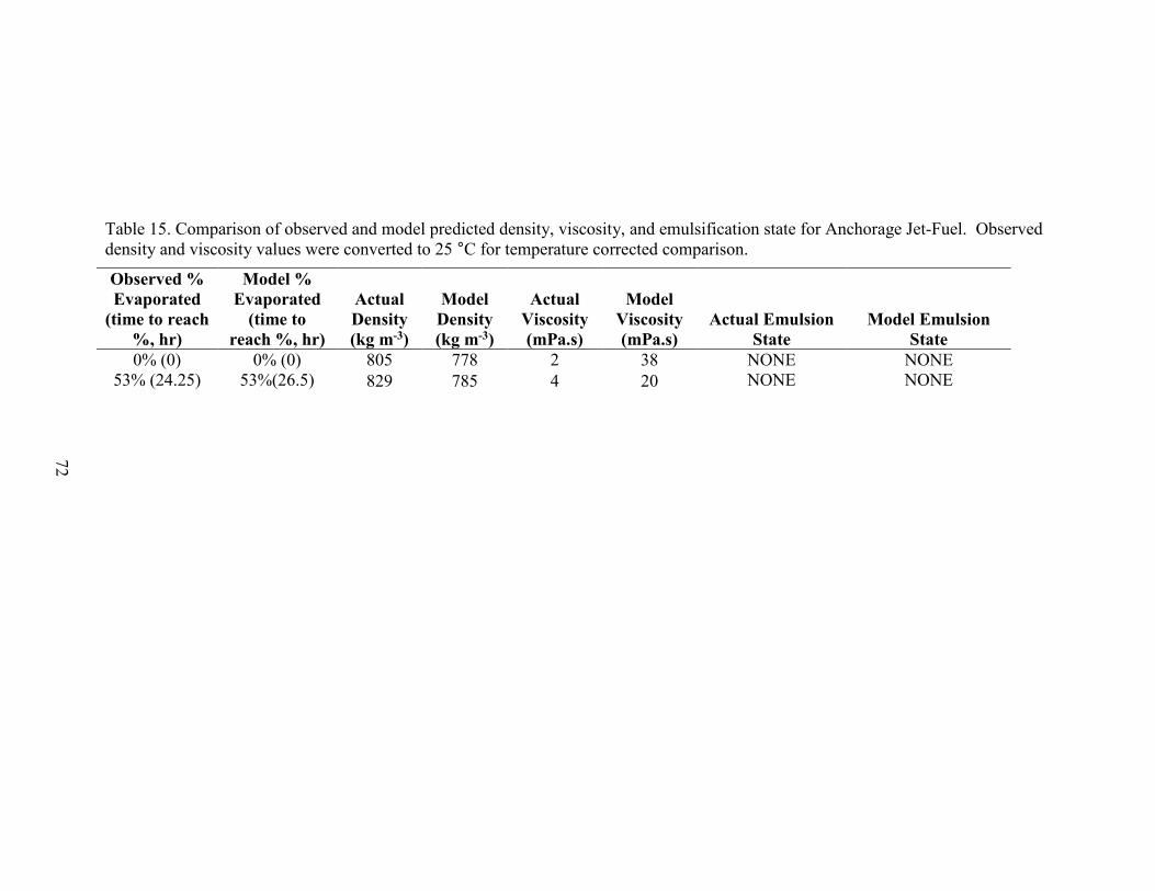
72

Table 15. Comparison of observed and model predicted density, viscosity, and emulsification state for Anchorage Jet-Fuel. Observed density and viscosity values were converted to 25 °C for temperature corrected comparison.

Observed %

Evaporated

(time to reach

%, hr)

Model %

Evaporated

(time to

reach %, hr)

Actual

Density

(kg m-3)

Model

Density

(kg m-3)

Actual

Viscosity

(mPa.s)

Model

Viscosity

(mPa.s)

Actual Emulsion

State

Model Emulsion

State

0% (0) 0% (0) 805 778 2 38 NONE NONE

53% (24.25) 53%(26.5) 829 785 4 20 NONE NONE

73

Figure 10: Comparison of laboratory predicted evaporation curve and model predicted evaporation during the first 48 hours for Arabian Light crude oil. Inset picture displays results for the first 6 hours.

74

Figure 11: Comparison of laboratory predicted evaporation curve and model predicted evaporation during the first 48 hours for Hondo crude oil. Inset picture displays results for the first 6 hours.

75

Figure 12: Comparison of laboratory predicted evaporation curve and model predicted evaporation during the first 48 hours for Santa Clara crude oil. Inset picture displays results for the first 6 hours.

76

Figure 13: Comparison of laboratory predicted evaporation curve and model predicted evaporation during the first 48 hours for Jet Fuel. Inset picture displays results for the first 6 hours.

77

CHAPTER 5

CONCLUSIONS

As an operational response model, the current oil spill modeling tools, with

simplified compositions and generic constituent class percentages for SARA contents,

appear to do a reasonable job at forecasting the fate and transport of crude oils.

Reasonable is not clearly defined in this industry as there are no industry-accepted

metrics for accuracy of oil spill trajectory forecasts (Fingas 2014). Ideally, analytical

results would be available to validate model predictions. During emergency response

operations this is rarely the main focus of effort and available data is typically

incomplete at best. Uncertainties in the underlying hydrographic and meteorological

inputs manifest themselves in inaccurate slick size and overall trajectory. Improper

weathering algorithms would amplify these errors.

The evaporation model developed and presented in this work does a reasonable

job at estimating the evaporation of fuels and crude oils when spilled and capturing the

onset of and method of emulsification, the two main goals of this work. The model is

able to capture the general trend of laboratory observations fairly well across a range

of fuel densities, and does a reasonable job at capturing the transition from non-

emulsified to emulsified oil. The simplified crude oil composition seems, based on the

limited comparison to observations presented within this work, to be a useful

representation of typical crude oils. This is significant considering that the complexity

of crude oil composition was reduced to a list of roughly 300 constituents, and

suggests that the compositional distribution from a very limited set of oils can be

78

extrapolated to a larger group of oils while still maintaining applicability. The mass-

weighted density calculation replicates empirical data well. The use of a simple film

model characterizes the evaporation of materials at the earliest stages of weathering

within an acceptable margin of error, providing a conservative estimate of the rate

weathering of materials and therefore erring on the side of caution. The noted

exception to this was the weathering of Arabian Light crude oil, which did not reach

the conditions for a stable emulsion in the model and therefore weathering proceeded

at a faster rate than observed.

There are several key areas where adjustments and improvements to the model

construct and execution could be made to improve the overall functionality of the

model for operational response. The viscosity estimation method is still sub-optimal

relative to the reported laboratory results. This is an issue because the calculation of

the stability factor used to determine the emulsification state requires a reasonable

estimate of viscosity. The friction viscosity method employed represents the current

state of the art for calculating crude oil viscosity (Quiñones-Cisneros et al. 2015),

however errors or omissions in the individual constituent viscosity calculations causes

in errors in the composite calculations. Although model run temperatures were kept to

25 °C when comparing model predictions to empirical data to avoid any issues that

may have arisen from using prescribed constant constituent viscosity values where no

fitting data were available, there are several sources of error that may have contributed

to the overall viscosity. When calculating the individual constituent contribution to

overall viscosity, compound-specific critical parameters are needed. When these data

are missing, as is the case for asphaltene, resin, and several of the higher molecular

79

weight saturate and aromatic constituents, they were derived from available data. This

derived data may contribute to the overall viscosity error, with a simpler formulation

providing a more defensible composite viscosity result.

If the availability of critical parameters was used as a criterion for inclusion

within the oil formulation, asphaltene and resin contributions to viscosity would be

excluded. These contributions are critical to the overall crude oil composition. As

characterization of asphaltenic and resinous materials advances through molecular

simulation and analytical improvements, current research trends suggest that these

broad categories can be divided up, themselves, into more discrete categories based on

molecular weight, solubility, and polarity (Li & Greenfield 2014). Generating sub-

classes for asphaltenes and resins and including their behavior in the model creates a

potential to better tune model results to empirical data, when available. This approach

was not attempted in the current work. The anticipated variability between crude oils

and within a single reservoir would result in a less generic approach than needed for

an operational response crude oil model.

The current model construct allows for addition of new constituents if and

when additional molecular information becomes available and/or is required, whether

for resolving sub-classes of asphaltenes and resins or adding defined constituents of

concern to the saturate and aromatic classes, The data can be added simply as a named

constituent within the oil constituent list with an assigned overall mass percentage in

the oil and added to the overall chemical database with minimal effort. When

viscosity needs to be better matched to known data in order to best replicate

environmental behavior, the current methodology to handle that would be to modify

80

the asphaltene and/or resin viscosity contribution to the overall oil until a reasonable

match to empirical physical properties was achieved by the prescribe oil composition.

It may also be useful to implement a hybrid method for determining viscosity by

implementing the Beal method for low viscosity fuels and friction theory approach for

higher viscosity fuels. This requires knowledge of the fuel viscosity prior to

modeling, something that may or may not be available before operation response

timelines have been exceeded. Lastly, the limits used to determine the oil emulsion

stability class could be tuned to accommodate errors in the viscosity while calculating

emulsion state.

The slick spreading algorithm, derived from fundamental principles and first

published by Fay in the 1970’s, has been documented (Lehr 2001) to be inaccurate for

certain conditions. There is little consensus, however, on the best approach to slick

spreading. In the current construct, the slick spreading algorithm seems to do a

reasonable job when weathering is progressing most quickly, as there were no

significant discrepancies within the first 5-10 hours of weathering for the cases

highlighted. This does not indicate that spreading approach is valid, but rather, that,

with its known errors, it does a reasonable job.

The model stops evaporation once a stable emulsion is reached, however there

are still significant viscosity changes that are observed within stable and meso-stable

emulsified oils. The viscosity changes currently implemented in the model are derived

from observations in (Fingas 2011) however this does not seem to adequately capture

the higher viscosity values for emulsified oils as observed in the model-to-data

comparisons for the four highlighted oils. A large part of the discrepancy is believed

81

to be the result of the non-Newtonian behavior of emulsified oils, likely resulting in an

observed viscosity that has a more complex relationship to the shear rate or shear rate

history. The friction viscosity approach was initially thought to be better suited to

incorporating these variations. Changes to the emulsified oil viscosity algorithms

would be very straightforward to implement within the modeling framework if

available.

The evaporation rate and viscosity calculations include temperature dependent

impacts on property calculations, however the temperature dependence of density is

not included. Not including temperature dependence would result in under-predicting

the bulk density at lower temperatures; it may impact the ability to predict the

emulsion state, and necessitate further adjustment to the stability ranges assigned to

each of the emulsion states.

From a response perspective, a reasonable model forecast should provide

information that allows for development and implementation of an effective response

effort that mitigates the impact of spilled oil. For shoreline spills, this is often not

possible due to the disparity between the fine scale of coastal transport processes and

the coarse scale of the underlying hydrographic forcing information. Interaction with

the shoreline alters the trajectory of spilled oil, and stranded oil exhibits tidally

influenced shoreline storage and re-suspension. For offshore spills, it is far more

likely that an oil spill forecast would provide a forecast with a smaller error in the

direction of oil transport as well as the size of the oil slick generated from a spill. If an

operational forecast has a 20% margin of error, it is typically considered reasonable.

82

A skilled forecaster typically qualifies this margin of error, and thus a quantitative

metric is still not available.

Model processing times suggest that the complexity of the crude oil

composition meets operational requirements to run a 3 day simulation and forecast

within 10 minutes. This varies as a function of the number of model parcels used in

the Lagrangian modeling framework employed within the system, but a 250 particles

as a benchmark is currently being implemented for operational use. The addition of

entrainment algorithms, dissolution, and more specific characterization of water

infiltration into the crude oil matrix as a function of emulsification state would be

expected to enhance the analytical modeling abilities, but add little to the operational

application of the model currently.

Finally, to best capture real world dynamics, the implementation of shoreline

interactions, including oil grounding and re-suspension from the shoreline, interaction

with varying shoreline type as well as inclusion of how shoreline materials dictate

overall oil stranding merits additional consideration to better represent oil fate and

transport in near-shore environments.

83

APPENDICES

84

Appendix A. Oil Composition for Saturate and Aromatic Classes as Mass Percentages of Total Aromatics and Saturates, Respectively.

Saturates

Butane: 4.4195×10

-4

Pentane: 2.9919×10

-4

,

Hexane: 4.1886×10

-4

,

Heptane: 2.9919×10

-4

,

Octane: 5.9837×10

-4,

Nonane: 1.43×10

-2,

Decane: 1.3×10

-2,

Undecane: 3.68×10

-2,

Dodecane: 2.9482×10

-2

,

Tridecane: 4.5399×10

-2,

2,6,10-Trimethyldodecane: 1.6155×10

-2

,

Tetradecane: 4.0108×10

-2,

2,6,10-Trimethyltridecane: 1.9400×10

-2,

Pentadecane: 4.6268×10

-2

,

Hexadecane: 4.0712×10

-2

,

Nor-pristane: 1.6670×10

-2

,

Heptadecane: 2.7627×10

-2

,

Pristane: 2.1971×10

-2,

Octadecane: 2.4275×10

-2,

Phytane: 1.6532×10

-2

,

Nonadecane: 3.3828×10

-2

,

Eicosane: 3.1988×10

-2,

Heneicosane: 3.1879×10

-2

,

Docosane: 2.5793×10

-2

,

Tricosane: 1.8736×10

-2

,

Tetracosane: 1.7980×10

-2

,

Pentacosane: 1.8356×10

-2

,

Hexacosane: 1.6722×10

-2

,

Heptacosane: 1.5797×10

-2,

Octacosane: 2.5148×10

-2,

Nonacosane: 1.5080×10

-2,

Triacontane: 1.3273×10

-2,

Hentriacontane: 1.2475×10

-2,

Dotriacontane: 2.7127×10

-2,

Tritriacontane: 1.4088×10

-2,

85

Tetratriacontane: 1.3928×10

-2,

Pentatriacontane: 1.3291×10

-2,

Hexatriacontane: 1.2914×10

-2,

Heptatriacontane: 1.3767×10

-2,

Octatriacontane: 9.5876×10

-3,

Nonatriacontane: 9.6136×10

-3,

Tetracontane: 9.0360×10

-3,

Isobutane: 9.5549×10

-4,

Isopentane: 1.3248×10

-3,

Isohexane: 1.2090×10

-3,

Neopentane: 2.6927×10

-4,

Neohexane: 6.7313×10

-4,

Neoheptane: 4.2813×10

-4,

2,3-Dimethylbutane: 3.9941×10

-4,

Triptan: 1.6156×10

-4,

3-Methylpentane: 2.1115×10

-3,

2,3-Dimethylpentane: 2.7734×10

-3,


-3,


-4,

2,2,3-Trimethylpentane: 1.1040×10

-4,


-4,


-4,

2-methyl-3-ethylpentane: 3.3333×10

-4,

2-Methylhexane: 4.8467×10

-3,

3-Methylhexane: 4.3350×10

-3,

2,2-Dimethylhexane: 1.7893×10

-4,


-4,


-4,


-4,


-4,

2,3,4-Trimethylhexane: 2.1003×10

-4,


-4,


-4,

3-Ethylhexane: 4.7862×10

-4,

2-Methylheptane: 1.3571×10

-3,


-3,


-3,

2,3-Dimethylheptane: 4.0390×10

-4,


-4,


-4,

4-Ethylheptane: 9.6935×10

-3,

86

2-Methyloctane: 1.0299×10

-2,


-3,


-3,

Cyclopentane: 4.2005×10

-3,

Methylcyclopentane: 5.3518×10

-3,

1,1-Dimethylcyclopentane: 2.7061×10

-3,

cis-1,3-Dimethylcyclopentane: 5.6546×10

-3,

trans-1,2-Dimethylcyclopentane: 9.2896×10

-3,

trans-1,3-Dimethylcyclopentane: 6.0988×10

-3,

1,1,2-Trimethylcyclopentane: 2.8677×10

-3,


-3,


-3,


-3,

Ethylcyclopentane: 3.1100×10

-3,

Isopropylcyclopentane: 1.7771×10

-3,

Cyclohexane: 1.3813×10

-2,

Methylcyclohexane: 2.2465×10

-2,

1,1-Dimethylcyclohexane: 6.0584×10

-3,

Heptene: 9.0473×10

-3,

Methyldecalin: 2.9081×10

-3,

2-Methyldecalin: 4.3621×10

-3,

Ethyldecalin: 1.8216×10

-3,

2,6-Dimethyldecalin: 1.8216×10

-3,

1,1,2-Trimethyldecalin: 1.7004×10

-3,

Butyldecalin: 6.2200×10

-4,

Isobutyldecalin: 6.2200×10

-4

Aromatics

Benzene: 4.0346×10

-2,

Toluene: 1.0929×10

-1,

Ethylbenzene: 2.3459×10

-2,

o-Xylene: 4.4320×10

-2,

m-Xylene: 6.0015×10

-2,

p-Xylene: 6.0015×10

-2,

Cumene: 6.6898×10

-3,

Propylbenzene: 1.0763×10

-2,

1-ethyl,3-methylbenzene: 2.8425×10

-2,

p-Ethyltoluene: 1.1955×10

-2,

1,3,5-Trimethylbenzene: 3.7366×10

-2,

1-ethyl,2-methylbenzene: 1.3088×10

-2,

Pseudocumene: 5.36575×10

-2,

87

1,2-Diethylbenzene: 4.288359×10

-3,

o-Propyltoluene: 6.9537×10

-3,

m-Propyltoluene: 1.3192×10

-2,

p-Propyltoluene: 5.3842×10

-3,

Butylbenzene: 5.1060×10

-3,

sec-butylBenzene: 5.1457×10

-3,

o-Cymene: 9.2782×10

-4,

m-Cymene: 6.4967×10

-3,

p-Cymene: 3.6159×10

-3,

p-Xylene,2-ethyl-: 6.4769×10

-3,

o-Xylene,4-ethyl-: 9.5762×10

-3,

m-Xylene,2-ethyl-: 2.0265×10

-3,

1-ethyl-2,4-dimethylbenzene: 6.8544×10

-3,


-3,


-3,

1,2,4,5-Tetramethylbenzene: 1.0073×10

-2,

Pentylbenzene: 9.9736×10

-4,

Naphthalene: 1.5914×10

-2,

1-Methylnaphthalene: 2.1457×10

-2,

2-Methylnaphthalene: 3.4172×10

-2,

1,2-Dimethylnaphthalene: 9.9339×10

-3,


-3,

2-Ethylnaphthalene: 9.9339×10

-3,


-3,

2,3,6-Trimethylnaphthalene: 2.9404×10

-2,

1-Butylnaphthalene: 1.3292×10

-2,

Fluorene: 3.0398×10

-3,

1-Methylfluorene: 6.2186×10

-3,

9-Ethylfluorene: 8.1259×10

-3,

Dibenzothiophene: 1.0371×10

-3,

1-Methyldibenzothiophene: 3.0199×10

-3,

2-Methylbenzothiophene: 1.2914×10

-3,

4-Methyldibenzothiophene: 1.2914×10

-3,

3-Methyldibenzo[b,d]thiophene: 1.2914×10

-3,

3-Ethyldibenzothiophene: 1.8378×10

-3,

4-Ethyldibenzothiophene: 1.8378×10

-3,

2,7-Dimethyldibenzothiophene: 1.8378×10

-3,

4,6-Dimethyldibenzothiophene: 1.8378×10

-3,

1,2,3-Trimethyldibenzothiophene: 1.9868×10

-3,

2,4,8-Trimethyldibenzothiophene: 1.9868×10

-3,

4-Ethyl-6-methyldibenzothiophene: 1.9868×10

-3,

88

3,4,6,7-tetramethyldibenzothiophene: 1.1921×10

-3,

4,6-Diethyldibenzothiophene: 1.1921×10

-3,

6-Ethyl,2,4-dimethyldibenzothiophene: 1.1921×10

-3,

Phenanthrene: 6.1789×10

-3,

1-Methylphenanthrene: 3.0199×10

-3,


-3,


-3,,


-3,

2-Methylanthracene: 3.0199×10

-3,

3,6-Dimethylphenanthrene: 4.0729×10

-3,

3-Ethylphenanthrene: 4.0729×10

-3,

2-Ethylanthracene: 4.0729×10

-3,,

1,9-Dimethylanthracene: 4.0729×10

-3,

1,2,8-Trimethylphenanthrene: 2.3047×10

-3,

9-Ethyl-10-methylphenanthrene: 2.3047×10

-3,

1-Propylphenanthrene: 2.3047×10

-3,

2,7,9-trimethylanthracene: 2.3047×10

-3,

9-Propylanthracene: 2.3047×10

-3,

2,4,5,7-Tetramethylphenanthrene: 9.2716×10

-4,

1,3,5,7-Tetramethylanthracene: 9.2716×10

-4,

9,10-Diethylphenanthrene: 9.2716×10

-4,

Retene: 9.2716×10

-4,

9-Butylphenanthrene: 9.2716×10

-4,

9-Butylanthracene: 9.2716×10

-4,

Fluoranthene: 9.1392×10

-2,

Pyrene: 3.5961×10

-4,

1-Methylpyrene: 2.3841×10

-3,

2,7-Dimethylpyrene: 1.2583×10

-3,

1-Ethylpyrene: 1.2583×10

-3,

4-Ethylpyrene: 1.2583×10

-3,

1,2,3-Trimethylpyrene: 1.0431×10

-3,

4-Ethyl,5-methylpyrene: 1.0431×10

-3,

Propylpyrene: 1.0431×10

-3,

4-Propylpyrene: 1.0431×10

-3,

4,5-Diethylpyrene: 7.4504×10

-4,

4-Ethyl,5,10-dimethylpyrene: 7.4504×10

-4,

1-Butylpyrene: 7.4504×10

-4,

1,2,3,4-Tetramethylfluoranthene: 7.4504×10

-4,

Benzo[a]anthracene: 2.9802×10

-4,

Chrysene: 1.0808×10

-3,

6-Methylchrysene: 2.5431×10

-3,

89

5,6-Dimethylchrysene: 3.0000×10

-3,

1,3,6-Trimethylchrysene: 5.9603×10

-4,

1-Ethyl,2-methylchrysene: 5.9603×10

-4,

6-Ethyl,5-methylchrysene: 5.9603×10

-4,

2,4,5-Trimethylchrysene: 5.9603×10

-4,

6-Propylchrysene: 5.9603×10

-4,

1,2,7,8-tetramethylchrysene: 7.2848×10

-3,

6,12-Diethylchrysene: 7.2848×10

-3,

6-Butylchrysene: 7.2848×10

-3,

Benzo[b]fluoranthene: 1.0967×10

-4,

Benzo[a]fluoranthene: 2.0066×10

-5,

Benzo[e]pyrene: 2.4040×10

-4,

Benzo[a]pyrene: 5.7418×10

-5,

Perylene: 2.2848×10

-5,

o-Phenylenepyrene: 1.7643×10

-5,

Dibenzo[a,h]anthracene: 4.0928×10

-5,

Benzo[g,h,i]perylene: 4.3908×10

-5,

Biphenyl: 3.6557×10

-3,

Dibenzofuran: 5.3643×10

-4,

Acenaphthylene: 1.5894×10

-4,

Acenaphthene: 4.5696×10

-4,

Indane: 1.3331×10

-3,

Benzo[b]fluorene: 2.3444×10

-4,

Thiophene: 3.6159×10

-4,

2-Methylthiophene: 1.0768×10

-3,

3-Methylthiophene: 1.6033×10

-3,

2-Ethylthiophene: 1.9113×10

-3,

Benzo[b]thiophene: 1.3907×10

-4

,

3-Methylbenzo[b]thiophene: 1.9868×10

-4

,


-4

,


-4

,

5-Ethylbenzo[b]thiophene: 1.8543×10

-4

,

3,5-Dimethylbenzo[b]thiophene: 1.8543×10

-4

,

2-Ethylbenzothiophene: 1.8543×10

-4

,

2-Propylbenzothiophene: 4.4371×10

-4

,

2,5,7-Trimethylbenzo(b)thiophene: 4.4371×10

-4

90

BIBLIOGRAPHY

Almeda, R. et al., 2013. Effects of Crude Oil Exposure on Bioaccumulation of

Polycyclic Aromatic Hydrocarbons and Survival of Adult and Larval Stages of

Gelatinous Zooplankton. PLoS ONE, 8(10).

Baylaucq, A. et al., 2006. Dynamic Viscosity Modeling of Methane + n- Decane and

Methane + Toluene Mixtures : Comparative Study of Some Representative

Models. , 6466(October 2015).

Canada, E., Environment Canada Oil Properties Database. Environment. Available at:

http://www.etc-cte.ec.gc.ca/databases/oilproperties/ [Accessed April 1, 2016].

Chang, S.E. et al., 2014. Consequences of oil spills: A review and framework for

informing planning. Ecology and Society, 19(2).

Deacon, E.L., 1977. Gas transfer to and across an air/water interface. Tellus, 29(4),

pp.363–374.

Dietrich, D.E. et al., 2014. Oil Spill Risk Management: Modeling Gulf of Mexico

Circulation and Oil Dispersal, Hoboken, NJ: Scrivener Publishing LLC.

Fay, J.A., 1969. The spread of oil slicks on calm sea. In Proceedings of a symposium

on the scientific and engineering aspects of oil pollution of the sea. pp. 53–63.

Fingas, M., 2014. Handbook of Oil Spill Science and Technology. In M. Fingas, ed.

Hoboken, NJ: John Wiley & Sons, Inc, p. 728.

Fingas, M., 2011. Models for Water-in-Oil Emulsion Formation, Available at:

http://dx.doi.org/10.1016/B978-1-85617-943-0.10010-3.

Fingas, M.F., 1999. the Evaporation of Oil Spills : Development and Implementation

of New Prediction Methodology. Intenational Oil Spill Conference, pp.281–287.

91

Available at:

http://www.ioscproceedings.org/toc/iosc/1999/1\nhttp://www.ioscproceedings.or

g/doi/pdf/10.7901/2169-3358-1999-1-

281\nhttp://www.ioscproceedings.org/doi/pdf/10.7901/2169-3358-1999-1-i.

Fingas, M.F., 2014. Water-in-oil emulsions: formation and prediction. Journal of

Petroleum Science Research, 3(1), p.38. Available at:

http://www.jpsr.org//PaperInfo.aspx?ID=10236.

Fuller, E., Schettler, P. & Giddings, J.C., 1966. A new method for prediction of binary

gas. Industrial and Engineering Chemistry, 58(5), pp.18–27.

Garrett, R.M. et al., 1998. Photooxidation of crude oils. Environmental Science and

Technology, 32(23), pp.3719–3723.

ITOPF, I.T.O.P.F., 2016. ITOPF. Available at: http://www.itopf.com/knowledge-

resources/documents-guides/fate-of-oil-spills/weathering/ [Accessed August 26,

2016].

Jones, J.C., 2012. Hydrocarbons - Physical Properties and their Relevance to

Utilisation, Available at: http://bookboon.com/en/textbooks/chemistry-chemical-

engineering/hydrocarbons.

Lehr, W.J., 2001. Review of modeling procedures for oil spill weathering behavior.

Advances in Ecological Sciences, 9, pp.51–90.

Leirvik, F. & Myrhaug, J.L., 2009. Sintef report: Weathering properties of the

Alvheim crude oils Kneler, Boa, Kameleon, and the Alvheim blend,

Li, D.D. & Greenfield, M.L., 2014. Chemical compositions of improved model asphalt

systems for molecular simulations. Fuel, 115, pp.347–356.

92

Liu, Y. & Kujawinski, E.B., 2015. Chemical composition and potential environmental

impacts of water-soluble polar crude oil components inferred from esi FT-ICR

MS. PLoS ONE, 10(9).

Manning, F.S. & Thompson, R.E., 1995. OILFIELD PROCESSING Volume Two:

Crude Oil Second., Tulsa: PennWell Publishing Company.

Mobil Research and Engineering, 1997. Petroleum Manufacturing Orientation

Course, Paulsboro, NJ.

Moreno, R. et al., 2013. Ten years after the prestige oil spill: seabird trophic ecology

as indicator of long-term effects on the coastal marine ecosystem. PloS one,

8(10), p.e77360. Available at:

http://www.pubmedcentral.nih.gov/articlerender.fcgi?artid=3793948&tool=pmce

ntrez&rendertype=abstract.

Nayar, K.G. et al., 2016. Thermophysical properties of seawater: A review and new

correlations that include pressure dependence. Desalination, 390, pp.1–24.

NOAA, 2012. Open Water Oil Identification Job Aid for Aerial Observation.

Available at:

http://response.restoration.noaa.gov/sites/default/files/OWJA_2012.pdf.

NOAA/ORA/ESRL PSD, NCEP Reanalysis Derived data provided by the

NOAA/OAR/ESRL PSD. , p.http://www.esrl.noaa.gov/psd/data/gridded/data.nce.

Available at: http://www.esrl.noaa.gov/psd/ [Accessed February 4, 2016].

Quiñones-cisneros, S.E. et al., 2008. Friction Theory Modeling of the Non-Newtonian

Viscosity of Crude Oils †. , 110(25), pp.799–804.

Quiñones-cisneros, S.E. et al., 2015. PVT Characterization and Viscosity Modeling

93

and Prediction of Crude Oils. , 6466(October).

Quiñones-Cisneros, S.E. et al., 2004. Viscosity modeling and prediction of reservoir

fluids: From natural gas to heavy oils. International Journal of Thermophysics,

25(5), pp.1353–1366.

Quiñones-Cisneros, S.E. & Deiters, U.K., 2006. Generalization of the friction theory

for viscosity modeling. Journal of Physical Chemistry B, 110, pp.12820–12834.

Quiñones-Cisneros, S.E., Zéberg-Mikkelsen, C.K. & Stenby, E.H., 2003. Friction

theory prediction of crude oil viscosity at reservoir conditions based on dead oil

properties. Fluid Phase Equilibria, 212, pp.233–243.

Quiñones-Cisneros, S.E., Zéberg-Mikkelsen, C.K. & Stenby, E.H., 2001a. One

parameter friction theory models for viscosity. Fluid Phase Equilibria, 178,

pp.1–16.

Quiñones-Cisneros, S.E., Zéberg-Mikkelsen, C.K. & Stenby, E.H., 2001b. The friction

theory for viscosity modeling: Extension to crude oil systems. Chemical

Engineering Science, 56, pp.7007–7015.

Reddy, C.M. et al., 2012. Composition and fate of gas and oil released to the water

column during the Deepwater Horizon oil spill. Proceedings of the National

Academy of Sciences , 109 (50 ), pp.20229–20234. Available at:

http://www.pnas.org/content/109/50/20229.abstract.

Ryerson, T.B. et al., 2012. Chemical data quantify Deepwater Horizon hydrocarbon

flow rate and environmental distribution. Proceedings of the National Academy

of Sciences, 109(50), pp.20246–20253.

Sanchez-Minero, F. et al., 2013. Predicting SARA composition of crude oil by means

94

of NMR. Fuel, 110, pp.318–321.

Sharqawy, M.H., Lienhard V, J.H. & Zubair, S.M., 2011. Erratum to Thermophysical

properties of seawater: A review of existing correlations and data. Desalination

and Water Treatment, 29(1-3), pp.355–355.

Sørheim, K.R., Altin, D. & Leirvik, F., 2011. Gjøa crude oil - Weathering propertires

related to oil spill response, and chemical and toxicological characterization of

WAF, Trondheim.

Thingstad, T. & Pengerud, B., 1983. The formation of “chocolate mousse” from

Statfjord crude oil and seawater. Marine Pollution Bulletin, 14(6), pp.214–216.

A Multi-Component Evaporation Model to Determine the Onset ...

Documents

Transcript of A Multi-Component Evaporation Model to Determine the Onset ...