
A Multi-asset Option Approximation for General Stochastic ...
43
Discussion Paper Number: ICM-2014-03 Discussion Paper A Multi-asset Option Approximation for General Stochastic Processes April 2014 Juan C Arismendi Z ICMA Centre, Henley Business School, University of Reading
Transcript of A Multi-asset Option Approximation for General Stochastic ...
Discussion Paper Number:
ICM-2014-03
Discussion Paper
A Multi-asset Option Approximation for General Stochastic Processes
April 2014
Juan C Arismendi Z ICMA Centre, Henley Business School, University of Reading
ii © Arismendi, April 2014
The aim of this discussion paper series is to
disseminate new research of academic
distinction. Papers are preliminary drafts,
circulated to stimulate discussion and critical
comment. Henley Business School is triple
accredited and home to over 100 academic
faculty, who undertake research in a wide range
of fields from ethics and finance to international
business and marketing.
www.icmacentre.ac.uk
© Arismendi, April 2014

A Multi-asset Option Approximation for General StochasticProcesses
J.C. Arismendi∗†
ICMA Centre - Henley Business School,University of Reading, Whiteknights, Reading RG6 6BA, UK
Phone/Fax: +44 (0) 118 378 8239
Dated: April 23, 2014
AbstractWe derived a model-free analytical approximation of the price of a multi-asset option defined over an
arbitrary multivariate process, applying a semi-parametric expansion of the unknown risk-neutral densitywith the moments. The analytical expansion termed as the Multivariate Generalised Edgeworth Expansion(MGEE) is an infinite series over the derivatives of the known continuous time density. The expected valueof the density expansion is calculated to approximate the option price. The expansion could be used to en-hance a Monte Carlo pricing methodology incorporating the information about moments of the risk-neutraldistribution. The numerical efficiency of the approximation is tested over a jump-diffusion density. Forthe known density, we tested the multivariate lognormal (MVLN), even though arbitrary densities could beused, and we provided its derivatives until the fourth-order. The MGEE relates two densities and isolatesthe effects of multivariate moments over the option prices. Results show that a calibrated approximationprovides a good fit when the difference between the moments of the risk-neutral density and the auxiliarydensity are small relative to the density function of the former, and the uncalibrated approximation hasimmediate implications over risk management and hedging theory. The possibility to select the auxiliarydensity provides an advantage over classical Gram–Charlier A, B and C series approximations. The densityapproximation and the methodology can be applied to other fields of finance like asset pricing, econometrics,and areas of statistical nature.
1 IntroductionThe distribution of the asset returns in equity markets is ‘fat-tailed’ and ‘skewed’ (Kraus and Litzenberger,1976; Harvey and Siddique, 2000). For this reason, a semi-parametric formula like that of Jarrow and Rudd(1982) profoundly impacted the literature. They approximated an arbitrary continuous risk-neutral density ofa univariate asset, using a Generalised Edgeworth Expansion (GEE) over a lognormal density. To obtain theoption price, they integrated the resulting approximated density under the risk-neutral measure. To calibratethe approximation, the GEE requires the empirical moments of the unknown density of the asset. By doingthis, not only the price is calculated, and the moments of the asset incorporated into the final formula, but alsothe effects of perturbations over the moments of the distribution on the option price can be easily observed.1
In this research, an approximate multi-asset option price is provided applying the Multivariate GeneralisedEdgeworth Expansion (MGEE) framework. In other words, we extend the results of Jarrow and Rudd (1982) tothe multivariate case. Our formula disentangles the impact of multivariate higher-order moments on the optionprices.2 It is the first time that a formula that disentangles the impact of multivariate higher-order moments on
∗Electronic address: [email protected].†The author wish to thank Chris Brooks and Marcel Prokopczuk for their valuable comments, and seminar participants at the
Mathematical Finance Days conference 2013, held at the HEC Montreal, and organised by the Institut de Finance Matématiquede Montrêal (IFM2), specially to Mario Ghossoub and Alexandre Roch, chair of the derivatives pricing session.
1As a result of the success of this model, it has been used in a large amount of empirical research, including Corrado and Su(1996), Bhandari and Das (2009) for options on portfolios, Lim et al. (2005) for a parametric option pricing model, Flamouris andGiamouridis (2002) for a semi-parametric model and Aït-Sahalia and Lo (1998) for a non-parametric model for density estimation.
2The option price formula is derived using a Fourier inversion method. Nevertheless, the method is applied for the large class ofcontinuous density functions with partial derivatives, resulting in a formula that is on the time domain, and there will be no needof a Fourier inversion method for pricing. In a paper by Níguezy and Perote (2008), a density expansion using the moments of the
1

2 J. C. ARISMENDI
option prices has been provided.3 The main advantage of our approximation is that it is for arbitrary processes;this means it can be used with discontinuous-time models originating not only from a Wiener diffusion, but alsofrom Levy processes like jump-diffusion.4 In the Jarrow and Rudd (1982) formula the value of the Europeanoption is equal to the Black and Scholes price plus corrections based on the difference of the moments of thelognormal distribution and the real market distribution. In this paper, the GEE is extended to the multivariatecase (MGEE), and then the Black and Scholes price is calculated using a Monte Carlo simulation, as there existsno equivalent closed-form Black and Scholes formula for the multivariate case. An analysis of multi-asset model-free option pricing methodologies compared with structural methodologies could be developed with the MGEE.Another benefit of our results is that the moments of the risk-neutral density of the assets could be obtainedseparately through empirical work and, if they are available, then the price of the option is straightforwardlyobtained using our formula. As a result, higher-order moment effects like the ones observed during marketcrashes can be easily modelled into the pricing or the hedging of the option.
The approximation provided allows us to calculate the moments of the distribution of the sum of lognormalsin a multivariate setting, and this can be considered an interesting result not only for finance, but in general.5In Ju (2002), an univariate approximation of the risk-neutral density is provided, using a Taylor expansion overa univariate lognormal density. Kristensen and Mele (2011) also provide an approximation with an applicationto asset pricing theory. This approximation is based on a Taylor expansion of a differential operator over thedivergence between the Black and Scholes model price and the real price. Consequently, the moments of thedistribution are not part of the option pricing formula, making it very difficult to understand how changes overthe distribution affect the final price.
Our approach for valuing multi-asset options using the multivariate risk-neutral density is novel, since allprevious models attempt to price multi-asset options with a function of univariate densities: Li et al. (2008) andLi et al. (2010) developed two new approximations, an original termed second-order boundary approximation,and an extension to the multivariate case of the Kirk (1996) formula for spread options termed the extended Kirkapproximation. Both approximations reduce the dimensions of the problem, from a multivariate integrationto a function of an univariate normal standard density. In Alexander and Venkatramanan (2011) the priceof a spread option is approximated as the price of the sum of two compound options, and that is extendedin Alexander and Venkatramanan (2012) for multi-asset options. The prices of the compound options werecalculated by Geske (1979) and by Carr (1988). The final formula will be a function of the product of univariatedensities. Working with the multivariate risk-neutral density requires additional notation from multivariatestatistics. Nevertheless, the main advantage for empirical research is a more realistic framework, and it providesnew tools for hedging and risk management.
The MGEE can be considered another important contribution of our research for other fields of applicationsuch as statistics. Although Perote (2004) and Del Brio et al. (2009) produced a Multivariate EdgeworthExpansion (MEE), this expansion is based on an approximation of the multivariate normal (MVN) distribution,with the complications of negative density values when the empirical density to fit is leptokurtic. We face thesame risk, but if we select an appropriate distribution with skewness and kurtosis more similar to the risk-neutraldensity, this problem is diminished.
The structure of this paper is as follows: Section 2 examines the use of the MGEE approximation for hedgingand risk management, and contains the definitions and the notation used. Section 3 describes the MGEE, andthe method used in finding an approximation for multi-asset options. Section 4 presents the multi-asset optionapproximation. We integrate the resulting density from the MGEE using a Monte Carlo method. In Section 5,a numerical example is presented, where the MGEE is used to price an option over a multivariate jump-diffusionprocess and introduce the possible extensions in the use of the MGEE as a tool for risk management. In Section6 we provide a calibration methodology. In Section 7 we present concluding remarks and further developmentswith some possible modifications to our approach.
distribution termed General Moments Expansion (GEM) is provided. This expansion generates only positive densities; however, itneeds an additional vector of parameters of the same dimension of the distribution dimension; these additional parameters have noeconomical significance.
3Schlögl (2013) provides an multi-asset option approximation using a multivariate Gram–Charlier A series expansion; however,there are assumptions over the risk-neutral density, and an additional methodology is needed to extract the moments inside theexpansion from the Hermite polynomials.
4Our results complement the results of Filipović et al. (2013), as we provide a thorough study of the higher-order momentseffect over option prices. In Knight and Satchell (2001) a Gram–Charlier expansion is derived for pricing options using the firstfour moments of a univariate risk-neutral distribution.
5Limpert et al. (2001) and Dufresne (2004) review the importance of the distribution of the sum of lognormals in finance, andin physical sciences in general.
2

A MULTI-ASSET OPTION APPROXIMATION 3
2 Hedging the risk-neutral densityA natural step for research on option pricing is the extension of all univariate models to the multivariate assetclass. There exist popular versions of multi-asset options, one of which is the basket option: given a vector ofweights ω = ω1, . . . , ωn, a strike price K, and a n-variate vector of assets S(t) = S1, . . . , Sn, the payoff ofa basket option is Π(S(t),ω,K) = [ω1S1(t) + · · ·+ ωnSn(t)−K]+. Rainbow, quanto, spread, Asian, and evenindex options can be regarded in the class of multi-asset options. In general, the payoff of multi-asset options canbe specified as a function of the assets: Π(S(t),H,K) = [H(S1(t), . . . , Sn(t),K)]+, where H(·) is a multivariatereal function. A special case of basket options is the spread option, which is highly traded on NYMEX. Thecompilation made by Carmona and Durrleman (2006) is a very extensive and complete examination of theprevious attempts and models that addressed the issue of pricing and hedging spread options. Numericalmethods like Monte Carlo, Binomial and Trinomial trees, and Fourier transforms had been used; however, allthese methods use an approximation of the univariate density of the sum of the assets.
The methodology used in this research calculates the option value approximating the risk-neutral densityusing the difference of its first four moments against moments of an auxiliary density. Let X,S be two univariaterandom variables, with densities fX and gS , respectively, and Π(S) a payoff function equal to Π(X), butchanging X by S. The most important attribute of the Jarrow and Rudd (1982) approximation is that it linksthe difference of the cumulants of two distributions with the price of the option:
C0(Π(X)) = C0(Π(S)) + 2nd order cumulants∂2gS∂S2
− 3rd order cumulants∂3gS∂S3
+ 4th order cumulants∂4gS∂S4
.
The intuition is that an increase of the volatility of the risk-neutral density will increase the price of the option,an increase in the skewness will reduce the price, and the increase of the kurtosis will again increase the price.In our approximation, the changes of the risk-neutral density over the price can then be measured using thismethodology. It is easier to estimate the moments of fX(t) by modelling risk-neutral asset prices as a multivariatevariable using option market prices, than estimating the moments of the risk-neutral payoff density function fΠ.It is assumed that the asset risk-neutral density fX(t) is unknown, but its moments are available. This densitycan be approximated using another known parametric density gS(t), from which we can calculate the moments.
In this section we examine the use of multivariate risk-neutral densities for option pricing and hedgingthrough some examples. We introduce some notation:
2.1 Model setupIn this section we define the arbitrary processes that can be approximated using a MGEE. Let X(t) =Xi(t) ∈ R+, t ≥ 0 , i ∈ 1, . . . , n be a general n-variate continuous stochastic process. This process is calledthe asset price process. Let Q be the n-variate risk-neutral probability measure. Denote by fX(t) the existentand unique density of X(t) under Q. We restrict X(t) to the class of processes where fX(t) is a continuousdensity function, and its partial derivatives (dfX(t)/dXi(t)) exist. Define the filtered probability space (Ω,F , Q),where F is the filtration generated by the sigma-algebra X : Ft = Xi(t), t ≥ 0.
Additionally, define the n-variate stochastic process S = Si(t) ∈ R+, t ≥ 0 , i ∈ 1, . . . , n, described by:
dSi(t) = µiSi(t)dt+ σiSi(t)dWi(t), (1)⟨dWi(t), dWj(t)⟩ = ρi,jdt,
where i, j ∈ 1, . . . , n, Wi(t) are Wiener processes under the risk-neutral measure Q, and µi, σi are the constantmean and the constant volatility of the variable Si(t), and ρi,j is the constant correlation between Si(t) andSj(t). The process S(t) will be used to approximate the asset price process X(t), and has a multivariatelognormal density function gS(t) under the risk-neutral measure Q (see Section 4.1). To simplify the optionpricing formula provided and its derivation, the risk-free interest rate r will be considered constant.
The gist of the model approximation is to use the properties of the well-known distribution gS(t) of thegeometric Brownian motion (GBM) process S(t), to fit the unknown distribution fX(t). In this sense we willhave:
fX(t) = H(gS(t)) + ε,
where H is a function with information about the moments of fX(t), and ε is a bounded error term. Denote byΠ(X(t)) a payoff function over the asset price. Then, the price of the European option Ct=0(Π(X(t))) is theexpected value of the discounted payoff under the risk-neutral measure:
C0(Π(X(t))) = exp(−rt)EQ0 [Π(X(t))] ,
3
4 J. C. ARISMENDI
and to calculate this expected value, we use H(gS(t)) instead of the unknown risk-neutral density fX(t):
EQ0 [Π(X(t))] = E
fX(t)0 [Π(X(t))] ≈ EgS(t)
0 [Π(S(t))] .
2.2 Multi-asset optionsThe value of an option can be calculated with the expected value of the risk-neutral density. In the case of abasket option, where the payoff is given by,
Π(X(t),ω,K) = [ω1X1(t) + · · ·+ ωnXn(t)−K]+. (2)
It is important to mention that there are two possible approaches for calculating the expected value. The firstapproach is to compute the option price with the univariate density function fΠ of the payoff Π(X(t),ω,K); thatis, a density function of the sum of the components
∑ni=1Xi(t). Then the expected value is found evaluating a
single integral over the univariate risk-neutral density of the payoff:
C0(Π(X(t)),ω,K) =
∫ ∞
0
Π(x(t))dFΠ, (3)
This is the dominant method used in the literature. An example is the basket option valuation of Margrabe(1978) and, more recently Ju (2002), Alexander and Venkatramanan (2012) and Li et al. (2010). In thesearticles, the density of the payoff function is usually modelled as a convolution of the sum of the densities oflognormal distributions.
The second approach is to integrate the payoff function over the assets’ multivariate risk-neutral densityfX(t), and this implies the need to compute a multivariate integral:
C0(Π(X(t)),ω,K) =
∫ ∞
0
. . .
∫ ∞
0
Π(x(t))dFX(t). (4)
The univariate density of the sum is usually more complex to define than the multivariate risk-neutral densityof the assets. For example, the probability density function (pdf ) of the sum of lognormals is unknown, whilethere exists a known pdf for the multivariate lognormal density. However, the integral region of (4) will be acomplex multivariate truncated region, while the integral region in (3) will be an easier univariate truncatedone. We use the second method. Although it is more demanding and complex in the number of integrals andthe region of integration, it will bring more information than using the first method.
2.3 Hedging and pricing with multivariate risk-neutral densityThe fundamental reason for using the second approach is to provide additional information to the trader,hedger or risk manager about the price of the option. The univariate density of the sum of lognormals hasturned out to be useful in the approximation of the option price, albeit it does not provide insights about themultivariate attributes of the risk-neutral density. Then, for hedging it is imperative to use the multivariatedensity. Nevertheless, it seems counter-intuitive to use a univariate density for pricing, and a multivariateversion for hedging. As an example, let us assume that a hedger uses a univariate sum of two lognormals tohedge an option:
Let Π(S(t),K) be the payoff function of a two-asset option, with price process Ct(Π(S(t),K)). Define theportfolio basket ΠP :
ΠP1(S(t),K) = C0(Π(S(t),K))−2∑
i=2
∆iSi(t), (5)
where the portfolio consists of one long position on C0(Π(S(t),K)), the two-asset option price process at timet = 0, and short positions ∆i, and the portfolio weights on each asset Si(t). Applying Itô’s lemma, this portfoliowill evolve by the process:
dΠP1(S(t),K) =
∂C0(Π(S(t),K))
∂t+
1
2
2∑i=1
2∑j=1
σiσjSi(t)Sj(t)∂2C0(Π(S(t),K))
∂Si(t)∂Sj(t)
dt+
2∑i=1
(∂C0(Π(S(t),K))
∂Si(t)−∆i
)dSi(t). (6)
4

A MULTI-ASSET OPTION APPROXIMATION 5
Setting ∆i =∂C0(Π(S(t),K))
∂Si(t), the portfolio in (5) will be risk-free:
ΠP1(S(t),K) = C0(Π(S(t),K))−2∑
i=2
∂C0(Π(S(t),K))
∂Si(t)Si(t), (7)
and (6) will lead to the multivariate Black and Scholes differential equation. Define a new asset, X(t) =S1(t) + S2(t). The distribution of this asset will be the distribution of the sum of two lognormals. Setting aportfolio as in (5), the risk-free portfolio will be:
ΠP1(X(t),K) = C0(Π(X(t),K))− ∂C0(Π(X(t),K))
∂X(t)X(t). (8)
As hedging in real-world applications can be applied only in discrete spaces of time, after a discrete jumpof time δt, δ > 0, the difference of the portfolio processes (7) and (8) will be determined only by the differencein the positions for each asset:
ϵ∆(t, t+ δt) = dΠP1(S(t+ δt),K)− dΠP1(X(t+ δt),K)
=2∑
i=1
(∂C0(Π(S(t),K))
∂Si(t)− ∂C0(Π(X(t),K))
∂X(t)
)dSi(t))
= ϵSi(t)dSi(t).
The difference ϵ∆(t, t+ δt) is the tracking error of using the portfolio ΠP1(X(t),K) with the univariate density.This error will be zero only if we use the appropriate distribution of the sum of lognormals to hedge, the onethat is still unknown in the literature at the time of the writing of this research.6
For the general case with n-assets, define σi = σ, i = 1, . . . , n as the volatility of the assets, and E[dSi(t)] =(r − 1
2σ2)dt as the expected drift of the assets. Assume that the difference ϵSi(t) = ϵc, i ∈ 1, . . . , n is constant
for t. The expected value of the tracking error over the time (0, t) will be:
E[ϵ∆(0, t)] = ϵc
(r − 1
2σ2
)dt,
and the variance:
V[ϵ∆(0, t)] = ϵ2c
(nσ +
n∑i=1
n∑i=1
ρi,jσ2
)dt.
The expected tracking error increases linearly with time, and a greater number of assets will increase the vari-ance, which could trigger a catastrophe.
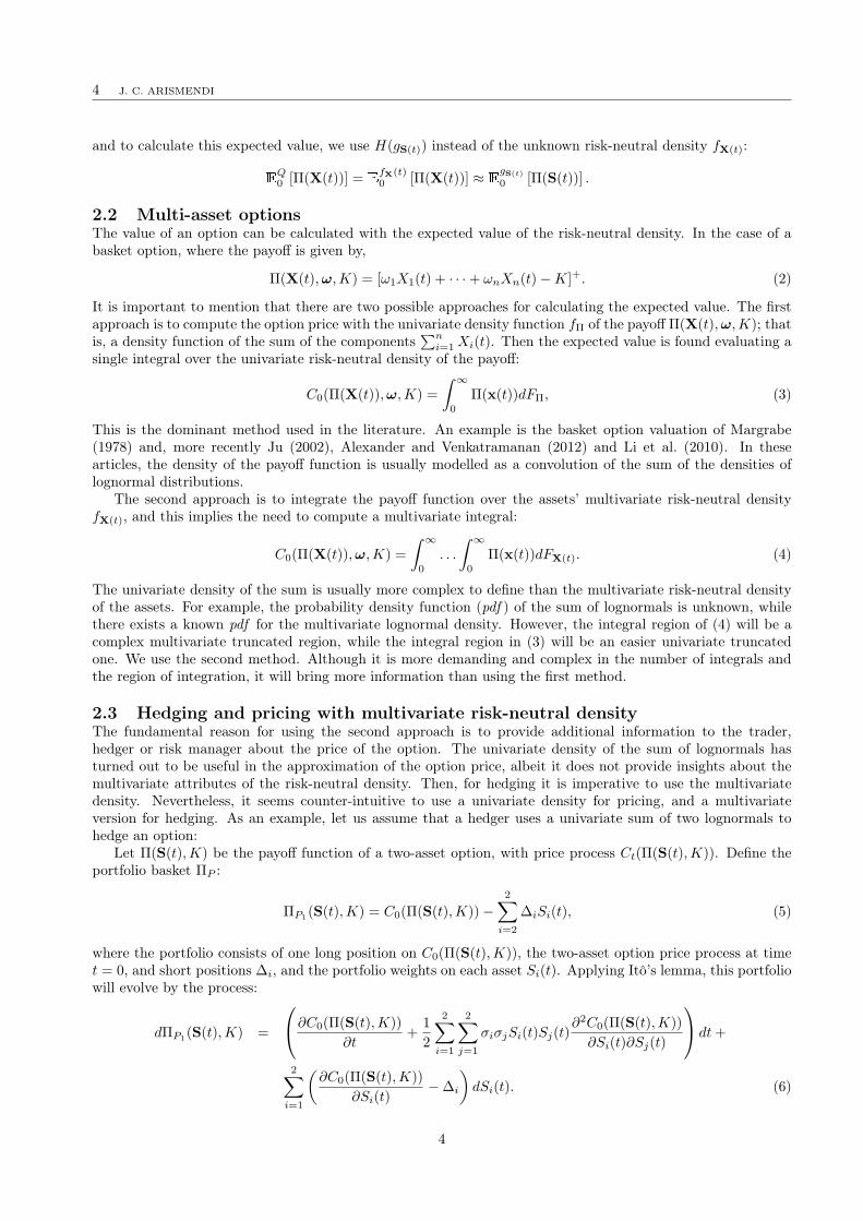
Example 1. Let S(t) be a bivariate GBM, with parameters S(0) = (30, 30), ρ = 0. Define a two-volatilities world,where the total volatility is equal to
√σ21 + 2σ1σ2ρ+ σ2
2 = 0.28284. Define a spread option: Π(S(t),K) =
[S1(t) + S2(t)−K]+ with K = 60. Denote by ∂C∂s1
≡ ∂C0(Π(S(t),K))∂S1(0)
, ∂C∂s2
≡ ∂C0(Π(S(t),K))∂S2(0)
the risk-neutral Delta
of the assets Si(t) at time t = 0, and ∂C∂s ≡ ∂C0(Π(S(t),K))
∂S(0) the Delta of the sum of assets S(t) = S1(t) + S2(t).We use two approaches for hedging: the first with portfolio (7), and the second with portfolio (8). In Figure1a, the profit and loss of the two portfolios in the two scenarios are plotted, each with changes on assets ofSi(t) = Si(0)± 0.1. The portfolio in (8) differs from the portfolio in (7) by ∼ 1%− 1.5% for different volatilityproportions (σ1/(σ1 + σ2)), and it will be equal only in the middle, when the volatility is equally distributed inboth assets. In Figure 1b, the values of Deltas ∂C
∂s1, ∂C∂s2
and ∂C∂s for different volatility proportions are plotted.
It is possible to observe that the difference in the Delta values is increased when the volatility is biased towardsone asset, with implications for the tracking error of Figure 1a.
The tracking error ϵ∆(t, t+ δt) is the result of an incorrect use of the sum of lognormal distributions of thepayoff function Π(S(t),K), due to the lack of a closed-form expression for its pdf. Therefore, using a multivariatedistribution yields an advantage for hedging and pricing.
6Even when the multivariate density is used for hedging, in a two-volatilities world, if we swap the volatility of the asset S1(t)with the volatility of the asset S2(t), the price of the option will remain the same, although the hedge positions need to be changed,a counter-intuitive signal for a risk manager.
5
6 J. C. ARISMENDI
0.25 0.3 0.35 0.4 0.45 0.5 0.55 0.6 0.65 0.7 0.750.18
0.19
0.2
0.21
0.22
0.23
0.24
0.25
0.26
0.27
Pro
fit &
Los
s
Proportion of Total Volatility of Asset 1 = σ1 /(σ
1 + σ
2)
Hedge: ∂ C/∂ s1,∂ C/∂ s
2,
Portfolio: s1−0.1, s
2+0.1
Hedge: ∂ C/∂ s,Portfolio: s
1−0.1, s
2+0.1
Hedge: ∂ C/∂ s,Portfolio: s
1+0.1, s
2−0.1
Hedge: ∂ C/∂ s1,∂ C/∂ s
2,
Portfolio: s1+0.1, s
2−0.1
(a) Profit and loss of hedged portfolios: two portfoliostimes two future scenarios in (s1, s2).
0.25 0.3 0.35 0.4 0.45 0.5 0.55 0.6 0.65 0.7 0.750.61
0.62
0.63
0.64
0.65
0.66
0.67
0.68
0.69
Proportion of Total Volatility of Asset 1 = σ1 /(σ
1 + σ
2)
Del
ta
∂ C/ ∂ s1
∂ C/ ∂ s2
∂ C/ ∂ s
(b) Values of ∂C∂s
, ∂C∂s1
, ∂C∂s2
for different proportions oftotal volatility assigned to s1.
Figure 1: Effects of hedging with univariate risk-neutral densities vs. multivariate risk-neutral densities.
Another important feature of the new approach is the use of the theory of multivariate truncated moments.Assume that S(t) is an univariate GBM, and Π(S(t),K) = [S(t)−K]+, with K a constant strike price. Applyingsimple probability and using the risk-neutral measure Q, the value of a European call option with maturity twill be:
C0(Π(S(t),K)) = exp(−rt)EQ0
[[S(t)−K, 0]
+]
= exp(−rt)PQ(S(t) ≥ K)(E
Q0 [S(t)|S(t) ≥ K]−K
). (9)
But, EQ0 [S(t)|S(t) ≥ K] is the first moment of the variable S(t) truncated at K, and PQ(S(t) ≥ K) is the
zero-th moment. Then, to value multi-asset European options we can use the theory of multivariate truncatedmoments. The results of Rosenbaum (1961), Tallis (1961), Finney (1963), and Arismendi (2013) could be usedfor this purpose.
3 The Multivariate Generalised Edgeworth Expansion (MGEE): thedistribution approximation
Before defining the distribution approximation we introduce tensor notation with the purpose of simplifyingthe final formula. Attempting to extend Jarrow and Rudd’s (1982) results to the multivariate case withoutthis notation would make the task intractable. We use the notation used by Kendall (1947) to provide generalresults. To simplify the notation, when the time index of an stochastic process is omitted we refer to the randomvariable at time t: X ≡ X(t).7
To define the tensor notation we use the summation convention as it is the appropriate notation for workingwith tensors. This notation is commonly used in physics and is attributed to Einstein. A tensor is a mathe-matical object similar to a multidimensional array. We use the brackets on the left-hand side to highlight theuse of this implicit summation convention:
Definition 3.1. Let a be a real valued vector of dimension m with components a1, . . . , am. A tensor productof X and a between p of their components is defined as:
a[l1] . . . a[lp]X[l1] . . . X[lp] ≡n∑
l1=1
· · ·n∑
lp=1
al1 . . . alpXl1 . . . Xlp ,
where l1, . . . , lp ∈ 1, . . . , n and the subscript [lp] represents a summation notation used to substitute the7The vector notation x(t) in lower-case refers to the variable of integration, then E(X) ≡
∫xdFX.
6

A MULTI-ASSET OPTION APPROXIMATION 7
summation symbol. The iterated tensor product x[l1,[l2,[l3,...,[lp]... ]]]a[l1] . . . a[lj ] is defined as:
X[l1,[l2,[l3,...,[lp]... ]]]a[l1] . . . a[lj ] ≡n∑
l1=1
Xl1al1 +n∑
l2=1
Xl1,l2al1,l2 + · · ·+n∑
lj=1
Xl1,...,ljal1,...,lj
.
Definition 3.2. Define the abbreviated integral operator as:∫ ∞
a1
. . .
∫ ∞
an
(· )dξ1 . . .dξn =(n)∫ ∞
ai
(· )dξ,
for i = 1, . . . , n where ξ is a vector with components (ξ1, . . . , ξn).The density approximation provided generalises the univariate results of Jarrow and Rudd (1982). Having
the same restrictions, the method can be applied only to the set of continuous distributions. More general dis-tributions can be included, but a more formal presentation using measure theory outside the scope of this paperwill be required. There have been previous attempts to approximate a distribution using other distributions:the multivariate Gram–Charlier and the multivariate Edgeworth expansion with the Edgeworth–Sargan densityof Perote (2004). However, in these cases the approximation is done over the multivariate normal distribution.This method has the inconvenience that only a limited set of distributions can be modelled, and heavy-taileddistributions especially can not be approximated with the MVN.
Definition 3.3. Let X have an absolutely continuous density function fX. We assume that fX is differentiableand that the cumulative distribution function FX exists. Let I = i1, . . . , ip be a vector of integer numbers,the p-order moment function of X is defined by,
mi1,...,ip(x) = mp,I(x) = E[Xi1 × · · · ×Xip
],
and these moments can be computed with the integral:
mI(x) =(n)∫ ∞
−∞
xi1 . . . xipfx
FXdx1 . . . dxn.
Another equivalent expression for moments is:
mα(x) = E[Xα11 Xα2
2 . . . Xαnn ], (10)
where α is a vector of integer numbers.
Assumption 3.1. The cumulants kl1,...,lj (x) of the unknown risk-neutral density fX are given.
Definition 3.4. Denote ψ(x, ξ) = E[exp
(ξ[l1]X[l1]
)]as the moment-generating function. The cumulant-
generating function (CGF) of x is defined as:
K(x, ξ) = logψ(x, ξ).
which is convergent for small ξ.
This function can be expanded into the infinite series:
logψ(x, ξ) = ξ[l1]k[l1](x) + ξ[l1]ξ[l2]k[l1,l2](x)/2! + ξ[l1]ξ[l2]ξ[l3]k[l1,l2,l3](x)/3! + . . . , (11)
=∞∑j=1
ξ[l1] . . . ξ[lj ]k[l1,...,l2](x)/j!,
which is convergent for small ξ where the terms kl1,...,lp(x) will be defined as the cumulants. The cumulantkl1(x) is the mean, kl1,l2(x) is the variance, kl1,l2,l3(x) is a measure of skewness and kl1,l2,l3,l4(x) is a measureof kurtosis. The expansion (11) can be used to find the values of kl1,...,lp(x).
7

8 J. C. ARISMENDI
Denote Ml1,...,lj as the difference of the moments of distributions fX, gS. In finance, the cumulants arecommonly used. The covariance matrix is a cumulant of second-order. The difference of the moments can beexpressed in terms of the difference of cumulants of X and S as:
M0 = 1,
Ml1 = kl1(x)− kl1(s),
Ml1,l2 = (kl1,l2(x)− kl1,l2(s)) +Ml1Ml2 ,
Ml1,l2,l3 = (kl1,l2,l3(x)− kl1,l2,l3(s)) + (Ml1 (kl2,l3(x)− kl2,l3(s)) +Ml2 (kl1,l3(x)− kl1,l3(s)) +
Ml3 (kl1,l2(x)− kl1,l2(s)) +Ml1Ml2Ml3 ,
Ml1,l2,l3,l4 = (kl1,l2,l3,l4(x)− kl1,l2,l3,l4(s)) + Ml1 (kl2,l3,l4(x)− kl2,l3,l4(s))(43) +
(kl1,l2(x)− kl1,l2(s)) (kl3,l4(x)− kl3,l4(s))S2(3)+
Ml1Ml2 (kl3,l4(x)− kl3,l4(s))(42) +Ml1Ml2Ml3Ml4 , (12)
where,
Ml1 (kl2,l3,l4(x)− kl2,l3,l4(s))(43) ≡ Ml1 (kl2,l3,l4(x)− kl2,l3,l4(s)) +Ml2 (kl1,l3,l4(x)− kl1,l3,l4(s)) +
Ml3 (kl2,l3,l4(x)− kl2,l3,l4(s)) +Ml3 (kl2,l3,l4(x)− kl2,l3,l4(s)) ,
is the sum over the partitions of four indices in two. The binomial(43
)notation represents the four possible
partitions of the set l1, l2, l3, l4 into two sets of one and three elements each.8 The notation,
(kl1,l2(x)− kl1,l2(s)) (kl3,l4(x)− kl3,l4(s))S2(3)≡ (kl1,l2(x)− kl1,l2(s)) (kl3,l4(x)− kl3,l4(s)) +
(kl1,l3(x)− kl1,l3(s)) (kl2,l4(x)− kl2,l4(s)) +
(kl1,l4(x)− kl1,l4(s)) (kl2,l3(x)− kl2,l3(s)) ,
represents the three different possible partitions of the set l1, l2, l3, l4 into two sets of two elements each. Thisnumber is equivalent to the number of partitions of the set of four elements into two sets, or the Stirling numberS2(3) = 23−1 − 1 = 3. Additional moments could be developed following combinatorics rules, and the work ofMcCullagh (1987) is a good reference for this purpose.
Proposition 3.1. Define X as an n-variate stochastic process with a multivariate continuous density functionfX. Define gS to be another multivariate continuous distribution defined over the random vector s. This densitywill be the approximate density. Denote ml1,...,lp(x) as the moment of order p of X and kl1,...,lp(x) the cumulantsof order p of X. Then, the density fX can be expressed in terms of the following expansion:
fX = gS +n−1∑j=1
M[l1,[l2,[...,[lj ]... ](−1)j
j!
∂j
∂s[l1] . . . ∂s[lj ]gS + ε(s, n),
where
ε(s, n) =1
2π
(n)∫ ∞
−∞exp(iξ′s)o(∥ξ∥n)dξ.
This expansion will be termed the Multivariate Generalised Edgeworth Expansion (MGEE). The tensor notationM[l1,[l2,[...,[lj ]... ] refers to:
M[l1,[...,[lj ]... ](−1)j
j!
∂j
∂s[l1] . . . ∂s[lj ]gS ≡
n∑l1=1
Ml1(−1)∂
∂sl1gS +
n∑l2=1
Ml1,l2
(1
2
)∂2
∂sl1∂sl2gS + · · ·+
n∑lj=1
Ml1,...,lj
(−1)j
j!
∂j
∂sl1 . . . ∂sljgS
.
8The binomial(42
)notation represents the possible partitions of the set l1, l2, l3, l4 into two sets of two elements each
8

A MULTI-ASSET OPTION APPROXIMATION 9
Proof. See Section A.1 of the appendix.
The MGEE approximation has been presented until the fourth-order moment. Continuous densities withtheir derivatives are candidates for the auxiliary distribution gs. Although the focus of this research is theapproximation of option prices using multivariate densities, the MGEE is useful for any application where thedensity fx is unknown, but the moments are available or they could be estimated.
4 Multi-asset option approximationThe result presented in the previous section will be used to approximate the risk-neutral distribution fX(t). Itis sufficiently general that it can be used for different distribution approximations. However, if we want to useit for basket option pricing we will need to provide additional approximations. The density approximation isused towards finding the value of a European multi-asset option. A general case is presented for the arbitrarycontinuous-time price processes X(t) described in Section 2.1:
Corollary 4.1. Denote the n-variate continuous-time stochastic price process X(t) with a unique continuousdensity function fX(t). Define S(t) as the multivariate lognormal process used to approximate X(t) and denoteby gS(t) the density function of S(t). Denote Π(S(t)) the payoff function, the value of an option Ct at time t = 0can be approximated as:
C0 (Π(x(t))) = exp(−rt)(n)∫ ∞
0
Π(s(t))dGS(t) +
exp(−rt)n−1∑j=1
M[l1,[...,[lj ]... ](−1)j
j!
(n)∫ ∞
0
Π(s(t))∂j
∂s[l1](t) . . . ∂s[lj ](t)gS(t)ds(t) + ε(Π(s(t)), n),
where ds(t) = ds1(t) . . . dsn(t) and,
ε(Π(s(t)), n) =1
2π
(n)∫ ∞
0
exp(iξ′s(t))o(∥ξ∥n)dξ.
Π(s) will be equal to Π(x) substituting the components xi by si.Proof. Using the risk-neutral pricing approach, the value of the option is:
C0(Π(x(t))) = exp(−rt)EQ0
[Π(X(t))
∣∣∣ F0
]= exp(−rt)
(n)∫ ∞
0
Π(x(t))dFX(t).
Then the result follows immediately from applying Proposition 3.1.
Denote:
C0,W(Π(x(t))) = exp(−rt)(n)∫ ∞
0
Π(s(t))dGs(t),
n−1∑j=1
C0,W,[l1,...,lj ](Π(x(t))) = exp(−rt)n−1∑j=1
M[l1,[...,[lj ]... ](−1)j
j!
(n)∫ ∞
0
Π(s(t))∂j
∂s[l1](t) . . . ∂s[lj ](t)gS(t)ds(t),
then the option price formula reveals three components:
C0(Π(x(t))) = C0,W(Π(x(t))) +n−1∑j=1
C0,W,[l1,...,lj ](Π(x(t))) + ε(Π(s(t)), n). (13)
The first part, C0,W(Π(x(t))), is the value of the option under a simple Black and Scholes world, of a multivariateWiener process with constant parameters, also known as geometric Brownian motion (GBM). In the univariatecase this part will be reduced to a Black and Scholes formula (Jarrow and Rudd, 1982). Given that therestill does not exist an equivalent Black and Scholes closed formula for the multivariate case, for numericalapplications, or to calibrate the model, an approximation of the first section is required. There are very good
9
10 J. C. ARISMENDI
approximations for the bivariate case (spread options), including Borovkova et al. (2007), Li et al. (2008) and,for the multivariate case, Li et al. (2010) and Alexander and Venkatramanan (2012). However, due to theimproved precision we use a Monte Carlo simulation method, integrating the payoff over the correspondinglognormal distribution.
The second part,∑n−1
j=1 C0,W,[l1,...,lj ](Π(x(t))), is the correction given by the MGEE, or the difference betweenthe moments of the asset distribution fX and the multivariate lognormal distribution gS times a partial derivativeof the lognormal distribution. In the univariate case this second part will be reduced to a lognormal density. Inthe multivariate case it can be demonstrated that reducing these partial derivatives to a multivariate lognormalis equivalent to finding the density of the sum of lognormal distributions, and this problem is still unsolved. Wederive expressions for the partial derivatives, and re-use the simulation paths of the first part of the formula tocalculate the integrals.
The third component of the formula, ε(Π(s(t)), n), is just the error of the approximation. We calculate somebounds for specific cases. These bounds will be determined in the section on the numerical efficiency of themodel, for the case of an option defined over jump-diffusion processes.
4.1 Value of C0,W(Π(x(t))): fitting multivariate Wiener processesThe general structure of the formula to value options over multivariate arbitrary processes was outlined in (13).Before we can find a formula for specific cases to provide numerical applications, we must find an approximationof:
C0,W(Π(x(t))) = exp(−rt)(n)∫ ∞
0
Π(s(t))dGS(t). (14)
Using as a payoff the definition of the basket option as in (2), the integral becomes,
(n)∫ ∞
0
[ω1s1(t) + · · ·+ ωnsn(t)−K]+dGS(t).
This integral can be rewritten as:
(n)∫[ω1s1(t)+···+ωnsn(t)−K]+
[ω1s1(t) + · · ·+ ωnsn(t)−K]gS(t)ds(t),
and this is just a function of the first moment of the multivariate density gS(t), truncated at the line ω1s1(t) +· · ·+ ωnsn(t) ≥ K. We need to find the density of gS(t). It is straightforward to demonstrate that the densityfunction gS(t) will be MVLN. Now, we find the parameters of gS(t):
Let the process S(t) be defined as in (1), with initial values S(0) = (S1(0), . . . , Sn(0)). Define the vectorlog(S(t)) = (log(S1(t)), . . . , log(Sn(t))). Applying Itô’s lemma to each component log(Si(t)), and solving thisdifferential equation we have:
log(Si(t)) = log(Si(0)) +
(r − 1
2σ2i
)t+ σiWi(t).
The distribution gS(t) will be n-variate lognormal with parameters:
µs =
log (S1(0)) +(r − 1
2σ21
)t
...log (Sn(0)) +
(r − 1
2σ2n
)t
Σs =
σ21t σ1σ2ρ1,2t · · ·
σ2σ1ρ1,2t σ22t · · ·
.... . .
. (15)
Define the vector log(S(t)) = (log(S1(t)), . . . , log(Sn(t))). Applying Itô’s lemma to each component log(Si(t)),and solving this differential equation we have:
log(Si(t)) = log(Si(0)) +
(r − 1
2σ2i
)dt+ σidWi(t).
Having found the density parameters of gS(t), the problem of solving the integral (14) reduces to finding thefirst moment of the multivariate lognormal with parameters (15), truncated at the semi-plane ω1S1(t) + · · · +
10

A MULTI-ASSET OPTION APPROXIMATION 11
ωnSn(t) ≥ K. Assume that we have a bivariate case with payoff Π(S(t)) = [S1(t) + S2(t)−K]+; the value
of such option will be EQ0
[(S1(t) + S2(t)−K)
+]. In Figure 2a we have an example of a bivariate lognormal
(BVLN) distribution truncated at the line [S1(t) + S2(t)−K]+, where the value of the option is the integral
under the surface. The equivalent problem in the univariate case is to calculate the first moment of the univariatelognormal truncated at S1(t) = 0.4: EQ
0
[(S1(t)−K)
+]
(see Figure 2b).
0 0.2 0.4 0.6 0.8 10
0.1
0.2
0.3
0.4
0.5
0.6
x
(a) Univariate lognormal density truncated atS1(t) = 0.4 with σ = 1, µ = 0.
(b) Bivariate lognormal density truncated atS1(t) + S2(t) = 0.4 with σ1, σ2 = 1, ρ = 0.8, µ = (0, 0).
Figure 2: The risk-neutral density of a GBM in the univariate an the bivariate case truncated at the payoff.
The multivariate integral is approximated using a Monte Carlo method:
C0,W(Π(x(t))) = exp(−rt)(n)∫
[ω1s1(t)+···+ωnsn(t)−K]+[ω1s1(t) + · · ·+ ωnsn(t)−K]gS(t)ds(t)
≈ exp(−rt) 1N
N∑p=1
(n∑
i=1
ωiSi(0)e(r− 1
2σ2i )t+σi
√tϕj
i −K
)+
,
where N is the number of path simulations, n the number of assets, and ϕpi is a multivariate normal standardvariable generated with correlations ρi1,i2 between assets Si1 , Si2 for the sample-path p.
4.2 Value of C0,W,[l1,...,lj ] (Π(x(t))): corrections of the price by moments of the risk-neutral distribution
For the second part of the formula, the integral will be approximated with a Monte Carlo simulation, althoughother methods like the Laplace inverse transform are suggested for future extensions of this work for cases oflow dimensionality.9 The sample-paths used to calculate the Wiener part C0,W(Π(x(t))) could be re-used tocalculate the integrals of C0,W,[l1,...,lj ] (Π(x(t))). We proceed to calculate the partial derivatives:
It turns out that the partial derivatives are functions of the density gS:
∂j
∂Sl1 . . . ∂Slj
gS(t) = gS(t)h(Sl1(t), . . . , Slj (t)
),
where h(Sl1(t), . . . , Slj (t)
)is a function of Sl1(t), . . . , Slj (t). In Section A.2 of the appendix there is a detailed
description of the form of the partial derivatives.For calculating C0,W,[l1,...,lj ] (Π(x(t))), the moments M[l1,[...,[lj ]... ] are given by the cumulants of the risk-
neutral density kl1,...,lj (x), and the cumulants kl1,...,lj (s) of the MLVN(µ,Σ) distribution are:
kl1,...,lj (s) = E [Sα11 Sα2
2 . . . Sαnn ] = exp
(1
2α′Σα+α′µ
), (16)
9As mentioned before, when the time index of the stochastic process is omitted we refer to the random variable at time t:s ≡ s(t).
11
12 J. C. ARISMENDI
where∑
i αi = j. The integrals are approximated using the Monte Carlo path simulations generated before forthe calculation of C0,W(Π(x(t))):
n−1∑j=1
C0,W,[l1,...,lj ](Π(x(t))) =
= exp(−rt)n−1∑j=1
M[l1,[...,[lj ]... ](−1)j
j!
(n)∫[ω1s1(t)+···+ωnsn(t)−K]+
[ω1s1(t) + · · ·+ ωnsn(t)−K]∂j
∂sl1 . . . ∂sljgS(t)ds(t)
≈ exp(−rt)
n−1∑j=1
M[l1,[...,[lj ]... ](−1)j
j!
1
N
N∑p=1
h(sl1(t), . . . , slj (t)
)( n∑i=1
ωisi(0)e(r− 1
2σ2i )t+σi
√tϕj
i −K
)+ .
4.3 Analysis of the correction term C0,W,[l1,...,lj ] (Π(x(t)))The term C0,W,[l1,...,lj ] (Π(x(t))) is developed further. With the intention of abbreviating the notation, the timeparameter is omitted, therefore s(t) ≡ (S1, . . . , Sn). By definition, the density gS is:
gS = (2π)−n/2 |Σs|−1/2
(n∏
i=1
S−1i
)exp
(−1
2(log(s)− µs)
′Σ−1
s (log(s)− µs)
), (17)
where log(s) = (log(S1), . . . , log(Sn)) and µs,Σs are the mean vector and covariance matrix defined in (15).The second part of the option approximation (13) up to the second-order is,
2∑j=1
C0,W,[l1,...,lj ](Π(s(t))) = exp(−rt)n∑
l1=1
Ml1(−1)(n)∫ ∞
0
Π(s(t))∂
∂Sl1
gS +
exp(−rt)n∑
l1=1
n∑l2=1
Ml1,l2
1
2
(n)∫ ∞
0
Π(s(t))∂2
∂Sl1∂Sl2
gS. (18)
Define by Σ−1s the inverse matrix of Σs:
Σ−1s =
ς1,1 ς1,2 · · ·ς2,1 ς2,2 · · ·...
. . .
. (19)
After the analysis of the correction terms of C0,W,[l1,...,lj ] (Π(x(t))) up to the second-order, developed in theSection A.3 of the appendix, we have that the first-order moment correction of (18) becomes:
exp(−rt)n∑
l1=1
Ml1(−1)(n)∫ ∞
0
Π(s(t))∂
∂Sl1
gS =
exp(−rt)
(n∑
l1=1
Ml1(−1)(Σ−1s,(l1,:)
µs − 1) exp(−µl1)(n)∫ ∞
0
Π(s(t))gS +
n∑l1=1
Ml1(−1) exp(−µl1)n∑
j=1
ςl1,j
(n)∫ ∞
0
log(Sj)Π(s(t))gS
).
The term log(Sj) = log(Sj(t)) is a log-contract, and it is an essential instrument to hedge variance swaps, andmoment swaps in general (see Neuberger, 1994; Demeterfi et al., 1999; Schoutens, 2005, for more details). Inthis case, the log-contract appears after applying the first-order partial derivative of the MVLN density, and itrepresents the sensitivity of the risk-neutral density to changes of Sl1(t), and it could be considered a kind of‘Delta’ of the risk-neutral density, with respect to future changes Sl1(t), and it is related to the classical ‘Delta’of changes with respect to the current stock price Sl1(0). The log-contract is essential for variance swaps, andsimilarly seems to be essential for the sensitivity to changes of Sl1(t).
12
A MULTI-ASSET OPTION APPROXIMATION 13
The second-order moment correction of (18) is (see Section A.3 of the appendix):
exp(−rt)n∑
l1=1
Ml1,l1
1
2
(n)∫ ∞
0
Π(s(t))∂2
∂S2l1
gS =
exp(−rt)
(n∑
l1=1
Ml1,l1
1
2exp(−2µl1)
(2− 3Σ−1
s,(l1,:)µs +
(Σ−1
s,(l1,:)µs
)2− ςl1,l1
) (n)∫ ∞
0
Π(s(t))gS +
n∑l1=1
Ml1,l1
1
2exp(−2µl1)
(3− 2Σ−1
s,(l1,:)µs
) n∑j=1
(ςl1,j)(n)∫ ∞
0
Π(s(t) log(Sj)gS +
n∑l1=1
Ml1,l1
1
2exp(−2µl1)
n∑j1=1
(ςl1,j1)2(n)∫ ∞
0
Π(s(t)) log(Sj1)2gS
),
and the second-order cross-moment correction is:
exp(−rt)n∑
l1=1
n∑l1=2
Ml1,l2
1
2
(n)∫ ∞
0
Π(s(t))∂2
∂S2l1
gS = exp(−rt)(n∑
l1=1
n∑l2=1
Ml1,l2
1
2exp(−µl1 − µl2)
(1− Σ−1
s,(l1,:)µs − Σ−1
s,(l2,:)µs +Σ−1
s,(l1,:)µsΣ
−1s,(l2,:)
µs − ςl1,l2
) (n)∫ ∞
0
Π(s(t))gS +
n∑l1=1
n∑l2=1
Ml1,l2
1
2exp(−µl1 − µl2)
n∑j=1
(ςj,l1
(1− Σ−1
s,(l2,:)µs
)+ ςl2,j
(1− Σ−1
s,(l1,:)µs
)) (n)∫ ∞
0
Π(s(t)) log(Sj)gS +
n∑l1=1
n∑l2=1
Ml1,l2
1
2exp(−µl1 − µl2)
n∑j1=1
n∑j2=1
(ςl1,j1ςl2,j2)(n)∫ ∞
0
Π(s(t)) log(Sj1) log(Sj2)gS
).
In this case we have calculated second-order sensitivities of the risk-neutral density to changes of S2l1(t), or a
‘Gamma’ equivalent of the risk-neutral density. The quadratic log-contract functions will produce quadraticvolatility terms or variance terms, essentials for calculating the sensitivity of the risk-neutral density to S2
l1(t).
We could extrapolate that the correction terms of higher-order consist of:
1. Functions of Wiener processes related to C0,W(Π(x(t))) with transformed MVLN densities,2. Sums of log-contracts times Wiener processes,3. Sums of cross log-contracts of higher-order times Wiener processes.
The option price approximation could be separated in three terms as in (13). The first term, C0,W(Π(x(t))), isan integral over a MVLN density as in the Black and Scholes (1973) world. For the second term, C0,W,[l1,...,lj ] (Π(x(t))),we analysed the expansion up to the second-order and we found that it could be expressed as an integral ofshifted MVLN densities times log-contracts and cross log-contracts. The expansions beyond the second-orderwill have a similar pattern given the nature of the MVLN density. This result could be used to hedge therisk-neutral density using the moments of higher-order, and further important theories could be developed fromthis result.
4.4 Analysis of the error term ε(Π(s(t)), n)We note that the error term of the MGEE is:
ε(Π(s(t)), n) =1
2π
(n)∫ ∞
0
exp(iξ′s(t))o(∥ξ∥n)dξ =
∞∑j=n
M[l1,[...,[lj ,[...]]... ](−1)j
j!
∂j
∂sl1 . . . ∂sljgS.
An analysis of this error term for arbitrary distributions is beyond the scope of this research. Numerical analysesin the univariate GEE for the lognormal case were done by Schleher (1977) and by Jarrow and Rudd (1982),and a deeper analysis of multivariate Edgeworth expansions was done by Skovgaard (1986). In our case, all thecumulants of the MLVN kl1,...,lj (s) exist (see Equation 16), and in case all cumulants of the risk-neutral density
13
14 J. C. ARISMENDI
Figure 3: Standard deviation of Monte Carlo integration algorithm for different number of simulated paths.
kl1,...,lj (x) exist the difference of cumulants Ml1,...,lj will be finite. Then, assuming,
limn→∞
M[l1,[...,[lj ,[...]]... ](−1)j
j!= 0.
it can be shown that,
limn→∞
sup ∥ε(Π(s(t)), n)∥ = 0,
noting by the result of previous section that,
limn→∞
∂n
∂sl1 . . . ∂slngS ≈ lim
n→∞
logn(Slj )
Snlj
gS = 0.
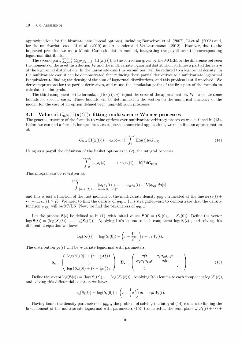
4.5 Performance of the MGEEThe MGEE requires an approximating distribution to fit the risk-neutral density. For pricing multi-asset optionslike spread or basket options, we will need to numerically integrate the expected payoff as it does not exist aclosed-form solution for these particular cases. Analytical approximations like Li et al. (2010) were tested forthe expansion of the correction terms in Section 4.3; however, results showed that the errors of the closed-form approximation were amplified when they were used with the MGEE, and precision is the most importantfeature of the expansion. A solution is to generate Monte Carlo sample-paths for pricing all the terms ofthe expansion. To select an appropriate number of simulations paths, we evaluated time and precision. Theprecision of the Monte Carlo algorithm increases at a rate of 1/
√N for any dimension, a favourable attribute
for high-dimension problems. In Figure 3 we plot the standard deviation of the Monte Carlo integration for theincreasing number of paths. Valuation of the integral was tested for pricing two different multi-asset optionswith jump-diffusion defined in Section 5.2. Valuations with up to 50,000,000 simulations were tested, findingthat 20,000,000 simulations would provide an approximate value with an error of approximately 0.3% for jump-diffusions with an intensity of λ = 1, and of approximately 10% for jump-diffusions with an intensity of λ = 10.In Table 1, we have the running time of the Monte Carlo algorithm, and the additional time consumed bythe successive MGEE. The second-order MGEE will consume only 30% more time than the MC algorithm,while the fourth-order MGEE will consume approximately eight times the time consumed by the Monte Carloalgorithm. Considering, that the option price precision could be improved in some cases by 20% (see Table 5),the MC option pricing with MGEE for cases when moments of the risk-neutral density are available would bea suitable decision.
14

A MULTI-ASSET OPTION APPROXIMATION 15
Table 1: Algorithm performance when moments of higher-order are included in the MGEE approximations ofjump-diffusion processes for different calibration methods. The columns MGEE2, MGEE3, and MGEE4 ofthe rows Uncalibrated, h2(σ), h3(σ), h4(σ) are the average running time of the option pricing and calibrationalgorithms for the 48 cases of Tables 9, 12, 13 and 14, respectively. The column ‘MC’ is the average runningtime of the Monte Carlo algorithm with 20,000,000 simulations.
Objective Function MC MGEE2 MGEE3 MGEE4Uncalibrated 581 172 591 3760h2(σ) = ∥Ml1,l2∥2 581 177 603 3750h3(σ) = ∥Ml1,l2∥2 + ∥Ml1,l2,l3∥2 581 183 631 3925h4(σ) = ∥Ml1,l2∥2 + ∥Ml1,l2,l3∥2 + ∥Ml1,l2,l3,l4∥2 581 185 652 4210
4.6 Empirical motivation of moments differenceThe partial derivatives and the cumulants’ corrections CW,[l1,...,lj ] in (13) have an economic sense. Denote thethree correction terms:
Mc,2 = M[l1,[l2]](−1)2
2!
∂2
∂sl1∂sl2gS(t), (Second) ,
Mc,3 = M[l1,[l2,[l3]]](−1)3
3!
∂j
∂sl1∂sl2∂sl3gS(t)/gS(t), (Third) ,
Mc,4 = M[l1,[l2,[l3,[l4]]]](−1)4
4!
∂4
∂sl1∂sl2∂sl3∂sl4gS(t)/gS(t), (Fourth) .
The value Mc,2 represents the density variance correction. If the variance of fX(t) is greater than the varianceof gS(t), the option price premium of the second cumulant is positive. Volatility has a positive premium. Thevalue Mc,3 is the density skewness correction. If the skewness of fX(t) is greater than the skewness of gS(t),the option premium is negative; skewness is transmitted into the option price as a negative correction. Thevalue Mc,2 is the kurtosis correction. If the kurtosis of fX(t) is greater than the kurtosis of gS(t), the optionpremium is positive; kurtosis is transmitted into the option price as a positive correction. All these relationsare consistent with Jarrow and Rudd’s (1982) results, except for the skewness correction, which differs becausewe have included the (−1)j
j! term. In Rubinstein (1998) the relationship between the univariate moments ofhigher-order and the prices of options are modelled in binomial trees. This research is useful as an extensionfor our work.
Figures 4a, 4b and 4c plot the moment corrections for two examples: a bivariate jump-diffusion processdefined in Section 4.7 with symmetrical volatilities σ1 = σ2 = 0.2, and a second with asymmetrical volatilitiesσ1 = 0.1, σ2 = 0.26458. Figure 4 shows that options where the difference of volatilities between the assets arehigher will have a greater impact in all moments’ differences Ml1,...,lj , li ∈ 1, . . . , 4. Figure 4 also displaysimportant information on the partial derivatives that could be used for sensitivity analysis in changes of therisk-neutral measures. Figure 4 shows the second, third and fourth cumulant differences total corrections (thesum of the cross-moments of the n-th-order correction). The second cumulant difference correction has oneinflection point near the at-the-money (ATM) price, the third cumulant difference correction has two inflectionpoints, one in-the-money (ITM) and the other out-of-the-money (OTM), and the fourth cumulant differencecorrection has three inflection points in ITM, ATM and OTM prices. This is consistent with the results ofJarrow and Rudd (1982). Figure 4 shows two cases: one with the components of volatility equal (σi − 0.2) in astraight line, and other where the component volatilities are different in a dashed-dot line. When the univariatedensity of the payoff is considered, the total volatility in both cases is equal, but when we consider a multivariatedensity a greater difference in the component volatilities will be transmitted as greater corrections in the priceof the option by the moments.
4.7 Analysis of the density values of the MGEE approximationThe selection of the MVLN as an auxiliary density comes as a result of two important attributes: it is thedensity on which the GBM process converges, the one which is widely used in the industry and is still thereference for option pricing in academia, and it possesses heavy tails.
The second attribute is of great importance when we need to validate that the resulting density approximationis in fact a density. The main problem that is faced using the MGEE to approximate a pdf is the possibility of
15

16 J. C. ARISMENDI
40 50 60 70 80 90 1000
0.02
0.04
0.06
0.08
0.1
0.12
0.14
Mc,
2
Strike
σ
1 = σ
2 = 0.2
σ1=0.1,σ
2=0.26458
(a) Second cumulant difference total correction.
40 50 60 70 80 90 100−0.06
−0.04
−0.02
0
0.02
0.04
Strike
Mc,
3
σ
1 = σ
2 = 0.2
σ1=0.1,σ
2=0.26458
(b) Third cumulant difference total correction.
40 50 60 70 80 90 100−0.06
−0.04
−0.02
0
0.02
0.04
Strike
Mc,
4
σ
1 = σ
2 = 0.2
σ1=0.1,σ
2=0.26458
Deep In−The−Money Out−of−the−money
At−The−Money Mean = (s
1(0)+s
2(0))ert
(c) Fourth cumulant difference total correction.
Figure 4: Second-, third- and fourth-order corrections with the partial derivatives of the MGEE approximationof two bivariate jump-diffusion processes. Both processes have λ = 0.5, νi = 0.1, δi = 0, ρi,j = 0, r = 0.05, t =0.25, Si(0) = 30, i, j ∈ 1, 2. The solid line is the total moment correction of the first process with σ1 = σ2 = 0.2,and the dash-dot line is the second process with σ1 = 0.1, σ2 = 0.26458.
16

A MULTI-ASSET OPTION APPROXIMATION 17
negative values in certain domains of the function approximation. The MGEE is a polynomial expansion overthe auxiliary density, where the parameters of the polynomial are M[l1,[...,[lj ]... ]
(−1)j
j! and ∂j
∂sl1 ...∂sljgS(t)/gS(t).
If the multiplication of these parameters is negative enough to outweigh the positive part of the function, theresulting MGEE function approximation will be negative.
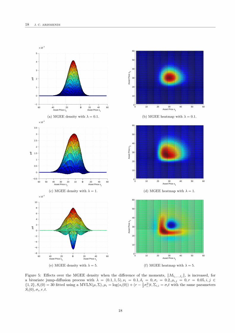
Let us consider the bivariate density of a jump-diffusion process with the parameters outlined in Example1 of Section 2.3. Now iterate over different jump intensities λ = 0.1, 1, 10. Increasing the intensity of thejumps will increase the higher-order moments, therefore the skewness and the kurtosis and M[l1,[...,[lj ]... ] will behigher. Figures 5a–5f plot the MGEE produce over a MVLN bivariate density to fit the desired moments. Inthe extreme cases of λ = 1 and λ = 5,10 the resulting MGEE density has negative values.
To overcome this problem, the selection of an auxiliary function with heavy tails will be a determiningfactor in the success of the application of the method. A calibration methodology to decrease the values ofM[l1,[...,[lj ]... ] will be developed in Section 6.
Example 2. The jump-diffusion process parameters for the numerical example are λ = 0.5, ν = 0.1, δ =0, S1(0) = S2(0) = 30, r = 0.05, t = 1. Two volatility scenarios are generated:11
1. In the first scenario, the risk-neutral density denoted by f1,X(t) has equal diffusion volatility for bothassets, σ1 = σ2 = 0.2,
√σ21 + σ2
2 = 0.2828.2. In the second scenario, the risk-neutral density denoted by f2,X(t) has different diffusion volatility, σ1 =
0.1, σ2 = 0.26458,√σ21 + σ2
2 = 0.2828.The auxiliary densities used by the MGEE are denoted by g1,S(t), g2,S(t). They have MVLN(µ1,Σ1), andMVLN(µ2,Σ2) distributions, and the same parameters Si(0), r, t of f1,X(t) and f2,X(t), respectively for µ1,µ2,Σ1,Σ2
as in (15). The value of a basket option with payoff Π(S(t)) = (S1(t) + S2(t)−K)+ with K = 60, is calculated
using a Monte Carlo simulation as described in Section 4.In Table 2, option prices derived from the application of the MGEE approximation with different levels of
moments are exhibited. The J-D Price column is the Monte Carlo option price of the contract with a jump-diffusion process, with 20,000,000 sample-path simulations. The Wiener column represents the option pricewithout jump-diffusion. Subsequent columns MGEE2, MGEE3, and MGEE4 are the option prices approximatedincluding the second-, third- and fourth-order cumulant corrections in the polynomial expansion. The %pdfcolumn is the percentage of the simulated sample-paths that when the MGEE is applied generate a positivedensity function, and the asterisk denotes the best approximation. By arbitrage arguments, the first cumulantsof f1,X(t) and g2,S(t) are equal, as in the case of f2,X(t) and g2,S(t).
Let us assume the current market risk-neutral density is f1,X(t) and the next time available for hedging isf2,X(t). Remember that the rebalancing of the portfolio for hedging in real applications is possible only on afinite number of times. The amount of premium for the option price is symmetrical in case the volatility issymmetrical; However, the premium shifts towards the second asset for f2,X(t). This is expected as the premiumvalues the difference f2,X(t) − g2,S(t). The reduction of the asset’s volatility σ2 from 0.2 to 0.1 is reflected as anincrease in the cumulant’s difference of 0.158, and this represents an 0.01 (0.19%) positive premium in the optionprice. If we use the univariate density of the sum of lognormals, as in Jarrow and Rudd (1982), an increase ofthe second- and fourth-order cumulants is reflected as a positive premium, while a decrease in the third-ordercumulant is considered as a negative premium. In the multivariate case the cross-cumulants cause an additionaleffect. Although the fourth cumulant differences of f2,X(t)−g2,S(t) are positive, the asymmetry generates a totalnegative premium of −0.0586 or −1.14%. A risk manager can use this information to evaluate the price impactwhen the risk-neutral density cumulants evolve over the time. To measure if there is any negative section ofthe MGEE density function, we simulate asset prices (S1(t), S2(t)) over the function domain, and calculate theassociated density function. After 20, 000, 000 paths simulations, in both approximations there were no negativedensity points found.
10Das and Uppal (2004) found through empirical study that λ in high-beta emerging markets is lower than 0.1.11In a complete market there exist only one risk-neutral density. However, we could be interested in examining the differences
between the risk-neutral densities of two different markets; for example, the risk-neutral density of a stock with the risk-neutraldensity of a commodity.
17
18 J. C. ARISMENDI
0 20 40 600204060−1
0
1
2
3
4
5
x 10−3
Asset Price s1
Asset Price s2
(a) MGEE density with λ = 0.1.
0 10 20 30 40 50 600
10
20
30
40
50
60
Asset Price s1
Ass
et P
rice
s 2
(b) MGEE heatmap with λ = 0.1.
0 20 40 600102030405060−0.5
0
0.5
1
1.5
2
2.5
3
3.5
x 10−3
Asset Price s1
Asset Price s2
(c) MGEE density with λ = 1.
0 10 20 30 40 50 600
10
20
30
40
50
60
Asset Price s1
Ass
et P
rice
s 2
(d) MGEE heatmap with λ = 1.
0 20 40 600204060−8
−6
−4
−2
0
2
4
6
8
10
x 10−3
Asset Price s1
Asset Price s2
(e) MGEE density with λ = 5.
0 10 20 30 40 50 600
10
20
30
40
50
60
Asset Price s1
Ass
et P
rice
s 2
(f) MGEE heatmap with λ = 5.
Figure 5: Effects over the MGEE density when the difference of the moments, ∥Ml1,...,lj∥, is increased, fora bivariate jump-diffusion process with λ = (0.1, 1, 5), νi = 0.1, δi = 0, σi = 0.2, ρi,j = 0, r = 0.05, i, j ∈1, 2, Si(0) = 30 fitted using a MVLN(µ,Σ), µi = log(si(0)) + (r − 1
2σ2i )t,Σi,i = σit with the same parameters
Si(0), σi, r, t.
18

A MULTI-ASSET OPTION APPROXIMATION 19
Table 2: Option prices of a basket with payoff Π(S(t)) = (S1(t) + S2(t)−K)+ when S1(t) and S2(t) are jump-
diffusion processes with common parameters λ = 0.5, ν = 0.1, δ = 0, S1(0) = S2(0) = 30 and the basket hasparameters r = 0.05, t = 1. We have two examples, one where the volatility is σf1,x(t)
= (0.2, 0.2) and otherwhere the volatility is σf2,x(t)
= (0.1, 0.26458) with risk-neutral densities f1,x(t) and f2,x(t), respectively. Theoption prices were approximated applying a MGEE over the auxiliary gi,s(t) MVLN densities (i = 1, 2) withoutany calibration of the density parameters.
J-D Price MC Wiener MGEE2 MGEE3 MGEE4 %pdff1,x(t),g1,s(t) 5.1668 4.9780 5.2113 5.2014 5.1685∗ 1.00f2,x(t),g2,s(t) 5.1141 4.9292 5.1761 5.1714 5.1127∗ 1.00
Table 3: Option prices of a basket with payoff Π(S(t)) = (S1(t) + S2(t)−K)+ when S1(t) and S2(t) are jump-
diffusion processes with common parameters λ = 0.5, ν = 0.1, δ = 0, S1(0) = S2(0) = 30 and the basket hasparameters r = 0.05, t = 1. We have two examples, one where the volatility is σf1,x(t)
= (0.2, 0.2) and otherwhere the volatility is σf2,x(t)
= (0.1, 0.26458) with risk-neutral densities f1,x(t) and f2,x(t), respectively. Theoption prices were approximated applying a MGEE over the auxiliary gi,s(t) MVLN densities (i = 1, 2) withoutany calibration of the density parameters.
J-D Price MC Wiener MGEE2 MGEE3 MGEE4 %pdff1,X(t),g1,S(t) 5.1668 4.9778 5.2145 5.2002 5.1505∗ 0.9999f2,X(t),g2,S(t) 5.1141 4.9184 5.1643 5.1621 5.0802∗ 0.9505
20 40 60 80 100 120−1
0
1
2
3
4
5x 10
−3
‖s1 + . . . + s5‖
(a) Density.
26 26.5 27 27.5 28 28.5 29−2
0
2
4
6
8
10
12
14x 10
−5
‖s1 + . . . + s5‖
(b) Negative density region in red.
Figure 6: Norm projection of the MGEE density of ∥(S1(t), S2(t))∥ when a jump-diffusion process with λ =0.5, ν = 0.1, δ = 0, σ1 = σ2 = 0.2,
√σ21 + σ2
2 = 0.2828, S1(0) = S2(0) = 30, r = 0.05, t = 1 is fitted (99.99%positive function).
5 Numerical analysis of multi-asset option pricing: methodscomparison
Consider that we are in a jump-diffusion risk-neutral world as in Merton (1976), but an asset manager doesnot acknowledge the presence of jumps, and actually he prices the options in the market considering only theWiener diffusions (GBM). The misspricing will be related to the size of volatility and the drift of the jumps,but let us assume both are unknown for the asset manager. In this section we developed a set of numericalexamples to test the benefits of measuring risk-neutral moments and using a MGEE, against using classicalmulti-asset options that do not incorporate this information. The analytic approximations of Li et al. (2010)and Alexander and Venkatramanan (2012) were developed and used to compare with the results of the MGEE,additionally to the results of plain vanilla Monte Carlo methodology. In Section 6, we will improve this testincorporating the risk-neutral moments information for all four different methodologies.
19

20 J. C. ARISMENDI
5.1 Multivariate Merton’s jump-diffusionTo measure the option pricing corrections with a practical example, we select as the candidate for the risk-neutral density to be approximated fX(t), the density on which a jump-diffusion (J-D) process of Merton (1976)converges. This process will also be used to measure the numerical efficiency of the MGEE option pricingapproximation in the Section 6. We extend the definition of Merton processes to the multivariate case:
Definition 5.1. Denote the multi-asset jump-diffusion (MJ-D) to the n-variate stochastic process X = Xi(t) ∈R
+, t ≥ 0, i ∈ 1, . . . , n, described by:
dSi(t) = µiSi(t)dt+ σixi(t)dWi(t) + (Ji(t)− 1)dPi(λ),
where Wi(t) are Wiener processes, Pi(λ) is a Poisson process with intensity parameter λ, and (Ji(t) − 1)represents the jump-size. The jump size has a normal distribution: Ji(t) ∼ ϕ
(δ, ν2
). We assume that the
jump’s size and the jump’s occurrence are independent, therefore uncorrelated between,
⟨Ji(t), Jj(t)⟩ = ⟨dPi(t), dPj(t)⟩ = 0,
with i, j ∈ 1, . . . , n, i = j, likewise the Wiener processes and the jumps:
⟨dWi(t), dPj(t)⟩ = ⟨dPi(t) = Jj(t)⟩ = 0.
On average, the MJ-D will be similar to a GBM diffusion:
dSi(t) = µiSi(t)dt+ σiSi(t)dWi(t),
but every λ times it jumps Ji(t)− 1, generating the change in the asset i:
dSi(t) = µiSi(t)dt+ σiSi(t)dWi(t) + (Ji(t)− 1).
For this process to be a martingale, the drift needs to be extracted:
dXi(t) =
(r − 1
2σ2i − b
)Xi(t)dt+ σiXi(t)dWi(t) + (Ji(t)− 1)dPi(λ),
where r is the constant risk-free interest rate and b is the adjustment due to the jump process. Merton foundthat, if the jumps are i.i.d., the price process will be lognormal distributed. In the multivariate case, X(t)will have a MVLN(µ,Σ) distribution. Applying the results of Das and Uppal (2004)12 to the moments ofdXi(t)/Xi(t), we calculate the values of the parameters of µ,Σ:
µ =
log (S1(0)) +(r − 1
2 (σ21 + λ(δ21 + ν21))
)t
...log (Sn(0)) +
(r − 1
2 (σ2n + λ(δ2n + ν2n))
)t
Σ =
(σ21 + λ(δ21 + ν21))t · · ·σ2σ1ρ1,2t · · ·
.... . .
.
Consequently, the value for b that transforms the density of the process in a martingale is:
b =1
2λ(δ2i + ν2i
)t.
Merton established that δi must be equal to zero for the drift of the process to be zero.13 In Bates (1991)additional expressions for b are derived where δi = 0 to generate asymmetric jump-diffusion processes.
12In Das and Uppal (2004), the moments of the multivariate returns dXi(t)/Xi(t) are calculated with the characteristic function.Das and Uppal assume a perfect correlation between the jumps: ⟨Ji(t), Jj(t)⟩ = 1. In our case to simplify results we assumeindependent jumps, but jumps’ correlations different to 0 and 1 can easily be modelled with the characteristic function.
13If δi is not zero, the jump-diffusion price process changes dXi(t)/Xi(t) are not MVN, and the third- and fourth-order cumulantsare:
kl1,l2,l3 = λ(νl1νl2µl3 + νl1νl3µl2 + νl2νl3µl1 + µl1µl2µl3
),
kl1,l2,l3,l4 = λ(νl1νl2µl3µl4 + νl1νl3µl2µl4 + νl2νl3µl1µl4 + νl1νl4µl2µl3 + νl2νl4µl1µl3 + νl3νl4µl1µl2 + 3νl1νl2νl3νl4 + µl1µl2µl3µl4
),
for l1, . . . , l4 ∈ 1, . . . , n.
20
A MULTI-ASSET OPTION APPROXIMATION 21
The cumulants of fX(t) will be necessary to calculate the option price. In the univariate case, a closed-formdensity for X(t) is provided by Merton. For the MVLN moments we use the expression in (16). The first fourcumulants are calculated using the expressions in (12), clearing the kl1,...,lj variables.
Despite the fact that we have a closed-form expression for fX(t), we use a MGEE to approximate the optionprice. The auxiliary function gS(t) will be a MVLN(µ, Σ) similar to fX(t), with the total volatility of the assetswithout the jump effect (δi = 0, νi = 0):
σi = σi + λ(ν2),
σi = σi,
where σi is the total volatility of the jump-diffusion assets, and σi is the total volatility of the simple diffusionassets. The parameters of the simple diffusion are the same as (15).
5.2 Pricing basket options over multivariate jump-diffusion processesNumerical results for pricing basket options are presented in Table 9 in Appendix B, where the risk-neutraldensity fX(t) is generated by a 5-dimensional jump-diffusion process with parameters λ ∈ 1, 10, δi = 0, νi ∈0.05, 0.20, r ∈ 0.05, 0.10, t ∈ 0.25, 1, σi = 0.2, (S1(0), . . . , S5(0)) = (35, 25, 20, 15, 5), i ∈ 1, . . . , 5. The
payoff of the basket option to be calculated is Π(S(t)) =(∑5
i=1 Si(t)−K)+
with K ∈ 90, 100, 110. We focusour attention not only on the precision of the MGEE approximation, but on the contribution of the differencesin the cumulants of different risk-neutral density states. The columns AV2012 and Li2010 represent the optionprice of Alexander and Venkatramanan (2012) and Li et al. (2010) methodologies.
Consider a situation where the real market evolves either by Wiener states or J-D states. We could estimateλ, ν as in Das and Uppal (2004), but we would have no information about the impact of risk-neutral momentson the price. Additional hedging strategies could be generated with this information. For a risk manager, thedifferences in the prices between the Wiener and J-D columns are the price premium caused by the jumps.The increase of λ and ν will increase the difference between these columns. In the options deep OTM, the pricedifference is even higher, as an effect of the higher cumulants caused by the jumps, and the wider region onwhich the payoff will be positive for J-D. Despite the higher cumulants, the price difference of the Wiener andJ-D columns for options deep ITM is small, caused by the narrower region over which the payoff will be zero.
In comparison with AV2012 and Li2010, the MGEE produces better results, given the fact that it acknowl-edges the information of the jump-diffusion states through the moment of the risk-neutral diffusion (see Table 4and Table 5). Second-order price corrections are the most important in OTM options (16 cases). They reducethe absolute difference in pricing between Wiener and J-D from 24.41% to 15.31% on average considering allcases, and from 14.02% to 5.06% when processes with a lower jump-intensity (λ = 1) are selected. Additionally,in 31.25% (5 of 16) of the cases MGEE2 is the best approximation. The increase of the volatility will increasethe cumulants of the risk-neutral density, hence the option price will be higher. This is a well-known fact infinance, but it is now possible to have a measure of the impact of the higher-order moments of the risk-neutraldensity over the price option with a systematic approach.
Third- and fourth-order corrections add noise in the extreme case of λ = 10 and λ = 0.20. Nevertheless,these values are extreme as the reported values in Das and Uppal (2004) with real market data, which werein the range of λ ∈ (0.0138, 0.0501) and ν ∈ (0.0792, 0.1185) for equity indices of developed countries. Equityindices of emerging markets report a higher jump-volatility ν, but the jump intensity λ is still much lower thanthe parameters considered in these examples, and also the multiplication of the jump volatility by the intensityis much lower in the examples considered. For the cases with a lower jump-intensity (λ = 1), the third- andfourth-order corrections reduce the absolute price difference of Wiener and J-D from 14.02% to 4.26% and13.74%, respectively.
5.3 Contribution of the MGEE for option pricingThe MGEE approximation can be used in asset pricing theory for two main purposes: hedging and optionpricing. In this section we focused on the former and we develop a calibration algorithm in Section 6 for thelatter application. In Section 2 we demonstrated an example where the use of the univariate density of the sumof n asset prices for hedging will lead to a misspecification of the optimal hedge. Even a proper multivariatehedging model can mislead a risk manager if there is no change in the price of the option, but the portfolioweights must be adjusted using different Deltas for every asset in the basket.
21
22 J. C. ARISMENDI
A risk manager can use the moments of the risk-neutral density to detect the sources of risk of a multi-assetoption. An MGEE approximation can be used to measure the price premium associated with an increase ordecrease in certain moments of the risk-neutral density.
6 Calibration and numerical efficiency of the approximationIn this section we measure the precision and the efficacy of the MGEE approximation, and we compare it withthe other three different option pricing methodologies: plain vanilla Monte Carlo, Li et al. (2010) and Alexanderand Venkatramanan (2012). This time we developed a test where the four different processes acknowledge theinformation of the moments of the risk-neutral density. The effects of higher-order moments for Wiener-based algorithms (Monte Carlo; Li et al., 2010; Alexander and Venkatramanan, 2012) will be contained in theoptimisation of the volatility. In Zhao et al. (2013) it is mentioned that the effect of skewness and kurtosis of therisk-neutral density is incorporated in the volatility structure. A main concern in Section 5 was the possibilityof negative MGEE density values, and their effect over the precision of the algorithm. The precision of theexpansion depends on the difference of cumulants against the selected density. If the application is to hedgea risk-neutral density fX(t) with another density gS(t), the selection of the auxiliary density is based on thefuture scenarios; and the extent to which gS(t) can be adjusted to fX(t) will be limited to the constraints of therisk model. Generally, large deviations from fX(t) are the typical scenarios to be tested. But when we applyMGEE to price an option, we can select gS(t) and distort its moments to fit fX(t) over most of its domain. Thecalibration algorithm reduces the difference of the cumulants of fX(t) and gS(t).
6.1 Calibration algorithmGiven an unknown density fX(t) with known moments or cumulants, over which a payoff Π(x(t)) is defined, theobjective is to select a MVLN(µ,Σ) density with moments that are close as possible to the moments of fX(t). ForWiener-based option pricing algorithms (Monte Carlo; Li et al., 2010; Alexander and Venkatramanan, 2012), thecalibration algorithm provided the optimal set of diffusion volatilities (see Tables 10 and 11), incorporating therisk-neutral density moments information. Even though the market risk-neutral density is generally extractedfrom the market prices, future scenarios can be generated and priced only with changes to the cumulants, then,MGEE could be used for market risk sensitivity analysis.
There are four parameters of the density gS(t) that can be changed: Si(0), t, ρi,j and σ = (σ1, . . . , σn) fori = j ∈ 1, . . . , n. Changes to Si(0) and to t could appear more like a hedging exercise. Besides, changesto σ are reflected over all the cumulants of the MVLN density. Then, σ is selected as the parameter for thecalibration. There are three objective functions hi(σ): we will minimise each function for a different calibration:
h2(σ) = ∥Ml1,l2∥2,h3(σ) = ∥Ml1,l2∥2 + ∥Ml1,l2,l3∥2,h4(σ) = ∥Ml1,l2∥2 + ∥Ml1,l2,l3∥2 + ∥Ml1,l2,l3,l4∥2.
Denote σ to be the optimal volatility. Increments on σ result in increments of the moments and the cumulantsof gS(t). If the moments of fX(t) are lower than the moments of gS(t), the algorithm will decrease σ. The normused is ∥ · ∥2; However, other norms were tested with slower convergence rates towards the optimal value. Thedensity fX(t) to be tested is the risk-neutral density of the multi-asset jump-diffusion process defined in Section5, and it will be calibrated against different λ, νi, σi, r, and t parameters. The correlation between assets ρi,j isset to zero. Since the multi-asset jump-diffusion process of Section 5 converges into a MVLN distribution, theoptimal volatility value is:
σi = σi + λνi.
If the optimal value is reached by the optimisation algorithm, with a low tolerance (10−15) between the optimalparameter and the proposed solution, the objective function hi(σ), i ∈ 2, 3, 4 will be zero. For this reason, anoise effect is added to the algorithm, estimating the moments of fX(t) with the sample cumulants of a MonteCarlo simulation. Additionally, a maximum number of function evaluations is established for the optimisation.
For each case, the MGEE of zero- (MGEE0), second- (MGEE2), third- (MGEE3) and fourth- (MGEE4)order moments are calculated. The expansion of order n includes the polynomials of order n − 1, n − 2, . . . , 1.As the first-order cumulants are equal for any density, the first moment expansion MGEE(1) is always equalto MGEE0; this is due to the arbitrage principle. The algorithm used to minimise hi(σ), i ∈ 1, . . . , 3 is a
22
A MULTI-ASSET OPTION APPROXIMATION 23
constrained convex optimisation method denoted as sequential quadratic programming (SQP). The implemen-tation is in MATLAB with the fmincon function. A constraint over the volatility is that the covariance matrixΣ must be positive semi-definite.
In the case ρ1,j = 0, the minimisation of the objective function h2(σ):
h2(σ) = ∥Ml1,l2∥2 = (k1,1(fX(t))− k1,1(gx(t)))2 + · · ·+ (kn,n(fX(t))− kn,n(gx(t)))
2,
has a closed-form solution, where ki,i(gS(t)) is the second central cumulant of gS(t), and ki,i(fX(t)) is the secondcumulant of fX(t), a parameter given by the initial conditions of the problem. Equate the second-order cumulantsof fX(t) and gS(t):
ki,i(fX(t)) = ki,i(gS(t))
= mi,i(gS(t))−mi(gS(t))2
= exp
(2 log(Si(0)) + 2σ2
i t+ 2
(r − 1
2σ2
)t
)− exp (log(Si(0)) + rt)
2,
where mi(gS(t)) and mi,i(gS(t)) are the first- and second-order moments of gS(t). Clear the σi variable, and theoptimal solution yields:
σi =
√log(si(0)2 + ki,i(fX(t)) exp(−2rt))− 2 log(si)
t1/2. (20)
This solution is independent of the distribution of fX(t), and could be used when the correlations between theassets are zero.
6.2 ResultsAn inspection of the results demonstrates the effectiveness of the calibration method on precision.14 Table 4shows the mean dollar error of the MGEE approximation, in a cross-pairs objective function used for calibration– higher-order cumulant considered for MGEE approximation. This is a resumé of Tables 12, 13 and 14, withthe MGEE approximation over different jump-diffusion processes. There is an evident reduction of the meandollar error when a calibration method is applied. The two best objective functions are h2(σ) and h3(σ). Theoptimal order of the cumulants to be considered for the expansion is the second (MGEE2). In some cases thereexists an improvement in precision when the third-order cumulant is included in the expansion. The inclusionof the fourth-order cumulant reports highly noisy results. This is a consequence of the small cross-moments ofthe density fX(t) that exacerbate fourth-order cumulant differences.
The Li2010 and AV2012 methodologies underperformed the MGEE, although this time they incorporatedthe information of skewness and kurtosis with the calibration of the volatility. For the Uncalibrated MGEE,the MC column represents option prices over the multi-asset GBM process calculated with the Monte Carloalgorithm. For the calibrated MGEE, the MC, Li2010 and AV2012 columns represent the option prices afterthe GBM process were adjusted by the optimal volatility. Tables 7 and 8 show the improvement in the MGEEwhen moments of higher-order are added to the expansion; they were calculated subtracting columns MGEE2,MGEE3 and MGEE4 from the MC column in Tables 4 and 5. It is evident an improvement in the use of asecond-order MGEE for extreme cases (Table 4 with λ ∈ 1, 10), and for less extreme cases (Table 5 withλ = 1) adding moments of second-, third- and fourth-order were beneficial to explain the price of the jumps inthe risk-neutral density.
For Table 12 of the calibration of h2(σ), column MC/MGEE2 contains the results of the option price overa multivariate GBM process with volatility adjusted by (20). These are the results of the best approximatingMVLN distribution, and they will be the benchmark. In 56.25% (27 of 48 of the cases) the MGEE approximationprice that included the second-order cumulant correction was superior. In 22.91% (11 of 48) of the cases theinclusion of the third-order cumulant, when h2(σ) is used for calibration, will produce a better approximation.Table 6 shows a resumé of the number of best approximations for each pair objective function used for calibration– higher-order cumulant considered for MGEE approximation. The MGEE with the second-order expansion isthe best approximation in 42.18% (81 of 192) of the total. The algorithms of AV2012 and Li2010 jointly, arejust better in 7.81% (9 of 192) of the total cases. in Tables 10 and 11 the values of the optimal σi parameters
14Table 9 of results without calibration of the σi parameter was considered for testing the effectiveness of the calibrationalgorithm.
23
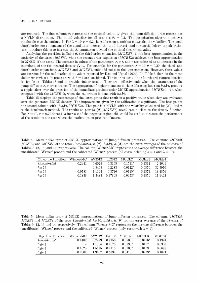
24 J. C. ARISMENDI
are reported. The first column σi represents the optimal volatility given the jump-diffusion price process hasa MVLN distribution. The initial volatility for all assets is σi = 0.2. The optimisation algorithm achievesresults close to the optimal σ. For λ = 10, ν = 0.2 the calibration algorithm outweighs the volatility. The smallfourth-order cross-moments of the simulation increase the total kurtosis and the methodology the algorithmuses to reduce this is to increase the σi parameters beyond the optimal theoretical value.
Analysing the precision in Table 9, the third-order expansion (MGEE3) is the best approximation in themajority of the cases (39.58%), while the second-order expansion (MGEE2) achieves the best approximationin 27.08% of the cases. The increase in values of the parameters λ, ν, t, and r are reflected as an increase in thecumulants of the risk-neutral density fX(t). For example, for the parameters λ = 10, ν = 0.20, the third- andfourth-order expansions, MGEE3 and MGEE4, only add noise to the approximation. However, these valuesare extreme for the real market data values reported by Das and Uppal (2004). In Table 5 there is the meandollar error when only processes with λ = 1 are considered. The improvement in the fourth-order approximationis significant. Tables 13 and 14 provide similar results. They are ineffective only when the parameters of thejump-diffusion λ, ν are extreme. The aggregation of higher moments in the calibrating function hi(σ), producea ripple effect over the precision of the immediate previous-order MGEE approximation MGEE(i − 1), whencompared with the MGEE(i), when the calibration is done with hi(σ).
Table 15 displays the percentage of simulated paths that result in a positive value when they are evaluatedover the generated MGEE density. The improvement given by the calibration is significant. The best pair isthe second column with (h2(σ),MGEE2). This pair is a MVLN with the volatility calculated by (20), and itis the benchmark method. The results on pair (h3(σ),MGEE3) reveal results close to the density function.For λ = 10, ν = 0.20 there is a increase of the negative region; this could be used to measure the performanceof the results in the case where the market option price is unknown.
Table 4: Mean dollar error of MGEE approximations of jump-diffusion processes. The columns MGEE2,MGEE3, and MGEE4 of the rows Uncalibrated, h2(σ), h3(σ), h4(σ) are the error-averages of the 48 cases ofTables 9, 12, 13, and 14, respectively. The column ‘Wiener-MC’ represents the average difference between theuncalibrated ‘Wiener’ process and the calibrated ‘Wiener’ process (all cases including λ = 1 and λ = 10).
Objective Function Wiener-MC AV2012 Li2012 MGEE2 MGEE3 MGEE4Uncalibrated 0.2441 0.6028 0.3105 0.1531∗ 0.3312 2.4641h2(σ) - 0.8468 0.2283 0.0122∗ 0.0870 32.5970h3(σ) 0.0783 1.1194 0.3736 0.0115∗ 0.1371 18.4856h4(σ) 0.1838 1.3484 0.47868 0.0353∗ 0.1856 11.1462
Table 5: Mean dollar error of MGEE approximations of jump-diffusion processes. The columns MGEE2,MGEE3 and MGEE4 of the rows Uncalibrated, h2(σ), h3(σ), h4(σ) are the error-averages of the 48 cases ofTables 9, 12, 13 and 14, respectively. The column ‘Wiener-MC’ represents the average difference between theuncalibrated ‘Wiener’ process and the calibrated ‘Wiener’ process (only cases with λ = 1).
Objective Function Wiener-MC AV2012 Li2012 MGEE2 MGEE3 MGEE4Uncalibrated 0.1402 0.7479 0.2156 0.0506 0.0426∗ 0.1374h2(σ) - 1.1364 0.2073 0.0133∗ 0.0157 0.0303h3(σ) 0.1028 1.5575 0.4113 0.0103∗ 0.0159 0.0699h4(σ) 0.2607 1.9107 0.5734 0.0418 0.0279∗ 0.1021
24
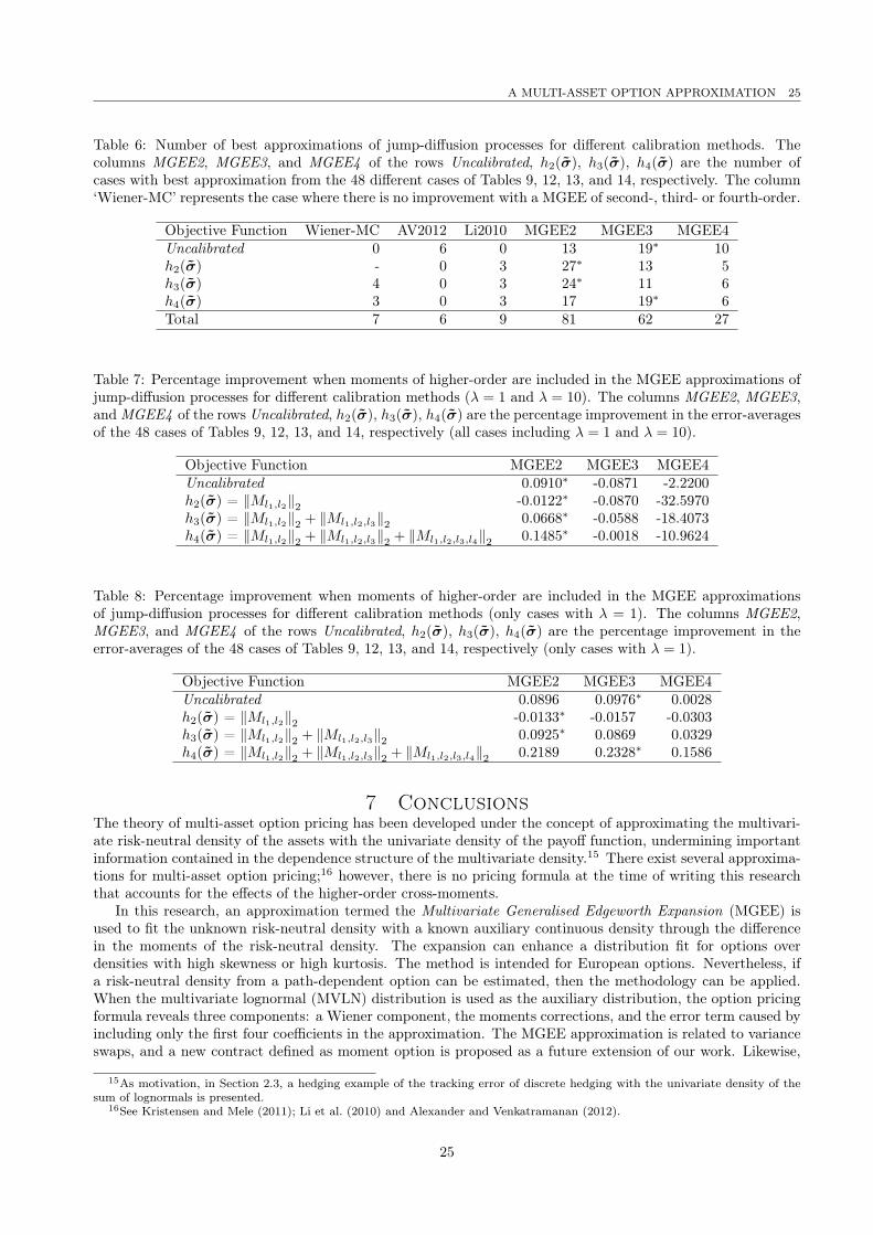
A MULTI-ASSET OPTION APPROXIMATION 25
Table 6: Number of best approximations of jump-diffusion processes for different calibration methods. Thecolumns MGEE2, MGEE3, and MGEE4 of the rows Uncalibrated, h2(σ), h3(σ), h4(σ) are the number ofcases with best approximation from the 48 different cases of Tables 9, 12, 13, and 14, respectively. The column‘Wiener-MC’ represents the case where there is no improvement with a MGEE of second-, third- or fourth-order.
Objective Function Wiener-MC AV2012 Li2010 MGEE2 MGEE3 MGEE4Uncalibrated 0 6 0 13 19∗ 10h2(σ) - 0 3 27∗ 13 5h3(σ) 4 0 3 24∗ 11 6h4(σ) 3 0 3 17 19∗ 6Total 7 6 9 81 62 27
Table 7: Percentage improvement when moments of higher-order are included in the MGEE approximations ofjump-diffusion processes for different calibration methods (λ = 1 and λ = 10). The columns MGEE2, MGEE3,and MGEE4 of the rows Uncalibrated, h2(σ), h3(σ), h4(σ) are the percentage improvement in the error-averagesof the 48 cases of Tables 9, 12, 13, and 14, respectively (all cases including λ = 1 and λ = 10).
Objective Function MGEE2 MGEE3 MGEE4Uncalibrated 0.0910∗ -0.0871 -2.2200h2(σ) = ∥Ml1,l2∥2 -0.0122∗ -0.0870 -32.5970h3(σ) = ∥Ml1,l2∥2 + ∥Ml1,l2,l3∥2 0.0668∗ -0.0588 -18.4073h4(σ) = ∥Ml1,l2∥2 + ∥Ml1,l2,l3∥2 + ∥Ml1,l2,l3,l4∥2 0.1485∗ -0.0018 -10.9624
Table 8: Percentage improvement when moments of higher-order are included in the MGEE approximationsof jump-diffusion processes for different calibration methods (only cases with λ = 1). The columns MGEE2,MGEE3, and MGEE4 of the rows Uncalibrated, h2(σ), h3(σ), h4(σ) are the percentage improvement in theerror-averages of the 48 cases of Tables 9, 12, 13, and 14, respectively (only cases with λ = 1).
Objective Function MGEE2 MGEE3 MGEE4Uncalibrated 0.0896 0.0976∗ 0.0028h2(σ) = ∥Ml1,l2∥2 -0.0133∗ -0.0157 -0.0303h3(σ) = ∥Ml1,l2∥2 + ∥Ml1,l2,l3∥2 0.0925∗ 0.0869 0.0329h4(σ) = ∥Ml1,l2∥2 + ∥Ml1,l2,l3∥2 + ∥Ml1,l2,l3,l4∥2 0.2189 0.2328∗ 0.1586
7 ConclusionsThe theory of multi-asset option pricing has been developed under the concept of approximating the multivari-ate risk-neutral density of the assets with the univariate density of the payoff function, undermining importantinformation contained in the dependence structure of the multivariate density.15 There exist several approxima-tions for multi-asset option pricing;16 however, there is no pricing formula at the time of writing this researchthat accounts for the effects of the higher-order cross-moments.
In this research, an approximation termed the Multivariate Generalised Edgeworth Expansion (MGEE) isused to fit the unknown risk-neutral density with a known auxiliary continuous density through the differencein the moments of the risk-neutral density. The expansion can enhance a distribution fit for options overdensities with high skewness or high kurtosis. The method is intended for European options. Nevertheless, ifa risk-neutral density from a path-dependent option can be estimated, then the methodology can be applied.When the multivariate lognormal (MVLN) distribution is used as the auxiliary distribution, the option pricingformula reveals three components: a Wiener component, the moments corrections, and the error term caused byincluding only the first four coefficients in the approximation. The MGEE approximation is related to varianceswaps, and a new contract defined as moment option is proposed as a future extension of our work. Likewise,
15As motivation, in Section 2.3, a hedging example of the tracking error of discrete hedging with the univariate density of thesum of lognormals is presented.
16See Kristensen and Mele (2011); Li et al. (2010) and Alexander and Venkatramanan (2012).
25
26 J. C. ARISMENDI
the partial derivatives of the expansion are sensitivities of the risk-neutral density against changes in its form,translation, dispersion, skewness, and heavy-tailedness, results that are important for future topics of research.
A multivariate Merton’s jump-diffusion process is used to test the MGEE option pricing approximation.There are two initial purposes for the approximation: the first is not obvious at first sight, and it is to findthe price premium that accounts for the difference in the moments. Risk managers could check whether thedifference in the price of two risk-neutral densities come from the second-order moments (greater volatility ofthe risk-neutral density), third-order moments (positive/negative bias, and bias of the density over an asset), orfourth-order moments (heavy-tailedness of the distribution). Several examples with dimension n = 2 and n = 5are presented in Sections 4.7 and 5.2, where the relationship between an increase in certain moments is relatedto the increase in price. The analytical multi-asset pricing methodologies of Li et al. (2010) and Alexanderand Venkatramanan (2012) were used for comparison purposes. The results show that when the informationprovided by the moments of the risk-neutral density is provided, the MGEE improves the results of a MonteCarlo methodology, and is superior to the Li et al. (2010) and Alexander and Venkatramanan (2012) analyticalapproximations.
The second purpose of the MGEE is the price approximation: a calibration over the MVLN auxiliarydensity parameters to reduce the moments’ differences with the risk-neutral density is proposed and developedin Section 6. The results of pricing the options over jump-diffusion processes show that the mean dollar errorfor the approximation could be of ∼ 1%−1.5% when only second-order moments are included in the expansion.These results include the extreme case17 of jump-diffusions with λ = 10. When the set examples are filtered tothe case of λ = 1, the mean dollar error when third- and fourth-order moments are included in the expansionimproves substantially. This is still a high parameter value for equity market returns. A major drawback of theMGEE expansion option pricing is the running performance of the algorithm, which is slow compared with theMonte Carlo algorithm (8 times slower when including the fourth-order moments in the expansion).
The results of this research are only the initial step to further investigations. Important extensions to ourwork include the development of a new theory for hedging the cross-moments of the risk-neutral density of multi-asset contract. The instruments to achieve this goal are defined as the moment options, and they require anextensive study and development. In a similar way, extensions to the theory of the sensitivity of the risk-neutraldistribution to changes in the moments is proposed as a considerable area of investigation.
Risk managers and hedgers will benefit from having an option formula that accounts for the moments of therisk-neutral distributions. Although the results are for general multi-assets contracts, the whole set of univariateoption contracts could enhance their performance if the theory of moments developed in this work were appliedto their pricing and hedging.
17Das and Uppal (2004) estimate a λ < 0.1 for emerging equity markets.
26

A MULTI-ASSET OPTION APPROXIMATION 27
ReferencesAlexander, C. and A. Venkatramanan (2011), ‘Closed form approximations for spread options’, Applied Math-
ematical Finance 18(5), 447–472.Alexander, C. and A. Venkatramanan (2012), ‘Analytic approximations for multi-asset option pricing’, Mathe-
matical Finance 22(4), 667–689.Arismendi, J.C. (2013), ‘Multivariate truncated moments’, Journal of Multivariate Analysis 117, 41–75.Aït-Sahalia, Y. and A. W. Lo (1998), ‘Nonparametric estimation of state-price densities implicit in financial
asset prices’, Journal of Finance 53(2), 499–547.Bates, D. S. (1991), ‘The crash of ’87: Was it expected? The evidence from options markets’, Journal of Finance
46(3), 1009–1044.Bhandari, R. and S. R. Das (2009), ‘Options on portfolios with higher-order moments’, Finance Research Letters
6, 122–129.Black, F. and M. Scholes (1973), ‘The pricing of options and corporate liabilities’, Journal of Political Economy
3(81), 637–654.Borovkova, S., F. J. Permana and H.V.D. Weide (2007), ‘A closed form approach to the valuation and hedging
of basket and spread option’, Journal of Derivatives 14(4), 8–24.Carmona, R. and V. Durrleman (2006), ‘Generalizing the Black–Scholes formula to multivariate contingent
claims’, Journal of Computational Finance 9(2), 627–685.Carr, P. (1988), ‘The valuation of sequential exchange opportunities’, Journal of Finance 43(5), 1235–1256.Corrado, C. J. and T. Su (1996), ‘S&P 500 index option tests of Jarrow and Rudd’s approximate option valuation
formula’, Journal of Futures Markets 16(6), 611–629.Das, S. R. and R. Uppal (2004), ‘Systemic risk and international portfolio choice’, Journal of Finance
59(6), 2809–2834.Del Brio, E. B., T.M. Ñíguez and J. Perote (2009), ‘Gram–Charlier densities: A multivariate approach’, Quan-
titative Finance 9(7), 855–868.Demeterfi, Kresimir, Emanuel Derman, Michael Kamal and Joseph Zou (1999), More than you ever wanted to
know about volatility swaps, Technical report, Goldman Sachs.Dufresne, D. (2004), ‘The log-normal approximation in financial and other computations’, Advances of Applied
Probability 36, 747–773.Filipović, D., E. Mayerhofer and P. Schneider (2013), ‘Density approximations for multivariate affine jump-
diffusion processes’, Journal of Econometrics 176(2), 93–111.Finney, D. J. (1963), ‘Some properties of a distribution specified by its cumulants’, Technometrics 5(1), 63–69.Flamouris, D. and D. Giamouridis (2002), ‘Estimating implied pdfs from American options on futures: A new
semiparametric approach’, Journal of Futures Markets 22(1), 1–30.Geske, R. (1979), ‘The valuation of compound options’, Journal of Financial Economics 7(1), 63 – 81.Harvey, C. R. and A. Siddique (2000), ‘Conditional skewness in asset pricing tests’, Journal of Finance
55(3), 1263–1295.Jarrow, R. and A. Rudd (1982), ‘Approximate option valuation for arbitrary stochastic processes’, Journal of
Financial Economics 10(3), 347–369.Ju, N. (2002), ‘Pricing Asian and basket options via Taylor expansion’, Journal of Computational Finance
5(3), 79–103.Kendall, M. G. (1947), The Advanced Theory of Statistics, Charles Griffin & Co.Kirk, E. (1996), ‘Correlation in energy markets’, in Managing Energy Price Risk pp. 71–78. Risk Publications.Knight, J. L. and S. Satchell (2001), ‘Pricing derivatives written on assets with arbitrary skewness and kurtosis’,
Return Distributions in Finance pp. 229–250. Butterworth and Heinemann.Kraus, A. and R. H Litzenberger (1976), ‘Skewness preference and the valuation of risk assets’, Journal of
Finance 31(4), 1085–1100.Kristensen, D. and A. Mele (2011), ‘Adding and subtracting Black-Scholes: A new approach to approximating
derivative prices in continuous-time models’, Journal of Financial Economics 102(2), 390–415.Li, M., S.J. Deng and J. Zhou (2008), ‘Closed-form approximations for spread option prices and Greeks’, Journal
of Derivatives 15(3), 58–80.Li, M., S.J. Deng and J. Zhou (2010), ‘Multi-asset spread option pricing and hedging’, Quantitative Finance
10(3), 305–324.Lim, G. C., G. M. Martin and V. L. Martin (2005), ‘Parametric pricing of higher order moments in S&P500
options’, Journal of Applied Econometrics 20(3), 377–404.
27
28 J. C. ARISMENDI
Limpert, E., W. A. Stahel and M. Abbt (2001), ‘Log-normal distributions across the sciences: Keys and clues’,Bioscience 51(5), 341–352.
Margrabe, W. (1978), ‘The value of an option to exchange one asset for another’, Journal of Finance 33(1), 177–186.
McCullagh, P. (1987), Tensor Methods in Statistics, Chapman & Hall.Merton, R. C. (1976), ‘Option pricing when underlying stock returns are discontinuous’, Journal of Financial
Economics 3(1-2), 125–144.Neuberger, A. (1994), ‘The log contract’, Journal of Portfolio Management 20(2), 74–80.Níguezy, T.-M. and J. Perote (2008), The general moments expansion: an application for financial risk. Plenary
Talk, ERCIM’ 08.Perote, J. (2004), ‘The multivariate Edgeworth–Sargan density’, Spanish Economic Review 6(1), 77–96.Rosenbaum, S. (1961), ‘Moments of a truncated bivariate normal distribution’, Journal of the Royal Statistical
Society. Series B (Methodological) 23(2), 405–408.Rubinstein, M. (1998), ‘Edgeworth binomial trees’, Journal of Derivatives 5(3), 20–27.Schleher, D.C. (1977), ‘Generalized gram-charlier series with application to the sum of log-normal variates’,
IEEE Transactions on Information Theory 1, 275–280.Schlögl, E. (2013), ‘Option pricing where the underlying assets follow a gram/charlier density of arbitrary order’,
Journal of Economic Dynamics & Control 37, 611–632.Schoutens, W. (2005), ‘Moment swaps’, Quantitative Finance 5(6), 525–530.Skovgaard, I.M. (1986), ‘On multivariate edgeworth expansions’, International Statistical Review 54(2), 169–
186.Tallis, G. M. (1961), ‘The moment generating function of the truncated multi-normal distribution’, Journal of
the Royal Statistical Society. Series B (Methodological) 23(1), 223–229.Zhao, H., J. E. Zhang and E.C. Chang (2013), ‘The relation between physical and risk-neutral cumulants’,
International Review of Finance 13(3), 345–381.
28

A MULTI-ASSET OPTION APPROXIMATION 29
Appendix A Analytical Proofs
A.1 Proof of Proposition 3.1Proof. Let fX be the continuous-time function density of X and ξ ∈ RN . The characteristic function (CF) ofX is defined as:
ψ(x, ξ) = E[exp
(ξ[l1]X[l1]i
)].
Denote ml1,...,lp(x) the p-moment of X. This function can be expanded into the infinite series:
ψ(x, ξ) = 1 + ξ[l1]m[l1](x)i+ ξ[l1]ξ[l2]m[l1,l2](x)i2/2! + ξ[l1]ξ[l2]ξ[l3]m[l1,l2,l3](x)i
3/3! + . . . , (21)
=
n−1∑j=1
ξ[l1] . . . ξ[lj ]m[l1,...,l2](x)ij/j! + o(∥ξ∥n),
which is convergent for small ξ. We calculate the log function:
logψ(x, ξ) =
n−1∑j=1
ξ[l1] . . . ξ[lj ]k[l1,[...,[lj ]... ](x)ij/j! + o(∥ξ∥n),
where kl1,...,lp(x) are the cumulants of order p of X. Now suppose that we have another continuous densityfunction gS of a stochastic process s. Then we can write:
logψ(x, ξ) =n−1∑j=1
ξ[l1] . . . ξ[lj ](k[l1,[...,[lj ]... ](x)− k[l1,[...,[lj ]... ](s))ij/j! +
n−1∑j=1
ξ[l1] . . . ξ[lj ]k[l1,[...,[lj ]... ](s)ij/j! + o(∥ξ∥n),
=n−1∑j=1
ξ[l1] . . . ξ[lj ](k[l1,[...,[lj ]... ](x)− k[l1,[...,[lj ]... ](s))ij/j! + logψ(s, ξ) + o(∥ξ∥n),
where kl1,...,lp(s) are the cumulants of order p of s. Applying the exponential function on both sides:
ψ(x, ξ) = exp
n−1∑j=1
ξ[l1] . . . ξ[lj ](k[l1,[...,[lj ]... ](x)− k[l1,[...,[lj ]... ](s))ij/j!
ψ(s, ξ) exp (o(∥ξ∥n)) .
It could be demonstrated that: exp(o(∥ξ∥n)) = 1 + o(∥ξ∥n). But the exponential function can be expanded asin (21). Then,
ψ(x, ξ) =
n−1∑j=0
ξ[l1] . . . ξ[lj ]M[l1,[...,[lj ]... ]ij/j!
ψ(s, ξ) + o(∥ξ∥n), (22)
where Ml1,...,lj are the difference of the moments of distributions fX, gS.The Fourier transforms of fX and gS are, respectively:
fX =1
2π
(n)∫ ∞
−∞exp(−iξ′x)ψ(x, ξ)dξ, (23)
gS =1
2π
(n)∫ ∞
−∞exp(−iξ′s)ψ(s, ξ)dξ, (24)
and the j-partial derivative of (24) is:
(−1)j∂j
∂sl1 . . . ∂sljgS =
1
2π
(n)∫ ∞
−∞exp(−iξ′s)ijξ[l1] . . . ξ[ij ]ψ(s, ξ)dξ. (25)
29
30 J. C. ARISMENDI
Applying the inverse Fourier transform to (22), we have that,
1
2π
(n)∫ ∞
−∞exp(−iξ′x)ψ(x, ξ)dξ =
1
2π
(n)∫ ∞
−∞exp(−iξ′s)
n−1∑j=0
ξ[l1] . . . ξ[lj ]M[l1,[...,[lj ]... ]ij/j!
ψ(s, ξ) + o(∥ξ∥n)
dξ.
Using (23), (24), and (25), it finally yields,
fX = gS +n−1∑j=1
M[l1,[...,[lj ]... ](−1)j
j!
∂j
∂sl1 . . . ∂sljgS + ε(s, n),
where
ε(s, n) =1
2π
(n)∫ ∞
−∞exp(iξ′s)o(∥ξ∥n)dξ.
A.2 First four partial derivatives of a MVLN distributionDenote Σ−1
s the inverse matrix of Σs as in (19) and define Λ = −12 (log(S)− µs)
′Σ−1
s (log(S)− µs). The firstfour terms of ∂j
∂Sl1...∂Slj
gS(t) are:The first-order partial derivative is,
∂
∂Sl1
gS = gS
(− 1
Sl1
+∂Λ
∂Sl1
), (26)
where,∂Λ
∂Sl1
= − 1
Sl1
Σ−1s,(l1,:)
(log (S)− µs)
and Σ−1s,(l1,:)
is the l1-th row of Σ−1s . The second-order partial derivatives of gS are,
∂2
∂S2l1
gS = gS
(2
S2l1
− 2
Sl1
∂Λ
∂Sl1
+
(∂Λ
∂Sl1
)2
+∂2Λ
∂S2l1
),
∂2
∂Sl1∂Sl2
gS = gS
(1
Sl1Sl2
− 1
Sl1
∂Λ
∂Sl2
− 1
Sl2
∂Λ
∂Sl1
+∂Λ
∂Sl1
∂Λ
∂Sl2
+∂2Λ
∂Sl1∂Sl2
), (27)
where,
∂2Λ
∂S2l1
=1
S2l1
(Σ−1
s,(l1,:)(log (S)− µs)− ςl1,l1
),
∂2Λ
∂Sl1∂Sl2
= − 1
Sl1Sl2
ςl1,l2 ,
The third-order partial derivatives of gS are,
∂3
∂S3l1
gS = gS
(− 6
S3l1
+6
S2l1
∂Λ
∂Sl1
− 3
Sl1
(∂Λ
∂Sl1
)2
− 3
Sl1
∂2Λ
∂S2l1
+ 3∂Λ
∂Sl1
∂2Λ
∂S2l1
+
(∂Λ
∂Sl1
)3
+∂3Λ
∂S3l1
),
∂3
∂S2l1∂Sl2
gS =
((− 1
Sl2
+∂Λ
∂Sl2
)∂2
∂S2l1
gS − gS
(2
Sl1
∂2Λ
∂Sl1∂Sl2
+ 2∂Λ
∂Sl1
∂2Λ
∂Sl1∂Sl2
+∂3Λ
∂S2l1∂Sl2
)),
∂3
∂Sl1∂Sl2∂Sl3
gS =
((− 1
Sl3
+∂Λ
∂Sl3
)∂2
∂Sl1∂Sl2
gS +
gS
(− 1
Sl1
∂2Λ
∂Sl2∂Sl3
− 1
Sl2
∂2Λ
∂Sl1∂Sl3
+∂2Λ
∂Sl2∂Sl3
∂Λ
∂Sl1
+∂Λ
∂Sl2
∂2Λ
∂Sl1∂Sl3
)), (28)
30
A MULTI-ASSET OPTION APPROXIMATION 31
where,
∂3Λ
∂S3l1
=1
S3l1
(−2Σ−1
s,(l1,:)(log (S)− µs) + 3ςl1,l1
),
∂3Λ
∂S2l1∂Sl2
=1
S2l1Sl2
ςl1,l2 .
The term ∂3Λ∂Sl1
∂Sl2∂Sl3
is equal to zero.And the fourth-order partial derivatives of gS are,
∂4
∂S4l1
gS = gS
(24
S4l1
− 24
S3l1
∂Λ
∂Sl1
+12
S2l1
(∂2Λ
∂S2l1
)+
12
S2l1
(∂Λ
∂Sl1
)2
− 12
Sl1
∂Λ
∂Sl1
∂2Λ
∂S2l1
− 4
Sl1
∂3Λ
∂S3l1
+
3
(∂2Λ
∂S2l1
)2
+ 4∂Λ
∂Sl1
∂3Λ
∂S3l1
+ 6
(∂Λ
∂Sl1
)2∂2Λ
∂S2l1
− 4
Sl1
(∂Λ
∂Sl1
)3
+
(∂Λ
∂Sl1
)4
+∂4Λ
∂S4l1
),
∂4
∂S3l1∂Sl2
gS =
((− 1
Sl2
+∂Λ
∂Sl2
)∂3
∂S3l1
gS + gS
(6
S2l1
∂2Λ
∂Sl1∂Sl2
− 6
Sl1
∂Λ
∂Sl1
∂2Λ
∂Sl1∂Sl2
− 3
Sl1
∂3Λ
∂S2l1∂Sl2
+
3∂2Λ
∂Sl1∂Sl2
∂2Λ
∂S2l1
+ 3∂Λ
∂Sl1
∂3Λ
∂S2l1∂Sl2
+ 3
(∂Λ
∂Sl1
)2∂2Λ
∂Sl1∂Sl2
+∂4Λ
∂S3l1∂Sl2
)),
∂4
∂S2l1∂S2
l2
gS =
((− 1
Sl2
+∂Λ
∂Sl2
)∂3
∂S2l1∂Sl2
gS + gS
(2
S2l1S2l2
− 2
Sl1S2l2
∂Λ
∂Sl1
+2
Sl1Sl2
∂2Λ
∂Sl1∂Sl2
+
1
S2l2
(∂Λ
∂Sl1
)2
− 2
Sl2
∂Λ
∂Sl1
∂2Λ
∂Sl1∂Sl2
+1
S2l2
∂2Λ
∂S2l1
− 1
Sl2
∂3Λ
∂S2l1∂Sl2
+2
S2l1
∂2Λ
∂S2l2
−
2
Sl1
∂2Λ
∂Sl1∂Sl2
∂Λ
∂Sl2
− 2
Sl1
∂Λ
∂Sl1
∂2Λ
∂S2l2
+ 2∂Λ
∂Sl1
∂2Λ
∂Sl1∂Sl2
∂Λ
∂Sl2
+
(∂Λ
∂Sl1
)2∂2Λ
∂S2l2
+
∂3Λ
∂S2l1∂Sl2
∂Λ
∂Sl2
+∂2Λ
∂S2l1
∂2Λ
∂S2l2
− 2
Sl1
∂3Λ
∂Sl1∂S2l2
+ 2∂Λ
∂Sl1
∂3Λ
∂Sl1∂S2l2
+∂4Λ
∂S2l1∂S2
l2
)),
∂4
∂S2l1∂Sl2∂Sl3
gS =
((− 1
Sl3
+∂Λ
∂Sl3
)∂3
∂S2l1∂Sl2
gS + gS
(2
Sl1Sl2
∂2Λ
∂Sl1∂Sl3
− 2
Sl2
∂Λ
∂Sl1
∂2Λ
∂Sl1∂Sl3
− 1
Sl2
∂3Λ
∂S2l1∂Sl3
+
2
S2l1
∂2Λ
∂Sl2∂Sl3
− 2
Sl1
∂Λ
∂Sl2
∂2Λ
∂Sl1∂Sl3
− 2
Sl1
∂Λ
∂Sl1
∂2Λ
∂Sl2∂Sl3
+ 2∂Λ
∂Sl1
∂2Λ
∂Sl1∂Sl3
∂Λ
∂Sl2
+(∂Λ
∂Sl1
)2∂2Λ
∂Sl2∂Sl3
+∂3Λ
∂S2l1∂Sl3
∂Λ
∂Sl2
+∂2Λ
∂S2l1
∂2Λ
∂Sl2∂Sl3
+∂2Λ
∂Sl1∂Sl3
∂2Λ
∂Sl1∂Sl2
)),
∂4
∂Sl1∂Sl2∂Sl3∂Sl4
gS =
((− 1
Sl4
+∂Λ
∂Sl4
)∂3
∂Sl1∂Sl2∂Sl3
gS + gS
(1
Sl1Sl3
∂2Λ
∂Sl2∂Sl4
+1
Sl2Sl3
∂2Λ
∂Sl1∂Sl4
+
1
Sl1Sl2
∂2Λ
∂Sl3∂Sl4
− 1
Sl3
∂2Λ
∂Sl2∂Sl4
∂Λ
∂Sl1
− 1
Sl3
∂Λ
∂Sl2
∂2Λ
∂Sl1∂Sl4
− 1
Sl1
∂2Λ
∂Sl2∂Sl4
∂Λ
∂Sl3
−
1
Sl1
∂2Λ
∂Sl3∂Sl4
∂Λ
∂Sl2
− 1
Sl2
∂2Λ
∂Sl1∂Sl4
∂Λ
∂Sl3
− 1
Sl2
∂2Λ
∂Sl3∂Sl4
∂Λ
∂Sl1
+∂2Λ
∂Sl1∂Sl4
∂Λ
∂Sl2
∂Λ
∂Sl3
+
∂2Λ
∂Sl2∂Sl4
∂Λ
∂Sl1
∂Λ
∂Sl3
+∂2Λ
∂Sl3∂Sl4
∂Λ
∂Sl1
∂Λ
∂Sl2
+∂2Λ
∂Sl3∂Sl4
∂2Λ
∂Sl1∂Sl2
+
∂2Λ
∂Sl3∂Sl2
∂2Λ
∂Sl1∂Sl4
+∂2Λ
∂Sl2∂Sl4
∂2Λ
∂Sl1∂Sl3
)), (29)
31
32 J. C. ARISMENDI
where,
∂4Λ
∂S4l1
=1
S4l1
(6Σ−1
s,(l1,:)(log (S)− µs)− 11ςl1,l1
),
∂4Λ
∂S3l1∂Sl2
= − 2
S3l1Sl2
ςl1,l2 ,
∂4Λ
∂S2l1∂S2
l2
= − 1
S2l1S2l2
ςl1,l2 .
The terms ∂4Λ∂S2
l1∂Sl2
∂Sl3
and ∂4Λ∂Sl1
∂Sl2∂Sl3
∂Sl4are equal to zero.
A.3 Analysis of the correction term C0,W,[l1,...,lj ] (Π(x(t)))The first-order partial derivative of gS is,
∂
∂Sl1
gS = gS
(− 1
Sl1
+∂Λ
∂Sl1
)= gS
(− 1
Sl1
)(1 + Σ−1
s,(l1,:)log (s)− Σ−1
s,(l1,:)µs
), (30)
where Σ−1s,(l1,:)
is the l1-th row of Σ−1s .
Disentangling the partial derivative we get:1a. The terms gS
(− 1
Sl1
)and gS
(− 1
Sl1
)Σ−1
s,(l1,:)µs could be re-expressed as MVLN densities:
Proposition A.1. Let S(t) = (S1(t), . . . , Sn(t)) be a multivariate GBM process defined as in (1), with MVLNdistribution and parameters µs,Σs, the conditional expected value:
EQ0
[log(S1(t))
α1 . . . log(Sn(t))αnS1(t)
β1 . . . Sn(t)βn |Sj(t) ≥ K
],
with j ∈ 1, . . . , n, αi, βi ∈ I, is equal to the lower truncated moment of a MVN process Y(t) = (Y1(t), . . . , Yn(t))times a constant A:
A ·EQ0 [Y1(t)
α1 . . . Yn(t)αn |Yj(t) ≥ log(K)] ,
where Y(t) ∼ N (µs +Σsβ,Σs).Proof. Applying the definition of the MVLN, and after the change of variable Si = exp(Yi), we have the
resulting moment over the MVN distribution:
EQ0
[log(S1(t))
α1 . . . log(Sn(t))αnS1(t)
β1 . . . Sn(t)βn |Sj(t) ≥ K
]=
= L−11
((n−1)∫ ∞
0
∫ ∞
K
(2π)−n/2|Σs|−1/2
(n∏
i=1
log(si)αi
)(n∏
i=1
sβi−1i
)exp
(−1
2(log(s)− µs)
′Σ−1
s (log(s)− µs)
)ds
)
= L−11
((n−1)∫ ∞
−∞
∫ ∞
log(K)
(2π)−n/2|Σs|−1/2
(n∏
i=1
yαii
)exp (y′β) exp
(−1
2(y − µs)
′Σ−1
s (y − µs)
)dy
),
where L1 = PQ (Sj(t) ≥ K). The time parameter of the process Y(t) is omitted to simplify the notation. Thelast expression can be transformed as:
= L−11
((n−1)∫ ∞
−∞
∫ ∞
log(K)
(2π)−n/2|Σs|−1/2
(n∏
i=1
yαii
)exp
(1
2β′Σsβ + β′µs −
1
2(y − ζ)
′Σs
−1 (y − ζ)
)dy
),
with ζ = µs +Σsβ. Define L2 = PQ (Yj(t) ≥ log(K)), then the last expression becomes:
= exp
(1
2β′Σsβ + β′µs
)(L2
L1
)E
Q0 [Y1(t)
α1 . . . Yn(t)αn |Yj(t) ≥ log(K)] .
32

A MULTI-ASSET OPTION APPROXIMATION 33
Then the variable Y(t) is distributed N (µs +Σsβ,Σs), the constant A = exp(12β
′Σsβ + β′µs
) (L2
L1
)and the
result follows.
Corollary A.2. Let gS have the multivariate density as in (17). Denote α = (α1, . . . , αn) a vector of integers.The function:
gS = Sα11 . . . Sαn
n gS,
is a MVLN density function and can be re-written as:
gS = exp(µ′sα)gS,
Proof. With some algebraic calculations it follows from Proposition (A.1).
Then, the terms gS(− 1
Sl1
)and gS
(− 1
Sl1
)Σ−1
s,(l1,:)µs are MLVN densities, setting αl1 = −1, αi = 0, i ∈
1, . . . , n, i = l1 in Corollary (A.2), and we have the resulting density:
gS = −gS(
1
Sl1
)= exp(−µ1)gS,
The term Σ−1s,(l1,:)
µs is an scalar value, it is the dot product of two vectors.
1b. The term gS
(− 1
Sl1
)Σ−1
s,(l1,:)log (s) is a sum of MVLN densities times a log-contract.
The first-order moment correction of (18) becomes:
exp(−rt)n∑
l1=1
Ml1(−1)(n)∫ ∞
0
Π(s(t))∂
∂Sl1
gS =
exp(−rt)
(n∑
l1=1
Ml1(−1)(Σ−1s,(l1,:)
µs − 1) exp(−µl1)(n)∫ ∞
0
Π(s(t))gS +
n∑l1=1
Ml1(−1) exp(−µl1)n∑
j=1
ςl1,j
(n)∫ ∞
0
log(Sj)Π(s(t))gS
).
The second-order partial derivative of gS against the same variable is:
∂2
∂S2l1
gS = gS
(2
S2l1
− 2
Sl1
∂Λ
∂Sl1
+
(∂Λ
∂Sl1
)2
+∂2Λ
∂S2l1
)
= gS
(1
S2l1
)(2 + 2
(Σ−1
s,(l1,:)log (s)− Σ−1
s,(l1,:)µs
)+(Σ−1
s,(l1,:)log (s)− Σ−1
s,(l1,:)µs
)2+
(Σ−1
s,(l1,:)log (s)− Σ−1
s,(l1,:)µs − ςl1,l1
)),
= gS
(1
S2l1
)((2− 3Σ−1
s,(l1,:)µs +
(Σ−1
s,(l1,:)µs
)2− ςl1,l1
)+Σ−1
s,(l1,:)log (s)
(3− 2Σ−1
s,(l1,:)µs
)+
(Σ−1
s,(l1,:)log (s)
)2). (31)
Unfolding we get three terms:
2a. The term gS
(1
S2l1
)(2− 3Σ−1
s,(l1,:)µs +
(Σ−1
s,(l1,:)µs
)2− ςl1,l1
)could be re-written as a MVLN density:
In this case, set αl1 = −2, αi = 0, i ∈ 1, . . . , n, i = l1 in the Corollary (A.2), and the resulting density
33

34 J. C. ARISMENDI
yields:
gS = gS
(1
S2l1
)(2− 3Σ−1
s,(l1,:)µs +
(Σ−1
s,(l1,:)µs
)2− ςl1,l1
)= exp(−2µl1)
(2− 3Σ−1
s,(l1,:)µs +
(Σ−1
s,(l1,:)µs
)2− ςl1,l1
)gS.
2b. The term gS
(1
S2l1
)Σ−1
s,(l1,:)log (s)
(3− 2Σ−1
s,(l1,:)µs
)is a sum of MVLN densities times a log-contract.
2c. The term gS
(1
S2l1
)(Σ−1
s,(l1,:)log (s)
)2is a sum of MVLN densities times quadratic functions of log-
contracts.
Resuming we have the second-order moment correction of (18) with the same index l1 is:
exp(−rt)n∑
l1=1
Ml1,l1
1
2
(n)∫ ∞
0
Π(s(t))∂2
∂S2l1
gS =
exp(−rt)
(n∑
l1=1
Ml1,l1
1
2exp(−2µl1)
(2− 3Σ−1
s,(l1,:)µs +
(Σ−1
s,(l1,:)µs
)2− ςl1,l1
) (n)∫ ∞
0
Π(s(t))gS +
n∑l1=1
Ml1,l1
1
2exp(−2µl1)
(3− 2Σ−1
s,(l1,:)µs
) n∑j=1
(ςl1,j)(n)∫ ∞
0
Π(s(t)) log(Sj)gS +
n∑l1=1
Ml1,l1
1
2exp(−2µl1)
n∑j1=1
(ςl1,j1)2(n)∫ ∞
0
Π(s(t)) log(Sj1)2gS
).
The second-order mixed partial derivative of gS is:
∂2
∂Sl1∂Sl2
gS = gS
(1
Sl1Sl2
− 1
Sl1
∂Λ
∂Sl2
− 1
Sl2
∂Λ
∂Sl1
+∂Λ
∂Sl1
∂Λ
∂Sl2
+∂2Λ
∂Sl1∂Sl2
)= gS
(1
Sl1Sl2
)(1 +
(Σ−1
s,(l1,:)log (s)− Σ−1
s,(l1,:)µs
)+(Σ−1
s,(l2,:)log (s)− Σ−1
s,(l2,:)µs
)+
(Σ−1
s,(l1,:)log (s)− Σ−1
s,(l1,:)µs
)(Σ−1
s,(l2,:)log (s)− Σ−1
s,(l2,:)µs
)− ςl1,l2
)
= gS
(1
Sl1Sl2
)((1− Σ−1
s,(l1,:)µs − Σ−1
s,(l2,:)µs +Σ−1
s,(l1,:)µsΣ
−1s,(l2,:)
µs − ςl1,l2
)+
log (s)′(Σ−1
s,(l1,:)
(1− Σ−1
s,(l2,:)µs
)+Σ−1
s,(l2,:)
(1− Σ−1
s,(l1,:)µs
))+(Σ−1
s,(l1,:)log (s)Σ−1
s,(l2,:)log (s)
)). (32)
Re-arranging we get:2a. The term gS
(1
Sl1Sl2
)(1− Σ−1
s,(l1,:)µs − Σ−1
s,(l2,:)µs +Σ−1
s,(l1,:)µsΣ
−1s,(l2,:)
µs − ςl1,l2
)setting αl1 = −1, αl2 =
−1, αi = 0, i ∈ 1, . . . , n, i = l1 = l2 and applying the Corollary (A.2), could be transformed as MVLNdensities:
gS = gS
(1
Sl1Sl2
)(1− Σ−1
s,(l1,:)µs − Σ−1
s,(l2,:)µs +Σ−1
s,(l1,:)µsΣ
−1s,(l2,:)
µs − ςl1,l2
)= exp(−µl1 − µl2)
(1− Σ−1
s,(l1,:)µs − Σ−1
s,(l2,:)µs +Σ−1
s,(l1,:)µsΣ
−1s,(l2,:)
µs − ςl1,l2
)gS.
2b. Log-contracts times MVLN densities,
gS
(1
Sl1Sl2
)log (s)
′(Σ−1
s,(l1,:)
(1− Σ−1
s,(l2,:)µs
)+Σ−1
s,(l2,:)
(1− Σ−1
s,(l1,:)µs
)).
34

A MULTI-ASSET OPTION APPROXIMATION 35
2c. Cross log-contracts of second-order, that will appear when calculating cross-sensitivities of the MVLNdensity:
gS
(1
Sl1Sl2
)(Σ−1
s,(l1,:)log (s)Σ−1
s,(l2,:)log (s)
).
Finally, the second-order mixed moment correction is:
exp(−rt)n∑
l1=1
n∑l1=2
Ml1,l2
1
2
(n)∫ ∞
0
Π(s(t))∂2
∂S2l1
gS = exp(−rt)(n∑
l1=1
n∑l2=1
Ml1,l2
1
2exp(−µl1 − µl2)
(1− Σ−1
s,(l1,:)µs − Σ−1
s,(l2,:)µs +Σ−1
s,(l1,:)µsΣ
−1s,(l2,:)
µs − ςl1,l2
) (n)∫ ∞
0
Π(s(t))gS +
n∑l1=1
n∑l2=1
Ml1,l2
1
2exp(−µl1 − µl2)
n∑j=1
(ςj,l1
(1− Σ−1
s,(l2,:)µs
)+ ςl2,j
(1− Σ−1
s,(l1,:)µs
)) (n)∫ ∞
0
Π(s(t)) log(Sj)gS +
n∑l1=1
n∑l2=1
Ml1,l2
1
2exp(−µl1 − µl2)
n∑j1=1
n∑j2=1
(ςl1,j1ςl2,j2)(n)∫ ∞
0
Π(s(t)) log(Sj1) log(Sj2)gS
).
35

36 J. C. ARISMENDI
Appendix B Tables
Table 9: Option prices with a MGEE of jump-diffusion processes. The risk-neutral density fX(t) is gener-ated by a 5-dimensional jump-diffusion process with parameters λ = 10, δi = 0, νi = 0.05, r = 0.10, t =0.25, σi = 0.2, (S1(0), . . . , S5(0)) = (35, 25, 20, 15, 5), i ∈ 1, . . . , 5. The payoff of the basket option is
Π(S(t)) =(∑5
i=1 Si(t)−K)+
with K ∈ 90, 100, 110. The mean parameters of the auxiliary MVLN densitygS(t) are set by the arbitrage-free constraints, and the volatility parameters are set equal to the jump-diffusionprocess. The best approximation is highlighted.
λ ν t K r J-D Wiener AV2012 Li2010 MGEE2 MGEE3 MGEE4
90 0.05 11.256 11.133 11.464 11.124 11.209∗ 11.092 11.4260.10 12.315 12.229 12.457 12.224 12.282∗ 12.209 12.458
0.25 100 0.05 3.384 2.667 2.779 2.463 3.752 3.655∗ 2.7220.10 4.105 3.446 3.550 3.265 4.470 4.247∗ 3.259
110 0.05 0.540 0.110 1.178 0.058 0.356 0.565∗ 0.9310.20 0.10 0.699 0.192 1.474 0.115 0.562 0.825∗ 1.247
90 0.05 15.273 14.629 15.023 14.527 15.542 14.682 15.330∗
0.10 18.967 18.628 18.839 18.595 19.039∗ 18.493 19.7161.00 100 0.05 8.293 6.818 7.018 6.448 9.089 8.631∗ 6.731
0.10 11.395 10.308 10.488 10.079 12.103 11.140∗ 10.519110 0.05 3.865 2.206 3.509 1.790 4.194 4.867 4.098∗
1 0.10 5.920 4.241 5.577∗ 3.798 6.750 6.932 4.90490 0.05 11.134 11.131 11.464 11.124 11.136 11.135∗ 11.156
0.10 12.230 12.229 12.457 12.224 12.231 12.230∗ 12.2130.25 100 0.05 2.724 2.667 2.779 2.463 2.730 2.728∗ 2.755
0.10 3.498 3.446 3.550 3.265 3.506 3.502 3.494∗
110 0.05 0.128 0.109 1.178 0.058 0.124∗ 0.119 0.2070.05 0.10 0.218 0.192 1.474 0.115 0.213 0.222∗ 0.191
90 0.05 14.665 14.630 15.023 14.527 14.683 14.653∗ 14.6360.10 18.644 18.625 18.839 18.595 18.649∗ 18.626 18.572
1.00 100 0.05 6.926 6.817 7.018 6.448 6.949 6.932∗ 6.9870.10 10.382 10.307 10.488 10.079 10.409 10.370∗ 10.408
110 0.05 2.327 2.207 3.509 1.790 2.322∗ 2.344 2.3600.10 4.367 4.240 5.577 3.798 4.385∗ 4.392 4.493
90 0.05 13.288 11.130 11.464 11.124 12.017∗ 9.661 33.8890.10 14.106 12.229 12.457 12.224 12.660∗ 11.033 32.494
0.25 100 0.05 7.313 2.666 2.779 2.463 14.064 11.768∗ -55.1310.10 7.918 3.444 3.550 3.265 14.140 8.409∗ -47.872
110 0.05 3.691 0.110 1.178 0.058 2.692∗ 7.666 33.7440.20 0.10 4.068 0.192 1.474 0.115 4.096∗ 10.746 35.706
90 0.05 21.339 14.628 15.023 14.527 25.961∗ -23.295 192.0380.10 23.930 18.627 18.839 18.595 23.455∗ -5.724 289.794
1.00 100 0.05 16.296 6.815 7.018 6.448 34.696 7.941∗ -510.0660.10 18.613 10.309 10.488∗ 10.079 32.198 -22.548 -205.431
110 0.05 12.351 2.206 3.509∗ 1.790 26.454 65.142 -166.41610 0.10 14.345 4.238 5.577∗ 3.798 78.379 84.349 -512.313
90 0.05 11.196 11.132 11.464 11.124 11.176 11.157 11.196∗
0.10 12.267 12.230 12.457 12.224 12.255 12.245 12.272∗
0.25 100 0.05 3.196 2.666 2.779 2.463 3.299 3.277 3.259∗
0.10 3.934 3.445 3.550 3.265 4.041 3.995 3.935∗
110 0.05 0.318 0.110 1.178 0.058 0.254 0.295 0.331∗
0.05 0.10 0.465 0.192 1.474 0.115 0.408 0.462∗ 0.48790 0.05 15.033 14.625 15.023∗ 14.527 15.161 14.899 15.110
0.10 18.829 18.629 18.839∗ 18.595 18.865 18.691 19.1391.00 100 0.05 7.806 6.814 7.018 6.448 8.142 8.008∗ 7.449
0.10 11.029 10.306 10.488 10.079 11.341 11.051∗ 10.881110 0.05 3.273 2.206 3.509 1.790 3.361 3.563 3.347∗
0.10 5.358 4.242 5.577 3.798 5.705 5.753 5.216∗
36

A MULTI-ASSET OPTION APPROXIMATION 37
Table 10: Volatility values obtained from the minimisation of h3(σ) following the calibration algorithm describedin Section 6.1. The volatilities σi are components of the volatility vector that correspond to each case of Table13. As the strike price K does not affect the minimisation algorithm, there are only 16 vectors corresponding tothe 48 cases. The column σi represents the optimal volatility vector for the auxiliary MVLN distribution whenthe constraint of equal components is imposed.
λ ν t r σi σ1 σ2 σ3 σ4 σ5
0.25 0.05 0.2828 0.3608 0.3619 0.3621 0.3664 0.34850.20 0.10 0.2828 0.3611 0.3612 0.3642 0.3665 0.3566
1.00 0.05 0.2828 0.3128 0.3119 0.3134 0.3142 0.31751 0.10 0.2828 0.3136 0.3130 0.3130 0.3132 0.3225
0.25 0.05 0.2062 0.2077 0.2064 0.2107 0.2142 0.23090.05 0.10 0.2062 0.2055 0.2044 0.2035 0.2013 0.1654
1.00 0.05 0.2062 0.2068 0.2073 0.2085 0.2084 0.21440.10 0.2062 0.2067 0.2064 0.2082 0.2080 0.2204
0.25 0.05 0.6633 0.7572 0.7582 0.7579 0.7592 0.77480.20 0.10 0.6633 0.7575 0.7579 0.7585 0.7575 0.7618
1.00 0.05 0.6633 0.7181 0.7140 0.7093 0.7141 0.714210 0.10 0.6633 0.7173 0.7139 0.7093 0.7147 0.7062
0.25 0.05 0.2550 0.2603 0.2610 0.2603 0.2573 0.30160.05 0.10 0.2550 0.2602 0.2603 0.2624 0.2587 0.2193
1.00 0.05 0.2550 0.2566 0.2551 0.2545 0.2577 0.25700.10 0.2550 0.2566 0.2553 0.2547 0.2559 0.2442
Table 11: Volatility values obtained from the minimisation of h4(σ) following the calibration algorithm describedin Section 6.1. The volatilities σi are components of the volatility vector that correspond to each case of Table14. As the strike price K does not affect the minimisation algorithm, there are only 16 vectors corresponding tothe 48 cases. The column σi represents the optimal volatility vector for the auxiliary MVLN distribution whenthe constraint of equal components is imposed.
λ ν t r σi σ1 σ2 σ3 σ4 σ5
0.25 0.05 0.2828 0.4589 0.4596 0.4135 0.0500 0.21150.20 0.10 0.2828 0.4596 0.4641 0.4073 0.0500 0.2301
1.00 0.05 0.2828 0.3426 0.3413 0.3405 0.3393 0.32861 0.10 0.2828 0.3431 0.3413 0.3416 0.3380 0.1589
0.25 0.05 0.2062 0.1879 0.1726 0.2095 0.2170 0.21910.05 0.10 0.2062 0.2359 0.2422 0.2368 0.1878 0.2016
1.00 0.05 0.2062 0.2043 0.1960 0.2031 0.2112 0.21010.10 0.2062 0.2055 0.2032 0.1965 0.1933 0.2425
0.25 0.05 0.6633 0.8233 0.8242 0.8247 0.8348 0.83640.20 0.10 0.6633 0.8236 0.8246 0.8239 0.8339 0.8223
1.00 0.05 0.6633 0.7485 0.7427 0.7307 0.7506 0.730610 0.10 0.6633 0.7483 0.7422 0.7321 0.7482 0.7314
0.25 0.05 0.2550 0.2794 0.2728 0.2671 0.2840 0.43080.05 0.10 0.2550 0.2808 0.2828 0.2230 0.2756 0.1296
1.00 0.05 0.2550 0.2604 0.2637 0.2630 0.2564 0.19310.10 0.2550 0.2606 0.2639 0.2633 0.2600 0.2989
37

38 J. C. ARISMENDI
Table 12: Option prices with MGEE of jump-diffusion processes calibrating h2(σ). The risk-neutral densityfX(t) is generated by a 5-dimensional jump-diffusion process with parameters λ = 10, δi = 0, νi = 0.05, r =0.10, t = 0.25, σi = 0.2, (S1(0), . . . , S5(0)) = (35, 25, 20, 15, 5), i ∈ 1, . . . , 5. The payoff of the basket option is
Π(S(t)) =(∑5
i=1 Si(t)−K)+
with K ∈ 90, 100, 110. The mean parameters of the auxiliary MVLN densitygS(t) are set by the arbitrage-free constraints, and the volatility parameters are obtained by (20). The bestapproximation is highlighted.
λ ν t K r J-D MC/MGEE2 AV2012 Li2010 MGEE3 MGEE4
90 0.05 11.256 11.256∗ 11.771 11.198 11.154 11.2940.10 12.315 12.311∗ 12.720 12.270 12.224 12.359
0.25 100 0.05 3.384 3.520 3.692 3.220 3.508 3.326∗
0.10 4.105 4.242 4.399 3.958 4.197∗ 3.992110 0.05 0.540 0.477 1.620 0.314 0.578∗ 0.628
0.20 0.10 0.699 0.663∗ 1.923 0.464 0.771 0.79990 0.05 15.273 15.351∗ 15.840 15.046 15.171 15.079
0.10 18.967 19.015 19.359 18.837 18.819 18.980∗
1.00 100 0.05 8.293 8.414 8.724 7.818 8.391∗ 8.0900.10 11.395 11.514 11.770 11.046 11.408∗ 11.042
110 0.05 3.865 3.923 5.143 3.252 4.028 3.898∗
1 0.10 5.920 6.031∗ 7.223 5.354 6.084 5.71790 0.05 11.134 11.135∗ 11.771 11.198 11.135 11.147
0.10 12.230 12.229∗ 12.720 12.270 12.232 12.2830.25 100 0.05 2.724 2.726∗ 3.692 3.220 2.727 2.672
0.10 3.498 3.500 4.399 3.958 3.498∗ 3.522110 0.05 0.128 0.127∗ 1.620 0.314 0.129 0.117
0.05 0.10 0.218 0.217∗ 1.923 0.464 0.222 0.18990 0.05 14.665 14.661∗ 15.840 15.046 14.655 14.647
0.10 18.644 18.646∗ 19.359 18.837 18.636 18.5821.00 100 0.05 6.926 6.925∗ 8.724 7.818 6.923 6.945
0.10 10.382 10.380∗ 11.770 11.046 10.369 10.400110 0.05 2.327 2.324 5.143 3.252 2.325 2.326∗
0.10 4.367 4.365 7.223 5.354 4.365∗ 4.38990 0.05 13.288 13.508 11.771 11.198 13.310∗ 12.674
0.10 14.106 14.316 12.720 12.270 14.083∗ 14.5400.25 100 0.05 7.313 7.522∗ 3.692 3.220 7.630 6.700
0.10 7.918 8.141∗ 4.399 3.958 8.197 8.164110 0.05 3.691 3.747∗ 1.620 0.314 3.978 4.133
0.20 0.10 4.068 4.148 1.923 0.464 4.376 4.052∗
90 0.05 21.339 21.682∗ 15.840 15.046 10.448 1744.5110.10 23.930 24.255∗ 19.359 18.837 32.047 -5348.400
1.00 100 0.05 16.296 16.637∗ 8.724 7.818 19.698 -1874.2320.10 18.613 18.969∗ 11.770 11.046 -1.893 7203.896
110 0.05 12.351 12.644∗ 5.143 3.252 24.217 -4142.27810 0.10 14.345 14.665∗ 7.223 5.354 8.225 6037.054
90 0.05 11.196 11.190 11.771 11.198∗ 11.185 11.1760.10 12.267 12.264∗ 12.720 12.270 12.260 12.256
0.25 100 0.05 3.196 3.202 3.692 3.220 3.200∗ 3.2390.10 3.934 3.938 4.399 3.958 3.935∗ 3.946
110 0.05 0.318 0.313 1.620 0.314 0.319∗ 0.3130.05 0.10 0.465 0.462 1.923 0.464∗ 0.470 0.462
90 0.05 15.033 15.028 15.840 15.046 15.035∗ 15.0200.10 18.829 18.822 19.359 18.837 18.829∗ 18.863
1.00 100 0.05 7.806 7.810∗ 8.724 7.818 7.812 7.7110.10 11.029 11.030∗ 11.770 11.046 11.035 10.972
110 0.05 3.273 3.275∗ 5.143 3.252 3.270 3.2320.10 5.358 5.364 7.223 5.354∗ 5.362 5.280
38

A MULTI-ASSET OPTION APPROXIMATION 39
Table 13: Option prices with MGEE of jump-diffusion processes calibrating h3(σ). The risk-neutral densityfX(t) is generated by a 5-dimensional jump-diffusion process with parameters λ = 10, δi = 0, νi = 0.05, r =0.10, t = 0.25, σi = 0.2, (S1(0), . . . , S5(0)) = (35, 25, 20, 15, 5), i ∈ 1, . . . , 5. The payoff of the basket option
is Π(S(t)) =(∑5
i=1 Si(t)−K)+
with K ∈ 90, 100, 110. The mean parameters of the auxiliary MVLNdensity gS(t) are set by the arbitrage-free constraints, and the volatility parameters are obtained by minimisingh3(σ) = ∥Ml1,l2∥2 + ∥Ml1,l2,l3∥2. The best approximation is highlighted.
λ ν t K r J-D MC AV2012 Li2010 MGEE2 MGEE3 MGEE4
90 0.05 11.256 11.501 12.099 11.369 11.146∗ 11.142 11.1280.10 12.315 12.503 13.013 12.389∗ 12.201 12.198 12.234
0.25 100 0.05 3.384 4.249 4.487 3.760 3.560 3.561 3.396∗
0.10 4.105 4.939 5.145 4.553 4.246 4.246 4.052∗
110 0.05 0.540 0.947 2.114 0.672 0.550∗ 0.553 0.5700.20 0.10 0.699 1.192 2.428 0.849 0.738 0.737 0.733∗
90 0.05 15.273 15.631 16.129 15.284∗ 15.189 15.188 15.0290.10 18.967 19.193 19.565 18.968 18.848 18.845 18.967∗
1.00 100 0.05 8.293 8.899 9.239 8.208 8.332∗ 8.332 8.1760.10 11.395 11.904 12.199 11.367∗ 11.345 11.343 11.137
110 0.05 3.865 4.444 5.656 3.723 3.953 3.955 3.844∗
1 0.10 5.920 6.511 8.784 5.229 5.989∗ 5.496 10.26790 0.05 11.134 11.136 12.099 11.369 11.135∗ 11.135 11.154
0.10 12.230 12.233 13.013 12.389 12.232 12.231∗ 12.2150.25 100 0.05 2.724 2.752 4.487 3.760 2.727 2.726∗ 2.753
0.10 3.498 3.508 5.145 4.553 3.499∗ 3.499 3.493110 0.05 0.128 0.122 2.114 0.672 0.127∗ 0.120 0.201
0.05 0.10 0.218 0.226 2.428 0.849 0.217∗ 0.221 0.19490 0.05 14.665 14.668 16.129 15.284 14.662∗ 14.655 14.640
0.10 18.644 18.650 19.565 18.968 18.645∗ 18.637 18.5811.00 100 0.05 6.926 6.937 9.239 8.208 6.921∗ 6.918 6.979
0.10 10.382 10.395 12.199 11.367 10.375∗ 10.365 10.410110 0.05 2.327 2.344 5.656 3.723 2.328∗ 2.332 2.351
0.10 4.367 4.384 8.784 5.229 4.364 4.365∗ 4.46790 0.05 13.288 14.106 12.099 11.369 13.314 13.314∗ 12.589
0.10 14.106 14.878 13.013 12.389 14.081 14.092∗ 13.9060.25 100 0.05 7.313 8.294 4.487 3.760 7.487∗ 7.487 6.816
0.10 7.918 8.893 5.145 4.553 8.065∗ 8.066 7.727110 0.05 3.691 4.486 2.114 0.672 3.860 3.860 3.684∗
0.20 0.10 4.068 4.911 2.428 0.849 4.237∗ 4.241 4.35490 0.05 21.339 22.158∗ 16.129 15.284 23.238 -79.211 -4297.411
0.10 23.930 24.808 19.565 18.968 23.563 23.982∗ -3829.4741.00 100 0.05 16.296 17.214 9.239 8.208 16.080∗ -2.327 851.494
0.10 18.613 19.586 12.199 11.367 18.448∗ 18.124 -3575.298110 0.05 12.351 13.359 5.656 3.723 12.479∗ 12.712 -3184.726
10 0.10 14.345 11.937 8.784 5.229 13.994∗ 11.864 -123.97090 0.05 11.196 11.200∗ 12.099 11.369 11.190 11.188 11.184
0.10 12.267 12.272 13.013 12.389 12.263∗ 12.261 12.2580.25 100 0.05 3.196 3.257 4.487 3.760 3.200 3.200∗ 3.249
0.10 3.934 3.987 5.145 4.553 3.936 3.935∗ 3.957110 0.05 0.318 0.336 2.114 0.672 0.316 0.318∗ 0.314
0.05 0.10 0.465 0.491 2.428 0.849 0.464∗ 0.467 0.46290 0.05 15.033 15.032∗ 16.129 15.284 15.023 15.032 15.031
0.10 18.829 18.816∗ 19.565 18.968 18.658 18.652 23.1291.00 100 0.05 7.806 7.817 9.239 8.208 7.807∗ 7.808 7.727
0.10 11.029 11.042 12.199 11.367 11.023 11.032∗ 10.962110 0.05 3.273 3.287 5.656 3.723 3.277∗ 3.269 3.231
0.10 5.358 5.382 8.784 5.229 5.361 5.358∗ 5.283
39
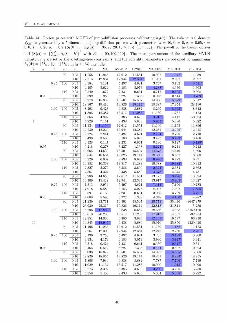
40 J. C. ARISMENDI
Table 14: Option prices with MGEE of jump-diffusion processes calibrating h4(σ). The risk-neutral densityfX(t) is generated by a 5-dimensional jump-diffusion process with parameters λ = 10, δi = 0, νi = 0.05, r =0.10, t = 0.25, σi = 0.2, (S1(0), . . . , S5(0)) = (35, 25, 20, 15, 5), i ∈ 1, . . . , 5. The payoff of the basket option
is Π(S(t)) =(∑5
i=1 Si(t)−K)+
with K ∈ 90, 100, 110. The mean parameters of the auxiliary MVLNdensity gS(t) are set by the arbitrage-free constraints, and the volatility parameters are obtained by minimisingh4(σ) = ∥Ml1,l2∥2 + ∥Ml1,l2,l3∥2 + ∥Ml1,l2,l3,l3∥2.
λ ν t K r J-D MC AV2012 Li2010 MGEE2 MGEE3 MGEE4
90 0.05 11.256 11.945 12.612 11.551 10.937 11.072∗ 11.0390.10 12.315 12.884 12.944 12.384∗ 11.961 12.097 12.027
0.25 100 0.05 3.384 5.181 5.497 4.621 3.747 3.732 3.511∗
0.10 4.105 5.624 6.183 5.073 4.288∗ 4.330 3.303110 0.05 0.540 1.672 2.231 0.661 0.717 0.605∗ 0.608
0.20 0.10 0.699 1.983 3.227 1.338 0.926 0.814 0.789∗
90 0.05 15.273 15.939 16.501 15.507 14.980 15.079∗ 15.8120.10 18.967 19.416 19.826 19.114∗ 18.387 17.954 28.796
1.00 100 0.05 8.293 9.423 9.838 8.682 8.269 8.303∗ 8.3420.10 11.395 12.387 13.517 11.283∗ 11.189 11.267 11.173
110 0.05 3.865 4.992 6.386 3.690 3.913∗ 4.117 -0.3241 0.10 5.920 7.151 9.438 5.680 5.941∗ 5.880 5.822
90 0.05 11.134 11.150∗ 12.612 11.551 11.160 11.153 11.8960.10 12.230 12.229 12.944 12.384 12.231 12.229∗ 12.218
0.25 100 0.05 2.724 2.841 5.497 4.621 2.724∗ 2.726 2.7100.10 3.498 3.563 6.183 5.073 3.493 3.499∗ 3.466
110 0.05 0.128 0.147 2.231 0.661 0.130 0.127 0.128∗
0.05 0.10 0.218 0.278 3.227 1.338 0.224∗ 0.211 0.24290 0.05 14.665 14.630 16.501 15.507 14.678∗ 14.640 14.596
0.10 18.644 18.634 19.826 19.114 18.650∗ 18.637 18.5881.00 100 0.05 6.926 6.907 9.838 8.682 6.926∗ 6.922 6.971
0.10 10.382 10.363 13.517 11.283 10.388 10.382∗ 10.412110 0.05 2.327 2.279 6.386 3.690 2.324∗ 2.334 2.362
0.10 4.367 4.324 9.438 5.680 4.373∗ 4.375 4.43190 0.05 13.288 14.658 12.612 11.551 13.123 13.226∗ 13.094
0.10 14.106 15.422 12.944 12.384 13.917 13.965∗ 13.6270.25 100 0.05 7.313 8.954 5.497 4.621 7.414∗ 7.190 10.785
0.10 7.918 9.580 6.183 5.073 8.047 7.992 7.855∗
110 0.05 3.691 5.169 2.231 0.661 3.988 3.799 3.721∗
0.20 0.10 4.068 5.596 3.227 1.338 4.348 4.160∗ 4.28290 0.05 21.339 22.711 16.501 15.507 20.773∗ 85.440 -3647.379
0.10 23.930 25.319 19.826 19.114 22.813∗ 21.811 5.2801.00 100 0.05 16.296 17.860∗ 9.838 8.682 18.666 4.958 -3159.170
0.10 18.613 20.208 13.517 11.283 17.913∗ 14.867 -32.034110 0.05 12.351 14.063 6.386 3.690 12.133∗ 19.587 96.810
10 0.10 14.345 15.945∗ 9.438 5.680 15.976 -35.850 2229.62090 0.05 11.196 11.236 12.612 11.551 11.169 11.182∗ 11.173
0.10 12.267 12.300 12.944 12.384 12.247 12.260 12.261∗
0.25 100 0.05 3.196 3.253 5.497 4.621 3.205 3.199∗ 3.9000.10 3.934 4.179 6.183 5.073 3.930 3.937∗ 3.941
110 0.05 0.318 0.424 2.231 0.661 0.330 0.317∗ 0.3110.05 0.10 0.465 0.512 3.227 1.338 0.484∗ 0.492 0.523
90 0.05 15.033 15.079 16.501 15.507 14.997 15.035∗ 15.0080.10 18.829 18.855 19.826 19.114 18.801 18.834∗ 18.855
1.00 100 0.05 7.806 7.930 9.838 8.682 7.787 7.796∗ 7.7190.10 11.029 11.134 13.517 11.283 10.990 11.015∗ 10.990
110 0.05 3.273 3.392 6.386 3.690 3.280∗ 3.256 3.2300.10 5.358 5.466 9.438 5.680 5.334 5.338∗ 5.222
40

A MULTI-ASSET OPTION APPROXIMATION 41
Table 15: Percentage of the Monte Carlo simulated paths that are evaluated with the MGEE density andgenerate positive value. The columns Uncalibrated, (h2(σ),MGEE2), (h3(σ),MGEE3) and (h4(σ),MGEE4)correspond to the percentage of the 20,000,000 simulation paths that have positive values when they are evalu-ated under the MGEE density, of Tables 9, 12, 13, and 14, respectively.
λ ν t r Uncalibrated (h2(σ),MGEE2) (h3(σ),MGEE3) (h4(σ),MGEE4)
0.25 0.05 0.6008 1.0000 0.9589 0.74390.20 0.10 0.5999 1.0000 0.9561 0.9299
1.00 0.05 0.5526 1.0000 0.9649 0.55911 0.10 0.5505 1.0000 0.9666 0.7609
0.25 0.05 0.9672 1.0000 0.9996 0.97650.05 0.10 0.9951 1.0000 1.0000 0.9860
1.00 0.05 0.9964 1.0000 1.0000 0.99680.10 0.9976 1.0000 0.9977 0.7141
0.25 0.05 0.9369 1.0000 0.9580 0.91530.20 0.10 0.9379 1.0000 0.9569 0.9152
1.00 0.05 0.8863 1.0000 0.9857 0.909110 0.10 0.8865 1.0000 0.9584 0.8889
0.25 0.05 0.8496 1.0000 0.9983 0.60520.05 0.10 0.8724 1.0000 0.9998 0.7572
1.00 0.05 0.6597 1.0000 0.9967 0.99390.10 0.6642 1.0000 0.9992 0.9936
41


![Stochastic Successive Convex Approximation for …arXiv:1908.11015v1 [cs.IT] 29 Aug 2019 Stochastic Successive Convex Approximation for General Stochastic Optimization Problems with](https://static.fdocuments.us/doc/165x107/5f41e34ca12ac52e26340b0b/stochastic-successive-convex-approximation-for-arxiv190811015v1-csit-29-aug.jpg)


