A Modified Harmony Search Algorithm for the Optimum Design ... · ORIGINAL PAPER A Modiﬁed...

ORIGINAL PAPER

A Modified Harmony Search Algorithm for the Optimum Designof Earth Walls Reinforced with Non-uniform Geosynthetic Layers

Mohammad Motalleb Nejad1 • Kalehiwot Nega Manahiloh1

Received: 2 September 2015 / Accepted: 26 October 2015 / Published online: 26 November 2015

� Springer International Publishing Switzerland 2015

Abstract Traditional design and construction of rein-

forced earth walls assumes uniform length and spacing of

reinforcements. Even though the assumption simplifies the

design and construction efforts, the inherently conservative

approaches followed in picking the final values for the

reinforcement length and spacing result in unnecessarily

big construction costs. This paper presents an improved

harmony search-based approach that can be adopted to

optimize the design of Geosynthetic-reinforced earth walls.

An existing improved harmony search algorithm is modi-

fied into a new harmony search algorithm by extending its

capabilities to consider permutation-based operations for

inter-dependent variables. The involved optimization pro-

cedures are discussed in a step-wise approach. This novel

approach allows the consideration of non-uniform length

and spacing for the reinforcement layers. As such, length of

the Geosynthetic reinforcement and the spacing between

adjacent Geosynthetic layers are taken as the design vari-

ables to be manipulated until the cost of construction is

optimized. Static and dynamic loads are considered. the

application of the proposed optimization technique is

demonstrated on Geosynthetic-reinforced earth walls of

height 5, 7 and 9 m. The extent of cost saving is assessed

by comparing the results of this work and previous work.

The previous work selected for comparison uses harmony

search algorithm to optimize the design and construction of

Earth Walls reinforced with uniform length- and spacing-

Geosynthetic layers. The IHS-based optimization resulted

in Cost reduction of up to 11 %.

Keywords Geosynthetics � Reinforced earth walls �Metaheuristic � Improved harmony search algorithm

(IHSA) � Optimization � Pitch adjustment rate (PAR) �Harmony consideration rate (HCR)

Introduction

Retaining walls are among the most extensively used

structural elements in the construction industry [1]. In spite

of their ubiquitousness, applicability of non-reinforced

retaining walls is confined to lower heights [2]. To over-

come this limitation and enhance the performance of walls

at higher heights, different types of reinforcing material

were introduced. The tension-resisting element (i.e. the

reinforcement) in reinforced earth wall systems works as a

unit with surrounding soil to augment its strength and

sustainability. One group of such reinforcements consists

of different types of Geosynthetics. Geosynthetic rein-

forcements are fabricated from polymeric material. In

reinforced earth systems, the Geosynthetic element plays

the combined pivotal roles of isolation, increased tensile

resistance and improved drainage. Use of Geosynthetics as

reinforcement provides additional strength against various

failure mechanisms. This in turn allows increasing the

reinforced-wall height without the need for external lateral

support (e.g. heavy gravity walls constructed by substantial

concrete material [3]). The decent endurance of the poly-

meric material against erosion has made it a better choice

in reinforcing earth structures [4]. These overlapping

benefits have made Geosynthetic-reinforced walls favor-

able and their design and implementation is expanding.

Over the past five decades the production and use of

polymer-based reinforcement has shown a sustained

upsurge. Geosynthetic reinforced soil walls, compared to

& Mohammad Motalleb Nejad

[email protected]

1 Civil and Environmental Engineering, University of

Delaware, 301 DuPont Hall, Newark, DE 19711, USA

123

Int. J. of Geosynth. and Ground Eng. (2015) 1:36

DOI 10.1007/s40891-015-0039-x

http://crossmark.crossref.org/dialog/?doi=10.1007/s40891-015-0039-x&domain=pdf

http://crossmark.crossref.org/dialog/?doi=10.1007/s40891-015-0039-x&domain=pdf

the classic rigid-walls, have superior flexibility which

makes them better in withstanding natural disasters such as

earthquakes and landslides [3].

In addition to aforementioned benefits, in Geosynthetic-

reinforced soil walls, the cost of the construction is sig-

nificantly lower than other earth retaining systems [5].

Construction cost is one of the decisive factors in the

execution of engineering projects. Koerner and Soong [6]

compared the cost of construction for different types of

retaining walls and showed that the cost of construction for

Geosynthetic-reinforced soil walls is by far lower than its

classic competitors.

In recent studies, harmony search algorithm (HSA) has

been applied in various engineering optimization problems.

River flood models [7, 8], optimal rainfall-runoff models

[9], a design of water distribution networks [10], a simul-

taneous determination of aquifer parameters and zone

structures [11] are some applications of HSA in the Civil

Engineering discipline. HSA has also been applied in

scheduling problems [12], steel frame designs [13], relia-

bility optimizations [14], optimal design of planar and

space trusses and the optimal mass and conductivity design

of a satellite heat pipe [15, 16]. Other studies that make use

of HSA include: transport energy modeling problem [17],

selecting and scaling real ground motion records [18], a

water–water energetic reactor core pattern enhancement

[19], solving machining optimization problems [20], pres-

surized water reactor core optimization [21].

Compared to other metaheuristic methods HSA pos-

sesses unique features in that it: considers all the solution

harmonies during new iterations; and utilizes stochastic

random searches. These features enable HSA to, system-

atically, handle huge optimization problems with less

mathematical requirements [22] and make it a preferable

tool in optimization-related research.

Recently, different methods (i.e. Particle Swarm Opti-

mization (PSO), Ant Colony etc.) have been combined

with HSA in pursuit of improved hybrid-algorithms [23,

24]. Several other studies have also tried to further improve

the performance of HSA. Wang and lee [25] proposed a

differential harmony search algorithm in solving non-con-

vex economic load dispatch problems. An improved har-

mony search (IHS) [22] and a global-best harmony search

(GHS) [26] algorithms have been implemented to enhance

the searching power of the HSA.

Basudhar et al. [27] optimized Geosynthetic-reinforced

walls using Sequential Unconstrained Minimization Tech-

nique (SUMT algorithm). Using HSA, and assuming the

constant-length and number of Geosynthetic layers as

design variables and construction cost as the objective

function, Manahiloh et al. optimized the design of

Geosynthetic-reinforced walls [1]. In both studies the

length of reinforcement and the spacing between adjacent

layers were set to be constant.

In this study the applicability of IHS is discussed and its

utilization is demonstrated by optimizing the design and

construction of Geosynthetic-reinforced Earth Walls. The

algorithm associated with IHS is modified and expanded to

account for non-uniform length of Geosynthetic rein-

forcement layers and non-constant spacing between adja-

cent layers. The optimization variables are: the

independent lengths of Geosynthetic in each layer; and a

vector that contains distance information between two

adjacent Geosynthetic layers.

Analysis of Geosynthetic-Reinforced Earth Wall

Stability analysis for Geosynthetic-reinforced walls intro-

duced in FHWA code [28] uses Rankine’s theory. The

same theory is adopted in this study to analyze walls while

non-uniform variation in spacing and length of geosyn-

thetic reinforcement is permitted. The non-uniform length

and spacing values are set to be picked with a random

selection process pre-defined in the HSA. The feasibility of

construction is accounted for by constraining the variation

in length of geosynthetics in such a way that it shows a

consistent trend. Moreover, the length of geosynthetics in

each layer is kept lower than the smaller of: the maximum

limit of the range for length; and the length of geosynthetic

in the layer above. Stability analyses, for Geosynthetic-

reinforced walls with a vertical face, are made assuming a

rigid body behavior for the reinforced zone as shown in

Fig. 1. Lateral earth pressures are computed on a vertical

surface located at the end of the reinforced zone. The

reinforced zone is further divided into multiple sub-zones.

The first zone related to shortest length of the reinforce-

ment which is associated with the bottom layer of

Geosynthetics. The other zones are fractions of an assumed

rigid body that exceed the area corresponding to the least

length. Parameters used in the design process are presented

in Fig. 1.

For horizontal and inclined backfill (angle b from hor-

izontal) retained by a smooth veritcal wall, the coefficient

of active lateral earth pressure may be calculated from

Eqs. (1) and (2) respectively.

Ka ¼ tan2 45� /2

� �ð1Þ

Ka ¼ cos b� cos b�ffiffiffiffiffiffiffiffiffiffiffiffiffiffiffiffiffiffiffiffiffiffiffiffiffiffiffiffiffifficos2 b� cos2 /

pcos bþ

ffiffiffiffiffiffiffiffiffiffiffiffiffiffiffiffiffiffiffiffiffiffiffiffiffiffiffiffiffifficos2 b� cos2 /

p ð2Þ

In this study the active earth pressure coefficient (Ka) for

the backfill is designated with Kae. / is defined as /b and

/f, for the soil in reinforced zone and the retained soil (i.e.

36 of 15 Int. J. of Geosynth. and Ground Eng. (2015) 1:36

123

soil behind and on the top of the reinforced mass)

respectively.

Regardless of type of reinforcement, any reinforced sys-

tem should be checked for internal and external stability. The

internal stability deals with interactions between reinforce-

ments and the material in contact with them andmechanisms

that lead to soil fracture and the associated rupture of the

reinforcements. The external stability, on the other hand,

deals with the behavior of the rigid body of reinforced-soil

zone interacting with neighboring soil and the mechanisms

that disturb its stability. The design of geosynthetic-rein-

forced soil walls is not considered safe until the safety factors

against internal and external failure mechanisms are above

the corresponding minimum values specified by codes.

Internal stability analysis of non-uniform lengths and

spacing is exactly the same as that of uniform lengths and

spacing. Details regarding this have been covered in other

literature [1, 28].

Generally, three failure mechanisms are assessed in

examining the external stability of retaining structures. In

geosynthetic-reinforced earth wall systems, the sliding of the

rigid body of reinforced-soil system, bearing capacity of the

foundation soil below the reinforced zone and overturning of

the reinforced-soil zone are considered to be these three

failure mechanisms. Figure 1 shows the external forces in a

geosynthetic-reinforced wall system. In the figure, Vi refers

to the weight of the soil enclosed by the associated geometric

shapes. The summation of the weights Vrec, Vq and V1

through VNoG-1, is the total weight of the soil within the

reinforced zone where NoG refers to the number of

geosynthetic layers. Considering the reinforced system as a

plane-strain problem, this weight is considered to act as a

block. Since the wall embedment depth is small, the stabi-

lizing effect of the passive pressure (moment) has been

neglected in the analysis. The factors of safety against the

above failure mechanisms are presented below.

• Safety factor against overturning It is assumed that, if

overturning takes place, the whole reinforced zone will

behave as a rigid body. Referring to Fig. 1, the safety

factor against overturning is evaluated by considering

moment equilibrium about point O. It can be calculated

from:

whereP

MRo andP

Mo are the resisting and overturn-

ing moments respectively. The other parameters in Eq. 3

are as defined and indicted in Fig. 1.

• Safety factor against sliding Three relevant components

are accounted for during the evaluation of safety

against sliding. The first consists of the weight of the

reinforced zone and all vertical forces acting above this

zone. Interface friction angle between the soil and

fabric, d, is the second component that needs consid-

eration. The third components refers to all the driving

FSoverturning ¼P

MRoPMo

¼ FT1 � ðh=3Þ þ FT2 � ðh=2Þð Þ cos bð Þ

Vrec � ðlmin=2Þ þ Vq � ð2lmax=3Þ þPNoG�1i¼1

Vi � liþlmin

2

� �þ qs � ðl2max=2Þ

ð3Þ

Fig. 1 Parameters used in

different steps of the design and

external forces considered for

the Geosynthetic reinforced

retaining wall system

Int. J. of Geosynth. and Ground Eng. (2015) 1:36 of 15 36

123

lateral forces that try to cause sliding. The factor of

safety against sliding can be expressed as:

FSsliding ¼P

horizontal resisting forcesPhorizontal driving forces

¼P

PRPPd

¼Vrec þ Vq þ

PNoG�1i¼1

Vi þ qs � lmax

� �� tan d

FT1 þ FT2ð Þ cos bð Þ

ð4Þ

whereP

PR andP

Pd are resisting and driving forces

respectively.

• Safety factor for bearing capacity: The reaction’s

eccentricity, e, from the centerline of the reinforced

earth block, can be evaluated from moment equilibrium

about point A:

e ¼P

Md �P

MRPV

ð5Þ

In this study Meyerhof’s equivalent-rectangular pressure

distribution [29, 30] is used to calculate the bearing

capacity of the foundation soil under eccentric load con-

ditions. To stay in the conservative side of design, lmin is

used in calculating the vertical stress acting on the foun-

dation. For mild natural ground slopes (i.e. small angels of

b in Fig. 1), the vertical pressure rv can be calculated usingthe following equation:

rv ¼ Vrec þ Vq þXNoG�1i¼1

Vi

!,lmin � 2eð Þ ð6Þ

Using the Terzaghi’s equation [31] for a strip footing on

a cohesionless soil and assuming q as the surcharge asso-

ciated with the soil to the left of the reinforced-soil, the

ultimate bearing capacity can be calculated as:

qult ¼ qNq þ 0:5cfNf lmin ð7Þ

The safety factor for bearing capacity is then obtained

from:

FSbear ¼qult

rvð8Þ

In the evaluation of external stability for a wall under

dynamic conditions, in addition to the static forces, the

inertial force and half of the dynamic soil thrust are

assumed to act on the wall [28]. The details for dynamic

considerations can be referred from earlier works [1, 32].

Objective Function

Mathematical Formulation

In this study the cost of construction is taken as the

objective function and is minimized by searching for a set

of optimum design variables. The rates associated with

various items (i.e. the cost factors) are presented in

Table 1. For comparison purposes, the same cost parame-

ters, to that of Manahiloh et al. [1] have been adopted.

The total amount attained by the objective function, in

terms of the length and spacing between the geosynthetic

reinforcements (i.e. the design variables), is obtained by

summing all the costs listed above.

Design Constraints

The design constraints, applied to check the stability of the

reinforced earth-wall and corresponding minimum recom-

mended safety factors, have been presented by Manahiloh

et al. [1]. In addition to six constraints applied for the case of

uniform lengths and spacing described by Manahiloh et al.

[1], a new constraint is needed to consider the feasibility of

construction. Accounting for the process of excavation

which imposes a restriction that confine the length of each

geosynthetic to be lower than that of the adjacent upper

layer, we can introduce the following constraint:

g7 ¼ lnþ1 � ln\0 for n ¼ f1; 2; . . .; NoG� 1g ð9Þ

Table 1 Assumed cost factors (after Manahiloh et al. [1])

Item Assumed cost factor Cost applied per unit

length of the wallSymbol Value

Geogrid Geotextile

Leveling pad C1 $10/m $10/m c1

Wall fill C2 $3/1000 kg $3/1000 kg c2 � cfg� ðVolreinforced zoneÞ

Geosynthetic C3 $[Ta(0.03) ? 2.0]m2 $[Ta(0.03) ? 2.6]m2 PNoGi¼1

c3 � li

MCU face unit* C4 $60/m2 0 c1 9 H

Engineering tests C5 $10/m2 $30/m2 c5 9 H

Installation C6 $50/m2 $50/m2 c6 9 H

* The Modular Concrete Facing Units (MCU) are only applied for Geogrid type walls


123

Applying Design Constraints to the Objective

Function

For the sake of simplicity, a linear penalty function has

been used in this study. The mathematical formulation for

an objective function subject to seven constraints can be

expressed as follows:

min f ðxÞ subject to gj� 0; j ¼ 1; 2; . . .; 7 ð10Þ

The modified objective function /(x) can then be rep-

resented by:

/ðxÞ ¼ f ðxÞ½1þ K � C� ð11Þ

where K and C are penalty parameters in which K is a con-

stant coefficient which increases the rate of penalty applied

to the function and for most engineering problemsK = 10 is

assumed appropriate. C is a measure of violation defined as:

C ¼Xmj¼1

Cj Cj ¼ gj if gj [ 0

Cj ¼ 0 if gj� 0

�ð12Þ

Design Variables

In traditional HSA, the variables are independent. Using

each spacing, as an individual variable, results in a conflict

during algorithm execution. Noting that the summation of

all spacing values must be equal to the height of the wall,

the algorithm conflict can systematically be avoided by

introducing an additional constraint that restricts the

summation of all spacing values to be equal to the height

of the wall. However, it has been discovered that this

method introduces additional computational effort. To

overcome this difficulty, a vector that contains all the

distances (dn) between consecutive geosynthetic layers is

considered in each harmony as a single variable (S) as

shown in Eq. (13).

S ¼ d1;d2 � � � dn � � � dNoGþ1½ � ð13Þ

The allocation of each value in this vector depends on the

discretization of the acceptable range for spacing. It is also

dependent on the algorithm’s capability to search for com-

binations of spacing values whose summation equals to the

height of the wall. The details are provided in the next sec-

tions.The other variables are the lengths of geosynthetic in

each layer staring from top of the wall. Each harmony,

therefore, consists of a vector of dependent variables for

spacing and lengths of each layer as independent variables as

shown in Eq. (14).

H ¼ S l1 l2 � � � ln�1 lnjC½ � ð14Þ

In the calculation for spacing values between adjacent

layers of geosynthetic layers, the spacing associated with

each layer is assumed as the average of distances above and

below each layer. This assumption is indicated in Eq. (15).

Sn ¼dn þ dnþ1

2ð15Þ

This value is modified for the first and last layers of

geosynthetics to account for absence of adjacent layer of

geosynthetics above and below those layers respectively.

Implementation of Harmony Search Algorithm

The process of finding a pleasing and ear-catching harmony

in music is analogous to finding the optimality in an opti-

mization process [33]. HSA is known as one of the powerful

metaheuristic optimization methods inspired by improvisa-

tion ability of musicians that involves less mathematical

efforts and highly accurate results. The base structure of this

algorithm has been presented by Geem [34]. Since then,

efforts have been made to modify the functionality of the

base algorithm. In this study an improved harmony search,

proposed by Mahdavi et al. [22], is extended and imple-

mented to the optimization of the cost associated with the

construction of geosynthetic-reinforced earth walls.

The steps involved in the IHS are presented in the

flowchart shown in Fig. 2. As indicated in the flowchart, the

optimization program is initiated with a set of random har-

monies (also called solution vectors or individuals) stored in a

matrix called harmony memory (HM). The term ‘‘harmony’’

refers to solution vectors that contain sets of decisionvariables.

HS algorithms use three mechanisms to produce a new har-

mony: memory consideration, random choosing, and pitch

adjustment. The basicHS algorithmuses a constant probability

and a fixed value to pitch-adjust the variables inside the new

harmonies. IHS, on the other hand, employs interactive func-

tions to improve the convergence of the harmonies to the

optimized solution. In each step, every new solution that is

better than any of the stored harmonies from previous steps

takes the place of the worst solution in the HM until termina-

tion criteria is satisfied. In order to fit the dependent variables

into the HM and assign a random neighborhood for them, a

new procedure is developed as discussed below.

Step 1: Introduction of the Optimization Program

and Parameters for the Algorithm

In this step, a set of specific parameters is introduced to the

IHSA. Some of the parameters are:

i. The harmony memory size (HMS). This determines

the number of individuals (solution vectors) in the

HM. For a given wall, in this work, 10 solution

vectors are introduced to build the harmony memory.


123

ii. The harmony memory consideration rate (HMCR).

This parameter is utilized while decision is made to

choose new variables from the HM or to assign new

arbitrary values.

iii. The pitch adjustment rate (PAR). PAR, increasing

functionally with iteration, is used to decide the

adjustments of some decision variables selected

from memory. The IHSA expects the definition of

minimum and maximum PAR values to this function.

iv. The bandwidth function (BW). This function determines

the range of the adjustment that occurs to the variables in

each iteration. A set of minimum and maximum band-

width values (BWmin and BWmax) must be introduced to

this function. The value of this function decreases from

BWmax in first iteration to BWmin in last iteration.

v. The maximum number of iteration (NI) which is also

called Stopping or Termination Criteria.

vi. The permutation evaluation rate (PER). This param-

eter is useful in deciding whether different permuta-

tions of the solution vector, holding information about

the non-uniform geosynthetic spacing values, are

considered or not. This parameter is not included in

the traditional HSA and HIS. It is proposed, by this

work, in order to increase the probability of consider-

ing rare occurrences for vector S and to evaluate its

different permutations.

The values attained by the parameters HMCR, PARmin,

PARmax, BWmin, BWmax and HMS differ from one problem

to another and can affect the convergence of the HSA to the

optimum solution. Lower values attained by the PAR indi-

cate an increased chance of adjusting one parameter without

changing the others. However, BW must take bigger values

for the first few iterations in order to ensure the creation of

diversified solution vectors by the algorithm [22]. Setting

appropriate values for these parameters will also enable the

algorithm to avoid getting trapped in a local optimum. Lee

et al. [16] proposed a value between 0.7 and 0.95 for

HMCR; 0.2 and 0.5 for PAR; and 10 and 50 for HMS to

achieve a good performance in the traditional HSA. In IHS

Algorithm the value of PAR and BW varies with progressive

iterations [22].

The optimization problem is initially presented as min-

imizing FðS; l1; l2; . . .; lNÞ which is the objective function.

The vector S and geosynthetic lengths are the decision

variables where S ¼ d1;d2 � � � dn;dNoGþ1½ � and

l ¼ lN jN ¼ 1; 2; . . .;NoGf g. Therefore, the number of

decision variables (NoV) is equal to the number of

geosynthetic layers plus one (i.e. Eq. (16). Each length

value is an independent variable which is represented by its

layer number and the additional variable S is an array made

up of the inter-dependent spacing values.

NoV ¼ NoGþ 1 ð16Þ

In this paper the lower and upper bounds for the decision

variables of type l (i.e. reinforcement length) are set to 1 m

and 10 m respectively. Applying the terms upper and lower

bound for the array S does not make a clear sense as

S contains a set of inter-dependent spacing-related vari-

ables (d). However, the lower and upper bounds for the

dependent variables can be defined. The minimum and

maximum values for the individual spacing values are

considered to be 0.2 m and 1.5 m, respectively. These

Fig. 2 IHS Algorithm

flowchart


123

numbers were picked to be consistent, for result compar-

ison purposes, with Manahiloh et al. [1]. In addition, these

limit values can be applied to d-values so that the spacing

values are allowed to vary within a specified range.

One of the challenging tasks, faced in this study, was how

to assign the inter-dependent d values and form an optimized

vector S. One way this task could be accomplished is by

combining the gradient descentmethodwithHarmonySearch

Algorithm and finding the optimum value of the S vector.

Another, yet simpler, way is to discretize the domain of d into

a few finite values and design a probabilistic method to find

the optimum vector S. In the later approach, any possible

combination of the discretized values of the domain—with a

fixed summation equaling to the height of thewall—will have

an equal probability of being chosen to make up the vector S.

To elaborate on this, let’s assume that the continuous range of

d values (i.e. [0.2, 1.5]) is to be discretized into a certain

number of distances (i.e. NoD). This way, the difference

between each discretized value in the given range is kept

constant and less than a specified value. In this paper, DV

refers to this value and the NoD is then given as:

NoD ¼ Smax � Smin þ DV

DV

�� ð17Þ

The exact value of the difference between each dis-

cretized value within the domain is found by dividing the

range by NoD. Once calculated, the discretized values are

set in a vector. A random combination of the NoG ? 1

number of the discretized values—with a fixed summation

equaling to the height of the wall—can be assumed as a

possible solution for the vector S.

The values for the length of geosynthetic layers (i.e. l val-

ues) are independently selected with a stochastic process. The

ranges fromwhich the algorithmpicksvalues for theNoG and l

values are set based on experience and validated literature.

Step 2: Initialization of Initial Harmony Memory

(HM)

In this step, the initial HM matrix is populated with as

many randomly generated individuals as the HMS and the

corresponding Objective Function value of each set of

random individuals FðS; l1; l2; . . .; lNÞ. The initial harmony

memory is formed as follows:

ð18Þ

After the variables are assigned, the IHS algorithm

solves the problem such that the Objective Function is

optimized by minimizing its value. Upon the process of

optimization, to minimize the Objective Function, Cost

values associated with each set of individuals are arranged

in a numerically ascending order.

Step 3: Improvisation for a New Harmony

In this step, a New Harmony vector F0ðS0; l01; l02; . . .; l0NÞ, isimprovised based on four mechanisms: (1) Memory Con-

sideration; (2) Random Selection; (3) Pitch Adjustment;

and (4) Permutation evaluation.

Harmony Memory Consideration

HMCR and 1-HMCR are defined as the rate of choosing

one value from previously stored values in HM and the rate

of randomly selecting one value from the possible range for

variables respectively. For the ith iteration and the jth

variable in each harmony vector we can write the

following:

For j ¼ 1 :

S0i S0i 2 S1;S2; . . .;SHMS

with probability HMCR

S0 2 A new combination of H with probability (1-HMCR)

(

ð19Þ

For j [ 1 :

l0ij l0ij 2 l1j ; l

2j ; . . .; l

HMSj

n owith probability HMCR

l0i 2 lmin; lmax½ � with probability (1-HMCR)

(

ð20Þ

For an instance, assuming HMCR equal to 0.95, HSA

selects the new variables from values stored in HM with a

probability of 95 %.

Pitch Adjustment

In this step, each decision variable associated with the new

individual is pitch-adjusted with a probability that was

assigned to that variable. The main difference between

HSA and IHS is observed when the pitch adjustment rate

(PAR) is assigned to each variable in each step. In IHS a

lower and upper level is defined for PAR. With progressive

iterations, PAR linearly changes from low to high values.

Variation of PAR with iteration in IHS was expressed by

Mahdavi et al. [22] as:

PARi ¼ PARmin þPARmax � PARmin

NI� i ð21Þ

where i is the iteration number and NI is the maximum

number of iterations as defined previously. The justification


123

for this linear relationship was that small PAR values sig-

nificantly increase the number of iterations [22]. However,

small PAR values are essential in first iterations to prevent

the algorithm from being trapped in local optimums.

IHS bases itself on the dynamic interaction between

PAR and BW. This dynamic interaction is manifest as the

magnitude (distance) of the adjustment made to each

variable, on each harmony, in the Pitch Adjustment oper-

ator. Generating high values of BW during the first itera-

tions helps the algorithm to evaluate higher distances. This

in turn augments the search capability of the algorithm. As

the number of iterations increases, the system examines

closer neighborhoods (distances from the newly obtained

and assigned variables) and optimize their results further.

The values of the BW which are bounded by lower and

upper limits (i.e. BWmin and BWmax), are set to decrease

exponentially from BWmax to BWmin. Mahdavi et al. [22]

proposed the following equation for BW in each iteration:

BWi ¼ BWmax þ exp c� ið Þ ð22Þ

where c is a coefficient given by:

c ¼ln BWmin

BWmax

� �NI

ð23Þ

Pitch Adjustment is applied to two kinds of variables.

These are: (i) A vector of dependent variables (i.e. vector S

made of the spacing values), and (ii) A set of independent

variables (i.e. lengths).

Pitch adjustment for the vector S In this study, the values

of 0.35 and 0.99 are considered for PARmin, PARmax, respec-

tively. Having calculated the PARi, within the range [PARmin,

PARmax], for each iteration from Eq. (21), one can adjust the

values of the vector S with the probability of PARi, as:

Pitch adjusting decision for S0i

Yes With probability PARi

No With probability 1� PARi

�ð24Þ

Two simple methods can be adopted to define neigh-

borhoods for vectors which are made of inter-dependent

individual variables whose summation must remain con-

stant (e.g. Vector S). The first method uses a small noise

vector of the same number of elements and adds these

elements with that of the original vector. Assume that SS?N

is a vector made by summing elements of the random noise

vector (scaled by BW1) and elements of vector S.

SSþN ¼ Sþ BW1i � ða random noise vectorÞ ð25Þ

where BW1i [ [BW1min, BW1max] is distance (neighbor-

hood) bandwidth for vector S and can be calculated from

Eq. (22) for each iteration. BW1i is introduced to the IHS in

order to assist the algorithm pick an optimal path in the

close neighborhoods of vector S. Note that the sum of the

elements of the vector defined in Eq. (25) does not add up

to a value equal to the height of the wall. In order to bring

the summation to a value equaling the height of the wall,

one needs to assess the locus of such vectors which takes

the shape of a hyper-diamond. If the sum of the elements of

SS?N is designated by Vsum, a new pitch adjusted neigh-

borhood for the vector S (i.e. S0

i) located on the hyper-

diamond can be defined as:

S0i ¼ Ss SSþNð Þ=Vsum ð26Þ

where Ss represents the sum of the elements of vector S.

This method, however, does not accommodate for any

definite arrangement and order in framing the neighbor-

hoods. There is an alternative approach that enables the

algorithm to have an arranged set of vectors. In this

method the neighborhoods of a vector can be defined by

adding a set of defined vectors that add a small value to

some elements and subtract it from other elements so as to

keep the summation of the elements fixed. Each row of

the matrix presented below shows some vectors that can

be used to manipulate vector S and produce a new

neighborhood:

Nset ¼

BW1i �BW1i 0 0 0 0 � � �BW1i � 2 �BW1i � 2 0 0 0 0 � � �BW1i � 2 �BW1i �BW1i 0 0 0 � � ��BW1i � 2 BW1i BW1i 0 0 0 � � �BW1i � 3 BW2� 2 BW1i �BW1i �BW1i � 2 �BW1i � 3 � � ��BW1i � 2 �BW1i BW1i BW1i � 2 0 0 � � �

BW1i BW1i �BW1i �BW1i 0 0 � � �... ..

. ... ..

. ... ..

. ...

2666666666664

3777777777775

|fflfflfflfflfflfflfflfflfflfflfflfflfflfflfflfflfflfflfflfflfflfflfflfflfflfflfflfflfflfflfflfflfflfflfflfflfflfflfflfflfflfflfflfflfflfflfflfflfflfflfflfflfflfflfflfflfflfflfflfflfflfflfflfflfflfflfflfflfflfflfflfflfflfflfflfflfflfflfflffl{zfflfflfflfflfflfflfflfflfflfflfflfflfflfflfflfflfflfflfflfflfflfflfflfflfflfflfflfflfflfflfflfflfflfflfflfflfflfflfflfflfflfflfflfflfflfflfflfflfflfflfflfflfflfflfflfflfflfflfflfflfflfflfflfflfflfflfflfflfflfflfflfflfflfflfflfflfflfflfflffl}Number of elements of S

ð27Þ


123

In Eq. (27), each row of Nset is a vector that contains

scaled BW1 values that can be used in defining a neigh-

borhood for vector S. Each row can be added to (or sub-

tracted from) vector S to produce a new neighborhood. All

permutations of the elements in each row of Nset need to be

considered in the calculation in order to have accurate

estimate of the neighborhood vectors. Similar to the first

method discussed above, this approach assigns values for

BW1i within a range bounded by a minimum and maxi-

mum. In this study the lower and upper limits for BW1 are

set to 0.009 and 0.2 respectively. These boundary values

are set to attain an increased accuracy while running iter-

ations for the spacing values that add up to give the height

of the wall. Using the second approach, a set of random

neighborhoods for the vector S can be generated using the

following equation.

S0i ¼ Sþ Nset ð28Þ

In this paper, all close neighborhoods are: generated

using the second method; evaluated with the probability of

PARi; and stored in a matrix ready to be evaluated with

other adjusted harmonies.

Pitch adjustment for lN The values of PARmin and

PARmax are the same for independent variables (lengths).

Pitch adjustment for the lengths is done with the proba-

bility of PARi:

Pitch adjusting decision for l0i

Yes With probability PARi

No With probability 1� PARi

�ð29Þ

The lengths are modified to their neighboring values

with the probability of PAR1. For the problem discussed in

this paper, Pitch Adjustment is applied for length (li) as

described by the following expression:

l0i ¼ l0i � ða random valueÞ � BW2i ð30Þ

where BW2i for each step is calculated from Eq. (22). The

values of BW2 min and BW2max are given by Eq. (31).

BW2min ¼ 0:009

BW2max ¼ 0:05� ðlmax � lminÞð31Þ

where lmin and lmax are the lower and upper limits for the

range defined for lengths of geosynthetics which are equal

to 1 and 10 m, respectively. The random value in Eq. (30)

is determined using the Gaussian Membership Function

which covers a higher range for the random value and gives

a small possibility to higher values to be chosen. If Pitch

Adjustment causes a variable to fall outside the given

range, an alternative value must be replaced for the outlier.

This alternative value can be the minimum or maximum of

the range assigned to the variable.

Permutation Evaluation for the Vector S

In this study, a set of random number of permutations of

the vector S is also evaluated with the probability of PER

to increase the chance of the S vectors that have small

probability of random selection. This evaluation is done

after Pitch Adjustment for the produced S vectors. The

number of these permutations is randomly chosen from 1 to

10.

Step 4: Updating the Harmony Memory

If the newly generated Harmony Vector is better than any

of the stored Harmony Vectors in the HM (i.e. results in a

better Objective Function value than that for the stored

individuals), it will replace the old stored vector in the HM.

Otherwise, the algorithm enters the next loop (iterating

between Steps 3 and 4) without any replacement.

Step 5: Evaluation of the Termination Rule

Steps 3 and 4 continue to repeat until the Termination Rule

is satisfied. The last solution vector that meets the

requirements of the Termination Rule is reported as the

optimized solution for the problem under consideration.

Undoubtedly, the maximum number of generations could

be different from problem to problem depending on the

desired accuracy. In this study, The Termination rule is

considered to be satisfied, when the values of Cost Func-

tion, F, are equal up to ten decimal places for 200 con-

secutive iterations. Figure 3 shows the reduction in cost

with iterations for 9 meter Geogrid-Wrap Wall with

Am = 0 and overburden pressure equal to qs = 10. It can

be seen that the Mean Cost Values in the HM converge to

the best cost, after 300 iterations. Further iteration causes

slight changes in the variables, however, the changes in

cost function will be insignificant.

Fig. 3 Reduction in cost with iterations for 9 meter Geogrid-Wrap

Wall with Am = 0, qs = 10


123

Results and Discussions

As was discussed in Sect. 6, an improved harmony search

(IHS) was modified into a novel searching algorithm by

incorporating a permutation-based optimization technique

to handle non-uniform length and spacing of geosynthetic

reinforcements. The analyses discussed herein and the

associated results were compared to the work by Manahi-

loh et al. [1]. As such, the parameters, system geometry and

load configurations were made, by design, similar to that of

Manahiloh et al. The input parameters used in defining

each problem are presented in Table 2.

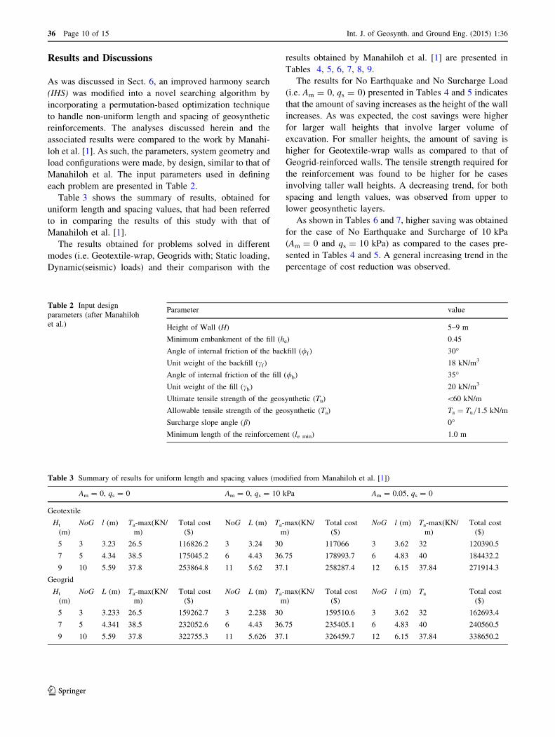
Table 3 shows the summary of results, obtained for

uniform length and spacing values, that had been referred

to in comparing the results of this study with that of

Manahiloh et al. [1].

The results obtained for problems solved in different

modes (i.e. Geotextile-wrap, Geogrids with; Static loading,

Dynamic(seismic) loads) and their comparison with the

results obtained by Manahiloh et al. [1] are presented in

Tables 4, 5, 6, 7, 8, 9.

The results for No Earthquake and No Surcharge Load

(i.e. Am = 0, qs = 0) presented in Tables 4 and 5 indicates

that the amount of saving increases as the height of the wall

increases. As was expected, the cost savings were higher

for larger wall heights that involve larger volume of

excavation. For smaller heights, the amount of saving is

higher for Geotextile-wrap walls as compared to that of

Geogrid-reinforced walls. The tensile strength required for

the reinforcement was found to be higher for he cases

involving taller wall heights. A decreasing trend, for both

spacing and length values, was observed from upper to

lower geosynthetic layers.

As shown in Tables 6 and 7, higher saving was obtained

for the case of No Earthquake and Surcharge of 10 kPa

(Am = 0 and qs = 10 kPa) as compared to the cases pre-

sented in Tables 4 and 5. A general increasing trend in the

percentage of cost reduction was observed.

Table 2 Input design

parameters (after Manahiloh

et al.)

Parameter value

Height of Wall (H) 5–9 m

Minimum embankment of the fill (he) 0.45

Angle of internal friction of the backfill (/f ) 30�Unit weight of the backfill (cf ) 18 kN/m3

Angle of internal friction of the fill (/b) 35�Unit weight of the fill (cb) 20 kN/m3

Ultimate tensile strength of the geosynthetic (Tu) \60 kN/m

Allowable tensile strength of the geosynthetic (Ta) Ta ¼ Tu=1:5 kN/m

Surcharge slope angle (b) 0�Minimum length of the reinforcement (le min) 1.0 m

Table 3 Summary of results for uniform length and spacing values (modified from Manahiloh et al. [1])

Am = 0, qs = 0 Am = 0, qs = 10 kPa Am = 0.05, qs = 0

Geotextile

Ht

(m)

NoG l (m) Ta-max(KN/

m)

Total cost

($)

NoG L (m) Ta-max(KN/

m)

Total cost

($)

NoG l (m) Ta-max(KN/

m)

Total cost

($)

5 3 3.23 26.5 116826.2 3 3.24 30 117066 3 3.62 32 120390.5

7 5 4.34 38.5 175045.2 6 4.43 36.75 178993.7 6 4.83 40 184432.2

9 10 5.59 37.8 253864.8 11 5.62 37.1 258287.4 12 6.15 37.84 271914.3

Geogrid

Ht

(m)


m)

Total cost

($)


m)

Total cost

($)

NoG l (m) Ta Total cost

($)

5 3 3.233 26.5 159262.7 3 2.238 30 159510.6 3 3.62 32 162693.4

7 5 4.341 38.5 232052.6 6 4.43 36.75 235405.1 6 4.83 40 240560.5

9 10 5.59 37.8 322755.3 11 5.626 37.1 326459.7 12 6.15 37.84 338650.2


123

Table 4 Optimum design values for Geotextile-wrap walls Am = 0, qs = 0

Ht (m) Ta-max (kN/m) lmin lmax Cost ($) Saving with respect to equal lengths and spacings (%)

5 36.5 1 m 10 m 113705.6 2.67

Lengths l1 l2 l3 l4 Distances d1 d2 d3 d4 d5

4.62 2.04 1.26 1.11 1.5 1.5 1.5 0.29 0.21


7 55.86 1 m 10 m 166944.58 4.62

Lengths l1 l2 l3 l4 l5 Distances d1 d2 d3 d4 d5 d6

7.97 3.1 2.3 1.5 1.11 1.5 1.5 1.5 1.5 0.79 0.21


9 60 1 m 10 m 229028.5 9.8

Lengths l1 l2 l3 l4 l5 l6 l7 Distances d1 d2 d3 d4 d5 d6 d7 d8

10 6.7 4.1 2.6 2.1 1.5 1.2 1.5 1.5 1.5 1.5 0.96 1.15 0.53 0.35

Table 5 Optimum design values for Geogrid-reinforced walls Am = 0, qs = 0

Ht (m) Ta-max (kN/m) lmin lmax Cost($) Saving with respect to equal lengths and spacings (%)

5 36.5 1 m 10 m 156217.1 1.91


4.62 2.04 1.26 1.11 1.5 1.5 1.5 0.3 0.2


7 54.8 1 m 10 m 225120.5 2.98

Lengths l1 l2 l3 l4 l5 l6 Distances d1 d2 d3 d4 d5 d6 d7

8 3.1 2.3 1.5 1.2 1.1 1.5 1.5 1.5 1.5 0.59 0.21 0.2


9 59.9 1 m 10 m 301860.6 6.47

Lengths l1 l2 l3 l4 l5 l6 l7 l8 Distances d1 d2 d3 d4 d5 d6 d7 d8 d9

10 6.7 4 2.66 2.11 1.65 1.3 1.16 1.5 1.5 1.5 1.47 1 1 0.6 0.2 0.23

Table 6 Optimum design values for Geotextile-wrap walls Am = 0, qs = 10 kPa

Ht (m) Ta-max (kN/m) lmin lmax Cost ($) Saving with respect to uniform lengths and spacing (%)

5 40 1 m 10 m 115006.56 1.76


5.1 2.1 1.38 1.11 1.33 1.49 1.48 0.5 0.2


7 60 1 m 10 m 167738.5 6.29


8.1 3.1 2.3 1.54 1.12 1.49 1.5 1.49 1.47 0.82 0.22


9 60 1 m 10 m 231288.1 10.45


10 7.5 3.49 2.74 2.2 1.59 1.3 1.17 1.5 1.5 1.5 1.4 0.88 1.14 0.54 0.33 0.2


123

Table 7 Optimum design values for Geogrid-reinforced walls Am = 0, qs = 10 kPa


5 39.8 1 m 10 m 157449.7 1.29


5.23 2.2 1.44 1.11 1.2 1.48 1.47 0.63 0.22


7 56.55 1 m 10 m 225458.7 4.22


9.26 3.41 2.63 1.85 1.4 0.88 1.5 1.5 1.5 0.87 0.75


9 59.8 1 m 10 m 303382.37 7.1


9.99 6.49 4.53 2.7 2.23 1.77 1.27 1.16 1.5 1.5 1.5 1.45 0.84 1.02 0.69 0.3 0.2

Table 8 Optimum design values for Geotextile-wrap walls Am = 0.05, qs = 0


5 39.3 1 m 10 m 118560.7 1.52


5.92 2.14 1.27 1.1 1.5 1.5 1.49 0.31 0.2


7 56.55 1 m 10 m 225458.7 4.22


9.53 4.64 2.36 1.54 1.2 1.11 1.5 1.5 1.5 1.5 0.6 0.2 0.2


9 59.9 1 m 10 m 248689.4 8.54


10 9.54 7.2 4.16 2.16 1.76 1.34 1.2 1.48 1.49 1.49 1.14 1.22 0.83 0.89 0.25 0.21

Table 9 Optimum design values for Geogrid-reinforced walls Am = 0.05, qs = 0


5 39.34 1 m 10 m 160904.7 1.1


5.9 2.13 1.26 1.11 1.5 1.5 1.5 0.3 0.2


7 58.16621 1 m 10 m 234729.7 2.42


9.99 3.77 2.49 1.55 1.22 1.12 1.5 1.5 1.5 1.5 0.6 0.2 0.2


9 59.78175 1 m 10 m 319736.72 5.58


10 9.96 6.3 3.74 2.65 1.73 1.58 1.32 1.5 1.5 1.46 1.28 1.05 0.93 0.7 0.22 0.36


123

The total saving in the presence of seismic loads was

found to be lower (Tables 8, 9) compared to the other

modes of analyses. This reduction in total saving can be

related to the extent of seismic load considered in analysis.

The inertial force was assumed to act over a zone of width

equaling half of the wall height. This assumption indeed

leads to a conservative design. The total saving for Geo-

textile-Wrapped Walls was found to be higher than that of

Geogrid-reinforced Walls.

The range for the length of geosynthetic layers, for the

results presented in all of the cases discussed in Tables 4,

5, 6, 7, 8, 9, was [lmin, lmax] = [1 m, 10 m]. This range was

selected to be consistent with a previous study done for

uniform length and spacing values [1]. However, the

authors would like to note that this range can be altered to

increase the overlap of the geosynthetic layers which helps

in enhancing the integrity of the reinforced zone. To

compare the results with smaller ranges for lengths of

geosynthetic and justify the arrangement of layers obtained

by IHS Algorithm, the optimization program is repeated for

the 9 m Geogrid-reinforced wall with Am = 0 and

qs = 10 kPa. The lower bound is kept as 1 meter and the

upper bound is changed to 9 and 5.7 m which is close to the

optimum value of length for the case of equal length and

spacing. The results are presented in Table 10.

It was obtained that, with decrease in lmax, the amount of

saving reduced. Figure 4 shows the arrangement of

geothynsetics for 9 m Geogrid-Wrap Wall with Am = 0

and qs = 10 kPa, and for three different lmax. It is inferred

that reducing the range over which the length of geosyn-

thetic layers can vary, increases the length of geosynthetic

for lower layers. Figure 4-c shows the arrangement for

maximum length equal to 5.7 meter which was equal to the

optimum length of geosynthetics for the case of same

lengths and spacing [1]. Table 10 also indicates that, using

variable lengths and spacing values, the total cost is higher

compared to the case of equal lengths and spacing values

[1] with same maximum length for both cases. It can be

inferred from Fig. 4 that the overall trend for spacing and

length is decreasing for lower layers. This trend is same for

all heights and static and seismic analysis (see Tables 4, 5,

6, 7, 8, 9).

Table 10 9 m Geogrid-reinforced Wall with Am = 0 and qs = 10 kPa with two different range for lengths

lmax Ta-max (kN/m) Cost ($) Saving with respect to uniform lengths and spacings (%)

8 m 60 305999.9 6.2


8 7.8 6.2 3.5 2.35 1.58 1.3 1.18 1.5 1.47 1.49 1.47 0.8 1.2 0.54 0.21 0.32

lmax Ta-max (kN/m) Cost ($) Saving with respect to uniform lengths and spacings (%)

5.7 m 60 311696.3 4.5


5.7 5.69 5.65 5.64 5.41 4.7 2.99 2.98 1.5 1.5 1.5 1.42 0.84 1.17 0.54 0.23 0.3

Fig. 4 Arrangement of geosynthetics for 9 m Geogrid-Wrap Wall with Am = 0 and qs = 10 kPa with three different range for lengths


123

The range of spacing and lengths in this study are chosen to

be equal to the previous study was performed by Manahiloh

et al. [1]. This study mainly performed to examine the appli-

cability of the mentioned method, however, it is desirable to

decrease the spacing and increase the overlapping between

layers that ensures the integrity of the reinforced zone.

Conclusions

In this study the principles involving different constrained

optimization methods were highlighted. A novel improved

harmony search algorithm (IHS) was developed and used to

optimize the design of Geosynthetic-reinforced walls with

non-uniform lengths and spacing values. Heuristic methods

were employed to modify the traditional Harmony Search

Algorithms and extend their capability to add a vector—

composed of dependent variables—as a single variable in

the process of defining the optimization problem. In each

layer, the IHS algorithm was enabled to confine the

strength of the geosynthetics to allowable values set using

constraints. While strength requirements are met at each

layer, the optimum tensile strength of the geosynthetics

were set to correspond to those values that result in reduced

overall cost of construction. In addition to the cost of

geosynthetic itself, the big proportion of cost reduction

came from the reduction of the volume of fill and the

associated reduction in the length of reinforcements for

lower layers.

The newly developed IHSA was applied to optimize the

construction of geosynthetically reinforced earth walls of

height 5, 7 and 9 meters. Various cases considered were:

geotextile versus geogrid reinforcement; static (Am = 0)

vs. dynamic (Am = 0.05) loading conditions; and the

presence (qs = 10 kPa) versus absence (qs = 0) of a sur-

charge load. The geometrical and loading values were

selected to be consistent with a previous work with which

relative observations were made. Cost savings were

reported in comparison to the work done by Manahiloh

et al. [1] using the ‘‘classic’’ HSA.

For geotextile-reinforced wall construction: for the case

of no dynamic and no surcharge loads, the cost of con-

struction of the 5, 7, and 9 meter walls showed a reduction of

2.67, 4.62, and 9.8 % respectively; for the case where no

dynamic load and qs = 10 kPa were considered, the corre-

sponding cost savings were found to be equal to 1.76, 6.29,

and 10.45 % respectively; and for the case where dynamic

analysis is performed with Am = 0.05 in the absence of

surcharge, the cost reductions were 1.52, 4.22, and 8.54 %

respectively. In all cases, it was observed that the rate of cost

saving increased with the height of the walls. For Geogrid-

reinforced walls the cost savings was about 30 % less than

that of Geotextile-reinforced walls. In addition, the spacing

between adjacent geosynthetic layers and the corresponding

lengths were observed to decrease from top to bottom of the

walls. The authors believe that the ideas implemented in this

newly improved algorithm could be used towards optimizing

the design of other geotechnical projects that involve vari-

able parameters in their design.

References

1. Manahiloh KN, Motalleb Nejad M, Momeni MS (2015) Opti-

mization of design parameters and cost of geosynthetic-rein-

forced earth walls using harmony search algorithm. Int J

Geosynth Ground Eng 1:15

2. Pourbaba M, Talatahari S, Sheikholeslami R (2013) A chaotic

imperialist competitive algorithm for optimum cost design of

cantilever retaining walls. KSCE J Civ Eng 17(5):972–979

3. Yoo H, Kim H, Jeon H (2007) Evaluation of pullout and drainage

properties of geosynthetic reinforcements in weathered granite

backfill soils. Fibers Polym 8(6):635–641

4. Lawrence C (2014) High performance textiles and their appli-

cations. Woodhead Publishing, Boca Raton, pp 256–350

5. Zhang MX, Javadi AA, Lai YM, Sun J (2006) Analysis of

geosynthetic reinforced soil structures with orthogonal aniso-

tropy. Geotech Geol Eng 24:903–917

6. Koerner RM, Soong TY (2001) Geosynthetic reinforced seg-

mental retaining walls. Geotext Geomembr 19(6):359–386

7. Kim JH, Geem ZW, Kim ES (2001) Parameter estimation of the

nonlinear Muskingum model using harmony search. J Am Water

Resour Assoc 37:1131–1138

8. Karahan H, Gurarslan G, Geem ZW (2013) Parameter estimation

of the nonlinear muskingum flood-routing model using a hybrid

harmony search algorithm. J Hydrol Eng 18(3):352–360

9. Paik K, Kim JH, Kim HS, Lee DR (2005) A conceptual rainfall-

runoff model considering seasonal variation. Hydrol Process

19:3837–4385

10. Geem ZW (2006) Optimal cost design of water distribution

networks using harmony search. Eng Optim 38:259–280

11. Ayvaz T (2007) Simultaneous determination of aquifer parameters

and zone structures with fuzzy c-means clustering and meta-

heuristic harmony search algorithm. Adv Water Resour

30:2326–2338

12. Wang L, Pan Q, Tasgetiren M (2011) A hybrid harmony search

algorithm for the blocking permutation flow shop scheduling

problem. Comput Ind Eng 61:76–83

13. Degertekin SO (2008) Optimum design of steel frames using

harmony search algorithm. Struct Multidiscip Optim 36:393–401

14. Zou D, Gao L, Wu J, Li S, Li Y (2010) A novel global harmony

search algorithm for reliability problems. Comput Ind Eng

58(2):307–316

15. Lee KS, Geem ZW (2004) A new structural optimization method

based on the harmony search algorithm. Compos Struct

82:781–798

16. Lee KS, Geem ZW, Lee SH, Bae KW (2005) The harmony

search heuristic algorithm for discrete structural optimization.

Eng Optim 37:663–684

17. Ceylan H, Haldenbilen S, Baskan O (2008) Transport energy

modeling with metaheuristic harmony search algorithm, an

application to Turkey. J Energy Policy 36:2527–2535

18. Kayhan AH, Korkmaz KA, Irfanoglu A (2011) Selecting and

scaling real ground motion records using harmony search algo-

rithm. Soil Dyn Earthq Eng 31:941–953


123

19. Nazari T, Aghaie M, Zolfaghari A, Minuchehr A, Norouzi A

(2013) WWER core pattern enhancement using adaptive

improved harmony search. J Nucl Eng Design 254:23–32

20. Zarei O, Fesanghary M, Farshi B (2008) Optimization of multi-

pass face-milling via harmony search algorithm. J Mater Process

Technol 209:2386–2392

21. Nazari T, Aghaie M, Zolfaghari A, Minuchehr A, Shirani A

(2013) Investigation of PWR core optimization using harmony

search algorithms. J Ann Nucl Energy 57:1–15

22. Mahdavi M, Fesanghary M, Damangir E (2007) An improved

harmony search algorithm for solving optimization problems.

Appl Math Comput 188:1567–1579

23. Wu B, Qian C, Ni W, Fan S (2012) Hybrid harmony search and

artificial bee colony algorithm for global optimization problems.

Comput Math Appl 64(8):2621–2634

24. Shi WW, Han W, Si WC (2013) A hybrid genetic algorithm

based on harmony search and its improving. Inf Manag Sci I

204:101–109

25. Wang L, Li LP (2013) An effective differential harmony search

algorithm for the solving non-convex economic load dispatch

problems. Electr Power Energy Syst 44(2013):832–843

26. Omran MGH, Mahdavi M (2008) Global-best harmony search.

Appl Math Comput 198(2):643–656

27. Basudhar PK, Vashistha A, Deb K, Dey A (2008) Cost opti-

mization of reinforced earth walls. Geotech Geol Eng 26:1–12

28. Elias V, Christopher BR, Berg RR (2001) Mechanically stabi-

lized earth walls and reinforced soil slopes design & construction

guidelines. FHWA-NHI-00-043, p 394

29. Meyerhof GG (1953) The bearing capacity of foundation under

eccentric and inclined loads. In: Third International Conference

on Soil Mechanics and Foundation Engineering, Zurich

30. Das, M.B. (2007) Principles of foundation engineering. Sixth edn.

Cengage learning

31. Terzaghi K (1943) Theoretical soil mechanics. Wiley, New York

32. AASHTO, Standard Specifications for Highway Bridges, with

2000 Interims (1996) American Association of State Highway

and Transportation Officials, Fifteenth edn. Washington, D.C.,

USA

33. Yang X-S (2009) Harmony search as a metaheuristic algorithm.

In: Music-inspired harmony search algorithm: theory and appli-

cations. Springer, Berlin

34. Geem ZW (2000) Optimal design of water distribution networks

using harmony search, in Department of Civil and Environmental

Engineering, Korea University


123

A Modified Harmony Search Algorithm for the Optimum Design ... · ORIGINAL PAPER A Modiﬁed...

Documents

Transcript of A Modified Harmony Search Algorithm for the Optimum Design ... · ORIGINAL PAPER A Modiﬁed...