A Modeling Study of PBL heights

JEFFREY D. DUDA

Dept. of Geological and Atmospheric Sciences, Iowa State University, Ames, Iowa

2

I. Introduction

The planetary boundary layer (PBL) is the layer in the lower part of the troposphere with

thickness ranging from a few hundred meters to a few kilometers within which the effects of the

Earth's surface are felt by the atmosphere. One can think of the PBL as being the layer that

represents the long term effects resulting from the presence of the Earth's surface interacting with

the atmosphere. Because of the connection the PBL provides between the surface and the rest of

the atmosphere, it is a very important portion of the atmosphere to correctly model to provide

accurate forecasts, e.g., air pollution forecasts (Deardorff 1972; Pleim 2007b).

As important as the PBL is, it has one basic property whose accurate and realistic

prediction is paramount to its correct modeling: its height. After all, the height of the top of the

PBL defines its upper boundary. This is critical since PBL parameterizations schemes in

numerical weather prediction (NWP) models need to know the vertical extent through which to

mix properties such as heat, moisture, and momentum (Vogelezang and Holtslag 1996). In fact,

one could argue that PBL height is the one of the most important variables to know in PBL

modeling, if not the most important (Cheng et al. 2002).

Given the importance of the PBL height in PBL modeling, and NWP modeling in

general, one more issue remains before PBL height can be simulated: it must be defined. How

does one define the top of the PBL? There seems to be no one single definition. This is not

necessarily a bad thing since the PBL can exist in different regimes such as stable – usually

occurring at night, unstable – usually occurring during the day, and neutral. However, even for

specific regimes there exists more than one way to define PBL height. For example, Busch et al.

(1977) define the height of the PBL in a general sense as the first height above ground at which

the local Richardson number (Ri) first exceeds 0.25. However, they also pay attention to the

3

height of the capping inversion as well, as does Deardorff (1972) for unstable boundary layers.

For stable boundary layers, Deardorff (1972) uses a proportionality of PBL height to the ratio

between the friction velocity and the local Coriolis force parameter – i.e., ��

�� . Vogelezang and

Holtslag (1996) agree with this proportionality for neutral PBLs. Deardorff (1974) defines the

top of the mixed layer, which only subtly differs from the PBL in definition, as the height of

minimum sensible heat flux. Many studies define the mixed layer as the portion of the PBL

below the entrainment zone – the thin layer at the top of the PBL within which significant

vertical entrainment of free atmosphere air from above and mixed layer air from below occurs

(e.g., Deardorff 1974).

Cheng et al. (2002) suggest other definitions for the height of the top of the PBL. These

include the height at which the turbulent kinetic energy (TKE) or the momentum flux reach

sufficiently low values or the height at which a specific vertical potential temperature gradient is

reached (e.g., 0.02 K m-1

in Santanello et al. 2005). Stull (1988) provides a good summary of

these measures and adds definitions like the height of maximum momentum (i.e., height of the

core of the low-level jet for stable PBLs), the height where the wind becomes geostrophic, and

the height where sodar returns cease. Melfi et al. (1985) used a similar procedure in which

airborne lidar was used to probe the PBL over open water.

Despite all of these different definitions, there are some general agreements on the

definition of PBL height. Many definitions involve the Richardson number, in particular a

height at which the Richardson number exceeds a critical value that separates stable from

turbulent flow. Different studies have used different critical values for Ri ranging from as low as

0.20 to as high as 1.0 (Busch et al. 1976; Vogelezang and Holtslag 1996). Many other

4

definitions involve a height of capping inversion or a height where the potential temperature

lapse rate becomes too positive.

This study investigates the different means by which various PBL parameterization

schemes in a NWP model simulate the PBL height. The definitions used by these various

schemes are a subset of those already discussed. Section 2 describes the experimental setup.

Section 3 describes the different cases that were chosen for the study. Section 4 discusses the

simulations and PBL heights, and section 5 discusses the results and summarizes the study.

2. Methodology

In this study the Weather Research and Forecasting (WRF) model version 3.1 with

Advanced Research WRF (ARW) dynamics core is used to conduct a total of 16 simulations

using real data from four different cases. Although there are a large number of PBL schemes

offered with the WRF-ARW v3.1, only four of them explicitly predict PBL height, and thus they

are the only four used to create a sort of ensemble of simulations for each case. The four

schemes include the Yonsei University (YSU, Hong et al. 2006), Mellor-Yamada-Janjic (MYJ,

Mellor and Yamada 1982), Quasi Normal Scale Elimination (QNSE), and the Hong and Pan

Medium Range Forecast (MRF, Hong and Pan 1996) schemes. The MYJ and QNSE schemes

are examples of the TKE variety of PBL schemes as mentioned in Cheng et al. (2002) and Pleim

(2007b). Both schemes use 2.5 order local closure and define PBL height essentially as the

height at which 2*TKE first drops below a minimum value parameter (0.20 for MYJ, 0.01 for

QNSE). The YSU and MRF PBL schemes use nonlocal closure and rely heavily on Ri to

compute PBL height for different regimes (e.g., stable, unstable, and neutral PBLs). Both of

5

these PBL schemes essentially define PBL height as the height at which a critical Ri is reached –

0.5 for the MRF scheme and 0.0 for the YSU scheme (Skamarock et al. 2008).

The model domain has 325 x 249 x 27 grid points with 20 kilometer grid spacing in the

horizontal. It covers all of the continental United States (CONUS) as well as surrounding areas

of Canada, Mexico, the eastern Pacific and western Atlantic oceans, and the Gulf of Mexico

(Fig. 1). The time step is 100 seconds. Physical parameterizations include the Ferrier

microphysics and Kain-Fritsch convective schemes (with a five minute calling interval), the

rapid radiative transfer model (RRTM) for longwave and Dudhia scheme for shortwave

radiation, and the Noah land surface model. Because there exists a particular surface layer

scheme to which each PBL scheme is preferentially coupled, the surface layer schemes are also

varied. It is recognized that this will have some effect on the simulations so that a 100% clear

comparison of the PBL schemes will not be possible (Pleim 2007b). However, not every surface

layer scheme will necessarily run well with each PBL scheme, so using the same surface layer

scheme with each individual PBL scheme in this study is unavoidable. The YSU, MYJ, QNSE,

and MRF PBL schemes are coupled with the Monin-Obukhov, Monin-Obukhov (Janjic), QNSE,

and Monin-Obukhov surface layer schemes, respectively. Each simulation is run for 60 hours,

initializing at 0000 UTC on the first day of each case which will be described in section 3, using

Global Forecast System (GFS) analysis IC/LBCs. The choice of run time and initialization time

is to allow for two distinct diurnal cycles to be simulated while eliminating spin-up effects before

the onset of the first diurnal cycle. Vogelezang and Holtslag (1996) did something similar with

simulation duration.

Where possible (because domain sizes differed), modeled PBL heights are compared to

those from 00-hour Rapid Update Cycle (RUC) model analyses, which are available hourly

6

throughout the entire period for all four cases. PBL height in the RUC analyses is defined as the

first model level above ground at which the virtual potential temperature, Tvsfc, is 0.5 K greater

than it is at the surface (C. Tassone 2010, personal communication). If Tvsfc at the second model

level is at least 0.5 K greater than it is at the surface, then PBL height is defined to be zero.

Because this definition differs from that of any of the PBL schemes used, the RUC data serves

only as a proxy for observational data and it cannot be assumed to be perfectly accurate and

representative of the true condition of the atmosphere at all times.

3. The real data cases

The four cases include a period of time from each of the four meteorological seasons:

summer (14 – 16 July 2010), winter (04 – 06 January 2010), spring (23 – 25 April 2010), and

autumn (19 – 21 October 2010). These cases were selected based on the presence of typical

weather patterns associated with each season over the model domain. Four specific regions

within the model domain were selected over which to conduct individual analyses of PBL height.

These four regions, bounded by latitude and longitude rectangles, were selected based on each

having a unique and generally homogeneous land use type and climate. These regions include

the “Southeast” (southwest and northeast lat/lon corners 94°W/31°N to 82°W/38°N), “Midwest

and Plains” (103°W/34°N to 88°W/46°N), “Intermountain West” (118°W/34°N to

105°W/42°N), and “Gulf” (96°W/22°N to 85°W/28°N) regions (Fig. 1).

The synoptic scenario for each of the cases is now discussed. The summer case features

a synoptic-scale cyclone, the center of which tracks east across southern Canada during the

period. It drags a cold front across a large portion of the center of the United States (U.S.),

specifically affecting a southwest-to-northeast oriented strip of the Great Plains and Upper

7

Midwest during the day on the 14th

, then again on the 15th

as the front stalls over the mid-South

to the Great Lakes region. There is some severe weather associated with the storms along the

cold front on the 14th. The usual diurnally forced “popcorn” storms occur in portions of the

Southeast and Intermountain West regions during both the 14th and 15

th. There is relatively little

nocturnal convection in any region of analysis.

The spring case features a high amplitude synoptic-scale disturbance with the 500 hPa

geopotential height low centered over the southwestern U.S. at the start of the period moving

into the western Great Lakes region by the end of the period. A surface low pressure center

tracks along the same path during the period, initially centered over eastern Colorado and

reaching northwest of St. Louis, MO by the end of the period. The attendant warm and cold

fronts serve as the focus for several consecutive days of significant severe weather during this

period from the Plains and Midwest into the southeastern U.S.

The winter case is relatively quiet on the synoptic and convective scales. It features a

longwave trough centered over the eastern half of the CONUS while the western half sits under a

longwave ridge. A very weak shortwave disturbance moves through the southeast part of the

U.S. very early in the period but produces little in the way of clouds or rain. Another shortwave

disturbance approaches the north-central U.S. late in the period but does not significantly affect

the analysis region. Otherwise a surface ridge of high pressure dominates the central U.S. and its

affects are felt all the way off the east coast. Most of the CONUS is covered in snow and it is

very cold relative to average for most as well. The weather is warmer, but still quiet, in the

Intermountain West region.

The autumn case features rather quiet sensible weather across the eastern half of the U.S.,

where a surface high pressure ridge dominates the Southeast region throughout the period.

8

Meanwhile, to the west and north, a series of shortwave troughs affect the western half of the

U.S. and portions of the northern Plains. One such trough migrates out of the Rockies and into

the Plains as it weakens early in the period, and then a second stronger disturbance affects the

Intermountain West region with lots of rain enhanced by the moisture from a landfalling tropical

cyclone along the western Mexican coast during the period. This second disturbance is reflected

at the surface by a low pressure trough centered over northeastern New Mexico and the Texas

panhandle that stretches through the Plains and Midwest into the Great Lakes region by the end

of the period.

4. Simulated PBL heights

Along with PBL height comparisons, the simulations were also subjectively evaluated by

comparative analysis between ensemble members and RUC hourly analyses. Various large-scale

parameters such as 500 hPa geopotential height, mean sea level pressure, surface temperature,

and 60-hour accumulated precipitation (observations gathered from Stage IV multisensor

precipitation data) were analyzed to determine forecast skill among the members. The analyses

(not shown) show that, for a given case, the forecasts were very loyal to each other (i.e., there

were only very small differences between ensemble members) regardless of forecast accuracy.

Additionally, whenever larger differences between the individual simulations did occur, they

occurred in pairs. That is to say, whenever larger differences between the individual simulations

did occur, simulations that used the MYJ and QNSE PBL schemes were more loyal to each other

than to simulations that used the other pair of PBL schemes, and similarly for the simulations

that used the YSU and MRF PBL schemes.

9

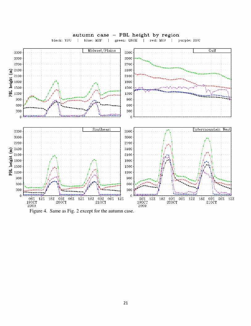
Time series of area-averaged PBL height by region for each case, are shown in Figs. 2-5.

One feature is immediately obvious from these time series: the diurnal cycle in every region

except the Gulf region. Given the high specific heat capacity of water which constitutes the

entirety of the land use type in this region, the lack of a diurnal cycle does make sense. The time

series are the shapeliest for the summer case, perhaps due to the very inactive synoptic scale

conditions during that particular case, but perhaps due to other factors as well. Also apparent

from evaluation of Figs. 2-5 is the ranking of PBL heights for the different PBL schemes. No

matter the season (or region) there is a consistent trend for the QNSE and MYJ schemes to have

the highest PBL heights in that order and for the YSU and MRF schemes to have similar heights

during the daytime and the YSU scheme to have higher heights during the nighttime. Given the

methods by which the QNSE and MYJ schemes compute PBL heights, this ranking makes sense

for these two schemes. Also, since the YSU and MRF schemes compute PBL height in almost

identical ways, and since the simulations with those PBL schemes used the same surface layer

schemes, it makes sense that heights for these two schemes are so close. It should be noted that

similar plots were produced in which the computation of area-averaged PBL height was

computed using grid points for which there was no snow cover and no rain falling at the analysis

time. These plots are not shown because they showed the exact same features and the only

difference between these plots and those which are shown is a simple translation or scaling of

PBL heights towards higher values (falling rain and snow cover thus result in lower PBL heights

overall at a given grid point).

Regarding accuracy, it is apparent from Figs. 2-5 that the YSU and MRF schemes are the

most accurate overall. The MRF scheme is especially accurate during the overnight hours. A

couple of exceptions to this trend are in the summer case in the Gulf region, where the time

10

series for PBL height from the RUC analyses lies between those for the MYJ and QNSE

schemes, and also in the Gulf region late in the autumn case, where again the MYJ scheme

becomes more accurate than either the YSU or MRF scheme. Also it is apparent that the MYJ

and QNSE schemes PBL heights predict too high with the QNSE scheme predicting PBL heights

markedly too high compared to the RUC analyses. Because of the different definition of PBL

height used by the RUC model, the apparent accuracy comes into question. Unfortunately, none

of the PBL schemes in this study use a similar method as the RUC for computing PBL height, so

one is left to wonder how accurate these schemes would be if they used a different method to

compute PBL height.

Although Figs. 2-5 present all of the relevant information obtained from the simulations,

it helps to view the data in different ways as doing so may elucidate additional information. One

example is shown in Fig. 6. The simple change in organization elucidates another obvious

feature: the phasing of the diurnal cycle due to longitudinal position of the various analysis

regions. This is best shown using the summer case. PBL heights in the Southeast region

progress through the diurnal cycle earlier in UTC time than do those in the Midwest & Plains

region, and those in the Midwest & Plains region progress earlier than those in the Intermountain

West region (the lack of a diurnal cycle in PBL heights for the Gulf region makes such an

observation for that region impossible). Plots like Fig. 6 (for the other cases – not shown) also

allow a comparison of how PBL heights vary by region for a given case. Although such a

comparison could also be made by analyzing Figs. 2-5, the comparison is more direct in Fig. 6.

It can be concluded that for every case except for the winter case, PBL heights during the

daytime are highest in the Intermountain West region, whereas those in the Midwest & Plains are

comparable to those in the Southeast region. For the winter case, the Southeast region has the

11

highest PBL heights for the land-dominated regions, probably due to the lack of snowfall and

cold air outbreaks that impact the Midwest & Plains and Intermountain West regions (which

have comparable PBL heights for the winter case). However, PBL heights are highest for the

Gulf region for the winter case. This is due to the high heat capacity of water which comprises

the entire Gulf region and will be further discussed later. Fig. 6 also gives another way of

evaluating the skill of each PBL scheme. The closeness of the solid and dashed time series for

the YSU and MRF schemes again shows that those schemes were more accurate in general.

Another reorganization of the time series are shown in Figs. 7 and 8 which show how

PBL heights vary with season for the Gulf and Intermountain West regions. The high heat

capacity of the Gulf region’s water appears as a time-lagged correlation between season and PBL

height when compared to PBL heights for the Intermountain West region. Thus, PBL heights are

highest in the autumn and winter cases in the Gulf region when all of the intense insolation

incident upon the water surface during the spring and summer seasons finally affects the water

temperature, and they are lowest in the spring and summer by the same logic. Since the specific

heat capacity of soil/land is much lower, there is no apparent time lag in the seasonal trend of

PBL heights for the Intermountain West region. PBL heights are highest during the summer

when the atmosphere in general is warmest and lowest during the winter when the atmosphere is

coldest. The same general pattern holds for the Midwest & Plains and Southeast regions (not

shown), except for a trend for PBL heights to be almost as large in the spring as in the summer

for these regions, a trend not present in the Intermountain West region.

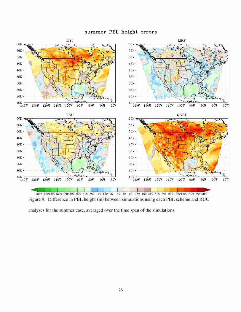
In Figs. 2-8 PBL heights in a region were represented by a single mean value. Spatial

distributions of PBL height differences between the different PBL schemes and the hourly RUC

analyses for each case are shown in Figs. 9-12 with the values of domain averaged differences

12

presented in Table 1. Note that data in these figures and table represent the data averaged over

the entire time spanned by each simulation (i.e., each is an average of 61 hourly plots). These

figures again support the conclusions conjectured earlier in this section that the MRF and YSU

schemes predict PBL height better than the MYJ and QNSE schemes according to the RUC

analyses. However, in every case except the winter case (Fig. 10), both the YSU and MRF

scheme simulations had higher PBL heights than those in the RUC analyses over land (positive

error) and lower PBL heights over water (negative error). Also as has been hinted at already, the

MYJ and QNSE schemes in general predict PBL heights that are too high across most of the

model domain, particularly over much of the CONUS, with the only exceptions being in the

eastern Pacific Ocean, portions of western Canada, and portions of the western Atlantic Ocean

and Caribbean Sea. Figs. 9-12 also show some seasonal biases for the PBL schemes. In

particular in the Gulf of Mexico all four schemes predict too low of PBL heights in the summer

case (with the QNSE scheme as a slight exception) and too high of PBL heights in the winter

case. In each case except for the winter case, every PBL scheme except for the MRF scheme

predicts too high of PBL heights across the Midwest and high plains regions of the CONUS with

the MRF PBL scheme being more accurate in these areas during these cases. None of the PBL

schemes has any significant large-scale bias other than those mentioned, however.

5. Summary, discussion, and conclusions

This study investigated how different PBL parameterization schemes in a NWP model –

the WRF-ARW – predict PBL height over a large portion of North America, which included the

CONUS and surrounding areas. Four PBL schemes in the WRF-ARW that output PBL height

were used in four different real data cases, one from each of the four meteorological seasons, and

13

compared to hourly RUC analyzed PBL heights over four specific regions to compare how well

each PBL scheme predicts PBL height.

The results show that the MRF and YSU schemes appear to be better predictors of PBL

height, although caution must be applied to the results, as the RUC analyses used a definition of

PBL height different from that used by any of the PBL schemes, so differences in PBL height

between the RUC analyses and the various PBL schemes may be a result of factors other than

how well each predicted the actual structure of the boundary layer. On the other hand, the RUC

analyses could be thought of as a “third opinion” as to what the actual PBL height is.

Regardless, these results are somewhat at odds with those of Deng and Stauffer (2006) and Pleim

(2007b) both of which noted that the MRF scheme can predict too high a PBL height. Pleim

(2007b) also noted that the MRF scheme can over mix, resulting in too deep, warm, and dry of a

PBL. Time-height sections of the difference in area-averaged profiles of relative humidity (RH)

in the Midwest and Plains region in the summer case between the PBL schemes and the RUC

analysis data in Fig. 13 clearly show that the lowest 100 hPa or so after about 1800 UTC 14 July

2010 for both the MRF and YSU schemes is drier than in the RUC analyses. Thus, while Fig. 13

shows agreement with the results from Pleim (2007b), the time series in Figs. 2-8 show that the

MRF scheme predicted anything but too high of PBL heights. It should also be noted from Fig.

13 that in the MYJ and QNSE schemes the lowest 100 hPa or so is wetter than in the RUC

analyses. This observation matches the conclusion from G. Thompson (2010, personal

communication) that the YSU scheme produces a dry and warm PBL and the MYJ scheme

produces a cool and wet PBL. However, Fig. 14 shows that this pattern does not hold for every

region, as the PBL in the MYJ and QNSE schemes is drier compared to the RUC analyses and

the MRF and YSU schemes in the summer case. Vogelezang and Holtslag (1996) noted that the

14

use of Ri to compute PBL heights is generally good over land, but may result in high PBL

heights over water in high winds. The simulations in this study show loose agreement with this

generalization for the winter and spring cases, as surface wind speed was moderately positively

correlated with PBL height over water for the YSU and MRF schemes in those cases, but there

was little positive correlation between these variables in the summer and autumn cases. It is

currently unknown why the results of this study differ from those of past studies. Perhaps the

dynamics of the WRF-ARW (unique to this study) are the primary cause. Perhaps the

generalizations made in this and/or the related studies are too general. Perhaps model resolution

plays a role.

The conclusions that can be made from this study include that the MRF and YSU PBL

schemes were better predictors of PBL height overall. Since the depth of mixing and diffusion in

a PBL parameterization scheme depends on the depth of the PBL, this should indicate better

forecasts overall for WRF-ARW simulations that use these two PBL schemes. It is interesting

that the MRF scheme performed so well as it is currently being phased out of newer versions of

WRF-ARW. However, the YSU scheme is essentially an updated version of the MRF PBL

scheme, so the model package is not losing a good PBL scheme without being replaced with

another scheme of equal skill.

Work in this topic could be furthered by rerunning the simulations using higher

horizontal and vertical grid spacing. The simulations could also be run for longer, encompassing

three, four, or more diurnal cycles. The model domain could be expanded to include more of the

world. Different analysis regions could be used. Computer resources limited such work for this

study. Also, it could be worth investigating the range of PBL heights that could be obtained by

using the various methods of computing PBL height that were mentioned in the introduction.

15

The author is unaware of such a study having been undertaken. Finally, as new PBL schemes

are developed, they should also be tested to update the repertoire of more-skilled vs. less-skilled

PBL parameterization schemes.

16

REFERENCES

Busch, N. E., S. W. Chang, and R. A. Anthes, 1976: A multi-level model of the planetary

boundary layer suitable for use with mesoscale dynamic models. J. Applied. Meteor., 15,

909–919.

Cheng, Y., V. M. Canuto, and A. M. Howard, 2002: An improved model for the turbulent PBL.

J. Atmos. Sci., 59, 1550–1565.

Deardorff, J. W., 1972: Parameterization of the planetary boundary layer for use in general

circulation models. Mon. Wea. Rev., 100, 93–106.

----, 1974: Three-dimensional numerical study of the height and mean structure of a heated

planetary boundary layer. Bound.-Layer Meteor., 7, 81-106, doi:10.1007/BF00224974.

Deng, A., and D. R. Stauffer, 2006: On improving 4-km mesoscale model simulations. J.

Applied Meteor. Climatology, 45, 361–381.

Hong, S.-Y., Y. Noh, and J. Dudhia, 2006: A new vertical diffusion package with an explicit

treatment of entrainment processes. Mon. Wea. Rev., 134, 2318–2341.

Melfi, S. H., J. D. Spinhirne, S.-H. Chou, and S. P. Palm, 1985: Lidar observations of vertically

organized convection in the planetary boundary layer over the ocean. J. Climate App.

Meteor., 24, 806–821.

Mellor, G. L., and T. Yamada, 1982: Development of a turbulence closure model for geophysical

fluid problems. Rev. Geophys. Space Phys., 20, 851–875.

Pleim, J., 2007b: A combined local and non-local closure model for the atmospheric boundary

layer. Part II: Application and evaluation in a mesoscale meteorological model. J.

Applied Meteor. Climatology, 46, 1396–1409.

17

Santanello Jr., J. A., M. A. Friedl, and W. P. Kustas, 2005: An empirical investigation of

convective planetary boundary layer evolution and its relationship with the land surface.

J. Applied Meteor., 44, 917–932.

Skamarock, W. C., and Coauthors, 2008: A description of the advanced research WRF version 3.

NCAR/TN–475+STR, 113 pp.

Stull, R. B., 1988: An Introduction to Boundary Layer Meteorology. Kluwer Academic, 666 pp.

Vogelezang, D. H. P., and A. A. M. Holtslag, 1996: Evaluation and model impacts of alternative

boundary-layer height formulations. Bound.-Layer Meteor., 81, 245-269,

doi:10.1007/BF02430331

18

Figure 1. Model and analysis domains.

19

Figure 2. Time series of area-averaged PBL height by region for the summer case.

20

Figure 3. Same as Fig. 2 except for the winter case.

21

Figure 4. Same as Fig. 2 except for the autumn case.

22

Figure 5. Same as Fig. 2 except for the spring case.

23

Figure 6. Time series of PBL heights for the summer case organized by constant PBL scheme in

each panel with each color representing a different analysis region. The solid curves mark

simulation data, while the dashed curves represent RUC analysis data.

24

Figure 7. Time series of PBL heights for the Gulf region organized by constant PBL scheme

within each panel with each color representing a different season. Solid curves denote

simulations while dashed curves denote RUC analysis data.

25

Figure 8. Same as Fig. 7 except for the Intermountain West region.

26

Figure 9. Difference in PBL height (m) between simulations using each PBL scheme and RUC

analyses for the summer case, averaged over the time span of the simulations.

27

Figure 10. Same as Fig. 9 except for the winter case.

28

Figure 11. Same as Fig. 9 except for the autumn case.

29

Figure 12. Same as Fig. 9 except for the spring case.

30

Figure 13. Time-height section of difference in area-averaged relative humidity (%) between

simulations using each PBL scheme and RUC analysis data for the Midwest and Plains region

and summer case. Positive values indicate that the simulation has a higher RH than the RUC

analysis.

31

Figure 14. Same as Fig. 13 except for the Gulf region.

32

Case →

Summer Winter Autumn Spring

PBL scheme

YSU 51.3 81.2 37.9 80.0

MYJ 366.4 457.7 416.0 509.5

QNSE 671.8 706.0 719.0 836.1

MRF -81.6 -27.1 -95.0 -88.4

Table 1. Model-domain averaged PBL height differences (m) from RUC analyses for the

indicated cases and PBL schemes