A MODEL OF TECHNOLOGICAL PROGRESS IN THE MICROPROCESSOR …€¦ · · 2014-07-25that occurred in...

A MODEL OF TECHNOLOGICAL PROGRESS IN THEMICROPROCESSOR INDUSTRY*

UNNI PILLAI†

This paper develops a model of technological progress in the micro-processor industry that connects the seemingly disparate engineeringand economic measures of technological progress. Technological pro-gress in the microprocessor industry is driven by the repeated adoptionof higher quality vintages of capital equipment produced by theupstream semiconductor equipment industry. The model characterizesthe optimal adoption decision of a microprocessor firm and the result-ing rate of technological progress. In conjunction with parametersestimated using a new dataset of the microprocessor industry, themodel suggests explanations for the acceleration in technologicalprogress during 1990–2000 and the subsequent slowdown.

I. INTRODUCTION

A NUMBER OF STUDIES SEEKING TO EXPLAIN THE INCREASE in productivitygrowth in the U.S. economy during the second half of 1990’s credit acentral role to an acceleration in technological progress in the micropro-cessor industry.1 The cause of the acceleration has been debated in manyacademic, industrial and policy forums.2 The rate of technological progress

* I am indebted to Samuel Kortum for his constant encouragement and advice, and forhaving helped me with numerous corrections and revisions to this paper. I am grateful to AnaAizcorbe for her guidance and for sharing her understanding of the semiconductor industrywith me. I thank Evsen Turkay for her valuable help and suggestions. I thank FernandoAlvarez, David Autor, Patrick Bajari, Karna Basu, Thomas Chaney, Rajesh Chandy,Jeremy Fox, Luis Garicano, Thomas Holmes, Ali Hortacsu, Timothy Kehoe, NarayanaKocherlakota, Steven Levitt, Erzo Luttmer, Dan Sichel, Nancy Stokey, John Sutton, ChadSyverson, Harald Uhlig, participants of Applied Microeconomics Workshop at The Univer-sity of Minnesota, Three anonymous referees and the Editor for their suggestions. I thankMark Horowitz and François Labonte for providing the engineering data on microproces-sors. I thank BLS for financial support of the research ‘Equipment Costs in MicroprocessorProduction’ and BEA for providing access to some of the proprietary data used in thisresearch under an IPA agreement. Any errors in the paper are my own.

†College of Nanoscale Science and Engineering, University at Albany, State University ofNew York, 257 Fuller Road, Albany, New York 12203, U.S.A.e-mail: [email protected].

1 Jorgenson [2001] was the first to point out the importance of the microprocessor industry.See also Oliner and Sichel [2002a] and Gordon [2002].

2 See for example the proceedings of the workshop on Measuring and Sustaining the NewEconomy (2002), organized by the Board on Science, Technology and Economic Policy.

THE JOURNAL OF INDUSTRIAL ECONOMICS 0022-1821Volume LXI December 2013 No. 4

© 2013 The Editorial Board of The Journal of Industrial Economics and John Wiley & Sons Ltd

877

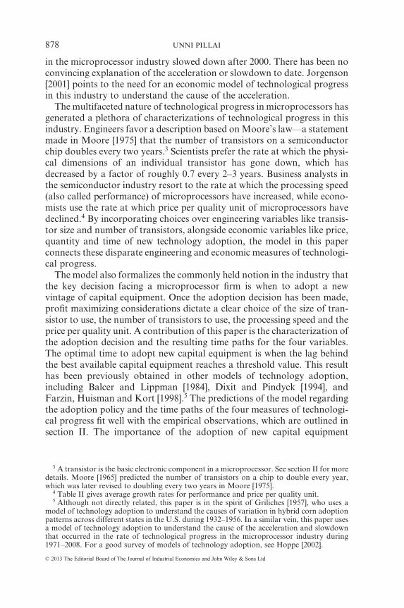
in the microprocessor industry slowed down after 2000. There has been noconvincing explanation of the acceleration or slowdown to date. Jorgenson[2001] points to the need for an economic model of technological progressin this industry to understand the cause of the acceleration.

The multifaceted nature of technological progress in microprocessors hasgenerated a plethora of characterizations of technological progress in thisindustry. Engineers favor a description based on Moore’s law—a statementmade in Moore [1975] that the number of transistors on a semiconductorchip doubles every two years.3 Scientists prefer the rate at which the physi-cal dimensions of an individual transistor has gone down, which hasdecreased by a factor of roughly 0.7 every 2–3 years. Business analysts inthe semiconductor industry resort to the rate at which the processing speed(also called performance) of microprocessors have increased, while econo-mists use the rate at which price per quality unit of microprocessors havedeclined.4 By incorporating choices over engineering variables like transis-tor size and number of transistors, alongside economic variables like price,quantity and time of new technology adoption, the model in this paperconnects these disparate engineering and economic measures of technologi-cal progress.

The model also formalizes the commonly held notion in the industry thatthe key decision facing a microprocessor firm is when to adopt a newvintage of capital equipment. Once the adoption decision has been made,profit maximizing considerations dictate a clear choice of the size of tran-sistor to use, the number of transistors to use, the processing speed and theprice per quality unit. A contribution of this paper is the characterization ofthe adoption decision and the resulting time paths for the four variables.The optimal time to adopt new capital equipment is when the lag behindthe best available capital equipment reaches a threshold value. This resulthas been previously obtained in other models of technology adoption,including Balcer and Lippman [1984], Dixit and Pindyck [1994], andFarzin, Huisman and Kort [1998].5 The predictions of the model regardingthe adoption policy and the time paths of the four measures of technologi-cal progress fit well with the empirical observations, which are outlined insection II. The importance of the adoption of new capital equipment

3 A transistor is the basic electronic component in a microprocessor. See section II for moredetails. Moore [1965] predicted the number of transistors on a chip to double every year,which was later revised to doubling every two years in Moore [1975].

4 Table II gives average growth rates for performance and price per quality unit.5 Although not directly related, this paper is in the spirit of Griliches [1957], who uses a

model of technology adoption to understand the causes of variation in hybrid corn adoptionpatterns across different states in the U.S. during 1932–1956. In a similar vein, this paper usesa model of technology adoption to understand the cause of the acceleration and slowdownthat occurred in the rate of technological progress in the microprocessor industry during1971–2008. For a good survey of models of technology adoption, see Hoppe [2002].

UNNI PILLAI878


highlights the fact that technological progress in microprocessors is drivento a large extent by innovations in the upstream semiconductor equipmentindustry.6 Semiconductor equipment firms like Nikon, Canon, AppliedMaterials and ASML invent new generations of capital equipment whichallows microprocessor firms like Intel and AMD to fabricate smallertransistors, enabling them to make higher performance microprocessors.The notion that the repeated adoption of higher quality vintages of capitalequipment is the driver of technological progress in the microprocessorindustry has been emphasized in Aizcorbe and Kortum [2005].

A distinguishing feature of this paper is that it models technology in theindustry in more detail than is common in economic models. This moredetailed incorporation of the technology turns out to be essential not onlyin connecting the various measures of technological change but also inunderstanding the causes of the acceleration and slowdown in technologi-cal progress in the industry. The detailed modeling of technology helps toseparate out the contribution of the semiconductor equipment firms fromthat of microprocessor firms towards technological progress in the micro-processor industry. There have been many previous studies of the accelera-tion and slowdown, including Jorgenson [2001], Aizcorbe [2005], Aizcorbe,Oliner and Sichel [2008] and Flamm [2004]. The studies above characterizethe rate of technological progress in terms of the rate at which price perquality unit has declined for microprocessors.7 This approach however hasthe limitation, as noted in Aizcorbe, Oliner and Sichel [2008], that changesin prices brought about by changes in demand and competitive conditionscan be mistakenly attributed to changes in the rate of technological pro-gress. To overcome this problem, I use the notion of technological progressas the growth of microprocessor performance.8 Performance, or processingspeed, is a measure of how fast a microprocessor can execute softwareprograms. Nordhaus [2001] gives a detailed description of the use ofperformance as a measure of technological progress in computing, andcompares it with the hedonic price based approach.9 The growth rate ofmicroprocessor performance increased during 1990–2000 and decreasedsubsequently (see Figure 1).10

6 Section II elaborates on this link between technological progress in the microprocessorindustry and the adoption of new vintages of semiconductor equipment.

7 The price per quality unit is estimated using hedonic regressions.8 Performance is the commonly used measure for comparing microprocessors in computer

science. It is the reciprocal of the time that the microprocessor takes to execute a given set ofsoftware programs.

9 Song [2007] and Gordon [2009] are two other papers that use microprocessorperformance.

10 The changes in the growth rate of performance is broadly consistent with the changes inthe growth rate in price per quality unit mentioned in Grimm [1998], Aizcorbe [2006] andAizcorbe, Oliner and Sichel [2008]. See Table II.

A MODEL OF TECHNOLOGICAL PROGRESS 879


The model in this paper implies that in steady state, the mean growth rateof performance is determined by two parameters. The first parameter is therate of innovation in the upstream semiconductor equipment industrywhich determines the rate at which new capital equipment that can fabri-cate smaller transistors becomes available for adoption by microprocessorfirms. The new equipment with smaller transistor size allows microproces-sor firms to use more transistors in their microprocessor. The secondparameter is the efficiency with which the microprocessor firm can convertthe extra transistors to higher performance. This efficiency depends on thequality of microprocessor design (often called microarchitecture), a supe-rior design can get a bigger increase in performance from a given increasein the number of transistors. The model, together with empirical estimatesof the parameters, implies that the acceleration during 1990–2000 wascaused by an increase in the innovation rate in the upstream semiconductorequipment industry, while the slowdown after 2000 was caused by adecrease in the efficiency with which the microprocessor industry used theupstream innovations in capital equipment.

40048008

8085

286

386−DX

486−DX

386−SL

486−SL

Pentium

Pentium ProPentium II

Pentium III

Pentium 4Pentium 4−M

Pentium MPentium EEPentium D

Core Duo

Core 2 ExtremeCore 2 QuadCore 2 DuoCore 2 Solo

8080 8086

8088

80286

80386−DXAm 486

5X86K5

K6K6−2

K6−III

Athlon

Athlon XP

Athlon 64Athlon FXAthlon 64 X2Turion 64 X2Turion 64

Phase−I Phase−II Phase−III.1

11

01

00

10

00

10

00

0

Perf

orm

ance (

m)

1970 1972 1974 1976 1978 1980 1982 1984 1986 1988 1990 1992 1994 1996 1998 2000 2002 2004 2006 2008

Year

INTEL AMD

Figure 1The Acceleration and Slowdown for Intel and AMD

Notes: The data on performance is obtained from two sources, SPEC and BAPCo. Both areindustry consortia which develop benchmarks for measuring performance. Performancenumbers in the graph are normalized by the performance of a standard microprocessor, andhence have no units.

UNNI PILLAI880


These explanations find support in other sources. Jorgenson [2001] sug-gests that the acceleration was caused by a decrease in the technology cyclein the semiconductor industry from three years to two years, a fact con-firmed in Figure 2. An increase in the innovation rate in the semiconductorequipment industry leads to a decrease in the technology cycle, as shown inSection V of this paper. Aizcorbe, Oliner and Sichel [2008] also find supportfor an increase in the innovation rate in the semiconductor equipmentindustry. The decrease in efficiency, which led to the slowdown, occurredbecause after the early 2000’s, microprocessor firms were not able to pursuethe same approach as before to developing new microprocessor designs.During the 1990’s Intel used a particular design approach starting with thePentium and extending it to Pentium II, Pentium III and Pentium IV.However, with Pentium IV, the old design approach lead to an insurmount-able engineering difficulty, the amount of heat created during the operationof microprocessors became too large and rendered the microprocessors

Contact Aligner

Proximity Aligner

Projection Aligner

G−Line StepperG−Line StepperG−Line Stepper

Advanced G−Line StepperAdvanced G−Line Stepper

I−Line Stepper

I−Line 436 nmI−Line 436 nmI−Line 436 nmI−Line 436 nm

I−Line 365 nm

Deep Ultra VioletDeep Ultra Violet

DUV

DUV 248 nmDUV 248 nm

DUV 193 nmDUV 193 nmDUV 193 nmDUV 193 nmDUV 193 nm

Phase Shift MaskPhase Shift MaskPhase Shift MaskPhase Shift MaskPhase Shift MaskPhase Shift MaskPhase Shift MaskPhase Shift Mask

Double Patterning

.04

5.0

65

.09

.13

.18

.25

.35

.5.6

.7.8

11.5

36

10

Vin

tag

e

71 74 76 82 89 91 94 95 98 99 01 04 05 07

Date of Adoption

INTEL AMD

Adoption of Vintages of Semiconductor Equipment

Figure 2Intel and AMD’s Adoption of New Vintages of Semiconductor Capital Equipment

Notes: The date of adoption of a vintage is taken to be the date on which Intel (or AMD)released the first microprocessor manufactured with that vintage. The dates marked on the x-axisare Intel’s adoption dates. Note the decrease in the average time interval between adoptions afterPhase I. This is the reduction in technology cycle that has been noted in Jorgenson [2001],Aizcorbe, Oliner and Sichel [2008] and Flamm [2004].



defective.11 Since the early 2000’s, microprocessor firms have developed anew design approach (the multicore design) which is not as effective inmaking use of transistors as the old design approach. Patterson [2010]provides a lucid account of the transition to the new design approach andthe problems inherent in the new approach.12 This technological explana-tion for the slowdown, acknowledged by the industry experts, has found itsway even to the popular press, with the following quote coming from anarticle in the The New York Times. ‘The computer industry has a secret.Yes, the number of transistors on modern microprocessors continues tomultiply geometrically, but no one really knows how to get the most out ofall these new transistors.’13 To put it simply, the upstream equipment firmsmade available better capital equipment to microprocessor firms at a fasterpace after 1990, but since 2000 the microprocessor firms have been unableto translate the improvements in capital equipment to improvements inperformance at the same rate as before.

The slowdown since 2000 has reduced the contribution of the micropro-cessor industry to aggregate productivity growth. The impact of the accel-eration and slowdown on total factor productivity (TFP) growth in theU.S. economy can be calculated using the method suggested in Oliner andSichel [2002b]. In their method, the aggregate TFP growth is the weightedaverage of the TFP growth in the different sectors in the economy, wherethe weight for each sector is its gross output as a share of the aggregateoutput.14 Using the growth rate of performance as a proxy for the TFPgrowth rate in the microprocessor industry, Table I shows that the contri-

11 Markoff [2011] summarizes the problem: ‘. . . Now, however, researchers fear that thisextraordinary acceleration is about to meet its limits. The problem is not that they cannotsqueeze more transistors onto the chips—they surely can—but instead, like a city that cannotprovide electricity for its entire streetlight system, all those transistors could require too muchpower to run economically. They could overheat, too . . .’ ‘I dont think the chip wouldliterally melt and run off of your circuit board as a liquid, though that would be dramatic,’Doug Burger, an author of the paper and a computer scientist at Microsoft Research, wrotein an e-mail. ‘But you’d start getting incorrect results and eventually components of thecircuitry would fuse, rendering the chip inoperable’. . . . Shekhar Y. Borkar, a fellow at IntelLabs, called Dr. Burger’s analysis right on the dot, . . . Chip designers have been strugglingwith power limits for some time. A decade ago it was widely assumed that it would bestraightforward to increase chips’ clock speed, or the rate at which it makes calculations. Thenthe industry hit a wall at around three gigahertz, when the chips got so hot that they began tomelt. That set off a frantic scramble for new designs.’ The article can be accessed at http://www.nytimes.com/2011/08/01/science/01chips.html?pagewanted=all.

12 The article can be accessed at http://spectrum.ieee.org/computing/software/the-trouble-with-multicore.

13 The quote appeared in an article titled ‘Optimal Use of Transistors Still Elusive,’ by JohnMarkoff, in the September 1, 2009, release of The New York Times. The article can beaccessed at http://query.nytimes.com/gst/fullpage.html?res=9500E5DC1F38F932A3575AC0A96F9C8B63.

14 The theoretical justification for the method is given in Hulten [1978]. Note that thismethod captures only the direct contribution of production of microprocessors to aggregateTFP growth, and omits the indirect effect through the use of better computers made possibleby faster microprocessors.

UNNI PILLAI882


bution of the microprocessor industry to aggregate TFP growth quadru-pled during the acceleration and more than halved during the slowdown.This paper suggests that technological progress in the microprocessorindustry is unlikely to return to the accelerated path during 1990–2000,unless the industry finds a way to increase the efficiency with which it isusing the innovations generated by the upstream semiconductor equipmentindustry. I now turn to a brief description of the connection betweentechnological progress in the microprocessor industry and innovations inthe upstream semiconductor equipment industry.

II. TECHNOLOGICAL PROGRESS IN MICROPROCESSORS

A microprocessor can be thought of as a collection of transistors whichoperate in tandem to execute instructions contained in different softwareprograms. The performance of a microprocessor can be increased either byincreasing the speed of operation of each individual transistor or by usingmore transistors so that more software instructions can be executed simul-taneously (in parallel). The speed of operation of each individual transistoris limited by its size (smaller transistors are faster). The size of each tran-sistor is in turn limited by the quality of the capital equipment used inmanufacturing the microprocessor. Innovations in the semiconductorequipment industry lead to capital equipment that can make smaller tran-sistors.15 The evolution of the microprocessor industry towards faster

15 The equipment industry has a separate classification under the North American Indus-trial Classification System (NAICS Code 333295). Some of the important firms in thisindustry are Applied Materials, Tokyo Electron, Nikon, Canon, ASML, Terdayne andAdvantest. VLSI Research, a market research organization focusing on the semiconductorindustry, estimates the total revenue for the equipment industry in 2007 to be 57.5 billiondollars, 67% of which was accounted for by the top 15 companies. (See SemiconductorInternational [2008].)

TABLE IIMPACT ON AGGREGATE PRODUCTIVITY GROWTH

Phase

Output Share ofMicroprocessors

(%)

TFP Growth inMicroprocessor

Industry (%)

Contribution ofMicroprocessors to Aggregate

TFP Growth (% points)

1971–1989 0.06 28.4 0.0171990–2000 0.14 50.2 0.0702001–2008 0.13 22.9 0.031

Notes: The output share is obtained by multiplying the output share of semiconductors given in Oliner andSichel [2002b] and Oliner, Sichel and Stiroh [2007] by a factor of 0.2, which is roughly the share of micropro-cessors in semiconductor industry revenue. The growth rate of performance is taken as a proxy for the TFPgrowth in the microprocessor industry. The entry in the fourth column is the product of the entries in thesecond and third columns. The fourth column represents only the direct contribution of the production ofmicroprocessors to aggregate TFP growth; it ignores any indirect effect on aggregate TFP growth through theuse of better computers made possible by faster microprocessors.



microprocessors traces the repeated adoption of higher quality vintages ofcapital equipment produced by the semiconductor equipment firms, eachvintage of capital equipment being marked by the size (or length) of thetransistor that the equipment allows the microprocessor industry to make.Since these transistor sizes are really small, they are usually quoted inmicrons (μ), which is a millionth of a meter.

The leading microprocessor firm, Intel, adopted fourteen such vintagesduring the years 1971–2008, 10μ, 6μ, 3μ, 1.5μ, 1μ, 0.8μ, 0.6μ, 0.35μ, 0.25μ,0.18μ, 0.13μ, 0.09μ, 0.065μ and 0.045μ. Figure 2 plots the different vintagesof semiconductor capital equipment that Intel and AMD have adoptedagainst the date of adoption. In the progression through these fourteenvintages from 1971 to 2008, the transistor size has decreased by a factor of222. I use the letter ℓ to denote the vintage of capital equipment which canproduce transistors of size ℓ. A lower ℓ thus implies a higher qualityvintage. I document below four stylized facts about the evolution of thefour measures of technological progress in the microprocessor industrymentioned in the introduction. I denote the time period 1971–1989 as Phase

Phase−I Phase−II Phase−III

0.1

.2.3

.4.5

.6.7

.8.9

1S

calin

g F

acto

r

10 6 3 1.5 1 .8 .6 .35 .25 .18 .13 .09 .065 .045Vintage (l)

Scaling Factor of Transistor Size at each Vintage Adoption

Figure 3The Scaling Factor Does Not Show any Systematic Variation with ℓ

UNNI PILLAI884


I, the period 1990–2000 as Phase II and the period 2001–2008 as PhaseIII.16 The four stylized facts are:

1. The adoption of each new vintage of capital equipment decreases thetransistor size ℓ by roughly the same factor (see Figure 3). For brevity,I will call this the scaling factor.17

2. The number of transistors in a microprocessor, T, increases at roughlydouble the rate at which transistor size ℓ decreases (see Figure 4).

3. Performance, as measured by processing speed, grows at a roughlyconstant rate within each phase. The average growth rate of perfor-mance almost doubled going while from Phase I to Phase II (the accel-eration) and more than halved while going from Phase II to Phase III(the slowdown). (See Figure 1 and Table II.)

4. Price/Performance (price per quality unit) declines at a roughly constantrate within each phase. The average decline rate of price/performance

16 This section, and the other empirical sections of this paper, uses a new dataset of themicroprocessor industry that has been created using data from a variety of sources. SeeAppendix for a description of the data sources.

17 The scaling factor measures the size of the technological improvement that the newcapital equipment provides at each adoption.

Phase−I Phase−II Phase−III

.11

10

10

01

00

01

00

00

Tra

nsis

tors

(m

illio

ns)

10 6 3 1.5 1 .8 .6 .35 .25 .18 .13 .09 .065 .045Vintage (l)

Transistor Evolution with Vintage (slope=2.34)

Figure 4Transistors T Increase at Roughly Double the Rate at which ℓ Decreases. Note that x-axis

Values Are Decreasing to the Right



increased while going from Phase I to Phase II (the acceleration) anddecreased while going from Phase II to Phase III (the slowdown). (SeeTable II.)

Having motivated the role of innovation in the upstream equipment indus-try, the next section develops a model of how the upstream innovationspercolate down and result in technological progress in the microprocessorindustry that is consistent with the stylized facts above.

III. THE MODEL

The model is in continuous time. I develop the model in a few stagesstarting with the semiconductor equipment industry.

III(i). The Semiconductor Equipment Industry

Although the semiconductor equipment industry consists of a large numberof firms which manufacture different types machinery, from the point ofview of technological progress in the microprocessor industry the mostimportant function that these companies serve is that they undertake theR&D necessary to manufacture the next vintage of capital equipment.Hence I lump all these companies together as the semiconductor equipmentindustry. I denote the frontier or highest quality vintage (i.e., the vintagewith the smallest transistor size) by � . The R&D done by the semiconduc-tor equipment industry generates innovations that follow a Poisson processwith parameter λ. Each innovation reduces � by a fixed factor δ, whereδ < 1. Hence the stochastic process for � can be written as

TABLE IIRATE OF TECHNOLOGICAL PROGRESS IN THE MICROPROCESSOR INDUSTRY

Company

Annual Performance Growth Rate (%)

1971–1989 1990–2000 2001–2008

Intel 28.4 50.2 22.9AMD 10.9 65.4 18.5

Source: Author

Annual Hedonic Price Index Decline Rate (%)

1986–1989 1990–1999 2001–2004

Microprocessor Industry 21 47 40.5

Source: Aizcorbe, Oliner and Sichel [2008], Aizcorbe [2006], Grimm [1998]Notes: The top panel shows the average growth rate of microprocessor performance during the three phases.The bottom panel shows the rate of decline of price per quality unit, taken from Grimm [1998], Aizcorbe [2006]and Aizcorbe, Oliner and Sichel [2008]. As can be seen from the table, the growth of performance is broadlyconsistent with the declines in price per quality unit reported in previous studies. In the last phase, thedifference likely arises from the difference in time periods.

UNNI PILLAI886


� �t N t( ) = ( )( )δ 0 ,

N t is a Poisson process with rate( ) λ.

I now turn to a description of the demand side of the model.

III(ii). Demand in the Microprocessor Industry

Consumers care only about the performance of microprocessors. I assumea stationary inverse demand curve, given by,

(1)p tm t

D m t y t( )( )

= ( ) ( )( )−1η ,

where D is a parameter representing market size, p(t) is the price of micro-processor sold at time t, m(t) is the performance (quality) of the micropro-cessor and y(t) is the number of microprocessors demanded. The price perquality unit is p t

m t( )( ) , and m(t)y(t) is the total number of quality units

demanded. The basic assumption behind the demand structure is that totalquality units demanded has a constant elasticity, η, in price per quality unit.One obvious abstraction in this demand specification is the absence ofdynamic decision making by forward looking consumers.18 It is unlikelythat a change in dynamic decision making process by consumers could havebeen a cause of the acceleration and slowdown, so I ignore this aspect ofdemand. I now describe the technology side of the model.

III(iii). Technology in the Microprocessor Industry

A microprocessor firm like Intel chooses the quality (performance) of itsproduct to maximize profits. The common way to model the quality choiceof a firm is to have the firm pay a fixed cost to obtain an improvementin quality (e.g., in Sutton [2001]. The production process in the micro-processor industry, however, gives rise to a peculiar tradeoff betweenperformance and costs not captured in such models. Equations (2) and (3)below, which capture the central aspects of production technology in themicroprocessor industry, illustrate this tradeoff. A firm in the micropro-cessor industry has two ways to increase the performance of its micropro-cessor. First, it can adopt a new vintage of capital equipment which enables

18 See Goettler and Gordon [2011] for a model of the microprocessor industry with forwardlooking consumers.



it to fabricate smaller (lower ℓ) and hence faster transistors.19 Second, it canincrease the number of transistors that it uses in its microprocessor, whichallows the firm to fabricate more units working in parallel in the micropro-cessor, thus increasing performance.20 Performance can thus be written asa function of the number of transistors T and the vintage of capital equip-ment ℓ,

(2) m T mT

, ,��

( ) = 0

α

where m0 is a constant. A microprocessor firm has the choice of increasingperformance by increasing the number of transistors, without having toreduce ℓ by adopting a new vintage of capital equipment. Such anapproach, however, increases the marginal cost of producing a micropro-cessor because it increases the fraction of microprocessors that are defectivein any lot, a feature stemming from the peculiarities of the semiconductorproduction process. In any given lot of microprocessors manufactured, acertain fraction would be defective because of manufacturing imperfectionsarising from contamination by dust particles in the course of production.The fraction of defective microprocessors increases with the physical areaA of the microprocessor because larger microprocessors have a higherprobability of being contaminated by dust particles. A commonly usedyield model in the industry gives the fraction of good microprocessors inany given lot as e−A, where A is the area of the microprocessor.21 Hence, if

19 Reducing ℓ by a given factor increases the speed of each transistor by the same factor (seeRonen et al. [2000] or Borkar [1999]) and hence increases the performance m of the micro-processor by the same factor. ‘Every new process generation brings significant improvementsin all relevant vectors. Ideally, process technology scales by a factor of 0.7 all physicaldimensions of devices (transistors) and wires (interconnects). . . . With such scaling, typicalimprovement figures are the following: 1.4–1.5 times faster transistors; two times smallertransistors . . . ,’ Ronen et al [2000]. The names ‘process generation’ and ‘process technology’in the above quote are terms used in the semiconductor industry to refer to vintages of capitalequipment.

20 The relationship between number of transistors and performance has come to be knownin the semiconductor industry as Pollack’s rule. Fred Pollack was a leading microprocessordesigner at Intel in 1990’s, who observed that a doubling of transistors allowed Intel engineersto build new microprocessor designs that had a roughly 40% increase in performance. Thiswould imply an α of around 0.5. For a good reference on Pollack’s rule, see Borkar and Chien[2011]. Pollack’s rule is a rough rule of thumb and there can be variations in α depending onthe quality of the design used in the microprocessor. In particular, Borkar and Chien [2011]mention that the new designs developed by Intel based on the multicore approach have notbeen able to deliver the same performance increases as predicted by Pollack’s rule.

21 The formula for the fraction good microprocessors (yield) used in this paper, e−A, is calledthe Poisson yield equation. The Poisson yield is usually given as e−aS, where σ is a parameterthat captures the degree of manufacturing imperfections, and S is the physical area of themicroprocessor. For the purposes of this paper, A = σS, can be thought of as the effectivearea, which takes into account the multiplication by σ. See Berglund [1996] for a descriptionof yield models in the semiconductor industry.

UNNI PILLAI888


c is the unit cost of producing a raw microprocessor, the marginal cost ofproducing a good microprocessor is ceA. Since the area of each individualtransistor is ℓ2, the area the microprocessor containing T transistors isA = Tℓ2. Substituting for A, the marginal cost is given by,

(3) c T ceT, � �( ) = 2

Increasing T without reducing ℓ rapidly escalates the marginal cost. Ifthe firm reduces ℓ by adopting a new vintage and increases T in proportionto 1

2�, then the marginal cost remains constant while performance increases.

This is indeed the policy that the model in this paper predicts to be theoptimal policy, as well as the policy that microprocessor firms have fol-lowed in practice (see stylized fact 2 and Figure 4). Although adopting anew vintage allows a microprocessor firm to keep marginal cost constantwhile increasing performance, the firm has to expend a considerableamount of engineering effort in perfecting the production process with thenew vintage of machines.22 I capture this fixed cost with the function F(ℓ),which increases as ℓ decreases. The fixed cost F(ℓ) does not include the usercost of capital, which is incorporated into the unit cost of producing a rawmicroprocessor, c .

The functions m(T, ℓ), c(T, ℓ) and F(ℓ) capture the technology in thisindustry. Note that in the function m(T, ℓ) in equation (2), the ability of amicroprocessor firm to translate increases in T to increases in m depends onthe parameter α. The parameter α is a measure of quality of design used inthe microprocessor. With a superior design (higher α), a microprocessorfirm can get bigger performance increments from a given increase in thenumber of transistors. This design quality is thus a measure of the technicalefficiency of the microprocessor firm. In section V, I argue that a drop inefficiency α caused the slowdown in technological progress in the industry.Using the primitives of demand and technology in sections (III(ii)) and(III(iii)), the next section lays down the profit maximization problem facedby a microprocessor firm.

III(iv). The Profit Maximization Problem of the Microprocessor Firm

Before turning to a formal description of the microprocessor firm’sproblem, I make two assumptions. First, I assume that the market formicroprocessors consists of a single firm facing the demand curve in equa-tion (1). Although there are two major microprocessor producers, Intel and

22 Intel has estimated the cost of adopting the vintage of capital equipment with ℓ = 0.032μto be 7 billions dollars. See Condon [2009].



AMD, Intel has been at the forefront of making innovations in the industrywhile AMD has usually lagged behind. Intel has also occupied 75%–90% ofthe microprocessor market during the time period considered in this paper.Moreover, in a paper exploring whether AMD spurs Intel to innovate,Goettler and Gordon [2011] find that innovation is more an Intel monopolythan an Intel-AMD duopoly. In the light of these arguments, modeling theindustry as a duopoly would complicate the analysis while providing littlehelp in finding explanations for the acceleration and slowdown.23 Second,I assume that the microprocessor firm sells only the highest quality (per-formance) microprocessor. As soon as a better product is made, the entireproduction is moved to the new product. This assumption helps focus onthe factors that determine the rate at which microprocessor performance isgrowing.

Given the Poisson arrival rate λ of innovations to capital equipment,each of which reduces � by a factor δ, the microprocessor firm has tochoose the time paths of performance, marginal cost, the number ofmicroprocessors to produce, the vintage of capital equipment to use, andthe sequence of times at which to adopt new vintages of capital equip-ment, τ j j{ } =

∞0 . The choice of performance and marginal cost can equiva-

lently be stated in terms of choice of the number of transistors and thevintage of capital equipment. Formally, the problem of the microproces-sor firm is,24

max ,, , ,T t t y t

t

j j

E e p t c T y t dt e( ) ( ) ( ) { }

−∞

−

=∞

( ) − ( )[ ] ( ) −∫�

�τ

ρ ρτ

0 0

jj F j

p tm T

D m T y t

j

�

��

τ( )( )⎡

⎣⎢⎢

⎤

⎦⎥⎥

( )( )

= ( ) ( )( )−

=

∞

∑0

subject to,

,11

0

02

η

δ

α

,

, , ,

( ) ( ), ,

m T mT

c T ce

t t

t

T

N t

��

�

� � ��

�( ) = ( ) =

≥ ( )( ) = (

given)) ( ) ( )� 0 , .N t is a Poisson process with rate λ

23 As can be seen in Figure (1), AMD started Phase II as a laggard and caught up with Inteltowards the end of Phase II (see Figure 1). During Phase III, AMD again fell back behindIntel. Hence if competition from AMD does in fact reduce innovation by Intel (as has beenfound in Goettler and Gordon [2011]), then Intel should have had lower growth rate inperformance in Phase II as compared to Phase III. This is the opposite of what is seen in thedata. Hence if Goettler and Gordon [2011] is correct, change in competitive pressure betweenIntel and AMD cannot be the explanation for the acceleration and subsequent slowdown ingrowth rate of Intel’s performance.

24 To avoid notational clutter, I have abbreviated m(T(t), ℓ(t)) as m(T, ℓ) and c(T(t), ℓ(t))as C(T, ℓ) in the statement of the problem.

UNNI PILLAI890


The term in the outer square brackets is the present discounted value ofnet profits, which is the difference between the present discounted valuesof gross profits (the integral term in the objective function) and the sum offixed costs of adopting new vintages (the summation term in the objectivefunction). The first constraint is the demand curve in equation (1), thesecond and third are the technology constraints in equations (2) and (3), thefourth simply states that the firm can at best be using the best vintagecurrently available, and the last specifies the stochastic process for theevolution of the best (frontier) vintage. I restrict η > 1 to make the firm’sproblem well defined.

III(v). Microprocessor Firm’s Optimal Policies

The optimal choice of T and y depend only on the current value of ℓ.Hence I solve the problem by first solving the static problem of choosingT and y for a given ℓ and then embedding this solution back into theproblem, to solve the dynamic problem of choosing the optimal timesτ j j{ } =

∞0 at which to adopt new ℓ. Substituting the constraints into the

objective function, it can be seen that the solution to the static problem isas follows. Along an optimal path of T and y, the following condition hasto hold,

(4) T* ��

( ) = α 12

.

Substituting equation (4) into equation (3) gives marginal cost as

(5) c ce c* *�( ) = ≡α .

The firm’s optimal policy is thus to choose T in proportion to 12�

and hencekeep the marginal cost at c ce* = α , irrespective of the vintage ℓ used. Theoptimality conditions in equations (4) and (5) result from the tradeoffbetween performance and marginal cost explained in section III(iii). Sub-stituting equation (4) into equation (2) gives the optimal performance as,

(6) m mT

m**

��

� �( ) = ( ) = +0 0 1 2

1αα

αα .

i.e., performance grows at 1 + 2α times the rate at which ℓ decreases. Theterm 1 + 2α shows the twin benefits that a microprocessor firm gets fromusing a vintage with a smaller ℓ. The exponent 2α represents the indirectbenefit of smaller ℓ on m through T, and the exponent 1 represents thedirect benefit arising from the fact that smaller transistors are faster. Theoptimal number of microprocessors to produce y*(ℓ) is,



(7) yce

* ��

( ) = −( )η πα ϕ1

1.

where π and φ are given by,

(8) π η αη

α

α

η η

= −( )⎛⎝⎜

⎞⎠⎟

⎛⎝⎜

⎞⎠⎟

−

1 0

1

mce

D,

(9) ϕ α η= +( ) −( )1 2 1 .

Substituting the solutions for m and y into the demand equation (1) givesthe optimal price as,

(10) p ce p* *�( ) =−

⎡⎣ ⎤⎦ ≡η

ηα

1,

i.e., the price of a microprocessor is a constant markup over the marginalcost of production, the term inside square brackets being the marginal costof production. The solutions p* and y*(ℓ) give the revenue along the optimalpath as

(11) r* ��

( ) = η πϕ .

As expected for a constant elasticity demand curve, the gross profit is aconstant fraction 1

η of revenue, and is given by,25

(12) π πϕ* �

�( ) = .

Using the gross profit function in equation (12), the microprocessor firm’sproblem can be rewritten as

max,�

� �t

tj

jj j

jE e t dt e F( ) { }

−∞

−

=

∞

=∞

( )( ) − ( )( )⎡

⎣⎢⎢

⎤∫ ∑

τ

ρ ρτπ τ0 0 0

*⎦⎦⎥⎥

( )( ) =( )

( ) ≥ ( ) ( ) = ( )(

( )

subject to *π π

δ

ϕ��

� � � �

tt

t t t

N t

N t

,

, ,0

)) is a Poisson process with rate λ.

25 Note that π defined in equation (8) is equal to π*(1).

UNNI PILLAI892


I solve the problem using dynamic programming. The dynamic program-ming problem is most conveniently expressed by choosing the state vari-ables as � , the frontier vintage, and x = �

� , which captures how far the firmis behind the frontier. Note that x ≤ 1, since the firm can adopt a vintage nosmaller than � . Since the innovation arrival is Poisson, the probability ofone innovation arriving in a small interval of time Δt is λΔt, and theprobability of more than one innovation is approximately zero. Hence thevalue function should satisfy the Bellman equation,

V x

x

t e t V x

tMax V l x V

t��

�, ,

, ,

( ) =⎛⎝⎜

⎞⎠⎟

+ −( ) ( )⎡⎣

+ ( )

−π λ

λ δ δ δ

ϕρΔ Δ

Δ

Δ 1

�� , .1( ) − ( ){ }⎤⎦F δ

The first term on the right hand side is the profit that the firm receives in asmall interval of time Δt, the second term is the discounted expected payoffafter Δt. With probability 1 − λΔt no innovations arrive in which case thefirm’s value remains at V x�,( ). With probability λΔt one innovationarrives, in which case the firm has to choose between not adopting thisinnovation and getting value V xδ δ�,( ) or adopting it and getting a valueV Fδ δ� �,1( ) − ( ).

I assume that F(ℓ) is homogeneous of degree −φ, the same degree ofhomogeneity as the gross profit function, π*(ℓ). If this were not true, thenone would get a non-stationary model. If F(ℓ) were increasing at a fasterrate in ℓ than π*(ℓ), then the factor by which ℓ scales at each adoption (thescaling factor) would decrease over time, getting closer to 0. If π*(ℓ) wasincreasing at a faster rate than F(ℓ), then the scaling factor would increaseover time, getting closer to 1. However, as Figure 3 shows, the scalingfactor does not show any systematic variation over time, consistent with theassumption that F(ℓ) is homogeneous of degree −φ. The assumption thatF(ℓ) is homogeneous of degree −φ implies that V x�,( ) is homogenous ofdegree −φ in � , and hence V l x l V x v x, ,( ) = ( ) = ( )− −ϕ ϕ1 � , where V(1, x) =v(x). The dynamic program can thus be expressed with a single statevariable, x. Re-writing with the single state variable, and taking the limitΔt → 0, the Bellman equation simplifies to,

(13) ρ π λδ

δϕϕv x x Max v x v F v x( ) = + ( ) ( ) − ( ){ }− ( )⎡

⎣⎢⎤⎦⎥

11 1, .

The left hand side of the equation is the payoff to owning the firm, whichis the sum of the instantaneous payoff and the change in value which occursif an innovation arrives, an event with hazard λ (taking account of the



option to adopt). Proposition 1 characterizes the optimal adoption policyof the firm.

Proposition 1. The optimal policy of the firm is to wait until x falls belowa threshold value x*, where

(14) xv F

* = + −⎛⎝⎜

⎞⎠⎟

( ) − ( )⎛⎝⎜

⎞⎠⎟{ }ρ λ λ

δ πϕϕ1 11

.

See Appendix for proof.Equation 14 can be rearranged to obtain,

(15) ρ π λδ

ϕϕv F x v F v F1 11

1 1 1 1( ) − ( )( ) = + ( )− ( )[ ]− ( ) − ( )[ ]{ }* .

Equation (15) is the value matching condition mentioned in Dixit andPindyck [1994] and Farzin, Huisman and Kort [1998]. The firm adopts atthe point at which the value of adopting is equal to the value of waiting.The value of adopting immediately is the left hand side of the equation, thefirm jumps to the frontier but it has to pay the fixed cost F(1). The term onthe right hand side is the value of waiting which is the sum of instantaneouspayoff and the change in value that occurs if an innovation arrives at thatmoment in time. Note that equation (14) requires ρ λ

δϕ> −( )1 1 .26 Sinceeach innovation shrinks � by δ, this implies that it is optimal to adopt atevery n*th innovation, where n* is the smallest integer such that δ n x* *≤ . Itis easy to summarize the dynamic policy using the simple diagram inFigure 5.

26 If discount factor ρ is not high enough, then discounted net profits are increasing overtime and there will be no solution to the firm’s problem.

Figure 5Adoption Policy of the Firm

UNNI PILLAI894


The possible values of x are 1 2 1, , , ,δ δ δ… n*− . Starting from x = 1, thevalue of x decreases to δ, δ2,.., as the equipment sector produces its streamof innovations. When the n*th innovation arrives, the firm adopts it and xbecomes equal to one again. This cycle repeats.

I summarize the results above. The microprocessor firm adopts everyn*th innovation made by the semiconductor equipment industry and henceℓ used by the firm scales repeatedly by the same factor δ n*. As ℓ decreases,the firm chooses to increase transistor count (T) and performance (m) inproportion to 1

2�and 1

1 2� +( )α respectively. The firm chooses to maintain themarginal cost at c* and charge a price p* per microprocessor, while increas-ing the number of units produced (y) in proportion to 1

�ϕ, where

φ = (1 + 2α)(η − 1). Revenue and gross profits also increase in proportionto 1

�ϕ. This concludes the development of model.

IV. DISCUSSION

In this section I show that the model’s predictions are consistent with thestylized facts documented in section II, and use the model to connectthe four measures of technological progress mentioned in the introduction.The optimal choices of the firm with regard to engineering variables likenumber of transistors and performance, as well as economic variables likequantity, profits and revenue, are determined by the vintage ℓ of capitalequipment that the firm is using, and evolves with the change in ℓ at eachnew vintage adoption. The model thus formalizes the commonly heldnotion in the microprocessor industry that the adoption of new vintages ofcapital equipment is the key driving force in the industry.

The model predicts that at the adoption of each new vintage, the tran-sistor size ℓ should scale by the same factor δ n*, accounting for stylized fact1. As equation (4) shows, the model predicts that the firm’s optimal policyis to increase T in proportion to 1

2�, accounting for stylized fact 2. I show

below that the mean growth rate of m is given by

(16) gm = − +( ) ( )1 2α λ δln .

Thus the mean growth rate of m is constant as long as α and λ does notchange. I argue in section V that changes in gm between the three phaseswere caused by shifts in λ and α. Within each phase, with λ and α fixed, themodel predicts that the mean growth rate of m is constant, accounting forstylized fact 3. Since price p does not change over time, the model predictsthat price/performance ( p

m ) declines inversely with m, accounting forstylized fact 4. The model makes one more testable prediction, that themicroprocessor firm should adopt only occasionally, and should skip someinnovations. In Figure 6, I plot the vintages adopted by Intel (solid hori-zontal lines). The dotted lines are some of the vintages for which capital



equipment was sold by some of the leading semiconductor equipmentproducers, but were not used by Intel.27 As can be seen from the graph,there were quite a number of vintages which Intel did not adopt, in line withthe prediction of the model.28

27 The vintages for the dotted lines were produced by one of the following equipmentcompanies—ASML, Nikon, GCA, SVGL, Parkin-Elmer and Ultratech.

28 Although Intel does not adopt all vintages produced, the equipment firms have anincentive to innovate and produce these vintages because their customers include all compa-nies that make semiconductor chips. In addition to microprocessor producer Intel, companieswho buy semiconductor equipment include producers of memory chips (like Samsung,Micron and Hynix, Toshiba, Fujitsu), producers of semiconductor chips used in electronicdevices (like Sony, Panasonic, Freescale, Fujitsu), as well as contract manufacturers ofsemiconductor chips (like Global Foundries, Taiwan Semiconductor Manufacturing Corpo-ration, etc). These companies probably follow different adoption patterns, influenced by themarket structure and profitability in their own segments. Data collected on semiconductorchips made by other companies (like Samsung) indicate that they have adopted vintages in thepast which were not adopted by Intel.

.04

5.0

65

.09

.13

.18

.25

.35

.6.8

11.5

36

10

Vin

tage (

l)

1970 1973 1976 1979 1982 1985 1988 1991 1994 1997 2000 2003 2006 2009

Year

Vintage Adoptions by INTEL

Figure 6Intel Does Not Adopt all Vintages

Notes: The solid lines are vintages that were adopted by Intel. The dotted lines are vintages thatwere produced by semiconductor equipment firms but were not adopted by Intel. In line with theprediction of the model, Intel does not adopt all vintages produced by semiconductor equipmentfirms. The dotted lines are not the exhaustive list of all vintages, and correspond to only thosevintages for which I could obtain data (from the websites of semiconductor equipmentcompanies or from industry reports).

UNNI PILLAI896


The model connects the four measures of technological progress men-tioned in the introduction. Since the firm’s policy is to adopt every n*thinnovation, the mean growth rate of ℓ will be determined by the stochasticprocess generating the innovations. Proposition (2) gives the mean growthrate of ℓ.

Proposition 2. If the firm adopts every n*th innovation, then the meangrowth rate of ℓ is gℓ = λln(δ).29

See Appendix for proof.

From equation (4) it is clear that T increases at twice the rate at which ℓdecreases, i.e., gT = −2λln(δ). From equation (6) it follows that gm =−(1 + 2α)gℓ. This gives the mean growth rate of m as, gm = −(1 + 2α)λln(δ).Finally, since the price of a microprocessor remains constant over time, theprice per performance decreases at the rate at which performance increases,i.e., gpm = (1 +2α)λln(δ). The four expressions above bring out the relation-ships between the four measures of technological progress in the industry.While the rate of reduction in transistor size (gℓ) and growth in number oftransistors per microprocessor (gT) is fixed by the innovation parameters λand δ in the upstream semiconductor equipment industry, the rate ofgrowth of performance (gm) and price/perperformance (gpm) depend also onthe the efficiency α with which the microprocessor firm uses the upstreaminnovations.

V. EXPLANATIONS FOR THE ACCELERATION AND SLOWDOWN

In this section I use the model to study the acceleration and subsequentslowdown in technological progress, measured as growth of performance. Iwill argue below that the acceleration was caused by an unanticipatedincrease in the upstream innovation rate λ, and the slowdown by an unan-ticipated decrease in the efficiency α with which Intel used upstream inno-vations. These explanations are consistent with the model, since it can beseen from equation (16) that an increase in λ increases gm and a decrease inα decreases gm.30 I explore below whether the model’s predictions about the

29 Note that gℓ < 0 since δ < 1.30 If the changes in α and λ were unanticipated by Intel, the formula derived in the paper

for gm can be used to compare growth across phases. The formula is based on the policies thatIntel would follow, given the values of α and λ. Since these changes were unanticipated, Intelwould select policies assuming the current values of λ and α to continue forever. There isanecdotal evidence to suggest that changes in λ and α were unanticipated. That the change inλ was unanticipated can be seen from ‘The International Technology Roadmap for Semi-conductors,’ a consensus document drawn up every two years by representatives from leadingsemiconductor companies, which projects a timeline for the values of the different parametersin the industry for the next 15 years (see, for example, ITRS [2001]). In versions of theRoadmap in the 1990’s, the forecasts assumed new capital equipment with smaller ℓ to arriveevery three years. The versions of the Roadmap in the early 2000’s noted that new capitalequipment had in fact arrived every two years on average in the 1990s. Gelas [2005] recounts



response of other variables to unanticipated changes in λ and α are con-sistent with the data.

The changes in λ do not affect the static policies—T*(ℓ), m*(ℓ), y*(ℓ), c*

or p*, as can be seen from equations (4)–(10). Such changes do affect thethreshold lag x* in equation (14) and possibly the optimal adoption policy,n*. To characterize the changes in n* induced by changes in λ, I use the factthat any change in n* would affect the present discounted value of the firm.Let V n, λ( ) be the present discounted value of the firm if it adopts every nth

innovation, given an arrival rate λ. Clearly, the optimal adoption policy n*

should satisfy

n V nn

* = ( )arg max , .λ

Proposition 3 derives the function V n, λ( ).Proposition 3. Given the innovation rate λ, the expected present dis-counted value of adopting every nth innovation is

V n

Fn n

, λ

λρ λ

πρ δ

λρ λ

ϕ

ϕ

( ) =−

+⎛⎝⎜

⎞⎠⎟

⎧⎨⎪

⎩⎪

⎫⎬⎪

⎭⎪−

+⎛⎝⎜

⎞⎠⎟

( )

−

11

11

110�

δδλ

ρ λϕ +⎛⎝⎜

⎞⎠⎟

⎡

⎣

⎢⎢⎢⎢⎢

⎤

⎦

⎥⎥⎥⎥⎥

n

See Appendix for proof.

I evaluate the expression V n, λ( ) for plausible parameter values ofδ π ρ ϕ, , , , ,F 1 0( ){ }� for different values of λ and n31. Figure 7 shows the

result of a sample simulation for n = {3, 4, 5}.As can be seen from the figure, n* is weakly increasing with λ, the

intuition for which is provided by the value matching condition in equation(15). An increase in λ increases the value of waiting, the right hand side ofequation (15), since the probability of an innovation’s arriving the nextinstant in time is higher. Hence the firm might find it optimal to wait formore innovations to arrive before adopting. The optimal value n* actuallyincreases only if the increase in λ is sufficiently high. The model thus allows

anecdotal evidence that the change in α was unanticipated by Intel. Intel introduced thePentium chip in 1993 and since then has made extensions of the Pentium design in the formof Pentium II, Pentium III and Pentium 4. But in the early 2000’s, new microprocessorsintroduced with the Pentium 4 design, encountered many engineering difficulties. Intel gaveup on pursuing further extensions of the Pentium 4, and adopted a new design based on amulticore structure. As recounted in the article, Intel had announced plans to push theextensions of the Pentium 4 microprocessors for many years to come, indicating that theproblems that they encountered were unanticipated.

31 The parameter values used are δ = 0.9, F(1) = 1.3, π = 5, ρ = 0.25, φ = 0.86, �0 1= .

UNNI PILLAI898


for the possibility that an increase in λ could occur without inducing anychange in the adoption policy n*. If there were an increase in n* going fromPhase I to Phase II then the scaling factor, δ n*, should have decreased. Theaverage scaling factor has not decreased going from Phase I to Phase II, ascan be seen from Figure 3. The possibility that in going from Phase I toPhase II, there were an increase in λ without a change in n*, finds furthersupport in the data on the time interval between adoptions. Since theadoption interval, Δτj ≡ τj − τj−1, is the time taken for n* Poisson events tohappen, it follows that Δτ λj n∼ G *, 1( ), where G is the gamma distribution.The mean adoption interval is then the mean of G n*, 1

λ( ), which is equal ton*λ . If there were an increase in λ without a change in n*, then the mean

adoption interval, n*λ , should have decreased. The average adoption inter-

val did in fact decrease from 4.35 years in Phase I to 2.10 years in Phase II(this is easily seen in Figure 2).

A change in α affects the static optimal policies. A decrease in α does notchange the elasticity of T*(ℓ) (which still remains at 2) but decreases the

0 0.5 1 1.5 220

25

30

35

40

45

50

55

60

n*=3 n*=4 n*=5

λ

V(n

,λ)

n=3

n=4

n=5

Figure 7Variation of n* with λ

Notes: The y-axis variable, V n, λ( ) is the present discounted value of the firm if it adopts everynth innovation, given arrival rate λ. The optimal adoption policy n* is the value of n thatmaximizes V n, λ( ) . As can be seen from the graph, n* is weakly increasing in λ.



elasticity of the m*(ℓ) which is given by (1 + 2α).32 Indeed, this paper arguesthat a decrease in the elasticity of m*(ℓ) caused the slowdown in growth ofm, and is evident in the data (see Table IV). A decrease in α would alsoreduce the optimal marginal cost c* and price p*. Further, it would reducethe elasticity of the revenue function r*(ℓ) and gross profit function π*(ℓ),both given by φ = (1 + 2α)(η − 1) (see equations (11) and (12)). The lack ofdata on prices, marginal costs and quantity sold for the whole time spanstudied in this paper, makes it difficult to check the predictions of the modelagainst the data for these variables.33 However revenues and gross profitsof Intel are available from Intel’s annual reports.34 Table III reports thevalue of φ estimated using the data from annual reports. The elasticity φdecreased from 0.97 in Phase II to 0.26 in Phase III when estimated fromthe revenue function r*(ℓ), and from 0.99 to 0.28 when estimated from thegross profit function π*(ℓ), consistent with the hypothesis that there was adecrease in α in going from Phase II to Phase III. A change in α would alsochange π (see equation (8)) and hence the threshold lag x* (see equation 14)and possibly the choice of adoption policy n* and the scaling factor δ n*.Similar to the analysis for an unanticipated change in λ above, unless thechange in α is sufficiently large, it will not lead to a change in n*. As can be

32 Note that in referring to elasticity, I take absolute values, for example the elasticity ofm*(ℓ) is ∂ ( )

∂( )m m* *�

��

� .33 According to equation (10), a drop in α from 0.78 to 0.14 (the values estimated for Phase

II and Phase III respectively, as shown in Table IV) should lead to a 47% reduction in prices.The price data for microprocessors for the years 1993–2004 is available from MicroDesignResources. The average price for the period 1993–2000 is 300.36 and the average price during2001–2004 is 228.86. This implies a price drop of 31%, which is less than the 47% predicted bythe model. However, including the price data from years 2005–2008 would probably reducethe price in Phase III to less than 228.86, and reduce the actual drop in price to more than31%. Hence, the drop in α accounts for most of the drop in price seen in the data.

34 During the Phase II and Phase III years, most of Intel’s revenues and profits came fromsales of microprocessors, and hence the revenues and gross profits reported in annual reportscan be taken to be a very close approximation of the revenues and profits from micropro-cessor sales.

TABLE IIIESTIMATES OF φ FROM THE REVENUE FUNCTION AND GROSS PROFIT FUNCTION

Phase II Phase III

Using r*(ℓ) −0.97 −0.26(0.098) (0.12)

Using π*(ℓ) −0.99 −0.28(0.07) (0.19)

Notes: The first row shows φ estimated from the equation ln(r*) = constant + φln(ℓ). The data for revenueswere taken from Intel’s annual reports. The average annual revenue over the years of operation of a vintageℓ is taken as r*(ℓ) . The years of operation of a vintage ℓ is taken to be the years between the year in which ℓwas adopted to the year the next vintage was adopted. The second row shows the estimate for φ obtained witha similar approach using the gross profit function π*(ℓ).

UNNI PILLAI900


seen from Figure 3, the scaling factor δ n* has not changed between PhasesII and III, suggesting again that n* did not change. If neither n* nor λchanged in going from Phase II to Phase III, then the model predicts thatthe mean adoption interval n*

λ should not have changed either. This pre-diction is borne out in the data: the mean adoption interval was 2.03 yearsin Phase II, quite close to the 2.10 years in Phase III. Thus, the changes seenin the data are consistent with what the model predicts should have beenthe response of Intel to an unanticipated increase in λ in Phase I and anunanticipated decrease in α in Phase II.

There are two alternative explanations for the change in the rate oftechnological progress which I examine below. The first candidate is thatthe acceleration in Phase II was caused by a positive demand shock formicroprocessors resulting from the Internet technology boom of the 1990’sand the ensuing slowdown in Phase III was caused by the negative demandshock resulting from the collapse of many technology companies in early2000’s. As shown by equations (8) and (12), a change in D (a positive ornegative demand shock) would lead to a change in profit from any vintage.If the change in profit is sufficiently large, it can in turn affect the adoptionpolicy n* (equation (15)) and hence the frequency of new vintage adoptions.But this would also affect δ n*, the factor by which ℓ scales at each adop-tion. However, as noted in stylized fact (1), the scaling factor has remainedroughly constant across the three phases.35 Further, a positive demandshock can lead to more frequent adoptions with smaller sized technologicalimprovements at each adoption (and a negative demand shock can lead toless frequent adoptions with larger sized technological improvements ateach adoption) but the average growth rate of performance should remainthe same as before (see equation (16)). There was accelerated growth in theindustry for a period of ten years (the duration of Phase II) and slowdownfor over at least eight years, relatively long periods given the pace of growthin the industry. Hence one would like to look for an explanation that allowsfor a change in the average growth rate of performance.

The second candidate explanation for the acceleration and slowdown isthat there were changes in the rate of learning-by-doing in the industry,across the three phases. Learning by doing in the semiconductor industry isprimarily within a vintage and arises from improvements in productionyield over time (see Krugman and Baldwin [1986] and Irwin and Klenow[1994]), as a firm learns to use the new vintage of capital equipment. Whilelearning by doing contributes to the decline in manufacturing cost of agiven microprocessor over its lifetime, it does not play an important role inthe declines in cost per quality unit of microprocessors over long periods of

35 The average values of the scaling factor was 0.6, 0.7 and 0.7 in Phases I, II and IIIrespectively.



time. Such declines result from increases in quality (performance) over timebecause of the adoption of new vintages of capital equipment, with theaverage cost of microprocessors over their lifetimes remaining roughlyconstant. Aizcorbe [2006] finds that average cost per microprocessor com-puted over its lifetime (which corresponds to c in the paper), increasedslightly (by 3.7%) during 1993–1999, and she concludes that reduction incost per microprocessor through learning could not have been a driver ofthe acceleration.

In the next section, I quantitatively assess the contributions of changes inλ and α to the acceleration and slowdown.

V(i). Decomposition of Changes in Growth of Performance

For two time periods t and t′, equation (16) implies that

(17) g

gm

m

t

t

t

t

t

t

′ = ⎛⎝⎜

⎞⎠⎟

++

⎛⎝⎜

⎞⎠⎟

′ ′λλ

αα

1 21 2

.

since δ is assumed to be the same across all periods. A change in the rate oftechnological progress, g

gmt

mt

′ , can thus be neatly separated into contribu-tions from the semiconductor equipment sector, λ

λ′t

t, and from Intel, 1 2

1 2++

′αα

t

t.

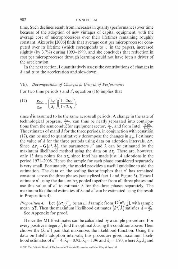
The estimates of α and λ for the three periods, in conjunction with equation(17), can be used to quantitatively decompose the changes in gm. I estimatethe value of λ for the three periods using data on adoption intervals, Δτj.Since Δτ λj n∼ G *, 1( ), the parameters n* and λ can be estimated by themaximum likelihood method using the data on Δτj. There are, however,only 13 data points for Δτj, since Intel has made just 14 adoptions in theperiod 1971–2008. Hence the sample for each phase considered separatelyis very small. Fortunately, the model provides a useful guideline to aid theestimation. The data on the scaling factor implies that n* has remainedconstant across the three phases (see stylized fact 1 and Figure 3). Hence Iestimate n* using the data on Δτj pooled together from all three phases anduse this value of n* to estimate λ for the three phases separately. Themaximum likelihood estimates of λ and n* can be estimated using the resultin Proposition 4).

Proposition 4. Let Δτ j jJ{ } =1 be an i.i.d sample from G n*, 1

λ( ), with samplemean Δτ . Then the maximum likelihood estimates ˆ , ˆn* λ( ) satisfies ˆ ˆλ τ= n*

Δ .See Appendix for proof.

Hence the MLE estimates can be calculated by a simple procedure. Forevery positive integer n*, find the optimal λ using the condition above. Thenchoose the (λ, n*) pair that maximizes the likelihood function. Using thedata on Intel’s adoption intervals, this procedure gives maximum likeli-hood estimates of n* = 4, λ1 = 0.92, λ2 = 1.96 and λ3 = 1.90, where λ1, λ2 and

UNNI PILLAI902


λ3 are the innovation rates in Phase I, Phase II and Phase III respectively.36

The bootstrap distribution of the estimates of n* and λ are given inFigure 9.

For estimating α, equation (6) implies that α can be obtained from theregression, ln(m) = constant + (1 + 2α) ln(ℓ).37 The estimates of λ and α aregiven in Table IV. As can be seen from the table, α dropped in Phase III.

The decomposition of the acceleration and slowdown into contributionsfrom the two sectors, using the estimated values of λ and α, is shown inTable V. Note that a contribution of 1 means that the corresponding sectordid not play a role in the acceleration or slowdown. It can be seen from thefirst row that gm increased by a factor of 1.79 going from Phase I to II . The

36 A larger dataset of all innovations (including those not adopted by Intel) produced by theequipment firms would have allowed the use of other methods to estimate λ independently ofthe estimate of n*. Such a dataset is however not available. While the data on some unadoptedinnovations are available from the website of equipment companies (as shown in Figure 6),this list is not exhaustive. Moreover, the websites and online articles do not usually containthe dates at which equipment was first available in the market.

37 Note that constant in the regression corresponds to ln(m0αα) (see equation (6). Theregression is done separately for each phase and I assume α to be constant in each phase.

Phase−I Phase−II Phase−III.0

1.1

11

01

00

10

00

10

00

0ln

(m)

.045.065.09.13.18.25.35.6.811.53610

ln(l)

Figure 8Strong Relationship between Performance (m) and Vintage (ℓ) in each Phase

Notes: The performance a vintage is taken to be average the performances of allmicroprocessors manufactured with that vintage.



Figure 9Bootstrap Distribution

Notes: For obtaining the distribution for n*, 5,000 random samples (with size of the observedsample) were drawn from a gamma distribution with parameters that were the MLE estimatesobtained from the observed sample. The MLE estimate of n* was calculated for each randomsample to obtain the above distribution. The MLE estimate of n* from the observed sample wasused to calculate the estimate of λ for each phase. For obtaining the distribution of λ’s for eachphase, random samples (with size corresponding to the number of observations in each phase)were drawn from a gamma distribution with the parameters equal to the estimated parameters.The MLE estimate for λ was calculated for each sample, assuming the n* to be the valueestimated from the observed sample. The resulting distribution of λ’s are shown above. Thex-axis values of the vertical dashed lines in the graphs correspond to the estimated parametervalues.

TABLE IVESTIMATES OF α

Phase 1 Phase II Phase III

α 0.53 0.78 0.14(0.18) (0.10) (0.02)

Notes: The parameter α is estimated from the regression ln(m) = constant + (1 + 2α) ln(ℓ). A plot of ln(m)against ln(ℓ) is shown in Figure 8.

UNNI PILLAI904


contribution from semiconductor equipment industry increased by a factorof 2.13 and the contribution from Intel increased by factor of 1.24. Hence,the increase in gm was caused overwhelmingly by an increase in the inno-vation rate in the semiconductor equipment industry λ, and very little wasaccountable to improvements in Intel’s own efficiency α.38 The slowdown,however, was caused entirely by a decrease in Intel’s own efficiency α, ascan be seen from the second row of Table V.

The finding that there was an increase in the innovation rate λ in thesemiconductor equipment industry after Phase I has been corroborated inother studies, including Jorgenson [2001] and Aizcorbe, Oliner and Sichel[2008], who report it in terms of decrease in the time interval between theadoption of new vintages. A possible explanation for the increase in λ,suggested in Hutcheson [2005], is that it was the outcome of R&D coordi-nation activities in the semiconductor equipment industry undertaken bySEMATECH, an industrial research consortium established in 1988.39 It

38 The two contributions taken together account for more than the 1.79 factor increase inperformance seen in the data, and this discrepancy must be taken to be the result of factorsnot taken into consideration in this model. One possible explanation for this is that the firstadopters of semiconductor equipment during Phase I were DRAM (memory chip) producersand not microprocessor producers. In the later years, microprocessor firms adopted at thesame time, if not earlier, than DRAM producers. The presence of possible adoption lagsduring Phase I would mean that the actual innovation rate λ1 is lower than the estimatedvalue, which might account for the discrepancy above.

39 Faced with continuing loss of market share to Japanese companies, in 1988 leading U.S.semiconductor companies formed a research consortium, SEMATECH, with the help of anannual subsidy from the U.S. government. SEMATECH started issuing biennial TechnologyRoadmaps stating the technological barriers to be overcome to create the next vintage ofsemiconductor equipment, and the possible solutions to overcome these barriers. Theroadmaps proved to be a tremendous success in the industry, and turned out to be a point ofcoordination among the different firms in the industry. This success led SEMATECH gave upits national focus and it became International SEMATECH, and the roadmap was renamedthe ‘International Technology Roadmap for Semiconductors’ (ITRS). SEMATECH contin-ues to the be a central point for coordinating R&D in semiconductor equipment, and thebiannual release of the ‘International Technology Roadmap for Semiconductors’ is continu-ing to this day. Flamm [2010] contains an excellent summary of the evolution of

TABLE VDECOMPOSITION OF THE ACCELERATION AND SLOWDOWN

Change in Rate ofTechnological Progress

Contribution ofEquipment. Co.

Contributionof Intel

g

gmtmt

′ λλ′tt

1 21 2++

′αα

tt

Acceleration 1.79 2.13 1.24Slowdown 0.46 0.97 0.50

Notes: Equation (16) stipulates that the entries in the second column should equal the product of the entriesin the third and fourth columns. A value of 1 for the third or fourth column means that the correspondingsector did not play any role in the change in gm. As can be seen from the entries in the second row, theequipment firms played the important role in the acceleration; the role played by Intel was minimal. For theslowdown, on the other hand, Intel was responsible and the equipment companies hardly contributed.



remains a topic of further research to understand the cause of the increasein the innovation rate, and to examine the possible role played bySEMATECH. On the other hand, there is widespread agreement in thesemiconductor industry on the reason for the drop in efficiency α, whichcaused the slowdown. As mentioned in section I, in the early 2000’s, micro-processors with new designs introduced by Intel hit a well publicizedproblem, the microprocessors generated a large amount of heat duringtheir operation which affected their proper functioning. Since then Intel hasabandoned the pattern of design improvements that it had followed in thepast and adopted a new approach, the multicore design. The multicoreapproach is less effective than previous approaches in translating increasesin the number of transistors available on a chip to increases in performance.The inability of Intel’s designs to get the most out of the new transistors iscaptured in the model as a drop in the efficiency α.

Finally, it should be noted that although the explanations for the accel-eration and slowdown suggested here are based on shifts in model param-eters, there are key relationships in the model that have not changed acrossthe three phases. The scaling factor has remained roughly constant acrossthe three phases (see Figure 3). Similarly, the relationship between T and ℓhas not changed across the three phases (see Figure 4).

VI. CONCLUSION

This paper develops an economic model of the microprocessor industrythat endogenizes technological progress in the industry. The model cap-tures well the evolution of different engineering and economic variables inthe industry and connects the engineering and economic measures of tech-nological progress. The model was used to understand the cause of theacceleration in technological progress in the industry during 1990–2000 andthe subsequent slowdown. Three conclusions emerge from this applicationof the model. First, the acceleration in technological progress was driven byan increase in the innovation rate in the upstream semiconductor equip-ment industry leading to more rapid adoption of innovations by Intel.Second, the slowdown was caused by a decrease in the efficiency with whichIntel was able to use the innovations generated by the semiconductorequipment industry. Third, innovation in the semiconductor equipmentindustry has been the main workhorse driving technological progress inthe microprocessor industry since 2001. However, further innovation in thesemiconductor equipment industry is becoming ever more difficult as the

SEMATECH, its role in coordinating R&D efforts across semiconductor companies throughthe road-mapping process, and its impact on innovation in the semiconductor equipmentindustry.

UNNI PILLAI906


industry approaches the physical limit to reducing the size of the transistor.If innovations in the semiconductor equipment industry slow down, then itwill accentuate the existing difficulties in maintaining the rate of techno-logical progress in the microprocessor industry.

APPENDIX

Proofs of Propositions

Proof of Proposition 1. Equation (13) can be rewritten as

v x x Max v x v F( ) =+

++

( ) ( ) − ( ){ }[ ]πρ λ δ

λρ λ

δϕϕ1

1 1,

where x ∈ (0, 1]. Consider the operator T, that maps functions defined on (0, 1] as

T f x x Max f x f F( )( ) =+

++

( ) ( ) − ( ){ }[ ]πρ λ δ

λρ λ

δϕϕ1

1 1,

T(.) maps continuous functions to continuous functions. Moreover, it is easily seenfrom the conditions in Blackwell [1965] that T is a contraction mapping. Hence by thecontraction mapping theorem there exists a unique v(x) that solves the Bellmanequation above. Moreover, T maps weakly increasing functions to strictly increasingfunctions, hence v(x) is strictly increasing (see Stokey, Lucas and Prescott [1989]).Hence, there exists a value x* such that

(18) v x v F*( ) = ( ) − ( )1 1 .

Moreover, since v(.) is an increasing function and δ < 1

(19) v x v Fδ *( ) < ( ) − ( )1 1 .

Evaluating the Bellman equation (VI) at x = x* and using equations (18) and 19 gives,

v x x Max v x v F* * *( ) =+( )

++( )

( ) ( ) − ( ){ }πρ λ δ

λρ λ

δϕϕ1

1 1, [ ]

v F x v F1 11

1 1( ) − ( ) =+( )

++

( ) − ( )[ ]πρ λ δ

λρ λ

ϕϕ*

which gives

xv F

* = + −⎛⎝⎜

⎞⎠⎟

( ) − ( )⎛⎝⎜

⎞⎠⎟{ }ρ λ λ

δ πϕϕ1 11

□



Proof of Proposition 2. Let ℓ0 be the value of ℓ at time t and let ℓ′ be the randomvariable representing the value of ℓ after time interval Δt. The mean growth rate ofℓ is,

(20) gE

tt�

� �= ′( )( ) − ( )

→lim

ln lnΔ Δ0

0

Denote by n the random variable representing the number of innovations thatarrive in time interval Δt, and denote by m the random variable representing thenumber of adoptions that the firm makes in time interval Δt. Since the firm adoptsevery n*th innovation, m is the greatest integer less than n

n* , i.e.,

(21) mnn

= ⎡⎣⎢

⎤⎦⎥*,

Therefore, ′ = ( )� �δ n m*0, and

(22) E E m E mn nln ln ln ln ln .′( )( ) = ( ) + ( )( ) = ( ) ( ) + ( )� � �δ δ* *0 0

From equation (21),

(23) E m Enn

E nn

tn

( ) = ⎡⎣⎢

⎤⎦⎥

⎛⎝⎜

⎞⎠⎟ =

( ) =* * *

λΔ,

where the last step follows from the fact that the expected number of arrivals in timeinterval Δt for a Poisson process with rate parameter λ is λΔt. Substituting equation(23) in equation (22) gives,

E nt

ntln ln ln ln ln .′( )( ) = ( ) + = ( ) +� � �*

*δ λ λ δΔ

Δ0 0

Hence equation (20) implies,

gt

tt�

� �= ( ) + ( ) − ( ) = ( )

→lim

ln ln lnln

Δ

ΔΔ0

0 0λ δ λ δ □

Proof of Proposition 3. Let Δτ j j{ } =∞

0 be the adoption intervals. Then the ith adop-

tion with vintage � �in i

= ( )δ 0 , occurs at time τ τi jj

i

==

−

∑Δ0

1

. Then if the firm follows the

policy of adopting every nth innovation, the net profit of the firm in the ith adoptioninterval (i.e., the profit from operating the ith vintage equipment), discounted back tot = 0 is, Πi(n, λ) =

e e dtF

eii k

kt

ni ni

− −−

( )− ( )( )

⎧⎨⎪

⎩⎪

⎫⎬⎪

⎭⎪=∫ =ρτ ρ

ϕτ

ϕ

ρ τπ

δ δ� �00

0

10

Δ Δii

ini e F

−

∑−( ) − ( )⎧

⎨⎩

⎫⎬⎭

−

1

11 1

0δπρϕ

ρ τ

�Δ

UNNI PILLAI908


Then the present discounted value of net profits obtained under the policy of adopting

every nth innovation is Πii

n, λ( )=

∞

∑0

, which is given by Πii

n, λ( ) ==

∞

∑0

1 1 11

0 0 1

0

1

0

1

�ϕρ τ ρ τ

δ ϕπρ δ ϕn

in

iie

ie F

kk

i

kk

i

−

=

∞ −

=

∞=

−

=

−

∑−

∑( ) −∑ ∑

Δ Δ 110

0 δ ϕπρ

ρ τ

ni i

ek

k

i

−

=

∞=∑ ⎛

⎝⎜⎞⎠⎟

⎡

⎣

⎢⎢

⎤

⎦

⎥⎥∑

Δ

Then V n E n

E e

ii

n ii

kk

i

, ,λ λ

δπρϕ ϕ

ρ τ

( ) = ( )

=∑⎡

⎣

⎢⎢

⎤

⎦

⎥⎥

=

∞

−

=

∑

=

−

Π

Δ

0

0 0

1 10

1

� *

∞∞ −

=

∞

∑ ∑⎡

⎣

⎢⎢

− ( )∑⎡

⎣

⎢⎢

⎤

⎦

⎥⎥

− ⎛⎝⎜

⎞

=

−

11

1

0

1

1 δ

δπρ

ϕ

ρ τ

ϕ

n ii

n i

F E ek

k

i

*

*

Δ

⎠⎠⎟∑⎡

⎣

⎢⎢

⎤

⎦

⎥⎥

⎤

⎦

⎥⎥

−

=

∞=∑ E e

kk

i

i

ρ τΔ0

0

The adoption interval Δτj is the time taken for n* Poisson events to happen. Hence Δτj

are independent draws from the Gamma distribution G n*, 1λ( ). It follows that

∑ ( )=−ji

j n i01 1Δτ λ∼ G * , . To evaluate the above expectations, I use Proposition 5, which

shows that E e in−

+⎡⎣ ⎤⎦ = ( )ρ τ λρ λ

Δ *. This implies

V n E nii

n i

n i

in i

, ,λ λ

δπρ

λρ λ δϕ ϕ ϕ

( ) = ( )

=+

⎛⎝⎜

⎞⎠⎟

−

=

∞

=

∞

∑

∑

Π0

0 0

1 1 1

� *

*

* FFn i

in i

n i

i

11

1

1

0

( )+

⎛⎝⎜

⎞⎠⎟

− ⎛⎝⎜

⎞⎠⎟ +⎛⎝⎜

⎞⎠⎟=

∞ +( )

=∑ λ

ρ λ δπρ

λρ λϕ

*

*

*∞∞

∑⎡

⎣⎢⎢

⎤

⎦⎥⎥

Evaluating the sums of geometric series, the above expression reduces to

V n E nii

n

, ,λ λ

λρ λ

πρ δ

λρ λ

ϕ

ϕ

( ) = ( ) =−

+⎛⎝⎜

⎞⎠⎟

⎧⎨⎪

⎩⎪

⎫⎬⎪

⎭⎪−

+

=

∞

∑Π0 0

11

1

�

⎛⎛⎝⎜

⎞⎠⎟

( )

−+

⎛⎝⎜

⎞⎠⎟

⎡

⎣

⎢⎢⎢⎢⎢

⎤

⎦

⎥⎥⎥⎥⎥

n

n

F 1

11δ

λρ λϕ

□

Lemma 5. If Δτ λi n∼ G *, 1( ), then E e in−

+⎡⎣ ⎤⎦ = ( )ρ τ λρ λ

Δ *

Proof of Lemma 5. Since G nn

jn je

n** *

*, 11

λλ τ λ τ

( ) =− −

( )ΔΓ

Δ

, where Γ(n*) = (n − 1)! is the

Gamma function,



E e ee

nd

nn

i tn n T n

− −− −∞

⎡⎣ ⎤⎦ = =( )

−+∫ρ τ ρ

λλ τ τ λρ λ

τΔ ΔΓ

ΔΓ

Δ* * *

**1

0

1( )*

nn

n n

e d

nn

*

* **

*

− − +( )∞∫

=+

⎛⎝⎜

⎞⎠⎟

−( )( )

=+

⎛⎝⎜

⎞⎠⎟

20

1

ρ λ τ τ

λρ λ

λρ λ

Δ Δ

Γ!

Proof of Proposition 4. Using the p.d.f for gamma distribution, the probability thatthese J observations are drawn from G n*, 1

λ( ) is

λ τ λ τnjn

j

J e

n

j* *

*

ΔΓ

Δ− −

= ( )∏1

1

where Γ(n*) = (n* − 1)! is the gamma function. The log-likelihood function is then

L n n n n

J

j jj

J

* * * *, ln ln ln

ln

λ λ τ λ τ( ) = − ( )[ ] + ( ) + −( ) ( ) −{ }

= −

=∑ Γ Δ Δ

Γ

11

nn Jn n jj

J

jj

J

* * *( )[ ] + ( ) + −( ) ( ) −= =∑ ∑ln lnλ τ λ τ1

1 1

Δ Δ

Let ( ˆ , ˆn* λ ) be the maximum likelihood estimate. Then ∂∂ ( ) =L nλ λˆ , ˆ* 0, which gives

JnjJ

jˆˆ*

λτ− ∑ ==1 0Δ and hence ˆ ˆ ˆλ

τ τ= =∑ =

Jn n

jJ

j

* *

1 Δ Δ .

Data Sources

The dataset contains the following characteristics for every microprocessor made byIntel since the first microprocessor in 1971—product name, date of release, perfor-mance (m), vintage (ℓ), transistors (T). There are a total of 588 microprocessors forIntel. Among these, 135 microprocessors are in the low value category, which Intelsells under the name Celeron. These are usually defective parts which are sold at a lowprice. Hence I omit these microprocessors in this paper. This leaves a total of 453microprocessors for Intel. The server processors manufactured by Intel have also beenleft out since functionally they are very different from desktop and laptop micropro-cessors, which form the focus of this paper. The data for m was obtained from twosources—Standard Performance Evaluation Corporation (SPEC) and BusinessApplications Performance Corporation (BAPCo). SPEC and BAPCO are industryconsortia of which both microprocessor producers, Intel and AMD, are members.The data for T and ℓ were obtained from The Intel website and confirmed againstother online reports and articles.

REFERENCES

Aizcorbe, A., 2005, ‘Moore’s Law, Competition and Intel’s Productivity in the Mid-1990’s,’ American Economic Review, 95, pp. 305–308.

Aizcorbe, A., 2006, ‘Why Did Semiconductor Price Indexes Fall So Fast in the 1990’s?A Decomposition,’ Economic Inquiry, 44, pp. 485–496.

UNNI PILLAI910


Aizcorbe, A. and Kortum, S., 2005, ‘Moore’s Law and the Semiconductor Industry: AVintage Model,’ Scandinavian Journal of Economics, 107, pp. 603–630.

Aizcorbe, A.; Oliner, S. D. and Sichel, D. E., 2008, ‘Shifting Trends in SemiconductorPrices and the Pace of Technological Progress,’ Business Economics, 43, pp. 23–29,Palgrave Macmillan.

Balcer, Y. and Lippman, S. A., 1984, ‘Technological Expectations and Adoption ofImproved Technology,’ Journal of Economic Theory, 34, pp. 292–318.

Baldwin, R. and Krugman, P., 1986, ‘Market Access and International Competition: ASimulation Study of 16K Random Access Memories,’ working paper, NBER.(National Bureau of Econmic Research, Cambridge, Massachusetts, U.S.A.)

Berglund, C. N., 1996, ‘A Unified Yield Model Incorporating Both Defect andParametric Effects,’ IEEE Transactions on Semiconductor Manufacturing, 9, pp. 447–454.

Blackwell, D., 1965, ‘Discounted Dynamic Programming,’ Annals of MathematicalStatistics, 36, pp. 226–235.

Borkar, S., 1999, ‘Design Challenges of Technology Scaling,’ IEEE Micro, 19, pp.23–29.

Borkar, S. and Chien, A., 2011, ‘The Future of Microprocessors,’ Communications of theACM, 54, 67–77.

Condon, S., 2009, ‘Intel to Invest $7 Billion in U.S. Manufacturing Facilities CNET,http://news.cnet.com/8301-13578 3-10160368-38.html.

Dixit, A. K. and Pindyck, R. S., 1994, Investment under Uncertainty (Princeton Univer-sity Press, Pinceton New Jersey, U.S.A.).

Farzin, Y. H.; Huisman, K. J. M. and Kort, P. M., 1998, ‘Optimal Timing of Technol-ogy Adoption,’ Journal of Economic Dynamics and Control, 22, pp. 779–799.

Flamm, K., 2004, ‘Moore’s Law and the Economics of Semiconductor Price Trends,’ inD. W. Jorgenson and C. W. Wessner (eds), Semiconductors: Trends, Implications, andQuestions Report of a Symposium, pp. 151–170. (National Academies Press, 500 FifthStreet N.W., Washington, D.C., U.S.A.).

Flamm, K., 2010, ‘Economic Impacts of International R&D Coordination:SEMATECH and the International Technology Roadmap,’ in Nagaoka S., KondoM., Flamm K. and Wessner C. (eds), 21st century Innovation Systems for Japan andthe United States: Lessons from a Decade of Change, pp. 108–125. (National Acad-emies Press, 500 Fifth Street N.W., Washington, D.C., U.S.A.).

Gelas, J. D., 2005, ‘The Quest for More Processing Power, Part One: Is the Single CoreCPU Doomed?,’ http://www.anandtech.com/show/1611.

Goettler, R. L. and Gordon, B. R., 2011, ‘Does AMD Spur Intel to Innovate More?,’Journal of Political Economy, 119, pp. 1141–1200.

Gordon, B. R., 2009, ‘A Dynamic Model of Consumer Replacement Cycles in the PCProcessor Industry,’ Marketing Science, 28, pp. 846–867.

Gordon, R. J., 2002, ‘Technology and Economic Performance in the AmericanEconomy,’ NBER working paper 8771, (National Bureau of Economic Research).

Griliches, Z., 1957, ‘Hybrid Corn: An Exploration in the Economics of TechnologicalChange,’ Econometrica, 25, pp. 501–522.

Grimm, B., 1998, ‘Price Indexes for Selected Semiconductors, 1974–96,’ Survey ofCurrent Business, pp. 824.

Hoppe, H. C., 2002, ‘The Timing of New Technology Adoption: Theoretical Modelsand Empirical Evidence,’ Manchester School, 70, pp. 56–76.

Hulten, C. R., 1978, ‘Growth Accounting with Intermediate Inputs,’ The Review ofEconomic Studies, 45, pp. 511–518.

Hutcheson, D., 2005, ‘The R&D Crisis,’ discussion paper (VLSI Research, Santa ClaraCalifornia, U.S.A.).



Irwin, D. A. and Klenow, P. J., 1994, ‘Learning-by-Doing Spillovers in the Semicon-ductor Industry,’ Journal of Political Economy, 102, pp. 1200–1227.

ITRS, 2001, The International Technology Roadmap for Semiconductors, technicalreport, (Austin, Texas, U.S.A.) online at ITRS above.

Jorgenson, D. W., 2001, ‘Information Technology and the U.S. Economy,’ AmericanEconomic Review, 91, pp. 132.

Markoff, J., 28 July, 2011, ‘Progress Hits Snag: Tiny Chips Use Outsize Power,’ TheNew York Times.

Moore, G. E., 1965, ‘Cramming More Components onto Integrated Circuits, Electron-ics, 38, pp. 114–117.

Moore, G. E., 1975, ‘Progress in Digital Integrated Electronics,’ IEEE, IEDM TechnicalDigest, pp. 11–13.

Nordhaus, W. D., 2001, ‘The Progress of Computing,’ discussion paper 1324, (CowlesFoundation, Yale University, New Haven, Connecticut, U.S.A.).

Oliner, S. D. and Sichel, D. E., 2002a, ‘Information Technology and Productivity:Where Are We Now and Where Are We Going?,’ Finance and Economics DiscussionSeries 2002-29, (Board of Governors of the Federal Reserve System ConstitutionAvenue, N.W., Washington, D.C., U.S.A.).

Oliner, S. D. and Sichel, D. E., 2002b, ‘The Resurgence of Growth in the 1990’s: IsInformation Technology the Story?,’ Journal of Economic Perspectives, 2000, pp.3–22.

Oliner, S. D.; Sichel, D. E. and Stiroh, K. J., 2007, ‘Explaining a Productive Decade,’Finance and Economics Discussion Series 2007-63, (Board of Governors of the FederalReserve System Constitution Avenue, N.W., Washington, D.C., U.S.A.).

Patterson, D., 2010, ‘The Trouble with Multicore,’ IEEE Spectrum, 47, pp. 28–32.Ronen, R.; Mendelson, A.; Lai, K.; Lu, S. L.; Pollack, F. and Shen, J. P., 2000, ‘Coming

Challenges in Microarchitecture and Architecture,’ Proceedings of the IEEE, 89, pp.325–340.

Semiconductor International, 2008, ‘VLSI Research Ranks Top Equipment Vendorsfor 2007,’ www.semiconductor.net/article/CA6541940.html.

Song, M., 2007, ‘Measuring Consumer Welfare in the CPU Market: An Application ofthe Pure Characteristics Demand Model,’ RAND Journal Of Economics, 38, pp.429–446.

Stokey, N. L.; Lucas, R. E. and Prescott, E., 1989, Recursive Methods in EconomicDynamics (Harvard University Press, Cambridge Massachusetts, U.S.A.).

Sutton, J., 2001, Technology and Market Structure: Theory and History, vol. 1 (The MITPress, Cambridge Massachusetts, U.S.A.).

UNNI PILLAI912


A MODEL OF TECHNOLOGICAL PROGRESS IN THE MICROPROCESSOR …€¦ · · 2014-07-25that occurred in...

Documents

Transcript of A MODEL OF TECHNOLOGICAL PROGRESS IN THE MICROPROCESSOR …€¦ · · 2014-07-25that occurred in...