A Model-Based Receiver for CPM Signals in a … · propose an improved demodulation scheme, ......
89
A Model-Based Receiver for CPM Signals in a Cochannel Interference Limited Environment by Pierre Barthelemy Thesis submitted to the Faculty of the Virginia Polytechnic Institute and State University in partial fulfillment of the requirements for the degree of Master of Science in Electrical Engineering Brian D. Woerner, Chair Amy E. Bell Jeffrey H. Reed May 2002 Blacksburg, Virginia Keywords: Parametric Frequency Estimation, Cochannel Interference, MSK, Equalization Copyright 2002, Pierre Barthelemy
-
Upload
nguyenxuyen -
Category
Documents
-
view
225 -
download
0
Transcript of A Model-Based Receiver for CPM Signals in a … · propose an improved demodulation scheme, ......
A Model-Based Receiver for CPM Signals
in a Cochannel Interference Limited Environment
by
Pierre Barthelemy
Thesis submitted to the Faculty of the Virginia Polytechnic Institute and State University
in partial fulfillment of the requirements for the degree of
Master of Science in
Electrical Engineering
Brian D. Woerner, Chair
Amy E. Bell
Jeffrey H. Reed
May 2002
Blacksburg, Virginia
Keywords: Parametric Frequency Estimation, Cochannel Interference, MSK, Equalization
Copyright 2002, Pierre Barthelemy

© Copyright 2002
by
Pierre Barthelemy
A Model-Based Receiver for CPM Signals
in a Cochannel Interference Limited Environment
by Pierre Barthelemy
Committee Chairman: Brian D. Woerner Electrical Engineering
Abstract
Cochannel interference (CCI) is a major impairment in narrowband cellular
systems. To increase the spectral efficiency of the narrowband systems, identical carrier
frequencies are reused in distant cells. The interference rejection capability of the
receiver determines this frequency reuse and is therefore critical. In this thesis, we
propose an improved demodulation scheme, employing high-resolution frequency
estimation techniques, for continuous phase modulated (CPM) signals in presence of
CCI. Minimum shift keying (MSK), which is a special case of CPM, is a very popular
modulation format around the world. Frequency detectors, such as the limiter-
discriminator permit the non-coherent demodulation of MSK signals. High-resolution
frequency estimation appears as a very attractive alternative to the conventional non-
coherent frequency detectors. The frequency estimation methods that we have studied are
based on autoregressive modeling.
The contributions of this thesis include the implementation of various
demodulation schemes employing parametric frequency estimation. The use of the
Viterbi algorithm as a non- linear equalization technique to mitigate intersymbol
interference is considered. We verified that the model-based sequence estimation
schemes outperform the conventional non-coherent receivers for MSK with AWGN, flat
fading, and CCI. Demodulator diversity is also investigated as a way to combat
interference. An improved technique combining the proposed model-based receiver and
the conventional coherent receiver is implemented and simulated in presence of CCI.

iv
Acknowledgments
Foremost I would like to thank my advisor, Dr. Brian D. Woerner, for his support
and guidance. I am sincerely grateful to him for giving me the opportunity to work at the
Mobile and Portable Radio Research Group (MPRG) among excellent students and with
a very cooperative staff. I wish to express my gratitude to my committee members, Dr.
Amy E. Bell and Dr. Jeffrey H. Reed, for their encouragements and for reviewing this
thesis.
During the course of this thesis, it has been a pleasure to work with Yasir Ahmed
on frequency estimation. I also thank all of my friends from MPRG for their help on
technical and non-technical matters.
This research has been sponsored by the MPRG Industrial Affiliates program, the
Defense Advanced Research Project Agency (DARPA) and Raytheon through the ACN
project.

v
Contents 1 Introduction……………………………………………………………………… 1 2 MSK Signals and Demodulation……………………………………………….. 3 2.1 MSK Signals………………………………………………………………… 3 2.2 Gaussian Pulse-Shaping for MSK…………………………………………... 5 2.3 Coherent Demodulation.…………………………………………………….. 9 2.4 Non-Coherent Demodulation………………………………………………... 11 2.4.1 Differential Receiver…………………………………………………... 11
2.4.2 Discriminator Receive r………………………………………………... 12 2.4.3 Non-Coherent Sequence Detection……………………………………. 13
2.5 Summary…………………………………………………………………….. 15 3 Parametric Frequency Estimation……………………………………………... 16 3.1 Overview on Frequency Estimation…………………………………………. 16 3.2 The Autoregressive Model…………...……………………………………… 17 3.3 AR Parameter Estimation…………………………………………………… 18
3.3.1 Linear Prediction……………………………………………………... 18 3.2.2 Yule-Walker Equations………………………………………………. 19 3.3.3 Covariance Method…………………………………………………... 21 3.3.4 Modified Covariance Method………………………………………... 22
3.4 Subspace Decomposition of the Autocorrelation Matrix……………………. 24 3.4.1 Properties of the Autocorrelation Matrix…………………………….. 24 3.4.2 Kumaresan and Tufts’s Method……………………………………… 25
3.5 Frequency Estimation by AR Modeling…………………………………….. 27 3.5.1 Polynomial Rooting………………………………………………….. 27 3.5.2 Model Order Selection……………………………………………….. 28
3.6 Summary…………………………………………………………………….. 31 4 Implementation of a Model Based Demodulator……………………………… 32 4.1 Performance of the Parametric Frequency Estimators………………………. 32 4.2 Adaptation of the Model-Based IF Estimator for MSK Detection………….. 35 4.3 Sequence Estimation with Model-Based Detection…………………………. 41
4.3.1 Pre-Detection Filtering and Sequence Estimation…………………… 41 4.3.2 Multiple Frequency Estimates per Symbol…………………………... 43 4.3.3 Performance of Model-Based Sequence Estimation Schemes………. 45
4.4 Performance of the MB Demodulation with AWGN and Flat Fading……… 48 4.5 Summary…………………………………………………………………….. 53

vi
5 Interference Rejection Capability of Model-Based Demodulation…………... 54
5.1 Performance of Standard Techniques with CCI…………………………….. 54 5.2 Co-channel Interference Rejection Techniques for MSK Signals…………... 55 5.3 Simulation Results of the MB Demodulator in CCI limited Environment….. 57
5.3.1 Degradation of the Performance in Presence of CCI………………… 57 5.3.2 Performance Comparison of LD, VD and MB Demodulation………. 61 5.3.3 Effect of a Doppler Frequency Offset………………………………... 62
5.4 Demodulator Diversity: a Combined MB / VD Scheme……………………... 65 5.4.1 Demodulator Diversity……………………………………………….. 65 5.4.2 A Combined Demodulator for MSK…………………………………. 66
5.5 Summary of the Simulation Results………………………………………….. 71 5.5.1 Advantages of MB Demodulation……………………………….…... 71 5.5.2 Complexity of the MB Techniques…………………………………... 72
6 Conclusions and Future Work…………………………………………………... 73
6.1 Conclusions………………………………………………………………….. 73 6.2 Suggestions for Future Work………………………………………………... 74 Bibliography………………………………………………………………………… 77 Vita…………………………………………………………………………………... 81

vii
List of Figures
1.1 Airborne base stations; illustration of the CCI problem……………………….. 1 2.1 Block Diagram of an MSK transmitter [Rap1996]…………………………….. 5 2.2 Gaussian shapes of GMSK pulses for four values of BT (BT=infinity
corresponds to MSK)…………………………………………………………... 6 2.3 Estimated power spectral density for QPSK, MSK, and GMSK (BT=0.25)…... 7 2.4 (a) Eye diagram and (b) phase trajectory for GMSK (BT=0.25)………………. 8 2.5 Block-diagram of a coherent demodulator for MSK [Las1997a]……………… 9 2.6 (a) Trellis diagram and (b) tilted-phase trellis diagram of MSK………………. 10 2.7 Block diagram of a differential detector……………………………………….. 11 2.8 Block diagram of a limiter discriminator………………………………………. 13 2.9 Eye pattern of the discriminator output for GMSK (BT=0.25) and Gaussian
pre-detection filter (BIFT=0.6)…………………………………………………. 14 2.10 Block diagram of a sequence estimation scheme with limiter-discriminator
detection………………………………………………………………………... 15 3.1 (a) Estimated AR spectrum and (b) location of the nine roots of the filter
denominator obtained for a signal composed of four sinusoids in AWGN……. 28 3.2 Pole locations obtained for two complex sinusoids in AWGN with multiple
trials of the modified covariance with order (a) p = 2 and (b) p = 12…………. 29 3.3 Comparison of the estimated spectrum and pole locations obtained for two
complex sinusoids in AWGN with (a,b) the forward-backward autocorrelation matrix and (c,d) its reduced-rank approximation (two principal components). N=12 and p=9………………………………………………………………….. 30
4.1 Mean square errors of the covariance, modified covariance, principal component methods and discriminator for a single sinusoid in AWGN………. 34
4.2 Probability of occurrence of a spurious estimation (the pole closest to the true frequency is not selected as the signal pole)…………………………………… 34
4.3 Block diagram of a simple model-based demodulator………………………… 36 4.4 Bit error performance (a) as a function of the SNR and (b) as a function of the
SIR of PC detection, with three alternative techniques for extracting the frequency from the model parameters, along with the discriminator………….. 38
4.5 Digital Gaussian filters for a sampling rate of N=8 and BIFT varying from 0.3 to 1……………………………………………………………………………... 42
4.6 Example of a sliding window for the model-based estimator (LW = 8, SW = 2).. 43 4.7 Eye pattern of the model-based frequency estimator output for (a) MSK and
(b) GMSK signals. The pre-detection filter is Gaussian with BIFT = 0.3……… 44 4.8 Block diagram of a model-based sequence estimator………………………….. 45

viii
4.9 Simulation results in AWGN of five model-based demodulators for MSK, with (1) no pre-detection filter, and (2,3,4,5) Gaussian pre-detection filter; (1,2,4) single and (3,5) multiple frequency estimations per bit; (1,2,3) symbol-level detection and (4,5) sequence estimation…………………………………. 47
4.10 Performance of (2) the MB symbol detection, and (5) MB sequence estimation at SNR=7dB as a function of BIFT…………………………………. 47
4.11 Number of states required in the post-detection trellises after LD and MB detection for MSK and GMSK signals and pre-detection filters with length LIF=T and 2T…………………………………………………………………… 49
4.12 Simulated performance in AWGN of the LD, MB and VD techniques, for MSK and GMSK signals. Results for the LD and MB methods are shown when (a) IFB T equals 0.5 and (b) 0.3………………………………………….. 50
4.13 Performance with slow flat fading of LD, MB and VD techniques for (a) MSK signals and (b) GMSK signals. 52
5.1 BER versus IF filter bandwidth for MSK, with MB demodulation (methods 2, 3, 4 and 5) and limiter-discriminator detection………………………………… 58
5.2 Simulated BER of MB sequence estimation, with 1 EPB (method 4, 0.6IFB T = ) and 8 EPB (method 5, 1IFB T = ). The results are shown in
presence of a synchronous and asynchronous (method 5 only) interferer. b OE N =10, 15, 20, 25 dB……………………………………………………... 58
5.3 Bit-error probability versus SNR for MSK with MB demodulation and 1,2,3,10,M = ∞ interferers and SIR=6,10dB………………………………... 60
5.4 Performance comparison of LD, MB and VD techniques with one interferer; SIR=1,3,6,10dB………………………………………………………………... 60
5.5 Relative positions of the frequency tones for two MSK signals with carrier frequencies 1cf and 2cf : three alternative scenarios…………………………... 62
5.6 BER versus frequency offset of the interferer for LD, MB and VD demodulation techniques, SNR=20dB, SIR=1,2,3dB.…………...……………. 64
5.7 Block diagram of a post detection combiner…………………………………... 65 5.8 Block diagram of the baseband combined MB/VD demodulator……………… 67 5.9 Common errors between LD and MB techniques (genie 1), and between MB
and VD techniques (genie 2) in presence of CCI and with SNR=15dB, along with the performance of the individual schemes………………………………. 68
5.10 BER versus /MB V Dµ for the combined MB/VD scheme with SNR=15dB and in presence of a co-channel interferer; SIR=2dB…………………………………. 68
5.11 Simulated BER versus /b OE N for the MB ( 1IFB T = and 0.3IFB T = ), VD and combined MB/VD techniques……………………………………………... 70
5.12 Performance of the combined MB/VD scheme in presence of CCI and with SNR=15 and 20 dB along with the results for the MB, VD and genie approaches……………………………………………………………………... 70
1
Chapter 1 Introduction
Time division and frequency division multiple accesses are two techniques
employed in typical narrowband systems to separate the users from identical cells. For
adjacent cells, the users are separated by employing distinct carrier frequencies. These
carrier frequencies are reused in distant cells such that the propagation loss attenuates the
interference between the cochannel users. However to cope with the rising number of
users, the cell size and the frequency reuse factor are reduced, resulting in an increase in
the level of cochannel interference (CCI). In consequence CCI has become the major
limitation to the capacity of cellular systems.
The use of antenna arrays has opened the door to a new dimension of cellular
systems: spatial division multiple access. Sectorization permits a great reduction of
cochannel interference and a large increase in the capacity of current systems. However,
antenna arrays can be used only to a certain extent; cost, power, and complexity are some
of the factors that restrain the number of antenna elements employed. As a result, base
stations equipped with antenna arrays may still experience interference from a few co-
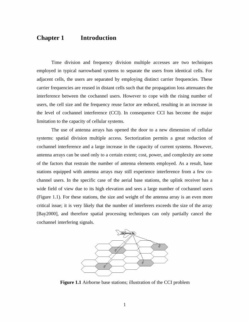
channel users. In the specific case of the aerial base stations, the uplink receiver has a
wide field of view due to its high elevation and sees a large number of cochannel users
(Figure 1.1). For these stations, the size and weight of the antenna array is an even more
critical issue; it is very likely that the number of interferers exceeds the size of the array
[Bay2000], and therefore spatial processing techniques can only partially cancel the
cochannel interfering signals.
Figure 1.1 Airborne base stations; illustration of the CCI problem
P. Barthelemy Chapter 1. Introduction 2
From these considerations, it appears that the use of antenna arrays has not
diminished the need for demodulation schemes robust to CCI. Actually, it is quite the
opposite; by reducing the probability of receiving a large number of interferers (which
can be accounted as noise), spatial processing has accentuated the need for specific
demodulation schemes robust to a small number of interferers [Chi1996].
The goal of this work is to implement a non-coherent demodulation technique for
minimum shift keying (MSK) modulation with improved performance in presence of
CCI. With the success of the pan-European GSM system, MSK has become the most
popular modulation format for narrowband cellular systems. By definition, ‘cochannel‘
users are those who transmit simultaneously with identical carrier frequencies. However,
for frequency shift keying (FSK) modulation, and particularly continuous phase FSK
(which comprises MSK format), the instantaneous frequency of two cochannel signals
also depends on the value of the transmitted symbols. Therefore, over a short observation
interval the instantaneous frequency of the interferer may be different than that of the
user of interest. Thus it may be advantageous to estimate the instantaneous frequency of
the received signal with high resolution techniques; such an estimator could accurately
estimate the dominant frequency of the received signal while rejecting the interference. In
this thesis we have selected a specific frequency estimator and focused on the possible
implementations of this model-based technique for the detection of MSK signals.
Chapter 2 of this thesis presents the MSK modulation format and some of the
most common coherent and non-coherent demodulation schemes for MSK. In Chapter 3,
parametric frequency estimation is introduced and a parametric technique is proposed for
implementing an MSK detector. This model-based technique has been developed by
Kumaresan and Tufts [Kum1982a] and was successfully applied to the demodulation of
AMPS signals [Wel1996]. The implementation of this technique to MSK demodulation
requires important modifications whose details are discussed in Chapter 4. The model-
based scheme is combined with Viterbi equalization, evaluated in AWGN and Rayleigh
fading environments and its performance is compared to the limiter-discriminator and the
coherent Viterbi detector. Chapter 5 presents a study of the CCI rejection capabilities of
the MSK demodulators. Demodulation diversity, first proposed for GMSK in [Las1997a],
is investigated in conjunction with model-based detection. Finally, Chapter 6 concludes
this thesis with a summary and some suggestions for future work.

3
Chapter 2 MSK Signals and Demodulation
Because of its attractive properties, continuous phase modulation (CPM) has seen
wide usage in mobile communications. Minimum shift keying (MSK), which is a form of
CPM, is the modulation format of several wireless standards such as the widely used pan
European GSM (Global System for Mobile). MSK-type signals present a constant
envelope, which permits the use of low complexity non- linear amplifiers and their low
bandwidth spread limits adjacent-channel interference. This spectral efficiency can be
further improved by appropriately pulse-shaping the data as in the case of Gaussian
minimum shift keying (GMSK). Multiple demodulation schemes exist for CPM signals.
When coherent detection is possible good bit-error performance may be achieved,
whereas non-coherent schemes are easily implemented. A major characteristic of MSK is
the inherent presence of inter-symbol interference (ISI) that limits performance of
symbol- level detection schemes. Sequence estimators may be used to mitigate ISI at the
price of increased complexity of the demodulation operation.
2.2 MSK Signals
Minimum shift keying is a special case of continuous-phase frequency shift
keying (CPFSK). Similarly to frequency shift keying (FSK) the binary data is coded by
two frequency tones, but the signal maintains a continuous phase between consecutive
bits. This phase continuity property is the major reason for the higher bandwidth
efficiency of CPFSK as compared to other FSK modulation formats.
The modulated waveform of a binary CPFSK signal with bit period T, carrier
frequency fc and bit energy Eb, may be expressed as [Skl1988][Pro2001]
( ){ }2( ) cos 2 ( ) ( 1)b
c n d n
Es t f a f t nT nT t n T
Tπ ϕ= + − + < ≤ + , (2.1)
where nϕ denotes the phase of the signal at time nT, which is the end of the previous bit.
Also {an} is a polar sequence of ± 1 that encodes the data. Depending on the current
value of {an}, the frequency differs from its median value fc by a quantity of ± fd, called

P. Barthelemy Chapter 2. MSK Signals and Demodulation 4
the frequency deviation. As is obvious from equation (2.1), MSK signals have constant
envelope and continuous phase, which are two major advantages of this modulation
format.
The ratio of 2fd (which is the spacing between the two frequency-tones fc+fd and
fc-fd) to the bit rate is called modulation index and denoted h:
2 dh f T= . (2.2)
The smaller the modulation index, the better is the spectral efficiency [And1986]. In the
case of MSK, the modulation index is equal to 0.5. It is seen that this value for h is the
minimum spacing for which the frequency tones are orthogonal when coherently detected
[Skl1988][Pro2001]. However this minimum deviation does not insure orthogonal
frequency tones when the phase is unknown.
The signal phase nϕ at time nT, is the summation of the phase deviations of all
previously transmitted symbols plus the initial phase 0ϕ of the carrier. Therefore, the
phase of the baseband waveform can be expressed as [Pro2001]: 1
0( ) 2 2 ( ) ( 1)n
LP d k d nk
t f T a f a t nT nT t n Tϕ π π ϕ−
=−∞
= + − + < ≤ +∑ , (2.3)
which can be transformed into a more general expression, for all values of t :
0( ) 2 ( )t
LP it f dτ
ϕ π τ τ ϕ=−∞
= +∫ , (2.4)
where fi(t) is defined as:
( ) ( )i d kk
f t f a g t kT+∞
=−∞
= −∑ , (2.5)
and g(t) is a rectangular pulse of amplitude one and duration T. Using (2.4) as the
expression for the phase, the complex baseband waveform of MSK is:
0( ) exp 2 ( )t
bBB i
Ev t j f d
T τ
π τ τ ϕ=−∞
= +
∫ . (2.6)
In signal processing, fi(t) is known as the instantaneous frequency of the signal at time t
[Boa1992a]. In the case of MSK the instantaneous frequency of the baseband signal (2.5)
is constant by parts, and equals ± fd depending on the value of the current bit an.
A minimum shift keying signal can also be expressed in the form of an offset

P. Barthelemy Chapter 2. MSK Signals and Demodulation 5
quadrature phase shift-keying signal (OQPSK). As shown in [Ben1999] the previous
expressions for the MSK waveform are equivalent to:
( ) ( ) ( ) ( ){ }0 0
2( ) ( ) cos 2 ( ) sin 2b
I c Q c
Es t b t q t nT f t b t q t T nT f t
Tπ ϕ π ϕ= − + − − − + , (2.7)
where
cos ,( ) 2
0 .
tT t T
q t Totherwise
π − ≤ ≤ =
(2.8)
The real and imaginary parts of s(t) carry the information on respectively the even
numbered elements {b2n} and the odd numbered elements {b2n+1}, where {bn} is the data
stream to be transmitted. Namely, 2 1( )Q nb t b += for 2 (2 2)nT t n T< ≤ + whereas
2( )I nb t b= for (2 1) (2 1)n T t n T− < ≤ + . This representation of MSK as a form of OQPSK
results in a simple implementation for the MSK modulator, with block diagram shown on
Figure 2.1. Identification of the OQPSK representation (2.7) and CPFSK representation
(2.1) for MSK gives the relationship between the data streams {an} and {bn} as an=bnbn-1.
Figure 2.1 Block Diagram of an MSK transmitter [Rap1996]
2.2 Gaussian Pulse-Shaping for MSK
Gaussian minimum shift keying (GMSK) is a derivative of MSK with improved
spectral efficiency. Prior to the modulation, the data sequence is shaped by a Gaussian
filter g(t). Then the modulation process is identical to MSK, as described in equations
(2.5) and (2.6).
×
Ccos(2 f t)π
×
bQ(t)
+
+
+ cos( t/(2 ))Tπ
s(t)
bI(t)
BPF fc-h/(2T)
BPF fc+h/(2T)
×
P. Barthelemy Chapter 2. MSK Signals and Demodulation 6
The Gaussian pulse shape has the form of:
2 2( ) ( ) ( )
2 2ln2 ln2B T B T
g t Q t Q tπ π
= − − +
, (2.9)
where the Q function is defined as 2
21( )
2
x
t
Q t e dxπ
∞−
= ∫ . (2.10)
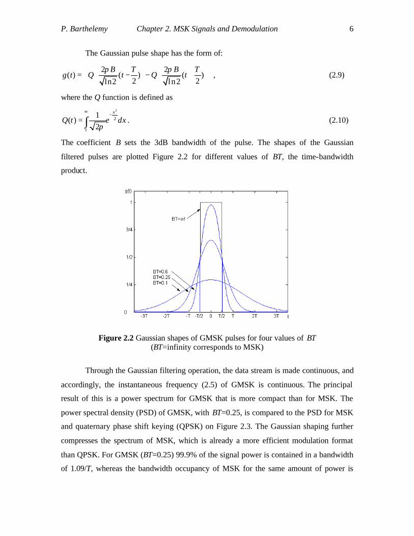
The coefficient B sets the 3dB bandwidth of the pulse. The shapes of the Gaussian
filtered pulses are plotted Figure 2.2 for different values of BT, the time-bandwidth
product.
Figure 2.2 Gaussian shapes of GMSK pulses for four values of BT
(BT=infinity corresponds to MSK)
Through the Gaussian filtering operation, the data stream is made continuous, and
accordingly, the instantaneous frequency (2.5) of GMSK is continuous. The principal
result of this is a power spectrum for GMSK that is more compact than for MSK. The
power spectral density (PSD) of GMSK, with BT=0.25, is compared to the PSD for MSK
and quaternary phase shift keying (QPSK) on Figure 2.3. The Gaussian shaping further
compresses the spectrum of MSK, which is already a more efficient modulation format
than QPSK. For GMSK (BT=0.25) 99.9% of the signal power is contained in a bandwidth
of 1.09/T, whereas the bandwidth occupancy of MSK for the same amount of power is

P. Barthelemy Chapter 2. MSK Signals and Demodulation 7
2.76/T [Rap1996]. The Gaussian shaping attenuates the side- lobes of the spectrum, due to
sharp frequency transitions within the MSK signal. The smaller the BT product chosen,
the smoother are the frequency transitions, and the more compact is the GMSK spectrum.
The spectral efficiency of MSK for different Gaussian and raised-cosine pulse-shapes is
detailed in [And1986].
Figure 2.3 Estimated power spectral density for QPSK, MSK, and GMSK (BT=0.25)
Small values for BT are desirable to achieve good spectral efficiency; however
long durations of the narrow bandwidth pulses result in large inter-symbol interference
(ISI). Whereas MSK signals are full response (the duration of the rectangular pulse shape
does not exceed T) GMSK signals are partial response, and consequently each symbol
interferes with its surrounding neighbors. This inter-symbol interference increases for
decreasing values of BT, and degrades the performance of simple demodulation schemes
based on single symbol decision. GMSK modulation is used in the GSM standard with a
time-bandwidth product equal to BT=0.3, and CDPD (Cellular Digital Packet Data)
employs GMSK with BT=0.5. For what follows, the time-bandwidth product has been
chosen as BT=0.25. As shown in Figure 2.2, for BT=0.25, the Gaussian pulse-shape is
almost zero for 1.5t T> : the current symbol only affects the previous and next symbols.
Therefore to ease the implementation of MSK modulation the pulse may be truncated

P. Barthelemy Chapter 2. MSK Signals and Demodulation 8
outside the time interval [ 1.5 ;1.5 ]T T− with very little degradation of the spectrum
[Pro2001].
The phase of the MSK signal is continuous between consecutive bits. As a result
the signal has some memory of the past data bits. Gaussian pulse shaping further adds
memory to the signal since it introduces ISI. Consequently single-symbol detectors for
GMSK are outperformed by block and sequence estimation schemes. The eye diagram
and phase trajectory of GMSK for a time-bandwidth product of 0.25 are shown Figure
2.4.a and 2.4.b. The effect of ISI is a reduction of the eye opening and an increase in the
number of paths in the eye-diagram and in the phase tree as well.
Figure 2.4 (a) Eye diagram and (b) phase trajectory for GMSK (BT=0.25)
Prior to detection, receivers for MSK and GMSK signals make use of an IF pre-
detection filter that band limits the received signal and therefore reduces the input noise.
The optimum IF filter depends on the shape of the MSK pulse and on the type of
detection that follows the pre-detection filter. Whereas large values for the filter
bandwidth BIF will limit the ISI, the input noise power will be lower for small values of
BIF. For instance, in the case of GMSK signals with BT=0.25 and differential
demodulation, it is shown in [Mur1981] and [Suz1981] that a Gaussian pre-detection
filter with BIFT=0.6 is nearly optimum.
(a) (b)

P. Barthelemy Chapter 2. MSK Signals and Demodulation 9
2.3 Coherent Demodulation
When the carrier phase can be recovered at the receiver, good performance can be
achieved with coherent demodulation. Minimum shift keying can be viewed as a special
case of CPFSK with frequency deviation of h=0.5 or as a form of staggered QPSK with
sinusoidal symbol pulse shaping weighting. These two representations motivate different
structures for the demodulation.
First, the OQPSK representation of MSK may be employed to obtain a simple
coherent demodulator. When seen as an OQPSK signal (2.7), the in-phase and quadrature
parts of the MSK signal are independent and each one carries information of half of the
original bit stream. The in-phase I(t) and quadrature Q(t) parts of the received signal r(t)
may be processed separately [Ben1999] (Figure 2.5). On the in-phase side, the coherent
matched-filter is q(-t) (2.8), whereas for the quadrature part the matched filter is q(T-t).
The output of the in-phase and quadrature matched filters are sampled at even and odd
multiples of T, respectively.
Figure 2.5 Block-diagram of a coherent demodulator for MSK [Las1997a]
An alternative coherent demodulation for MSK is the Viterbi detector. The MSK
signal is now seen as a form of CPFSK (2.1). At time nT the phase of the baseband MSK
signal can only take four values; and possible phase transitions are shown on the trellis
diagram Figure 2.5.a. A phase shift of / 2π+ corresponds to the transmission of the NRZ
symbol +1, whereas symbol –1 results in a phase shift of / 2π− . Under the assumption that
the initial phase of the signal is zero, the MSK signal can also be represented by a two
state tilted trellis diagram (Figure 2.6.b), where state 0 corresponds to the phase zero at
t=(2n+1)T
t=2nT
r(t) ×
×
0cos(2 )cf tπ ϕ+
0-sin(2 )cf tπ ϕ+
I(t)
Q(t) Matched Filter
Matched Filter
BPF
2nb$
2 1nb +$

P. Barthelemy Chapter 2. MSK Signals and Demodulation 10
time t=0, / 2π at time T and so on, whereas state 1 has phase starting from π . The
branch metrics for each of the four possible phase transitions ( , )n t i jϕ → between state
{0,1}i ∈ at time nT and state {0,1}j ∈ at time (n+1)T are calculated as [Pro2001]:
{ }( 1)
( ) ( )cos 2 ( , )n T
n c nnTv i j r t f t t i j dtπ ϕ
+→ = + →∫ . (2.11)
The Viterbi algorithm searches for the path through the trellis with minimum Euclidean
distance from the received signal.
Figure 2.6 (a) Trellis diagram and (b) tilted-phase trellis diagram of MSK
The data sequence of MSK is oftentimes differentially encoded in order to prevent
errors resulting from the possible 180o phase ambiguity in the carrier recovery. MSK with
differential encoding is referred to as DMSK. Coherent receivers have been specifically
developed for DMSK signals. Two of the most common implementations for DMSK are
known as Massey’s receiver and Rimoldi’s receiver [Ben1999, Rim1988].
Offset matched filtering and Viterbi detection are both optimum maximum
likelihood sequence estimators (MLSE) for MSK. Performance of MSK signals with
optimum detection is similar to QPSK [Cou2001] and the bit-error probability is given in
[Rap1996] as:
1.7 bb
o
EP Q
N
=
. (2.12)
A maximum likelihood sequence estimator based on the Viterbi algorithm can
also be constructed for GMSK. However the number of states in the corresponding trellis
is significantly increased: for a pulse-shape g(t) having length LT the optimum Viterbi
(a) (b)

P. Barthelemy Chapter 2. MSK Signals and Demodulation 11
receiver has 2L+1 states [And1986]. In [Mur1981] Murota and Hirade derived the
expression for the bit-error probability of GMSK with coherent detection. For simplicity
GMSK may be detected employing MSK-type coherent demodulators. Inter-symbol
interference introduced by the pre-modulation filter reduces the performance by
approximately 0.3dB relative to the optimum GMSK receiver [Lee1988].
2.4 Non-Coherent Demodulation
Although coherent receivers offer good performance, it is often preferred to avoid
the complexity of the phase synchronization process, which requires the use of phase lock
loops and is vulnerable to fading. As seen previous ly, when non-coherently demodulated,
the frequency spacing of MSK tones is less that the minimum required for orthogonality.
Therefore non-coherent techniques permit inexpensive demodulation of MSK signals, but
with inferior performance in AWGN.
2.4.1 Differential Receiver
The first non-coherent receiver that we examine is the differential detector.
Differential detection consists of comparing the phase of the signal at two different time
instants. The interval between the two observations is usually a multiple of the bit-
duration T, and most common receivers are one bit and two bit differential receivers,
which means that the time-interval for phase comparison is T and 2T, respectively. The
general block diagram of a one-bit differential detector is shown Figure 2.7.
Figure 2.7 Block diagram of a differential detector
Using the complex baseband representation for the received signal and neglecting
the effect of the IF filter, the expression for the differential phase is:
{ }( ) arg ( ) *( )BB BBt r t r t Tϕ∆ = − (2.13)
Predetection Filter
Delay T Phase shift / 2π
ˆnar(t) Phase
ϕ∆t=nT

P. Barthelemy Chapter 2. MSK Signals and Demodulation 12
This differential phase is sampled at time t=nT. From (2.5) the differential phase at time
nT is given by
( 1)( ) 2 ( )
nT
d k noiset n Tk
nT f a g t kTϕ π ϕ+∞
= −=−∞
∆ = − + ∆∑∫ , (2.14)
where noiseϕ∆ corresponds to the effect of the additive noise. For MSK, the phase
difference only depends on the value of the current bit, and the expression reduces to:
( )2 n noisenT aπ
ϕ ϕ∆ = + ∆ . (2.15)
In the case of GMSK with pulse-shape truncated for 1.5t T> , the decision statistic
depends on three consecutive bits [Las1997a]:
1 1 0 1 1( ) ( )2 n n n noisenT a a aπ
ϕ α α α ϕ− − + +∆ = + + + ∆ . (2.16)
For BT = 0.25 the contributions of the three bits are weighted by 0 =0.589α and
-1 +1= =0.205α α .
Two bit differential detection is presented in [Sim1984]. The decision is made
using the value of the difference between the signal phase at time t and t+2T. Two or
three-bit differential detection have improved performances as compared to one-bit
differential detection [Yon1988].
2.4.2 Discriminator Receiver
Similarly to frequency shift keying signals, MSK signals can be demodulated with
limiter-discriminator receivers. The information content of the received signal is
imbedded in its frequency, which is the derivative of the phase. This derivation can be
performed employing a discriminator. The output of the discriminator is integrated over
the bit duration T, for which the frequency is constant, and sampled at time t=nT. Finally,
the decision statistic of the discriminator may be expressed similarly to (2.15) [And1986].
The block-diagram of the limiter-discriminator receiver is shown Figure 2.8. Prior to the
discrimination operation, the signal is passed through a limiter that restores the constant
envelop of the signal.

P. Barthelemy Chapter 2. MSK Signals and Demodulation 13
Figure 2.8 Block diagram of a limiter discriminator
For MSK (h=0.5), differential and discriminator detectors have identical
performance in AWGN [Sim1983]. However, in the presence of co-channel interference,
random FM noise or Rayleigh fading, the performance of differential detection and
limiter discrimination slightly differ [Las1997a].
2.4.3 Non-Coherent Sequence Detection
The ease of implementation of non-coherent demodulators for MSK makes these
techniques very attractive. However differential and limiter-discriminator detection suffer
from the large ISI introduced by the IF pre-detection filter and also by the partial
response pulse shaping for GMSK. Two approaches have been proposed to compensate
this ISI. Hirono, Miki and Murota [Hir1984] developed a multilevel detection that
employs decision feedback equalization (DFE). DFE may be used after a limiter-
discriminator [Ada1988a] or with differential detection [Yon1988]. In both cases the
output of the post-detection filter is corrected by the weighted va lues of the previously
decided bits. Assuming that the SNR is large and that the pre-detection filter introduces
no ISI, the decision statistic for GMSK after 1-bit differential detection and with 1-bit
DFE can be written as:
{ }( )1 1 1 0 1 1ˆ( )2 n n n n noisenT a a a aπ
ϕ α α α ϕ− − − + +∆ = − + + + ∆ . (2.17)
And if an-1 has been correctly detected then
( )0 1 1( )2 n n noisenT a aπ
ϕ α α ϕ+ +∆ = + + ∆ . (2.18)
As compared to (2.16), the effect of the previous bit has been cancelled, and thus the
demodulation suffers from only half of the original ISI. When the pulse spreads over
more symbols, ISI from bits earlier than an-1 can also be removed with 2-bit or 3-bit DFE.
Limiter Discriminator LPF ˆna
t=nT r(t) Predetection
Filter

P. Barthelemy Chapter 2. MSK Signals and Demodulation 14
The second method, proposed by Chung [Chu1984], makes use of post-detection
maximum-likelihood sequence estimation (MLSE) or Viterbi detection. Since the noise at
the output of the discriminator or the differential detector is not gaussian, a post-detection
sequence estimation based on the Viterbi algorithm is not MLSE in the strict sense
[Tun1994]. Also the non-Gaussian nature of noise at the input of the Viterbi detector
prevents a rigorous analytical derivation of performance for the non-coherent sequence
detector.
In [Chu1984], two-states trellises were first considered. Then Viterbi detectors for
four states or more have been investigated to improve non-coherent detection [Iwa1995].
The eye-diagram of the signal at the output of the discriminator is shown in Figure 2.9 for
BT=0.25 and BIFT=0.6. The Gaussian pulse shape has length 3T and the IF filter has
length 2T. As a result the current symbol interferes only with the two previous and the
two subsequent symbols [Iwa1995]. The memory of the signal at the input of the
discriminator is L=5T, and the total number of possible paths is equal to 2L=32; and the
trellis diagram that represents all the transitions has 16 states. The block diagram of a
non-coherent sequence detector with limiter discrimination is represented Figure 2.10.
Figure 2.9 Eye pattern of the discriminator output for GMSK (BT=0.25) and Gaussian
pre-detection filter (BIFT=0.6)

P. Barthelemy Chapter 2. MSK Signals and Demodulation 15
Figure 2.10 Block diagram of a sequence estimation scheme with limiter-discriminator
detection.
Sequence estimation after the non-coherent detector diminishes the effect of ISI.
Therefore IF filters with narrower bandwidth (and longer time duration) may be used to
reduce the input noise, while ISI is compensated using augmented trellises [Iwa1995].
Large gains may thus be obtained with the non-coherent schemes, but with an increased
complexity due to the large trellises employed in the sequence estimation process.
2.5 Summary
In this chapter, fundamentals of minimum shift keying signals have been
presented along with some possible demodulation schemes. MSK is a form of frequency
modulation. Coherent receiver mainly exploit the phase continuity property of MSK
signals, while non-coherent receivers function by estimating the frequency of the signal
and then comparing the estimate to a zero threshold. The conventional frequency
detectors, such as the differential detector and the limiter-discriminator however, suffer
from the small spacing between MSK frequency tones and have poor performance in
noise corrupted environments. This limited performance is further degraded in the
presence of co-channel interferers. As seen in Chapter 1, the capacity of a narrowband
system is limited by co-channel interference. Therefore, robust performance in co-
channel interference is a central matter, when choosing a demodulation scheme for MSK.
In the next chapter improved frequency estimation techniques are investigated as possible
substitutes to the differential detector and discriminator.
h1(-t)
h2(-t)
h32(-t)
L&D r(t)
Predetection Filter
Vite
rbi P
roce
ssor
ˆna
t=nT

16
Chapter 3 Parametric Frequency Estimation
3.1 Overview on Frequency Estimation
Spectral estimation of a digital signal, and especially determination of its
dominant frequencies is a major issue for a large number of communication problems.
Frequency estimation techniques have been studied for use in speech processing,
demodulation of analog FM signals and digital FSK signals, and for angle of arrival
estimation in adaptive antenna arrays. When the purpose is to demodulate MSK signals in
an interference- limited environment, the need is to find a spectral estimator that is able to
distinguish between very closely spaced frequency tones and that precisely locates the
peaks of the signal spectrum.
Spectral estimation techniques can be grouped into two categories: parametric
techniques, also called model-based, and non-parametric techniques. Whereas non-
parametric techniques make no assumption about the form of the signal, parametric
estimators match the signal to a given model and make use of this model to estimate the
signal spectrum. In addition to the classical Fourier analysis, the class of non-parametric
techniques has recently been enriched with new time-frequency techniques such as the
Wigner-Ville distribution [Boa1992b]. Meanwhile parametric techniques based on
autoregressive modeling and subspace decomposition have been successfully applied to
diverse applications.
The performance of the different techniques heavily depends on the type of signal
that is to be estimated. This is even more obvious in the case of model-based techniques
where performance relies on how closely the assumed model approximates the observed
signal and where an inappropriate model could lead to irreducible error in the estimation.
Parametric spectral estimation is a three steps process. First, a model for the signal is
chosen. Then the model parameters are estimated such that the model accurately fits the
observed signal. Finally the spectrum of the model is calculated and peaks of this
spectrum are identified as the dominant frequency tones of the observed signal. Through
the choice of a model, parametric techniques exploit some a-priori knowledge about the

P. Barthelemy Parametric Frequency Estimation 17
signal structure. Therefore provided that the model is well chosen, parametric techniques
can achieve higher accuracy than non-parametric techniques [Kay1988]. Typically for
stationary signals a model-based technique can resolve frequency tones separated by only
1/(2N), where N is the number of data points available [Wel1996], which is twice better
than resolution of the Fourier spectrum. For this reason parametric techniques are
preferable to time-frequency analysis.
Among possible parametric techniques, rational spectral modeling techniques
(and especially autoregressive modeling) are of prime interest due to their good
performance and the ease of estimation of the model parameters. For the specific case of
autoregressive frequency estimation, estimates of the parameters are typically found via
linear prediction techniques. Moreover, accuracy of the autoregressive estimates can be
significantly increased by taking advantage of the properties of the autocorrelation matrix
eigen-decomposition [Kum1982b].
3.2 The Autoregressive Model
The choice of a good model for the observed signal is essential to ensure accurate
frequency estimates. Techniques based on autoregressive (AR) modeling may
successfully approximate peaks of the power spectrum for stationary signals [Kay1988].
Also as shown in Chapter 2, MSK signals have constant frequency over the duration of
one bit. Therefore over a bit period, the signal received by a MSK base-station will
mainly consist of one dominant frequency tone from the user of interest, white Gaussian
noise, and possibly other interfering MSK signals resulting in some additional peaks in
the power spectrum distribution. This received signal can be accurately modeled as an
AR process.
An autoregressive process of order p is a linear stochastic process with outcome
depending on the only p previous outcomes. If xAR(n) is an AR(p) signal then there exists
a set of p coefficients {a1,...,ap} such that:
1
( ) ( ) ( )P
AR k ARk
x n a x n p w n=
= × − +∑ , (3.1)

P. Barthelemy Parametric Frequency Estimation 18
where w(n) is a white Gaussian noise with variance 2Wσ . AR signals can also be
represented as the output of a linear filter with input white Gaussian no ise W(z) and
transfer- function H(z):
( ) ( ) ( )ARX z H z W z= . (3.2)
Identification of equation (3.1) and (3.2) gives the expression for the transfer- function:
1
1( )
1p
kk
k
H za z −
=
=− ∑
. (3.3)
The power spectral density SX(f) of the random process xAR(n) is defined as the Fourier
transform of its autocorrelation function. If xAR(n) is given by (3.2) with H(z) being a
linear process, SX(f) can also be expressed as the product of the modulus of H(z) squared
and the power spectral density of the noise, which has amplitude 2Wσ [Clar1993]:
( ) ( ) ( )22
2 22
2
1
1
f f wX W
pk f
kk
S f S e H e
a e
π π
π
σ
−
=
= =
−∑. (3.4)
When an observed signal x(n) is to be estimated via AR(p) modeling, the
parameters {a1,…,ap} are chosen so that the AR model best represents the signal. Then
an estimate of the power spectrum of the signal is given by (3.4). The noise power 2Wσ is
constant over all frequencies and does not need to be estimated. Therefore the problem of
estimating the power spectrum has been transformed into a problem of parameter
estimation.
3.3 AR Parameter Estimation
3.3.1 Linear Prediction
The nth sample of an autoregressive process linearly depends on its p previous
values (3.1). Hence, for a complex sequence that may be modeled by an AR(p) signal, an
estimate of its sample x(n) can be found as a linear combination of {x(n-p),…,x(n-1)}
using some weighting coefficients {c1,…,cp}, called the prediction filter:

P. Barthelemy Parametric Frequency Estimation 19
1
( ) ( )P
kk
x n c x n k=
= × −∑) . (3.5)
The forward prediction differs from the observed value by the prediction error ( )nε . This
error ( )nε is a measure for the accuracy of the prediction.
1
( ) ( ) ( ) ( ) ( )P
kk
n x n x n x n c x n kε=
= − = − × −∑) (3.6)
Parametric estimation via linear prediction consists of finding the set of
coefficients {c1,…,cp} such that the power of the prediction error is minimized. This is
the least square solution for the linear prediction equation (3.5). If the signal is strictly
AR and of same order of the prediction, then the AR parameters form a set of prediction
coefficients with prediction error equal to w(n) and error power 2Wσ , which has been
proved to be the minimum achievable power for the prediction error [Hay1996]. This is
in contrast to the problem of parameter estimation where the true AR coefficients are
unknown but approximated by the least square solution of the linear prediction problem.
At this point it might be helpful to consider the noiseless case, where the signal of
interest is only composed of M complex sinusoids. It is easily shown that such a signal
can be exactly predicted with a prediction filter of order p equal to M. For instance a
single sinusoid of frequency f1 will yield a next sample equal to its current value but with
phase shifted by 12 fπ : in other words ( )1 1exp 2c j fπ= . In the case of two complex
sinusoids with normalized frequencies f1 and f2, the second order prediction coefficients
can be found as ( ) ( )1 1 2exp 2 exp 2c j f j fπ π= + and ( )( )2 1 2exp 2c j f fπ= − + with zero
prediction error. However, in the noisy case a prediction with order equal to the number
of pure sinusoids present in the signal is not always desirable. The presence of noise at a
high level can be attributed to an increase in the signal complexity and consequently
linear prediction of order higher than M may describe the signal more accurately.
3.2.2 Yule-Walker Equations
The general least square (LS) solution for the linear prediction problem is derived
in this section. Following (3.3) the average power of the prediction error can be written as

P. Barthelemy Parametric Frequency Estimation 20
{ }2
2
1
( ) ( ) ( )P
kk
P E n E x n c x n kε ε=
= = − × −
∑ . (3.7)
Introducing the autocorrelation function rXX(k), another expression for this mean square
prediction error is
( )0 H H HXX XX XX XXP r r c c r c R cε = − − + , (3.8)
where the autocorrelation function is defined for k ranging from 0 to p as
( ) { }( ) *( )XXr k E x n x n k= + , (3.9)
and the autocorrelation matrix and autocorrelation vector have the form of respectively
( ) ( ) ( )( ) ( ) ( )
( ) ( ) ( )
0 * 1 * 11 0 * 2
1 2 0
XX XX XX
XX XX XXXX
XX XX XX
r r r pr r r p
R
r p r p r
− − =
− −
LL
M M O ML
,
( )( )
( )
12
XX
XXXX
XX
rr
r
r p
=
M . (3.10)
After differentiation of equation (3.8) with respect to the complex vector c of prediction
coefficients, the minimum prediction error power is found by setting 0Pcε∂
=∂
, which is
equivalent to [Vas2000]:
0XX XXR c r− = . (3.11)
This relation between the least square prediction coefficients and the autocorrelation
function is the matrix form of the Yule-Walker equations for AR modeling [Kay1988].
When RXX is invertible, the solution for the Yule-Walker equations is simply 1
XX XXc R r−= . (3.12)
Since the true autocorrelation function of the signal is unknown, rXX(k) (3.9) must
be estimated from the available samples. As a consequence, the general least-square
solution in (3.12) leads to several parametric methods, depending on the choice for the
approximation of the autocorrelation function.
A simple approximation of rXX(k) is given by the following expression:
1
1( ) ( ) * ( )
N
XXn
r k x n x n kN =
= +∑ , (3.13)

P. Barthelemy Parametric Frequency Estimation 21
where x(n) is assumed to be zero outside the observation interval. The resulting AR
model is called the autocorrelation method. Due to its relatively poor spectral estimation
other AR techniques described below are usually preferred to the autocorrelation method.
3.3.3 Covariance Method
If a total of N>p consecutive data samples are available, then N-p forward
prediction equations analogous to (3.6) can be written. Also, as the observed signal is
assumed to be stationary over those N samples, the prediction coefficients are unchanged
for these N-p equations. The resulting set of equation can be written in matrix form:
{
1
2
(1) ( 1) ( ) ( 1) (1)(2) ( 2) ( 1) ( ) (2)
( ) ( ) ( 1) ( 2) ( ) p
cx p x p x p xcx p x p x p x
cN p x N x N x N x N p
cx X
εε
ε
ε
+ − + + = − − − − −
= −
LL
MM M M M O ML14243 14243 14444444244444443
. (3.14)
As seen above, a good prediction should result in an estimate with minimum
average error power. If Pε is the mean power of the N-p forward prediction errors then
( )1 1H H H H H H HP x x x Xc c X x c X XcN p N pε ε ε= = − − +
− −. (3.15)
When XHX is invertible, the minimum of Pε is found when [Sto1997]
( ) ( )1H Hc X x X X X x−+= = , (3.16)
with X+ defined as the pseudo- inverse or Moore-Penrose generalized inverse of X. This
least square solution for the AR model parameters is often referred to as the forward-
prediction solution, the covariance method or extended Prony’s method. Replacing the
autocorrelation matrix RXX and autocorrelation vector rXX by respectively XHX and XHx,
then the covariance method (3.16) represents an approximate solution for the Yule-
Walker problem (3.12), and an alternative to the autocorrelation method.
Resulting from their similarity, the autocorrelation and covariance methods have
comparable performance for large values of N. However, for a smaller number of
samples, the autocorrelation and covariance methods have a slightly different behavior
[Sto1997]. In the case of the modified covariance method, the AR model parameters

P. Barthelemy Parametric Frequency Estimation 22
obtained may be unstable, whereas the autocorrelation method insures the stability of the
model. Yet unstable AR parameters are very unlikely and, what is more, stability is not
an issue for the frequency estimation problem..
Also for small values of N, the covariance method is seen to outperform the
autocorrelation method. The underlying assumption made by the autocorrelation method
is that the signal equals zero outside the observation interval [Hay1996]. This incorrect
assumption results in end effects and degrades the performance when the number of
samples N is small. From equation (3.13) the function rXX(k), k={0,…,N-1}, is averaged
over N lag products for the autocorrelation method, k of which are zero [Kay1988].
Consequently the estimated autocorrelation function may become unreliable for k close to
N. By contrast the covariance method estimates each autocorrelation value rXX(k),
k={0,…,N-p} as the mean of a constant number of p measurements, making no
assumption for the signal outside the observation interval. Yet for k close to zero the
covariance method does not employ all possible N-k lag products to estimate the
autocorrelation function, which is the case for the autocorrelation method and also for the
modified covariance method.
3.3.4 Modified Covariance Method
Forward prediction consists of predicting the sample x(n) from the p previous
observations {x(n-p),…,x(n-1)}. Alternatively, if {x(n+1),…,x(n+p)} are known it may
be possible to guess the value of the previous data sample x(n); this procedure is called
backward prediction. While prediction of the past may not seem very pertinent, backward
prediction is of great help when the purpose is to estimate the AR parameters of a signal.
The backward linear prediction of x(n) with prediction coefficients {b1,...,bp}may be
expressed as:
1
( ) ( )P
kk
x n b x n k=
= × +∑) . (3.17)
The forward (3.5) and backward (3.17) linear predictions are similar except that
the data coefficients are reversed in time. As a result, the optimum solution for the
backward vector coefficients {b1,…,bp} is directly related to the optimum forward

P. Barthelemy Parametric Frequency Estimation 23
coefficients {c1,…,cp} and more precisely {c1,…,cp} is the complex conjugate of the
reversed backward filter {bp,…,b1} [Kay1988].
While (N-p) equations for the forward prediction error were written in (3.14), an
additional set of (N-p) backward equations can be derived from N samples when the order
of prediction is p. The combination of the 2(N-p) equations gives:
(1) ( 1) ( ) ( 1) (1)
(2) ( 2) ( 1) ( ) (2)
( ) ( ) ( 1) ( 2) ((1) *(1)(2) *(2)
( ) *( )
F
F
F
B
B
B
FBLPFBLP
x p x p x p x
x p x p x p x
N p x N x N x N x N
xx
N p x N p
x
εε
εεε
ε
ε
+ − + − − − − − = −
− −
LL
M M M M O ML
M M14424431442443
1
2)
*(2) *(3) *( 1)*(3) *(4) *( 2)
* ( 1) *( 2) *( )
p
FBLP
c
cp
x x x pcx x x p
x N p x N p x N
X
+
+
− + − +
MLL
M M O ML144444444424444444443
(3.18)
The solution that minimizes the power of the total prediction error FBLPε is
identical to the covariance method (3.16) except that data vector x and data matrix X are
now of respective dimensions 2(N-p) and 2(N-p)×p as defined above (3.18). This
procedure is called the modified covariance or forward-backward method [The1992].
Solving for the model parameters by way of the modified covariance method minimizes
the sum of the forward and backward error power and leads to a significant increase in
performance. As the autocorrelation function is averaged over a number of lag products
larger than the initial covariance method, variance of the estimated parameters is reduced.
Frequency estimates obtained from the modified covariance method present
various advantages such as a relatively low bias, a small dependence on the initial phase
and a high resolution at moderate SNR [Kay1988]. This makes the modified covariance a
good candidate for the present application. However, the performance of this method
degrades for low SNR, which motivates the use of advanced noise reduction techniques.

P. Barthelemy Parametric Frequency Estimation 24
3.4 Subspace Decomposition of the Autocorrelation Matrix
3.4.1 Properties of the Autocorrelation Matrix
Each of the AR modeling techniques presented above relies on an estimate of the
autocorrelation matrix. For reasonable signal to noise ratio this estimate is accurate and
parameters precisely fit the signal. However, when the noise power is high the resulting
autocorrelation matrix and prediction filter may contain a large portion of the noise. To
attenuate the effect of noise and improve the AR methods, subspace decomposition is
performed on the autocorrelation matrix.
The use of subspace decomposition of the autocorrelation matrix for frequency
estimation was initially employed in the Pisarenko Harmonic Decomposition [Kay1988].
This technique has been improved to give the Multiple Signal Classification method
(MUSIC) and more recently the Estimation of Signal Parameters via Rotational
Invariance techniques (ESPRIT) [The1992]. In these techniques, eigenvalue
decomposition of the autocorrelation matrix is performed to determine directions of the
signal and noise spaces. In the case of AR modeling, the eigenvalue decomposition may
be used as a noise reduction technique for the autocorrelation matrix [Kum1982a].
For a signal composed of M frequency tones with additive white Gaussian noise it
can be shown that the theoretical L×L autocorrelation matrix is the summation of a signal
autocorrelation matrix and a noise autocorrelation matrix with the following properties
[Kay1988]. The first matrix has rank M. Each of its M non-zero eigenvalues is equal to
the power of one of the M sinusoids. The corresponding M eigenvectors span the signal
space. The second matrix is full rank and its L eigenvalues are equal to the noise power 2
Wσ . The result is a total autocorrelation matrix that has M principal eigenvalues
{ }1,..., Mλ λ and a remaining L-M almost zero eigenvalues { }1,...,M Lλ λ+ . Moreover, the
noise space spanned by the L-M eigenvectors {eM+1,…,eL} corresponding to the L-M
smallest eigenvalues is orthogonal to the signal space [The1992].
With these notations the eigen-decomposition of the autocorrelation matrix is:
1 1 1
L M LH H H
XX i i i i i i i i ii i i M
signal space noisespace
R e e e e e eλ λ λ= = = +
= = +∑ ∑ ∑14243 14243
. (3.19)

P. Barthelemy Parametric Frequency Estimation 25
As the noise space is orthogonal to the signal space and consequently does not contain
any relevant information on the signal, the autocorrelation matrix can be approximated as
µ1
MH
XX i i ii
R e eλ=
= ∑ . (3.20)
This reduced rank approximation of the autocorrelation matrix will then be used instead
of the original autocorrelation matrix to estimate the AR parameters in (3.12). The overall
effect of this subspace technique is a decrease in the noise power of the estimated
parameters. Consequently at low SNR much higher frequency resolution can be achieved
as compared to the simple linear prediction techniques.
3.4.2 Kumaresan and Tufts’s Method
Work performed by Kumaresan and Tufts has contributed to the improvement of
the modified covariance method [Kum1982a][Kum1982b] through an efficient method to
combine forward-backward linear prediction and the principal component approach.
Recall that the modified covariance method minimizes the sum of the forward and
backward predic tion errors and estimates the autocorrelation matrix by RXX=XHX, where
X is defined as in equation (3.18). For further improvement of the modified covariance
method, RXX can be replaced by its reduced rank approximation containing only M
dominant components. The principal component of the p×p autocorrelation matrix may
be obtained by eigenvalue decomposition. But for large values of prediction order,
computation of the principal components via eigen-decomposition may become
impractical. However Kumaresan and Tufts have shown that this complex decomposition
of the autocorrelation matrix can be avoided and replaced by a simpler operation on the
data matrix X while preserving the advantages of subspace decomposition [Kum1982b].
For the 2(N-p)×p data matrix X the ordinary singular value decomposition (SVD)
is the factorization of X into three matrices U, Σ and V such that [Jen1991] HX U V= Σ , (3.21)
and where Σ is a 2(N-p)×p diagonal matrix with diagonal elements iσ known as the
singular values of X. Then XHX can be expressed as 2
( )H H H H HX X U V U V V V= Σ Σ = Σ . (3.22)

P. Barthelemy Parametric Frequency Estimation 26
Identification of the expressions for XHX in (3.22) and RXX in (3.19) leads to the
conclusion that the eigenvalues of the autocorrelation matrix are simply the norm squared
of the singular values of X. Therefore there is a one to one correspondence between the
principal components of RXX and the principal singular values of X, and rank reduction of
the autocorrelation matrix is equivalent to rank reduction of the data matrix X,
µ1
MH
i i ii
X u vσ=
= ∑ . (3.23)
The solution for the AR parameters may be obtained by multiplying the pseudo
inverse of X by the data vector x (3.16). Using the singular value decomposition of X, it is
seen that the pseudo- inverse X+ is equal to [Jen1991]:
( ) 1H H HX X X X V U−+ += = Σ . (3.24)
The pseudo- invert of Σ is a p×2(N-p) diagonal matrix with diagonal elements iσ + equal
to 1iσ − if iσ is non-zero or zero otherwise. If the data matrix is replaced by its reduced
rank approximation (3.23), the only M dominant singular values are kept and the pseudo-
inverse X+ is approximated as
µ1
1MH
i ii i
X v uσ
+
=
= ∑ . (3.25)
In summary Kumaresan and Tufts’s method estimates the AR parameters as [Kum1982a]
µ1
1MH
i ii i
c X x vu xσ
+
=
= = ∑$ . (3.26)
Specifically, when the signal of interest is a simple sinusoid imbedded in white Gaussian
noise, the principal component AR estimator consists in
1 11
1 HPCc v u x
σ= . (3.27)
With Kumaresan and Tufts’s method, computation of the eigen-decomposition of
the p×p autocorrelation matrix is replaced by a singular value decomposition of the
2( )N p p− × data matrix X, which for practical values of p may save a significant
amount of computation while fully exploiting the subspace decomposition.

P. Barthelemy Parametric Frequency Estimation 27
3.5 Frequency Estimation by AR Modeling
3.5.1 Polynomial Rooting
Linear prediction and eigenvalue-decomposition techniques have been reviewed
as a mean to estimate the AR parameters. One of the motivations for obtaining the AR(p)
parameters is to analyze the direct relationship between these parameters and the
spectrum of the autoregressive signal. From (3.4), an estimate of the observed signal
spectrum is, within a multiplicative constant, the magnitude of the frequency response of
filter H(z), where the true AR parameters {a1,…,ap} are now replaced by their estimates
{c1,…,cp}.
The observed signal is assumed to be composed of M pure sinusoids, which are to
be estimated, and additive noise. Provided that the power of these sinusoids is high
enough compared to the noise level, frequency components of the signal will result in
peaks in the estimated power spectrum. To get the frequency of these peaks, the response
of H(z) can be evaluated for a fine grid of frequencies. Then the M local maximums with
highest power are chosen as estimates for the frequency components. To obtain good
accuracy for the peak location, the frequency response of H(z) must be computed for a
large number of points; therefore precise estimation of the components requires
numerous calculations.
Polynomial rooting is an alternative method for estimating the frequency
components, that is sometimes less computationally intensive. Peaks of the spectrum are
found when the polynomial denominator of H(z) is close to zero. Therefore there is a
direct correspondence between the roots of the polynomial {1,-c1,…,-cp} and peaks of the
filter response. In the complex plane, the angle of the poles corresponds to the peak
frequencies of the spectrum and closeness of the poles to the unit circle gives an estimate
of the magnitude of the spectrum at these frequencies. The correspondence between the
location of the poles and the peak frequencies of the power spectrum is clearly seen by
comparison of the normalized frequency response of the digital filter H(z) (Figure 3.1.a)
with position of its nine poles (Figure 3.1.a), obtained for a signal composed of four
sinusoids in AWGN. Angles of the poles have been represented as vertical lines in the
power spectrum plot (Figure 3.1.a) and perfectly match the position of the peaks.

P. Barthelemy Parametric Frequency Estimation 28
Figure 3.1 (a) Estimated AR spectrum and (b) location of the nine roots of the filter denominator obtained for a signal composed of four sinusoids in AWGN
Thus frequency estimates of the M sinusoids may either be chosen as the peak of
the estimated spectrum or, equivalently, as the angles of the M poles closest to the unit
circle, obtained by finding the roots of {1,-c1,…,-cp}. Moreover the pole-zero plot gives a
convenient visualization of the effect of the different AR techniques, and in particular it
provides some insight for the choice of the model order.
3.5.2 Model Order Selection
The choice of an efficient parametric method is important, and accuracy of the
frequency estimate will primarily depend on the selection of an appropriate order p for
the AR model. It was previously seen that for a noiseless signal a prediction order equal
to the number M of sinusoids present is sufficient. However, when noise becomes
significant, M is no longer the optimum value for the prediction order p.
To illustrate the effect of noise, a signal composed of two equal-power complex
sinusoids is considered. The two sinusoids have initial phase equal to zero and
normalized frequencies centered on zero and spacing of 1/2N, with N equal to 25. The
signal is corrupted by additive white Gaussian noise. Pole locations obtained for multiple
trials of the modified covariance method are shown on Figure 3.2.a for a model order of
p=M=2 and Figure 3.2.b for p=8. These figures show that the separation of the two
frequency tones is not possible when p and M are equal. Actually, in the case p=M, one of
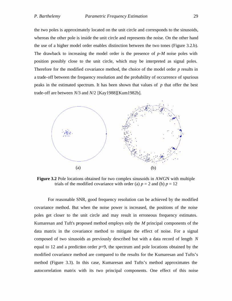
P. Barthelemy Parametric Frequency Estimation 29
the two poles is approximately located on the unit circle and corresponds to the sinusoids,
whereas the other pole is inside the unit circle and represents the noise. On the other hand
the use of a higher model order enables distinction between the two tones (Figure 3.2.b).
The drawback to increasing the model order is the presence of p-M noise poles with
position possibly close to the unit circle, which may be interpreted as signal poles.
Therefore for the modified covariance method, the choice of the model order p results in
a trade-off between the frequency resolution and the probability of occurrence of spurious
peaks in the estimated spectrum. It has been shown that values of p that offer the best
trade-off are between N/3 and N/2 [Kay1988][Kum1982b].
Figure 3.2 Pole locations obtained for two complex sinusoids in AWGN with multiple trials of the modified covariance with order (a) p = 2 and (b) p = 12
For reasonable SNR, good frequency resolution can be achieved by the modified
covariance method. But when the noise power is increased, the positions of the noise
poles get closer to the unit circle and may result in erroneous frequency estimates.
Kumaresan and Tuft's proposed method employs only the M principal components of the
data matrix in the covariance method to mitigate the effect of noise. For a signal
composed of two sinusoids as previously described but with a data record of length N
equal to 12 and a prediction order p=9, the spectrum and pole locations obtained by the
modified covariance method are compared to the results for the Kumaresan and Tufts’s
method (Figure 3.3). In this case, Kumaresan and Tufts’s method approximates the
autocorrelation matrix with its two principal components. One effect of this noise
(a) (b)

P. Barthelemy Parametric Frequency Estimation 30
reduction is the disappearance of the spurious peaks in the estimated spectrum, and
accordingly, noise poles get more distant from the unit circle in the pole-zero plot. The
chance of misinterpreting a noise pole as a signal pole is thus reduced while the
frequency resolution is increased, because the order of the model can be higher than for
the modified covariance method.
Figure 3.3 Comparison of the estimated spectrum and pole locations obtained for two complex sinusoids in AWGN with (a,b) the forward-backward autocorrelation matrix and
(c,d) its reduced-rank approximation (two principal components). N=12 and p=9.
The optimum value for p was experimentally found to be 3N/4 [Kum1982b],
whereas the number of components selected in the SVD decomposition depends on M.
Although the number of sinusoids present in the signal may not be exactly known in
(a) (b)
(c) (d)

P. Barthelemy Parametric Frequency Estimation 31
practice, in many cases of interest only one or two dominant components are of interest
and other sinusoids will have lower power. Therefore in most cases the only one or two
principal components are kept, no matter what the number of interfering sinusoids may
be.
3.6 Summary
In this chapter some high-resolution frequency estimation techniques have been
presented as possible candidates for implementation as a minimum shift keying
demodulator. As minimum shift keying is a form of frequency modulation (with
continuous phase) the received signal may be detected based on the estimation of its
instantaneous frequency. However, due to the minimum frequency deviation of MSK,
only high-resolution estimators, such as the autoregressive frequency estimators, are of
interest.
AR modeling leads to the Yule-Walker equations. The autocorrelation, the
covariance and the modified covariance methods are alternative solutions for this
problem. Then the properties of the eigen-decomposition of the autocorrelation matrix
and their applications to noise reduction have been overviewed. Finally two techniques
were presented to obtain the instantaneous frequency of the signal from the estimated AR
parameters.
Kumaresan and Tufts principal component approach combines parametric
modeling and subspace decomposition. The advantages of this method are its low bias,
similarly to the modified covariance method, a good resistance to noise due to the
subspace decomposition, and a reasonable complexity, resulting from the decomposition
of the data matrix rather than the autocorrelation matrix.
A non-coherent demodulator for MSK signals must be able to distinguish between
two frequency tones with spacing fS/(2N). Also, in presence of co-channel interferers, the
demodulation of the strong signal requires further accuracy of the spectral estimator.
These considerations have motivated our choice to implement a MSK demodulator based
on the principal component method developed by Kumaresan and Tufts [Kum1982b].

32
Chapter 4 Implementation of a Model Based Demodulator Parametric frequency estimation has been proposed in [Wel1996] as a
demodulation technique for the Advanced Mobile Phone System (AMPS). AMPS signals
are frequency modulated; therefore the demodulation of AMPS signals is a frequency
estimation problem. In particular, the principal component technique, as presented in
Chapter 3, is shown in [Wel1996] to offer good performance as a demodulator for AMPS
and to be robust to co-channel interference. Those results have motivated our choice to
adapt this frequency estimation technique to the demodulation of digital FM signals, and
especially of MSK-types signals.
The implementation of a model-based (MB) demodulator to detect MSK signals
is investigated in this chapter. First, a simple demodulation scheme based on Kumaresan
and Tufts method is proposed for the detection. Exploiting a-priori information on the
form of the received signal, and employing pre-detection filtering and post-detection
sequence estimation, the performance of this model-based scheme can be significantly
enhanced. Finally, the performance of the improved model-based demodulator is assessed
for the AWGN channel and for the flat fading channels. Simulation results of the MB
technique are compared to the limiter-discriminator and the coherent Viterbi detector.
4.1 Performance of the Parametric Frequency Estimators
In this section the performance of the parametric frequency estimators presented
in chapter 3 are evaluated for a simple scenario. The signal is composed of a complex
sinusoid with normalized frequency fi equal to 0.5 and additive white Gaussian noise with
variance 2wσ .
{ }( ) exp 2 ( ) ( )i is n A j nf w nπ ϕ= + + (4.1)
The length of the data record is N=8 samples, which is a typical value for the over-
sampling of GMSK receivers. The SNR is defined here as the ratio of the signal power
2A to the noise power 2wσ .

P. Barthelemy Chapter 4. Implementation of a Model Based Demodulator 33
The ability of a technique to accurately estimate the instantaneous frequency of
the signal is measured by the mean square error [Kay1993]:
{ } { }2
i i iMSE f E f f= −) )
, (4.2)
where if)
is an estimate of the instantaneous frequency if . If the estimator is unbiased the
mean square error is simply the variance of the estimator.
Provided that the probability density function p(x,f i) of the quantity to be
estimated (the instantaneous frequency in our case) satisfies some regularity conditions
[Kay1993], the Cramer-Rao lower bound (CRLB) for an unbiased estimator is defined as:
{ } 2
1
ln ( , )i
i
i
MSE fp x f
Ef
≥ ∂ ∂
). (4.3)
The Cramer-Rao bound is a lower bound on the mean square error. Any unbiased
estimator will demonstrate a MSE equal to or higher than this bound. For a single
sinusoid in AWGN the CRLB for the frequency is [Kay1988]:
{ } 2 2
12(2 ) ( 1)iMSE f
N N SNRπ≥
× × − ×
). (4.4)
The simulated results of three model-based estimators for a single sinusoid in
AWGN (4.1) are presented Figure 4.1 and compared to the CRLB. This figure shows the
reciprocal mean square errors of the estimators as functions of the SNR. The results for
the discriminator are shown as well. The three model-based estimators are; (1) the
covariance method (forward linear prediction) with model order equal to p=3, (2) the
modified covariance (forward-backward linear prediction) with p=3 and (3) Kumaresan
and Tufts method with a model order of p=6 and only one principal component kept in
the decomposition of the autocorrelation matrix. For these three methods, the poles of the
parametric filter 1{1,- ,...,- }pc c are obtained by rooting, and the angle of the pole with
amplitude closest to the unit circle is chosen as the frequency estimate. The frequency
estimate for the discriminator is obtain by derivation of the signal phase, summation of
the N-1 phase differences and scaling:
µ { }1
1
1( 1) *( )
2 ( 1)
N
discn
f phase s n s nNπ
−
=
= +− ∑ . (4.5)

P. Barthelemy Chapter 4. Implementation of a Model Based Demodulator 34
Figure 4.1 Mean square errors of the covariance, modified covariance, principal component methods and discriminator for a single sinusoid in AWGN.
Figure 4.2 Probability of occurrence of a spurious estimation (the pole closest to the true
frequency is not selected as the signal pole)

P. Barthelemy Chapter 4. Implementation of a Model Based Demodulator 35
From Figure 4.1, the principal component (PC) technique is seen to be superior to
the three other estimators. The PC method achieves the CRLB at around 7 dB, whereas
other techniques have inferior MSE performance. As explained in Chapter 3, the
difference in performance of the PC technique as compared to the covariance and
modified covariance techniques results from the implementation in Kumaresan and Tufts
method of noise reduction by subspace decomposition. The direct effect of noise
reduction is a decrease in the probability of a spurious estimation (when a noise pole has
amplitude greater than the signal pole). A spurious estimation is identified when the pole
with largest amplitude is not the pole with angle closest to the true frequency of the
sinusoid. Figure 4.2 presents the number of noise poles misinterpreted as signal poles in
percentage of the total number of estimations for the covariance, modified covariance and
PC techniques as a function of the SNR.
Figure 4.1 clearly demonstrates the superiority of the principal component
techniques over the covariance, modified covariance methods and the discriminator when
estimating the frequency of a signal similar to (4.1). Further evaluations of those
estimators may be found in [Kum1982a], [Wel1996] and [Kay1988]. In particular,
simulation results for two sinusoids with frequency spacing of 1/(2N) in AWGN are
presented in these papers. The performance of the frequency estimators in presence of
interference is discussed in more detail in the following section and in the next chapter.
4.2 Adaptation of the Model-Based IF Estimator for MSK Detection
Mean square error curves illustrate the performance of the different techniques as
frequency estimators; but those results are insufficient to judge the efficacy of the
estimator for use as a demodulator. Since the frequency tones of MSK baseband signal
have opposite values, the most straightforward way to use an estimator to detect MSK
signals consists in evaluating the frequency of the baseband signal over the bit duration
(using the N available samples) and then, generating the bit decision by comparing the
frequency estimate to zero. The general block diagram of a model-based demodulator for
MSK signals is shown Figure 4.3.

P. Barthelemy Chapter 4. Implementation of a Model Based Demodulator 36
Figure 4.3 Block diagram of a simple model-based demodulator
Whereas a good frequency estimator has low mean square error and performance
close to the CRLB, a good detector must correctly estimate the sign of the frequency for
most of the trials. The performance of the demodulators is therefore expressed in terms
of bit error rate (BER), which is the ratio of the correctly detected bits over the total
number of transmitted bits. In the following, the BER performance has been obtained by
Monte-Carlo simulations.
The complex MSK baseband signal corrupted by additive Gaussian noise is
sampled with an over-sampling factor of N=8 samples per bit. The nth sample of the kth
bit can be expressed as:
{ }( ) exp 2 ( ) ( )bk k d k
Es n j na f w n
Nπ ϕ= + + . (4.6)
The complex noise process has variance 2w ONσ = , and the signal to noise ratio is now
defined as b OE N and expressed in decibels. As the model-based detection techniques
are non-coherent, the initial phase kϕ is assumed to be random with a uniform
distribution, and is constant over the bit duration.
Because of the distinct natures of estimation and detection, there is no one-to-one
correspondence between the MSE performance of a frequency estimation technique and
the bit error rate of the corresponding demodulator. Actually, an inaccurate frequency
estimate will result in a bit-error only if it significantly differs from the true frequency.
For example, a biased estimator may not necessarily be a bad estimator for demodulation
as long as its bias is much less than the frequency deviation and the probability of large
error is low. Moreover, depending on the form of the techniques, noise at the output of
the frequency estimators may have different probability distributions, so that identical
mean square errors for two different techniques may not result in identical bit error rates
Select N samples
Parameter Estimation
Frequency Extraction
Model-based frequency estimation
r(t) ˆna

P. Barthelemy Chapter 4. Implementation of a Model Based Demodulator 37
for the two corresponding demodulators.
Simulation results for demodulation of an MSK signal corrupted by noise, using
the principal component method and the discriminator detector are shown Figure 4.4.a.
The principal component method with model order p=6, and polynomial rooting (as
described in section 4.1) is referred to as the principal component method PC1. At a BER
of 10-3, the model-based technique is superior to discriminator detection by about 2 dB.
The performance of various detectors is also assessed in presence of co-channel
interference. The behavior of model-based frequency estimators in presence of an
interfering signal has been investigated in [Kum1982a], [Wel1996] and [Kay1988]. In
addition to being robust to an interfering signal with lower power, the principal
component method is also shown in these papers to be capable of estimating the
frequency of a signal having equal [Kay1988] and even lower power than the interferer
[Wel1996], provided that the relative position of the two frequency tones is known, and
that the frequency spacing is sufficient. However, in the case of co-channel MSK signals,
the signal of interest (SOI) and the signal not of interest (SNOI) both take frequency +fd
or -fd with equal probability 0.5. As a result, although the two dominant frequencies of
two equal power MSK signals may be estimated it is impossible to associate a particular
signal with its corresponding frequency, since a frequency tone will be equally likely to
correspond to the first or second MSK signal.
At this point two synchronous co-channel users are considered, the user with
strongest power corresponding to the signal of interest. Since the users are synchronous,
their frequencies are constant over one bit. From equation 4.6 the expression for the
received signal can be written as:
{ } { },1 ,21 1 2 2( ) exp 2 ( ) exp 2 ( ) ( )b b
d d
E Es n j na f j na f w n
N Nπ ϕ π ϕ= + + + + , (4.7)
where both phases 1ϕ and 2ϕ have uniform distributions. The signal to interference ratio
(SIR) is defined as the ratio of the energies ,1 ,2b bE E and expressed in dB, ,1bE being the
bit energy of the signal of interest. The SNR is defined as the value of ,1b OE N for the
stronger signal.

P. Barthelemy Chapter 4. Implementation of a Model Based Demodulator 38
(a)
(b)
Figure 4.4 Bit error performance (a) as a function of the SNR and (b) as a function of the SIR of PC detection, with three alternative techniques for extracting the frequency from
the model parameters, along with the discriminator.
SIR=6dB
No interference
P. Barthelemy Chapter 4. Implementation of a Model Based Demodulator 39
The detectors are tested for a fixed SIR of 6 dB with SNR varying from 0 to 25dB
(Figure 4.4.a), as well as for a fixed SNR of 20 dB with SIR varying from 0 to 10 dB
(Figure 4.4.b). For a fixed SIR, the principal component technique (PC1) outperforms the
discriminator only for low values of the SNR, and for a fixed SNR, the principal
component technique is superior for large values of SIR. Therefore, PC1 is more
interference- limited than the discriminator.
So far, the signal pole has been selected as the pole closest to the unity circle, as
obtained by the Kumaresan and Tufts method. However, MSK signals have specific
characteristics that may be used to improve the frequency extraction from the model-
parameters. When choosing the pole closest to the unit circle, the model-based technique
may output an estimate that is unlikely to be the frequency of an MSK signal. It is known
a priori that the frequency of the baseband MSK signal should be either +fd or -fd. This
frequency deviation fd is known and equals (4 )sf N , where sf is the sampling rate. Thus
a frequency estimate with large deviation from zero is most probably due to the effect of
noise. Therefore it maybe beneficial to choose the pole with angle closest to zero as the
signal pole, rather than the pole closest to the unit circle.
Note that the rooting process to obtain the poles from the parametric filter of
length p+1 has complexity O(p3) (the roots of the polynomial are found by eigenvalue
decomposition of the companion matrix). Alternatively, estimation of the magnitude of
the filter response for K values of frequency only requires O(pK) operations. Since
demodulation of the MSK signal does not necessitate precise estimation of the signal
frequency (only the sign of the estimate is of importance), by appropriately choosing the
set of frequencies tested, a partial frequency response of the filter may be sufficient to
correctly decide on the transmitted bit. In the same way since the pole with closest angle
can be chosen after rooting, a-priori information about the signal can be used to reduce
the probability of error; the only frequencies for which the filter response needs to be
tested are frequencies that lie between the two MSK tones. This restriction on the
frequency range tested also helps reduce the complexity of the spectrum estimate.
Finally, the estimate is chosen as the frequency with peak response within the partial
spectrum.
The performance of three different implementations of the principal component

P. Barthelemy Chapter 4. Implementation of a Model Based Demodulator 40
method (results for PC1 having already been discussed above) are seen on Figure 4.4.a
and Figure 4.4.b. Estimation of the model parameters is identical for the three model-
based techniques and employs Tufts and Kumaresan method. The order of the model is
p=6, and only the first component of the SVD is selected to approximate the
autocorrelation matrix. Extraction of the instantaneous frequency from the estimated
parameters is performed using three alternative techniques summarized below, as well as
using the standard discriminator.
1- PC1: The poles of the parametric filter are obtained by rooting. The pole
closest to the unit circle is chosen as the signal pole and its angle gives an
estimate for the frequency.
2- PC2: Similarly to method 1, the poles of the parametric filter are obtained by
rooting. However, the signal pole is chosen as the pole with smallest angle.
3- PC3: The frequency response of the parametric filter is estimated for 16
frequencies, uniformly distributed between +fd and -fd. The frequency
corresponding to the maximum magnitude is selected as the estimate.
4- Discriminator detection: The frequency estimate is obtained by discrimination
of the signal phase and integration over the bit duration.
As observed from these figures, the use of a-priori information in method PC2
and PC3 leads to superior performance as compared to the blind model-based technique
PC1. With this improvement, the principal component techniques outperform the
discriminator in both noise and interference limited environments. Also, the principal
component technique with reduced complexity, using the partial filter response to
estimate the peak frequency (PC3), has worse performance than the polynomial rooting
technique (PC2) by only 0.5dB. In the following, the principal component technique is
used with polynomial rooting and selection of the root having minimum frequency
deviation (PC2), which is seen here to have the best performance among the three
proposed schemes. However, PC3 technique should not be disregarded, as it allows some
adjustment between the complexity and the performance; this technique has a lower
complexity when the filter response is measured for a few frequencies, while it can
potentially achieve performance equal to the polynomial rooting technique when the
spectrum is estimated for a large number of values.

P. Barthelemy Chapter 4. Implementation of a Model Based Demodulator 41
4.3 Sequence Estimation with Model-Based Detection
4.3.1 Pre-Detection Filtering and Sequence Estimation
Prior to detection, the narrowband received signal is converted to a lower
frequency (intermediate frequency or IF) and then filtered to remove the high frequency
components and obtain the baseband complex envelope of the signal. When it has narrow
bandwidth, the IF filter also alters the complex envelop of the signal and this effect is
simulated by incorporating a pre-detection filter into the block diagram of the baseband
receiver. For a MSK matched filter receiver, this pre-detection filter degrades the
performance, as the baseband signal after filtering does not exactly correspond to the
matched filter. However, in some cases a narrow bandwidth for the IF filter is used on
purpose, in order to improve the performance of the detection. While the pre-detection
filter introduces inter-symbol interference, which should degrade the performance, it also
reduces the noise power at the input to the detector. By appropriately choosing the filter,
such that the signal to noise power is maximized while the ISI is kept at a reasonable
level, performance of the detector may be greatly improved. Optimization of the pre-
detection filter for conventional receivers has been intensively studied, as it has a major
impact on the overall performance of the system. The effect of pre-detection filtering is
now investigated in the specific case of model-based detection.
The use of a filter to help reducing the observation noise at the input of a
parametric frequency estimator is one of the possible methods proposed in [Kay1988] to
obtain more accurate frequency estimates. The validity of this approach is confirmed by
the fact that the maximum likelihood frequency estimator itself involves some implicit
filtering. The pre-detection filters used in the simulations are Gaussian. Figure 4.5 shows
the impulse response of the Gaussian filters for different values of the time bandwidth
product (BIFT).

P. Barthelemy Chapter 4. Implementation of a Model Based Demodulator 42
Figure 4.5 Digital Gaussian filters for a sampling rate of N=8
and BIFT varying from 0.3 to 1
The pre-detection filter increases the inter-symbol interference. For large values
of the filter bandwidth, the filter is almost zero outside [ / 2; /2]T T− and the memory
introduced by the filter is T, whereas for small values, like BIFT = 0.3, the filter is non-
zero over [ ; ]T T− and the memory introduced by the filter is 2T. Unless specified, all of
the IF filters are truncated to [ ; ]T T− in our simulations.
After filtering, the frequency of the received signal is estimated using the
principal component method (PC2). Due to the presence of inter-symbol interference, the
frequency estimate not only depends on the value of the current symbol but also on the
surrounding symbols. For a noise free channel with total memory length L (the channel
length is here the sum of the lengths of the modulation pulse-shape and pre-detection
filters) the maximum number of possible values for the frequency estimate is 2L. As the
Gaussian pulses are symmetrical, the number of distinct points is usually slightly less.
Therefore a trellis of 2L-1 states followed by the Viterbi algorithm can be used to track the
frequency. For a given symbol n, the distance metric from state i to state j is the Euclidian
distance between the ideal (noiseless) frequency estimates ( )nf i j→ and the measured
value µnf :
µ( )2
( ) ( )n nnv i j f f i j→ = − → (4.8)
For each state two transitions are allowed, corresponding to the transmission of ‘0’ or ‘1’.

P. Barthelemy Chapter 4. Implementation of a Model Based Demodulator 43
The branch metric is set to infinity if the transition between states i and j is not allowed.
The Viterbi algorithm returns the sequence of symbols with maximum likelihood,
assuming that the frequency estimate is corrupted by Gaussian noise. Although this
assumption is inexact (the distribution of noise at the output of the estimator is not
Gaussian), sequence estimation employing the Viterbi algorithm is still nearly optimum.
Also, the use of a sequence estimation scheme after the frequency estimator is possible
only since the signal phase is continuous: if the phase was discontinuous between
consecutive symbols, the ISI at the output of the frequency estimator would also depend
on the relative phases of the consecutive symbols.
4.3.2 Multiple Frequency Estimates per Symbol
For the previously described model-based demodulators, the frequency of the
signal was estimated once every bit over the N available samples for this bit. For MSK
signals without filtering, the estimate obtained only depends on the value of the current
symbol. The set of samples selected for estimation may be seen as a sliding window of
size WL N= , sliding by steps of WS N= samples between two consecutive estimates.
When the frequency is estimated using a set of LW samples in between two consecutive
symbols, the frequency estimate depends on the value of the two adjacent bits.
symbol 1 symbol 2 symb ol 3
1 2 3 4 5 6 7 8 1 2 3 4 5 6 7 8 1 2 3 4 5 6 7 8
Figure 4.6 Example of a sliding window for the model-based estimator (LW = 8, SW = 2)
Figure 4.6 shows a sliding window of size 8WL = samples with hops of 2WS =
samples between two consecutive estimates. The resulting number of estimates per bit is
equal to 4WN S = . The output of the estimator may be filtered and dumped to obtain one
averaged frequency estimate per bit, or alternatively, all the estimates may be used to
track the frequency of the signal. In the example shown Figure 4.6, the estimations e2, e3
e1 e3
e4 e5 …
e2

P. Barthelemy Chapter 4. Implementation of a Model Based Demodulator 44
and e4 have intermediate values between e1 and e5. While the estimation of these
intermediary values requires additional computations, it provides extra information to the
sequence estimation process.
There are now WN S estimates between two consecutive symbols, and the track
of the frequency between these two symbols employs approximately 2N samples. In the
previous example, starting from e1, the frequency estimates up to the next symbol are e2,
e3, e4 and e5; and the estimation of these frequencies employs almost all of the samples
composing symbols 1 and 2. Thus, the number of possible frequency paths is now
doubled and equals 2L+1, where L is the channel length. These frequency paths may be
plotted to form an eye diagram as in Figure 4.7. The possible values for the frequency
estimates are shown for a receiver that employ a Gaussian pre-detection filter with
BIFT=0.3 and length LIF=2 for respectively (a) MSK signals and (b) GMSK signals.
In Figure 4.7.a, the channel has length L=3. At time 0, there are 6 (<2L) possible
values for the frequency estimate. These values correspond to the scenario WL N= and
WS N= (one estimate per bit), which was considered in the beginning. When using the
intermediate values of the frequency (values between times t=0 and T), the total number
of paths is 16=2L+1. Figure 4.7.b shows the eye diagram at the output of the model based
(MB) frequency estimator when the signal is GMSK, that is an ISI of length L=5. The
total number of paths in the eye pattern is therefore 64.
(a) (b)
Figure 4.7 Eye pattern of the model-based frequency estimator output for (a) MSK and
(b) GMSK signals. The pre-detection filter is Gaussian with BIFT = 0.3.

P. Barthelemy Chapter 4. Implementation of a Model Based Demodulator 45
The possible frequency transitions are then represented by a trellis diagram. Each
state of the trellis corresponds to a possible sequence of L bits: the number of states
required in the trellis is equal to half the number of paths in the eye pattern, as two
transitions are possible for each state of the trellis. The track of the frequency in the trellis
is accomplished employing the Viterbi algorithm.
With WN S estimates per bit (EPB), the branch metric for an allowed transition is
the sum of WN S terms:
µ( )2
1
( ) ( ) ( , )WN S
n nnk
v i j f k f k i j=
→ = − →∑ . (4.9)
where µ µ{ }(1),..., ( / )Wn nf f N S is the set of the WN S frequency estimates for the current
symbol, and { }(1, ),..., ( / , )n n Wf i j f N S i j→ → is the theoretical path for the frequency
(noiseless estimates) corresponding to the transition of state i to state j. The general block
diagram of the model-based demodulation employing pre-detection filtering and
sequence estimation is presented Figure 4.8.
Figure 4.8 Block diagram of a model-based sequence estimator
4.3.3 Performance of Model Based Sequence Estimation Schemes
The diverse implementations proposed in the previous section for the MB
demodulation of MSK signals are simulated and their performance is compared for the
Gaussian channel. The parametric frequency estimation is identical for all schemes and
was referred to as the PC2 method in part 4.2; it employs the Kumaresan and Tufts
technique with a model order of 34 6N = and the first principal component of the SVD.
The frequency is extracted from the pole of the parametric filter having angle closest to
zero. Five distinct demodulation schemes are implemented with and without IF filtering,
Select WL samples
Model-based frequency estimation
Viterbi algorithm
Predetection filter
Select WN Sestimates

P. Barthelemy Chapter 4. Implementation of a Model Based Demodulator 46
symbol level detection or sequence estimation, and single or multiple estimates per bit
(EPB). The legend of cases considered is as follows:
1- Simple MB detection (PC2): the frequency is estimated once per bit using the N=8
samples available ( 8WL = , 8WS = ). The bit is decided according to the sign of
the frequency estimate.
2- Symbol-level decision, 1 EPB: the signal is filtered prior to the detection. Then the
frequency estimation and the detection are identical to case 1.
3- Symbol-level decision, 8 EPB: the received signal is filtered, and then its
frequency is estimated 8 times every bit ( 8WL = , 1WS = ). The output of the
frequency estimator is filtered, dumped and compared to zero.
4- Sequence estimation, 1 EPB: the received signal is filtered, its frequency is
estimated once a bit ( 8WL = , 8WS = ). The soft output of the estimator is utilized
to compute the decision metrics of an 8 state trellis.
5- Sequence estimation, 8 EPB: the frequency of the filtered signal is estimated 8
times per bit ( 8WL = , 1WS = ). The frequency is then tracked using the Viterbi
algorithm and a 16 state trellis.
The simulated performance of the five-demodulation schemes above is presented
Figure 4.9. The pre-detection Gaussian filter implemented for the symbol- level
demodulation schemes (methods 2 and 3) has time-bandwidth product equal to BIFT=0.5,
while the sequence estimation schemes (methods 4 and 5) make use of a filter with
BIFT=0.3. The major performance improvement over the simple detection (method 1),
results from the implementation of the pre-detection filter. For a bit error rate (BER) of 310− the required SNR of method 2 is reduced by 4dB as compared to the first method.
Then the use of sequence estimation gives an additional 2dB improvement of the model-
based technique (method 4). Utilization of multiple estimates per bit does not improve the
performance of the symbol- level detection schemes: method 3 has performance inferior
to method 2. However, when combined with sequence estimation (method 5), the use of
the intermediate frequency estimates further reduces the performance by 1dB at a BER of 310− as compared to method 4.

P. Barthelemy Chapter 4. Implementation of a Model Based Demodulator 47
Figure 4.9 Simulation results in AWGN of five model-based demodulators for MSK,
with (1) no pre-detection filter, and (2,3,4,5) Gaussian pre-detection filter; (1,2,4) single and (3,5) multiple frequency estimations per bit; (1,2,3) symbol- level detection and (4,5)
sequence estimation.
Figure 4.10 Performance of (2) the MB symbol detection, and (5) MB sequence estimation at SNR=7dB as a function of BIFT.

P. Barthelemy Chapter 4. Implementation of a Model Based Demodulator 48
The effect on the performance of the bandwidth of the pre-detection filter for the
symbol- level MB decision with 1 EPB (method 2) and MB sequence estimation with 8
EPB (method 5) is presented Figure 4.10. For all values of BIFT the sequence estimation
technique outperforms the symbol- level decision. However, the best performance for
method 2 and 5 are obtained for different values of BIFT. BIFT=0.5 is optimum for method
2 whereas BIFT=0.3 is optimum for the MB sequence estimation. These values for BIFT
have been employed previously (Figure 4.9).
4.4 Performance of the MB Demodulation with AWGN and Flat Fading
Two channels are considered in this section: the Gaussian channel and the quasi-
static channel with Rayleigh fading. The performance of the model-based sequence
estimation technique (MB) is compared to the coherent Viterbi detector (VD) and a
sequence estimation scheme with limiter-discriminator detection (LD). Also the
simulation results are shown for MSK and GMSK (BT=0.25) signals.
The Viterbi detector is simply composed of a bank of four filters matched to MSK
signals followed by a Viterbi processor. This demodulator is MLSE for MSK in the
Gaussian channel. The limiter-discriminator scheme (see Figure 2.10) is composed of a
pre-detection filter, a discriminator and a Viterbi detector. The model-based demodulator
uses the sequence estimation technique presented in the previous section (method 5). In
order to allow a fair comparison, the pre-detection filters for the model-based
demodulator and the discriminator are identical. Also, all sequence estimators
implemented in this section for the non-coherent schemes are based on 16 state trellises.
The first set of simulation results (Figures 4.12.a and 4.12.b) presents the
performance of the three demodulation-techniques in AWGN. The pre-detection filter
used in Figure 4.12.a for the non-coherent schemes is a Gaussian filter with 0.5IFB T = .
For Figure 4.12.b, the pre-detection filter is Gaussian with 0.3IFB T = ; which is the
optimum value for the sequence estimation schemes with model-based (Figure 4.10) and
discriminator detection and MSK signaling.
Figure 4.11 shows the number of states required in the sequence estimation
process to mitigate the effect of all interfering symbols. A trellis with a number of states

P. Barthelemy Chapter 4. Implementation of a Model Based Demodulator 49
lower than indicated in this table would not take all interfering symbols into account and
would have reduced performance, whereas a trellis with more states than this value can
give optimum results but has needless complexity. A number of states equal to 16 is
therefore sufficient for all proposed implementations of the discriminator and of the
model-based detector, except for the case of GMSK (BT = 0.25) with pre-detection filter
of length 2T and model-based estimation.
Length of the Predetection Filter LIF = 1 LIF = 2
Modulation Format MSK GMSK MSK GMSK
Total Channel Length L = 2 L = 4 L = 3 L = 5
LD 2 states 8 states 4 states 16 states
MB (8 EPB) 4 states 16 states 8 states 32 states
Figure 4.11 Number of states required in the post-detection trellises after LD and MB
detection for MSK and GMSK signals and pre-detection filters with length LIF=T and 2T
It is seen in Figure 4.12.a and Figure 4.12.b that the MLSE technique is superior
to non-coherent techniques in AWGN for demodulation of MSK signals. Also, the
degradation of the performance for GMSK signals with the MSK optimum detector is
only 0.6 dB at a bit error rate of 10-3, as compared to MSK. The Viterbi detector has the
best performance for demodulation of GMSK signals. Among the non-coherent schemes,
the model-based technique outperforms the discriminator in all four cases (MSK and
GMSK, 0.5IFB T = and 0.3IFB T = ). While the simple MB scheme had performance
superior to the simple discriminator by about 2 dB (Figure 4.4.a), the improved MB
sequence estimation scheme has performance superior to LD sequence estimation by only
1 dB. Moreover, the improvement of MB technique for GMSK demodulation is less for
0.3IFB T = than for 0.5IFB T = , which possibly results from the non-optimum size of the
trellis employed after the MB detection (a trellis of 32 states would be optimum for
GMSK signaling).

P. Barthelemy Chapter 4. Implementation of a Model Based Demodulator 50
(a)
(b)
Figure 4.12 Simulated performance in AWGN of the LD, MB and VD techniques, for
MSK and GMSK signals. Results for the LD and MB methods are shown when (a) IFB T equals 0.5 and (b) 0.3.
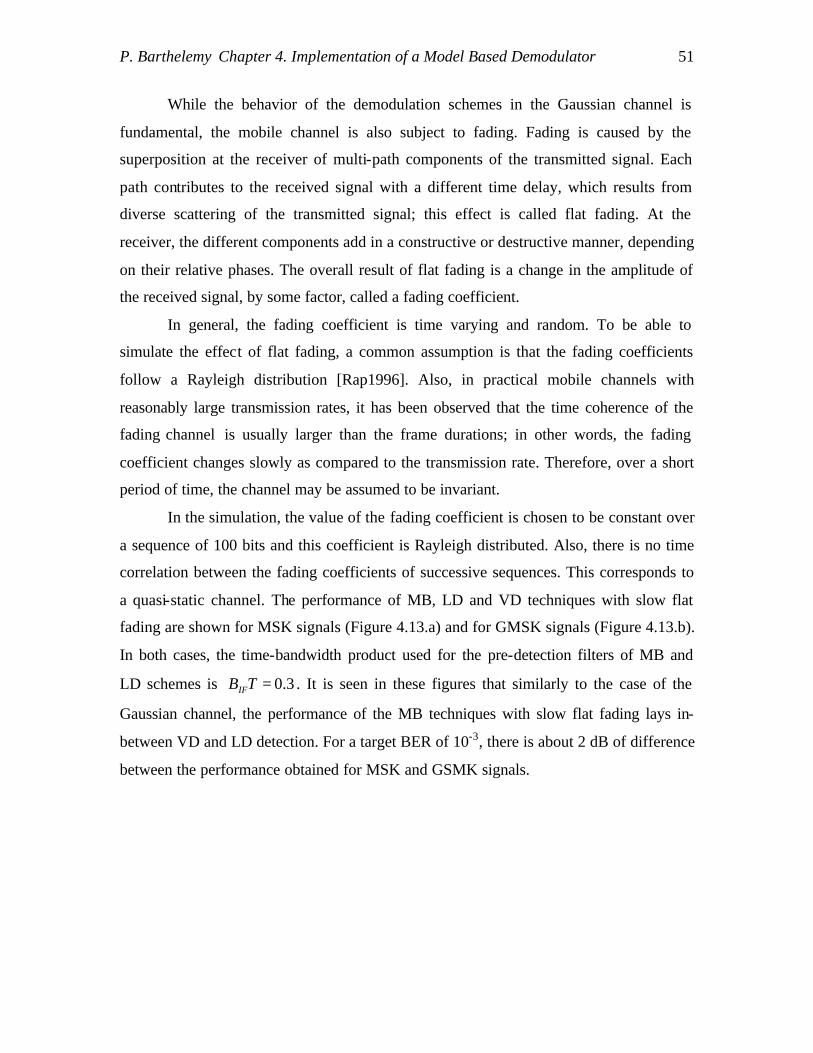
P. Barthelemy Chapter 4. Implementation of a Model Based Demodulator 51
While the behavior of the demodulation schemes in the Gaussian channel is
fundamental, the mobile channel is also subject to fading. Fading is caused by the
superposition at the receiver of multi-path components of the transmitted signal. Each
path contributes to the received signal with a different time delay, which results from
diverse scattering of the transmitted signal; this effect is called flat fading. At the
receiver, the different components add in a constructive or destructive manner, depending
on their relative phases. The overall result of flat fading is a change in the amplitude of
the received signal, by some factor, called a fading coefficient.
In general, the fading coefficient is time varying and random. To be able to
simulate the effect of flat fading, a common assumption is that the fading coefficients
follow a Rayleigh distribution [Rap1996]. Also, in practical mobile channels with
reasonably large transmission rates, it has been observed that the time coherence of the
fading channel is usually larger than the frame durations; in other words, the fading
coefficient changes slowly as compared to the transmission rate. Therefore, over a short
period of time, the channel may be assumed to be invariant.
In the simulation, the value of the fading coefficient is chosen to be constant over
a sequence of 100 bits and this coefficient is Rayleigh distributed. Also, there is no time
correlation between the fading coefficients of successive sequences. This corresponds to
a quasi-static channel. The performance of MB, LD and VD techniques with slow flat
fading are shown for MSK signals (Figure 4.13.a) and for GMSK signals (Figure 4.13.b).
In both cases, the time-bandwidth product used for the pre-detection filters of MB and
LD schemes is 0.3IFB T = . It is seen in these figures that similarly to the case of the
Gaussian channel, the performance of the MB techniques with slow flat fading lays in-
between VD and LD detection. For a target BER of 10-3, there is about 2 dB of difference
between the performance obtained for MSK and GSMK signals.

P. Barthelemy Chapter 4. Implementation of a Model Based Demodulator 52
(a)
(b)
Figure 4.13 Performance with slow flat fading of LD, MB and VD techniques for (a)
MSK signals and (b) GMSK signals.

P. Barthelemy Chapter 4. Implementation of a Model Based Demodulator 53
4.5 Summary
In this chapter, we implemented the Kumaresan and Tufts parametric frequency
estimator for the demodulation of MSK and GMSK signals. This principal component
technique, with minor modifications, permits the detection of MSK signals with low error
rates for medium SNRs. To be able to detect the signal in poor channel conditions, the
MB demodulation is combined with pre-detection filtering and sequence estimation
(Viterbi algorithm). These two techniques respectively reduce the input noise and
mitigate inter-symbol interference. An increase in the number of frequency estimates per
bit is also shown to improve the performance of sequence estimation schemes with
model-based detection.
Finally, the performance of the model-based technique is assessed through
computer simulations in two channel conditions: with AWGN and slow flat fading. The
advanced MB scheme is shown to be superior to discriminator detection and have
performance approaching coherent detection in the Gaussian and flat fading channels.
However, the resistance of MSK demodulation techniques to co-channel interference has
not been considered yet. This resistance to CCI is of prime importance as it determines
the capacity of narrowband cellular systems and is investigated in Chapter 5.

54
Chapter 5 Interference Rejection Capability of Model-Based Demodulation
A model-based demodulator for MSK and GMSK signals has been described in
Chapter 4, and the simulation results for this demodulator were obtained for the AWGN
and slow flat fading channels. The interference rejection capability of the base-station
receiver is a major concern in mobile systems. The model-based demodulator is now
assessed in the presence of co-channel interference (the only modulation format
considered is MSK) and its performance is compared to some other demodulation
schemes. In addition, demodulator diversity is introduced as a way to improve the CCI
rejection capability of individual receivers, and a combined scheme is proposed for
demodulation of MSK in CCI limited environments.
5.1 Performance of Standard Techniques with CCI
The capacity of a cellular system in a noise- limited environment can be increased
by reducing the size of the cells until the interference between the co-channel users (CCI)
of adjacent cells becomes the dominant impairment. Therefore, the ability of the base-
station receivers to reject CCI will determine the minimum size for the cells and greatly
impact on the overall system capacity.
The closed-form analysis of co-channel interference is not easy, since the
probability distribution of the interfering signals is complex. In [Chi1996] the
performance of GSMK and BPSK in presence of co-channel interference is considered.
Whereas a closed-form expression is derived for BPSK, results for GMSK are obtained
by simulation only. In some cases the effect of CCI may be modeled as AWGN. For
instance, the distribution of a single co-channel interferer in a generic angular modulation
system is shown in [Cho1999] to be Gaussian in slow Rayleigh fading. The Central Limit
Theorem implies that the sum of several CCI (with independent fading) and thermal
noise, all of these processes having Gaussian distribution, will be Gaussian. Therefore,
with the appropriate correspondence between CCI and the equivalent amount of Gaussian
noise, performance of CPM schemes with CCI and slow Rayleigh fading can be

P. Barthelemy Chapter 5. Interference Rejection Capability of MB Demodulation 55
approximated by the results in AWGN.
However, in general, the Gaussian hypothesis is only applicable when the number
of interferers is very large. When only a few interferers are present, the performance may
significantly differ from the Gaussian approximation. In [Chi1996] the Gaussian
approximation is seen to overestimate the bit error rate for BPSK and GMSK signals with
CCI. Also, in a small-cell cellular environment, co-channel interference is likely to
originate from a few signals. Adaptive antenna techniques as well as smart channel
assignment both contribute to reduce the number of co-channel interferers [Chi1996]. For
these reasons, the robustness of these demodulation techniques for a single CCI is
primarily investigated in this chapter.
The performance of the conventional demodulator for GMSK in presence of co-
channel interference has been simulated in [Yao1996], [Ada1990], [Lop1991]. In
[Yao1996] different implementations of the differential detector are compared. It is seen
that decision feedback equalization helps mitigate the interference. A 2-bit differential
detector (DD) with 2-bit decision feedback (DF) outperforms 1-bit and 2-bit DD without
DFE and 2-bit DD with 1-bit DF. Limiter-discriminator schemes are considered in
[Ada1990] with various post-detection techniques. The MLSE post-detection scheme
offers superior performance than DFE in a co-channel interference-limited environment.
Simulations results in [Ada1990] are double-checked with field experiment. Finally, a
comparison of non-coherent and coherent demodulation for GMSK in CCI is performed
in [Lop1991]. While coherent and non-coherent schemes offer very different results in
AWGN, limiter-discriminator and coherent detection have closer performance to a single
CCI [Lop1991]. In section 5.4 the performance of the model-based demodulator for MSK
and GMSK demodulation in presence of CCI is compared via computer simulations to
some of these standard techniques.
5.2 Co-channel Interference Rejection Techniques for MSK Signals
Various co-channel interference rejection techniques are possible in narrowband
systems; such as time division multiple access and frequency hoping (which is also
narrowband over short periods of time). In this section some multiuser detection and
interference cancellation techniques are overviewed. Some other methods for CCI

P. Barthelemy Chapter 5. Interference Rejection Capability of MB Demodulation 56
rejection are presented in [Las1997b]. The multiuser detection and interference
cancellation techniques have been intensively studied in the context of code division
multiple access [Ver1998]. But the extension of the multiuser detection techniques to the
narrowband GMSK signals is not straightforward, as GMSK modulation is non-linear
and non-antipodal. Moreover, depending on the phase and misalignment of the signals,
the matched filters for the co-channel users may have a very similar form, which makes
two equal power GMSK signals difficult to separate.
The optimum demodulator for the co-channel signals is the joint maximum
sequence estimation technique (JMLSE). For a single user and pulse duration of LT, the
optimum Viterbi detector for a unique MSK signals has 2L+1 states. In presence of a co-
channel user, each state of the first user can be matched with one of the 2L+1 state for the
second user. As a result the optimum detector has (2L+1)2 states [Mur1995]; in [Ran1995]
a JMLSE receiver employing a 256 states trellis is simulated. The resulting complexity
makes the use of optimum joint detection impractical.
As seen in chapter 2, the MSK format can be represented as a special case of
OQPSK with sinusoidal pulse shaping. It is shown in [Lau1986] that GMSK signals can
also be represented as a finite sum of pulse amplitude modulated (PAM) signals; this is
called the Laurent representation. Based on this representation new receivers have been
developed for GMSK signals. Approximation of GMSK signals with the principal
components of the Laurent decomposition has lead to reduced complexity single-user
receivers. Also, in [Mur1996], this representation has been employed to build optimum
and sub-optimum joint detectors. Finally, the PAM representation by Laurent facilitates
the analytical analysis of GMSK.
The optimum joint detectors for MSK-type signals employ the Viterbi algorithm
with large trellises. Alternatively, the sub-optimum decision driven multiuser detectors
can offer good resistance to co-channel interference with reduced complexity [Ver1998].
Among the decision-driven detectors, successive interference cancellation has been
investigated in [Ars2000] and [Ars2001] for narrowband signals. The output of the
single-user receiver is used to reconstruct the strong signal; this reconstructed signal is
then subtracted to the observed signal and the demodulation of the difference gives an
estimate for the weak signal. Therefore, successive interference cancellation permits the

P. Barthelemy Chapter 5. Interference Rejection Capability of MB Demodulation 57
demodulation of the weak signal. Also, by reconstructing and subtracting the weak signal
to the original signal, the estimate of the strong signal may be improved.
Another joint detector for FM signals is presented in [Ham2000]. For a complex
signal composed of two constant envelop sinusoids with known amplitudes, the
instantaneous phase of each sinusoids (two unknowns) may be calculated from the real
and imaginary parts of the sum. However, there is an ambiguity in the calculation and
two sets of phases are possible at each instant, one of which corresponding to the true
values. The algorithm proposed in [Ham2000] tracks the possible phases and selects the
values that minimize the instantaneous frequency. This approach can be applied to
demodulate CPFSK signals. However, as the effect of noise is neglected in this
technique, this non-coherent joint detector has good performance for high SNR only.
For successive interference cancellation and for other joint detection techniques as
well, an accurate estimation of the amplitude and phase for all co-channel users is
required. The estimation of these parameters necessitates complex channel estimation
processes, employing per survivor processing (PSP) for example, and introduces
additional losses.
5.3 Simulation Results of the MB Demodulator in CCI limited Environment
5.3.1 Degradation of the Performance in Presence of CCI
In this section, the performance of the model-based demodulators is simulated in
presence of co-channel interference. The co-channel interferers are either synchronous to
the signal of interest (the bit periods of the SOI and SNOI are time-aligned at the
receiver) or asynchronous. In presence of M equal-power interferers, the signal to
interference ratio (SIR) is defined as Eb,S / (M× Eb,I), and expressed in decibel. For M=1
the SIR is simply the ratio of the signal power, Eb,S, to the interferer power, Eb,I. Also, the
signal to noise ratio is measured relatively to the signal of interest.
First, the performance of four model-based schemes among the one proposed in
section 4.3.c is simulated in presence of a unique asynchronous interferer. These
techniques respectively employ symbol- level detection with 1 EPB, symbol- level
detection with 8 EPB, sequence estimation with 1 EPB, and sequence estimation with 8
EPB and were referred to as methods 2, 3, 4 and 5 in section 4.3.c.
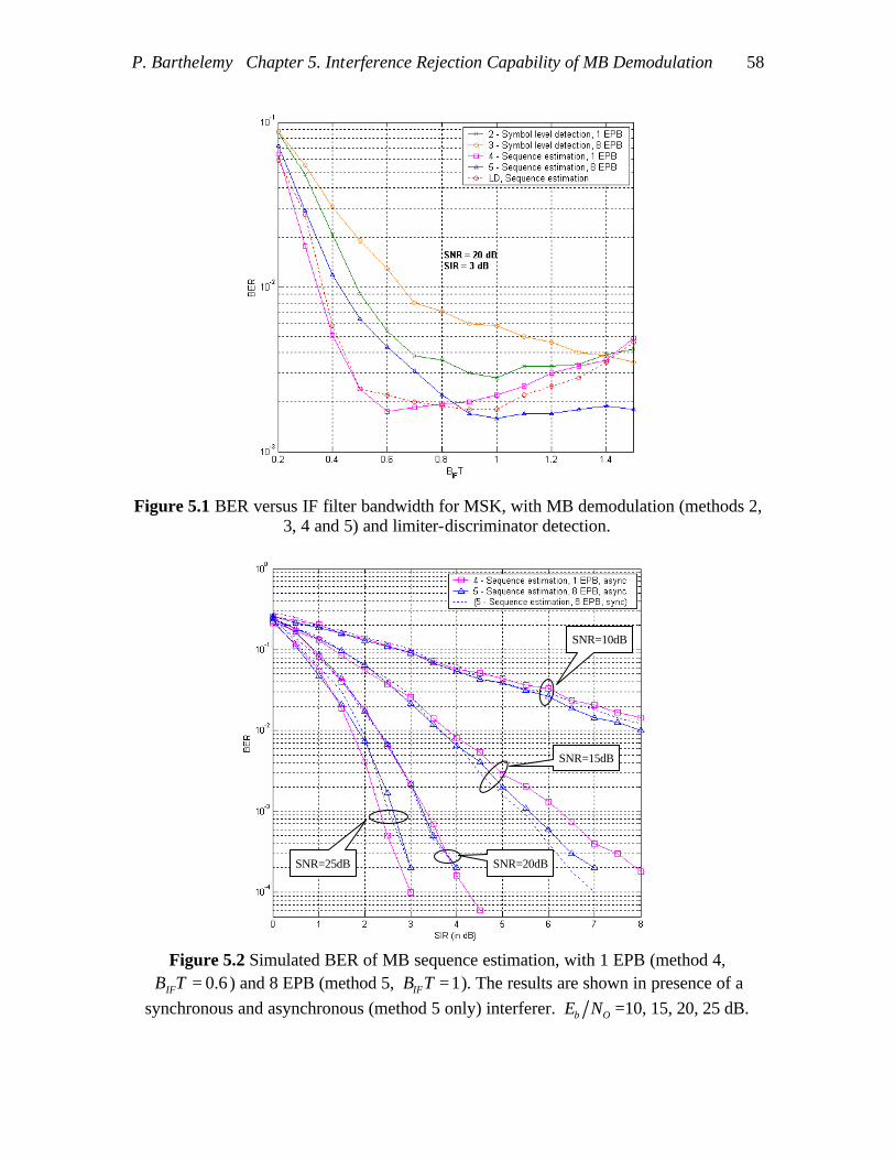
P. Barthelemy Chapter 5. Interference Rejection Capability of MB Demodulation 58
Figure 5.1 BER versus IF filter bandwidth for MSK, with MB demodulation (methods 2,
3, 4 and 5) and limiter-discriminator detection.
Figure 5.2 Simulated BER of MB sequence estimation, with 1 EPB (method 4,
0.6IFB T = ) and 8 EPB (method 5, 1IFB T = ). The results are shown in presence of a synchronous and asynchronous (method 5 only) interferer. b OE N =10, 15, 20, 25 dB.
SNR=25dB SNR=20dB
SNR=15dB
SNR=10dB

P. Barthelemy Chapter 5. Interference Rejection Capability of MB Demodulation 59
The BER is seen Figure 5.1 as a function of the IF filter bandwidth, IFB T , with a
SNR of 20dB and a SIR equal to 3dB. The simulation results obtained for the sequence
estimation scheme with discriminator detection are shown as well. It is seen that, in the
Gaussian channel, the choice of the IF filter greatly impacts the overall performance of
the demodulation. Similarly, in presence of CCI, different values for the IF filter leads to
different performance. Method 4 achieves his minimum error rate for 0.6IFB T = ,
whereas 1IFB T = is the optimum value for method 5. Regardless of this dependence on
IFB T , the performance for the MB sequence estimation schemes (4,5) is superior to that
for the MB symbol- level detection (2,3).
The error probabilities of the two model-based sequence estimation schemes are
compared as functions of the SIR and with b OE N =10, 15, 20, 25 dB (Figure 5.2). The
time-bandwidth products for method 4 and method 5 are respectively chosen to be 0.6
and 1, which are seen Figure 5.1 to be the optimum values for these techniques (at
SNR=20dB and SIR=3dB). The difference in performance for the two schemes in these
various CCI conditions is less than 0.5 dB for most cases. Due to its better resistance to
noise, method 5 has slightly superior performance for low SNR, whereas the other
technique (method 4) employing 1 EPB is more robust to CCI when the SNR is large.
Although the complexity of method 4 is significantly less than method 5, the MB results
presented later in this chapter are derived for method 5 exclusively. Also, as observed in
Figure 5.2, the BER for method 5 when the interfering user is synchronous is close to the
asynchronous case.
The effect of multiple interfering signals is now investigated. The number of
interferers is 1, 2, 3, 10, M = ∞ ; the interferers are all asynchronous and equal-power.
Thus, for a fixed SIR, the power of each interferer depends on M, such that the total
interference power is constant. For an infinite number of interferers, the Gaussian
approximation applies (central limit theorem); the effect of AWGN and CCI is simulated
as a unique Gaussian process having power equal to the sum of the noise power and the
total interference power. The simulated BER probability of method 5 in presence of
multiple interferers is reported Figure 5.3. The signal to interference ratio is equal to 6
and 10 dB.

P. Barthelemy Chapter 5. Interference Rejection Capability of MB Demodulation 60
Figure 5.3 Bit-error probability versus SNR for MSK with MB demodulation and
1,2,3,10,M = ∞ interferers and SIR=6,10dB
Figure 5.4 Performance comparison of LD, MB and VD techniques with one interferer;
SIR=1,3,6,10dB
SIR=6dB
SIR=10dB

P. Barthelemy Chapter 5. Interference Rejection Capability of MB Demodulation 61
As obvious from Figure 5.3, there is a large difference between the single and
multiple interferer cases. With the increasing number of interferers, the performance of
the MB demodulator decreases until the special case of M = ∞ , where the distribution of
the interferers becomes Gaussian. These results confirm the fact that the Gaussian
approximation ( M = ∞ ) is only valid for a large number of interferers [Chi1996].
5.3.2 Performance Comparison of LD, VD and MB Demodulation
From Figure 5.2, the optimum value for the time-bandwidth product before
discriminator detection with sequence estimation is 1IFB T = , similarly to the model-
based method 5. The results for MB (method 5, 1IFB T = ), LD ( 1IFB T = ) and VD
demodulation techniques are plotted Figure 5.4, in presence of a unique asynchronous
interferer and with SIR=1,3,6,10dB. Again, the coherent Viterbi detection outperforms
the two other schemes (as in the AWGN case). Also, the MB demodulator ranks first
among the two non-coherent sequence estimation techniques. For a targeted BER of 10-3,
and with SIR=6dB, there are 2dB of difference between the required SNR of the MB and
Viterbi detectors and an additional 2dB of difference between the MB and LD
techniques. All three techniques have limited performance for low SIR even for large
values of the SNR; and for negative SIR (the SOI is the weak signal), the SNOI would be
demodulated instead of the SOI.
The distinction of the SOI and SNOI is only possible if there exist some
difference between the signals. There are four parameters that differentiate two MSK co-
channel interferers: the phase, the delay, the instantaneous frequency and the amplitude.
For the non-coherent frequency estimation techniques such as the MB or LD
demodulators, the signals are mainly distinguished based on their instantaneous
frequency and amplitude (the strong user is demodulated). However, when the interfering
signals have almost equal power, the estimation of the frequency of the received signal is
not sufficient to distinguish the two users, since two strictly co-channel signals may have
identical instantaneous frequencies, depending on their transmitted bits. The presence of
a shift between the carrier frequencies of the two users could help in differentiating the
signals.

P. Barthelemy Chapter 5. Interference Rejection Capability of MB Demodulation 62
5.3.3 Effect of a Doppler Frequency Offset
The shift of the carrier frequency of the received signal resulting from the relative
displacement of the transmitter and the receiver is well known as the Doppler effect. For
a relative velocity of dν between the two elements, the frequency shift of the carrier is:
d df ν λ= , (5.1)
with λ denoting the wavelength of the signal. In cellular systems, the base station has a
fixed position whereas the handset may move at speed as high as a car on a highway. For
a wavelength of the order of the GHz, the maximum Doppler shift is typically around
100Hz (corresponding to a carrier frequency of 900MHz and a relative speed of 75 mph).
In the airborne scenario however, the base-station may be a high-speed aircraft and the
resulting Doppler frequency can be of the order of 500Hz (with the same frequency band
this corresponds to a relative speed of around -1160 m.s or 310 knots). Whereas the
Doppler spread of the signal limits the transmission rates of conventional receivers, it
also introduces some dissimilarity between the co-channel users, which may be exploited
to recognize the user of interest.
The parametric frequency estimators are able to correctly separate distinct
sinusoids with frequencies as close as (2 ) 2Sf N R= [Wel1996], where Sf is the
sampling rate and R is the bit rate. Also, MSK tones have frequency equal to 4df R= ± .
Therefore, two MSK signals with carrier frequencies respectively equal to 1cf and 2cf
cannot be completely separated unless 2 1-c cf f R> . When the difference between the
carriers is greater, the parametric spectral estimator outputs two distinct poles for the two
signals, while when the difference is less there may be only one pole representing the two
signals.
Figure 5.5 Relative positions of the frequency tones for two MSK signals with carrier
frequencies 1cf and 2cf : three alternative scenarios.
2cf 2cf 2cf 1cf
1cf
1cf
2 1- 4c cf f R< 2 14 - 2c cR f f R< < 2 1/ 2 -c cR f f<

P. Barthelemy Chapter 5. Interference Rejection Capability of MB Demodulation 63
However, a user with carrier frequency spaced by more than R from the signal of
interest is unlikely to be a co-channel user. For two co-channel signals, the carrier
frequencies at the transmitter are identical. The received signals however may have
different frequencies due to different Doppler shifts but this frequency deviation is
limited. For a bit rate of 10R = kbps for instance, and if the difference in frequency of the
two carriers, due to the Doppler effect, is 1kHz, then, 2 1- 10c cf f R= . Such a large
Doppler spread is unlikely to happen and is still less than the minimum frequency
difference required for the parametric estimator to output two distinct poles for the SOI
and the SNOI.
The bit error rates of the model-based technique, the discriminator and the Viterbi
detector are evaluated in presence of one SNOI having frequency slightly offset from the
frequency of the SOI (Figure 5.6). The frequency difference 2 1-c cf f ranges from 0 to
R/2, the SNR is 20 dB, and the SIR is 3dB. For the MB and LD detections, the simulation
results are shown for an IF time-bandwidth product of 1IFBT = . Also, the exact
frequency of the signal of interest is assumed to be known by the receiver.
According to this figure, not only does a frequency shift of the interferer not help
the detection of the SOI, but it even degrades the performance. The BER increases with
the increase in the frequency shift, until 2 1- / 4c cf f R= . For the large frequency shifts
the performance is improved, since the predetection filter attenuates the interference.
Also, as anticipated from Figure 5.4, the LD and MB techniques have similar
performance for 2 1- 0c cf f = . However, with the increasing difference between the
carrier frequencies, the performance of the MB technique becomes superior to that of the
discriminator. Although the range of frequency differences considered in Figure 5.6 may
not be typical for a Doppler shift, this result suggests that the robustness of MB detection
to random FM interference is improved as compared to LD technique.

P. Barthelemy Chapter 5. Interference Rejection Capability of MB Demodulation 64
Figure 5.6 BER versus frequency offset of the interferer for LD, MB and VD
demodulation techniques, SNR=20dB, SIR=1,2,3dB
SIR=1dB
SIR=2dB
SIR=3dB SNR=20dB

P. Barthelemy Chapter 5. Interference Rejection Capability of MB Demodulation 65
5.4 Demodulator Diversity: a Combined MB / VD Scheme
5.4.1 Demodulator Diversity
There does not exist a single best demodulation scheme for GMSK: for each
channel a different demodulators may be optimum. For that reason, one has to carefully
estimate the wireless channel of interest before selecting an appropriate demodulation
scheme. Rather than choosing a single technique, which may not be the best in all
scenarios, attempts have been made to use several techniques at the same time and use
this demodulation diversity to obtain the best possible performance. For instance, a smart
receiver employing a bank of K demodulators could select the output of a given
demodulator depending on the channel (demodula tor 1 for AWGN channel, demodulator
2 in CCI limited environment, demodulator 3 in slow fading…). However, due to the
possible superposition of all these effects a simple selection of one demodulation
technique is not satisfactory. Instead, the soft-output of the K demodulators can be
weighted and added together as shown on Figure 5.7 (the signals r1,r2,…,rK are identically
equal to the received signal).
Figure 5.7 Block diagram of a post detection combiner
Such post-detection combiners have been developed in the case of antenna
diversity. To combat fading, a receiver may comprise several antennas, with large
spacing to limit the correlation of the fading profiles at each antenna. The set of the K
signals r1,r2,…,rK (received from the different antennas) may be co-phased and added
before detection, but this pre-detection combining requires the tracking of the signal
Demodulator 1
X
X
X
Σ
Demodulator 2
Demodulator K
Binary Decision
wK
w2
w1 r1(t)
r2(t)
rK(t)
P. Barthelemy Chapter 5. Interference Rejection Capability of MB Demodulation 66
phase for each antenna. Post-detection combining, on the other hand, may be used with
non-coherent detection [Ada1988b]: the individual signals from each antenna are
demodulated independently and the K soft outputs are then combined before decision.
The possible methods for combining the soft outputs are equal gain combining,
maximum ratio combining and adaptive combining.
5.4.2 A Combined Demodulator for MSK
Demodulator diversity for GMSK signals is investigated in [Las1997a]. The
author chooses to combine several coherent and non-coherent demodulators. It is then
shown in this paper that the adaptive combined scheme has performance at least equal to
the best demodulator in all channel conditions and that in some cases (with CCI and
urban fading) the combined scheme may even outperform the best individual scheme. In
this part, a combined demodulation scheme for MSK signals is proposed, employing MB
and VD techniques.
The combination of the model-based and the coherent techniques to improve the
performance was suggested by the comparison of the outputs of the MB demodulator and
of the Viterbi detector. While the probability of a bit error is less for the Viterbi detection
than for the MB demodulator in the Gaussian channel and in presence of an interferer
(Figure 5.9), only a few of these bit errors are common for the two techniques. It is seen
in Figure 5.9 that the probability that the MB and VD techniques simultaneously make an
error for the same bit is much less than the probability of bit error of each individual
schemes. In other words, if there existed a genie that would be able to select the output of
the demodulator that gives the correct decision, this genie would have performance equal
to the probability of common errors (when both demodulator outputs are incorrect even
the genie is fooled). Obviously, such a genie does not exist. However, there exist some
measures for the correctness of the bit decision: one of them is the distance metric in the
trellis diagrams. As both MB and VD demodulation techniques employ a trellis to track
the signal (or its frequency as in the case of MB method), the decision metrics of the two
diagrams may be combined to improve on the individual decision. For instance, due to
the combination of noise and interference, the Viterbi detector may decide a sequence of
bits that is incorrect. This sequence has the lowest metric in the VD trellis. However, on

P. Barthelemy Chapter 5. Interference Rejection Capability of MB Demodulation 67
the MB side, the same sequence of bit may correspond to a very large metric in the MB
trellis, telling that this sequence is not correct.
The combined MB/VD demodulation scheme, which has been implemented, is
based on a coherent Viterbi detector (4 state trellis) and a model-based sequence
estimation technique with 8 frequency estimations per bit. The IF filter preceding the
model-based detection is Gaussian, has large bandwidth ( 1IFB T = ) and its time duration
is truncated to one bit. The model-based technique itself would therefore employ a 4 state
trellis for the sequence estimation process (Figure 4.11). Then a trellis is built such that
each state ( VDi ) of the VD trellis is combined with each state of the MB trellis ( MBi ).
There are a total of 4×4=16 possible states ( , )VD MBi i in the combined trellis. For a valid
transition, the decision metric from state ( , )VD MBi i to state ( , )VD MBj j is the sum of the
individual decision metrics, weighted by a factor /MB V Dµ :
( ) ( )( ) ( ) ( )/ , / , ,, ,MB V D n VD MB VD MB MB VD V D n VD VD M B n MB MBi i j j i j i jυ µ υ υ→ = × → + → , (5.1)
where the decision metrics ( ),V D n VD VDi jυ → and ( ),MB n MB MBi jυ → have been defined in
Equations 2.11 and 4.9 respectively. A valid transition is a transition
( ) ( )( ), ,VD MB VD MBi i j j→ such that both transitions ( )VD VDi j→ and ( )MB MBi j→ are
allowed and lead to an identical bit decision. The decision metric is set to infinity if the
transition is not allowed.
Figure 5.8 Block diagram of the baseband combined MB/VD demodulator
Select WL
samples MB frequency
estimation Com
bine
d V
iterb
i al
gori
thm
(1
6 st
ate
trelli
s)
Predetection filter
Select WN S
estimates
Euclidian distances
Euclidian distances
Noiseless signal paths
Noiseless MB freq. paths
r(t) ˆna

P. Barthelemy Chapter 5. Interference Rejection Capability of MB Demodulation 68
Figure 5.9 Common errors between LD and MB techniques (genie 1), and between MB
and VD techniques (genie 2) in presence of CCI and with SNR=15dB, along with the performance of the individual schemes.
Figure 5.10 BER versus /MB V Dµ for the combined MB/VD scheme with SNR=15dB and
in presence of a co-channel interferer; SIR=2dB

P. Barthelemy Chapter 5. Interference Rejection Capability of MB Demodulation 69
The factor /MB V Dµ is constant and determines the relative contribution of the VD
and MB metrics to the decision: for a large value of /MB V Dµ the performance of the
combined scheme approaches that of VD technique, whereas for small values of /MB V Dµ
the combined scheme has results similar to MB sequence estimation. The performance of
the combined scheme is shown Figure 5.10 in presence of one interferer (SIR=2dB) and
AWGN (SNR=15dB) as a function of /MB V Dµ . As previously explained, for extreme
values of the weighting factor, the results for the combined scheme approach those for
the individual techniques. However, the BER curve has a minimum between these two
extreme scenarios, corresponding to the optimum combination of the decision metrics.
The optimum value for /MB V Dµ depends on the SIR and SNR. When employing maximum
ratio combining (MRC) the weights of the decision metrics before combining should be
updated for each value of the SIR and SNR. However for simplicity, /MB V Dµ is fixed to its
optimum value at SIR=2dB and SNR=15dB (corresponding to the minimum BER of
Figure 5.10); resulting in a small degradation of the performance.
Before presenting the results for the MB/VD schemes, it may be noted from
Figure 5.9 that the number of common errors between LD and MB sequence estimation
techniques is large. As this probability of common error is a lower bound for the
performance of the combined scheme, it has not been tried to implement this combined
MB/LD scheme.
The simulation results for the combined MB/VD scheme are shown Figure 5.11
and Figure 5.12. For comparison, the results of the VD and MB demodulators are also
reported on these figures. Figure 5.11 presents the result of the combined scheme in
AWGN. The MB branch of the combined technique utilizes an IF filter with 1IFB T = .
For this value of the time-bandwidth product, the performance of MB technique itself is
inferior to VD by more than 2dB. The combined scheme however has performance
approaching Viterbi detection (there is less than 0.5dB of degradation). The superiority of
the VD technique to the MB/VD is expected since the coherent Viterbi detection is the
MLSE (optimum) in AWGN. Moreover, the weighting coefficient chosen for MB/VD is
optimized for a CCI scenario; the best value for /MB V Dµ in AWGN would be /MB VDµ = ∞ ,
such that the MB/VD results match the MLSE performance.

P. Barthelemy Chapter 5. Interference Rejection Capability of MB Demodulation 70
Figure 5.11 Simulated BER versus /b OE N for the MB ( 1IFB T = and 0.3IFB T = ), VD
and combined MB/VD techniques
Figure 5.12 Performance of the combined MB/VD scheme in presence of CCI and with
SNR=15 and 20 dB along with the results for the MB, VD and genie approaches.
SNR=20dB
SNR=15dB
P. Barthelemy Chapter 5. Interference Rejection Capability of MB Demodulation 71
In AWGN the VD technique cannot is superior to any other demodulation
scheme. But, in presence of CCI the coherent detector has sub-optimum performance,
and therefore a demodulation scheme employing diversity combining may give an
improved result as compared to the simple Viterbi detector. Actually, it is seen in Figure
5.12 that the MB/VD demodulator is superior to the VD technique in presence of an
asynchronous interferer and with SNR=15 and 20dB. The difference in performance at
BER=10-3 between the VD and MB/VD schemes is 0.25dB when SNR=15dB and more
than 0.5dB when SNR=20dB (in terms of minimum SIR required to achieve the target
BER). In determining the dependence of the overall capacity of narrowband systems to
the robustness of the receiver to CCI, this small difference may be significant.
Also, a combined MB/VD scheme could be of interest as the first stage of an SIC
receiver. Due to the error propagation problem in successive interference cancellation,
the performance of the first stage (demodulation of the strong signal) acts as a bottleneck
for the following stages of SIC. For two co-channel signals, it has been observed that the
probability of bit error for the demodulation of the weak user is similar to the BER for the
strong user when the SNR is large. Therefore, a SIC receiver employing the combined
MB/VD receiver to demodulate the strong signal (and a simpler receiver at the second
stage) could achieve good performance when the difference in power of the two signals is
as low as 2dB and the SNR=20dB.
5.5 Summary of the Simulation Results
5.5.1 Advantages of MB Demodulation
The model-based sequence estimation scheme proposed in Chapter 4 has been
simulated for MSK signals with co-channel interference. The performance was shown for
different SNR and SIR in the case of a single and multiple CCI, the interferers were
either synchronous or asynchronous, and the possible shift of the carrier frequency of the
interferer was investigated. The simulation results of the MB technique with CCI are
slightly superior to the limiter-discriminator, but the coherent receiver outperforms the
MB scheme. An improved MB/VD receiver, which exploits demodulation diversity, is
presented, with performance surpassing the other simulated schemes.

P. Barthelemy Chapter 5. Interference Rejection Capability of MB Demodulation 72
5.5.2 Complexity of the MB Techniques
The performance comparison of the model-based demodulation with the standard
non-coherent receivers, and the comparison of the combined scheme with the
conventional coherent receivers have shown the possible benefits of MB techniques.
However, the computational complexity of such techniques should not be ignored.
To obtain the model parameters, the principal component technique employs a
singular value decomposition (SVD) of the data matrix X. This matrix has dimension
2( )N p p− × for the modified covariance method. For a 1 2M M× matrix, with 1 2M M≤
the SVD has a computational complexity of 21 2( )O M M (the number of additions and
multiplications are proportional to 21 2M M ) [Gol1989]. Therefore, the complexity of the
SVD for the data matrix X is 2({2( )} )O N p p− when 2 3p N≥ . Then the extraction of
the frequency from the estimated parameters requires either the evaluation of the
frequency response of the parametric filter for K frequencies which has complexity
O(pK), or rooting of the polynomial which is O(p3). Those operations are necessary for
each frequency estimate. When the number of estimate is greater than the number of bits
( WS N< ), the complexity of the detection is multiplied by WN S .
Finally, tracking the frequency using the Viterbi algorithm necessitates further
computations: for a trellis of 2L+1 states, which is employed in the MB sequence
estimation process for a channel of order L-1 and multiple estimates per bits, the
computational complexity is O(2L+2) [Ver1998]. The computational complexity of the
limiter-discriminator with Viterbi equalization and of the coherent Viterbi receiver are
principally attributable to the Viterbi algorithm employed in these techniques. On the
contrary, for reasonably small trellises, the complexity of the parametric frequency
estimation dominates the overall complexity of the MB demodulation.

73
Chapter 6 Conclusions and Future Work
6.1 Conclusions
In this thesis, parametric frequency estimation and its application to demodulation
of CPM in presence of CCI were investigated. In the first part of the thesis (Chapter 2 and
Chapter 3), MSK modulation format and parametric frequency estimation were
overviewed. In Chapter 2, we detailed the properties of MSK and GMSK signals and the
most common demodulation schemes available for these modulation formats. In Chapter
3 we described the modified covariance and the principal component methods to estimate
the parameters of the autoregressive model and presented two techniques to extract the
frequency from these parameters.
In the second part (Chapters 4 and 5), various demodulators for MSK, employing
parametric frequency estimation were proposed. The performance of these schemes was
assessed via computer simulations and compared to some of the conventional
demodulation techniques. In Chapter 4, a model-based demodulator employing sequence
estimation was implemented. For MSK and GMSK signals, in AWGN and flat fading,
this technique outperforms discriminator detection and approaches the performance of
coherent detection. The behavior of these diverse techniques in presence of interference
was investigated in Chapter 5. Additionally, demodulator diversity was proposed as a
way to improve the performance of the individual schemes. It was seen that, with CCI, a
technique combining model-based and Viterbi detection is superior to the simple
coherent Viterbi detector.
The implementation of a non-coherent model-based sequence estimator for MSK
signals and the study of demodulation diversity combined with model-based approach,
are the two main contributions of this thesis. These proposed model-based receivers have
good CCI rejection capabilities, which make them attractive for applications in which
CCI is very problematic like the airborne scenario.
The limitations to the model-based approach were also investigated in Chapter 5.
In particular, the computational complexity is a major drawback of parametric frequency
P. Barthelemy Chapter 6. Conclusions and Future Work 74
estimation. Also, autoregressive modeling techniques assume that the signal is stationary
over the period of observation. This assumption is not correct in presence of non-
synchronous interference, and is also inexact for distorted MSK signals (distorted by the
premodulation and predetection filters). Moreover, the frequency separation between the
user of interest and the interferers may be lower than the resolution of the parametric
frequency estimator, which limits the performance of the MB receiver.
6.2 Suggestions for Future Work
The simulation results in presence of CCI were principally derived for the 8 EPB
model-based technique and MSK signals. In this technique the receiver performs eight
frequency estimations per bit (EPB) utilizing the Kumaresan and Tufts estimator after
filtering, and tracks this instantaneous frequency with the Viterbi algorithm. The
complexity of this technique has been discussed in Chapter 5 and is a major limitation to
its implementation. Various techniques have been proposed in Chapter 4 to reduce the
complexity of the MB demodulator (single estimation per bit; partial frequency response
instead of the polynomial rooting). Further simulation is needed to evaluate the
degradation of performance of the reduced complexity demodulator in presence of CCI.
Also, a combined technique employing a coherent detector and low complexity MB
detection could be implemented. The results of these diverse methods with CCI may be
derived for MSK and GMSK signals.
The combined scheme proposed in Chapter 5 employs the model-based and the
coherent detectors and jointly tracks the soft outputs of these two demodulation schemes.
The performance improvement obtained by demodulation diversity is caused by the
dissimilarity of the two techniques and their different behaviors in presence of CCI (low
probability of common errors). Although a combined scheme employing the coherent
technique and a conventional non-coherent technique, like the limiter-discriminator, may
not provide as much improvement, it has been shown in [Las1997a] that this technique
could still outperform the coherent detector. In [Las1997a] however, the use of sequence
estimation with demodulation diversity combining has not been considered; a combined
scheme employing the conventional coherent and non-coherent detectors and sequence
estimation would have reasonable complexity and may achieve good performance.
P. Barthelemy Chapter 6. Conclusions and Future Work 75
There does not exist a perfect solution to the problem of co-channel interference
rejection for MSK signals. The complexity of the optimum joint detection is prohibitive
but sub-optimum techniques are unable to properly separate nearly equal-power users. It
may also be questioned whether the complexity of the non-coherent MB technique is
preferable to the phase synchronization process required for the coherent schemes.
Finally, new demodulators for GMSK have recently been created based on Laurent
decomposition. The representation of GMSK signal as a sum of PAM signal is promising
as it permits the implementation of conventional multiuser detection techniques with
acceptable complexity.

P. Barthelemy Chapter 6. Conclusions and Future Work 76

77
Bibliography [Ada1988a] F. Adachi, K. Ohno, “Performance Analysis of GMSK Frequency Detection
with Decision Feedback Equalization in Digital Land Mobile Radio”, Proceedings of the IEEE, vol. 135, no. 3, pp. 199-207, June 1988
[Ada1988b] F. Adachi, K. Ohno, “Experiments on Postdetection Diversity for narrowband Digital FM Mobile Radio”, Electronics Letters, vol. 24, no. 24, pp. 1491-1493, November 1988
[Ada1990] F. Adachi , K. Ohno, “Performance Evaluation of Various Decision Schemes
for Frequency Demodulation of Narrow-Band Digital FM Signals in Land Mobile Radio”, IEEE Transactions on Vehicular Technology, vol. 39, no. 2, pp. 109-116, May 1990
[And1986] J. B. Anderson, T. Aulin, C. E. Sundberg, Digital Phase Modulation, Plenum
Press, New York, NY, 1986 [Ars2000] H. Arslan, K. Molnar, “Iterative Cochannel Interference Cancellation in
Narrowband Mobile Radio Systems”, IEEE Emerging Technology Symposium on Broadband, Wireless Internet Access, April 2000
[Ars2001] H. Arslan, K. Molnar, “Cochannel Interference Suppression with Successive
Cancellation in Narrow-Band Systems”, IEEE Communications Letters, vol. 5, no. 2, pp. 37-39, February 2001
[Bay2000] S. Bayram, Overloaded Array Processing: System Analysis, Signal Extraction
Techniques, and Time-Delay Estimation, Master Thesis, Virginia Polytechnic Institute and State University, December 2000
[Ben1999] S. Benedetto, E. Biglieri, Principles of Digital Transmission With Wireless
Applications, Kluwer Academic / Plenum Publishers, New York, NY, 1999 [Boa1992a] B. Boashash, “Estimating and Interpreting the Instantaneous Frequency of a
Signal - Part 1: Algorithms and Applications”, Proceedings of the IEEE, vol. 80, no. 4, pp. 520-538, April 1992
[Boa1992b] B. Boashash, “Estimating and Interpreting the Instantaneous Frequency of a
Signal - Part 2: Algorithms and Applications”, Proceedings of the IEEE, vol. 80, no. 4, pp. 540-568, April 1992
[Chi1996] M. Chiani, “Performance of BPSK and GMSK with Multiple Cochannel
Interferers”, 7th IEEE International Symposium on Personal, Indoor and Mobile Radio Communications, pp. 833-837, October 1996
78
[Cho1999] J. Chow, N.C. Beaulieu, “Analysis of Cochannel Interference in Angle
Modulation Systems”, IEEE Pacific Rim Conference on Communications, Computers and Signal Processing, pp. 123-127, August 1999
[Chu1984] K. S. Chung, “Generalized Tamed Frequency Modulation and its Application
for Mobile Radio Communications”, IEEE Journal on Selected Areas in Communications, vol. SAC-2, pp. 487-497, July 1984
[Clar1993] P. M. Clarkson, Optimal and Adaptive Signal Processing, CRC Press, Boca
Raton, Fl, 1993 [Cou2001] L. W. Couch, Digital and Analog Communication Systems, 6th Edition,
Prentice Hall, Upper Saddle River, NJ, 2001 [Gol1989] G. H. Golub, C. F. Van Loan, Matrix Computations Second Edition, The
Johns Hopkins University Press, Baltimore, Ma, 1989 [Ham2000] J. Hamkins, “An Analytic Technique to Separate Cochannel FM Signals”,
IEEE Transactions on Communications, vol. 48, no. 4, pp. 543-546, April 2000 [Hay1996] S. Haykin, Adaptive Filter Theory Third Edition, Prentice Hall, Upper Saddle
River, NJ, 1996 [Hir1984] M. Hirono, T. Miki, K. Murota, “ Multilevel Decision Method for Band-
Limited Digital FM with Limiter-Discriminator Detection”, IEEE Journal on Selected Areas in Communications, vol. SAC-2, pp. 498-506, July 1984
[Iwa1995] Y. Iwanami, “Performance of Sequence Estimation Scheme of Narrowband
Digital FM Signals with Limiter-Discriminator Detection”, IEEE Journal on Selected Areas in Communications, vol. 13, no. 2, pp. 310-315, February 1995
[Jen1991] P. M. R. Jensen, Singular Value Decomposition and its Application to
Autoregressive Parametric Spectral Estimation, Technical Report R91-33, Department of Communication Technology, Institute of Electronic Systems, Aalborg University, Denmark, August 1991
[Kay1988] S. M. Kay, Modern Spectral Estimation Theory & Application, Prentice Hall,
Upper Saddle River, NJ, 1988 [Kay1993] S. M. Kay, Fundamentals of Statistical Signal Processing Estimation Theory,
Prentice Hall, Upper Saddle River, NJ, 1993 [Kum1982a] R. Kumaresan, D. W. Tufts, “Estimating the Parameters of Exponentially
Damped Sinusoids and Pole-Zero Modeling in Noise” IEEE Transactions on
79
Acoustics, Speech and Signal Processing, vol. ASSP-30, no. 6, pp. 833-840, December 1982
[Kum1982b] R. Kumaresan, D. W. Tufts, “Estimation of Frequencies of Multiple
Sinusoids: Making Linear Prediction Perform Like Maximum Likelihood”, Proceedings of the IEEE, vol. 79, no. 9, September 1982
[Las1997a] J. D. Laster, Robust GMSK Demodulation Using Demodulator Diversity and
BER Estimation, PhD Dissertation, Virginia Polytechnic Institute and State University, Blacksburg, Va, March 1997
[Las1997b] J. D. Laster, J. H. Reed, “Interference Rejection in Digital Wireless
Communications”, IEEE Signal Processing Magazine, vol. 14, no. 3, pp. 37-62, May 1997
[Lau1986] P. A. Laurent, “Exact and Approximate Construction of Digital Phase
Modulations by Superposition of Amplitude Modulated Pulses (AMP)”, IEEE Transactions on Communications, vol. 34, no. 2, pp. 150-160, February 1986
[Lee1988] S.U. Lee, Y. M. Chung, J. M. Kim, “On the Bit Error Probabilities of GMSK
in the Rayleigh Fading Channels”, IEEE 38th Vehicular Technology Conference, pp. 249-254, June 1988
[Lop1991] L. P. Lopes “Coherent and Limiter-Discriminator Detection of GMSK in
Interference Limited Conditions”, Electronic Letters, vol. 27, no. 25, pp. 2313-2315, December 1991
[Mur1981] K. Murota, K. Hirade, “GMSK Modulation for Digital Mobile Radio
Telephony”, IEEE Transactions on Communications, vol. 29, no. 7, pp. 1044-1050, July 1981
[Mur1995] P. A. Murphy, G. E. Ford, “Cochannel Demodulation for Continuous Phase
Modulated Signals”, Proceedings of the 28th Asilomar Conference on Signals, Systems, and Computers, 1995
[Mur1996] P.A. Murphy and G.E. Ford, "Cochannel Receivers for CPM Signals Based
Upon the Laurent Representation," Proceedings Virginia Tech's 6th Symposium on Wireless Personal Communications, Blacksburg, VA, June 1996
[Pro2001] J. G. Proakis, Digital Communications Fourth Edition, McGraw-Hill, New
York, NY, 2001 [Ran1995] P. A. Ranta, A. Hottinen, Z. C. Honkasalo, “Co-Channel Interference
Canceling Receiver for TDMA Mobile Systems”, IEEE International Conference on Communications, vol. 1, 1995

80
[Rap1996] T. S. Rappaport, Wireless Communications, Prentice Hall PTR, Upper Saddle River, NJ, 1996
[Rim1988] B. E. Rimoldi, “A Decomposition Approach to CPM”, IEEE Transactions on
Information Theory, vol. 34, no. 2, pp. 260-270, March 1988 [Sim1983] M. K. Simon, C. C. Wang, “Differential Versus Limiter Discriminator
Detection of Narrowband FM”, IEEE Transactions on Communications, vol. 31, no. 11, November 1983
[Sim1984] M. K. Simon, C. C. Wang, "Two-Bit Differential Detection of MSK",
GLOBECOM '84 Conference Record, pp. 2231-2236, December 1984 [Skl1988] B. Sklar, Digital Communications Fundamentals and Applications, Prentice
Hall, Upper Saddle River, NJ, 1988 [Sto1997] P. Stoica, R. L. Moses, Introduction to Spectral Analysis, Prentice Hall, Upper
Saddle River, NJ, 1997 [Suz1981] H. Suzuki, “Optimum Gaussian Filter for Differential Detection of MSK”,
IEEE Transactions on Communications, vol. 29, no. 6, pp. 916-918, June 1981 [The1992] C. W. Therrien, Discrete Random Signals and Statistical Signal Processing,
Prentice Hall, Upper Saddle River, NJ, 1992 [Tun1994] C. C. Tung, J. N. Livingston, “Viterbi Detector for Narrow-Band Digital FM
with Limiter-Discriminator Detection”, GLOBECOM '94 Conference Record, pp. 201-205, 1994
[Vas2000] S. V. Vaseghi, Advanced Digital Signal Processing and Noise Reduction,
Second Edition, John Wiley & Sons, New York, NY, 2000 [Ver1998] S. Verdu, Multiuser Detection, Cambridge University Press, Cambridge, UK,
1998 [Wel1996] M. L. Welborn, Co-Channel Interference Rejection Using a Model-based
Demodulator, Master Thesis, Virginia Polytechnic Institute and State University, Blacksburg, Va, January 1996
[Yao1996] S. K. Yao, J. H. Reed, J. D. Laster, “GMSK Differential Detectors with
Decision Feedback in Multipath and CCI Channels”, GLOBECOM '96 Conference Record, 1996, vol. 3, pp.1830 -1834, 1996
[Yon1988] A. Yongacoglu, D. Makrakis, K. Feher, “Differential Detection of GMSK
Using Decision Feedback”, IEEE Transactions on Communications, vol. 36, no. 6, pp. 644-649, June 1988

81
Vita
Pierre Barthélemy was born on November 6, 1978, in Evry, France. He attended
Lycée Chaptal, Paris, France and transferred to the Ecole Supérieure d’Electricité
(SUPELEC), Metz, France in 1998. He received his Engineering Degree from SUPELEC
in July 2002. From August 2000 to May 2002, he attended Virginia Polytechnic Institute
and State University Graduate School. Pierre joined the Mobile and Portable Radio
Research Group (MPRG) in January 2001. He received his Master of Science Degree
from Virginia Tech in May 2002 under Dr Brian D. Woerner. His research interests
include digital signal processing, multiuser detection and modulation.
![Interactive Kalman Filtering for Differential and … · coherent demodulation of CPM and CPFSK respectively. In [15], O. Loffeld utilized the EKF in the demodulation of noisy phase](https://static.fdocuments.us/doc/165x107/5b59e1f17f8b9a88698dfa31/interactive-kalman-filtering-for-differential-and-coherent-demodulation-of-cpm.jpg)


![Optimal Demodulation of Reaction Shift Keying Signals in ... · Two components in di usion-based molecular communication system are modulation and demodulation. ... [8, 9], Pulse](https://static.fdocuments.us/doc/165x107/5ac6916d7f8b9a2b5c8e415c/optimal-demodulation-of-reaction-shift-keying-signals-in-components-in-di-usion-based.jpg)