A Methodology to Assess the Value of Integrated

Hydropower and Wind Generation

by

Mitch A. Clement

B.A., Wheaton College, 2000

B.S., University of Colorado, 2010

A thesis submitted to the

Faculty of the Graduate School of the

University of Colorado in partial fulfillment

of the requirements for the degree of

Master of Science

Department of Civil, Environmental and Architectural Engineering

2012

This thesis entitled:A Methodology to Assess the Value of Integrated Hydropower and Wind Generation

written by Mitch A. Clementhas been approved for the Department of Civil, Environmental and Architectural Engineering

Edith Zagona

Balaji Rajagopalan

JoAnn Silverstein

Date

The final copy of this thesis has been examined by the signatories, and we find that both thecontent and the form meet acceptable presentation standards of scholarly work in the above

mentioned discipline.

Clement, Mitch A. (M.S. Civil Engineering)

A Methodology to Assess the Value of Integrated Hydropower and Wind Generation

Thesis directed by Professor Edith Zagona

Installed wind generation capacity has increased at a rapid rate in recent years. Wind gen-

eration provides numerous economic, social and environmental benefits, but it also carries inherent

variability and uncertainty, which can increase the need for additional balancing reserves, genera-

tion resources that can adjust their output rapidly to keep power supply in balance with demand.

Hydropower is an inexpensive and flexible generating resource that has been considered one of the

best resources to provide the necessary balancing reserves for wind. Hydropower’s flexibility and

capacity are limited, however, by non-power constraints associated with environmental and water

management objectives that have not been fully accounted for in previous wind integration studies.

We present a methodology to evaluate hydropower and wind integration using the RiverWare river

system and hydropower modeling tool. The model represents both the physical characteristics

of the hydropower system and accounts for realistic non-power policy constraints. An economic

evaluation is provided that includes the value of both energy and ancillary services. In addition,

operational outputs include the ability to satisfy all policy constraints. The methodology is applied

to a test case integrated hydropower and wind generation system including five hydropower projects

in a run-of-river configuration for a range of wind penetration levels and hydrologic conditions.

Results show that wind at low penetrations adds economic value to the system. As the

installed capacity increases, additional wind generation has diminishing returns, primarily due to

increased reserve requirements. Increased wind capacity also causes increases the number of policy

constraint violations. Non-power constraints have a significant impact on total system value, but

that relative impact varies depending on system conditions. Complex interactions between policy

and the physical system result in a highly non-linear response of the system to changes in wind

penetration. Utilization of goal programming makes it possible to capture these effects that would

iv

be missed without a realistic representation of both the integrated physical system and its operating

policy. This methodology can be used to provide an improved representation of hydropower systems

in future wind integration studies.

v

Acknowledgements

I would like to thank my advisor, Edie Zagona, for providing this research opportunity. This

project would not have been possible without her guidance throughout the process.

Tim Magee at CADSWES provided invaluable support throughout this project both on

technical matters and in analyzing the broader implications of the work. I am grateful to benefit

from his experience and expertise. I would also like to thank my other committee members, Balaji

Rajagopalan and JoAnn Silverstein for their time and valuable input on this thesis.

I am very grateful to the Hydro Research Foundation and the Department of Energy for

providing me with a fellowship to fund this research.

Joe Taylor from Mid-Columbia Central is responsible for providing Mid-C request data used

in this research. In addition, he provided insight into Mid-C operations and policy that influenced

this work and facilitated the modeling of realistic operating conditions.

Much of the groundwork for this project was laid by a previous project sponsored by Oak

Ridge National Laboratory to model wind integration in the Mid-Columbia system. I thank Bren-

nan Smith of ORNL for his contribution and guidance through that project.

Bri-Mathias Hodge and Michael Milligan of the National Renewable Energy Laboratory pro-

vided insight on wind modeling and facilitated the acquisition of wind forecast data that made

possible the development of the wind forecast model in this research.

Finally, I would like to thank my wife, Katie, and our daughters, Anna, Josie and Ruthie,

for providing endless support, encouragement and patience throughout this process.

Contents

Chapter

1 Introduction 1

1.1 Overview . . . . . . . . . . . . . . . . . . . . . . . . . . . . . . . . . . . . . . . . . . 1

1.2 Existing Work on Hydropower and Wind Integration . . . . . . . . . . . . . . . . . . 5

1.3 Significance of this Research . . . . . . . . . . . . . . . . . . . . . . . . . . . . . . . . 10

2 Modeling and Methodology 15

2.1 Conceptual Model . . . . . . . . . . . . . . . . . . . . . . . . . . . . . . . . . . . . . 15

2.1.1 Model Overview . . . . . . . . . . . . . . . . . . . . . . . . . . . . . . . . . . 15

2.1.2 Ancillary Services . . . . . . . . . . . . . . . . . . . . . . . . . . . . . . . . . 19

2.1.3 Markets . . . . . . . . . . . . . . . . . . . . . . . . . . . . . . . . . . . . . . . 21

2.2 Run Sequence . . . . . . . . . . . . . . . . . . . . . . . . . . . . . . . . . . . . . . . . 23

2.3 Hydropower Modeling in RiverWare . . . . . . . . . . . . . . . . . . . . . . . . . . . 28

2.3.1 RiverWare Optimization - Preemptive Linear Goal Programming . . . . . . . 28

2.3.2 Power Modeling . . . . . . . . . . . . . . . . . . . . . . . . . . . . . . . . . . 30

2.3.3 Ancillary Services . . . . . . . . . . . . . . . . . . . . . . . . . . . . . . . . . 30

2.3.4 Economic Modeling . . . . . . . . . . . . . . . . . . . . . . . . . . . . . . . . 34

2.3.5 Other Physical Processes . . . . . . . . . . . . . . . . . . . . . . . . . . . . . 39

2.4 Test System . . . . . . . . . . . . . . . . . . . . . . . . . . . . . . . . . . . . . . . . . 40

2.4.1 Physical System Description . . . . . . . . . . . . . . . . . . . . . . . . . . . . 40

vii

2.4.2 Policy . . . . . . . . . . . . . . . . . . . . . . . . . . . . . . . . . . . . . . . . 44

2.4.3 Input Data . . . . . . . . . . . . . . . . . . . . . . . . . . . . . . . . . . . . . 52

2.4.4 Scenario Descriptions . . . . . . . . . . . . . . . . . . . . . . . . . . . . . . . 62

2.5 Assumptions and Simplifications . . . . . . . . . . . . . . . . . . . . . . . . . . . . . 68

3 Wind Generation Modeling 70

3.1 Actual Wind Generation Data . . . . . . . . . . . . . . . . . . . . . . . . . . . . . . 71

3.2 Wind Generation Forecast . . . . . . . . . . . . . . . . . . . . . . . . . . . . . . . . . 74

3.2.1 Existing Statistical Wind Forecast Methodologies . . . . . . . . . . . . . . . . 74

3.2.2 Analysis of Observed Wind Generation Forecast Error . . . . . . . . . . . . . 75

3.2.3 Day-ahead Wind Forecast Model . . . . . . . . . . . . . . . . . . . . . . . . . 78

3.2.4 Wind Forecast Models for Two and Three Days Ahead . . . . . . . . . . . . . 83

4 Assessing the Value of Integrated Hydropower and Wind Generation 86

4.1 Introduction . . . . . . . . . . . . . . . . . . . . . . . . . . . . . . . . . . . . . . . . . 86

4.1.1 Overview . . . . . . . . . . . . . . . . . . . . . . . . . . . . . . . . . . . . . . 86

4.1.2 Existing Wind and Hydropower Integration Studies . . . . . . . . . . . . . . 87

4.1.3 Significance of this Research . . . . . . . . . . . . . . . . . . . . . . . . . . . . 88

4.2 Modeling and Methodology . . . . . . . . . . . . . . . . . . . . . . . . . . . . . . . . 89

4.2.1 Conceptual Model . . . . . . . . . . . . . . . . . . . . . . . . . . . . . . . . . 89

4.2.2 Hydropower Modeling in RiverWare . . . . . . . . . . . . . . . . . . . . . . . 90

4.2.3 Run Sequence . . . . . . . . . . . . . . . . . . . . . . . . . . . . . . . . . . . . 93

4.3 Wind Modeling . . . . . . . . . . . . . . . . . . . . . . . . . . . . . . . . . . . . . . . 94

4.3.1 Actual Wind . . . . . . . . . . . . . . . . . . . . . . . . . . . . . . . . . . . . 94

4.3.2 Wind Forecast . . . . . . . . . . . . . . . . . . . . . . . . . . . . . . . . . . . 96

4.4 Test Case . . . . . . . . . . . . . . . . . . . . . . . . . . . . . . . . . . . . . . . . . . 99

4.4.1 Physical Hydropower System . . . . . . . . . . . . . . . . . . . . . . . . . . . 99

4.4.2 Policy . . . . . . . . . . . . . . . . . . . . . . . . . . . . . . . . . . . . . . . . 99

viii

4.4.3 Scenarios . . . . . . . . . . . . . . . . . . . . . . . . . . . . . . . . . . . . . . 104

4.4.4 Input Data . . . . . . . . . . . . . . . . . . . . . . . . . . . . . . . . . . . . . 106

4.5 Discussion of Results . . . . . . . . . . . . . . . . . . . . . . . . . . . . . . . . . . . . 107

4.5.1 Impact of Non-power Policy . . . . . . . . . . . . . . . . . . . . . . . . . . . . 107

4.5.2 Isolated Effects of Wind Forecast Error, Variability and Energy . . . . . . . . 116

4.5.3 Sensitivities to System Characteristics . . . . . . . . . . . . . . . . . . . . . . 117

4.6 Conclusions . . . . . . . . . . . . . . . . . . . . . . . . . . . . . . . . . . . . . . . . . 122

5 Conclusions and Recommendations 124

5.1 Summary . . . . . . . . . . . . . . . . . . . . . . . . . . . . . . . . . . . . . . . . . . 124

5.2 Conclusions . . . . . . . . . . . . . . . . . . . . . . . . . . . . . . . . . . . . . . . . . 125

5.3 Future Work . . . . . . . . . . . . . . . . . . . . . . . . . . . . . . . . . . . . . . . . 129

Bibliography 133

Appendix

A Plant Power Tables 138

B Wind Modeling Supplemental Analysis 144

B.1 Wind Variability Analysis . . . . . . . . . . . . . . . . . . . . . . . . . . . . . . . . . 144

B.2 Wind Forecast Model Analysis . . . . . . . . . . . . . . . . . . . . . . . . . . . . . . 145

C Additional Model Results and Analysis 148

C.1 Policy Effects on System Economic Value . . . . . . . . . . . . . . . . . . . . . . . . 148

C.2 Impacts of Flow Constraints on Upstream Reservoir Operations . . . . . . . . . . . . 151

C.3 Constraint Violations . . . . . . . . . . . . . . . . . . . . . . . . . . . . . . . . . . . . 153

C.4 Effects of Wind Forecast Error, Variability and Energy . . . . . . . . . . . . . . . . . 155

C.5 Effects of Reserve Requirements . . . . . . . . . . . . . . . . . . . . . . . . . . . . . . 161

ix

C.6 Summer Scenario with Spring Prices . . . . . . . . . . . . . . . . . . . . . . . . . . . 163

C.7 Effects of Load Levels and Transmission Limits . . . . . . . . . . . . . . . . . . . . . 165

C.8 Market Depth Effects . . . . . . . . . . . . . . . . . . . . . . . . . . . . . . . . . . . 168

C.9 Effects of Wind Timing and Correlation with Prices . . . . . . . . . . . . . . . . . . 168

Tables

Table

2.1 Reservoir storage and elevation-volume parameters . . . . . . . . . . . . . . . . . . . 42

2.2 Tailwater table . . . . . . . . . . . . . . . . . . . . . . . . . . . . . . . . . . . . . . . 43

2.3 Plant power characteristics . . . . . . . . . . . . . . . . . . . . . . . . . . . . . . . . 44

2.4 Load input data for base scenarios . . . . . . . . . . . . . . . . . . . . . . . . . . . . 53

2.5 Load forecast model parameters . . . . . . . . . . . . . . . . . . . . . . . . . . . . . . 54

2.6 Incremental reserve requirments, spring base scenario . . . . . . . . . . . . . . . . . . 61

2.7 Load input data for alternative load level scenarios . . . . . . . . . . . . . . . . . . . 67

3.1 Statistics of normalized observed wind generation forecast error over a range of lead

times . . . . . . . . . . . . . . . . . . . . . . . . . . . . . . . . . . . . . . . . . . . . . 76

3.2 ARMA model fitting AIC values . . . . . . . . . . . . . . . . . . . . . . . . . . . . . 80

3.3 Wind forecast error model Box-Cox and ARMA(2,1) parameter values . . . . . . . . 80

3.4 Statistics of observed and model forecast percent error distributions . . . . . . . . . 82

3.5 Parameter values for additional error models for two day ahead and three day ahead

wind generation forecasts . . . . . . . . . . . . . . . . . . . . . . . . . . . . . . . . . 84

3.6 Statistics of observed and model 48 hour and 72 hour wind generation forecast error 85

4.1 Wind forecast error model Box-Cox and ARMA(2,1) parameter values . . . . . . . . 98

4.2 Statistics of observed and model forecast error distributions . . . . . . . . . . . . . . 98

xi

4.3 Correlation of hydro generation with day-ahead energy prices for various wind timing

cases . . . . . . . . . . . . . . . . . . . . . . . . . . . . . . . . . . . . . . . . . . . . . 122

A.1 Plant power table for Reservoir 1B . . . . . . . . . . . . . . . . . . . . . . . . . . . . 139

A.2 Plant power table for Reservoir 1C . . . . . . . . . . . . . . . . . . . . . . . . . . . . 140

A.3 Plant power table for Reservoir 1D . . . . . . . . . . . . . . . . . . . . . . . . . . . . 141

A.4 Plant power table for Reservoir 1E . . . . . . . . . . . . . . . . . . . . . . . . . . . . 142

A.5 Plant power table for Reservoir 1F . . . . . . . . . . . . . . . . . . . . . . . . . . . . 143

B.1 Site ID numbers for WWSIS sites used for wind variability analysis to scale wind

data variability . . . . . . . . . . . . . . . . . . . . . . . . . . . . . . . . . . . . . . . 144

B.2 10-minute wind generation data statistics for BPA observed data from 2010 and

selected WWSIS sites from 2006 . . . . . . . . . . . . . . . . . . . . . . . . . . . . . 145

B.3 Hourly wind generation data statistics for selected WWSIS sites (2006) and BPA

observed data (2010) . . . . . . . . . . . . . . . . . . . . . . . . . . . . . . . . . . . . 145

C.1 Standard deviation of total system value across multiple traces for each hydrologic

scenario . . . . . . . . . . . . . . . . . . . . . . . . . . . . . . . . . . . . . . . . . . . 150

Figures

Figure

2.1 Conceptual Organizational Model: Hybrid of a vertically integrated utility and for-

mal markets . . . . . . . . . . . . . . . . . . . . . . . . . . . . . . . . . . . . . . . . . 17

2.2 Diagram of the run sequence . . . . . . . . . . . . . . . . . . . . . . . . . . . . . . . 24

2.3 Diagram of the two-stage optimization sequence . . . . . . . . . . . . . . . . . . . . . 27

2.4 RiverWare model workspace showing 5 hydropower projects in a cascading reservoir

system . . . . . . . . . . . . . . . . . . . . . . . . . . . . . . . . . . . . . . . . . . . . 42

2.5 Tailwater curve . . . . . . . . . . . . . . . . . . . . . . . . . . . . . . . . . . . . . . . 43

2.6 Sample energy value curve and price curve . . . . . . . . . . . . . . . . . . . . . . . . 57

2.7 Time series of actual wind and the No Variability wind for the same scenario at 30%

penetration . . . . . . . . . . . . . . . . . . . . . . . . . . . . . . . . . . . . . . . . . 66

3.1 Histograms of observed wind generation forecast error at a range of lead times . . . 77

3.2 Histograms and QQ-Normal plots of observed wind forecast error and Box-Cox trans-

formed error . . . . . . . . . . . . . . . . . . . . . . . . . . . . . . . . . . . . . . . . . 79

3.3 Histograms of observed wind generation forecast error and 100 traces of modeled

forecast error . . . . . . . . . . . . . . . . . . . . . . . . . . . . . . . . . . . . . . . . 81

3.4 Sample trace of model forecast wind generation and actual generation . . . . . . . . 83

3.5 Histograms of observed and model 48 hour and 72 hour wind generation forecast error 84

4.1 Histograms of observed and model wind generation forecast error . . . . . . . . . . . 98

xiii

4.2 RiverWare model workspace showing 5 hydropower projects in a cascading reservoir

system . . . . . . . . . . . . . . . . . . . . . . . . . . . . . . . . . . . . . . . . . . . . 100

4.3 Total system value for full policy and simplified policy cases, 3 scenarios . . . . . . . 109

4.4 Components of the total system value for the spring and fall base scenarios . . . . . 113

4.5 Power-related constraint violations . . . . . . . . . . . . . . . . . . . . . . . . . . . . 114

4.6 Non-power constraint violations . . . . . . . . . . . . . . . . . . . . . . . . . . . . . . 115

4.7 Reservoir 1B spill and wind forecast error . . . . . . . . . . . . . . . . . . . . . . . . 115

4.8 Effects of isolated wind energy, variability and forecast error, spring scenario . . . . 117

4.9 Real-time market impacts on total system value and spill . . . . . . . . . . . . . . . 119

4.10 Comparison of different load following requirements for spring scenario . . . . . . . . 121

B.1 Scatter plots of observed wind forecasts vs. actual wind and forecast error vs. actual

wind . . . . . . . . . . . . . . . . . . . . . . . . . . . . . . . . . . . . . . . . . . . . . 146

B.2 Histograms of observed and modeled wind forecast percent error . . . . . . . . . . . 147

C.1 Variance in total system value with full and reduced policy, spring scenario . . . . . 149

C.2 Variance in total system value with full and reduced policy, summer scenario . . . . 149

C.3 Variance in total system value with full and reduced policy, fall scenario . . . . . . . 150

C.4 Time series plot illustrating flow requirements at Reservoir 1F forcing operations

upstream in the system . . . . . . . . . . . . . . . . . . . . . . . . . . . . . . . . . . 152

C.5 Summary of constraint violations for base scenarios . . . . . . . . . . . . . . . . . . . 154

C.6 Unmet load violations for base scenarios . . . . . . . . . . . . . . . . . . . . . . . . . 154

C.7 Spring scenario effects of wind forecast error, variability and energy . . . . . . . . . . 156

C.8 Results for No Wind Forecast Error cases with full and reduced load following re-

quirements . . . . . . . . . . . . . . . . . . . . . . . . . . . . . . . . . . . . . . . . . 157

C.9 Constraint violations for No Wind Forecast Error cases with full and reduced load

following requirement . . . . . . . . . . . . . . . . . . . . . . . . . . . . . . . . . . . 157

C.10 Summer scenario effects of wind forecast error, variability and energy . . . . . . . . . 159

xiv

C.11 Fall scenario effects of wind forecast error, variability and energy . . . . . . . . . . . 160

C.12 Load following reserve requirement and average wind generation vs. installed wind

capacity . . . . . . . . . . . . . . . . . . . . . . . . . . . . . . . . . . . . . . . . . . . 161

C.13 Senstivity of system total value to three levels of contingency reserve requirements . 162

C.14 Results from the summer scenario with spring energy prices . . . . . . . . . . . . . . 164

C.15 Load level effects for the spring scenario . . . . . . . . . . . . . . . . . . . . . . . . . 165

C.16 Transmission and load combinations for the spring and summer scenarios . . . . . . 167

C.17 Market depth effects on total value, hydro generation and ancillary services . . . . . 168

C.18 Effects of shifting wind timing on total system value and total hydro generation . . . 169

Chapter 1

Introduction

1.1 Overview

Installed wind generation capacity has increased at a rapid rate in recent years. In 2008 the

total global installed capacity was over 120,000 MW, more than double the installed capacity in

2005.1 The U.S. has just under 50,000 MW of installed wind capacity as of the second quarter of

2012.2 In the Pacific Northwest, the Bonneville Power Administration (BPA) Balancing Authority

Area has over 4700 MW of wind generation capacity online as of May 2012 and plans to have over

6000 MW by 2013. This is an increase from less than 800 MW in 2006.3 Much of this increase in

wind generating capacity is being motivated by renewable portfolio standards (RPS) now in place

in 37 states.4 California’s RPS, for example, requires 33% of all generation for investor owned

utilities and electric service providers to come from renewable resources by 2020.5

Wind is generally considered a non-dispatchable resource.6 It cannot be scheduled in the same

manner as other generating resources to follow load7 or energy market patterns. The dependency of

wind generation on weather conditions causes it to be inherently variable and uncertain in nature.

The variability here refers to the fluctuations in wind generation, the ramping up and down, at

1 http://www.gwec.net/index.php?id=132 http://www.awea.org/learnabout/industry stats/index.cfm3 6000 MW would represent approximately 30% of BPA peak generation.

http://www.bpa.gov/corporate/WindPower/index.cfm; http://www.bpa.gov/corporate/about BPA/Facts/FactDocs/BPA Facts 2011.pdf

4 http://www.dsireusa.org/summarytables/rrpre.cfm, last accessed September 8, 20125 http://www.cpuc.ca.gov/PUC/energy/Renewables/overview6 The Midwest ISO (MISO) market does include a Dispatchable Intermittent Resource product where wind

resources can get paid to reduce output to mitigate oversupply (EPRI, 2011).7 In the context of power systems, load refers to energy demand.

2

various time scales that are independent of load fluctuations. The uncertainty comes from imperfect

wind forecasts.

In order to maintain stability in the electric grid, energy supply and demand must remain

equal at all times within a balancing authority area (BA).8 There is no energy storage within the

power grid, so supply and demand must continually be balanced on a moment-by-moment basis.

This requires sufficient balancing reserves in the system, generating resources that can increase or

decrease their output rapidly to keep power supply in balance with demand.9

System load also has inherent variability and uncertainty, and system operators are accus-

tomed to dealing with this variability and uncertainty in scheduling and operating generating

resources. Wind and load variability are generally uncorrelated, so at low levels of wind pene-

tration10 wind variability has relatively little impact on net load11 variability. The same is true

for forecast error. However, on a per-unit basis, the variability and forecast error associated with

wind have a larger magnitude than that of load. As wind penetration increases, therefore, net

load variability and uncertainty can have a much larger magnitude, increasing the importance of

maintaining sufficient flexible generating resources which can ramp up or down quickly to maintain

the balance between power supply and demand. (Milligan et al., 2009)

Hydropower has often been considered one of the best balancing resources to couple with wind

generation. Hydropower generators have high ramp rates. Combining this capability with auto-

matic generation control (AGC) enables hydropower resources to respond quickly to fluctuations in

system supply and demand. A hydro generator can go from zero to maximum generating capacity

in a matter of minutes, a much shorter time frame than other resources. It can typically gener-

8 The North American Electric Reliability Corporation (NERC) defines a Balancing Authority Area as Thecollection of generation, transmission, and loads within the metered boundaries of the Balancing Authority. TheBalancing Authority is the entity that must assure that the balance between electricity supply and demand ismaintained at all times (http://www.nerc.com/files/Glossary 12Feb08.pdf). NERC sets the reliability standardsfor BAs based Area Control Error (ACE), the MW imbalance between supply and demand at each point in time.See NERC, 2007.

9 In some cases major load centers are utilized as balancing reserves as well by increasing or decreasing their powerdemand. The use of load as a balancing resource is not explored in the research we present here.

10 Wind penetration is generally defined as the percentage of wind generating capacity in a system. The specificsof how this quantity is calculated vary with different systems. Section 3.1 addresses how this quantity is defined forour study.

11 Net load is total system load less wind generation.

3

ate at reduced capacity with less efficiency loss than thermal generating resources. Hydropower

generation has a low marginal cost, and the fuel supply for hydropower generation, water, is a re-

newable resource. Most conventional hydropower facilities also have the capability to store energy

in the form of impounded water. This allows for a certain level of control over the timing of hydro

generation. The amount of storage capacity available varies, however, depending on the facility’s

physical characteristics as well as its operational policy.12 (de Almeida et al., 2005; Acker , 2011a)

Pumped storage hydropower facilities (PSH) provide the added benefit of being able to use excess

energy to pump water for storage in an upper reservoir to be used later for generation in times

of increased energy demand or higher energy prices thus providing additional balancing reserves

for systems with variable generation.13 Hydropower, therefore, has an increasingly valuable role as

part of a sustainable energy portfolio by not only producing renewable energy itself, but also by

making it possible to incorporate larger amounts of other renewable generation resources, such as

wind, with the balancing reserves it provides.

Unlike other power generating resources, however, hydropower facilities are generally designed

and operated to serve multiple objectives. In addition to power generation, these objectives may

include:

• Flood control

• Environmental objectives including wildlife habitat protection and fisheries management

• Water storage for agricultural, municipal and industrial uses

• Navigation

• Water quality

12 High levels of wind penetration also have implications for the total system inertia which affects the requirementsfor primary frequency control reserves. Hydropower has the added benefit of contributing to higher system inertia,reducing the need for additional reserves. This benefit of hydropower is not explored in the work we present here.The reader is referred to Eto et al. (2010) for more information on the role of system inertia in maintaining sufficientfrequency control reserves.

13 Only conventional hydropower is considered in the analysis we present, though the methodology could beextended to systems with PSH.

4

• Recreation

The specific uses and objectives of hydropower facilities and their relative priorities are unique to

each system, but one common characteristic is that these non-power, water objectives generally

have a higher priority in system operating policy than the power objectives. That is to say that the

water management objectives cannot be compromised for power generation purposes. The common

effect of these non-power policies is that they restrict the allowable outflows from the hydropower

facility, which has the effect of reducing system flexibility. So although from a technical perspective

hydropower can provide a significant amount of flexible generating resources for balancing wind

generation, the true system flexibility is effectively reduced by the non-power policy that governs

operations of the system. While the hydropower system may still maintain a fair amount of op-

erational flexibility within the constraints of the non-power policy, it is necessary to account for

the reduced flexibility from the non-power constraints when evaluating the actual capacity of the

hydropower system for balancing integrated wind generation.

Integrating hydropower and wind generation has valuable benefits for increasing the amount

of renewable energy generation online. Operating hydropower systems to balance increased vari-

ability in net load, however, has impacts that must be considered as well. These include increased

starts and stops for generating units as well as increases in ramping. This increases the wear

on generating units which can shorten their expected life and increase maintenance requirements.

In addition, generators may spend more time running off peak efficiency to ensure that sufficient

incremental and decremental reserve capacity is online to balance variability in net lead. These

operational impacts translate into economic costs for the hydropower system.14

In many regions, formal markets are now in place for both energy and ancillary services.15

Ancillary services include the reserves that are used to even out any imbalances between energy

supply (generation) and demand (load). For hydropower systems that participate in these markets,

the ancillary services they provide can often represent a significant percentage of total system

14 Mechanisms for compensating hydropower systems for these increased costs vary depending on power purchaseagreements for the specific generating resources and market structures within the region.

15 The terms ancillary services and balancing reserves are used interchangeably throughout this text.

5

revenue. If a higher level of reserves must be committed to support wind generation in the system,

it may reduce the amount of capacity that is available to bid into the ancillary services market.

In addition, the need to balance forecasted wind generation may shift the timing of hydropower

generation in relation to energy prices and thus have an effect on the economic value of the energy

generated by hydropower. These economic impacts are heavily dependent on the characteristics of

each system including the market structures that are in place, the nature of the generating resources,

and the organizational structure and contract agreements of the integrated hydropower and wind

generating entities. These are effects that need to be considered when evaluating hydropower and

wind integration.

The methodology we present here evaluates the integration of hydropower and wind gener-

ation in the context of realistic hydropower modeling including realistic non-power policy. The

study uses the RiverWare hydropower modeling tool to optimize coordinated hydropower and wind

generation within the policy constraints. Outputs evaluated include the economic value of energy

and ancillary services from the integrated system as well as operational outputs such as power gen-

eration and reservoir outflows. In addition, the ability of the system to satisfy all policy constraints

is evaluated. The methodology is applied to a test system for a range of wind penetrations with

varied hydrologic conditions and varied levels of policy constraints. A sensitivity analysis is also

performed on select system parameters to observe the response of the system to changes in key

assumptions and system characteristics.

1.2 Existing Work on Hydropower and Wind Integration

With the rapid growth in wind generation and the push for more installed wind capacity

to help meet RPS requirements, much work has been done to try to assess both the technical

feasibility of integrating high levels of wind generation and the economic impacts of large scale

wind integration. Parsons et al. (2006) provide a summary of wind integration studies carried out

in the United States by various utilities and independent system operators (ISOs). These studies

evaluate the cost impacts of increased reserve requirements in the system due to the increased

6

variability and uncertainty in net load inherent with added wind generation. Summarized results

show integration costs ranging from $0.45/MWh to $4.97/MWh. DeCesaro and Porter (2009)

update the list of studies and include results that show integration costs as high as $8.84/MWh.16

Results show that wind integration costs vary significantly with the level of wind penetration

modeled and can be dependent on modeling assumptions within each system. It should be noted

that while hydropower is included as one of the generating resources in many of these studies, and

at times serves as the primary balancing resource, it is not the specific focus of these studies.

A number of studies have evaluated the benefits of utilizing the flexibility of hydropower

systems to balance the variability and uncertainty of wind generation. Belanger and Gagnon (2002)

provide one of the earlier studies considering the use of hydropower to balance wind generation in

the Hydro Quebec system. Their analysis identifies the increased hydropower resources that would

be required to balance variable wind generation as a “hidden cost” of wind. They also consider the

impact of wind integration on stream flows in the hydropower system identifying reduced minimum

flows and increased hourly fluctuations as potential impacts with higher levels of wind penetration.

In another early study Jaramillo et al. (2004) calculate the firm power that could be provided by

a single wind farm coupled with a single hydropower reservoir. Their analysis does not, however,

consider the operation of the generating resources to meet a time-varying load. A case study in

Finland presented by Holttinen and Koreneff (2012) shows that even run-of-river hydropower with

limited storage has the ability to balance most wind forecast error and can reduce the imbalance

cost from wind forecast error in the Nordic market.

In addition to studies that evaluate the benefits of hydropower for wind integration, another

set of works focus on the development of algorithms to coordinate the scheduling of hydropower

generators with wind and other generating resources. Angarita and Usaola (2007) develop an

approach to optimize the combined operation of hydropower and wind resources that bid into an

energy market. The objective is to maximize the combined profit of the hydropower and wind

resources based on the price of electricity, the value of water and a penalty for energy imbalance.

16 The studies referenced in these reports can be found at http://www.uwig.org/opimpactsdocs.html.

7

The hydropower resource is used to meet the imbalance from the wind forecast error only when the

imbalance penalty would be greater than the value of the water used for generation to make up the

imbalance. Results show the value of coordinated operations increases as the imbalance penalty

increases. This strategy is extended in Angarita et al. (2009) to assess the value of combined

bidding and operations of coordinated hydro and wind resources. In the latter work, wind is treated

as a stochastic parameter, and the optimal energy bid is determined by calculating the optimal

operational strategy for each wind outcome and weighting it by the probability of that outcome.

The mathematical formulation of the optimal bidding strategy includes limits on the minimum

and maximum outflow at each reservoir due to technical and external (policy) constraints. The

algorithm is applied for a scheduling horizon of five hours.

Matevosyan and Soder (2007) present a two-stage planning algorithm to optimize coordinated

hydropower and wind bidding into a spot market with transmission constraints while accounting

for uncertainty in wind forecasts. The hydro resources are assumed to have transmission priority

but can reduce their bid in the “re-planning” stage when congestion is expected. The wind farm

pays the hydro producer for reducing production from its optimal uncoordinated hydro schedule in

order to relieve congestion, and the hydro producer retains the water to generate at a later time.

A case study demonstrates increased revenue for both the hydro producer and the wind farm and

reduced wind curtailment when applying the coordinated planning algorithm. In Matevosyan et al.

(2009) uncertainty in energy prices is included in the methodology as well as the option to bid into

the regulating energy market.

Benitez et al. (2008) present a nonlinear constrained optimization model to schedule coal, gas

and hydropower generators with added wind generation to minimize the cost of generation while

meeting demand. The approach is applied to a case study of the Alberta Electric System Operator

system, and the results show that increasing hydropower capacity can reduce the required output

from an additional peak generator.

A methodology is developed by Karki et al. (2010) to coordinate hydropower and wind

generation to meet energy demand. The method first determines if wind generation output is below

8

a set coordinating threshold and commits available hydropower units if it is below the threshold.

Additional available hydropower units are used as peaking units if the combined base generation,

wind and hydro are still less than the load. Application of the methodology to a system with a single

reservoir with six hydro units and a single wind farm shows that coordinating hydro units with

wind can improve system adequacy when there is sufficient water. If the system is water limited,

coordinating hydro units with wind reduces system adequacy as there is no longer sufficient peaking

capacity available from hydropower units to prevent loss of load.

A methodology to optimize the scheduling of run-of-river hydropower plants using model

predictive control to smooth the variability of wind generation is developed by Hug-Glanzmann

(2011b). One significant feature of this methodology is that it directly models the routing of

water through the cascading reservoir system using a linearized and discretized form of the Saint

Venant equations. Constraints for the model include minimum and maximum values for river

levels, hydropower releases and hydropower ramp rates. This model for the hydropower system is

then combined with a natural gas plant, a coal plant, a nuclear plant, a wind plant and a storage

device in a hybrid approach that optimizes weighted economic, environmental and quality of service

objectives (Hug-Glanzmann, 2011a).

Additional studies have examined the potential benefits of coupling pumped-storage hy-

dropower with variable wind generation (see for example Black and Strbac, 2006; Bueno and Carta,

2006; Kaldellis et al., 2010; Troy et al., 2010; Tuohy and O’Malley , 2009). The analysis we present,

however, is restricted to conventional hydropower without pumping.

While utilizing hydropower to balance variable renewable generation can provide benefits

to the overall power system, it also has impacts on the hydro system which must be considered.

A case study of the Grant County Public Utility District hydropower resources on the Columbia

River in Washington by Acker et al. (2012a) indicates that wind generation forecast error could lead

to violations of system reserve capacity requirements and non-power flow constraints. The study

suggests, however, that these potential violations could often be handled by system operators

during operations or through real-time transactions. Piekutowski et al. (2012) discuss the impact

9

of high levels of wind generation on hydro equipment based on a case study of the Tasmania power

system. Balancing variable wind generation can lead to more frequent starts and stops of hydro

units which increases wear and tear on electrical and mechanical components. Running hydro units

off peak efficiency in order to maintain sufficient reserves can also cause problems from vibration

and cavitation. Complete analysis of hydropower and wind integration should account for such

factors.

Three large-scale studies on wind integration that have been completed in recent years also

warrant mentioning here. In 2010 the National Renewable Energy Laboratory completed the West-

ern Wind and Solar Integration Study (GE Energy , 2010) and its sister study the Eastern Wind

Integration and Transmission Study (EnerNex , 2010). The WWSIS evaluates the feasibility and

economic impacts of large scale renewable generation in the entire Western Interconnection. It

specifically evaluates renewable integration scenarios with as much as 30% wind and 5% solar in

the WestConnect footprint, which includes five western states, with 20% wind and 3% solar in

the remaining six states of the Western Interconnection. With the large amount of hydropower

resources in the western United States, modeling hydropower as a balancing resource for variable

renewable generation is a significant part of the study. The analysis shows a significant increase in

operating costs for the entire system if the flexibility of hydropower is removed. This is done by

scheduling hydropower resources as a flat block of power instead of allowing it to be economically

dispatched with the other generating resources. A significant cost increase is also shown if hy-

dropower is scheduled based on load alone without renewables and thus its flexibility is not used to

help balance the variability of the renewable generation. Hydropower modeling is not as significant

a component in the EWITS, which evaluates scenarios with as much as 30% wind generation in

the Eastern Interconnection. Results of the study did show, however, that increased hydropower

storage could reduce the need for some of the additional transmission that would be required to

accommodate high levels of wind generation.

The third major study is the IEA17 Wind Task 24 Integration of Wind and Hydropower

17 International Energy Agency

10

Systems Final Technical Report (Acker , 2011a,b). This study brings together participants from

seven different countries from North America, Europe and Australia to investigate wind integration

in electric systems with large amounts of hydropower generation. The work is carried out as a set

of case studies by each of the participating entities which analyze benefits, challenges and impacts

of wind integration in systems with varied characteristics in their market structures, hydropower

systems and electrical systems. Results from the case studies are summarized in Acker et al. (2012b)

and indicate that in many cases existing hydropower systems can provide the balancing reserves

necessary for integrating large amounts of wind generation. Case studies from the U.S. suggest

that at wind penetrations around 20% operational difficulties related to meeting flow constraints

and scheduling reserves could emerge for hydropower systems balancing wind.

1.3 Significance of this Research

Significant improvements have been made in wind and hydropower integration studies in

recent years. There is still a need for improvement, however, particularly in the hydropower model-

ing. The IEA Wind Task 24 Final Report acknowledges the limitations of production cost models

that are typically used in wind integration studies. The report calls for “improvements in how

they model hydropower operation, water balances, and constraints.” (Acker , 2011a, p. 100) The

report also recognizes the effects that non-power constraints can have in limiting hydropower sys-

tem flexibility in balancing integrated wind generation. Among its participants, however, it found

non-power constraints to have a significant impact on reducing system flexibility only within the

United States.

In the WWSIS hydropower operations and the water in the hydro facilities are not modeled

directly. Generation schedules are constrained to meet historic average monthly generation totals

while remaining within historic monthly minimum and maximum levels (GE Energy , 2010). While

this approach may be useful for a large scale study like the WWSIS, it does not capture the

impacts on operations at the individual system or plant level, nor does it account for restrictions

on capacity from varying storage levels or operational constraints. In a companion study by Acker

11

and Pete (2012) that carries out a detailed analysis of the hydropower component of the WWSIS,

it is recognized that modeling assumptions at times lead to an overestimation of true hydropower

capacity, particularly in low flow years, and thus at times hydro generation is modeled at levels

that are higher than what was realistically feasible. The report concludes with this statement:

[T]his study also revealed that while the hydro system can be reasonably modeled,there are several modeling limitations related to capturing non-power regulationsand constraints that often govern hydro flexibility and availability. The need forproduction cost models to capture or incorporate these factors is apparent particu-larly at the individual hydro plant level and especially as wind and solar integrationstudies like the WWSIS become increasingly comprehensive and consider large pen-etrations of renewables. (p. 9-5)

In an additional summary of the impact of high wind penetrations on hydropower in the

WWSIS, Hodge et al. (2011) state, “It is important to note that the operation of hydro units is

often strongly influenced by non-power considerations. To more accurately establish the effects of

high wind penetrations on hydro system operations, these non-power constraints must be modeled

on a unit-by-unit basis.” (p. 8)

The research we present here contributes to this end by developing a methodology, described

in detail in Chapter 2, that assesses the value of wind generation integrated with hydropower that

not only models the physical processes of the hydropower system but also accounts for the limi-

tations resulting from both power-related and non-power policy constraints. Previous hydropower

and wind coordination algorithms typically include hydropower constraints on minimum and max-

imum storage volumes and minimum and maximum plant discharges (see Angarita et al., 2009;

Benitez et al., 2008; Matevosyan et al., 2009; Karki et al., 2010; Hug-Glanzmann, 2011b). In gen-

eral, however, these constraint values are static and represent the physical characteristics of the

system. One exception is in Angarita et al. (2009), which includes time dependent minimum and

maximum release amounts corresponding to external constraints. Also Hug-Glanzmann (2011a,b)

constrains river elevations to minimum and maximum values and includes the minimization of

deviations from a reference value as an environmental objective in the weighted objective func-

tion. In the strictly run-of-river model (no storage) developed there these are the equivalent of

12

environmental flow constraints and objectives.

The methodology we present here utilizes the pre-emptive linear goal programming optimiza-

tion solver in RiverWare to model hydropower operations with a set of prioritized policy constraints

and objectives based on realistic policies that govern the operation of actual hydropower systems,

including licensing constraints, environmental constraints, water management and power objec-

tives. This approach accounts for the fact that not all policy constraints are of equal importance.

For example target environmental flow constraints may not be satisfied if it would require violating

license minimum or maximum storages (pool elevations), but environmental flow constraints will

be satisfied before optimizing power generation. The methodology allows for the evaluation of

the effective capacity and flexibility of a hydropower system that must be considered by system

operators when coordinating hydropower resources with variable and uncertain wind generation.

In addition to realistic modeling of hydropower operations and policy, the methodology also

produces an economic evaluation of integrated wind and hydropower that not only accounts for

the value of energy from the integrated system but also for the value of ancillary services provided

by the hydropower resources. As mentioned previously the increased variability and uncertainty in

net load inherent with increased wind penetration levels requires an increase in operating reserves

or ancillary services (see, for example Ela et al., 2011; Acker , 2011a). With the relatively recent

development of markets for ancillary services in many regions, ancillary services can carry an explicit

economic value in addition to their value in maintaining grid stability. A significant portion of

hydropower revenue can result from providing ancillary services, and thus ancillary services should

be accounted for when determining the total value of the hydropower system. Our methodology

provides a means for assessing the impact of wind generation on the value of ancillary services

within the system.

The end value of integrated hydropower and wind generation is specific to each power system

and is dependent on numerous factors including, but not limited to, the wind penetration level,

the physical characteristics of the hydropower system, geographic distribution of wind resources,

weather patterns, hydrologic conditions, the mix of thermal generation resources, available trans-

13

mission, demand patterns, market structures and hydropower operational policy. Any of these

factors can vary widely from one system to another. In consideration of the specificity of the

value of wind generation to each system, the goal of our study is not to quantify a specific value

for integrated wind generation. The point is rather to demonstrate the importance of modeling

realistic hydropower operations, including non-power constraints, when considering the value of

integrated hydropower and wind generation. In addition the sensitivity of the value of hydropower

and wind integration to various conditions and system parameters is evaluated. To do this, our

proposed methodology is applied to a sample hydropower system with integrated wind generation,

described in Section 2.4, under a range of scenario conditions and values for select model parame-

ters. By comparing effects on economic outputs, operational conditions and constraint satisfaction

from modifying various factors and scenario conditions, conclusions are drawn about key modeling

assumptions and system characteristics and their effect on the evaluation of hydropower and wind

integration.

The installed capacity of renewable generating resources continues to grow. This is motivated

by a combination of factors including the need to meet higher power demands, economic incentives

and state RPS requirements to provide clean energy. These renewable resources provide numerous

economic, social and environmental benefits. At the same time, adding more variable and uncertain

generation such as wind pushes power systems closer to their limits of operational flexibility. It

is important to understand both the economic and technical limits to the benefits of added wind

generation. With reduced margins in operations, it becomes increasingly important to accurately

model the full operational flexibility and limitations of balancing resources in the system. When

hydropower is being modeled as a balancing resource, it is also critical to account for the fact that

these resources are not operated in isolation but are part of a larger, integrated environmental and

water management system. The methodology we present provides a framework to evaluate the

benefits and limitations, both economic and operational, of integrating hydropower and wind gen-

eration. It allows for a more reasonable assessment of the effects of wind generation on hydropower

operations and makes it possible to improve on many of the approximations and assumptions made

14

about hydropower resources in previous wind integration studies. These improvements can then be

used to provide a better representation of power system characteristics for future wind integration

studies.

Chapter 2

Modeling and Methodology

This chapter describes the proposed methodology for assessing the value of integration hy-

dropower and wind generation. First the conceptual model is presented followed by a description

of the run sequence used to simulate the scheduling and operation of actual hydropower systems.

This is followed by the details of how the conceptual model is implemented in RiverWare. Then a

description is given of the test system, input data and scenarios modeled to evaluate the effects of

wind integration on the hydropower system under a range of conditions.

2.1 Conceptual Model

2.1.1 Model Overview

The manner in which a hydropower system is scheduled and operated is dependent to a

significant degree on the structure of the larger system of which it is a part. The organizational

structure of the larger system is highly dependent on the type of market structure which exists in

the BA in which the system is located. In this study we do not attempt to model all possible market

or organizational structures, so it is necessary to define the organizational model that is assumed for

the purposes of this work. It is also necessary to identify the reasons for modeling systems assuming

a particular organizational structure and the limitations of that organizational model. The most

complete representation of integrated hydropower and wind generation would come from modeling

a complete BA including all generation resources, load centers and transmission in addition to

modeling the complete hydropower system. Such a model is beyond the scope of this study. Still,

16

in order to maintain realism, the methodology should capture the interactions of multiple generation

sources and system load, assuming that net load is balanced across a range of resources as opposed

to simply modeling a single hydropower plant balancing a single wind farm (Milligan et al., 2011).

The methodology must also be able to capture the effects of varying levels of wind generation on

the system.

The organizational model we employ here is a hybrid of a traditional, vertically integrated

utility1 and a formal market. The system modeled is a sub-system of a BA such as a large-scale

utility which owns multiple hydropower resources. These resources must be dispatched to meet

local load and reserve requirements. Additional capacity can be utilized to bid into formal markets

for energy and ancillary services. Such a mixed model is representative of organizational structures

in parts of the Western Electric Coordinating Council (WECC) where power producers must meet

load obligations in their own BA but also have the opportunity to participate in the California

Independent System Operator (CAISO) market (Loose, 2011). Independent system operator (ISO)

and regional transmission operator (RTO) markets have been identified as mechanisms to improve

conditions for integrating large amounts of wind generation by providing sub-hourly energy markets

that redispatch every five to fifteen minutes (Milligan et al., 2009). A schematic diagram of the

organizational model we employ is shown in Figure 2.1.

In our model, participation in the market occurs in only one direction. Energy and ancillary

services can be sold into the market when the hydro system has excess capacity, but they cannot

be purchased from the market to help meet local requirements. Generally, the hydropower system

we model has sufficient capacity to meet the local load requirements, so there is no “need” for the

utility to purchase energy from the market when scheduling generation.2 The potential “need”

1 A vertically integrated utility is a utility that owns both generating and transmission resources and has a loadwithin its boundaries that it is obligated to meet with those resources. It will typically try to manage its resourcesto minimize cost while meeting its load. This is distinct from BAs with formal markets where individual powerproducers do not have their own load that they must meet. In BAs with markets, power producers bid energy intothe market and the ISO schedules the generation from multiple power producers to meet the load.

2 While the utility we model has sufficient resources to meet its own load, there could be circumstancesin which the economically optimal schedule would include purchasing energy and reserving capacity in the hy-dropower system. The CAISO market does support static hourly scheduled interchanges with external BAs (seehttp://www.caiso.com/2476/2476ecfa5f550.pdf); however, the use of such resources in scheduling the system is notexplored in our research. The effects of co-optimizing local resources with energy purchases could be evaluated in

17

for external resources purchased from the market would occur during real-time operations when

actual wind and load deviate from the forecast. Currently the CAISO market only allows dynamic

scheduling3 of imports into its BA but not dynamic scheduling of exports. In order to represent the

unavailability of these real-time resources (dynamically scheduled exports) from the market, in our

study all resources to meet local requirements must come from within the utility being modeled.

Figure 2.1: Conceptual Organizational Model: Hybrid of a traditional vertically integrated utility(the double-lined circle) with must take wind contracts and formal markets

The utility is assumed to have must-take contracts with a set of geographically dispersed

wind farms. Wind is incorporated into the model as negative load. One important note is that

no explicit economic value is assigned to the energy and reserves used to meet the local load and

reserve requirements. Meeting the local load and reserve requirements is treated as a constraint

for the system. Only the energy and ancillary services sold into the market are given an explicit

economic value.4 Wind generation that is integrated as negative load reduces the amount of hydro

capacity that must be utilized to serve load and potentially allows more energy to be sold into the

market, which is the source of the value added from wind integration.

future research.3 Dynamic scheduling refers to the intra-hour scheduling of resources (generation imports and exports) be-

tween BAs, typically at 4-second intervals. The CAISO market allows for dynamic scheduling of imports intoits BA. The participation of our utility in the ancillary services market fits into this category. CAISO doesnot allow dynamic scheduling of exports. These are the resources our utility would potentially utilize fromthe market if available to balance real-time deficiencies in capacity due to wind and load forecast error. Seehttp://www.caiso.com/2476/2476ecfa5f550.pdf.

4 Adding an economic value to the energy generated to meet local load could easily be done within the existingmethodology and is only a matter have having appropriate price data; however, this would not affect the optimizationsolution or the relative results between scenarios.

18

Many previous wind integration studies have evaluated the integration cost for wind (see

Parsons et al., 2006). The baseline scenarios for such studies typically include the equivalent

energy that would be provided by the added wind generation but as either a constant flat block

or as flat blocks that represent the average wind generation over a constant interval such as 6 or

24 hours. Milligan and Kirby (2009) address the drawbacks of such an approach in establishing a

baseline. Modeling a constant flat block of energy tends to result in more generation during peak

prices resulting in an unrealistically high value for the base case scenario, and thus the cost of wind

integration is overestimated. The shorter blocks reduce this problem but introduce unrealistic step

changes in generation when transitioning from one block to the next.

The IEA Wind Task 24 Final Report states that wind integration studies should not only

consider the integration cost due to the increased balancing requirements that come with increased

variability and uncertainty. Rather a cost-benefit analysis should be carried out which considers

the overall impact of wind integration on the power system (Acker , 2011a). In this regard, in the

approach we present here, the net value of wind is assessed as opposed to the integration cost alone.

The baseline for each scenario is simply the No Wind case. Wind is not assigned a purchase cost in

our model.5 Such a cost is specific to each system and depends on who owns the wind generating

resources and the power purchase agreements that are in place. Rather the output returns the

net value of added wind generation (without subtracting a purchase cost) by comparing the total

value from a Base case without added wind generation to the same scenario with wind generation.

This theoretically represents the maximum price the utility would be willing to pay to integrate

the additional wind generation. No attempt is made in our analysis to determine how the net value

from integrating additional wind generation should be allocated among the various entities.6 This

is again dependent on the contract arrangements within a given system. The results do provide

a breakdown of the various components of value in the system: the market value of energy, the

5 A purchase cost for wind could easily be incorporated into the methodology if the appropriate price data areavailable.

6 Zima-Bockarjova et al. (2010) develop an algorithm to calculate how profits should be shared from a coordinatedhydropower and wind bidding strategy. Milligan et al. (2011) address this issue in the context of cost allocation.

19

market value of ancillary services and the value of energy in storage. This allows for an assessment

of how wind integration impacts each of these value components. Section 2.4.4.3 describes how the

individual impacts of energy, variability and forecast error are isolated from the total net value of

added wind generation.

2.1.2 Ancillary Services

The classification and nomenclature of ancillary services or operating reserves vary in different

regions and parts of the world (Ela et al., 2011). It is therefore necessary to clarify how ancillary

services terminology is used in our model. Five separate ancillary services are defined in our model:

Regulation up, regulation down, load following reserve, spinning reserve and non-spinning reserve.

Details about how these ancillary services are incorporated into the RiverWare model are given in

Section 2.3.3. Regulation, including both regulation up and down, represents the reserves used to

balance rapid fluctuations (sub-seconds to minutes) in net load. In actual operations these reserves

are deployed by automatic generation control (AGC). In our model regulation up, the capacity to

increase generation to balance an increase in load, is quantified separately from regulation down,

the capacity to decrease generation in order to balance a decrease in load. This is consistent with

the classification in the CAISO market.7 Other regions, such as the PJM8 market and the MISO9

market, combine regulation up and regulation down into a single, bi-directional reserve. Our model

accounts for both the regulation capacity, the amount of capacity that is reserved for regulation,

and the regulation deployment energy, the amount of actual generation (or actual reduction of

generation in the case of regulation down) when regulation capacity is actually deployed to balance

total generation with load. The need for regulation is assumed to come from fluctuations in the

load. Wind does not typically contribute to an increase in net load variability in the second-to-

second time scale at which regulation is deployed. Wind tends to contribute to variability on the

time scale of minutes to hours (Ela et al., 2010). The requirement for regulation in our model,

7 http://www.caiso.com/market/Pages/ProductsServices/Default.aspx8 http://www.pjm.com/markets-and-operations/ancillary-services.aspx9 https://www.midwestiso.org/MarketsOperations/RealTimeMarketData/Pages/AncillaryMarketMCP.aspx

20

therefore, does not change as the amount of wind penetration changes.

Spinning reserve and non-spinning reserve together make up the contingency reserve. This

represents the reserve capacity that can be deployed in the case of a major contingency event

such as the unplanned outage of a major generating source or loss of a major transmission line.

Spinning reserve represents the reserve that is on-line, synchronized and can ramp up rapidly to

provide the full reserve capacity, whereas non-spinning reserve represents the reserve that can be

brought on-line, synchronized and run at full capacity within a short amount of time, typically ten

minutes. A certain percentage, typically 50%, of contingency reserve is required to be composed

of spinning reserve (WECC, 2008). One note is that regulation and spinning reserve are classified

separately in our model. That is to say that any reserve capacity that is designated as regulation up

cannot also be designated as a portion of the spinning reserve. The amount of contingency reserve

within a BA must be at least as much as the largest single possible contingency (WECC, 2008).

The contingency reserve requirment also is not affected by the level of wind penetration (Holttinen

et al., 2008); however, the amount of contingency reserve that must be provided by the hydropower

system is a key assumption that has a significant impact on the results of wind integration modeling.

Scenarios are modeled with the contingency reserve requirement set at different levels as part of

the sensitivity analysis.

Load following reserve is similar to regulation in that it is used to balance deviations in the

net load from the scheduled generation but at a longer time-scale, tens of minutes to a few hours. It

is typically at this time scale that wind variability and forecast error have the greatest impact on the

system; therefore load following is the main ancillary service that is directly impacted by increased

wind penetration.10 Load following reserve, as it is used in our model, represents what may be a

combination of several classes of reserves in other systems including following reserves, balancing

reserves and ramping reserves depending on the nomenclature within each system. Section 2.4.3.5

10 In some systems, the amount of regulating reserve is increased in addition to the load following reserve basedon the level of wind penetration, variability and uncertainty (see, for example, Holttinen et al., 2008). In the workwe present here it is assumed that all increased reserve capacity for balancing wind generation is incorporated intothe load following reserve.

21

details how the load following requirement is set in our model.

2.1.3 Markets

The energy and ancillary services markets in our model are based on components of the

CAISO market. In day-ahead energy markets, power producers submit bids which consist of a

quantity of energy they are willing to commit to produce and the corresponding price they are

willing to take for that energy. For day-ahead markets, bids are typically at hourly intervals. For

the CAISO day-ahead energy market, bidding for a given day opens one week prior to the day of

generation and closes the day prior to the day of actual generation.11 Once the market closes, the

ISO (or equivalent market operator in other markets) ranks the bids for each hour by price. Bids

are awarded beginning with the lowest price and proceeding through higher prices until the amount

of energy in bids awarded matches the forecasted load for the given hour. When the awarded bids

match the demand, the market is said to have “cleared.” Once the market has cleared, the ISO

releases the generation schedule for each hour, which lists the generating units and the amount of

energy they are committed to provide (corresponding to the bid awarded).12 Once the generation

schedule for the hour is published, each power producer with an awarded bid (committed unit)

is required to produce that energy at the scheduled hour or face penalties if they are unable to

provide the committed generation. All generation from the day-ahead market for a given hour is

compensated at the highest awarded bid price for the hour, the market clearing price (MCP). The

term ‘day-ahead energy’ as used throughout this text refers to energy committed by the hydropower

system to the day-ahead market.

The CAISO day-ahead market sets hourly market-clearing prices for energy and ancillary

services.13 It also schedules unit commitments for the following day. The model we present here

includes hourly prices for energy and each ancillary service. The optimization solution schedules

11 http://www.caiso.com/market/Pages/MarketProcesses.aspx12 CAISO day-ahead market results are published at 1:00 p.m. of the day prior to generation.13 The CAISO market also includes products for residual unit commitment, con-

gestion revenue rights and convergence bidding which are not included in our model.http://www.caiso.com/market/Pages/ProductsServices/Default.aspx

22

generation and reserves across the hydro system to maximize the combined revenue from energy

and ancillary services based on the hourly prices and the available capacity after meeting all local

requirements. In select scenarios a modified real-time market is also included in the model. The

CAISO real-time market operates in five minute intervals. The hourly time step model we present

approximates this by averaging real-time prices and energy over each hour.

The marketable ancillary services in our model include regulation up, regulation down, spin-

ning reserve and non-spinning reserve, consistent with the ancillary services products in the CAISO

market. In our model, ancillary services can only be sold into the day-ahead market, though CAISO

also has a real-time market for ancillary services. Load following reserve is not modeled as a mar-

ketable ancillary service but is used only as a local resource to balance deviations in the net load

from the scheduled generation. Ancillary services are compensated for both the capacity sold into

the market and for the energy generation in the case that the ancillary services are deployed. The

capacity is compensated at the marginal price for the given ancillary services. In our model the

deployment energy is compensated at the real-time marginal energy price. For regulation down,

the deployment is a reduction in generation from the schedule and thus a loss of immediate revenue

from energy using the day-ahead marginal energy price as the unit cost of the reduction in genera-

tion; however, the water that would have been utilized for that generation remains in the reservoir

and can be used to produce revenue by generating at a later time.

In reality, only small amounts of energy can be bid into a market before displacing more

costly generating sources and thus reducing the market clearing price. Likewise, high levels of

wind generation can result in a decrease in energy prices. Jonsson et al. (2010) show significant

reductions in the day-ahead electricity prices in northern Europe’s Nord Pool market when forecasts

predict high levels of wind generation. Klinge Jacobsen and Zvingilaite (2010) also demonstrate

increased price volatility in areas with high wind penetration in Denmark. Ignoring the impacts on

energy prices due to large levels of energy being sold into the market would overestimate the value

of added wind generation. In the methodology we present here, the impact of wind generation on

energy prices is not modeled directly, that is to say that there is no a priori correlation between

23

wind generation and energy prices. Rather, to model the effect on prices, it is assumed that the

hourly marginal price of energy decreases by a set percentage for each additional 50 MWh of

energy that are sold at each time step. In this manner the model evaluates the impact on market

prices of additional energy from any source, not exclusively wind generation. This also prevents

the optimization solution from flooding the market with energy at any given time step. (Details

on how the energy market is modeled are given in Section 2.3.4.) Alternative scenarios evaluate

the impact of various levels of market depth by adjusting the parameter which sets the amount by

which prices decrease for each additional amount of energy sold into the market. A similar reduction

in market prices for ancillary services is modeled to prevent unrealistic flooding of the ancillary

services market. Perfect forecasts are assumed for all price inputs in our model. (Matevosyan

et al. (2009) present an algorithm for a coordinated hydropower and wind bidding strategy which

incorporates the stochastic nature of energy markets.)

2.2 Run Sequence

The modeling methodology we present is intended to simulate the nature of actual hydropower

operations. Hydropower resources are scheduled based on net load forecasts, hydrology, and system

constraints. Then during real-time operations, generation must be adjusted from the schedule to

meet actual conditions as they deviate from the forecast. In our model this is represented by a two-

stage optimization, a one week scheduling run using load and wind generation forecasts, followed

by a 24 hour operations run using actual load and wind inputs. This sequence is illustrated in

Figure 2.2.

The purpose of a one-week scheduling run is to ensure that the system is looking far enough

into the future that it does not optimize near-term operations at the expense of compromising its

ability to meet system requirements in the coming week. Operations for the current day must be

planned not only to optimize for current conditions but also in anticipation of conditions in future

days. A target ending storage constraint is included in the scheduling run for a similar reason. It

prevents the optimization solution from draining all water from the hydropower system to maximize

24

Figure 2.2: Diagram of the run optimization sequence: A one-week scheduling run followed by a24-hour operations run divided into 4 individual 6-hour runs

revenue in the current week. The system must balance the objective to maximize revenue with the

need to maintain sufficient operational flexibility at the end of the run to meet any conditions

that may arise in the following week. The ending storage constraints are used to accomplish this.

The optimization objective of the scheduling run is to maximize the total value of energy and

ancillary services after meeting all non-power constraints, target ending storage constraints and all

local load and reserve requirements. The energy sold into the market from the first 24 hours of

the scheduling run represents energy committed in the day-ahead market (referred to further as

‘day-ahead energy’).

Total system outputs from the scheduling run include day-ahead energy and ancillary services

sold into the market at each hour for the first 24 hours of the run. In addition to these system-wide

outputs, individual hydro plant outputs include the releases, generation and reserves (ancillary

25

services) for each of those 24 hours. These outputs represent the schedules for these plants for the

next 24 hours. Storage volumes for each reservoir at the end of each six hour block are also taken

as target scheduled storage values.

These outputs from the scheduling run become inputs for the 24 hour operations run.14 Other

inputs to the operations run include actual load and actual wind generation, replacing the forecasts

used in the scheduling run. Hydrologic inputs remain the same for the scheduling run and the

operations run. A perfect hydrologic forecast is assumed over the one-week period. The hydrologic

forecast is another potential source of significant uncertainty for some systems, the effects of which

are not explored in the work we present here. The objective of the operations run is to maximize

the value of stored water at the end of the run period after meeting all non-power constraints, load

and reserve requirements, and target ending storage values.

The energy and ancillary services committed in the day-ahead market from the scheduling

outputs are included as part of the load and reserve requirements that must be met by the hydro

system in the operations run. The load following reserve requirement is removed representing the

use of reserves to balance any error from the load or wind generation forecast. A soft constraint

forces the system to attempt to meet the power and ancillary services demand with the scheduled

power and reserves at each hydro project. This is in place to prevent the system from completely

re-optimizing with the new inputs and simulates the loss of efficiency that can occur when the

system must adjust operations to meet real-time conditions that deviate from the schedule. For

select scenarios, a real-time energy market is included in the operations run, and the objective to

maximize the value of stored water is replaced with an objective to maximize the value of real-time

energy while meeting target ending elevation constraints.

Hydropower resources possess a significant amount of flexibility to adjust short-term sched-

ules and real-time operations to meet changing conditions based on updated forecasts and operator

judgment; however, modeling the operations run with a single optimization solution would overes-

timate this flexibility by simulating perfect forecast knowledge over the entire 24 hour time horizon.

14 Note that the scheduling run and corresponding operations run begin on the same time step (hour).

26

In order to prevent modeling perfect forecast knowledge yet still capture reasonable system flexi-

bility, the 24 hour operations run is divided into four individual six hour optimization runs. With

this approach, a perfect forecast is still modeled within each six-hour block. The re-positioning of

the system within this six hour block, within the constraints imposed on the system, approximates

the flexibility of the hydropower resources. The system has no knowledge, however, of conditions

for the following six hour block, and therefore must re-adjust itself to meet the new conditions at

the start of each new six hour run.

Outputs from the operations run include the economic values of day-ahead energy and ancil-

lary services sold at each time step as well as operational data such as generation, releases, storage,

and pool elevations for each reservoir at each time step. At the end of the 24-hour operations run,

the model advances to the start of the next day. Updated load and wind forecasts are imported

into the model, and the process repeats with a new one-week scheduling run. The reservoir storages

from the end of the operations run become the initial conditions for the succeeding scheduling run.

A diagram showing the flow of the two stage optimization sequence is shown in Figure 2.3.

27

Figure 2.3: Diagram of the two-stage optimization sequence: A one-week scheduling run followedby a 24-hour operations run divided into 4 individual 6-hour runs

28

2.3 Hydropower Modeling in RiverWare

Hydropower modeling for our study is carried out using RiverWare, a general tool for river

and reservoir system modeling developed at the Center for Advanced Decision Support for Water

and Environmental Systems (CADSWES) at the University of Colorado. A specific model in River-

Ware is created by combining objects such as power reservoirs and river reaches on a workspace.

The user then selects appropriate methods, physical process algorithms, for each object and pro-

vides parameter values for the object and selected methods. RiverWare has been implemented for

planning and operations by agencies such as the Tennessee Valley Authority, the U.S. Bureau of

Reclamation, and the U.S. Army Corps of Engineers. For a more complete general description

of RiverWare and examples of its uses the reader is referred to Zagona et al. (2001). A detailed

description of the physical process algorithms and modeling capabilities of RiverWare can be found

in the online RiverWare Documentation .15

2.3.1 RiverWare Optimization - Preemptive Linear Goal Programming

Our study utilizes RiverWare’s optimization solution – a pre-emptive linear goal program.

The user creates prioritized goals, which are constraints and objectives that represent the operating

policy of the system. Then a linear program is solved at each priority level. When the goal is written

as a soft constraint (or multiple soft constraints), the objective function of the linear program at

that priority is to minimize the deviations from the constraint values. In the case that not all

soft constraints at a given priority level can be satisfied, the optimization minimizes the maximum

deviation, fixes the satisfaction variable for that constraint, then re-solves the linear program until

all constraints at that priority are satisfied or all deviations are minimized. (This is known as

a repeated minimax solution. Other solution approaches exist in RiverWare when multiple soft

constraints are unsatisfied at a given priority level, but only the repeated minimax approach is used

in our study.) Once a soft constraint has been satisfied at a higher priority, it will not be violated

15 http://cadswes.colorado.edu/PDF/RiverWare/documentation/

29

to meet a lower priority soft constraint or objective. Additional information about optimization in

RiverWare, including the automatic formulation of physical constraints, is provided by Eschenbach

et al. (2001).

Each optimization solution in RiverWare is followed by a post-optimization rule-based simu-

lation. Rule-based simulation in RiverWare uses rules, logical “if-then” statements, to set selected

input values. With the combination of input data and the values set by rules, each object is fully

determined, and the model can solve for all output values. For example, if storage in a reservoir is

known for the previous time step and all inflows are given as an input for the current time step,

then if the releases at the current time step are set by a rule, the storage at the reservoir object

can be solved for at the current time step.

One important distinction between the optimization solution and the post-optimization sim-

ulation is that the optimization returns a single global solution for all variables at all time steps

in the run whereas the post-optimization simulation solves the system on a sequential, time step

by time step basis. The optimization solution does not return the solution values to workspace.

Rather the post-optimization rule-based simulation sets select values from the optimization solution

and solves for the remaining values in the system. In doing so, minor adjustments are made to

correct for approximation errors in the optimization solution. For example the power calculation

in the optimization solution is based on a fixed operating head, but the post-optimization solution

is able to use an iterative process to solve for power based on the operating head at each time step.

The post-optimization rules used in our model set the optimization solution values for turbine re-

lease, spill and ancillary services. All other values, such as power generation are solved for in the

post-optimization rule-based simulation based on the user-selected methods.16

16 In certain cases, the rules set power values instead of turbine release in order to allow ancillary services valuesto be set correctly. The associated turbine release is then solved for through an iterative process.

30

2.3.2 Power Modeling

Our study uses the plantEfficiencyCurve method in RiverWare to model power generation at

each hydropower project. Power, Pr,t, at a given reservoir r and time t is modeled as a function of

operating head, OHr,t, and turbine release, QTr,t.

Pr,t = f(OHr,t, Q

Tr,t

)(2.1)

Plant data are entered in a plant power table in blocks of constant operating head with varying

turbine release and corresponding power values. The result is a set of piecewise linear curves, one

for each operating head. Linear interpolation between the data points is used to calculate power.

In order to maintain linearity in the formulation of the optimization problem, a single value is

assumed for operating head, OHoptr , at each reservoir, and thus a single piecewise linear curve is

used to calculate power, P optr,t , at each plant in the optimization solution. The single operating head

value is set by the user based on the expected operating head at that reservoir during the run.

P optr,t = f(OHopt

r , QTr,t)

(2.2)

In the post-optimization rule-based simulation, an iterative solution calculates the operating head

as the difference in the forebay elevation and the tailwater elevation (a function of the outflow). This

operating head value is then used to calculate power generation based on the linear interpolation

represented by equation 2.1. This removes the approximation error introduced by assuming a

constant operating head in the optimization solution.

2.3.3 Ancillary Services

For the mathematical formulation in RiverWare, ancillary services are divided into two

classes: incremental reserves, which include regulation up, spinning reserve, non-spinning reserve

and load following reserve, and decremental reserves, which include regulation down and load fol-

lowing reserves. Note that load following reserve, as we use it here, is considered to be a bidirectional

reserve and carries the same amount of incremental and decremental reserve capacity. In general

31

the incremental and decremental reserve capacities at a given hydropower plant r and time step t

are constrained by

RUr,t + SRr,t +NRr,t + LFr,t ≤ HCr,t − Pr,t (2.3)

RDr,t + LFr,t ≤ Pr,t (2.4)

In equations 2.3 and 2.4, RUr,t, RDr,t, SRr,t, NRr,t and LFr,t represent regulation up capacity,

regulation down capacity, spinning reserve, non-spinning reserve and load following reserve respec-

tively at reservoir r and time t. Pr,t is the power generated at reservoir r at time t. HCr,t is the

hydro capacity, the maximum potential generation at time t, and is defined in equation 2.6. In the

optimization goal set, additional constraints can be added that further limit the incremental reserve

capacity based on flow restrictions which effectively reduce the hydro capacity (see Section 2.4.2.3).

Likewise, projects may have minimum generation requirements, in which case the constraint for

decremental reserves becomes

RDr,t + LFr,t ≤ Pr,t − Pminr,t (2.5)

where Pminr,t is the minimum generation requirement.

The hydro capacity at reservoir r and time t is based on a linear interpolation from the plant

power table (see Section 2.3.2) and is function of the maximum turbine release, QTmaxr,t , and the

operating head corresponding to the maximum turbine release, OHHCr,t .

HCr,t = f(OHHC

r,t , QTmaxr,t

)(2.6)

The maximum turbine release, however, is a function of the operating head, so this must be

calculated through an iterative procedure:

QTmaxr,t = f(OHHC

r,t

)(2.7)

TWHCr,t = f

(TWB

r,t, QTmaxr,t +QSr,t

)(2.8)

OHHCr,t =

PEr,t−1 + PEr,t2

− TWHCr,t (2.9)

32

Equation 2.7 represents a linear interpolation based on the highest turbine release value for each

operating head in the plant power table. TWHCr,t is the tailwater elevation used in the hydro capacity

calculation. It is a function of a tailwater base value, TWBr,t, which in the case of the model we use

here is the pool elevation of the downstream reservoir, and the total outflow from the reservoir,

QTmaxr,t + QSr,t. The specific calculation of TWHCr,t depends on the tailwater method selected by

the user (see Section 2.3.5). QSr,t is the spill from the reservoir. The operating head for the hydro

capacity calculation is then the difference between the pool elevation (forebay elevation), which is

calculated as the mean of the ending elevations from the previous time step and the current time

step, and the tailwater elevation from equation 2.8. This operating head is then used to update

equation 2.7 for the iterative calculation. In the optimization solution, equations 2.6 to 2.8 are

replaced by piecewise linear approximations based on approximation points set by the user.

If incremental reserve capacity is actually deployed to generate energy, then this quantity of

energy should be removed from the reserve capacity to avoid double counting of the reserves. For

example, if the system is carrying 100 MW of reserve capacity for regulation up, and it is called

on to actually generate 25 MW of regulation up energy to balance an increase in load, then the

regulation up (non-generating) capacity should be reduced to 75 MW. If the regulation up reserve

capacity remains at 100 MW while adding the 25 MW of regulation up deployment energy, then

this would represent carrying 125 MW of regulation up capacity and would overestimate the burden

of the reserve requirements on the system. For ancillary services that are deployed on time scales

shorter than the one-hour time step used in our model, such as regulation, the deployment of the

reserve cannot be modeled directly. Instead a deployment fraction is used to represent the fraction

of the reserve that is deployed in actual generation on average over the time step. A deployment

fraction is used for regulation up, regulation down, spinning reserve and non-spinning reserve. A

deployment fraction is not used for load following.17 The total generation at a given time step is

then the “scheduled” power plus the power associated with the deployment of ancillary services.

17 Load following is treated differently in our model. Instead of modeling a deployment fraction, the load followingreserve requirement is removed in the operations run thus releasing the reserve capacity set aside in the schedulingrun to be used as necessary.

33

Note that the deployment of regulation down is a decrease in generation. An expression can then

be written for the scheduled power at each time step.

P schedr,t = Pr,t −RUDFr,t RUr,t +RDDFr,t RDr,t − SRDFr,t SRr,t −NRDFr,t NRr,t (2.10)

In equation 2.10, Pr,t is the total power generation at reservoir r at time t. P schedr,t is the “scheduled”

generation without ancillary services deployment. RUDFr,t is the regulation up deployment fraction

at reservoir r and time t (a user input value at each time step), and thus the combined term,

RUDFr,t RUr,t, is the average power associated with regulation up deployment over time step t;

likewise for the remaining ancillary services.

The constraints for reserve capacity (equations 2.3 and 2.4) are then rewritten as follows to

account for the deployment energy:

P schedr,t +RUr,t + SRr,t +NRr,t + LFr,t ≤ HCr,t (2.11)

P schedr,t −RDr, t− LFr,t ≥ 0 (2.12)

An alternative form for writing these constraints is

Pr,t +(1−RUDFr,t

)RUr,t +

(1− SRDFr,t

)SRr,t +

(1−NRDFr,t

)NRr,t +LFr,t +RDDF

r,t RDr,t ≤ HCr,t

(2.13)

Pr,t −(1−RDDF

r,t

)RDr,t − LFr,t −RUDFr,t RUr,t − SRDFr,t SRr,t −NRDFr,t NRr,t ≥ 0 (2.14)

Each ancillary service product is then aggregated over all power reservoirs in the system to give

total system capacity, XS,t, for each type of reserve at time t. Here the subscript S refers to a

system-wide total quantity as opposed to the reserve quantity for an individual reservoir.

XS,t =

R∑r=1

Xr,t, ∀X ∈ {RU,RD,LF, SR,NR} (2.15)

A system-wide requirement term, XreqS,t , is added for each ancillary service with the value

at each time step set by the user. This allows for the following constraint to be included in the

34

operational policy:18

XS,t ≥ XreqS,t , ∀X ∈ {RU,RD,LF, SR,NR},∀t ∈ T (2.16)

2.3.4 Economic Modeling

Economic modeling includes the value of energy and ancillary services (regulation up, reg-

ulation down, spinning reserve and non-spinning reserve) sold into the market. Only energy and

ancillary services in excess of those required to meet local load and reserve requirements can be sold

into the market. Two new variables are introduced to model the economic value of energy: energy

sell, EsellS,t , and unmet load, ULS,t. Again the subscript S refers to a system-wide total quantity.

EsellS,t =

EschedS,t − LnetS,t , EschedS,t > LnetS,t

0, EschedS,t ≤ LnetS,t

(2.17)

ULS,t =

LnetS,t − EschedS,t , EschedS,t ≤ LnetS,t

0, EschedS,t > LnetS,t

(2.18)

LnetS,t is the net system load (load minus wind generation) in units of energy and is an input value

at each time step. Theoretically net system load can be positive or negative (if wind generation is

greater than the local load). In order to maintain compatibility with existing RiverWare methods,

negative load values are set to zero.19 The remaining terms in equations 2.17 and 2.18 are variables

in the optimization solution. EschedS,t is the scheduled power from all reservoirs multiplied by the

time step length (one hour here) to convert to units of energy.

EschedS,t =

R∑r=1

(P schedr,t · 1hr

)(2.19)

18 While equation 2.16 is the conceptual form of this constraint, the actual formulation in the model follows equation2.31 in order to properly incorporate it into the economic modeling of ancillary services based on equation 2.27.

19 In our test case, negative loads occur for a limited number of time steps in the scheduling run for the highestwind penetration scenarios. This results in a somewhat more conservative (lower) energy bid than if the full negativeload were included. In the operations run, once the committed day-ahead energy is included in the load, the net loadis positive, and the wind generation simply acts to reduce the hydro capacity that must be used to meet the load.Effectively the wind energy introduced at these negative load time steps gets shifted into additional hydro capacitythat can be used for generation at a later time step, and thus the overall impact of setting negative load values tozero on the final results is minimal.

35

In the optimization solution this is defined as

LnetS,t + EsellS,t − ULS,t ≤ EschedS,t (2.20)

The variables EsellS,t , EschedS,t and ULS,t are constrained in the formulation of the optimization problem

to be non-negative. If this non-negative constraint were not already included, we would write a

soft policy constraint

ULS,t = 0, ∀t ∈ T (2.21)

Because the non-negativity constraint is already included, the soft policy constraint to meet the

load is written as

ULS,t ≤ 0, ∀t ∈ T (2.22)

The total value of energy sold at a given time step is based on a piecewise linear function.

For each additional block of energy sold, the unit value ($/MWh) decreases to represent the effect

that bidding additional energy with a low marginal cost (e.g. wind energy or hydropower) has on

reducing the market clearing price. The total energy sold at each time step is the sum of the energy

in each block.

EsellS,t =

Nb∑b=1

Esellb,t (2.23)

where b is the block number, Nb is the total number of blocks of energy, and Esellb,t is the total

energy sold in block b at time t. The unit price of each block of energy at each time step, PREb,t

($/MWh), is input by the user. The value of energy, V ES,t, for the total system at time t is then

calculated as

V ES,t =

Nb∑b=1

(PREb,tE

sellb,t

)(2.24)

The modeling of ancillary services capacity sold into the market is similar to that of energy

sold into the market.

XsellS,t =

XS,t −Xreq

S,t , XS,t > XreqS,t

0, XS,t ≤ XreqS,t

(2.25)

36

UXS,t =

XreqS,t −XS,t, XS,t ≤ Xreq

S,t

0, XS,t > XreqS,t

(2.26)

X ∈ {RU,RD,SR}

The XreqS,t terms are analogous to the load term in the energy formulation and are user inputs. The

remaining terms are optimization variables. The following constraint is written in the optimization

formulation:

XreqS,t +Xsell

S,t − UXS,t ≤ XS,t (2.27)

The formulation for non-spinning reserve is slightly different. This modification is to account for

the fact that, while non-spinning reserve is one of the products in the CAISO market, the NERC

reserve requirements are set for contingency reserve, CRS,t, (the combined total of spinning and

non-spinning reserve) and spinning reserve as a required fraction of the total contingency reserve.

A requirement is not set directly for non-spinning reserve (see Section 2.4.3.5).

CRS,t = SRS,t +NRS,t (2.28)

NRsellS,t =

CRS,t − CRreqS,t − SR

sellS,t , CRS,t − SRsellS,t > CRreqS,t

0, CRS,t − SRsellS,t ≤ CRreqS,t

(2.29)

UCRS,t =

CRreqS,t − CRS,t, CRS,t ≤ CRreqS,t

0, CRS,t > CRreqS,t

(2.30)

Once again the non-negativity constraint applies for the optimization variables, so the following

soft constraint to meet the reserve requirements is included in the policy set:20

UXS,t ≤ 0, ∀X ∈ {RU,RD,SR,CR}, ∀t ∈ T (2.31)

The value for ancillary services includes not only the capacity that is sold into the market

but also the compensation for energy that is generated when deploying the ancillary services.

V XS,t =

(Nb∑b=1

PRXb,tXsellb,t

)+ PRX,Deplt XDF

S,t XsellS,t , X ∈ {RU,SR,NR} (2.32)

20 Note that the system requirement here is based on contingency reserve, CR and not on non-spinning reserve inaccordance with NERC regulations.

37

V XS,t is the total value for the ancillary service, X, at time t. The term in parenthesis is analogous

to the value term for energy (equation 2.24) but for the relevant ancillary service product (capacity

only). The remaining term represents the value of the deployment energy. PRX,Deplt is the unit

value ($/MWh) of deployment energy for ancillary service X at time t, and XDFS,t is the deployment

fraction, both user inputs. (See Sections 2.4.3.4and 2.4.3.6 for details on how these values are set in

the test case we model in this study.) XsellS,t is the amount of reserve capacity sold into the market

for the given ancillary service. For regulation down, deployment is a reduction in generation and

thus corresponds to a decrease in revenue, but the hydropower system is still compensated for the

regulation down capacity, and the water remains in the reservoirs to utilize for generation at a later

time.

V RDS,t =

(Nb∑b=1

PRRDb,t RDsellb,t

)− CRD,Deplt RDDF

S,t RDsellS,t (2.33)

CRD,Deplt is the unit cost ($/MWh) of regulation down deployment, similar to PRX,Deplt in equa-

tion 2.32. The total value for ancillary services at time t is then the sum of the total value of each

individual ancillary service.

V ASS,t = V RD

S,t + V RUS,t + V SR

S,t + V NRS,t (2.34)

Note that, for each ancillary service, a single deployment fraction is used for the entire system,

so it is assumed that the deployment fraction for the local reserve requirement and for the reserve

capacity sold into the market for a given ancillary service will be the same at time t. (In general

the deployment fraction varies with time.) The assumption that the deployment fraction is the

same for the market and local reserves is a simplification and may not always be true, particularly

when the market is within a different BA than the hydropower system. Also, our model assumes

that the deployment fraction is the same for all reservoirs. This is also a simplification. In actual

practice, AGC deploys ancillary services across a BA based on real-time conditions and individual

generator characteristics. In the absence of specific data regarding AGC deployment of ancillary

services at individual generating units, deploying each ancillary service in quantities proportional

to the scheduled capacity is taken as a reasonable approximation, particularly when averaged over

38

a one-hour time step. In addition, the deployment energy is a relatively small fraction of total

generation.21 Shifting this already small fraction by a small amount between reservoirs would have

relatively little impact on the model results. Sensitivity to the deployment of ancillary services and

the unit value of deployment energy are not evaluated here. These are areas that could be explored

in future research.

The energy in storage at the end of the run is also given an economic value. The energy in

storage at a given reservoir, EISr,t, is a measure of the generating potential of the water stored in

that reservoir as it passes through that project as well as all remaining downstream projects. It

is the product of the storage at that reservoir, Sr,t, and the sum of the average power coefficients,

PCr, for all downstream reservoirs. The power coefficient represents the energy generation per each

unit of water that passes through the plant. (For notation purposes, the reservoirs are assumed to

be numbered in order from upstream to downstream; therefore, the reservoir with subscript r + 1

is the reservoir downstream from reservoir r. Likewise the reservoir with subscript r − 1 is the

reservoir upstream of reservoir r.)

EISr,t = Sr,t

R∑d=r

PCr (2.35)

For the post-optimization simulation, PCr is simply calculated as the average of the power coef-

ficient over all time steps in the simulation. For the optimization run, this must be approximated

at the beginning of the run. It is done so based on initial pool elevations at the given reservoir

and the downstream reservoir, PEr,0 and PEr+1,0 respectively, and an estimated turbine release,22

QT,estr , which are then used to calculate estimated tailwater, TW estr , operating head, OHest

r , and

power, P estr , as shown in equations 2.36 to 2.39. The tailwater and power calculations are based

on linear interpolations from the tailwater table and plant power table respectively.

TW estr = PEr+1,0 + f

(QT,estr

)(2.36)

21 In the test case we model, ancillary services deployment energy is typically less than 2% of total hydro generationand never exceeds the combined minimum generation requirement from all reservoirs.

22 An estimated turbine release of 80 kcfs is used at all reservoirs in our test case for the power coefficient approx-imation.

39

OHestr = PEr,0 − TW est

r (2.37)

P estr = f(OHest

r , QT,estr

)(2.38)

PCoptr =

P estr

QT,estr

(2.39)

The ending EIS is multiplied by a unit price for energy in storage, PREISt (a user input), to

give the ending energy in storage value, V EISS,final.

V EISS,final = PREISfinal

R∑r=1

EISr,final (2.40)

2.3.5 Other Physical Processes

Additional physical processes modeled include the reservoir mass balance

Sr,t = Sr,t−1 +(Qinr,t −Qoutr,t

)· 1hr (2.41)

where Sr,t is the storage at the end of time step t, and Qinr,t and Qoutr,t are the average total inflow

and outflow during time step t. The total outflow is comprised of the turbine release and spill.

Qoutr,t = QTr,t +QSr,t (2.42)

All spill in the system is modeled as regulated spill. The spill flow rate, QSr,t, is not dependent on

reservoir pool elevation as would be the case if modeling an unregulated spillway. Flood conditions

are not being modeled in our study, and it is assumed that all of the reservoirs have spill gates

sufficient to pass normal flows even in the high flow season. Storage values for each reservoir are

converted to pool elevations by linear interpolation from the user-input elevation-volume table (see

Section 2.4.1). Additional losses and gains, such as evaporation, unregulated hydrologic inflows,

seepage and diversions, are considered to be negligible in our study and are not included, though

the functionality exists in RiverWare to include these processes within the proposed modeling

framework.

Routing in RiverWare is incorporated through a reach object between reservoirs. Time-lag

routing is used in our model. Generally the routing from one reservoir, r−1 , to the next reservoir,

40

r, is defined by

Qinr,t = Qoutr−1,t−lagtime (2.43)

When the lag time does not fall evenly on a time step interval and assuming a one-hour time step,

the routing becomes

Qinr,t = (1− α)Qoutr−1,t−lag′ + αQout

r−1,t−lag′−1(2.44)

where lag′

is the lag time in hours rounded down to the next lowest integer value and

α = lagtime− lag′(2.45)

The tailwater method in RiverWare utilized for our study is TWbaseValuePlusLookupTable.

This method begins with a tailwater base value, which can be linked to another object in the model

(in the case of our model, the pool elevation of the next reservoir downstream). An additional

tailwater elevation value is then added to the base value and is a function of the reservoir outflow.

This value is linearly interpolated from a user-input tailwater table (see Section 2.4.1 and Table

2.2).

TWr,t = TWBr,t + f

(Qoutr,t

)(2.46)

2.4 Test System

2.4.1 Physical System Description

The described methodology is applied to a test case run-of-river hydropower system rep-

resentative of systems in the Pacific Northwest. In order to provide a realistic model, physical

characteristics of the hydropower facilities are based on the physical characteristics of actual hy-

dropower projects. While the system characteristics are similar enough to existing facilities to

provide realism, sufficient modifications have been introduced in both the physical characteristics

and the operating policy so that specific modeling results shown here should not be used to infer

conclusions about the specific response of any particular system to wind integration.

The test system includes five hydropower reservoirs on a single river. A single inflow to the

system is modeled. Additional tributaries or local hydrologic inflows are not included, though this

41

capability does exist within the RiverWare modeling framework. The lag time between all reservoirs

is assumed to be one hour. The cascading reservoir system has limited storage, approximately two

days of typical flow, but the size of the individual reservoirs varies significantly (see Table 2.1)

which has implications for how they must be operated. For example, Reservoir 1D, the third power

reservoir in the system, has very little storage and thus very limited flexibility in its operations. It

is therefore operated essentially as a run-of-river hydropower plant. For this reason, it is assumed to

not have AGC capabilities and is excluded from providing ancillary services. All ancillary services,

therefore, must be provided by the remaining four hydropower projects. The limited amount of

storage has another important implication for modeling realistic policy in the system. Much of the

non-power policy is specific to the final reservoir in the system which must re-regulate the flows

passing through the hydropower system; however, because the system has such limited storage

and operates much like a run-of-river system, the policy constraints on the final reservoir directly

impact flow requirements and operations throughout the system.

A storage reservoir is upstream of the hydropower system and is the source of inflows to the

hydropower system. In the scenarios we model here, the storage reservoir is assumed to not be

owned or operated by the hydropower utility, and its operations are not optimized together with the

coordinated hydropower system. This represents realistic operating conditions where operators of

run-of-river hydropower systems must often manage flows from upstream reservoirs and hydropower

plants that are not coordinated with their own. A screenshot of the RiverWare model workspace

showing the hydropower system model is presented in Figure 2.4.

Reservoir elevation-storage relationships are all based on a quadratic function.

Storage = a0 + a1PE + a2PE2 (2.47)

PE is the pool elevation in feet, and the storage is in 1000 acre-feet. Parameter values and other

reservoir characteristics are shown in Table 2.1.

The reservoirs in the system are assumed to be level reservoirs and are assumed to be con-

tiguous. The backwater from one reservoir reaches the dam of the upstream reservoir; therefore the

42

Figure 2.4: RiverWare model workspace showing 5 hydropower projects in a cascading reservoirsystem; Reservoir 1A is a storage reservoir and is included here only to provide the inflows to thehydropower system.

Table 2.1: Reservoir storage and elevation-volume parameters

Min Pool Max Pool Max StorageReservoir Elev (ft) Elev (ft) a0 a1 a2 (1000 ac-ft)

1A 748 830 85406.64 275 0.215 5270.141B 484 495 46434.96 200 0.215 115.341C 416 420 -1347.84 3 0.015 38.161D 321 325 540.88 605 0.015 12.761E 273 285 1607.97 25 0.070 168.721F 192 200 3056.64 28 0.115 56.64

43

tailwater base value (equation 2.46) is the pool elevation of the downstream reservoir. The same

tailwater curve is used for all reservoirs in the system and is shown in Figure 2.5 and in tabular form

in Table 2.2. The tailwater value interpolated from the tailwater table is added to the downstream

pool elevation to establish the tailwater elevation. For the final downstream reservoir, the tailwater

base value is constant, and the tailwater elevation is simply a function of the outflow.

Table 2.2: Tailwater table: Tailwater values here are added to the tailwater base value.

Outflow Tailwater Outflow Tailwater(1000 cfs) Value (ft) (1000 cfs) Value (ft)

0 0.00 100 4.1010 0.00 120 5.3020 0.20 150 7.0030 0.40 200 9.6040 0.80 250 12.0050 1.20 300 14.2570 2.20 400 18.25

Figure 2.5: Tailwater curve used for all reservoirs

The points in the plant power table used to establish the piecewise linear power curve for

each plant at each operating head are based on the power calculation.

P = ηγHQT (2.48)

44

where η is the overall plant efficiency, γ is the specific weight of water, H is the head and QT is the

turbine release. The efficiency is assumed to be a function of operating head and turbine release

and has the form

η = a0 + a1H + a2QT (2.49)

For each operating head in the plant power table, three turbine release and power points are set:

zero flow, best efficiency and maximum capacity. A summary of plant power characteristics is

shown in Table 2.3. Complete plant power tables for each reservoir are shown in Appendix A.

Table 2.3: Plant power charateristics

Best Efficiency Max Turbine Max GenerationReservoir Flow (1000 cfs) Capacity (1000 cfs) Capcity (MW)

1B 123.5 200 10161C 115.0 200 12861D 123.5 200 6601E 112.3 180 10651F 115.0 200 1164

Total Capacity 5191

2.4.2 Policy

Operational policies, in particular non-power constraints, are specific to each hydropower

system and are dependent on the primary and secondary non-power purposes for which the dams

may have been built (e.g. flood control, water storage and delivery, navigation). The policy

implemented in our model is not intended to represent the actual policy of any single hydropower

system. Rather it is designed to represent a sample, by no means exhaustive, of realistic power and

non-power constraints that must be met by actual hydropower systems. The policies modeled here

are most representative of policy constraints in the Pacific Northwest. Constraints are based on

policies such as those coming from biological opinions and other agreements, such as the Hanford

Reach Fall Chinook Protection Program Executed Agreement (2004), in place primarily to improve

fish survival rates in the hydropower system. The general order of the policy priorities is given

45

below. Note that all physical constraints that are part of standard RiverWare physical process

algorithms (e.g. mass balance) are automatically included as hard constraints. The constraints

described below are those included in the policy set designed specifically for this system.

• Licensing constraints (minimum and maximum pool elevations) and other imposed physical

constraints (transmission)

• Non-power policy constraints (environmental flows)

• System power requirements (minimum generation, meeting local load, local reserve require-

ments)

• Lower priority non-power constraints

• Economic objective

The following is a description of each of the policy constraints and objectives given in their

priority order. Some constraints are grouped together here though in the model, they are at separate

priority levels. Also, additional constraints are included in the model policy set to improve the

behavior of the optimization solution which are not included here. Only those which reflect actual

operational policy are included.

2.4.2.1 Licensing and Transmission Constraints

License minimum and maximum pool elevations: These represent FERC23 licensing

requirements and should never be violated.

PEr,t ≥ PEminr (2.50)

PEr,t ≤ PEmaxr (2.51)

∀r ∈ R,∀t ∈ T23 Federal Energy Regulatory Commission

46

Transmission limits: This represents the transmission constraint between the hydropower

system and the market BA and effectively limits the amount of energy and ancillary services that

can be sold into the market. It is assumed that there are no transmission constraints within the

hydropower system’s BA. The transmission constraint is modeled as a static value throughout the

run.

EsellS,t +(RU sellS,t + SRsellS,t +NRsellS,t

)· 1hr ≤ EMaxTrans

S,t ,∀t ∈ T (2.52)

For scenarios which include a real-time energy market, the real-time energy sold is included in

this constraint as well. For base scenarios, the value of EMaxTransS,t is set to 1500 MW for all t.

Alternative scenarios evaluate the sensitivity to this value.

2.4.2.2 Non-power Constraints

Minimum outflows: This constraint sets the highest priority minimum outflow at all

times at all reservoirs for environmental purposes. Other seasonal outflow constraints are more

restrictive.

Qoutr,t ≥ Qminr ,∀r ∈ R,∀t ∈ T (2.53)

The value of Qminr is 10 kcfs for all but the final reservoir, 1F, where it is 40 kcfs.

Minimum spill for fish passage: Releasing water through the spillways can improve the

survival of juvenile fish migrating downstream by allowing them to pass through the spillways as

opposed to through the turbines. During late spring and summer, minimum spill is required to

improve fish survival.

QSr,t ≥ QSminr,t ,∀r ∈ R,∀t ∈ SpillSeason (2.54)

Minimum seasonal environmental flows at Reservoir 1F: A number of the environ-

mental constraints are specific to Reservoir 1F, which is the final reservoir to regulate flows after

water passes through the hydropower system. During specific seasons, the minimum outflow from

this reservoir may be required to be higher for environmental purposes such as fish survival (see

47

the Hanford Reach Agreement).

QoutF,t ≥ QEnvF,t , ∀t ∈ EnvironmentalF lowSeasons (2.55)

Maximum spill for total dissolved gas: High levels of spill can result in total dissolved

gas (TDG) at supersaturation levels in the water. High TDG concentrations can result in significant

fish mortality; therefore in hydropower systems that must deal with potentially lethal levels of

TDGs, spill is managed to maintain TDG concentrations within specified limits (Bonneville Power

Administration et al., 2009). The management of TDG levels is modeled in our test case in a

simplified manner by using a maximum spill limit as a proxy for maximum allowable TDG levels.

QSr,t ≤ QSmaxr,t ,∀r ∈ R,∀t ∈ T (2.56)

Maximum daily outflow fluctuations at Reservoir 1F: This constraint which limits

the amount by which the outflow at the final reservoir can change within a calendar day is based

on restrictions on flows in the Hanford Reach Agreement to improve survival of juvenile salmon.

QDailyMaxF −QDailyMin

F ≤ ∆QDailyMaxF (2.57)

Spawning season daylight flow restrictions: This constraint limits the outflow at

Reservoir 1F to a narrow range (55-70 kcfs) from 6:00 a.m. to 6:00 p.m. in portions of October

and November. It is based on spawning period flow restrictions in the Hanford Reach Agreement

which are in place to assure that spawning salmon construct their redds (nests) and lay their eggs

at appropriate levels in the river bed to improve their survival.

QoutF,t ≥ QSpawnMinF (2.58)

QoutF,t ≤ QSpawnMaxF (2.59)

6 : 00 ≤ t ≤ 18 : 00

Maximum hourly tailwater delta at Reservoir 1F: The change in the tailwater

elevation at the final reservoir across one hour is constrained to be less than a maximum value in

48

order to maintain favorable environmental conditions.

|TWF,t − TWF,t−1| ≤ ∆TWmaxF ,∀t ∈ T (2.60)

2.4.2.3 Power-related Constraints

Minimum generation: Each hydropower project in the system is required to maintain a

minimum generation level. This is typically required to provide station service. Scheduled power

is the variable used in the constraint to prevent the optimization solution from utilizing ancillary

services deployment energy to meet the constraint.

P schedr,t ≥ Pminr , ∀r ∈ R,∀t ∈ T (2.61)

Target/Scheduled ending storage: This constraint serves both power-related and non-

power purposes. In the scheduling run, this constraint prevents the optimization solution from

draining the reservoirs to maximize revenue. In the operations run, this constraint forces the

system to try to meet the storage levels set in the scheduling run within a tolerance. The target

storage at the end of the one-week scheduling run is the same for all runs. The scheduled ending

storage at the end of each six-hour operations run is one of the outputs from the scheduling run

that is passed to the operations run. The tolerance term allows for a certain level of flexibility in

the hydropower system to be utilized to meet changing conditions.

SSCHr,final = Stargetr , ∀r ∈ R (2.62)

SOPSr,final ≥ SSCHr,6hr − Stolr , ∀r ∈ R (2.63)

Reserve restrictions due to other constraints: This set of constraints accounts for

the fact that policy constraints limit the reserve capacity at each hydropower reservoir to a greater

extent than the physical constraints alone. It further restricts decremental reserves due to minimum

generation requirements, a modification of equation 2.4, and it restricts incremental reserves at

Reservoir 1F due to the higher priority flow constraints. Also, because the operations at Reservoir

49

1F are significantly restricted due to flow constraints, it is constrained to carry no more than a

specified percentage of the total system quantity of any single reserve.

RDr,t + LFr,t ≤ P schedr,t − Pminr , ∀r ∈ R,∀t ∈ T (2.64)

RUF,t + SRF,t +NRF,t + LFF,t ≤ HC′F,t − P schedF,t , ∀t ∈ T (2.65)

XF,t ≤ FmaxF Xt,∀X ∈ {RU,RD,LF, SR,NR}, ∀t ∈ T (2.66)

HC′F,t is the effective hydro capacity at Reservoir 1F when considering all non-power constraints.

It is a function of the most restrictive maximum flow constraint that is in place at time t. FmaxF is

the maximum fraction of any ancillary service that can be carried by Reservoir 1F.

Meet reserve requirements: In the scheduling run the reserve requirement represents

the quantity of each ancillary service product the hydropower system must provide within its own

BA. In the operations run, any ancillary services that are committed in the day-ahead market

during the scheduling run are included in the reserve requirement for this constraint as well. In the

policy set, this is actually written as a constraint on the Unmet Reserve Requirement. Requiring

the unmet quantity to be zero is the equivalent of meeting the requirement (see equation 2.26).

This is done so that the economic evaluation is formulated properly (equation 2.27).

UXS,t ≤ 0,∀X ∈ {RU,RD,LF, SR,CR},∀t ∈ T (2.67)

Note that contingency reserve, CR, is used in this constraint in place of non-spinning reserve.

Contingency reserve is simply the combined total of spinning reserve and non-spinning reserve.

This is in accordance with WECC policy which places requirements on the total contingency reserve

within a BA and then requires that a certain percentage of that total contingency reserve come

from spinning reserve (WECC, 2008). See Section 2.4.3 for a description of how each of the reserve

requirements are calculated.

Meet load: Hydropower generation is required to be greater than or equal to the net load.

In the scheduling run, the net load includes only the net within the BA. Additional generation

beyond the net load is assumed to be bid into the day-ahead energy market. For the operations

50

run, energy committed in the day-ahead market is also included in the net load. Like the constraints

for reserve requirements, this is actually written as a constraint on unmet load (see equation 2.20).

ULS,t ≤ 0, ∀t ∈ T (2.68)

Scheduled power and reserves: Additional soft constraints are added for each power

reservoir only in the operations run to try to force the system to meet total system energy and

reserve requirements by using the scheduled energy and reserves at each hydropower plant as nearly

as possible. This is to prevent the system from completely re-optimizing during actual operations

with perfect forecast knowledge and is intended to capture the loss of efficiency that can occur when

operations must be adjusted from the optimized schedule to meet changing real-time conditions.

Generation is allowed to adjust at each plant within the limits of the balancing reserves that are

scheduled at that plant.24 Any deviations from this schedule will be minimized by the repeated

minimax solution.

POPSr,t ≥ PSCHr,t −(LFSCHr,t +RDSCH

r,t

), ∀r ∈ R,∀t ∈ T (2.69)

QT,OPSr,t ≤ QT,SCHr,t +LFSCHr,t +RUSCHr,t

PCoptr

,∀r ∈ R,∀t ∈ T (2.70)

The less than or equal to constraint must be based on turbine release instead of power directly in

order to maintain convexity in the optimization solution. The constraints for scheduled reserves

are similar.

XOPSr,t ≥ XSCH

r,t −Xtol,∀r ∈ R,∀t ∈ T (2.71)

XOPSr,t ≤ XSCH

r,t +Xtol, ∀r ∈ R,∀t ∈ T (2.72)

∀X ∈ {RU,RD,SR,NR}24 Note that regulation up and down are included in the balancing reserves in this constraint only to represent a

small amount additional flexibility beyond the scheduled load following reserves. At times the necessary adjustmentscannot be met by scheduled load following reserves alone. The system can utilize additional capacity up to theamount of the regulation reserves at a given reservoir if additional capacity is available after meeting the initial loadand reserve requirements. It is not, however, using any of the actual regulation capacity set to meet the reserverequirement in equation 2.67.

51

The ancillary services tolerance value, Xtol, is a user input and is set to 3 MW for all ancillary

services in our model. There is no load following requirement in the operations run to represent

the use of scheduled load following reserve to cover any net load forecast error.

2.4.2.4 Lower priority non-power constraints

Target recreation levels at Reservoirs 1B and 1E: A lower priority non-power con-

straint is included to maintain specified reservoir levels in the two largest reservoirs for recreational

purposes. In this case the recreation constraints are at a priority below the power constraints. It is

noted that in many systems, constraints on recreational pool elevations or recreational flows may

take precedence over power objectives for specific seasons.

PEr,t ≥ PERecr,t , ∀t ∈ T, ∀r ∈ {1B, 1E} (2.73)

2.4.2.5 Economic objective

At the final priority is the economic objective. For the scheduling run this includes max-

imizing the combined total value of energy and ancillary services sold in the day-ahead market.

For the operations run, the objective is to maximize the value of energy in storage at the end of

each six-hour period. This objective does have the effect of trying to keep as much water upstream

as possible in order to place the hydropower system in the best position for the following run;

however, the system is already constrained to meet minimum scheduled ending storage values at

each reservoir (see equation 2.63), so the EIS objective has a limited effect on the solution in our

test case model.

Scheduling objective: Maximize combined energy and ancillary services value

Maximize : VTotal =T∑t=1

(V ES,t + V AS

S,t

)(2.74)

Operations objective: Maximize ending energy in storage value

Maximize : V EISS,final = PREISfinal

R∑r=1

EISr,final (2.75)

52

In select scenarios, a real-time market is included in the operations run. In the real-time market

scenarios, the objective for the operations run is to maximize the value of energy in the real-time

market. A real-time ancillary services market is not considered in our analysis.

Alternative operations objective: Maximize real-time energy value

Maximize : V RTTotal =

T∑t=1

V E,RTS,t (2.76)

2.4.3 Input Data

In order to create realistic scenarios, all model inputs for load, hydrology, wind and prices

come from observed time-synchronized data sets from select weeks in 2010.25 Milligan et al. (2011)

discuss the importance of using time synchronized data for wind integration studies. This allows

for correlations between factors such as weather conditions, hydrologic conditions, load and energy

prices to be accounted for. A description of all input data sources for our test case is given here as

well as how any data are manipulated for use in the model.

2.4.3.1 Load and Load Forecast Data

Load data are based on Mid-Columbia hourly aggregated non-federal request data. It is

important to note that the Mid-Columbia request data are not a ‘true load’ but rather a combination

of generation requests from a set of utilities that use utilize their share of the Mid-Columbia system

to meet a portion of their own load. One result of this is that the Mid-Columbia raw data display

greater intra-hour variability than typical load for a BA, so a five hour rolling average is applied to

smooth the data. Also, the data tend to be more highly correlated with hydrologic conditions than

would be the case for most loads. This can be considered a reasonable approximation, however, of

a utility which owns a mix hydro and thermal generating sources and shifts more of its load to the

hydropower system during periods of high flows and more towards the thermal system in periods

of lower flows. The correlation of load with hydrologic conditions is also explored in the sensitivity

25 There are exceptions to this in certain select alternative scenarios where some input data are intentionally nottime-synchronized in order to evaluate the sensitivity to factors such as the timing of wind generation in relation toprices.

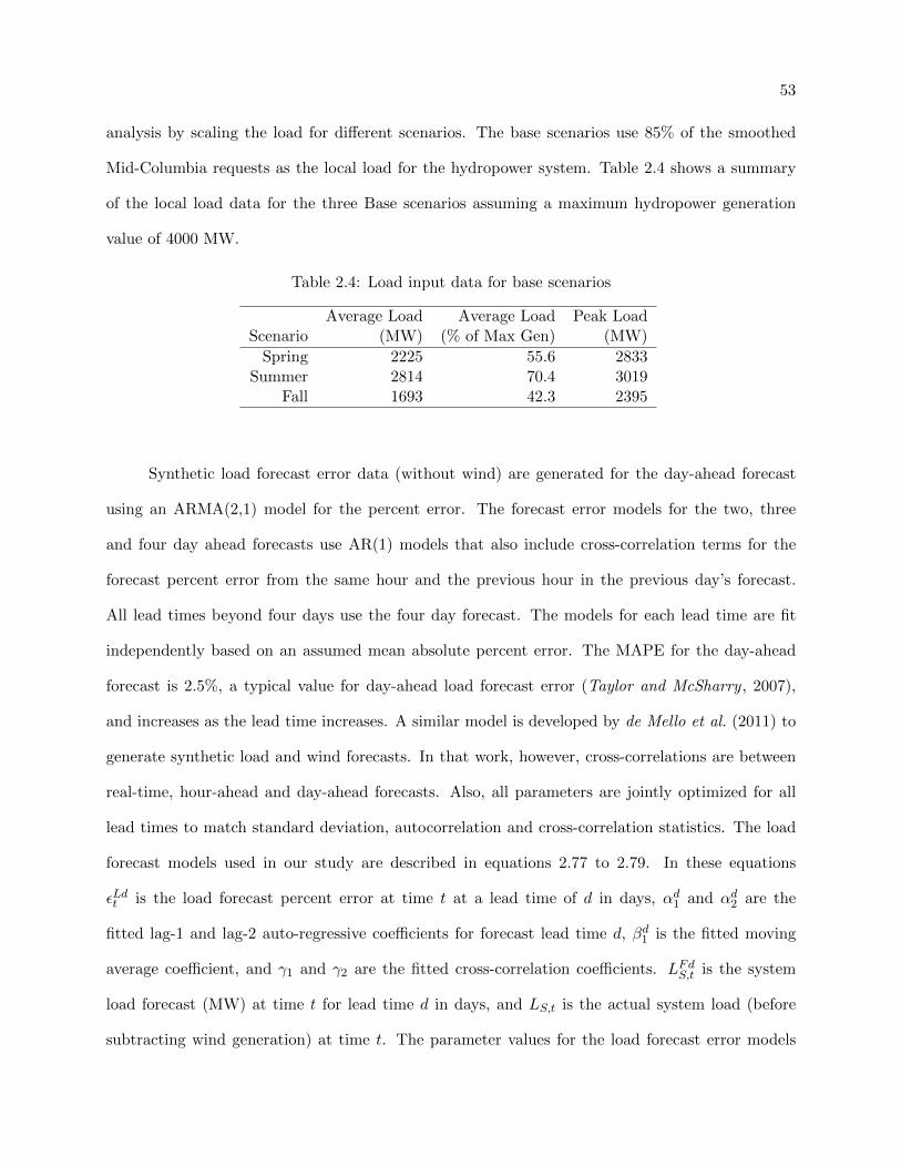
53

analysis by scaling the load for different scenarios. The base scenarios use 85% of the smoothed

Mid-Columbia requests as the local load for the hydropower system. Table 2.4 shows a summary

of the local load data for the three Base scenarios assuming a maximum hydropower generation

value of 4000 MW.

Table 2.4: Load input data for base scenarios

Average Load Average Load Peak LoadScenario (MW) (% of Max Gen) (MW)

Spring 2225 55.6 2833Summer 2814 70.4 3019

Fall 1693 42.3 2395

Synthetic load forecast error data (without wind) are generated for the day-ahead forecast

using an ARMA(2,1) model for the percent error. The forecast error models for the two, three

and four day ahead forecasts use AR(1) models that also include cross-correlation terms for the

forecast percent error from the same hour and the previous hour in the previous day’s forecast.

All lead times beyond four days use the four day forecast. The models for each lead time are fit

independently based on an assumed mean absolute percent error. The MAPE for the day-ahead

forecast is 2.5%, a typical value for day-ahead load forecast error (Taylor and McSharry , 2007),

and increases as the lead time increases. A similar model is developed by de Mello et al. (2011) to

generate synthetic load and wind forecasts. In that work, however, cross-correlations are between

real-time, hour-ahead and day-ahead forecasts. Also, all parameters are jointly optimized for all

lead times to match standard deviation, autocorrelation and cross-correlation statistics. The load

forecast models used in our study are described in equations 2.77 to 2.79. In these equations

εLdt is the load forecast percent error at time t at a lead time of d in days, αd1 and αd2 are the

fitted lag-1 and lag-2 auto-regressive coefficients for forecast lead time d, βd1 is the fitted moving

average coefficient, and γ1 and γ2 are the fitted cross-correlation coefficients. LFdS,t is the system

load forecast (MW) at time t for lead time d in days, and LS,t is the actual system load (before

subtracting wind generation) at time t. The parameter values for the load forecast error models

54

are shown in Table 2.5.

Day-ahead load forecast percent error:

εL1t = α1

1εL1t−1 + α1

2εL1t−2 +NL1

t

(0, σL1

)+ β1

1N1t−1

(0, σL1

)(2.77)

Two, three and four day ahead load forecast percent error:

εLdt = αd1εLdt−1 +NLd

t

(0, σLd

)+ γLd1 εLd−1

t + γLd2 εLd−2t−1 , d ∈ {2, 3, 4} (2.78)

LFdS,t = εLdt LS,t (2.79)

Table 2.5: Load forecast model parameters

Lead Time 1 Day 2 Days 3 Days 4-7 Days

α1 0.439 0.254 0.162 0.158α2 0.099 NA NA NAβ1 0.736 NA NA NAγ1 NA 0.656 0.391 0.376γ2 NA 0.141 0.629 0.588σ 0.015 0.025 0.008 0.008

MAPE 0.025 0.030 0.0325 0.035

The magnitude of the load forecast error is relatively small, particularly when compared to

the wind generation forecast error. While the general distribution of load forecast error is significant

because it contributes to the reserve requirement calculation (see Section 2.4.3.5), the hydropower

model is relatively insensitive to the specific trace of load forecast error. Only a single trace of load

forecast error is used, therefore, for each scenario whereas multiple traces of wind forecast error

are modeled. It is also important to note that it is the net load forecast (load forecast less wind

forecast) that is used as an input to the model, so within the model there is no distinction as to

whether a change in the net load forecast comes from the load forecast or the wind forecast.

2.4.3.2 Hydrologic Data

Inflow data for the hydropower system (modeled as outflow from Reservoir 1A) are taken

from Grand Coulee Dam hourly outflow data.26 This represents the fact that operators of run-of-

26 http://www.nwd-wc.usace.army.mil/ftppub/water quality/10data/

55

river hydropower systems often have to manage variable flows resulting from releases from upstream

hydropower dams. A perfect hydrologic forecast is assumed, however, for the one-week planning

horizon.

2.4.3.3 Wind Data

Wind generation inputs for the model are based on scaling observed wind generation data

from Bonneville Power Administration.27 Synthetic wind generation forecasts are produced using an

ARMA(2,1) model and a Box-Cox transformation of the forecast error for the day-ahead forecast.

For two-day-ahead and three-day-ahead forecasts, additional error is added by separate ARMA

models. The three-day-ahead forecast is used for all lead times of three to seven days. Chapter 3

provides a detailed description of the of the wind generation data and wind forecast model used

for this study. Multiple traces of wind generation forecasts are generated for each actual wind

generation time series. All other inputs to the model remain constant when running the multiple

wind generation forecast traces for a given scenario.

Four different wind penetration levels are modeled for each scenario: 10%, 20%, 30% and

40%, which correspond to installed wind capacities of 444 MW, 1000 MW, 1714 MW and 2667

MW respectively. The 40% wind penetration case is recognized as a relatively extreme penetration

scenario and is included in our study only to evaluate system behavior at the upper limits of wind

integration.

2.4.3.4 Price Data

The initial market clearing prices for energy and ancillary services (regulation down, regula-

tion up, spinning reserve, and non-spinning reserve) are taken from observed CAISO MCPs.28 29

Day-ahead hourly prices correspond to the same time periods in 2010 as the raw load, wind and

hydrologic data. For the scenarios which include a real-time energy market, the average hourly

27 http://transmission.bpa.gov/Business/Operations/Wind/default.aspx28 http://www.caiso.com/market/Pages/ReportsBulletins/ReportsBulletinsArchive/Default.aspx29 http://oasis.caiso.com/mrtu-oasis/?doframe=true&serverurl=http%3a%2f%2ffrptp09%2eoa%2ecaiso%2ecom

%3a8000&volume=OASIS

56

real-time MCPs from the same dates and hours in 2008 are used.30 These initial data are set as the

block 1 prices (PRE1,t see Section 2.3.4). Then each block of additional energy (or ancillary service

capacity) sold reduces the market clearing price by a fixed percentage (a parameter value). In

energy markets, all energy generation bids that are awarded are compensated at the same market

clearing price. In order to simulate this, PREb,t, which represents the unit price ($/MWh) of each

new block b of energy sold at time t, is reduced such that the average price across all used blocks

decreases by this fixed percentage. RE represents the reduction factor, the fixed percentage by

which the MCP decreases for each block.

b∑c=1

PREc,t

b=(1−RE

)b−1∑c=1

PREc,t

b− 1(2.80)

For example, if the initial unit price is $100/MWh, and the MCP is assumed to decrease 1% for

each additional block of energy, then the unit price for the second block would be $98/MWh so

that the average across both blocks is $99/MWh. This is defined by the following equation:

PREb,t = max(

0.01, PRE1,t(1−RE

)b−2 (1− bRE

)), b ≥ 2 (2.81)

The lower limit for the price of a given block is set at $0.01/MWh to prevent the optimization

solution from using the linear piecewise power segments out of order if the price were zero or

negative. In reality energy prices can become negative, primarily in the real-time market when

there is an excess of energy in the system. It can be assumed that if the model is selling energy at

$0.01/MWh, it represents a situation in which the hydropower system is being forced to produce

power at negative prices due to physical and/or policy constraints. A sample enregy value curve

and corresponding price curve are shown in Figure 2.6.

For energy, the prices are set for 50 MWh blocks. For day-ahead energy, the modeled MCP

decreases by 1% for each additional 50 MWh sold (RE = 0.01).31 The real-time market is assumed

to have less depth than the day-ahead market, and thus the reduction factor is set to 5% and

30 http://oasishis.caiso.com/index.jsp31 This is based on an a simplification and approximation of results observed by Jonsson et al. (2010) when

evaluating the impact of wind generation on energy prices in the Nord Pools Elspot market.

57

Figure 2.6: (a) Sample energy value curve and (b) corresponding price curve representing themarket depth for energy with an initial (block 1) MCP of $40/MWh and reduction factor (RE) of1%/50 MWh. Plot (b) represents the curve described by equation 2.81 and is the derivative of (a).

10% per 50 MWh for different scenarios. The prices for ancillary services are based on 10 MW

blocks, and the reduction factors are 4% per 10 MW for regulation down and 5% per 10 MW for

regulation up, spinning reserve, and non-spinning reserve. It is recognized that the shape of the

price curve for a given product can vary considerably from one market to another dependent on

a number of factors, particularly the mix of available generation resources and their associated

marginal costs. The parameter values we use here are only intended as a simplified example of the

effect of increased generation on market prices. The sensitivity to the price curve parameter for

the day-ahead energy market is tested by evaluating alternative scenarios in which this parameter

value is varied, including a scenario which assumes unlimited market depth (no change in prices

with increased generation).

The unit value of ancillary services deployment energy for regulation up, spinning reserve

and non-spinning reserve (PRX,Deplt see Equation 2.32) is set equal to the price of the first block of

real-time energy at time step t. For regulation down, the unit cost of deployment energy, CRD,Deplt ,

is set equal to the price of the first block of day-ahead energy at time step t. The unit value of

58

energy in storage, PREISt , is set equal to the daily average price of the first block of day-ahead

energy. Note that the EIS unit value does not affect the optimization solution, but it does impact

the relative contribution of the EIS value to the total system value. The total system value is

evaluated in post-processing of the model outputs; therefore different assumptions about the value

of EIS can be tested by simply scaling the final EIS value.32

2.4.3.5 Reserve Requirements

One of the primary effects of increased wind penetration on power systems is its impact

on reserve requirements for the system. In our study, reserve requirements are calculated outside

the model based on existing methods described below and imported as input data. There is no

attempt to optimize the amount of local reserves within the model. (See Morales et al., 2009;

Ortega-Vazquez and Kirschen, 2009; Leite da Silva et al., 2011, for alternative methods to establish

reserve quantities which optimize their value in the system.)

Contingency Reserve: The contingency reserve requirement we use here is based on the

WECC requirement that a reserve sharing group or BA that is not part of a reserve sharing group

carry a contingency reserve that is equal to the greater of the largest single potential contingency

in the BA, such as the sudden loss of the largest generating unit, or the sum of 3% of load and 3%

of generation (WECC, 2008). For base scenarios the contingency reserve requirement in our model

is set to 500 MW, which is assumed to represent the portion of the single largest contingency in the

BA that must be covered by the hydropower system.33 Alternative scenarios also test contingency

reserve requirements of 250 MW and 1000 MW. The WECC standard also states that at least half

of the required contingency reserve must be spinning reserve.

SRreqS,t = 0.5CRreqS,t (2.82)

32 While modifying the EIS unit value obviously changes the total system value, it was observed that this hadrelatively little impact on general trends and relative results between scenarios.

33 The 3% load plus 3% generation calculation typically results in a contingency reserve requirement under 200MW for our model.

59

Regulating Reserve: There are not formal regulatory requirements on regulating reserves.

Rather NERC sets maximum allowable area control error (ACE) based on deviations from the

standard frequency of 60 Hz (NERC, 2007). Each BA must then determine the amount of regulating

reserves it should maintain in order to assure that it will meet the NERC standards. The WWSIS

uses a regulation requirement of 1% of peak load within each transmission area (GE Energy , 2010).

The EWITS assumes 1% of total load to be approximately equal to three times the standard

deviation of load variability at the regulating time scale and uses this as the basis for the regulation

requirement. The variability of wind at this time scale is assumed to be negligible and thus does

not impact the regulation requirement (EnerNex , 2010). The regulating reserve requirement we

use here follows the EWITS approach of using 1% of load.34

RU reqS,t = RDreqS,t = 0.01LS,t (2.83)

Load Following Reserve: Load following reserve does not have an external requirement.

The method we use in this study for determining the load following requirement is based on methods

used in Acker et al. (2012b); Holttinen et al. (2008) and Robitaille et al. (2012). The total load

following reserve requirement, LF reqS,t , has two components. It is scheduled to assure that there is

sufficient capacity, both up and down, to balance longer time scale variability in net load. It is also

used in the day-ahead scheduling run to assure that there is sufficient capacity scheduled to cover

net load forecast error.

For the load variability component, LF reqNL∆, the requirement is based on the distribution

of hourly net load changes (LnetS,t − LnetS,t−1). The requirement is set equal to the absolute value of

the hourly net load change corresponding to a set exceedence probability.35 We use an exceedence

probability of 0.995. The variability component of the load following requirement is evaluated for

each calendar month.

34 The EWITS regulating reserve requirement also includes a term for wind forecast error. In our study, all windforecast error is assumed to be covered by load following reserve, and thus this additional term is not included in theregulation requirement.

35 It is also common to use 10-minute or 15-minute net load changes. Only hourly load data are available here.Also some methodologies use a multiple of standard deviations, often 3, in place of exceedence probability, but thiscan underestimate the magnitude of extreme events due to the non-Gaussian distribution (Acker et al., 2012b)

60

Reserve Capacity for Net Load Variability:

P(|LnetS,t − LnetS,t−1| ≤ LF

reqNL∆

)= 0.995 (2.84)

The forecast error component, LF reqNLFE , is similar. In the absence of empirical forecast data,

one hundred traces of day-ahead load and wind forecasts are generated for each month using the

synthetic forecast generators described in Sections 3.2 and 2.4.3.1 and observed wind and load

for that month. The load forecast error, εLt , and wind forecast error, εWt , (both in MW) are

then calculated and combined into the net load forecast error. The reserve requirement is again

calculated as the forecast error value (absolute) corresponding to an exceedence probability of 0.995.

Reserve Capacity for Net Load Forecast Error:

P(|εLt + εWt | ≤ LF

reqNLFE

)= 0.995 (2.85)

Assuming that these two components of load following are uncorrelated, the combined re-

quirement is calculated by taking the square root of the sum of the squares of the individual

requirements.

LF reqS,t =

√(LF reqNL∆

)2+(LF reqNLFE

)2(2.86)

The load following reserve requirement is removed in the operations run to simulate the use of the

reserve capacity to meet the actual load as it deviates from the forecast. The load following reserve

requirement is a critical parameter value in terms of how it impacts the results of wind integration

studies. The values used for load following reserve in our model are heavily influenced by the

assumptions that generation is being scheduled based on day-ahead forecasts and at an hourly time

step. In order to evaluate the sensitivity to these assumptions, alternative scenarios are run in

which load following reserve requirment is reduced. These scenarios use exceedence probabilities of

0.99 and 0.98 when establishing the load following reserve requirement. This could also be taken

as a proxy for modeling an improved wind forecast where the reduced forecast error results in a

reduction in the forecast error component of the reserve requirement.

61

A summary of the incremental reserve requirements for the spring base scenario is shown in

Table 2.6. Total reserve requirements for the summer and fall scenarios are within 4% of these val-

ues. Additional methodologies for determining operating reserve requirements for wind integration

studies are described in Holttinen et al. (2008) and Ela et al. (2010).

Table 2.6: Incremental reserve requirments, spring base scenario

Installed Regulation Up Contingency Load Following TotalPenetration Wind (MW) (Avg MW) Reserve (MW) Reserve (MW) (MW)

No Wind 0 22.2 500 303.3 825.610% 444 22.2 500 435.9 958.120% 1000 22.2 500 789.0 1311.230% 1714 22.2 500 1290.9 1813.240% 2667 22.2 500 1979.3 2501.5

2.4.3.6 Ancillary Services Deployment Energy

Regulation is assumed to correspond to random fluctuations in net load, and thus over a one-

hour time step net regulation deployment energy should be approximately zero. When modeled

as two separate reserve products, however, as we do here, the hourly average of each is non-zero.

For the scheduling run, the regulation up and regulation down deployment fractions are set to 0.2

for all time steps representing the average percentage of regulation capacity that is expected to

be deployed during operations. For the operations run, the deployment fraction is modeled as a

random normal variable.36 Like other model parameters, regulation deployment can vary from one

system to another. Only a single trace of regulation deployment is modeled for each scenario. The

sensitivity to regulation deployment is not evaluated in our study.

Whereas regulation is being deployed constantly, the contingency reserve is assumed to be

deployed much less frequently as it is only to cover major contingency events. When contingency

reserves are deployed, it is typically only for a short time period (WECC, 2008). For the schedul-

36 Values for the mean and standard deviation are based on an analysis of regulation data from thePJM market for May4-8, 2009; available at http://pjm.com/markets-and-operations/ancillary-services/mkt-based-regulation/archived-mkt-based-regulation.aspx

62

ing run the spinning reserve is assigned a deployment fraction of 0.02, and non-spinning has a

deployment fraction of 0.01 to represent how much the reserve is assumed to be deployed over the

long-term for planning purposes. In the operations run, however, the deployment fraction for each

is set to 0. No contingency event occurs during the run period. The one exception is a single

scenario that is run to test the system response to a large contingency event. In this case the

deployment fraction for both spinning and non-spinning reserve is set to 0.9 for a single time step

representing a 450 MW loss of generation within the BA.

2.4.4 Scenario Descriptions

As stated previously, the impacts and value of integrated wind generation and hydropower

are dependent on a large number of factors and can vary significantly with seasonal conditions.

Many existing wind integrations studies run scenarios for a complete year or multiple years to

evaluate the effects over a large range of conditions, often to arrive at an average cost of wind

integration. Our approach here is to model specific weeks to evaluate the sensitivity of wind and

hydro integration to changes in system conditions with variations in select system parameters. This

allows the effects of specific seasonal conditions to be analyzed. Descriptions of the scenarios used

to carry this out are given here.

2.4.4.1 Base Scenarios: Full Policy

Three weeks are selected which have different hydrologic and wind conditions as well as

having different seasonal non-power constraints in effect. These are modeled with the full policy

set in place for the Base scenarios.

Spring Scenario: May 14-20, 2010

The first scenario is intended to model relatively average stream flow. A minimum spill

requirement for fish passage is in effect for the final three reservoirs (8 kcfs at Reservoir 1D and 20

kcfs at Reservoirs 1E and 1F). A seasonal minimum environmental flow of 65 kcfs is required at

Reservoir 1F. The daily outflow fluctuation at Reservoir 1F is limited to 20 kcfs.

63

Summer High Flow and High Wind Scenario: June 22-28, 2010

The second scenario represents a high flow scenario with high wind generation, often one

of the critical operating conditions for hydropower systems with integrated wind generation. The

excess water flowing through the system can increase the need to run the hydropower plants as

near to capacity as possible. This can reduce the flexibility for balancing wind generation. While

this scenario is constrained by physical conditions, it is the least restricted by non-power policy

constraints. In this scenario, minimum spill requirements are in effect for all five dams (15 kcfs at

Reservoirs 1B and 1C, 20 kcfs at Reservoirs 1D and 1E, and 25 kcfs at Reservoir 1F), although the

reservoirs tend to spill in excess of the minimum even without added wind generation due to the

high flows in the system. The maximum allowable spill for TDG limits is increased to 100 kcfs at

each dam (75 kcfs at Reservoir 1D). This tends to be the most controlling constraint on the system

in this scenario. The maximum allowable daily outflow fluctuation at Reservoir 1F is increased to

40 kcfs.

Fall Scenario: October 30-November 5, 2010

The third scenario is marked by the restricted outflow range at Reservoir 1F during daylight

hours (55 kcfs-70 kcfs) to protect spawning salmon (based on spawning season requirements in

the Hanford Reach Fall Chinook Protection Program Executed Agreement (2004)). This constraint

affects scheduling throughout the system as reservoirs must position themselves during nighttime

hours to be able to meet the narrow flow requirements for the following day. This is also the most

water limited scenario. There is no minimum spill requirement.

2.4.4.2 Reduced Policy Scenarios

In order to evaluate the impact of modeling non-power policy, the baseline scenarios are

compared to the same scenarios with two levels of simplified policy sets. The only non-power con-

straints in effect for the Unconstrained case are minimum and maximum pool elevations, constant

minimum outflows (10 kcfs) for all reservoirs and target ending storages. The Moderate Policy case

adds minimum spill and minimum seasonal environmental flow requirements. All power-related

64

constraints and objectives are in place for all policy cases. It is necessary to clarify that the re-

duced policy cases are included only to show the importance of accounting for non-power policy

when modeling hydropower systems. They are not included to suggest alternative operating policy

for the hydropower system.

2.4.4.3 Effects of Wind Forecast Error, Wind Variability and Wind Energy

The effects of adding wind generation to the power system are divided into three components:

energy, variability and forecast error. The effects of the added energy are assumed to be positive in

general (though in certain circumstances, particularly high-flow seasons, excess energy can create

difficulties for the system). Added energy in the system means more water can be stored in the

hydropower reservoirs and used for generation when most beneficial. It can also mean that more

energy is available to sell for increased revenue. In general, over a long-term average, wind variability

and forecast error are assumed to have negative impacts on the system. The negative impacts are a

combination of the increased reserve requirements due to variability and forecast error (see Section

2.4.3.5) and the direct impacts such as the increased ramping and starts and stops from variability

or the shifting of operations away from peak efficiency due to forecast error. In the short-term for

specific scenarios, however, they may be observed to benefit the system, such as if the variability

happens to match up with demand patterns or peak pricing.

In order to isolate the effects of these three components of integrated wind generation, within

each scenario four separate cases are modeled: A No Wind case; a Full Wind case37 which includes

wind generation in the net load including forecast error in the scheduling run; a No Error case38

which includes wind generation but uses a perfect wind forecast in the scheduling run; and a No

Variability case which includes the equivalent amount of wind energy but without the variability

and without forecast error. The net value from each isolated component of wind generation can

37 Each case with wind is modeled at all four penetration levels.38 No Error here refers to wind forecast error only. Load forecast error is still included in all cases.

65

then be calculated as shown in equations 2.87 to 2.89.

NetWindForecastErrorV alue = TotalV alue(FullWind)− TotalV alue(NoError) (2.87)

NetWindV ariabilityV alue = TotalV alue(NoError)− TotalV alue(NoV ariability) (2.88)

NetWindEnergyV alue = TotalV alue(NoV ariability)− TotalV alue(NoWind) (2.89)

Dividing each net value by the total wind generation at the given penetration gives the average

value of each component per unit of wind generation. Other model outputs can be compared in the

same manner. For example, any difference in spill between the Full Wind case and the No Error case

can be assumed to be due to wind forecast error. For the No Variability case, rather than model

the added wind energy as a constant flat block, the equivalent amount of wind energy over the

one-week scenario is shaped to approximately follow the load with a ramping rate approximately

equal to that of a coal plant. The energy resource ramps from 60% capacity during low load hours

to 100% capacity over the hours 5:00 to 9:00 and then back down to 60% over the hours 18:00 to

22:00. A sample time series plot of the No Variability case compared to actual wind for the same

scenario is shown in Figure 2.7.

2.4.4.4 Alternative Scenarios for Sensitivity Analysis

In addition to the scenarios described above, the sensitivity of the results to select modeling

assumptions and parameter values is evaluated by running alternative scenarios described here. In

general, these sensitivities are tested in the spring scenario only, unless specified otherwise.

Real-time market: Two scenarios include a real-time market in the operations run ap-

proximated by hourly energy prices. These scenarios are used to evaluate effects of the assumption

that all generation is scheduled based on day-ahead forecasts. The availability of a real-time market

allows additional capacity scheduled as reserves to be utilized to generate revenue once real-time

conditions are known. The two scenarios differ only in their price curve parameters. In one the

real-time energy price decreases 5% per 50 MWh of energy sold. In the second the price decreases

10% per 50MWh.

66

Figure 2.7: Time series of actual wind (solid line) and the corresponding No Variability wind(dashed line) for the same scenario at 30% penetration

Load following reserve requirement: Two alternative scenarios use exceedence prob-

abilities of 0.98 and 0.99 to calculate the load following reserve requirement (see Section 2.4.3.5).

(The Base case uses an exceedence probability of 0.995.) These scenarios test the sensitivity to

a major assumption that all reserves are scheduled based on day-ahead forecast error characteris-

tics. This can be interpreted as an approximation of either scheduling generation and reserves in

a shorter time horizon or scheduling based on improved forecasts. The forecasts are not actually

altered in these scenarios. Only the load following requirement is changed.

Load levels: High and low local load cases are modeled for both the spring and summer

scenarios. The High Load case uses 100% of the smoothed Mid-Columbia request data. The Low

Load case uses 50% of the smoothed Mid-Columbia request. A summary of the load inputs for

these scenarios is shown in Table 2.7.

Transmission constraints: Available transmission is one of the primary constraining

factors for large scale wind integration (EnerNex , 2010). A scenario with the transmission limit

raised to 2500 MW (from the 1500 MW Base case) is modeled for the spring and summer scenarios,

67

Table 2.7: Load input data for alternative load level scenarios

Base Case High Load Case Low Load Case

Avg Avg Peak Avg Avg Peak Avg Avg PeakScenario (MW) (% Max) (MW) (MW) (% Max) (MW) (MW) (% Max) (MW)

Spring 2225 55.6 2833 2617 65.4 3333 1309 32.7 1667Summer 2814 70.4 3019 3311 82.8 3552 1655 41.4 1776

and unlimited transmission is modeled for the summer scenario to evaluate the extent to which

transmission becomes a critical constraining factor in this model.

Low load and increased transmission: The 2500 MW and unlimited transmission cases

are combined with the low load case for the spring and summer scenarios to further explore the

sensitivity of the results to transmission limits, particularly when there is excess energy in the

system.

Market depth: For a Low Market Depth case the day-ahead energy price is reduced by

2% per 50 MWh (from the Base case of 1% per 50 MWh). An Unlimited Market Depth case is also

modeled where the price at a given time step does not change regardless of the amount of energy

sold.

Contingency reserve: The contingency reserve requirement is reduced to 250 MW (from

the Base case of 500 MW) for one scenario and raised to 1000 MW for another scenario to test

the sensitivity to the assumption about how much contingency reserve the hydropower system is

required to carry.

Contingency event: A contingency event is modeled that represents the loss of a 450

MW generator in the BA at noon on the fifth day of the run, during a period when the wind is

ramping down. This scenario is to evaluate the flexibility of the system to actually provide the

necessary balancing generation. Placing the contingency event at the first time step of one of the

six hour operations runs prevents any forecast knowledge of the event in the optimization solution

so that the system cannot re-position itself to prepare for the contingency event.

68

Wind timing: In order to test the effects of the wind timing in relation to load and energy

prices, scenarios are run with the wind generation and corresponding forecast shifted back 6, 12

and 18 hours. These scenarios intentionally violate the principle of maintaining time-synchronized

data in order to specifically evaluate the sensitivity to the timing of inputs.

Summer hydrology with spring prices: The summer scenario is run with spring energy

and ancillary services price inputs in order to evaluate the extent to which the changes in system

behavior between the spring and summer scenarios are due to the different hydrologic and wind

conditions and how much is simply due to different prices. Like the wind timing scenarios, this

scenario intentionally violates the principle of maintaining time-synchronized data.

2.5 Assumptions and Simplifications

In addition to assumptions and simplifications that have been mentioned in the previous

sections, it is important to identify the following assumptions that affect the model results as well

as some points on what our methodology does not do.

• Operational costs for ancillary services, such as increased maintenance costs due to wear

on equipment, are not included due to lack of sufficient data to model such costs. See

Piekutowski et al. (2012) for a description of the sources of potential costs to hydropower

resources from increased ancillary services use.

• The hydropower resources in our model are assumed to provide all of the reserves that are

required from the integrated wind generation. In some systems, a portion of these reserves

may come from thermal resources such as gas turbines.

• The wind generators are not assumed to make any payments for the ancillary services

required to balance the wind variability and uncertainty. Some systems may have payment

mechanisms in place for such services.

• There are no transmission constraints within the modeled utility. In reality there may

be geographic constraints on reserve requirements within a BA related to transmission

69

constraints that require certain levels of reserve capacity within specific geographic regions

of the BA and not only within the BA as a whole.

• Hydropower unit outages are not considered.

• Each scenario run is deterministic. A single wind generation forecast corresponds to a

single realized wind generation time series. Though multiple traces of wind forecast are

modeled for each scenario, there is no stochastic optimization within the model.

• Our methodology does not directly model unit commitment or economic dispatch of other

generating resources outside of the integrated hydropower and wind system. The effects

of a different mix of generating resources in the system are assumed to be approximated

by different load and market depth scenarios, though how these scenarios correspond to

specific generation portfolios is not explored in depth here.

• Our approach does not make a comparison to wind integration without coordinated hy-

dropower as a balancing reserve as is done in some integration studies (see, for example,

Angarita and Usaola, 2007; Benitez et al., 2008; Matevosyan et al., 2009). Rather it uses

hydropower without integrated wind generation as the Base case then assesses the net value

of wind added to the hydropower system. It does not assess the value of hydropower for

balancing wind.

Chapter 3

Wind Generation Modeling

The response of a hydropower system to integrated wind generation depends in part on the

amount of installed wind capacity and the total wind generation. It also depends on characteristics

such as the variability in wind generation, wind forecasting methods and the resulting forecast

error, and the timing of wind generation relative to peaks in load and energy prices. All of these

characteristics, in addition to the installed wind capacity, can vary significantly for different geo-

graphic regions and for each integrated wind and hydropower system. The methodology we present

here does not attempt to model hydropower and wind integration under all possible conditions

and wind characteristics. Rather an attempt is made to model realistic scenarios of actual wind

generation and wind forecast error recognizing that these represent only a small sample of possible

wind generation scenarios and specific results could vary when evaluating wind integration in other

systems. A sensitivity analysis is carried out to partially evaluate the effects of varying certain

characteristics of the wind inputs. This includes shifting the timing of the wind generation and

reducing the amount of reserve capacity scheduled to cover wind forecast errors which would ac-

company a reduction in wind forecast error. Details of this sensitivity analysis are discussed further

in sections 2.4.4.4 and 4.5.3.

71

3.1 Actual Wind Generation Data

The wind generation data used in this study are based on Bonneville Power Administration

(BPA) Balancing Authority total wind generation in 2010.1 Numerous wind integration studies

have used synthetic wind generation data for actual wind inputs as well as synthetic wind forecast

inputs. In the WWSIS, the level of wind capacity to be modeled was well beyond current installed

capacity, and thus wind generation time series inputs were simulated based on weather models

and power characteristics of sets of wind turbines assumed to be located at selected wind farm

locations (GE Energy , 2010). The BPA data are used here for several reasons. First it is a readily

available set of actual generation data for an aggregated set of wind farms which contains true

characteristics of wind generation. The BPA installed wind capacity from 2010 is approximately

equal to the installed capacity for the 40% penetration case, the highest wind penetration case

modeled in our study, and thus there is not a need to produce additional synthetic wind data.

Also these wind generation data come from the same region as the hydrologic input data. It can

be assumed, then, that correlations that may exist between hydrologic conditions and wind are

being captured in these datasets. In addition, much of the BPA wind generation is used to meet

California RPS requirements and can therefore have an impact on energy prices in the CAISO

market. Using the BPA wind data and the CAISO price data as inputs to our model captures this

correlation as well.

Wind penetration can be defined differently for different BAs. Often it is calculated as

installed wind capacity as a percent of peak load. Like the BPA balancing area, the system we

model here is a net exporter of energy. In this case it is more reasonable to define penetration in

terms of installed wind as a percent of peak generation instead of peak load. In our model the peak

generation is defined as the maximum hydropower generation plus the maximum wind capacity.

The expression for wind penetration is then

Wpen =PWpen,max

PWpen,max + PHmax(3.1)

1 http://transmission.bpa.gov/Business/Operations/Wind/default.aspx

72

where Wpen is wind penetration, PWpen,max is the installed wind capacity at the given penetration,

and PHmax is the maximum hydropower generation. (Note that the maximum hydropower generation

is less than the nameplate capacity.) The installed wind capacity based on a set penetration level

is then calculated as

PWpen,max =PHmaxWpen

1−Wpen(3.2)

The modeled wind penetration cases are 10%, 20%, 30% and 40%. The assumed maximum hy-

dropower load is assumed to be 4000 MW. The corresponding installed wind capacity amounts are

then 444 MW, 1000 MW, 1714 MW and 2667 MW respectively.

The BPA data are available in five minute intervals and are averaged to hourly values then

scaled to represent the desired wind penetration levels used in our study. It is widely recognized

that wind generation variability does not remain constant as the level of penetration changes. As

increased wind capacity is brought online, the geographical distribution generally increases resulting

in less correlation in outputs between individual wind generators; therefore the relative variability

for large amounts of wind generation is less than for smaller amounts (Wan, 2004, 2005). In order

to account for this it is necessary to scale the variability in the wind data in addition to scaling

the mean. The total BPA wind capacity in 2010 was approximately equal to the 40% wind case in

our model. It is therefore necessary to increase the variability from the scaled, observed data for

the lower penetration scenarios in order to account for the reduced geographic distribution of wind

generation resources associated with decreased installed capacity.

The BPA wind generation data are only available in aggregate, so there are no direct means by

which to determine the effect on variability of removing portions of the wind resources and reducing

the geographic distribution. As a substitute, to estimate a reasonable change in variability, wind

data from select sites in the WWSIS dataset are used.2 The WWSIS dataset provides ten minute

simulated wind data for sites in the western United States based on weather conditions for 2004,

2005, and 2006. Only the 2006 data are used in our analysis. WWSIS sites are selected such

2 The WWSIS dataset is provided by the National Renewable Energy Laboratory, which is operatedby the Alliance for Sustainable Energy, LLC for the U.S. Department Of Energy and is available athttp://www.nrel.gov/wind/integrationdatasets/western/data.html.

73

that the total annual mean generation and the annual standard deviation of wind generation at

ten minute intervals are approximately equal to the BPA 2010 mean and ten-minute standard

deviation (σ10). Then sites are removed from the selected WWSIS sites so that the annual mean

generation is equal to that of the 30%, 20%, and 10% wind cases in our model. With each reduction

the geographic spread of the wind sites is decreased which has the effect of increasing the relative

variability.3 The four cases based on the WWSIS data are then converted to hourly wind data,

and the annual 60-minute standard deviation (σpen60 ) is calculated for each as well as the 60-minute

standard deviation for the BPA wind data (σBPA60 ). The ratio of the synthetic 60-minute standard

deviation to the BPA 60-minute standard deviation is then used to scale the deviation of wind

generation from the scaled mean at each time step.

First the mean wind generation value, PWpen, for the given penetration level pen is calculated

from the installed capacity for that penetration level and an assumed capacity factor for wind, FC ,

which is set to 0.3, a typical capacity factor for wind generation.

PWpen = PWpen,maxFC (3.3)

To calculate the “actual” wind generation, PWpen,t at time t a second term is added to the mean

generation value which represents the scaled deviation from the mean and incorporates the scaled

variability.

PWpen,t = PWpen +

σpen60

σBPA60

(PWBPA,t − P

WBPA

)(3.4)

σpen60 is the standard deviation of 60-minute wind generation for penetration pen based on the

WWSIS data, and σBPA60 is the BPA 60-minute standard deviation. PWBPA,t is the observed BPA

wind generation at time t, and PWBPA is the mean observed BPA wind generation. Appendix B

contains a listing of the WWSIS sites used to estimate the standard deviation for each penetration

case.

3 The relative variability can be measured by the coefficient of variation, the standard deviation divided by themean: COV = σ/µ. Details from this variability analysis including the WWSIS sites used and the resulting mean,standard deviation and COV values are shown in Appendix B.

74

3.2 Wind Generation Forecast

The integrated hydropower and wind generation modeling methodology presented in Chap-

ter 2 requires wind generation forecasts ranging from day-ahead to seven days ahead. Wind gener-

ation forecast data at these lead times are not available for the actual BPA wind generation data

that are used as the basis for the wind generation inputs into our model. In the absence of real

forecast data, synthetic wind generation forecasts are produced based on a statistical analysis of

combined observed actual wind generation data and wind generation forecast data made available

from a set of sample wind farms for the months of August through October. It is recognized that

the characteristics of wind generation forecast error can vary from one system to another and may

depend on a number of factors including installed wind capacity, geographic distribution of wind

generation resources, regional weather patterns, season, and forecasting methodologies employed.

The goal with the synthetic wind generation forecast methodology we present here is not to re-

produce wind generation forecasts that match those that would have corresponded to the actual

BPA wind generation data. Rather the purpose is to produce synthetic wind forecast time series,

given an actual wind forecast time series, that provide a reasonable and realistic characterization

of real wind generation forecast error recognizing that the specific characteristics of forecast er-

ror may be different for other systems. The analysis is carried out on the forecast percent error

normalized by the installed wind capacity so that the statistical characteristics can be transferred

to another system with a different level of installed capacity and different actual wind generation

characteristics.

3.2.1 Existing Statistical Wind Forecast Methodologies

Statistically-based synthetic wind forecast models have been developed previously for use in

wind integration studies. Two relevant examples, both of which use autoregressive moving average

(ARMA) models, are described here.

75

Soder (2004) develops an ARMA(1,1) model to produce synthetic wind speed forecast errors

for a single wind generation site. An optimization routine is used to fit the ARMA model parameters

with an objective of minimizing the squared difference between root mean squared error (RMSE)

from the model and RMSE in observed forecasts summed over a range of lead times. This model

is applied by Matevosyan et al. (2009) to develop a scenario tree of forecast errors, which when

added to a given wind speed forecast, provides a scenario tree of possible wind speed outcomes.

The wind speed forecast data are converted to wind generation forecasts based on modeled wind

turbine characteristics. The wind forecast and scenario tree are subsequently used in a stochastic

optimization algorithm to optimize the coordinated operation of a hydropower system and wind

farm.

de Mello et al. (2011) present a similar ARMA(1,1) model for wind generation forecast

errors with several key differences. They define three separate ARMA models each with their

own parameter values for real-time (5 minutes ahead), hour-ahead and day-ahead wind generation

forecast errors. The hour-ahead model includes a cross-correlation term which correlates the hour-

ahead forecast error with the real-time error from the same time step. The day-ahead model contains

a similar term to correlate the error with the hour-ahead model. An optimization algorithm then

fits parameters for all three models simultaneously. The other key difference is that the objective

for the fitting algorithm does not only minimize the differences between model and observed mean

error values. Rather it minimizes a weighted combination of the differences in observed and model

values for mean, standard deviation, auto-correlation and cross-correlation. In this manner, it

attempts to capture more of the statistical characteristics of forecast error beyond the mean alone.

3.2.2 Analysis of Observed Wind Generation Forecast Error

The two ARMA models mentioned in section 3.2.1 assume that wind generation forecast

errors are normally distributed with a mean of zero. Hodge and Milligan (2011) show that forecast

errors in shorter time frames (five minutes to three hours) are not Gaussian but rather have a higher

kurtosis than a normal distribution. In general, a normal distribution would underestimate the

76

number of time periods with very small and very large forecast error, and it would over predict the

number of time periods with moderate forecast error. de Mello et al. (2011) also mention that the

real-time forecast error distribution has more small errors and fewer large errors (greater kurtosis)

than a normal distribution and that the distributions for longer time scales are not symmetric, but

all of the distributions are assumed to be approximately Gaussian when applying the forecast error

model.

The actual wind generation data that have been provided from sample wind farms are at ten

minute intervals. These ten-minute data have been averaged into hourly values. The corresponding

wind generation forecast data are at fifteen minute intervals. At each interval a wind generation

forecast is given for each hour from one hour out to 72 hours out. From these fifteen minute data,

forecasts at the top of each hour have been extracted for lead times of 12, 24, 36, 48, 60 and 72

hours and are paired with the corresponding averaged hourly actual generation for that forecast

hour. The actual generation is subtracted from the forecast at each hour and for each lead time to

produce the forecast error. These error values are then normalize by dividing by the installed wind

capacity to produce a time series of wind generation forecast error as a percent of installed capacity

for each selected lead time. Histograms of the normalized forecast error at each lead time overlaid

with fitted normal distributions are shown in Figure 3.1. Statistics of the normalized forecast error

distributions for each lead time are displayed in Table 3.1.

Table 3.1: Statistics of normalized observed wind generation forecast error over a range of leadtimes

Lead Time 12 hr 24 hr 36 hr 48 hr 60 hr 72 hr

MAPE 0.2120 0.2166 0.2169 0.2270 0.2238 0.2280Mean -0.0219 -0.0259 -0.0305 -0.0355 -0.0416 -0.0414

Standard Deviation 0.2780 0.2843 0.2804 0.2968 0.2879 0.2923Skew -0.1664 -0.1780 -0.2542 -0.1331 -0.2381 -0.2877

Kurtosis 0.5054 0.4790 0.1893 0.3756 0.2070 0.0412Lag-1 Auto-correlation 0.8497 0.8844 0.8798 0.8829 0.8806 0.8911Lag-2 Auto-correlation 0.6599 0.6961 0.6875 0.6969 0.6976 0.7137

The histograms in Figure 3.1 demonstrate that the forecast errors do not conform to a normal

77

Figure 3.1: Histograms of observed wind generation forecast error (normalized by installed windcapacity) at a range of lead times overlaid with a normal distribution fitted to the data

distribution. Observation of the statistics in Table 3.1 reveals a positive kurtosis indicating that

the distribution is more peaked than a normal distribution and has heavier tails. (Note that the

kurtosis values displayed here are technically the excess kurtosis, the kurtosis in exceedence of

the kurtosis of a normal distribution, which is always 3.) Additionally the forecast error has a

negative skew as well as a negative mean, which becomes increasingly negative as the lead time

increases. This indicates that the forecast methodology employed for this system has a slight bias

to under predict the wind generation. The hourly forecast errors also exhibit a strong lag-1 and

lag-2 auto-correlation.

While the hydropower scheduling methodology employed for our study optimizes resources

based on net load forecasts for an entire week, generation is only scheduled for a 24 hour horizon,

so the model is most sensitive to the characteristics of the day-ahead forecast. It is therefore on the

78

day-ahead forecast that the attention is focused in developing the synthetic forecast methodology.

Also it is necessary to point out that a day-ahead forecast would technically be a forecast for 24

hours with lead times ranging from 12 to 36 hours (assuming that generation is scheduled at noon

for the following calendar day, which is typical for many day-ahead energy markets). Observation of

the error distributions for the 12 hour, 24 hour and 36 hour forecasts, however, shows that there are

only minor differences in the distributions across these lead times. Using the 24 hour forecast error

characteristics as a basis for developing a day-ahead forecast error model is therefore considered a

reasonable approximation.

3.2.3 Day-ahead Wind Forecast Model

Analysis of the observed forecast error data suggests that existing ARMA models could be

improved upon to capture some of the non-Gaussian characteristics of the error distribution. The

wind forecast model we employ applies a Box-Cox transformation to the error data before fitting an

ARMA model to the transformed error. As described below, this allows a standard ARMA model

with a random normal variable to be used to generate a forecast time series with errors that are

not normally distributed.

First the forecast error is normalized by the installed capacity.

εWt,obs =PWFt,obs − PWtPWmax

(3.5)

In equation 3.5, εWt,obs is the observed normalized wind forecast error, PWFt,obs is the observed 24 hour

lead time wind generation forecast (MW) for time t, and PWt is the actual wind generation (MW)

at time t. PWmax is the installed wind capacity (MW). Then the Box-Cox transformation is applied

to the normalized forecast error.

ε′t,obs =

(εWt,obs + λ2

)λ1− 1

λ1(3.6)

ε′t,obs in equation 3.6 is the transformed error, and λ1 and λ2 are parameters of the Box-Cox

transformation. The mean is then removed resulting in a distribution that is approximately normal

79

centered on a mean of zero.

ε∗t,obs = ε′t,obs − µ

′(3.7)

µ′

is the mean of the transformed error, and ε∗t,obs is the mean-removed transformed error to which

the ARMA model is fitted. The resulting distributions before and after the Box-Cox transformation

are shown in Figure 3.2.

Figure 3.2: Histograms overlaid with normal distributions and QQ-Normal plots of observed windforecast error and Box-Cox transformed error

80

ARMA models up to order (2,2) are then fit to the mean-removed transformed data, and

the model with the lowest AIC score is selected as the best fit. A general ARMA model of order

(p,q) is shown in equation 3.8 where the α and β coefficients are parameters, and N is a random

normal variable with mean of 0 and standard deviation of σ. AIC scores from the model fitting

and parameter values of the best fit ARMA(2,1) model and the Box-Cox transformation are shown

in Tables 3.2 and 3.3.

εt = α1εt−1 + α2εt−2 + . . .+ αpεt−p + β1Nt−1 (0, σ) + . . .+ βqNt−q (0, σ) +Nt (0, σ) (3.8)

Table 3.2: ARMA model fitting AIC values

Order ARMA(p,q) AIC

(1,0) -2029.53(1,1) -2303.87(1,2) -2316.41(2,0) -2345.96(2,1) -2357.30(2,2) -2299.87

Table 3.3: Wind forecast error model Box-Cox and ARMA(2,1) parameter values

Parameter λ1 λ2 α1 α2 β1 σ′

µ′

Value 1.255 1.331 1.526 -0.650 -0.364 0.128 0.326

The ARMA(2,1) model has the lowest AIC score and is therefore used to generate synthetic

Box-Cox transformed forecast error.

ε∗t,model = α1ε∗t−1,model + α2ε

∗t−2,model + β1Nt−1

(0, σ

′)

+Nt

(0, σ

′)

(3.9)

ε′t,model = ε∗t,model + µ

′(3.10)

The error term from the model is then transformed back and applied to the actual wind generation

at the given time step to produce the initial wind forecast value, PWF ′t,model.

εWt,model =(ε′t,modelλ1 + 1

)1/λ1− λ2 (3.11)

81

pWF ′t,model = PWt + εWt,modelP

Wmax (3.12)

The resulting forecast value is checked for feasibility. If the initial forecast value is negative or

greater than capacity, the forecast value, PWFt,model, is set to zero or maximum capacity respectively.

The values of ε∗t,model and Nt

(0, σ

′)

are then adjusted to correspond to this forecast value before

applying the ARMA model for the next time step.

pWFt,model =

0, pWF ′

t,model < 0

pWF ′t,model, 0 ≤ pWF ′

t,model ≤ PWmax

PWmax, pWF ′t,model > PWmax

(3.13)

Figure 3.3 displays the histograms of the observed 24 hour forecast error and 100 traces of

forecast errors generated by applying the forecast model to the same actual wind generation time

series. The corresponding statistics are presented in Table 3.4.

Figure 3.3: Histograms of observed wind generation forecast error and 100 traces of modeled forecasterror normalized by installed wind capacity

The results in Table 3.4 indicate that the forecast error model produces less variance in the

error outputs than the observed forecast error. It also has a resulting mean that is slightly positive

whereas the observed forecast error has a slightly negative mean, and the model skew is not as

negative as the observed skew. The model does a better job of reproducing the excess kurtosis than

82

Table 3.4: Statistics of observed and model forecast percent error distributions (Model values aremean values from 100 traces.)

Observed Model

MAPE 0.216 0.164Mean -0.025 0.042

Standard Deviation 0.284 0.213Skew -0.185 -0.010

Kurtosis 0.487 0.639Lag-1 Auto-correlation 0.884 0.847Lag-2 Auto-correlation 0.696 0.630

would occur if a normal distribution were assumed, and it does a relatively good job of capturing

the lag-1 and lag-2 auto-correlation. Additional analysis suggests that the differences in mean,

variance and skew come from the fact that the forecast model does not capture the dependency of

forecast error on the actual generation. In cases where the actual wind generation is low, an actual

wind forecast will tend to over-predict rather than under-predict the generation. The opposite is

the case when actual generation is high. The model does not tend to capture the magnitude of the

negative forecast errors very well in the case of high actual wind generation. Further analysis on

this is presented in Appendix B.

The wind generation forecast model (equations 3.9 to 3.13) is then applied to the actual

wind generation time series for the 10% penetration case for each scenario to be modeled using

the parameter values from Table 3.3. The resulting percent error from each trace is then used

to calculate the forecast value for each of the remaining penetration levels. The 10% penetration

case has the greatest relative variability, so using this actual wind generation series to generate the

forecast error time series assures that infeasible values do not result when scaling the forecast from

one penetration level to another. This allows the forecast percent error to remain constant across

all penetration levels for a given forecast trace within a given scenario. A time series plot of the

actual wind and a single trace of the day-ahead forecast for the spring scenario 30% penetration

case is shown in Figure 3.4.

83

Figure 3.4: Sample trace of model forecast wind generation and actual generation, spring scenario,30% penetration

3.2.4 Wind Forecast Models for Two and Three Days Ahead

For the two day ahead forecast error, εW2t,model, an additional error term, ε∆2

t,model is added to

the day-ahead forecast error at that time step.

εW2t,model = εWt,model + ε∆2

t,model (3.14)

The additional error term is generated by an ARMA model based on the differences between

observed 48 hour and 24 hour forecasts, ε∆2t,obs.

ε∆2t,obs = εW48

t,obs − εW24t,obs (3.15)

In this case the additional error is assumed to be normally distributed. Once again an ARMA(2,1)

model has the lowest AIC score and is selected as the best model. The model parameters are shown

in Table 3.5.

The three day ahead forecast error model is similar. An additional error term is added to

the two day error.

εW3t,model = εW2

t,model + ε∆3t,model (3.16)

84

where the observed differences between the 72 and 48 hour forecast error are used to fit the model.

In this case an AR(2) model has the lowest AIC score and is used to generate the additional three

day forecast error. Histograms of observed forecast error for lead times of 48 and 72 hours along

with results from 100 traces of model forecast error for the same lead times (representing two day

ahead and three day ahead forecasts) are shown in Figure 3.5 with the corresponding statistics in

Table 3.6.

Table 3.5: Parameter values for additional error models for two day ahead and three day aheadwind generation forecasts

α1 α2 β1 σ µ

Two-day Forecast 0.329 0.270 0.543 0.066 -0.0078Three-day Forecast 0.930 -0.132 NA 0.068 -0.0067

Figure 3.5: Histograms of observed and model 48 hour and 72 hour wind generation forecast errornormalized by installed capacity

85

Table 3.6: Statistics of observed and model 48 hour and 72 hour wind generation forecast errornormalized by installed capacity

48-hour 2-day 72-hour 3-dayObserved Model Observed Model

MAPE 0.227 0.176 0.228 0.193Mean -0.035 0.052 -0.041 0.064

Standard Deviation 0.297 0.226 0.292 0.243Skew -0.133 -0.040 -0.288 -0.056

Kurtosis 0.376 0.685 0.041 0.563Lag-1 Auto-Correlation 0.883 0.828 0.891 0.820Lag-2 Auto-Correlation 0.697 0.608 0.714 0.605

The two day ahead model is applied to the day ahead forecast traces used as inputs for the

integrated hydropower and wind model to generate the corresponding two day ahead forecast for

each trace. The same is done with the three day forecast. The three day ahead forecast for a given

trace is used for all lead times of three days or more for that trace.

Chapter 4

Assessing the Value of Integrated Hydropower and Wind Generation

4.1 Introduction

4.1.1 Overview

The rapid growth in installed wind generation capacity in recent years puts greater de-

mand on power systems to maintain sufficient flexible generating resources and balancing reserves.

Hydropower has often been considered one of the best balancing resources to couple with wind

generation. Hydro generators have high ramp rates and often have automatic generation control

(AGC) capabilities enabling quick response to imbalances in energy supply and demand. Hy-

dropower generation has a low marginal cost, and the fuel supply, water, is a renewable resource.

Most conventional hydropower facilities also have the capability to store energy in the form of

impounded water allowing for a level of control over the timing of generation, making use of the

energy when most needed.1 Hydropower, therefore, plays an increasingly valuable role as part of

a sustainable energy portfolio by not only producing renewable energy itself, but also by making

it possible to incorporate larger amounts of other renewable generation, such as wind, through the

flexible balancing resources (ancillary services) it provides.

Unlike other power generating resources, however, hydropower facilities are generally designed

and operated to serve multiple objectives. These objectives may include flood control, environmen-

1 Pumped storage hydropower facilities (PSH) provide the added benefit of using excess energy for pumping waterto an upper reservoir to be used for generation in times of higher energy demand thus providing additional balancingreserves. Only conventional hydropower is considered in our study, though the methodology could be extended tosystems with PSH.

87

tal objectives including habitat protection and fisheries management, water storage and delivery,

navigation, water quality and recreation in addition to power generation. The specific objectives

and their relative priorities are unique to each system, but in general water objectives have a

higher priority in system operating policy than the power objectives. That is to say that the water

management objectives cannot be compromised for power generation purposes. These non-power

policies restrict the allowable outflows from hydropower facilities effectively reducing system flexi-

bility. It is necessary to account for this reduced flexibility from non-power policy when evaluating

the capacity of the hydropower system for balancing integrated wind generation.

4.1.2 Existing Wind and Hydropower Integration Studies

In 2011, the International Energy Agency (IEA) Task 24 Integration of Wind and Hydropower

Systems Final Technical Report was released (Acker , 2011a,b). This report brings together case

studies from participants in seven countries to investigate wind integration in electric systems

with large amounts of hydropower generation. It analyzes benefits, challenges and impacts of

wind integration in systems with varied characteristics in their market structures, hydropower

systems and electrical systems. A summary of the case studies and their findings is presented in

Acker et al. (2012b) and shows that in many cases existing hydropower systems can provide the

balancing reserves necessary for integrating large amounts of wind generation. Some case studies

expect significant operational challenges for high levels of wind penetration (greater than 20%). A

review of existing literature on wind and hydropower integration, including studies which focus on

developing scheduling algorithms for coordinated hydropower and wind generation is provided in

Chapter 1.

One other large-scale study of note in regards to wind and hydropower integration is the

Western Wind and Solar Integration Study which evaluates the feasibility and impacts of up to

30% wind and 5% solar in the WestConnect footprint (GE Energy , 2010). The WWSIS shows a

significant increase in operating costs for the entire system if the flexibility of hydropower resources

for balancing the variability of renewable generation is removed. One common conclusion from

88

both the IEA Task 24 Report and the hydropower analysis from the WWSIS is that there is a

need for improved hydropower modeling in wind integration studies. In a companion study that

carries out a detailed analysis of the hydropower modeling in the WWSIS, Acker and Pete (2012)

find that modeling assumptions at times lead to an overestimation of true hydropower capacity,

particularly in low flow years. In another companion report to the WWSIS, Hodge et al. (2011) note

the importance of modeling non-power constraints when trying to accurately capture the impacts

of wind generation on hydropower systems. The IEA Task 24 Report calls for improvements in the

modeling of both physical processes, such as mass balances, and constraints on the system (Acker

et al., 2012b).

4.1.3 Significance of this Research

The research we present here contributes to improved hydropower modeling for wind inte-

gration studies by developing a methodology that not only models the physical processes of the

hydropower system but also accounts for the limitations resulting from both power-related and

non-power policy constraints. The methodology utilizes the optimization solver in RiverWare, a

hydropower modeling tool, to model hydropower operations with a set of prioritized policy con-

straints and objectives based on realistic policies that govern the operation of actual hydropower

systems. This captures the effective capacity and flexibility of a hydropower system that must be

considered by system operators when coordinating hydropower resources with wind generation.

In addition to realistic modeling of hydropower operations and policy, the methodology also

produces an economic evaluation of integrated wind and hydropower that not only accounts for the

value of energy from the integrated system but also for the value of ancillary services provided by

the hydropower resources. With the relatively recent development of markets for ancillary services

in many regions, ancillary services can carry an explicit economic value in addition to their value

in maintaining grid stability. Ancillary services can provide a significant portion of hydropower

revenue and should therefore be accounted for when determining the total value of the system.

The end value of integrated hydropower and wind generation is specific to each power system

89

and is dependent on numerous factors. In consideration of this, the goal here is not to establish a

specific value for integrated wind generation. The point is rather to demonstrate the importance

of modeling realistic hydropower operations, including non-power constraints, when considering

the value of integrated hydropower and wind generation. In addition the sensitivity of the value of

wind integration to various conditions and system parameters is evaluated. To do this, the proposed

methodology is applied to a sample hydropower system with integrated wind generation under a

range of scenario conditions. By comparing effects on economic outputs, operational conditions and

constraint satisfaction from modifying various system parameters, conclusions are drawn about key

modeling assumptions and system characteristics and their effect on the evaluation of hydropower

and wind integration.

4.2 Modeling and Methodology

4.2.1 Conceptual Model

The manner in which a hydropower system is scheduled and operated is dependent to a

significant degree on the organizational structure of the larger system of which it is a part and the

market structures which exist in the system’s balancing authority area (BA). The organizational

model we propose here is a hybrid of a traditional, vertically integrated utility and a formal energy

market. The hydropower system is a sub-system within a BA, such as a large-scale utility which

owns multiple hydropower resources. These resources must be dispatched to meet local load and

reserve requirements. Additional capacity can be utilized to bid into formal markets for energy and

ancillary services. Such a mixed model is representative of organizational structures in the Western

Electricity Coordinating Council (WECC) area where power producers must meet load obligations

in their own BA but also have the opportunity to participate in the California Independent System

Operator (CAISO) market (Loose, 2011). Energy markets improve conditions for integrating large

amounts of wind generation by providing sub-hourly energy markets that redispatch every five to

fifteen minutes (Milligan et al., 2009). In our model, participation in the market occurs in only

90

one direction. Energy and ancillary services can be sold into the market when the hydro system

has excess capacity, but they cannot be purchased from the market to help meet local requirements

when capacity is limited. All resources to meet local requirements must come from within the

system being modeled. All modeling is at an hourly time step. All sub-hourly processes are

therefore approximated by hourly averages.

The utility is assumed to have must-take contracts with a set of geographically dispersed

wind farms. Wind is incorporated into the model as negative load. One important note is that

no explicit economic value is assigned to the energy and reserves used to meet the local load and

reserve requirements. Meeting load and reserve requirements is treated as a constraint for the

system. Only the energy and ancillary services sold into the market are given an explicit economic

value. Also wind is not assigned a purchase cost. Rather the output returns the net value of added

wind generation by comparing the total value from a Base case without added wind generation to

the same scenario with wind generation. This is in contrast to many previous studies which have

used flat blocks of equivalent wind energy without the variability as the base case to establish the

cost of wind integration. Milligan and Kirby (2009) address the issues with using the flat wind

block approach.

4.2.2 Hydropower Modeling in RiverWare

4.2.2.1 RiverWare Optimization

Hydropower modeling for our study is carried out using the optimization solution in River-

Ware, a general tool for hydropower, river and reservoir system modeling developed at the Center

for Advanced Decision Support for Water and Environmental Systems (CADSWES) at the Uni-

versity of Colorado. RiverWare’s optimization solution is a pre-emptive linear goal program in

which the user creates prioritized goals, which are constraints and objectives that represent the

operating policy of the system. Then a linear program is solved at each priority level. When the

goal is written as a soft constraint (or multiple soft constraints), the objective function of the linear

91

program at that priority is to minimize the deviations from the constraint values. In the case that

not all soft constraints at a given priority level can be satisfied the optimization minimizes the

maximum deviation then re-solves the linear program until all constraints at that priority are satis-

fied (known as a repeated minimax solution). Once a soft constraint has been satisfied at a higher

priority, it will not be violated to meet a lower priority soft constraint or objective. This approach

accounts for the fact that not all policy constraints are of equal importance. For example target

environmental flow constraints may not be satisfied if it would require violating license minimum

or maximum storages (pool elevations), but environmental flow constraints will be satisfied before

optimizing power generation. Additional information about optimization in RiverWare, including

the formulation of automatic physical constraints, is provided by Eschenbach et al. (2001).

4.2.2.2 Power Modeling

Hydropower generation is modeled at the plant level as a function of operating head and

turbine release. Each plant’s power characteristics are represented by a set of piecewise linear

curves, one for each operating head, with linear interpolation between curves to calculate power at

intermediate operating heads. In the optimization solution, operating head is held constant at a

user-input estimated value. A post-optimization simulation run uses portions of the optimization

solution to set releases. It then uses an iterative solution to calculate the operating head and power

generation. This removes the approximation error introduced by assuming a constant operating

head in the optimization solution.

4.2.2.3 Ancillary Services

The classification of ancillary services or operating reserves varies in different regions (Ela

et al., 2011). Four marketable ancillary services are defined in our model, consistent with the

ancillary services products available in the CAISO market: regulation up, regulation down, spinning

reserve and non-spinning reserve. Load following reserve is a fifth ancillary service that is modeled

only as a local resource and represents all other reserve capacity scheduled to balance any variability

92

or forecast error in the net load beyond the regulation time scale. Load following reserve is modeled

as a bi-directional reserve and carries the same incremental and decremental capacity. In general,

the incremental reserves at a hydropower plant are constrained by

RUr,t + SRr,t +NSr,t + LFr,t ≤ HCr,t − Pr,t (4.1)

where RUr,t, SRr,t, NSr,t and LFr,t represent regulation up capacity, spinning reserve, non-spinning

reserve and load following reserve respectively, HCr,t represents maximum hydropower capacity at

time t and Pr,t represents hydropower generation at time t. HCr,t is a function of the operating head

and the maximum turbine release at that operating head. Decremental reserves are constrained by

RDr,t + LFr,t ≤ Pr,t − Pminr,t (4.2)

where RDr,t is regulation down capacity, and Pmr,tin is the minimum allowable generation at the

plant. Additional constraints in the policy set further restrict the hydro capacity at certain hy-

dropower plants based on flow restrictions from non-power constraints. This captures the manner

in which non-power policy effectively limits the flexibility of certain hydropower plants in providing

ancillary services.

If reserve capacity is actually deployed to generate energy (or to reduce generation in the

case of regulation down), then this quantity of energy is removed from the reserve capacity to avoid

double counting the reserves. The deployment of ancillary services at time scales shorter than one

hour, such as regulation, cannot be modeled directly. Instead a deployment fraction is used to

represent the fraction of the reserve that is deployed in actual generation on average over the time

step. For further details on the ancillary services modeling, refer to Section 2.3.3.

4.2.2.4 Economic Modeling

The value of energy sold at a given time step is based on a piecewise linear function. For

each additional block of energy, the unit value decreases. This represents the effect that bidding

additional energy that has a low marginal cost (e.g. wind energy or hydropower) has on reducing the

93

market clearing price. Because the day-ahead energy bid comes from the scheduling run using day-

ahead wind forecasts (as described in 2.2), this also approximates the effect high wind generation

forecasts can have on reducing energy prices (see Jonsson et al., 2010). The economic value of

each ancillary service (regulation up, regulation down, spinning reserve and non-spinning reserve)

is modeled similarly to energy using a piecewise linear function; however the value of ancillary

services also includes the compensation for the energy generated when the reserve capacity is

deployed. The deployment value is based on the real-time market clearing price for energy.

4.2.2.5 Other Physical Processes

RiverWare provides the capability to model numerous physical processes in the hydropower

system. Among those included in our model are reservoir mass balances and pool elevations, rout-

ing between reservoirs and tailwater elevation. Refer to Zagona et al. (2001) and the RiverWare

Documentation (CADSWES , 2012) for details on how these processes are modeled within River-

Ware. Section 2.4 contains details on the specific methods used in our model for this study and

the parameter values within the model.

4.2.3 Run Sequence

The model run sequence consists of a two-stage optimization which is intended to represent

actual operations where generating resources are scheduled based on net load forecasts then must

be adjusted to meet real-time conditions. First a one week scheduling run is carried out using

wind generation forecasts and load forecasts as inputs. This is followed by a 24 hour operations

run which uses actual wind generation and load inputs. The objective of the scheduling run is to

maximize the combined value of energy and ancillary services sold in the day-ahead market for the

entire week after meeting all constraints, including target ending elevations for each reservoir, as

well as local load and reserve requirements. The purpose of the one-week scheduling run is for the

system to look far enough into the future to position itself to be able to meet anticipated conditions

when scheduling for the current day.

94

A set of outputs from the first 24 hours of the scheduling run are passed to the operations

run. These include energy and ancillary services committed into the day-ahead market, generation,

reserves and releases scheduled at each hydropower plant and scheduled pool elevations at each

reservoir at the end of each six hour period for the next 24 hours. The objective of the operations

run is to maximize the value of energy in storage. The operations run is divided into four individual

six hour runs. This division into six hour runs balances a representation of reasonable flexibility

of the hydro resources to adjust generation based on updated forecasts without an overestimation

of system flexibility from modeling perfect forecast knowledge over the entire 24 hour run period.

Alternative scenarios include a real-time market in the operations run with an objective to maximize

the value of energy sold in the real-time market. After the operations run, the model advances 24

hours with the ending reservoir storages becoming the new initial conditions. Updated load and

wind forecasts are imported before starting a new one-week scheduling run. The process is repeated

to produce one full week of operations run outputs. The model run sequence is described in greater

detail in Section 2.2.

4.3 Wind Modeling

4.3.1 Actual Wind

Wind generation data are based on Bonneville Power Administration (BPA) Balancing Au-

thority 2010 total wind generation data.2 BPA five minute data are averaged to hourly values for

use in our study and then scaled to represent the desired wind penetration levels: 10%, 20%, 30%,

and 40%. The 40% wind penetration case is recognized as a relatively extreme penetration scenario

and is included here only to evaluate system behavior at the upper limits of wind integration. Wind

variability does not remain constant as the level of penetration changes. The wider geographical

distribution of wind farms typically associated with increased penetration results in less correlation

between generators and thus reduced relative variability (Wan, 2004, 2005). In order to account

for this, the variability in the wind data is scaled as well as the mean. The total BPA wind capacity

2 http://transmission.bpa.gov/Business/Operations/Wind/default.aspx

95

from 2010 is approximately equal the capacity for the 40% penetration case in our model. The

relative variability is therefore increased from the scaled observed data for the lower penetration

scenarios. The BPA wind generation data are only available in aggregate, so wind data from select

sites in the WWSIS 2006 dataset3 are used to estimate a reasonable change in variability. WWSIS

sites are selected such that the total annual mean generation and the annual standard deviation of

wind generation at ten minute intervals are approximately equal to the BPA 2010 mean and ten

minute standard deviation. Then sites are removed from the selected WWSIS sites so that the

annual mean generation is equal to that of the 30%, 20%, and 10% wind cases. With each reduction

the geographic spread of the wind sites is decreased which has the effect of increasing the relative

variability. The four cases based on the WWSIS data are then converted to hourly wind data,

and the annual 60-minute standard deviation is then calculated for each as well as the 60-minute

standard deviation for the BPA wind data. The ratio of the synthetic 60-minute standard deviation

to the BPA 60-minute standard deviation is then used to scale the deviation of wind generation

from the scaled mean at each time step.

PWpen,t = PWpen +

σpen60

σBPA60

(PWBPA,t − P

WBPA

)(4.3)

PWpen = PWpen,maxFC (4.4)

PWpen,t is the “actual” wind generation value at time t for the given penetration level pen. σpen60 is

the 60-minute standard deviation for penetration level pen based on the WWSIS wind data, and

σBPA60 is the BPA 60-minute standard deviation. PWBPA,t is the observed BPA wind generation at

time t. PWpen,max is the installed wind capacity for penetration pen, and FC is the wind generation

capacity factor which is assumed to be 0.3 for all penetration levels.

3 The WWSIS dataset is provided by the National Renewable Energy Laboratory, which is operatedby the Alliance for Sustainable Energy, LLC for the U.S. Department Of Energy and is available athttp://www.nrel.gov/wind/integrationdatasets/western/data.html

96

4.3.2 Wind Forecast

In the absence of real forecast data corresponding to the BPA actual wind generation, syn-

thetic wind generation forecasts are produced based a statistical analysis of combined observed

actual wind generation data and wind generation forecast data from a set of sample wind farms.

The goal with the synthetic forecast model we use here is not to reproduce forecasts that match

those corresponding to the actual BPA wind generation data. Rather the purpose is to produce

synthetic wind forecast time series that provide a reasonable and realistic characterization of wind

generation forecast error recognizing that the specific characteristics of forecast error may be dif-

ferent for each system.

Previous wind integration studies have used autoregressive moving average (ARMA) mod-

els to produce synthetic wind forecasts. Matevosyan et al. (2009) employ an ARMA(1,1) model

developed in Soder (2004) to develop a scenario tree of forecast errors for a stochastic optimiza-

tion algorithm. The ARMA model parameters are fit to minimize the deviation in RMSE from

observed forecast error over a range of forecast lead times. de Mello et al. (2011) develop a similar

ARMA(1,1) model for wind generation forecast errors. The fitting of this model, however, also

accounts for the cross-correlation between forecast errors at various time frames. The model is fit

to minimize the weighted difference in observed and model values for mean, standard deviation,

auto-correlation and cross-correlation with the forecast error series of shorter time frame.

ARMA models assume that the forecast error is normally distributed. Hodge and Milligan

(2011) show that forecast errors in shorter time frames (five minutes to three hours) are not Gaussian

but rather have higher kurtosis than a normal distribution. In general, a normal distribution would

underestimate the number of time periods with very small and very large forecast error, and it would

over predict the number of time periods with moderate forecast error. Analysis of the forecast error

from the sample wind farms similarly reveals a kurtosis greater than that of normally distributed

error as well as a negative skew (see Figure 4.1). In order to better capture these characteristics

in our model, a Box-Cox transformation is first applied to the forecast error data, and then an

97

ARMA model is fit to the mean-removed transformed data. An ARMA(2,1) model has the lowest

AIC score and is thus used for the synthetic forecast model.

The observed normalized wind generation forecast error, εWt,obs is defined as

εWt,obs =PWFt,obs − PWtPWmax

(4.5)

where PWFt,obs is the observed wind power forecast at time t, PWt is the actual wind power, and PWmax

is the maximum wind power (installed capacity). A Box-Cox transformation is then applied to

the normalized error with λ1 and λ2 as parameters, and the mean of the transformed error, µ′, is

removed.

ε′t,obs =

(εWt,obs + λ2

)λ1− 1

λ1(4.6)

ε∗t,obs = ε′t,obs − µ

′(4.7)

The ARMA(2,1) model with fitted parameters α1, α2, β1 and σ′

is then used to generate traces of

the Box-Cox transformed forecast error.

ε∗t,model = α1ε∗t−1,model + α2ε

∗t−2,model + β1Nt−1

(0, σ

′)

+Nt

(0, σ

′)

(4.8)

ε′t,model = ε∗t,model + µ

′(4.9)

The error term from the model is then transformed back and applied to the actual wind generation

at the given time step to produce the wind forecast.

εWt,model =(ε′t,modelλ1 + 1

)1/λ1− λ2 (4.10)

pWFt,model = PWt + εWt,modelP

Wmax (4.11)

The resulting forecast value is checked for feasibility. If the forecast is negative or greater than ca-

pacity, the forecast value is set to zero or maximum capacity respectively. The values of ε∗t,model and

Nt

(0, σ

′)

are then adjusted to correspond to this forecast value before applying the ARMA model

for the next time step. The fitted model parameters are shown in Table 4.1. Histograms comparing

100 traces of the model forecast error distribution to the observed forecast error distribution are

shown in Figure 4.1 with the corresponding statistics in Table 4.2.

98

Table 4.1: Wind forecast error model Box-Cox and ARMA(2,1) parameter values

Parameter λ1 λ2 α1 α2 β1 σ′

µ′

Value 1.255 1.331 1.526 -0.650 -0.364 0.128 0.326

Figure 4.1: Histograms of observed wind generation forecast error and 100 traces of modeled forecasterror normalized by installed wind capacity

Table 4.2: Statistics of observed and model forecast error distributions normalized by installedcapacity (Model values are mean values from 100 traces.)

Observed Model

MAPE 0.216 0.164Mean -0.025 0.042

Standard Deviation 0.284 0.213Skew -0.185 -0.010

Kurtosis 0.487 0.639Lag-1 Auto-correlation 0.884 0.847Lag-2 Auto-correlation 0.696 0.630

The ARMA(2,1) model is then applied to the wind generation time series used in our inte-

grated wind and hydropower model scenarios. If it is assumed that power generation is scheduled

at noon for the following calendar day, then a true day-ahead forecast would actually span lead

times of 12 to 36 hours. Analysis of the observed forecast error data, however, shows little change in

mean absolute percent error in forecasts with lead times ranging from 12 to 72 hours. Thus using a

99

24 hour lead time forecast is considered here as a reasonable approximation of a day-ahead forecast.

For forecasts of lead times greater than one day, an ARMA(2,1) model is applied to generate the

additional error added to the 24 hour error. In this case, it is assumed that the additional error has

a normal distribution. Because the scheduling run is scheduling generation for the next 24 hours

only, the hydropower model is most sensitive to the day-ahead forecast and much less so to the

characteristics of forecasts with longer lead times.

4.4 Test Case

4.4.1 Physical Hydropower System

The described methodology is applied to a test case system of five hydropower plants on

a single river with a combined nameplate capacity of approximately 5000 MW and an assumed

maximum load of 4000 MW. A single inflow to the system is modeled. The cascading reservoir

system has limited storage, approximately two days of typical flow, but the size of the individual

reservoirs varies significantly from 12,760 acre-feet to 168,720 acre-feet. This variation in storage

capacity impacts how the system must be operated. For example, Reservoir 1D, the third power

reservoir in the system, has very little storage and is therefore operated essentially as a run-of-

river hydropower plant. For this reason, it is excluded from providing ancillary services. All

reserves, therefore, must be provided by the remaining four hydropower projects. A depiction of

the RiverWare model is shown in Figure 4.2.

4.4.2 Policy

The policy set for the hydropower system has a general priority order that sets licensing

constraints (minimum and maximum pool elevations) at the highest priority. These are followed by

non-power water and environmental policy objectives and then the power objectives to meet load

and reserve requirements and to maximize the economic value of energy and ancillary services. A

summary of the policy is provided here.

100

Figure 4.2: RiverWare model workspace showing 5 hydropower projects in a cascading reservoirsystem; Reservoir 1A is a storage reservoir and is included here only to provide the inflows to thehydropower system.

4.4.2.1 Non-power Policy

In reality, each hydropower system has non-power policies unique to that system that limit

its operations. While the specific policies vary from one system to another, the common result in

regards to hydropower operations is that the non-power policy, in general, reduces the flexibility

with which the hydropower system can be operated to meet power objectives. The non-power

policy implemented in our model is representative of policy constraints in the Pacific Northwest,

though it is not the actual policy of any individual system. Constraints are based on policies such

as those coming from biological opinions and other agreements in place primarily to improve fish

101

survival rates in the hydropower system. Examples of constraints in the policy set include:

• Minimum flow requirements at all reservoirs with higher minimum flow requirements which

vary seasonally for the final downstream reservoir.

• Minimum spill requirements at all reservoirs in the spring and summer to improve fish

passage.

• Maximum spill limits at all reservoirs used as a proxy for limits on total dissolved gas

(TDG) concentration.

• Limits, which vary seasonally, on the difference between the daily minimum and maximum

outflow at the final downstream reservoir.

• Limits on the hourly change in tailwater elevation at the final downstream reservoir.

• Meeting target ending storage levels.

• Minimum pool elevations for recreational purposes at the two largest reservoirs. (Note

that this constraint actually comes at a priority below meeting local load and reserve

requirements but before the objective to maximize the value of energy and ancillary services

sold into the market.)

A number of the policy constraints apply to the final reservoir, 1F, which must re-regulate

the flow passing through the hydropower system. This is typical of many hydropower systems.

Due to the essentially run-of-river nature of this system, however, constraints on this reservoir have

impacts on operations throughout the system.

4.4.2.2 Power Policy and Reserve Requirements

Power-related policy includes constraints to meet load, reserve (ancillary services) require-

ments and minimum generation requirements for station service at each reservoir. The operations

run also includes additional soft constraints to use the power schedules for each hydropower plant

102

from the scheduling run within the tolerances of the scheduled load following reserve and regulation

capacity. The use of soft constraints represents the flexibility of the hydropower system to adjust

operations to meet real time conditions. The minimax solution, however, will force the actual

generation to be as close to the schedule as possible while meeting all higher priority constraints.

This prevents the hydropower system from completely re-optimizing during the operations run to

meet the new load and thus represents the loss of efficiency that generally occurs when the system

must deviate from its schedule to meet changing conditions.

Increased balancing reserve requirements are typically seen as the primary source of wind

integration costs, and thus the determination of reserve requirements is a key factor in wind inte-

gration studies. Ela et al. (2010) provide a summary of how balancing reserves have been calculated

in previous wind integration studies. The requirement for regulation capacity, both up and down,

used in our model is based on the method used in the Eastern Wind Integration and Transmission

Study (EnerNex , 2010). The regulating reserve requirement is set to 1% of load which is assumed

to be approximately three standard deviations of the one-minute variability separated from the 20-

minute rolling average. Wind variability is assumed to be insignificant at this timescale and thus

does not contribute to the regulation capacity requirement.4 For base scenarios the contingency

reserve requirement is set to 500 MW which is assumed to represent the portion of the single largest

contingency in the BA that must be covered by the hydropower system. A minimum of 50% of

the contingency reserve must come from spinning reserve (WECC, 2008). In alternative, scenarios

contingency reserve requirements of 250 MW and 1000 MW are modeled.

In our model, all increases in reserves due to wind are incorporated into the load following

reserve requirement. Load following reserve is scheduled to assure there is sufficient capacity,

both up and down, to balance longer time scale variability in net load and net load forecast

error. Assuming that these two components of load following are uncorrelated, the combined

requirement is calculated by taking the root sum of squares of the individual requirements. For

4 The EWITS also includes a term for wind forecast error in the regulating reserve requirement. In our model allincreases in reserves due to wind forecast error are incorporated into the load following reserve.

103

the variability component, the requirement is set equal to the absolute value of the hourly net load

change corresponding to an exceedence probability of 0.995 (see Acker et al., 2012b; Holttinen et al.,

2008; Robitaille et al., 2012) and is evaluated for each calendar month. The forecast error component

is similar. In the absence of empirical forecast data, one hundred traces of day-ahead load and wind

forecasts are generated for each month using the synthetic forecast generators described in Sections

3.2 and 2.4.3.1. These are then combined into net load forecasts, and the reserve requirement

is calculated as the absolute error magnitude associated with an exceedence probability of 0.995.

Alternative scenarios are tested using exceedence probablilities of 0.99 and 0.98. The load following

reserve requirement is removed in the operations run to simulate the use of the reserve capacity to

meet the actual load as it deviates from the forecast.

LF reqS,t =

√(LF reqNL∆

)2+(LF reqNLFE

)2(4.12)

P(|LnetS,t − LnetS,t−1| ≤ LF

reqNL∆

)= 0.995 (4.13)

P(|εLt + εWt | ≤ LF

reqNLFE

)= 0.995 (4.14)

The economic objective comes at the final priority. For the scheduling run the objective is to

maximize total revenue, the combined value of day-ahead energy and ancillary services (capacity and

deployment energy value) after meeting all non-power constraints, load and reserve requirements

and target ending storages. In addition to the aforementioned constraints, this objective is also

subject to a static transmission constraint which limits the combined energy and ancillary services

that can be sold into the market. The transmission constraint applies only to energy and ancillary

services being sold into the market. No transmission constraints are modeled within the hydropower

system. The transmission capacity for the baseline scenarios is 1500 MW. Alternative scenarios are

also modeled to test the effects of increased transmission capacity.

The objective for the operations run is to maximize the ending energy in storage value after

meeting all power and non-power constraints and meeting minimum ending storage targets at each

reservoir. The energy in storage metric represents the generating potential of a unit of water as it

passes through all downstream hydropower plants and thus gives a higher weight to water stored

104

farther upstream in the system. Alternative scenarios implement a real-time energy market in the

operations run, and in these cases the objective is to maximize the value of energy sold into the

real-time market.

4.4.3 Scenarios

The impacts and value of integrated wind generation and hydropower are dependent on a

large number of factors and can vary significantly with seasonal conditions. Many previous wind

integration studies run scenarios for a complete year or multiple years often to arrive at an average

cost of wind integration. The approach we present here is to model specific weeks to evaluate the

sensitivity to varied conditions and system parameters. This allows the effects of specific seasonal

conditions to be analyzed.

4.4.3.1 Base Scenarios: Full Policy

Three weeks are selected which have different hydrologic and wind conditions as well as

having different seasonal non-power constraints in effect. These are modeled with the full policy

set in place for the Base scenarios.

Spring Scenario: May 14-20, 2010

The first scenario is intended to model relatively normal stream flow. A minimum spill

requirement for fish passage is in effect for three of the five reservoirs. A seasonal minimum

environmental flow of 65 kcfs is required at the final reservoir, 1F. The daily outflow fluctuation at

Reservoir 1F is limited to 20 kcfs.

Summer High Flow and High Wind Scenario: June 22-28, 2010

The second scenario represents a high flow scenario with high wind generation, often one of the

critical operating conditions for hydropower systems with integrated wind generation. The excess

water flowing through the system can increase the need to run the hydropower plants near capacity,

which can reduce the flexibility for balancing wind generation. While this scenario is constrained

by physical conditions, it is the least restricted by non-power policy constraints. Minimum spill

105

requirements are in effect for all five reservoirs. The maximum allowable spill for TDG limits is

increased to 100 kcfs at each dam (75 kcfs at Reservoir 1D). The maximum allowable daily outflow

fluctuation at Reservoir 1F is increased to 40 kcfs.

Fall Scenario: October 30-November 5, 2010

The third scenario is marked by a restricted outflow range at Reservoir 1F during daylight

hours (55 kcfs-70 kcfs) to protect spawning salmon. This constraint affects scheduling throughout

the system. This is also the most water limited scenario.

4.4.3.2 Simplified Policy Scenarios

In order to evaluate the impact of modeling non-power policy, the Base scenarios are compared

to the same scenarios with two levels of simplified policy sets. The only non-power constraints in

effect for the Unconstrained case are minimum and maximum pool elevations, constant minimum

outflows for all reservoirs and target ending storages. The Moderate Policy case adds minimum

spill and seasonal environmental flow requirements. All power-related constraints and objectives

are in place for all policy cases.

4.4.3.3 Isolated Effects of Wind Forecast Error, Wind Variability and Wind Energy

The effects of adding wind generation to the power system are divided into three components:

energy, “predictable” variability and forecast error. In general added wind energy is considered to

have a positive impact while variability and forecast error have negative impacts, though in certain

cases the opposite may be true in the short term. In order to evaluate the isolated effects of these

components each Base scenario is also run without wind forecast error and then without wind

variability. All other inputs, including load forecast error, remain the same as the Base case. For

the No Variability case, rather than model the added wind energy as a constant flat block, the

equivalent amount of wind energy over the one-week scenario is shaped to approximately follow the

load in a regular diurnal pattern with a ramping rate approximately equal to that of a coal plant.

This represents a generating resource that is able to add energy to system when, in general, it is

106

beneficial. Comparing the No Forecast Error case with the Base case with forecast error isolates

the impacts of wind forecast error, comparing the No Variability case with the No Forecast Error

case isolates the impacts of predictable wind variability, and comparing the No Variability case

with the No Wind case isolates the effects of wind energy.

4.4.3.4 Alternative Scenarios for Sensitivity Analysis

In recognition of the fact that wind integration effects are specific to each system and sce-

nario conditions, a sensitivity analysis is carried out on select conditions and parameters within

the scenarios described above. A description of specific characteristics that are evaluated in the

sensitivity analysis is given in Section 4.5.3.

4.4.4 Input Data

In order to create realistic scenarios, input data for load, wind, prices and inflows are based

on synchronized actual observed data from select weeks in 2010 as described here. Inflow data are

taken from Grand Coulee Dam hourly outflow data.5 This represents the fact that operators of

run-of-river hydropower systems often have to manage variable flows resulting from releases from

upstream hydropower projects. Load data are based on Mid-Columbia hourly combined non-federal

request data. The Mid-Columbia request data display greater intra-hour variability than typical

load for a BA, so a five hour rolling average is applied to smooth the data. This results in a load

profile that is more representative of a typical load. The data are scaled for different scenarios

to evaluate the sensitivity to various levels of local load. Synthetic load forecasts are generated

using an ARMA(2,1) model for the day-ahead forecast similar to the synthetic wind forecast. For

the load, however, forecast error is assumed to be normally distributed with a mean of zero. The

day-ahead MAPE for forecast error is 2.5%, a typical value for load forecast error (Taylor and

McSharry , 2007).

The initial market clearing prices for energy and ancillary services are taken from observed

5 http://www.nwd-wc.usace.army.mil/ftppub/water quality/10data/

107

CAISO MCPs.6 7 Day-ahead hourly prices correspond to the same time periods in 2010 as the

load, wind and hydrologic data. For the scenarios which include a real-time energy market, the

average hourly real-time MCPs from the same dates and hours in 2008 are used.8 These initial

data are then used to generate a price curve at each time to represent the market depth for each

product. For day-ahead energy, the prices are set for 50 MWh blocks and the modeled MCP

decreases by 1% for each additional 50 MWh sold based on an approximation of results observed

by Jonsson et al. (2010). The real-time market is assumed to have less depth than the day-ahead

market, and thus the reduction factor is set to 5% per 50 MWh. The prices for ancillary services

are based on 10 MW blocks, with a reduction factor of 4% per 10 MW for regulation down and

5% per 10 MW for regulation up, spinning reserve, and non-spinning reserve. The price curve for

a given product may vary considerably from one market to another particularly dependent on the

mix of available generation resources and their associated marginal costs. The sensitivity to the

price curve parameters for the day-ahead and real-time energy markets are tested in alternative

scenarios.

4.5 Discussion of Results

4.5.1 Impact of Non-power Policy

This section describes the effects of non-power policy on the behavior of the integrated hy-

dropower and wind system as observed in the model results. First the effects on the total economic

value of the system are analyzed for the three different seasonal hydrologic scenarios. Results in-

dicate that the impacts of accounting for non-power policy in wind and hydropower integration

analysis can vary substantially, even within a single system, depending on the scenario conditions.

Model outputs demonstrate how complex interactions in the integrated system can cause a non-

linear response to increased wind penetration. This is followed by an assessment of how wind

6 http://www.caiso.com/market/Pages/ReportsBulletins/ReportsBulletinsArchive/Default.aspx7 http://oasis.caiso.com/mrtu-oasis/?doframe=true&serverurl=http%3a%2f%2ffrptp09%2eoa%2ecaiso%2ecom

%3a8000&volume=OASIS8 http://oasishis.caiso.com/index.jsp

108

integration affects the ability of the hydropower system to satisfy all policy constraints.

4.5.1.1 Economic Outputs

Figure 4.3 shows the total system value for each scenario at the three different policy levels.

Results shown are the mean values from running 10 traces of wind forecasts for each scenario.

In the spring scenario the non-power policy has a very noticeable effect, most prominent at 30%

penetration. The large difference in value between the Unconstrained and Moderate Policy cases is

primarily due to the inclusion of the minimum spill requirement in the Moderate Policy. When the

spill requirement is removed the water is available for increased generation. The differences between

the Moderate Policy and Full Policy cases are due to reductions in system flexibility due to more

stringent flow constraints, primarily at Reservoir 1F, where the most stringent flow restrictions

apply. These flow constraints reduce the amount of energy sold in two manners. First, inclusion

of non-power policy constraints in the calculation of hydro capacity directly limits both the energy

that can be generated and the reserves that can be provided by Reservoir 1F. This means that

more reserve capacity must be provided by upstream reservoirs reducing their generating potential.

Second, due to the run-of-river nature of the system, the flow requirements at Reservoir 1F have

a strong influence on the timing of flows throughout the entire system reducing the overall system

flexibility. (An example of this type of interaction is illustrated in Figure C.4 in Appendix C.) This

effect would not be captured without modeling both the hydraulic relationships of the complete

hydropower system and its non-power constraints.

The Full Policy case for the spring scenario demonstrates a complex interaction between

the physical system and policy constraints showing a decrease in total system value from 20% to

30% penetration and then an increase again at 40% penetration. The dip in total value at 30%

penetration corresponds to a reduction in the amount of day-ahead energy sold into the market

(see Figure 4.4). At this level of wind, the load following requirement becomes large enough that

scheduled hydropower generation must be reduced in order to maintain sufficient reserves. The

occurrence and magnitude of the decrease in value are highly sensitive to assumptions about the

109

Figure 4.3: Total system value for full policy and simplified policy cases, 3 scenarios; data pointscorrespond to No Wind, 10%, 20%, 30% and 40% penetration

scheduling of hydropower generation and load following reserves as well as market structures which

are analyzed in Section 4.5.3. In the Unconstrained and Moderate Policy cases, this same decrease

in value is not observed until 40% wind penetration. When the non-power constraints are relaxed,

the system has more flexibility to provide the necessary reserves at 30% penetration. There is

essentially no difference in value in the reduced policy cases in the 40% wind case. At this level of

wind penetration, the load following requirement limits generation in the Unconstrained case even

without the spill requirement in place.

In order to explain some of the results, including the increase in total system value observed

at 40% wind penetration, we first explain a complex policy interaction present in many systems

that is reflected in the model. In certain conditions system operators may be required to meet

a high priority constraint that has an effect of actually improving a low priority objective. For

example, the need to maintain spill below a maximum allowable limit may force more water to

be sent through the turbines. This results in increased generation which leads to more revenue.

This may come at the expense, however, of violating a medium level constraint. In this case, the

110

increased turbine release forces the generating units to operate closer to their maximum output,

in which case they may not maintain sufficient reserve capacity. Without the high priority spill

constraint, the system would meet the reserve requirement and actually generate less. With the

spill constraint in place, the system gets the side benefit of increased generation but at the expense

of violating the reserve requirement.

Utilization of goal programming makes it possible to model such operational conditions and

interactions of policy. In goal programming, the addition of a high priority constraint can cause a

medium priority constraint to be relaxed or further relaxed. Together, the feasible region may be

reduced in some places but increased in others. Thus a low priority objective function may either

increase or decrease as a result of this change. In this sense, goal programming has an apparent

paradox that adding high priority constraints can improve a low priority objective function. This

is not really a paradox because the change also increases violation of a medium priority constraint

and reduces the desirability (or utility) of the solution.

The increase in total system value observed at 40% wind penetration in the spring Full Policy

scenario is an example of when the requirement to meet a high priority environmental constraint

has the side effect of improving the economic objective. In this case, the high priority constraint is

the maximum spill limit for TDGs, and the medium priority constraint is the load following reserve

requirement. The reservoirs are full and already spilling at the constraint limit. All additional

water must pass through the turbines. This violates the load following reserve requirement because

the additional water forces the units to generate closer to capacity. Sufficient reserve capacity is

not maintained. This benefits the low priority economic objective because more energy is being

generated, which can then be sold. This comes at the expense, however, of violating the load

following reserve requirement.

In the summer Full Policy case a reduction in total value is observed at 20% wind penetration,

as opposed to 30% in the spring scenario. The higher flows in the summer scenario result in excess

energy in the system even before wind generation is added. The load following reserve requirement

again limits any additional generation. It is not immediately evident if the changes in system

111

behavior between the spring and summer scenarios are due primarily to the different hydrologic

and wind conditions or simply due to different energy prices. In order to evaluate what is driving

the different system behavior, an alternative summer scenario is run using the spring price inputs.

Results show slight differences in total system value with the different prices, but total hydro

generation, spill and the average value of the added wind generation are the same as in the case

with the actual summer prices. This indicates that the changes in system behavior are primarily

due to the hydrologic and wind conditions. Results from these two scenarios can be seen in Figure

C.14 in Appendix C.

In the summer scenario the Full Policy case results in a higher total value than the reduced

policy cases for 30% and 40% wind penetration. This is another example where meeting a high

priority constraint has a side effect of improving the economic objective. Once again the TDG

constraint forces more water through the turbines at the expense of violating the load following

requirement. In this scenario, an increase in value at 40% wind is observed even in the reduced

policy cases. In the reduced policy cases the high priority constraint causing this effect is the

physical maximum spill limit. The system violates the load following requirement as opposed to

exceeding the spill capacity.

In the fall scenario, added wind capacity continues to add value to the system even at high

penetrations. (Note while the installed capacity is the same across all scenarios for a given pene-

tration, the actual wind generation in the fall scenario is approximately one-third of the spring and

summer scenarios.) In the Full Policy case, non-power constraints reduce the total economic value

from the reduced policy cases at high wind penetrations when greater flexibility is required.

In Figure 4.4, the total values from the spring and fall Base cases are divided into their three

individual components: day-ahead energy value, ancillary services value and the future value of

energy in storage. The future value of energy in storage refers to the potential revenue that can

be generated with the water that is stored in the reservoirs at the end of the run. This quantity is

referred to hence forth as the energy in storage value. In the spring scenario the largest contributor

to differences in the total value with changing wind penetration is the day-ahead energy. Similar

112

results are observed for the summer scenario with the total value curve following the general shape

of the day-ahead energy value curve. In the fall scenario, day-ahead energy revenue increases at

low penetrations, then decreases at 30% wind, similar to the spring scenario. There is less excess

energy in the water-limited fall scenario, however, so the decrease in value is not as sharp. The

corresponding increase in energy in storage value results in a net increase in total system value even

at high penetrations. One assumption that should be noted here is that the unit value of energy in

storage does not vary with wind penetration. Conclusions about the relative contribution of energy

in storage to the total value, therefore, should be treated with some caution.

While ancillary services make a smaller contribution to total value than day-ahead energy,

they still provide approximately 20% of the total revenue in the spring No Wind case. This

value goes to nearly zero by the 30% case. The need for more reserve capacity to meet the local

requirements with higher wind penetration leaves no excess capacity to bid into the ancillary services

market. It is important to note that all of the ancillary services revenue is being provided by the

hydropower system, whereas all of the additional energy revenue beyond the No Wind case is

assumed to come from wind generation.

In summary, non-power policy can have a significant impact on the economic value of inte-

grated wind and hydropower. The relative impact of policy constraints, however, is dependent on

seasonal conditions. Complex interactions between the physical system and the policy governing

operations can have the effect of both benefitting and reducing the economic outputs. Limitations

on system flexibility can reduce revenue, but at times the need to satisfy certain high priority poli-

cies, such as maximum spill limits for TDGs, can result in improved economic benefits by forcing

more generation. This may come at the expense, however, of violating medium priority constraints.

4.5.1.2 Constraint Satisfaction

In addition to the economic outputs, the model results provide information on how wind

integration impacts the ability of the hydropower system to satisfy all power and non-power policy

constraints. For power-related constraints, it was mentioned previously that high wind penetra-

113

Figure 4.4: Components of the total system value for the spring and fall base scenarios: total value,ending energy in storage value, day-ahead energy value, and ancillary services value

tion causes violations of the load following requirement. Additionally, higher wind penetration is

observed to increase the number of hours with unmet load in the spring and fall scenarios. The

number of violations are shown in Appendix C in Figure C.6. In the fall scenario there are no hours

with unmet load in the No Wind Case and an average of 12 and 15 hours with unmet load for the

20% and 30% wind cases respectively. In the spring scenario, the 20% case has an average of 6 hours

when the hydropower system cannot meet its scheduled load. Analysis shows that these periods of

unmet load are due to wind forecast error. The same violations do not occur for the same scenarios

with perfect wind forecasts. The summer scenario shows no difficulties in meeting load, other than

the 40% wind case, but the regulation down requirement is violated an average of 6 hours for the

20% case, 46 hours for the 30% case, and 57 hours at 40% wind. In this scenario, excess water in

the system prohibits any reduction in generation to provide regulation down because it would lead

to further violation of the TDG limits. Unmet regulation down is also seen in the spring scenario

at 40% wind.

Violations of non-power constraints are shown in Figure 4.6. Occasional violations of the

114

Figure 4.5: Power-related constraint violations: Unmet load and unmet regulation down capacityfor spring, summer and fall base case scenarios

minimum flow requirements at Reservoir 1F are observed for the spring and fall scenarios with an

average of just over 2 hours with violations in the 30% case. In the summer high flow scenario,

the spill limit for TDGs is the primary constraint that causes difficulties for system operations.

Beginning with the 20% wind case occasional violations occur. This increases to 29 hours over the

spill limit at all reservoirs with 30% wind and 48 hours at 40% wind. These violations of TDG

constraints tend to correspond to periods of negative forecast error as illustrated in Figure 4.7.

When more actual wind arrives than what is forecast, the reservoirs, which are already full, are

forced to spill beyond the allowable limit.

115

Figure 4.6: Non-power constraint violations: Reservoir 1F Minimum flow requirement and Reservoir1B maximum spill limit for TDGs (TDG spill violations are similar for the other reservoirs.)

Figure 4.7: Reservoir 1B spill and wind forecast error for a single forecast trace from the summerscenario, 40% wind penetration, showing periods of spill exceeding the TDG limit correspondingto periods of negative wind forecast error

116

4.5.2 Isolated Effects of Wind Forecast Error, Variability and Energy

Average total system value for the spring Base case and for the No Wind Forecast Error and

No Wind Variability cases are shown in Figure 4.8(a). Figure 4.8(b) shows the resulting isolated

value of each wind component: energy, variability and forecast error. In general, as expected,

removing forecast error and variability have a beneficial impact on total system value. This comes

primarily from removing the load following reserve requirements associated with wind variability

and wind forecast error. Results from running the No Error and No Variability cases with the full

load following reserve requirement display total values very similar to the Base case. (Additional

sensitivities to the load following reserve requirement are examined in the following section.) The

largest impact is due to wind forecast error. This can be observed clearly in the plot of spill

(converted here to the equivalent energy) for the Base, No Forecast Error and No Variability cases

(Figure 4.8(c)). All additional spill in the Base case beyond that in the No Error case is the result

of wind forecast error and its associated reserve requirement.

In some cases, the value of additional wind capacity decreases even when the negative con-

tributions of variability and forecast error are removed. When the isolated positive contribution

of wind energy is plotted as the average value per MWh of wind generation (Figure 4.8(d)), it

shows that the value of added wind energy varies depending on scenario conditions. Note that

the wind energy value shown in Figure 4.8(d) is not the complete wind generation value. It is the

isolated value of the positive contribution of the energy component with the negative components

of variability and forecast error removed. In the spring scenario, which is more energy limited, the

average unit value of wind energy remains relatively constant at high levels of wind penetration

dropping only slightly at 40% penetration. In the summer, high-flow scenario, which has excess

energy in the system, the average value of wind energy decreases significantly as the amount of

installed wind increases.

117

Figure 4.8: Effects of isolated wind energy, variability and forecast error, spring scenario: (a) Totalsystem value for runs with full wind (Base), wind with no forecast error and wind energy withno variability; (b) Isolated value of wind energy, variability and forecast error; (c) Spill convertedto equivalent energy for Base, No Forecast Error and No Variability cases; (d) Average value ofisolated wind energy (with forecast error and variability effects removed) per unit of generation forspring and summer scenarios

4.5.3 Sensitivities to System Characteristics

The results presented above suggest that the hydropower system response to wind integration

and the total value of the system are heavily dependent on assumptions regarding the scheduling of

118

generation and reserves. A primary assumption in the reserve requirement calculation is that the

hydropower system is scheduled based on day-ahead forecasts, and that schedule is not updated

prior to operations. This requires the load following reserves to be sufficient to cover all likely

wind forecast error (exceedence probability of 0.995) for a 24-hour lead time. Wind forecast error

decreases significantly for lead times less than eight hours (Acker , 2011a), so allowing the generation

schedule to be adjusted with updated wind forecasts could allow for a reduction in the load following

requirement in the shorter scheduling time frame. This may result in improved efficiency in the

hydropower system; however, with the economic value in the model coming entirely from the day-

ahead market, the value of this improved efficiency would likely not show up significantly in the

short term. The energy committed in the day-ahead market is still based on the day-ahead forecast

and would have to account for the day-ahead forecast error. Allowing energy to be sold in the

real-time market, however, makes use of the additional capacity freed up with the reduction of

the load following reserve requirement in the short term when the wind forecast error is reduced.

This is tested by approximating a real-time market by hourly average prices and energy. (Actual

real-time markets in the U.S. clear every five to fifteen minutes (Milligan et al., 2009).)

Real-time market price data were not available for the dates corresponding to the scenarios

modeled in our study. Instead prices from the same days in 2008 are used. There was also a

lack of reliable data on which to base the market depth parameters. Instead, two different market

depth cases are tested. The RT High and RT Low cases modeled here correspond to 5% and 10%

reductions in real-time prices for every additional 50 MWh. Due to the lack of reliable real-time

price data, the real-time market is included as an alternative scenario in the sensitivity analysis as

opposed to being included in the base scenarios.

The inclusion of a real-time market in the operations run results in improved total system

value at high wind penetrations as illustrated in Figure 4.9(a). This is consistent with previous wind

integration research (see Milligan et al., 2009; Acker et al., 2012a). The results indicate that the

added value is sensitive to assumptions about the depth of the real-time market. The availability of

the real-time market also reduces spill (here converted the equivalent energy) to approximately the

119

same level as the No Wind case as seen in Figure 4.9(b). It is necessary to clarify that in the Base

case without a real-time market generation must meet and not exceed the load in the operations

run. The power grid cannot absorb extra energy. The real-time market provides the opportunity

to make use of extra capacity in the operations run allowing more water to be passed through the

turbines when the reservoirs are full.

Figure 4.9: Real-time market impacts on (a) Total system value and (b) Spill as energy. RT Lowrepresents a 10% decrease in RT MCP for each additional 50 MWh of energy. RT High representsa 5% decrease for each 50 MWh.

The real-time scenarios actually show a reduction in total system value for the No Wind and

10% Wind cases. This is because the day-ahead and real-time markets are not being co-optimized.

The objective to maximize the value of real-time energy in the operations run tends to leave the

system with less water and thus less available capacity to sell as energy in the day-ahead market.

Assumptions about the load following reserve requirement are also tested by simply reducing

the requirement. The net load variability and net load forecast error components are set to excee-

dence probabilities of 0.98 and 0.99. (The Base case exceedence probability is 0.995.) This can be

assumed to be somewhat equivalent to assuming an improved wind forecast and thus a reduction

in the amount of load following reserve required to cover potential forecast errors. The results

120

shown in Figure 4.10 reveal little change at low wind penetrations but a significant impact at 30%

penetration, increasing total system value by 13% and increasing the average value of added wind

per unit of installed wind by 37% when using an exceedence probability of 0.98. This comes at

the expense, however, of an increase in the number of unmet load violations from 5 in the base

30% case to 10 in the LF0.99 case and 15 in the LF0.98 case. With the reduced load following

reserve requirement the system is committing more capacity in the day-ahead market. This results

in higher revenue, but at hours when significantly less wind arrives than was forecasted it no longer

has enough reserve capacity to cover the full forecast error. These represent periods where it may

be necessary to purchase energy at high prices to prevent loss of load events. In the model, unmet

load is penalized at the initial MCP, representing a purchase cost for this energy. The sensitivity of

the results to this penalty value is not evaluated here. The point of the analysis here is solely to test

the sensitivity of the results to assumptions about the amount of scheduled reserves. The analysis

indicates that at high wind penetration, the results are indeed quite sensitive to how the amount

of required reserve capacity is determined and when the reserves and generation are scheduled.

There is no difference in value at 40% wind across the three cases. This is again because the load

following requirement is being violated to meet the spill limit constraint, so the system behaves the

same even when the reserve requirement is higher.

A summary of sensitivities to variations in other system characteristics is provided here. For

more detail on the analysis of these sensitivities refer to Appendix C. The value of added wind

is sensitive to the level of the local load (see Figure C.15 in Appendix C). The wind generation

adds greater value to the system in High Load scenarios. When more energy is being used to meet

the local load and less is being committed in the market, the energy sold in the market has a

higher marginal price. In the Low Load scenarios when there is already an excess of energy in the

system, any additional energy sold into the market is at a lower marginal price. When variations

in the transmission constraint are added to the different load scenarios (Figure C.16), the only

benefit from added transmission is observed in the Low Load cases. In these cases, increasing the

transmission limit adds value to the system by allowing additional excess energy to be bid into

121

Figure 4.10: Comparison of different load following requirements for spring scenario on (a) Totalsystem value and (b) Hours of unmet load (Note that in (a) the y-axis does not begin at zero.)

the market. Increased transmission capacity has no added value for the Base cases. Sensitivity to

market depth is tested by adjusting the amount by which the day-ahead energy market clearing

price decreases as more energy is sold into the market. While this does change the total system

value due to the change in prices, the only change in system behavior is a slight shift in capacity

away from day-ahead energy into ancillary services for the case with reduced depth in the energy

market and the opposite shift when unlimited market depth is assumed (see Figure C.17).

The effects of integrated wind and hydropower can also be sensitive to the timing of the wind

generation, whether the wind tends to be generally in phase or out of phase with load and prices.

The wind in this system is generally in phase with load. This may not be the case for all geographic

regions. In the No Wind case, there is a strong correlation, 0.79, between hydro generation and

day-ahead energy prices. At 30% wind penetration, this correlation is reduced to only 0.23 because

the added wind generation tends to displace a large portion of the hydropower generation during

peak hours. The effects of wind timing are tested by running the Base scenario with the wind and

associated forecasts shifted back 6, 12 and 18 hours. All other inputs remain the same. When

122

the wind is shifted, total system value decreases as the wind generation does not tend to coincide

as well with peak pricing (see Figure C.18 in Appendix C). Effects on the correlation of hydro

generation with energy prices are shown in Table 4.3. With a six hour shift, the correlation of

hydro generation with prices does not decrease as much as in the Base case. A correlation of 0.42

at 30% is higher than the 30% Base case but still much lower than the No Wind case. Correlations

in the 12-hour Shift case are similar to the Base case, while the 18-hour Shift case reduces the

hydro generation and price correlation even more than the Base case.

Table 4.3: Correlation of hydro generation with day-ahead energy prices for various wind timingcases

Base 6-hr Shift 12-hr Shift 18-hr Shift

No Wind 0.787 0.787 0.787 0.78710% 0.814 0.827 0.825 0.79820% 0.636 0.723 0.662 0.64230% 0.225 0.422 0.226 0.03840% 0.122 0.414 0.149 -0.102

4.6 Conclusions

A methodology has been developed to model integrated hydropower and wind generation

using RiverWare modeling software that captures the effects on operations and economic value

from both varied physical conditions and non-power policy. The methodology has been applied to

a realistic test case over a range of scenarios to observe sensitivities to changes in physical inputs,

system characteristics and modeling assumptions. Results indicate that the value of integrated wind

and hydropower can be significantly impacted by the inclusion of non-power policy constraints, and

a failure to account for such policy could lead to a misrepresentation of both the operational capacity

for integrating wind and the economic value of the integrated system, particularly at high wind

penetrations. The relative impact of non-power constraints, however, varies widely depending on

wind and hydrologic conditions and the specifics of the policy. This suggests that it is difficult to

generalize the impacts of non-power policy without running specific scenarios with actual policy

123

constraints in place.

The integrated system does not have a linear response to changes in wind penetration. The

interactions between the physical hydropower system and policy constraints can be quite complex.

Model results, in general, are not proportional to changes in a single parameter. Rather sensitivities

in the system are observed for combinations of factors together. This reinforces the importance of

realistic modeling of the hydropower system. Without fully representing the complete, integrated

system, the effect of these complex interactions on how the system responds to changing conditions

may be overlooked.

Modeling results are sensitive to assumptions about the scheduling of generation and reserves

in the hydropower system, namely that schedules are based on day-ahead forecasts. Altering

these assumptions or including real-time market opportunities can increase the value of integration

significantly. The benefits shown by real-time market participation are consistent with previous

wind integration research.

Suggested extensions for this research include applying this methodology for a wider range of

scenarios to further evaluate sensitivities in the system and modeling assumptions. In addition ap-

plying this approach for hydropower systems with different physical configurations, namely a hydro

system with large storage reservoirs and pumped storage, would provide additional insight into the

benefits and limitations for integrating wind and hydropower. This methodology could be incor-

porated into larger wind integration studies to provide an improved representation of hydropower

and its role in balancing integrated wind generation.

Chapter 5

Conclusions and Recommendations

5.1 Summary

A methodology has been developed for modeling integrated hydropower and wind generation

that not only provides a representation of the physical characteristics of the hydropower system but

also accounts for realistic non-power policy and how it limits hydropower’s flexibility for balanc-

ing variable and uncertain wind generation. The methodology utilizes the optimization solver in

RiverWare to carry out a two-stage optimization, a one week scheduling run followed by a one day

operations run. This captures effects of adjusting the hydropower operations in real-time to balance

deviations in the realized wind generation from the forecast. The methodology also incorporates

the modeling of ancillary services into the framework. This is a significant component because one

of the primary impacts of high levels of wind generation is the increased need for ancillary services

that it places on the wider power system. The model captures how using hydropower to provide

those services affects system operations.

In addition to providing a realistic representation of the physical hydropower system and

its operating policy, the methodology also models the economic value of the integrated wind and

hydropower system. This valuation includes energy, both day-ahead and real-time, sold into a

power market as well as the economic value of ancillary services provided by the hydropower system.

Rather than calculate an integration cost, the total value of the integrated system is calculated at

different wind penetrations to determine the net value of wind added to the system. The economic

evaluation also accounts for the impact that bidding additional energy and ancillary services into

125

the market has on reducing market prices and thus approximates the effects that wind generation

forecasts can have on market prices.

A wind generation forecast model was developed that can be applied to a known actual

wind generation time series to produce forecast traces for day ahead, two day ahead and three

day ahead forecasts. The forecast model uses an ARMA model fitted to observed wind generation

forecast error from sample wind farms in order to capture statistical characteristics of the forecast

error. The model captures the lag-1 and lag-2 autocorrelations well but tends to underestimate the

variance in the forecast error.

The modeling methodology was applied to a test case integrated wind and hydropower system

which includes five hydropower plants in a run-of-river configuration and wind penetrations ranging

from 10% to 40%. The model was run for scenarios with a range of hydrologic and wind conditions

as well as with varying levels of policy constraints. In addition a sensitivity analysis was carried

out on select system characteristics and model parameters to determine their impacts on model

results.

5.2 Conclusions

Model results indicate that wind generation generally adds economic value to the integrated

system at low penetrations. Also, at low penetrations, the hydropower system can handle the

balancing requirements of the added wind generation without excessive difficulty. As the installed

wind capacity increases, additional wind generation has diminishing returns, and at high enough

penetrations, additional wind actually has a negative value for the system. As penetration increases,

the added wind also causes greater operational difficulties for the system. One manner in which this

observed is in an increase in the number of policy constraint violations for higher wind penetrations.

The specific penetration level at which the added wind generation begins to cause operational

difficulties and decrease in value depends on hydrologic and wind conditions. Results suggest,

however, that in general it is between 20% and 30% wind penetration that either the total system

value decreases or constraint violations due to wind begin to occur. This is consistent with previous

126

hydropower and wind integration research. Previous studies have suggested that installed wind

capacity less than approximately 20% can be handled by hydropower’s balancing capabilities, but

above 20% significant operational difficulties are expected to occur (see, for example, Acker et al.,

2012b). This is not to say that installed wind capacity above 20% is not feasible or even potentially

beneficial. High penetrations may, however, require additional economic consideration and modified

operational procedures in order to benefit the power system.

The modeling results show that the effects of non-power policy constraints on integrated

hydropower and wind generation are dependent on specific scenario conditions. The physical system

and policy constraints interact with one another in a complex manner. The need to satisfy high

priority environmental constraints can at times result in improved economic performance, but

this comes at the expense of violating other system operational constraints. Utilization of goal

programming makes it possible to capture the effects of these complex interactions. The response

of the integrated system to changes in wind penetration or other individual parameters is non-

linear. This non-linear response and the complex interactions that produce this response emphasize

the need for realistic hydropower modeling. Without complete modeling of both the physical

interactions throughout the integrated hydropower system and its policy constraints, many of these

effects would be missed.

The response of the integrated system to three different hydrologic and wind scenarios was

investigated in this work. The spring scenario modeled relatively average stream flows. Non-

power constraints in place included elevated minimum environmental flow requirements at the final

reservoir as well as limits on the within-the-day flow fluctuations at the same reservoir. In addition,

minimum spill requirements for fish passage were in place for three reservoirs and maximum spill

limits for TDG formation at all reservoirs. In this scenario, non-power constraints significantly

reduced total system economic value. Their impacts on the effective system flexibility for providing

reserves combined with the additional reserve requirements due to added wind generation resulted

in a reduction of the capacity available to generate energy to sell into the market at high wind

penetrations. This resulted in a negative net value for added wind at high (30%) penetrations.

127

The negative net value suggests that there may be an economic limit to the amount of added

wind generation that is beneficial to the system that is different than the technical limit. Where

this limit is, however, is dependent on a number of factors and modeling assumptions that have

only been explored in part in this work. An increase in value at 40% in this scenario was one

example where satisfying a high priority constraint (a maximum spill limit) improved the economic

objective by violating a medium level reserve requirement. Occasional violations of the minimum

flow requirement were observed in the spring scenario beginning at 10% wind and increasing at

20% and 30%.

The summer scenario represented high flow and high wind conditions. This is often one of the

critical operating conditions for hydropower systems with integrated wind generation. Minimum

spill and minimum flow constraints were in place, but these had no impact on results because the

system was already forced to pass excess water due to the high flow conditions. The controlling

constraint for this scenario was the maximum spill limit for TDGs. Satisfaction of this higher

priority spill constraint again resulted in more capacity being used for generation at the expense

of violating reserve requirements. In the summer scenario this resulted in the Full Policy case

returning a higher total system value than the reduced policy cases where the spill limit was not

in effect. These situations in which the reserve requirements are violated to meet higher priority

constraints represent periods when it might be necessary to either secure additional reserves from

outside the system or curtail wind generation.

The fall scenario had the lowest flows and the least wind generation. The primary non-power

constraint in this scenario limited outflows at the final reservoir to a narrow range during daylight

hours. There were no minimum spill requirements. The non-power constraints in this this scenario

had a much less noticeable effect on the system, reducing total system value only a small amount

at the highest penetration levels. In this specific scenario wind generation continued to add value

to the system at high penetrations.

Inclusion of non-power constraints in the spring scenario was observed to increase the vari-

ance in total system value across multiple wind forecast traces. This is illustrated in Figure C.1 in

128

Appendix C. This same increase in variance was not observed for the summer and fall scenarios.

Results with a wide variance indicate that running a single trace of forecast error is not sufficient

for establishing a representative system response with a given set of policy constraints. Often con-

straints have a complex interaction with the physical system. Flow restrictions at one reservoir may

impact operations and limit flexibility throughout the system. (An example of this is illustrated in

Figure C.4 in Appendix C.) Modeling of the actual constraints within specific scenarios is required

in order to assess their expected influence on system response to integrated wind generation.

A sensitivity analysis revealed that the results are highly influenced by assumptions about

system scheduling and market structures. The assumption that the system is scheduled based on

day-ahead forecasts and that schedule is not updated prior to operations results in a large load

following requirement. At high levels of wind penetration (30% in the spring scenario and 20% in

the summer scenario), this high reserve requirement resulted in a decrease in total system value

with added wind. Reducing the load following requirement allowed additional capacity to be used

for generation at some time steps, increasing the total value for high wind cases, but this also

resulted in more hours when the system could not meet the load. Adding participation in a real-

time energy market represented the opportunity to schedule additional generation when a shorter

forecast horizon is assumed. The shorter forecast horizon reduces the amount of reserve capacity

required making it possible to utilize a portion of the scheduled reserve capacity for generation

in the operations run. This also resulted in a substantial increase in system value at high wind

penetrations but again increased the number of hours with unmet load by leaving the system with

less water to use for generation at later times. Assumptions about how generation and reserves

are scheduled would be specific to each hydropower system and would be dependent on the market

structures available within each BA. Additional sensitivities that were evaluated are summarized

in Appendix C.

129

5.3 Future Work

The work presented here holds a number of opportunities for further research. One extension

would be to apply the methodology to additional systems with different characteristics. Namely a

hydropower system with large storage reservoirs is suggested. It would be insightful to analyze how

the response of the run-of-river system modeled here compares to that of a system with significant

storage. It would be helpful to assess how much additional flexibility the storage would add to the

system. This would also provide opportunity to explore the impacts of different types of non-power

policy. The operating objectives for a hydropower system with large storage would likely differ

significantly from the run-of-river system modeled here. It may include operational objectives such

as flood control and water delivery which were not considered in this model. Another valuable

extension would be to add a pumped storage hydropower (PSH) facility into the model. PSH is

expected to play a valuable role as a balancing reserve for high levels of renewable generation.

Detailed analysis of a PSH facility within a realistic hydropower model would help quantify these

potential benefits.

Another natural extension of the modeling framework presented here would be to apply it to

a wider range of scenarios. One way to do this that would provide an added benefit would be to

run the model for a longer time frame, such as a full year. The benefit of using one-week scenarios

as we did here is that it allows for a detailed analysis of the sensitivities to changes in specific

conditions is the system. One shortcoming of using one-week scenario runs is that effects from the

week-ahead forecasts never get realized. It is not clear if the storage volumes at the end of the

first week leave the system in a favorable position with sufficient flexibility to handle all possible

realizations of conditions in the following week. Nor is it clearly evident how added wind generation

affects this longer-term flexibility. An extended time horizon would allow for some of these longer

term effects to be realized along with making it possible to model additional scenario conditions.

From a functional standpoint, the current methodology would only require slight modifications to

how data are imported into and exported from the model to make such extended runs feasible.

130

Also, the current model results suggest that it would be beneficial to focus future work on wind

penetration levels from 20% to 30%. The system was generally able to handle wind generation at

levels below 20% penetration without much difficulty. There tended to be a significant change in

model outputs, however, when going from 20% to 30%. Modeling intermediate wind levels between

these two points would provide more complete information about critical transition points in system

behavior and where they are located.

Sensitivities to additional modeling and policy assumptions could be explored further. For

example, results from early provisional runs suggested that the tolerances which set how closely

reservoir storage levels must meet target storages can have a significant effect on how the system

responds to changing forecasts. This sensitivity was not evaluated systematically, however, with

the final version of the model or with final input data. Similar sensitivities, such the tolerances for

meeting scheduled generation and reserves in the operations run could be explored as well.

The wind forecast model could be improved to better capture the statistical characteristics

of the wind forecast error. Specifically, an improved model could better capture the negative

correlation of forecast error with actual wind generation. A possible approach would be to use a

regression with correlated errors, though the results of using such a model have not been evaluated

here. An improved methodology for producing synthetic wind forecast traces would be of benefit

for the wider research topic of wind generation and its integration into the power grid beyond the

specific application of hydropower and wind integration modeling.

As mentioned previously, the modeling results are sensitive to assumptions about system

scheduling and its resulting impact on reserve requirements, primarily load following reserves in

this model. These effects should be explored further. This could be done in several manners,

and the specific approach would depend on the operational procedure of the actual system being

modeled. One approach would be to use a wind forecast with reduced average error representing

a forecast with shorter lead time and approximating a shorter scheduling horizon. This would

tend to reduce the amount of reserve capacity that must be maintained in the system. Another

approach would be to use the model to estimate the appropriate amount of reserves to schedule.

131

The model could be run over a range of scenarios using various parameter values in the setting of

load following requirements. Reliability metrics such as occurrences of unmet load could then be

used to determine the appropriate load following requirement for the system. A final suggested

approach that would require modification to the current modeling framework would be to include

an intermediate run between the scheduling run and operations run with an updated forecast,

presumably with less error, that would allow the system to be re-scheduled and would relax the load

following reserve requirement due to the improved forecast. An additional point about scheduling

assumptions in regards to actual operations of hydropower systems should also be made. This

research suggests that in hydropower systems with large amounts of integrated wind generation,

it may be beneficial or even necessary to modify scheduling procedures. Methodologies for system

planning that were employed previously may no longer be sufficient in the context of increased

variability and uncertainty. System operators may need to look to strategies such as updating

schedules more frequently based on updated forecasts in order to meet the increasing demand on

the hydropower system to provide flexible generation.

One final extension of this research would be to incorporate the hydropower modeling method-

ology into a larger wind integration study. This would address the original motivation behind this

work and recommendations from previous large-scale wind integration studies such as the WWSIS

(GE Energy , 2010) and the IEA Task 24 Final Report (Acker , 2011a,b) that hydropower modeling

be improved in future wind integration studies. While the methodology presented here provides

realistic modeling of the hydropower system, it does not model other generating resources directly.

Combining the realistic hydropower model with a unit commitment model for the larger power

system would provide a more complete representation of the response of the entire power system,

including thermal generation sources and transmission, to integrated wind generation. Such model

integration would be a work of much larger scope than the previously mentioned future work. It

would present more technical challenges and would likely require collaboration from multiple parties

with different modeling specialties. This type of collaboration and advancement in model integra-

tion will likely become more important moving forward, however, as the feasibility and benefits of

132

integrating larger amounts of renewable generation into the power grid are explored.

Bibliography

(2004), Hanford Reach Fall Chinook Protection Program Executed Agreement, available athttp://www.nwd-wc.usace.army.mil/tmt/documents/wmp/2006/draft/app7.pdf.

Acker, T. (2011a), IEA Wind Task 24 Integration of Wind and Hydropower Systems, Volume 1:Issues, Impacts and Economcis of Wind and Hydropower Integration, Tech. Rep. NREL/TP-5000-50181, National Renewable Energy Laboratory, Golden, Colorado.

Acker, T. (2011b), IEA Wind Task 24 Integration of Wind and Hydropower Systems, Volume2: Participant Case Studies, Tech. Rep. NREL/TP-5000-50182, National Renewable EnergyLaboratory, Golden, Colorado.

Acker, T., and C. Pete (2012), Western Wind and Solar Integration Study : Hydropower Analysis,Tech. Rep. NREL/SR-5500-53098, National Renewable Energy Laboratory, Golden, Colorado.

Acker, T. L., J. T. Buechler, K. Knitter, K. J. Conway, and R. Noteboom (2012a), Wind IntegrationImpacts on Hydropower Grant County PUD, Wind Engineering, 36 (1), 81–96.

Acker, T. L., A. Robitaille, H. Holttinen, M. Piekutowski, and J. O. G. v. Tande (2012b), Integrationof Wind and Hydropower Systems : Results of IEA Wind Task 24, Wind Engineering, 36 (1),1–18.

Angarita, J. L., J. Usaola, and J. Martınez-Crespo (2009), Combined hydro-wind generationbids in a pool-based electricity market, Electric Power Systems Research, 79, 1038–1046, doi:10.1016/j.epsr.2009.01.002.

Angarita, J. M., and J. G. Usaola (2007), Combining hydro-generation and wind energy biddingsand operation on electricity spot markets, Electric Power Systems Research, 77, 393–400, doi:10.1016/j.epsr.2006.03.019.

Belanger, C., and L. Gagnon (2002), Adding wind energy to hydropower, Energy Policy, 30, 1279–1284, doi:10.1016/S0140-6701(03)83022-9.

Benitez, L. E., P. C. Benitez, and G. C. van Kooten (2008), The economics of wind power withenergy storage, Energy Economics, 30 (4), 1973–1989, doi:10.1016/j.eneco.2007.01.017.

Black, M., and G. Strbac (2006), Value of storage in providing balancing services for electricitygeneration systems with high wind penetration, Journal of Power Sources, 162, 949–953, doi:10.1016/j.jpowsour.2005.07.020.

134

Bonneville Power Administration, U.S. Bureau of Reclamation, and U.S. Army Corpsof Engineers (2009), 2010 Water Management Plan, available at http://www.nwd-wc.usace.army.mil/tmt/documents/wmp/2010/final/app4.pdf.

Bueno, C., and J. A. Carta (2006), Wind powered pumped hydro storage systems, a means ofincreasing the penetration of renewable energy in the Canary Islands, Renewable and SustainableEnergy Reviews, 10 (4), 312–340, doi:10.1016/j.rser.2004.09.005.

CADSWES (2012), RiverWare Documentation, available athttp://cadswes.colorado.edu/PDF/RiverWare/documentation/.

de Almeida, A. T., P. S. Moura, A. S. Marques, and J. L. de Almeida (2005), Multi-impactevaluation of new medium and large hydropower plants in Portugal centre region, Renewable andSustainable Energy Reviews, 9 (2), 149–167, doi:10.1016/j.rser.2004.01.015.

de Mello, P. E., N. Lu, and Y. Makarov (2011), An optimized autoregressive forecast error generatorfor wind and load uncertainty study, Wind Energy, 14 (February), 967–976, doi:10.1002/we.

DeCesaro, J., and K. Porter (2009), Wind Energy and Power System Operations : A Review ofWind Integration Studies to Date, Tech. Rep. NREL/SR-550-47256, National Renewable EnergyLaboratory, Golden, Colorado.

Ela, E., M. Milligan, E. Lannoye, D. Flynn, M. O’Malley, and B. Zavadil (2010), Evolution of Oper-ating Reserve Determination in Wind Power Integration Studies, in 2010 IEEE Power & EnergySociety General Meeting, March 2011, National Renewable Energy Laboratory, Minneapolis,Minnesota.

Ela, E., M. Milligan, and B. Kirby (2011), Operating Reserves and Variable Generation Operat-ing Reserves and Variable Generation, Tech. Rep. NREL/TP-5500-51978, National RenewableEnergy Laboratory, Golden, Colorado.

Electric Power Research Institute (2011), MISO Energy Storage Study Phase 1 Report, Tech. Rep.1024489, Electric Power Research Institute, Palo Alto, California.

EnerNex (2010), Eastern Wind Integration and Transmission Study, Tech. Rep. NREL/SR-5500-47078, Enernex Corporation, National Renewable Energy Laboratory, Golden, Colorado.

Eschenbach, E. A., T. Magee, E. Zagona, M. Goranflo, and R. Shane (2001), Goal Program-ming Decision Support System for Multiobjective Operation of Reservoir Systems, Journalof Water Resources Planning and Management, 127 (2), 108–120, doi:10.1061/(ASCE)0733-9496(2001)127:2(108).

Eto, J. H., J. Undrill, P. Mackin, R. Daschmans, B. Williams, B. Haney, R. Hunt, J. Ellis, H. Il-lian, C. Martinez, M. O’Malley, K. Coughlin, and K. H. LaCommare (2010), Use of FrequencyResponse Metrics to Assess the Planning and Operating Requirements for Reliable Integrationof Variable Renewable Generation, Tech. Rep. LBNL-4142E, Lawrence Berkeley National Labo-ratory, Berkeley, California.

GE Energy (2010), Western Wind and Solar Integration Study, Tech. Rep. NREL/SR-550-47434,GE Energy; National Renewable Energy Laboratory, Golden, Colorado.

135

Hodge, B.-M., and M. Milligan (2011), Wind Power Forecasting Error Distributions over MultipleTimescales Preprint, Tech. Rep. NREL/CP-5500-50614, National Renewable Energy Laboratory,Golden, Colorado.

Hodge, B.-M., D. Lew, and M. Milligan (2011), The Impact of High Wind Power Penetrationson Hydroelectric Unit Operations in the WWSIS, Tech. Rep. NREL/TP-5500-52251, NationalRenewaable Energy Laboratory, Golden, Colorado.

Holttinen, H., and G. Koreneff (2012), Imbalance Costs of Wind Power for a Hydro Power Producerin Finland, Wind Engineering, 36 (1), 53–68, doi:10.1260/0309-524X.36.1.53.

Holttinen, H., M. Milligan, B. Kirby, T. Acker, V. Neimane, and T. Molinski (2008), Using StandardDeviation as a Measure of Increased Operational Reserve Requirement for Wind Power, WindEngineering, 32 (4), 355–377, doi:10.1260/0309-524X.32.4.355.

Hug-Glanzmann, G. (2011a), A Hybrid Approach to Balance the Variability and Intermittencyof Renewable Generation, in PowerTech, 2011 IEEE Trondheim, June, pp. 3–10, Trondheim,Norway.

Hug-Glanzmann, G. (2011b), Predictive Control for Balancing Wind Generation Variability usingRun-of-River Power Plants, in IEEE Power Engineering Society General Meeting, 2011, pp. 1–8.

Jaramillo, O. A., M. A. Borja, and J. M. Huacuz (2004), Using hydropower to complement windenergy: a hybrid system to provide firm power, Renewable Energy, 29 (11), 1887–1909, doi:10.1016/j.renene.2004.02.010.

Jonsson, T., P. Pinson, and H. Madsen (2010), On the market impact of wind energy forecasts,Energy Economics, 32 (2), 313–320, doi:10.1016/j.eneco.2009.10.018.

Kaldellis, J., M. Kapsali, and K. Kavadias (2010), Energy balance analysis of wind-based pumpedhydro storage systems in remote island electrical networks, Applied Energy, 87 (8), 2427–2437,doi:10.1016/j.apenergy.2010.02.016.

Karki, R., P. Hu, and R. Billinton (2010), Reliability assessment of a wind integrated hydro-thermalpower system, in Probabilistic Methods Applied to Power Systems (PMAPS), 2010 IEEE 11thInternational Conference on, pp. 265–270, IEEE.

Klinge Jacobsen, H., and E. Zvingilaite (2010), Reducing the market impact of large shares of inter-mittent energy in Denmark, Energy Policy, 38 (7), 3403–3413, doi:10.1016/j.enpol.2010.02.014.

Leite da Silva, A. M., M. A. Rosa, W. S. Sales, and M. Matos (2011), Long term evaluation ofoperating reserve with high penetration of renewable energy sources, in 2011 IEEE Power andEnergy Society General Meeting, pp. 1–7, Ieee, doi:10.1109/PES.2011.6039333.

Loose, V. W. (2011), Quantifying the Value of Hydropower in the Electric Grid : Role of Hy-dropower in Existing Markets, Tech. Rep. SAND2011-1009, Sandia National Laboratories, Al-buquerque, New Mexico.

Matevosyan, J., and L. Soder (2007), Short-term hydropower planning coordinated with wind powerin areas with congestion problems, Wind Energy, 10 (3), 195–208, doi:10.1002/we.

136

Matevosyan, J., M. Olsson, and L. Soder (2009), Hydropower planning coordinated with windpower in areas with congestion problems for trading on the spot and the regulating market,Electric Power Systems Research, 79 (1), 39–48, doi:10.1016/j.epsr.2008.05.019.

Milligan, M., and B. Kirby (2009), Calculating Wind Integration Costs : Separating Wind EnergyValue from Integration Cost Impacts, Tech. Rep. NREL/TP-550-46275, National RenewableEnergy Laboratory, Golden, Colorado.

Milligan, M., B. Kirby, R. Gramlich, and M. Goggin (2009), Impact of Electric Industry Structureon High Wind Penetration Potential Impact of Electric Industry Structure on High Wind Pen-etration Potential, Tech. Rep. NREL/TP-550-46273, National Renewable Energy Laboratory,Golden, Colorado.

Milligan, M., E. Ela, B.-M. Hodge, B. Kirby, D. Lew, C. Clark, J. DeCesaro, and K. Lynn (2011),Cost-Causation and Integration Cost Analysis for Variable Generation, Tech. Rep. NREL/TP-5500-51860, National Renewable Energy Laboratory, Golden, Colorado.

Morales, J. M., A. J. Conejo, and J. Perez-ruiz (2009), Economic Valuation of Reserves in PowerSystems With High Penetration of Wind Power, IEEE Transactions on Power Systems, 24 (2),900–910.

North American Electric Reliability Corporation (2007), NERC Standard BAL-001-0a - Real PowerBalancing Control Performance, available at http://www.nerc.com/files/BAL-001-0a.pdf.

Ortega-Vazquez, M. A., and D. S. Kirschen (2009), Estimating the Spinning Reserve Requirementsin Systems With Significant Wind Power Generation Penetration, IEEE Transactions on PowerSystems, 24 (1), 114–124, doi:10.1109/TPWRS.2008.2004745.

Parsons, B., M. Milligan, J. Smith, E. DeMeo, B. Oakleaf, K. Wolf, M. Schuerger, R. Zavadil,M. Ahlstrom, and D. Nakafuji (2006), Grid Impacts of Wind Power Variability: Recent Assess-ments from a Variety of Utilities in the United States; Preprint, Tech. Rep. NREL/CP-500-39955,National Renewable Energy Laboratory (NREL), Golden, Colorado.

Piekutowski, M., A. Halley, and S. Denholm (2012), The Future Role of Hydro Plant in Maximisingthe Integration of Wind Generation The Tasmanian Case Study, Wind Engineering, 36 (May2005), 19–34.

Robitaille, A., I. Kamwa, A. H. Oussedik, M. de Montigny, N. Menemenlis, M. Huneault, A. For-cione, R. Mailhot, J. Bourret, and L. Bernier (2012), Preliminary Impacts of Wind PowerIntegration in the Hydro-Quebec System, Wind Engineering, 36 (1), 35–52, doi:10.1260/0309-524X.36.1.35.

Soder, L. (2004), Simulation of Wind Speed Forecast Errors for Operation Planning of Multi-Area Power Systems, in 8th International Conference on Probabilistic Methods Applied to PowerSystems, pp. 723–728, Ames, Iowa.

Taylor, J. W., and P. E. McSharry (2007), Short-Term Load Forecasting Methods : An EvaluationBased on European Data, IEEE Transactions on Power Systems, 22 (4), 2213–2219.

Troy, N., E. Denny, and M. O’Malley (2010), Base-Load Cycling on a System With Sig-nificant Wind Penetration, IEEE Transactions on Power Systems, 25 (2), 1088–1097, doi:10.1109/TPWRS.2009.2037326.

137

Tuohy, A., and M. O’Malley (2009), Impact of pumped storage on power systems with increasingwind penetration, in 2009 IEEE Power & Energy Society General Meeting, pp. 1–8, Ieee, doi:10.1109/PES.2009.5275839.

Wan, Y. (2005), A Primer on Wind Power for Utility Applications A Primer on Wind Power forUtility Applications, Tech. Rep. NREL/TP-500-36230, National Renewable Energy Laboratory,Golden, Colorado.

Wan, Y.-h. (2004), Wind Power Plant Behaviors : Analyses of Long-Term Wind Power Data, Tech.Rep. NREL/TP-500-36551, National Renewable Energy Laboratory, Golden, Colorado.

Western Electricity Coordinating Council (2008), WECC Standard BAL-002-WECC-1 Contin-gency Reserves, available at http://www.nerc.com/files/BAL-002-WECC-1.pdf.

Zagona, E. A., T. J. Fulp, R. Shane, T. Magee, and H. M. Goranflo (2001), RiverWare: A gen-eralized tool for complex reservoir system modeling, Journal of the American Water ResourcesAssociation, 37 (4), 913–929.

Zima-Bockarjova, M., J. Matevosyan, M. Zima, and L. Soder (2010), Sharing of Profit From Co-ordinated Operation Planning and Bidding of Hydro and Wind Power, IEEE Transactions onPower Systems, 25 (3), 1663–1673, doi:10.1109/TPWRS.2010.2040636.

Appendix A

Plant Power Tables

139

Table A.1: Plant power table for Reservoir 1B

Operating Turbine Power Operating Turbine PowerHead (ft) Q (kcfs) (MW) Head (ft) Q (kcfs) (MW)

45 0.0 0.0 63 0.0 0.045 115.0 393.8 63 119.5 573.745 200.0 600.6 63 200.0 848.547 0.0 0.0 65 0.0 0.047 115.5 413.1 65 120.0 594.547 200.0 627.9 65 200.0 876.349 0.0 0.0 67 0.0 0.049 116.0 432.6 67 120.5 615.549 200.0 655.3 67 197.9 897.751 0.0 0.0 69 0.0 0.051 116.5 452.3 69 121.0 636.651 200.0 682.8 69 195.7 918.553 0.0 0.0 71 0.0 0.053 117.0 472.2 71 121.5 657.853 200.0 710.2 71 193.6 939.055 0.0 0.0 73 0.0 0.055 117.5 492.2 73 122.0 679.355 200.0 737.8 73 191.4 959.057 0.0 0.0 75 0.0 0.057 118.0 512.3 75 122.5 700.857 200.0 765.4 75 189.3 978.559 0.0 0.0 77 0.0 0.059 118.5 532.6 77 123.0 722.659 200.0 793.1 77 187.1 997.661 0.0 0.0 79 0.0 0.061 119.0 553.1 79 123.5 744.561 200.0 820.8 79 185.0 1016.3

Operating Head for Opt 71 (ft)

140

Table A.2: Plant power table for Reservoir 1C

Operating Turbine Power Operating Turbine PowerHead (ft) Q (kcfs) (MW) Head (ft) Q (kcfs) (MW)

73 0.0 0.0 87 0.0 0.073 115.0 646.7 87 120.0 803.573 200.0 988.2 87 200.0 1185.975 0.0 0.0 89 0.0 0.075 115.7 668.5 89 120.7 826.775 200.0 1016.2 89 197.5 1204.077 0.0 0.0 91 0.0 0.077 116.4 690.5 91 121.4 850.277 200.0 1044.4 91 195.0 1221.679 0.0 0.0 93 0.0 0.079 117.1 712.6 93 122.1 873.979 200.0 1072.6 93 192.5 1238.681 0.0 0.0 95 0.0 0.081 117.9 735.0 95 122.9 897.881 200.0 1100.8 95 190.0 1255.083 0.0 0.0 97 0.0 0.083 118.6 757.6 97 123.6 921.983 200.0 1129.1 97 187.5 1270.885 0.0 0.0 99 0.0 0.085 119.3 780.5 99 124.3 946.285 200.0 1157.5 99 185.0 1286.0

Operating Head for Opt 91 (ft)

141

Table A.3: Plant power table for Reservoir 1D

Operating Turbine Power Operating Turbine PowerHead (ft) Q (kcfs) (MW) Head (ft) Q (kcfs) (MW)

18 0.0 0.0 36 0.0 0.018 115.0 155.6 36 119.5 323.918 200.0 236.9 36 200.0 478.320 0.0 0.0 38 0.0 0.020 115.5 173.7 38 120.0 343.420 200.0 263.5 38 200.0 505.422 0.0 0.0 40 0.0 0.022 116.0 191.9 40 120.5 363.022 200.0 290.2 40 197.9 528.724 0.0 0.0 42 0.0 0.024 116.5 210.3 42 121.0 382.824 200.0 316.9 42 195.7 551.626 0.0 0.0 44 0.0 0.026 117.0 228.8 44 121.5 402.826 200.0 343.7 44 193.6 574.128 0.0 0.0 46 0.0 0.028 117.5 247.5 46 122.0 422.928 200.0 370.5 46 191.4 596.230 0.0 0.0 48 0.0 0.030 118.0 266.4 48 122.5 443.230 200.0 397.4 48 189.3 618.032 0.0 0.0 50 0.0 0.032 118.5 285.4 50 123.0 463.632 200.0 424.3 50 187.1 639.334 0.0 0.0 52 0.0 0.034 119.0 304.6 52 123.5 484.234 200.0 451.3 52 185.0 660.1

Operating Head for Opt 36 (ft)

142

Table A.4: Plant power table for Reservoir 1E

Operating Turbine Power Operating Turbine PowerHead (ft) Q (kcfs) (MW) Head (ft) Q (kcfs) (MW)

55 0.0 0.0 75 0.0 0.055 105.0 437.5 75 108.8 619.955 180.0 655.6 75 180.0 903.257 0.0 0.0 77 0.0 0.057 105.4 455.2 77 109.2 638.957 180.0 680.2 77 180.0 928.259 0.0 0.0 79 0.0 0.059 105.8 473.0 79 109.6 658.059 180.0 704.8 79 180.0 953.361 0.0 0.0 81 0.0 0.061 106.2 490.9 81 110.0 677.161 180.0 729.4 81 180.0 978.463 0.0 0.0 83 0.0 0.063 106.5 509.0 83 110.4 696.563 180.0 754.1 83 177.5 994.365 0.0 0.0 85 0.0 0.065 106.9 527.1 85 110.8 715.965 180.0 778.8 85 175.0 1009.767 0.0 0.0 87 0.0 0.067 107.3 545.4 87 111.2 735.567 180.0 803.6 87 172.5 1024.469 0.0 0.0 89 0.0 0.069 107.7 563.9 89 111.5 755.269 180.0 828.4 89 170.0 1038.671 0.0 0.0 91 0.0 0.071 108.1 582.4 91 111.9 775.071 180.0 853.3 91 167.5 1052.273 0.0 0.0 93 0.0 0.073 108.5 601.1 93 112.3 795.073 180.0 878.2 93 165.0 1065.2

Operating Head for Opt 85 (ft)

143

Table A.5: Plant power table for Reservoir 1F

Operating Turbine Power Operating Turbine PowerHead (ft) Q (kcfs) (MW) Head (ft) Q (kcfs) (MW)

64 0.0 0.0 78 0.0 0.064 115.0 564.8 78 120.0 717.564 200.0 862.4 78 200.0 1058.566 0.0 0.0 80 0.0 0.066 115.7 586.0 80 120.7 740.266 200.0 890.3 80 197.5 1077.568 0.0 0.0 82 0.0 0.068 116.4 607.3 82 121.4 763.168 200.0 918.2 82 195.0 1095.970 0.0 0.0 84 0.0 0.070 117.1 629.0 84 122.1 786.270 200.0 946.1 84 192.5 1113.872 0.0 0.0 86 0.0 0.072 117.9 650.8 86 122.9 809.572 200.0 974.1 86 190.0 1131.174 0.0 0.0 88 0.0 0.074 118.6 672.8 88 123.6 833.074 200.0 1002.2 88 187.5 1147.876 0.0 0.0 90 0.0 0.076 119.3 695.1 90 124.3 856.876 200.0 1030.3 90 185.0 1164.0

Operating Head for Opt 84 (ft)

Appendix B

Wind Modeling Supplemental Analysis

B.1 Wind Variability Analysis

Table B.1 shows the site ID numbers for the selected sites used from the WWSIS 2006

dataset1 used to scale the variability of wind at each penetration (see Section 3.1). Sites for each

penetration include all of the sites from lower penetrations as well (i.e. the 40% case uses all sites

in the table).

Table B.1: Site ID numbers for WWSIS sites used for wind variability analysis

10% Sites 20% Sites 30% Sites 40% Sites

29026 28978 29027 28931 28731 27310 29025 2879929028 29044 28932 28732 27312 29029 2880029059 29045 29759 28733 27346 29043 2891728933 29060 29766 28745 27347 29046 2897728934 29061 29779 27846 27348 29084 2897928935 29062 29789 28747 27349 29085 2747528947 28898 27292 28762 29086 2747628948 28899 27293 28763 29087 2747728949 28900 27311 28764 28789 2751928950 28918 28780 28790 2752028963 28919 28781 28791 2752128964 28920 28782 28797 2755928965 28921 27291 28798 27560

WWSIS sites were selected so that the aggregated mean and the 10-minute coefficient of

1 The WWSIS dataset is provided by the National Renewable Energy Laboratory, which is operatedby the Alliance for Sustainable Energy, LLC for the U.S. Department Of Energy and is available athttp://www.nrel.gov/wind/integrationdatasets/western/data.html.

145

variation (COV10 = σ10/µ) for the full 2006 dataset were approximately equal to the mean and

10-minute COV of the obeserved BPA wind generation data from 2010. This was considered to

represent the 40% case. Mean, standard deviation and COV for the 10-minute wind generation

data from the seleceted WWSIS sites for the 2006 dataset along with the BPA 2010 data are shown

in Table B.2.

Table B.2: 10-minute wind generation data statistics for one full year of BPA observed data from2010 and penetration levels based on the 2006 scenario for selected WWSIS sites (see Table B.1)

10% 20% 30% 40% BPA

Mean, µ (MW) 135.65 296.91 484.90 796.77 787.46Std Dev, σ10 (MW) 150.50 317.21 511.75 833.29 824.57

COV10 1.109 1.068 1.055 1.046 1.047

Ten-minute wind data were averaged to hourly data, and again the mean, standard deviation

and COV were calculated. The hourly standard deviation values shown in Table B.3 are the values

used in equation 3.4 to scale the wind variability for each penetration level.

Table B.3: Hourly wind generation data statistics for selected WWSIS sites (2006) and BPAobserved data (2010)

10% 20% 30% 40% BPA

Mean, µ (MW) 135.65 296.91 484.90 796.77 787.46Std Dev, σ60 (MW) 149.54 315.71 509.72 830.37 822.91

COV60 1.102 1.063 1.051 1.042 1.045

B.2 Wind Forecast Model Analysis

Analysis of the observed wind generation forecast error shows that there is a strong corre-

lation between actual wind generation and wind generation forecast error. When the actual wind

generation is low, the forecast tends to over-predict the wind, and thus the forecast error tends to

be positive. When the actual wind is high, the opposite is true. The forecast tends to underpredict

the wind, and the error is negative. Figure B.1 illustrates this. While there is a correlation between

146

the forecast and the actual wind (0.4), there is a stronger correlation between the forecast error

and actual wind (-0.7).

Figure B.1: Scatter plots of (a) Observed wind generation forecasts vs. actual wind generation and(b) Observed forecast error vs. actual wind generation

The dependency of wind forecast error on the actual generation can also be seen by examining

the distribution of wind forecast error classified by the actual wind generation level. Figure B.2

divides the forecast error data by tercile of the corresponding actual wind generation. It is clear that

the forecast error distributions change significanty with the actual wind generation with the lower

regime error displaying a positive mean and positive skew and the upper regime error displaying a

negative mean.

Figure B.2 also shows the distribution of the model forecast error, and it is clear that while

the model does a decent job of capturing the distribution for the lower and mid regimes, it does not

capture the distribution of the error for the upper regime as well. This is the primary reason that

the model forecast error has less variance and a reduced skew when compared with the observed

error.

An improved model would better capture the dependency of forecast error on the actual wind

147

Figure B.2: Histograms of observed and modeled wind forecast percent error showing all data andclassified by the actual wind generation level divided in terciles

generation. A suggested alternative would be to use a regression with correlated errors, though the

results from using such a model are not evaluated here.

Appendix C

Additional Model Results and Analysis

C.1 Policy Effects on System Economic Value

The non-power policy not only affects the average system value with wind integration. It

may also increase the variance in value across multiple traces. Figure C.1 shows that the variance

in total system value for the ten forecast traces modeled in spring scenario is larger in the Base

Full Policy case than the redued policy cases. Slight changes to inputs may have a larger effect on

the system when it is more restricted leading to more variation in the response. This same effect is

not observed as clearly for the summer and fall scenarios, however. The reduced policy scenarios

tend to have a wider variance for these scenarios. Table C.1 shows the standard deviation of total

system value for all three scenarios and all penetration levels.

A wide variance among forecast traces would suggest that it is not sufficient to run a single

trace or even a small number of traces when attempting to characterize the expected response of

the system in a given scenario. Running a single trace in the spring Full Policy case could result

in a misrepresentation of the expected behavior of the system for those seasonal conditions.

149

Figure C.1: Spring scenario variance in total system value for multiple wind forecast traces (graylines) with full and reduced policy: Red points represent the mean values. Boxes correspond to theinter-quartile range (IQR, 25th to 75th percentiles). Black bars are at the median value. Whiskersextend to the largest and smallest values within 1.5*IQR. Black points are outliers, outside of1.5*IQR.

Figure C.2: Summer scenario variance in total system value for multiple wind forecast traces (graylines) with full and reduced policy: Red points represent the mean values. Boxes correspond to theinter-quartile range (IQR, 25th to 75th percentiles). Black bars are at the median value. Whiskersextend to the largest and smallest values within 1.5*IQR. Black points are outliers, outside of1.5*IQR.

150

Figure C.3: Fall scenario variance in total system value for multiple wind forecast traces (graylines) with full and reduced policy: Red points represent the mean values. Boxes correspond to theinter-quartile range (IQR, 25th to 75th percentiles). Black bars are at the median value. Whiskersextend to the largest and smallest values within 1.5*IQR. Black points are outliers, outside of1.5*IQR.

Table C.1: Standard deviation (in dollars) of total system value across multiple traces for eachhydrologic scenario

Base Full Policy Moderate Policy Unsconstrained

Spring 10% 78022 61564 78939Spring 20% 237532 84204 63990Spring 30% 249793 68730 169575Spring 40% 233484 227945 231597

Summer 10% 58935 75543 61192Summer 20% 136906 167012 121482Summer 30% 147013 187765 182315Summer 40% 208154 213254 179559

Fall 10% 64808 51859 88868Fall 20% 50889 67939 103983Fall 30% 73354 97652 107004Fall 40% 234144 109137 105823

151

C.2 Impacts of Flow Constraints on Upstream Reservoir Operations

Flow restrictions at one reservoir can have an impact on operations and thus flexibility

throughout the system. An example of this is illustrated in Figure C.4. The three panels show

operational outputs from a 40 hour sequence in a single trace of the spring scenario at 10% wind

penetration. In (a) a time series of Reservoir 1C spill shows three individual spill events. The time

series of Reservoir 1C pool elevation in (b) shows that this spill is not due to the reservoir being full

(maximum elevation is 420 ft). In fact the reservoir is near its minimum elevation (416 ft) during

these spill events. Examination of the time series of Reservoir 1F pool elevation for the same hours

in (c) reveals that it is also at or near its minimum elevation (192 ft); however the outflow cannot

be reduced due to environmental flow requirements. So water must be delivered from upstream to

maintain the required minimum flow and prevent the reservoir from being emptied. This forces the

spill at Reservoir 1C, the third reservoir upstream from 1F, to send sufficient water through the

system to refill Reservoir 1F and maintain the environmental flows.

152

Figure C.4: Time series plot illustrating flow requirements at Reservoir 1F forcing operationsupstream in the system: (a) Reservoir 1C spill, (b) Reservoir 1C pool elevation, (c) Reservoir 1Fpool elevation in the spring scenario at 10% wind penetration

153

C.3 Constraint Violations

A summary of observed constraint violations from the spring, summer and fall base cases

with full policy is shown in Figure C.5. Plots show averages for ten traces. For the spring and

fall scenarios, the main non-power constraint that is violated is the minimum environmental flow

requirement at Reservoir 1F. This constraint is violated an average of two hours out of the one-week

scenario for both the spring and fall 30% case. Individual traces for the fall scenario had as many

as four violations. For the summer high flow scenario, the spill limit for TDGs is the non-power

constraint that is violated, with as many as five hours with excessive spill at 20% penetration. This

increases to an average of nearly 30 hours at 30% wind. With high flows and high winds, this is

the controlling constraint in the system. (Similar spill violations are observed at the remaining

three reservoirs that are not shown here.) The 40% wind case also produces excessive spill in the

spring scenario. In the summer scenario there are also deficiencies in regulation down capacity. In

the high flow conditions, the system cannot reduce generation to provide regulation down without

further violating the higher priority spill limits for TDGs, and so the regulation down requirement

is violated.

Figure C.6 shows the violations of the load constraint in terms of (a) hours of violation and

(b) the total amount of energy deficiency. The spring and fall scenarios both show increased hours

with unmet load as installed wind increases. The number of violations actually decreases for the

highest penetrations because the system is carrying more reserves, but when evaluated in terms

of energy it indicates that the individual violations are more severe at high penetrations. When

the same scenarios are run with no forecast error for the wind (but including the predictable wind

variability), there are no unmet load violations. This indicates that the forecast error is the source

of the unmet load. At certain time steps when the realized wind generation is significantly less

than the forecast, the hydropower system is unable to make up the entire difference. This results

in the unmet load violations.

154

Figure C.5: Summary of constraint violations for base scenarios

Figure C.6: Unmet load violations for base scenarios in terms of (a) hours of violations and (b)energy deficiency

155

C.4 Effects of Wind Forecast Error, Variability and Energy

The effects of adding wind generation to the power system are divided into three components:

energy, variability and forecast error. The energy component is generally a positive contribution.

Variability and forecast error are generally negative contributions. The effects of each of these three

components isolated from one another are shown in Figure C.7 for the spring scenario. (Details

about how these quantities are calculated are given in Section 2.4.4.3.) Note that while the long-

term average effects of forecast error and variability are assumed to be negative, in the short-term

they can show positive impacts. This is observed for the isolated net value of variability in (c)

and (d), which has a positive value for the 10% and 20% penetration cases. This is due to the

variability of the wind generation roughly matching peak pricing.

Additional analysis examines whether the effects of wind generation forecast error on system

value and spill are due to the forecast error itself or the additional load following requirement

associated with forecast error. For the No Error case in Figure C.7 the load following requirement

is reduced to account for the improved net load forecast when wind forecast error is removed (the

εWt term in equation 2.85 is zero). The same scenario is run with no wind forecast error but keeping

the same load following requirement from the Base case with forecast error. The results in Figure

C.8 indicate that the impacts on system value and spill generally come from the additional load

following requirement associated with forecast error and not the forecast error itself. The case with

no forecast error but the full load following requirement shows nearly identical results to the Base

case with forecast error. The same is not true, however, when considering constraint violations.

Figure C.9 shows that even with the full load following requirement, the No Error case tends to have

fewer violations than than the Base case with error. This suggests that the constraint violations

are due to the forecast error itself, operational difficulties when the actual conditions deviate from

the forecast, and not the additional reserve requirement. This also suggests that while the reserve

capacity helps in meeting power constraints, it does not necessarily prevent violations of non-power

constraints.

156

Figure C.7: Spring scenario effects of wind forecast error, variability and energy on (a) Total SystemValue and (b) Spill as Energy with (c) the isolated value of each component and (d) the isolatedaverage value per MW of installed wind

157

Figure C.8: Results from the spring scenario No Wind Forecast Error cases with full load followingrequirement and reduced load following requirement compared to the Base case showing effects on(a) Total System Value and (b) Spill (converted to equivalent energy)

Figure C.9: Constraint violations from the spring scenario No Wind Forecast Error cases with fulland reduced load following requirement compared to the Base Case

158

Figures C.10 and C.11 show the effects of wind error, variability and energy for the summer

and fall scenarios respectively. In Figure C.10(d) for the summer scenario, it is observed that

additional wind energy has a decreasing average value even when the negative components of

forecast error and variability are removed. This is due to the excess of energy already in the

system, and thus additional generation added must be sold at lower marginal prices. Variability

and forecast error both have negative values at all penetration levels for the summer scenario. In

Figure C.11(d) for the fall scenario, the variability component actually has a positive value at 10%

penetration. This is due to the timing of the wind variability matching up with peak prices. At

higher penetrations, the additional reserve requirements associated with the variability outweigh

this positive impact and the average variability value is negative, as would be expected. In the fall

case, which is more energy limited, the value of the energy component does not decrease significantly

at high penetrations. The additional wind energy is still benefitting the system.

159

Figure C.10: Summer scenario effects of wind forecast error, variability and energy on (a) TotalSystem Value and (b) Spill as Energy with (c) the isolated value of each component and (d) theisolated average value per MW of installed wind

160

Figure C.11: Fall scenario effects of wind forecast error, variability and energy on (a) Total SystemValue and (b) Spill as Energy with (c) the isolated value of each component and (d) the isolatedaverage value per MW of installed wind

161

C.5 Effects of Reserve Requirements

Figure C.12 compares the load following requirement with increasing installed wind capacity

with the average realized generation for the spring scenario. The graph shows that the load following

reserve requirement increases at a rate greater than the actual average realized generation. It is

because the reserve requirement increases at a faster rate that added wind generation is observed to

have a negative value in some high penetration scenarios. While increased wind penetration adds

energy to the system, at high penetrations this can be outweighed by the reduction in energy from

the hydropower system due to the capacity that must be maintained as load following reserve.

Figure C.12: Load following reserve requirement vs. installed wind capacity compared to theaverage wind generation vs. installed wind capacity

Section 4.5.3 discusses how reducing the load following reserve requirment increases total

system value at 30% wind penetration (see Figure 4.10). Figure C.13 shows that reducing the

contingency reserve requirement from the baseline of 500 MW to 250 MW has a similar effect as

reducing the load following reserve requirement. It frees up additional capacity that can be used for

generation. Raising the reserve requirement to 1000 MW has the expected opposite effect, limiting

the value of added wind generation even at lower penetrations. Actual allocation of contingency

reserves would be dependent on the nature of the generating resources within the BA.

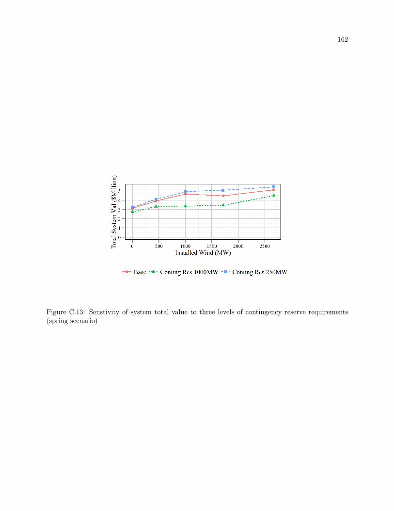
162

Figure C.13: Senstivity of system total value to three levels of contingency reserve requirements(spring scenario)

163

C.6 Summer Scenario with Spring Prices

Figure C.14 shows results from the summer Base case scenario and the same scenario run with

day-ahead energy market prices from the spring scenario to evaluate whether changes in system

behavior between the spring and summer scenarios are driven more by differences in hydrologic

and wind conditions or more by price differences. All other inputs are the same as for the base

summer scenario. Model outputs from the scenarios indicate that there is little difference in system

operations with the two price cases, only a shift of capacity away from the ancillary services market

to the energy market when the energy market prices are higher. The differences in total system

value are primarily due to the difference in ending energy in storage value which is based on the

energy prices. The physical ending storage is shown to be the same in both cases. Total hydro

generation and spill are nearly identical between the two cases. This reveals that the changes in

system behavior in the summer scenario, as they differ from the spring scenario, are primarily due

to the hydrologic and wind conditions and not the energy prices.

164

Figure C.14: Results from the summer scenario with energy prices from the spring scenario

165

C.7 Effects of Load Levels and Transmission Limits

Figure C.15 shows the expected outcome that the total system value (a) is higher when the

local load is lower (note that energy to meet local load is not given an explicit economic value in the

model). More capacity is available to sell in the market either as energy or ancillary services. The

net contribution of wind, however, shown by its average value per installed capacity (b) is greater

when the local load is higher and the additional generation is more necessary. When the local

load is low, more energy is sold from the hydropower system alone before adding wind generation;

therefore the added energy from wind is sold at a lower marginal price resulting in a lower net value.

The opposite is true in the high load case. The added wind energy is sold at a higher marginal

price.1 These results suggest there can be a large difference in the value of added wind generation

in different systems depending on how much energy they are already selling in the market and the

characteristics of the load they must meet.

Figure C.15: Spring scenarion load level effects on (a) Total System Value and (b) Average WindValue

1 It should be clarified here that we are not making a statement about which generating source has priority andshould receive a higher marginal price. The energy in our model is sold as a single quantity without distinction ofthe generating source. The use of terminology that suggests one generating source sells into the market first is onlyfor the purpose of explaining the results between the different load level scenarios.

166

When alternative transmission limits are combined with the load level cases (Figure C.16) it

is seen that increasing the transmission capacity from 1500 MW to 2500 MW has no effect for the

Base case. Transmission is not a constraining factor in the Base case. The added transmission only

has value when there is excess energy in the system. For the Low Load case the added transmission

provides added value at high wind penetrations in the spring scenario (a). The added transmission

allows more energy to be sold into the market as more wind generation is added. In the summer low

load scenario, the added value from increased transmission is only observed at low penetrations2

(b). Even at low penetrations there is excess energy in the system due to the high flows, and

the additional transmission allows for more of this energy to be sold into the market. At high

wind penetrations the reserve requirements become the constraining factor, not transmission, and

thus there is no added value from increased transmission. Results from the load and transmission

combinations suggest that it is not the sensitivity to a single parameter in isolation that is significant

but rather a combination of factors in the system. Here there is no sensitivity to added transmission

for the Base case loads. There is only a sensitivity to transmission limits when other factors change

as well, such as load, hydrologic conditions or wind.

2 Runs for the summer 40% wind case with low load and a 1500 MW transmission limit encountered infeasibilityissues when trying to accomodate high levels of wind and did not run to completion. For this reason, there is no datapoint at 40% wind in the Low Load 1500 case.

167

Figure C.16: Transmission and load combinations for the (a) spring and (b) summer scenarios andtheir effects on Total System Value

168

C.8 Market Depth Effects

Market depth influences total system value. In the Base case, the day-ahead energy market

clearing price is assumed to decrease 1% with each additional 50 MWh of energy sold into the

market. The Low Market Depth case increases this to 2%. For the Unlimited Market Depth case,

the price at a given hour does not change regardless of the amount of energy. The total system value

changes with market depth as expected as seen in Figure C.17(a), but the total hydro generation

(b) is nearly identical for all three cases suggesting there is little change in operational behavior

and the change in total value is simply due to the change in prices. There is an observed shift

in capacity away from ancillary services to energy when energy prices are higher in the Unlimited

Depth case and the opposite shift toward ancillary services when the energy prices are lower (c).

Figure C.17: Spring scenario market depth effects on (a) Total System Value, (b) Hydro Generationand (c) Ancillary Services Value

C.9 Effects of Wind Timing and Correlation with Prices

A description of the impacts on the integrated system when the timing of wind generation

is shifted is given in Section 4.5.3. The wind in this system is generally in phase with peak load

169

and price patterns. Figure C.18 shows that shifting the timing of wind generation back 6, 12 and

18 hours reduces the total system value (a) compared to the Base case even though there is little

change in total hydro generation (b). The reduction in value is due to the added wind generation

no longer matching peak pricing when the timing is shifted.

Figure C.18: Effects of shifting wind timing on (a) Total System Value and (b) Total HydroGeneration for the spring scenario