A Methodology to Assess Data Variability and Risk in a Pavement Design System for Bangladesh
206
UNIVERSITY OF BIRMINGHAM A METHODOLOGY TO ASSESS DATA VARIABILITY AND RISK IN A PAVEMENT DESIGN SYSTEM FOR BANGLADESH by MOHAMMED ZIAUL HAIDER A Thesis submitted to the University of Birmingham for the degree of MASTER OF PHILOSOPHY School of Civil Engineering College of Engineering and Physical Science University of Birmingham August 2009
Transcript of A Methodology to Assess Data Variability and Risk in a Pavement Design System for Bangladesh
UNIVERSITY OF BIRMINGHAM
A METHODOLOGY TO ASSESS DATA VARIABILITY AND RISK IN
A PAVEMENT DESIGN SYSTEM FOR BANGLADESH
by
MOHAMMED ZIAUL HAIDER
A Thesis submitted to
the University of Birmingham
for the degree of
MASTER OF PHILOSOPHY
School of Civil Engineering
College of Engineering and Physical Science
University of Birmingham
August 2009

University of Birmingham Research Archive
e-theses repository This unpublished thesis/dissertation is copyright of the author and/or third parties. The intellectual property rights of the author or third parties in respect of this work are as defined by The Copyright Designs and Patents Act 1988 or as modified by any successor legislation. Any use made of information contained in this thesis/dissertation must be in accordance with that legislation and must be properly acknowledged. Further distribution or reproduction in any format is prohibited without the permission of the copyright holder.
Abstract
This study aimed to develop a generic methodology to quantify the risk and reliability of
pavement and embankment design for Bangladesh considering the variability in design
data. The study also aimed to develop a construction quality control procedure to reduce the
variability in data.
To achieve this aim, data were collected from field and laboratory testing from four of the
country’s representative roads and a database was developed. The collected data were
studied and their variability was quantified. To develop a suitable risk quantification
methodology for Bangladesh, the existing methods were investigated and compared for
their appropriateness in connection with the proposed analytical pavement design method
and the prevailing conditions. The method proposed in this research utilizes the first order
second moment theory and an analytical model based on the method of equivalent
thickness. For the risk analysis of embankments the first order second moment method was
also identified as suitable in the context. An integrated example of the proposed procedure
is given, using the data from one of the roads tested. Existing quality control methods and
techniques were also reviewed to develop a suitable quality control procedure for
Bangladesh. For pavements, a performance based quality control procedure considering
their load carrying capacity as an acceptance criterion was also suggested in this research,
together with a quality control procedure for embankments.

THIS WORK IS DEDICATED TO MY PARENTS
Late Md. Rezaul Karim and
Mrs. Shamsun Nahar Begum

Acknowledgements
The author would like to express his sincere gratitude to his supervisor Dr. Harry T.
Evdorides for his intensive supervision, intellectual guidance, constructive criticism,
invaluable suggestions and monitoring through out the study.
The author also likes to express his special thanks to his co-supervisor Dr. M. P. N. Burrow
for his keen interest, valuable advice and comments during the research.
This study is a part of Bangladesh Road Pavement Research Project funded by the
Department for International Development (DFID). The author is indebted to Professor M.
S. Snaith (Chairman of steering committee), Dr. Gurmel S. Ghataora (Co-investigator), and
A. R. M. Anwar Hossain (former Chief Engineer of Roads and Highways Department of
Bangladesh) for their respective contribution in the research project.
The author is grateful to the Roads and Highways Department of Bangladesh for giving
him the opportunity to conduct the research and the Department for International
Development (DFID) for sponsoring the research project.
The author is also grateful to his wife and child for their sacrifice during the study.
Last but not least, the author would like to give his most sincere thanks to his mother for
her never-ending support and encouragement.
TABLE OF CONTENTS CHAPTER 1 INTRODUCTION ...............................................................................................1
1.1 BACKGROUND ....................................................................................................................... 1 1.2 PROBLEM DEFINITION............................................................................................................ 1 1.3 AIMS AND OBJECTIVES OF THE STUDY.................................................................................. 2 1.4 BENEFITS OF THE STUDY ....................................................................................................... 2 1.5 LAYOUT OF THE THESIS ........................................................................................................ 3
CHAPTER 2 LITERATURE REVIEW ...................................................................................5
2.1 INTRODUCTION...................................................................................................................... 5 2.2 PAVEMENT DESIGN PROCEDURES AND REQUIRED DATA....................................................... 5
2.2.1 Generic design ............................................................................................................... 5 2.2.2 Empirical design............................................................................................................ 6 2.2.3 Analytical design ........................................................................................................... 7
2.2.3.1 Pavement design data ............................................................................................. 9 2.3 EMBANKMENT DESIGN PROCEDURES AND REQUIRED DATA ............................................... 10
2.3.1 Generic embankment design........................................................................................ 10 2.3.2 Embankment design data ............................................................................................. 11
2.4 VARIABILITY OF MATERIALS AND DATA ............................................................................. 12 2.4.1 Pavement data ............................................................................................................. 12
2.4.1.1 Traffic................................................................................................................... 12 2.4.1.2 Materials............................................................................................................... 12 2.4.1.3 Construction ......................................................................................................... 13
2.4.2 Embankment data ........................................................................................................ 13 2.5 DATA VARIABILITY QUANTIFICATION METHODS ................................................................ 14 2.6 RISK ANALYSIS METHODS ................................................................................................... 15 2.7 DEVELOPED METHODS FOR PAVEMENT RISK ANALYSIS...................................................... 17
2.7.1 Austroads [2004] ......................................................................................................... 17 2.7.2 AASHTO [1993] .......................................................................................................... 18
2.7.2.1 Noureldin et al. [1994, 1996] ............................................................................... 19 2.7.2.2 Huang [1993]........................................................................................................ 20
2.7.3 NCHRP [2004] ............................................................................................................ 20 2.7.4 Kim [2006]................................................................................................................... 20 2.7.5 TRRL [1975]................................................................................................................ 21 2.7.6 Chua et al. [1992]........................................................................................................ 21 2.7.7 Alsherri and George [1988] ........................................................................................ 22 2.7.8 Kulkarni [1994] ........................................................................................................... 23 2.7.9 Zhang [2006] ............................................................................................................... 23 2.7.10 Lua et al. [1996] ........................................................................................................ 24 2.7.11 Brown [1994]............................................................................................................. 24
2.8 DEVELOPED METHODS FOR EMBANKMENT RISK ANALYSIS ................................................ 25 2.8.1 Developed methods of slope stability risk analysis...................................................... 25
2.8.1.1 First-order second moment method...................................................................... 26 2.8.1.2 Point estimation method....................................................................................... 27 2.8.1.3 Monte Carlo simulation........................................................................................ 27 2.8.1.4 Mean first order reliability method....................................................................... 28 2.8.1.5 Risk analysis algorithm with Fellenius limit equilibrium method........................ 28
i
2.8.1.6 Deterministic approach using fuzzy set................................................................ 29 2.8.1.7 Random finite element method ............................................................................ 30 2.8.1.8 Finite-element method with the first-order reliability method ............................. 30
2.8.2 Developed methods of settlement risk analysis............................................................ 30 2.8.2.1 Fenton and Griffiths [2002].................................................................................. 30
2.9 QUALITY CONTROL AND QUALITY ASSURANCE .................................................................. 31 2.10 SUMMARY.......................................................................................................................... 33
CHAPTER 3 RESEARCH METHODOLOGY .....................................................................34
3.1 INTRODUCTION.................................................................................................................... 34 3.2 OVERALL APPROACH........................................................................................................... 34 3.3 DATABASE DEVELOPMENT.................................................................................................. 35 3.4 PAVEMENT DESIGN DATA VARIABILITY ANALYSIS ............................................................. 35
3.4.1 Traffic prediction variation analysis ........................................................................... 35 3.4.1.1 Variation in average daily traffic in heavier direction.......................................... 35 3.4.1.2 Axle load composition.......................................................................................... 36 3.4.1.3 Variation in percent of trucks in design lane........................................................ 36
3.4.2 Pavement performance prediction uncertainties analysis ........................................... 37 3.4.2.1 Variation in pavement layer thickness ................................................................. 37 3.4.2.2 Variation in pavement layer strength ................................................................... 37 3.4.2.3 Sub-grade stiffness variation ................................................................................ 37
3.5 EMBANKMENT DESIGN DATA VARIABILITY ANALYSIS........................................................ 38 3.6 DESIGN RISK QUANTIFICATION AND RELIABILITY INTEGRATION........................................ 38 3.7 OVERALL RISK AND RELIABILITY........................................................................................ 39 3.8 QUALITY CONTROL AND QUALITY ASSURANCE .................................................................. 39 3.9 SUMMARY............................................................................................................................ 40
CHAPTER 4 DATA QUALITY ANALYSIS .........................................................................41
4.1 INTRODUCTION.................................................................................................................... 41 4.2 DATA COLLECTION ............................................................................................................. 41 4.3 PAVEMENT DATA QUALITY ANALYSIS ............................................................................... 42
4.3.1 Traffic prediction data ................................................................................................. 42 4.3.1.1 Traffic data ........................................................................................................... 42 4.3.1.2 Axle load data....................................................................................................... 44
4.3.2 Deflection data............................................................................................................. 45 4.3.3 Pavement layer thickness data..................................................................................... 48 4.3.4 Variation in pavement layer strength data .................................................................. 52 4.3.5 Pavement Roughness data variation............................................................................ 57
4.4 EMBANKMENT DATA QUALITY ANALYSIS ......................................................................... 59 4.4.1 Index Properties........................................................................................................... 59 4.4.2 Shear strength data...................................................................................................... 63 4.4.3 Consolidation data....................................................................................................... 64
4.5 SUMMARY............................................................................................................................ 68
CHAPTER 5 PAVEMENT DESIGN RISK AND RELIABILITY ......................................69
5.1 INTRODUCTION.................................................................................................................... 69 5.2 ASSESSMENT OF THE AVAILABLE METHODS ....................................................................... 69 5.3 PROPOSED APPROACH......................................................................................................... 72
5.3.1 Development of the proposed method.......................................................................... 72 5.3.2 Detailed description of the proposed method of analysing pavement design risk....... 73 5.3.3 Proposed alternative approach of analysing pavement design risk (FOSM).............. 75
ii
5.4 SUMMARY............................................................................................................................ 77
CHAPTER 6 EMBANKMENT DESIGN RISK AND RELIABILITY ...............................78
6.1 INTRODUCTION.................................................................................................................... 78 6.2 EMBANKMENT SLOPE STABILITY RISK ANALYSIS ............................................................... 78
6.2.1 Assessment of the available methods ........................................................................... 78 6.2.2 Suggested Approach .................................................................................................... 81
6.3 EMBANKMENT SETTLEMENT RISK ANALYSIS ...................................................................... 84 6.3.1 Assessment of the available methods ........................................................................... 84 6.3.2 Proposed method ......................................................................................................... 85
6.4 EMBANKMENT RISK FOR BOTH SLOPE STABILITY AND SETTLEMENT.................................. 89 6.5 OVERALL RISK OF PAVEMENT-EMBANKMENT DESIGN SYSTEM .......................................... 89 6.6 SUMMARY............................................................................................................................ 90
CHAPTER 7 AN INTEGRATED EXAMPLE.......................................................................91
7.1 INTRODUCTION.................................................................................................................... 91 7.2 PAVEMENT DESIGN RISK QUANTIFICATION ......................................................................... 91
7.2.1 Application example of proposed method.................................................................... 91 7.2.2 Comparison of results with other methods .................................................................. 95
7.3 EMBANKMENT DESIGN RISK QUANTIFICATION ................................................................... 97 7.3.1 Quantification of embankment design risk against slope stability .............................. 97 7.3.2 Quantification of embankment design risk against settlement................................... 101 7.3.3 Quantification of embankment risk for both slope stability and settlement............... 108
7.4 OVERALL RISK QUANTIFICATION ...................................................................................... 108 7.5 SUMMARY.......................................................................................................................... 109
CHAPTER 8 PAVEMENT CONSTRUCTION QUALITY CONTROL ..........................110
8.1 INTRODUCTION.................................................................................................................. 110 8.2 DEVELOPED METHODS ...................................................................................................... 110
8.2.1 Quality control tests................................................................................................... 110 8.2.2 Quality measures and conformance .......................................................................... 111 8.2.3 Performance relationship .......................................................................................... 112 8.2.4 Pay adjustment........................................................................................................... 112
8.3 COMPARISON OF THE DEVELOPED METHODS AND TECHNIQUES ....................................... 114 8.4 LOGICAL DEVELOPMENT OF THE PROPOSED METHOD....................................................... 116 8.5 PROPOSED METHODS ........................................................................................................ 118
8.5.1 Performance based quality control............................................................................ 118 8.5.2 Step-by-step Quality Control ..................................................................................... 121
8.6 SUMMARY.......................................................................................................................... 124
CHAPTER 9 EMBANKMENT CONSTRUCTION QUALITY CONTROL ...................125
9.1 INTRODUCTION.................................................................................................................. 125 9.2 DEVELOPED METHODS...................................................................................................... 125
9.2.1 Quality control of embankment constructed with soft sedimentary rock................... 125 9.2.2 End-result based embankment construction quality control procedure .................... 126 9.2.3 AASHTO [1996] Guideline........................................................................................ 127
9.3 COMPARISON OF THE DEVELOPED METHODS .................................................................... 128 9.4 LOGICAL DEVELOPMENT OF THE PROPOSED METHOD....................................................... 129 9.5 DETAILED DESCRIPTION OF THE PROPOSED METHOD........................................................ 130 9.6 SUMMARY.......................................................................................................................... 133
iii
CHAPTER 10 AN EXAMPLE APPLYING THE QUALITY CONTROL PROCESS ....135
10.1 INTRODUCTION................................................................................................................ 135 10.2 APPLICATION EXAMPLE OF THE PROPOSED METHOD WITH FIELD DATA ......................... 135
10.2.1 Performance based quality control example ........................................................... 135 10.2.2 Step-by-step quality control example....................................................................... 138
10.3 SUMMARY........................................................................................................................ 142
CHAPTER 11 DISCUSSION .................................................................................................143
11.1 INTRODUCTION................................................................................................................ 143 11.2 VARIABILITY IN DESIGN DATA ........................................................................................ 144 11.3 QUANTIFICATION OF PAVEMENT DESIGN RISK ................................................................ 144 11.4 QUANTIFICATION OF EMBANKMENT DESIGN RISK .......................................................... 147 11.5 QUANTIFICATION OF OVERALL DESIGN RISK .................................................................. 148 11.6 QUALITY CONTROL PROCESS FOR PAVEMENT AND EMBANKMENT CONSTRUCTION ...... 149
11.6.1 Quality control system for pavement ....................................................................... 149 11.6.2 Quality control system for Embankments ................................................................ 150
11.7 APPLICABILITY OF THE PROPOSED PROCEDURE .............................................................. 150 11.8 RECOMMENDATIONS TO REDUCE THE RISK IN DESIGN AND PERFORMANCE................... 151 11.9 RECOMMENDATIONS FOR FURTHER RESEARCH .............................................................. 153 11.10 SUMMARY...................................................................................................................... 153
CHAPTER 12 CONCLUSIONS ............................................................................................155
REFERENCES ...........................................................................................................................159
APPENDIX A PROPOSED ALTERNATIVE METHOD EXAMPLE .............................173
APPENDIX B NOURELDIN ET AL. [1994] METHOD EXAMPLE................................178
APPENDIX C CHARTS FOR ESTIMATING LAYER CO-EFFICIENT........................182
APPENDIX D DEFINITION OF DIFFERENT TYPES OF VEHICLE...........................186
APPENDIX E STATISTICAL TABLES ..............................................................................187
APPENDIX F OTHER TABLES AND GRAPHS ...............................................................191
iv
List of Figures
Figure 2.1: A Generic Pavement Design Flowchart …………….………………………..6
Figure 2.2: Analytical Pavement Design Method Flowchart …………………………......8
Figure 2.3: A Generic Embankment Design Flowchart………………………………….11
Figure 3.1: Research Methodology Flowchart………………………………………..….34
Figure 4.1: Composition of traffic in Road N4 ...………………………………………..42
Figure 4.2: Composition of traffic in Road N302 ……….………….…………………...43
Figure 4.3: Composition of traffic in Road R301……………………………………......43
Figure 4.4: Composition of traffic in Road Z3024 ……………………………………...43
Figure 4.5: Variation of deflection data in Road N4 ………………………………...….46
Figure 4.6: Variation of deflection data in Road N302…………………………….…....46
Figure 4.7: Variation of deflection data in Road R301…………………………………..47
Figure 4.8: Variation of deflection data in Road Z3024………………………..….….…47
Figure 4.9: Variation in pavement layer thickness in Road N4………………….………48
Figure 4.10: Variation in pavement layer thickness in Road N302……………….……..49
Figure 4.11: Variation in pavement layer thickness in Road R301……………….….….49
Figure 4.12: Variation in pavement layer thickness in Road Z3024………………….....50
Figure 4.13: Variation in CBR estimated from DCP tests in Road N4………………….52
Figure 4.14: Variation in CBR estimated from DCP tests in Road N302…………….…52
Figure 4.15: Variation in CBR estimated from DCP tests in Road R301…………….….53
Figure 4.16: Variation in CBR estimated from DCP tests in Road Z3024……….….…..53
Figure 4.17: Variation in soaked CBR in Road N4…………………………………...…54
Figure 4.18: Variation in soaked CBR in Road N302……………………………..….…55
Figure 4.19: Variation in soaked CBR in Road R301…………………………………...55
Figure 4.20: Variation in soaked CBR in Road Z3024………………………….………55
Figure 4.21: Variation in roughness (IRI) data in Road N4…………………….……….57
Figure 4.22: Variation in roughness (IRI) data in Road N302…………………………..57
Figure 4.23: Variation in roughness (IRI) data in Road R301………………….…….….58
Figure 4.24: Variation in roughness (IRI) data in Road Z3024…………….………...….58
Figure 4.25: Variation in liquid limit at different depths ………………………………..60
v
Figure 4.26: Variation in plastic limit at different depths…………….……….….……...60
Figure 4.27: Variation in plasticity index at different depths…………………………....60
Figure 4.28: Variation in moisture content at different depths……………….……….....61
Figure 4.29: Variation in unit weight at different depths…………………………..….…61
Figure 4.30: Variation in dry unit weight at different depths………………………........61
Figure 4.31: Variation in specific gravity at different depths………………….….….….62
Figure 4.32: Variation in initial void ratio at different depths………………………...…62
Figure 4.33: Variation in soil cohesion………………………………………….…….....63
Figure 4.34: Variation in soil angle of internal friction……………………………….....63
Figure 4.35: Variation in soil undrained modulus………………………………….……65
Figure 4.36: Variation in initial void ratio (remoulded soil) ……………………..….….65
Figure 4.37: Variation in soil dry density ………………………………….……………66
Figure 4.38: Variation in soil saturated density…………………………….……………66
Figure 4.39: Variation in soil compression index….……………………….……………67
Figure 4.40: Variation in soil secondary compression index………………….…………67
Figure 5.1: Risk analysis flowchart of the proposed first procedure………………….....73
Figure 5.2: Flowchart of the proposed alternative risk analysis procedure ……………..76
Figure 6.1: Proposed embankment slope stability risk analysis flowchart ………..…….82
Figure 6.2: Proposed embankment settlement risk analysis flowchart……………......…86
Figure 8.1: Performance based quality control flowchart……………………………....119
Figure 8.2: Flowchart for Step-by-step quality control in pavement construction…......122
Figure 9.1: Embankment Construction Quality Control Flowchart ……………………131
Figure 11.1: Variation of reliability design factor with design reliability level…….….146
Figure 11.2: Survey results for reason of difficulty in achieving quality ………….…..152
vi
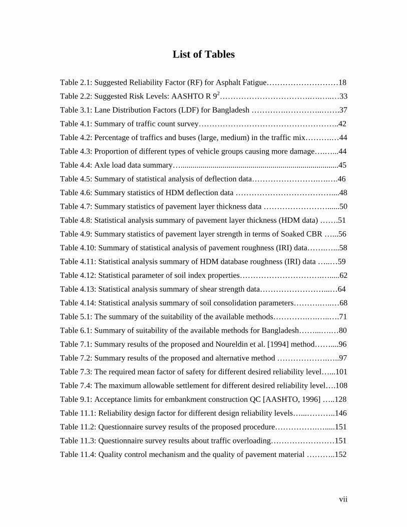
List of Tables
Table 2.1: Suggested Reliability Factor (RF) for Asphalt Fatigue………………………18
Table 2.2: Suggested Risk Levels: AASHTO R 92…………………………….….…..…33
Table 3.1: Lane Distribution Factors (LDF) for Bangladesh ………….…………..…….37
Table 4.1: Summary of traffic count survey……………………………………………..42
Table 4.2: Percentage of traffics and buses (large, medium) in the traffic mix……….…44
Table 4.3: Proportion of different types of vehicle groups causing more damage….…...44
Table 4.4: Axle load data summary…...............................................................................45
Table 4.5: Summary of statistical analysis of deflection data…………………….….….46
Table 4.6: Summary statistics of HDM deflection data ………………………………....48
Table 4.7: Summary statistics of pavement layer thickness data ……………………......50
Table 4.8: Statistical analysis summary of pavement layer thickness (HDM data) …….51
Table 4.9: Summary statistics of pavement layer strength in terms of Soaked CBR …...56
Table 4.10: Summary of statistical analysis of pavement roughness (IRI) data…….…...58
Table 4.11: Statistical analysis summary of HDM database roughness (IRI) data …..…59
Table 4.12: Statistical parameter of soil index properties………………………….….....62
Table 4.13: Statistical analysis summary of shear strength data……………………...…64
Table 4.14: Statistical analysis summary of soil consolidation parameters……….…..…68
Table 5.1: The summary of the suitability of the available methods………….….…..….71
Table 6.1: Summary of suitability of the available methods for Bangladesh……...….…80
Table 7.1: Summary results of the proposed and Noureldin et al. [1994] method……....96
Table 7.2: Summary results of the proposed and alternative method ……………….…..97
Table 7.3: The required mean factor of safety for different desired reliability level…...101
Table 7.4: The maximum allowable settlement for different desired reliability level….108
Table 9.1: Acceptance limits for embankment construction QC [AASHTO, 1996] …..128
Table 11.1: Reliability design factor for different design reliability levels…...………..146
Table 11.2: Questionnaire survey results of the proposed procedure…………….….....151
Table 11.3: Questionnaire survey results about traffic overloading……………………151
Table 11.4: Quality control mechanism and the quality of pavement material ………..152
vii

Glossary of Symbols and Non-standard Abbreviations
A Axles per Truck
AADT Annual Average Daily Traffic
AADTT Annual Average Daily Truck Traffic
AASHTO American Association of State Highway and Transportation Officials
AC Asphaltic Concrete
c´ Drained Cohesion
Cc Compression Index
Cα Secondary Compression Index
CBR California Bearing Ratio
COV Co-efficient of Variation
D Directional Distribution
DCP Dynamic Cone Penetrometer
e0 Initial Void Ratio
ep Void Ratio at the End of Primary Consolidation
EALF Equivalent Axle Load Factor
ESAL Equivalent Standard Axle Loads
f Strength Reduction Ratio
F Factor of Safety
FR Reliability Design Factor
Fi Equivalent Axle Load Factor for the ith Load Group
FEM Finite Element Method
FOSM First Order Second Moment
FWD Falling Weight Deflectometer
G Growth Factor
GPR Ground Penetrating Radar
H Layer Thickness
HDM Highway Design and Management
L Lane Distribution
MET Method of Equivalent Thickness
viii
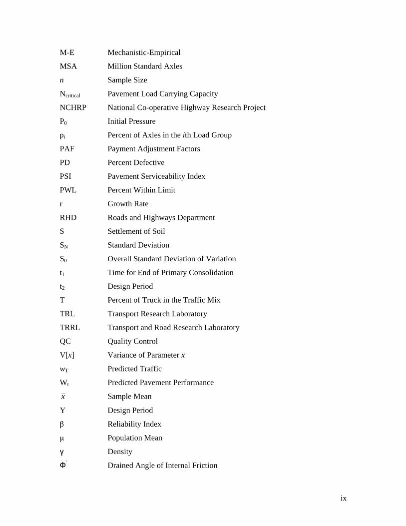
M-E Mechanistic-Empirical
MSA Million Standard Axles
n Sample Size
Ncritical Pavement Load Carrying Capacity
NCHRP National Co-operative Highway Research Project
P0 Initial Pressure
pi Percent of Axles in the ith Load Group
PAF Payment Adjustment Factors
PD Percent Defective
PSI Pavement Serviceability Index
PWL Percent Within Limit
r Growth Rate
RHD Roads and Highways Department
S Settlement of Soil
SN Standard Deviation
S0 Overall Standard Deviation of Variation
t1 Time for End of Primary Consolidation
t2 Design Period
T Percent of Truck in the Traffic Mix
TRL Transport Research Laboratory
TRRL Transport and Road Research Laboratory
QC Quality Control
V[x] Variance of Parameter x
wT Predicted Traffic
Wt Predicted Pavement Performance
x Sample Mean
Y Design Period
β Reliability Index
μ Population Mean
γ Density
Ф´ Drained Angle of Internal Friction
ix
Chapter 1 Introduction
1.1 Background
The research reported in this thesis is part of a major research programme which sought
to develop a methodology for pavement design suitable for Bangladesh. It focuses on an
examination of the variability of data associated with pavement and embankment design
and suggests methods to quantify and control it in both the design and construction
phases.
The principal goal of any engineering design process is to produce a system which
performs its intended function in a clear, swift and accurate manner. But the success of
any design method depends on the accurate characterization of the uncertainties in
preparing the design inputs. The design of pavements involves a number of input data.
Consequently, the quality of these input data has significant effects on the design of the
pavement. To address this problem, the concepts of reliability and probability were
employed first in the early 1970s by researchers and engineers such as Lemer and
Noavenzadeh [1971] and Kher and Darter [1973]. A number of items may contribute to
the reliability of the design and the variability of data. In Bangladesh such items include
overloading [Khan, 2005], poor construction practices and seasonal variation in the
moisture content of granular materials and subgrade soil. Hence, for the methodology of
new pavement design it was felt necessary for Bangladesh, where road pavements are
usually built on embankments, to incorporate the concept of reliability. Their satisfactory
performance depends on the performance of the embankment. Therefore the quality of
embankment design data also needed to be considered in the country’s proposed design
system, together with a quality control process to reduce the variability of pavement
properties during construction.
1.2 Problem definition
The design of a highway pavement and embankment in Bangladesh should consider the
variability of the input data. This variability may influence the success of the pavement
and embankment design and consequently can lead to premature failure. To date, no
study has been conducted in Bangladesh to assess such variability in design data and its
1

effects on the design. The assessment of variation in design data necessitates a thorough
investigation of the design data collected from field and laboratory tests of representative
roads. A methodology is also required for designers to quantify the variability in design
data and its impact on the design produced, so that the reliability of the overall design can
be determined. Moreover, a system of quality control and assurance associated with the
design system is also required to reduce the variability of the construction related data.
There are some methods of quantifying design risk associated with data variability
available in the literature. But these were developed for particular conditions or are
considered unique design models and may not be suitable for Bangladesh. Hence, an
amended methodology is required which is suitable for the country’s geographical,
geotechnical and socio-economic conditions.
1.3 Aims and Objectives of the study
The aim of this study is to develop a methodology to assess the variability of data and
associated risk in a pavement design system for Bangladesh. To achieve this aim, the
following objectives have been set up for the study:
1. To assess the variability of the pavement and embankment design data
2. To develop a methodology which will quantify the variability of data
3. To quantify the risk and reliability in the pavement and embankment design system
4. To introduce a quality control and assurance process in the design system, based
on the data considered by the design system.
1.4 Benefits of the study
The main beneficiary of this study will be the Roads and Highways Department (RHD)
of Bangladesh, which is responsible for the design, construction and maintenance of the
major road network there. The research output will help RHD in improving the quality of
the design data, incorporating the desired level of reliability in designing and ultimately
in obtaining a satisfactory performance from pavements and embankments. Other
engineering departments which deal with the local road network of Bangladesh will also
benefit from this study if they incorporate the research finding in their design system.
Ultimately, the road agencies of similar developing countries may benefit from this
research.
2
1.5 Layout of the Thesis
To achieve the above objectives this Thesis is structured as follows:
Chapter 2 presents a literature review of methods of pavement and embankment design,
design data, data variability, methods of determining data variability, quantifying risk
and quality control.
Chapter 3 describes the methodology followed in the present study to examine the
variability of design parameters and the factors and techniques used for risk
quantification and quality control.
Chapter 4 describes the quality and variability in the design data collected from field and
laboratory testing carried out on four representative roads of Bangladesh.
Chapter 5 investigates the suitability of existing methods of analysing pavement design
risk for the design system of Bangladesh and provides a comparative study of them.
Then it discusses the logical development of the proposed method, together with a
detailed description of the proposed method.
Chapter 6 presents the development of a risk quantification process for embankment
design system of Bangladesh. It reviews the existing methods of risk analysis with
regard to slope stability and settlement and presents a method which has been
developed. The methodology intended to quantify the overall risk of this pavement-
embankment design system is also presented.
Chapter 7 presents an integrated example of the proposed procedure, calculating the
overall design risk using the data collected from a road of Bangladesh.
Chapter 8 deals with the development of a quality control process for pavement
construction of Bangladesh. Then the development of the proposed performance based
quality control system is described. A step-by-step quality control process during
construction is also given.
Chapter 9 investigates the existing state of knowledge for embankment construction
quality control. A comparative study of them is also provided. The Chapter then
describes the quality control process for embankment construction of Bangladesh.
Chapter 10 gives an application example of the quality control process which is being
proposed for Bangladesh with the field collected data.
3

Chapter 11 discusses the key findings of the study. It investigates the suitability of the
proposed procedures through an analysis of the opinion of the RHD road engineers. It
also recommends some ways of reducing risk in design and performance and specifies
some areas for further research.
Chapter 12 draws some conclusions from the study.
4

Chapter 2 Literature Review
2.1 Introduction
This chapter reviews the process of pavement and embankment design and its associated
design data, the variability in the data and the associated risk, the variability resulting
from poor construction and the fundamentals of the quality control process. In more
detail, this chapter first describes pavement design, in particular, analytical pavement
design and its associated input parameters. It goes on to discuss the processes of
embankment design in the light of slope stability and settlement and identifies the
associated design input parameters. Subsequently, it reviews the methods used to
quantify the variability associated with the data of pavement and embankment design and
discusses the methods used to quantify risk. However, a detailed review of the existing
risk quantification methods for their problems and appropriateness to Bangladesh are
provided in Chapter 5 and Chapter 6 for pavement and embankment respectively. Before
concluding, this chapter considers quality control systems.
2.2 Pavement design procedures and required data
There are two main types of pavement, flexible and rigid. Only the design procedures of
flexible pavement will be considered in this chapter, since Bangladesh has no rigid
pavements.
2.2.1 Generic design
The main goal of a flexible pavement design is to provide a structure that can carry the
anticipated traffic, withstand the environmental effects and maintain a satisfactory level
of service for a predefined period of time. A flexible pavement is usually designed as a
system of a layered structure. The designer should consider using the locally available
materials and should select the most economical combination of layer thickness and
materials that performs the intended function satisfactorily. A cost analysis of pavement
life cycle may be performed to evaluate the most economical option for pavement design.
A design system in general requires the input of information on cumulative traffic that it
is anticipated the pavement must carry in its projected life, the properties of the materials
5
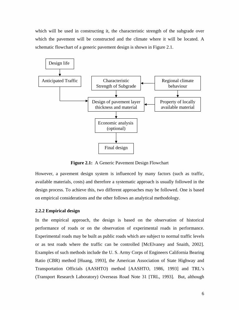
which will be used in constructing it, the characteristic strength of the subgrade over
which the pavement will be constructed and the climate where it will be located. A
schematic flowchart of a generic pavement design is shown in Figure 2.1.
Anticipated Traffic Characteristic Strength of Subgrade
Regional climate behaviour
Design of pavement layer thickness and material
Economic analysis (optional)
Property of locally available material
Final design
Design life
Figure 2.1: A Generic Pavement Design Flowchart
However, a pavement design system is influenced by many factors (such as traffic,
available materials, costs) and therefore a systematic approach is usually followed in the
design process. To achieve this, two different approaches may be followed. One is based
on empirical considerations and the other follows an analytical methodology.
2.2.2 Empirical design
In the empirical approach, the design is based on the observation of historical
performance of roads or on the observation of experimental roads in performance.
Experimental roads may be built as public roads which are subject to normal traffic levels
or as test roads where the traffic can be controlled [McElvaney and Snaith, 2002].
Examples of such methods include the U. S. Army Corps of Engineers California Bearing
Ratio (CBR) method [Huang, 1993], the American Association of State Highway and
Transportation Officials (AASHTO) method [AASHTO, 1986, 1993] and TRL’s
(Transport Research Laboratory) Overseas Road Note 31 [TRL, 1993]. But, although
6
empirical pavement design methods have been popular in the past, it is difficult to use
them accurately when the design input factors differ significantly from those used in the
original design. These factors may include changes in traffic levels, climatic factors and
the availability of materials. Consequently, empirical methods are ineligible in the
present context and will not be discussed further.
2.2.3 Analytical design
In the analytical approach, the design is based on the structural analysis of pavements and
their predicted performance in relation to measurable parameters. A significant number of
analytical pavement design methods is described in the literature and commonly used
ones include those developed by Shell International Petroleum Ltd [Shell 1978], the
Asphalt Institute [1981]; Austroads [2004] and Nottingham University [Brunton et al.
1987]. This approach to pavement design is becoming more popular with advances in
computer hardware and software technologies. As a result, many countries all over the
world have partially or fully implemented analytical procedures for determining the
existing strength (bearing capacity) of road pavements, for analyzing and designing new
roads and for rehabilitating existing road pavements.
In analytical pavement design, two models are used. One is associated with the pavement
response under traffic loads and the other concerns pavement performance. For the
former, a structural model of the pavement is built and used to determine stresses, strains
and deflections at critical locations in the pavement. The parameters determined at those
locations are known as critical response parameters. The performance model, on the
other hand, is used to estimate pavement life as a function of the critical response
parameters.
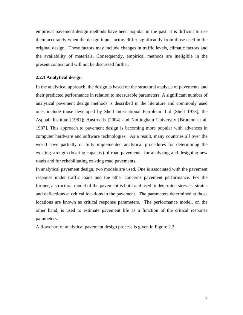
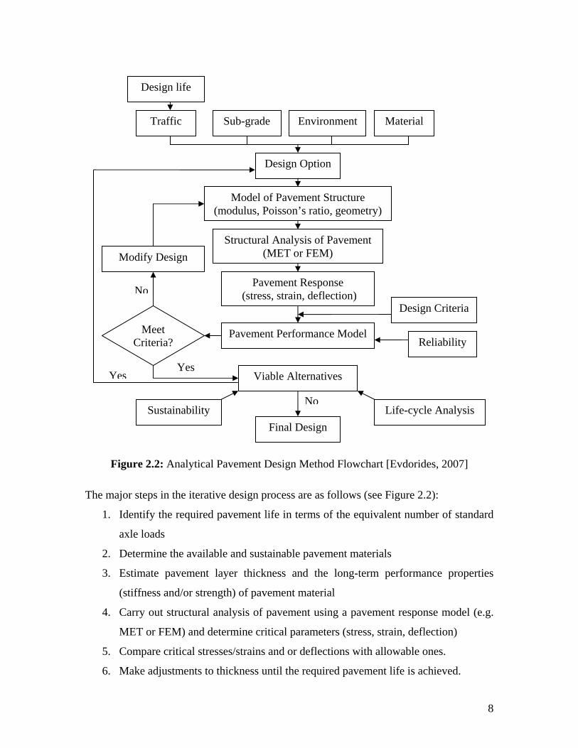
A flowchart of analytical pavement design process is given in Figure 2.2.
7
Traffic Environment Material
Reliability
Pavement Response (stress, strain, deflection)
Structural Analysis of Pavement (MET or FEM)
Model of Pavement Structure (modulus, Poisson’s ratio, geometry)
Design Option
Pavement Performance Model
Life-cycle Analysis
Modify Design
Viable Alternatives
Design Criteria
Final Design Sustainability
Meet Criteria?
Sub-grade
Yes Yes
No
No
Design life
Figure 2.2: Analytical Pavement Design Method Flowchart [Evdorides, 2007]
The major steps in the iterative design process are as follows (see Figure 2.2):
1. Identify the required pavement life in terms of the equivalent number of standard
axle loads
2. Determine the available and sustainable pavement materials
3. Estimate pavement layer thickness and the long-term performance properties
(stiffness and/or strength) of pavement material
4. Carry out structural analysis of pavement using a pavement response model (e.g.
MET or FEM) and determine critical parameters (stress, strain, deflection)
5. Compare critical stresses/strains and or deflections with allowable ones.
6. Make adjustments to thickness until the required pavement life is achieved.
8
2.2.3.1 Pavement design data
Traffic data are important as inputs for the analysis and design of pavement structures,
because they are used to determine the loading regime to which the structure will be
subject throughout its design life. Most existing design procedures, including all of the
AASHTO (American Association of State Highway and Transportation Officials) Design
Guides, quantify traffic in terms of equivalent standard axle loads (ESALs) [Schwartz,
2007]. This enables a single load to be used as a unit for design purposes and requires all
other traffic loads to be converted to this design load. However, the mechanistic
pavement response models in the Mechanistic-Empirical (M-E) pavement design guide
require the magnitudes and frequencies to be specified of the actual wheel loads which
the pavement is expected to bear throughout its design life. According to this guide,
traffic must be specified in terms of axle load spectra rather than ESALs. Axle load
spectra are the frequency distributions of axle load magnitudes by axle type (single,
tandem, tridem, quad) and season (typically, per month) [Papagiannakis et al., 2006].
The traffic related information required by a standard design process includes the
following [Killingsworth and Zollinger, 1995]:
• Traffic volume—base year information
- Two-way annual average daily truck traffic (AADTT)
- Number of lanes in the design direction
- Percentage of trucks in the design direction
- Percentage of trucks in the design lane
- Vehicle (truck) operational speed
• Traffic volume adjustment factors
- Seasonal variation / adjustment
- Vehicle class distribution
- Hourly truck distribution
- Traffic growth factors
• Axle load distribution factors by season, vehicle class and axle type (single,
tandem, tridem and quadruple axles)
• General traffic inputs
- Number of axles/trucks
9

- Axle configuration (axle width and spacing; tyre spacing and pressure)
- Wheelbase spacing distribution
Another important input parameter for pavement design is the properties of the material
to be used in the pavement layers. The information of resilient modulus and Poisson’s
ratio of different pavement layers is required in the mechanistic analysis of pavement
structure. The resilient modulus and Poisson’s ratio of subgrade soil are also required for
the design of pavement structure.
In obtaining the reliable input data required for design, a major difficulty is that the
required site specific information is not generally available at the design stage and
sometimes has to be estimated several years in advance of construction. Further, the
actual properties of the material to be used are not usually known much before
construction takes place. Nevertheless, a designer should obtain as much information as
possible on in-situ material properties, traffic and other inputs in order to supply a
realistic design. To this end, the designer should undertake a sensitivity analysis to
identify the most important factors to affect the design [Castell and Pintado, 1999;
Killingsworth and Zollinger, 1995].
2.3 Embankment design procedures and required data
An embankment is designed for various purposes, such as to sustain other civil
engineering structures (highways, railways) and to restrain water (dams). Only the
general design procedures of highway embankments will be discussed in this chapter.
2.3.1 Generic embankment design
Highway embankments are important and costly civil engineering structures which
provide an essential platform for pavements. The critical aspects of embankment design
are the analysis of stability and settlement for safety of the earth structure under various
operating and environmental conditions. The prime concern should be to select an
economical design using locally available material and technology, so that the
embankment can perform its intended function satisfactorily. A highway embankment is
considered to be performing satisfactorily when it can carry the load borne by the road
pavement and the environment while maintaining its stability and settlement to a
tolerable limit during its service life. An embankment design system in general requires,
10
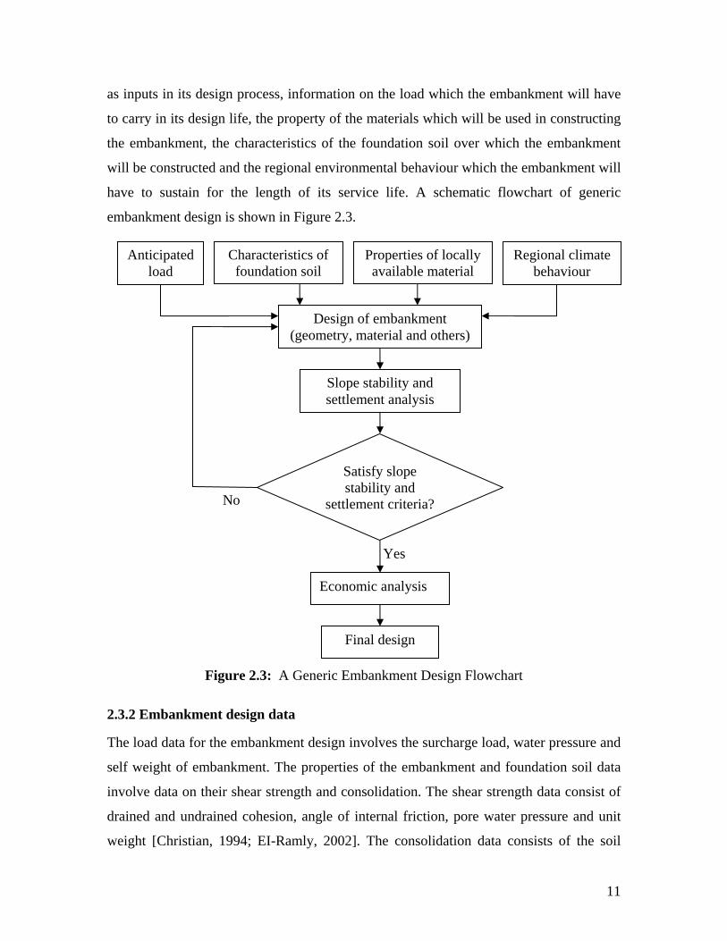
as inputs in its design process, information on the load which the embankment will have
to carry in its design life, the property of the materials which will be used in constructing
the embankment, the characteristics of the foundation soil over which the embankment
will be constructed and the regional environmental behaviour which the embankment will
have to sustain for the length of its service life. A schematic flowchart of generic
embankment design is shown in Figure 2.3.
Design of embankment (geometry, material and others)
Economic analysis
No
Slope stability and settlement analysis
Regional climate behaviour
Yes
Satisfy slope stability and
settlement criteria?
Properties of locally available material
Characteristics of foundation soil
Anticipated load
Final design
Figure 2.3: A Generic Embankment Design Flowchart
2.3.2 Embankment design data
The load data for the embankment design involves the surcharge load, water pressure and
self weight of embankment. The properties of the embankment and foundation soil data
involve data on their shear strength and consolidation. The shear strength data consist of
drained and undrained cohesion, angle of internal friction, pore water pressure and unit
weight [Christian, 1994; EI-Ramly, 2002]. The consolidation data consists of the soil
11
modulus, Poisson’s ratio, initial void ratio, density, compression index, secondary
compression index, time for end of primary consolidation, design period and layer
thickness of the different layers [Craig, 2004; Das, 1997; Tomlinson, 2001; Barnes,
1995]. The environmental data involve the amount of rainfall and water table height, etc.
It is very difficult to obtain accurate information about these parameters in designing an
embankment, since soil properties vary from one location to another and the
environmental behaviour is also variable. However, to obtain an optimal design, as much
information as possible should be collected by conducting a thorough site investigation
and by testing.
2.4 Variability of materials and data
2.4.1 Pavement data
The main sources of the uncertainties associated with pavement design and performance
are as follows [Prozzi, 2006; Dempsey et al, 2006; Ksaibati et al., 1999; Zuo et al., 2007]:
2.4.1.1 Traffic
The variation in traffic growth is an important factor, which must be quantified
accurately. This growth also varies with the type of traffic. Prozzi and Hong [2006]
suggested that the variation in traffic prediction parameters is one of the sources of
greatest uncertainty in pavement reliability analysis. Thus, these variations in traffic
prediction parameters should be taken into consideration for the proper quantification of
risk in the Bangladesh’s pavement design system.
2.4.1.2 Materials
No materials in nature are absolutely uniform. The inherent randomness of natural
processes causes variation in material properties [Malkawi et al., 2000]. Lack of accuracy
in evaluating material properties also imparts some degree of variability. Most
importantly, environmental effects (precipitation, temperature, water table) on materials
make a significant contribution to the variability in material properties. Some properties
of materials are affected directly by the environment, such as susceptibility to the ingress
of moisture, the ability to drain and the infiltration potential of the next underlying layer
12
[Zuo et. al 2007]. Material properties such as resilient modulus and load carrying
capacity are affected by moisture content variation, which in turn is related to
environmental factors and soil properties, such as gradation, Atterberg limits and suction
parameters. Oh et al [2006] suggested that it is essential to evaluate the expected moisture
content of the pavement layer in considering the variability in climate soil conditions for
conducting proper analysis and to optimize pavement performance. Temperature,
another environmental factor, markedly affects the elastic modulus of any Asphaltic
Concrete (AC) layer. The results of many studies [Marshall et al., 2001; Salem et al.,
2004] show that both the temperature averaging period and the temperature gradient in
the asphalt affect the AC modulus and consequently the estimation of pavement life.
2.4.1.3 Construction
In order to improve the reliability of pavement design, it is necessary to have an accurate
estimate of the as-constructed pavement layer thickness and its within-layer variability
[Mladenovic et al. 2003; Jiang et al., 2003]. If the thickness of the layer is not the same as
that specified in the design then the performance of the pavement will not be what was
expected. In addition, the within-layer variability of thickness and material properties
also affects pavement performance [Attoh-Okine and Roddis, 1994]. The variation of
moisture content during construction spatially and temporally causes spatial and temporal
variation in the strength of the pavement layer [Dempsey et al, 2006; Austroads, 2004].
Furthermore, variation in the density of pavement layer material resulting from non-
uniform compaction during construction causes pavement layer strength to vary [Patel
and Thompson, 1998; NCHRP, 2004].
2.4.2 Embankment data
The variability of the soil properties is the main source of uncertainties in embankment
design. Geological variations, such as mineralogical composition variation, variation in
stress history and variation in physical and mechanical decomposition processes result in
some inherent variability in material properties [Lacasse and Nadim, 1996]. Inaccuracy
in the quantification process of data on soil properties introduces further variation
[Christian, 1994]. The climate factor, which varies from one location to another, from
time to time variably influences the properties of the soil [Agrawal and Altschaeffl,
13
1991]. The climate factor also contributes to the variation in water table depth. The
surcharge load, composed of the weight of the pavement and the traffic, is also variable
in nature. Moreover, non-uniform and improper compaction during the construction of
the embankment creates added uncertainties in embankment design [Wolff et al., 1996;
Larsen, 2007].
2.5 Data variability quantification methods
An accurate design process demands the appropriate quantification of the variability of
the input data so that suitable design values may be chosen. A number of standard
statistical tools are available to quantify variability and these are critically considered
below to assess suitability and accuracy.
The most common measure of variability is the expectation or mean value of a variable,
which is determined by adding all the measurements or values in the data set and dividing
the sum obtained by the number of measurements that make up the data set. It is widely
recognized, however that this measure alone is not enough to describe data variation
adequately. For example, two data sets with the same mean may have significantly
different levels of variation. Therefore, at least one other characteristic is required to
measure the variation. Statistical parameters such as the range or the standard deviation
can be used to measure the extent of variation.
It is true that the range, which is defined as the difference between the largest and the
smallest values in a data set, gives information about the extent of data sets, but it does
not provide any measure of the dispersion of the values.
Consequently, the most commonly used parameter to measure the variation is the
standard deviation, since it considers the effect of all of the individual observations. The
square root of the average of the squares of the numerical differences of each observation
from the arithmetic mean is known as the standard deviation. The population mean
should be used in calculating the standard deviation, but as it is an unknown measure, the
sample mean is what is used in practice and consequently the standard deviation is known
as the sample standard deviation. To compensate for the bias involved in using the
sample mean instead of the population mean, n (number of observations) in the
denominator of the standard deviation equation is replaced with n-1. When n is small, the
14
bias involved in the use of S may be fairly substantial and this tends to give too low an
estimate of σ [Grant and Leavenworth, 1980; Vardeman and Jobe, 1999]. Therefore, to
obtain an unbiased estimate of the population standard deviation, S is often divided by a
correction factor known as c4. When the number of observations is higher than 30, the
correction factor is often assumed to be equal to 1. (The values of c4 for a sample size
from 2 to 30 are given in Appendix B-3) [Duncan, 1974; Burr, 1976; Wadsworth et al.,
1986].
The standard deviation value can be used to estimate the percentage of data that will fall
within selected limits. Hudson [1971] suggested that, in highway design, the difference
between most values in a group and the calculated average for the group will not in most
cases exceed 2 times the value of σ. i.e. 95% of all data will fall within two standard
deviations of the mean.
Another important parameter, which is often used to interpret variation, is the co-efficient
of variation which is defined as the ratio of the standard deviation to the mean. The co-
efficient of variation is a dimensionless number and, when a comparison is needed
between data sets with different units or widely different means, the co-efficient of
variation is used instead of the standard deviation, since the standard deviation needs to
be understood in the context of the mean of the data. However, the co-efficient of
variation is sensitive to small changes in the mean when the value of the mean is near to
zero and it cannot be used to construct a confidence interval of the mean.
2.6 Risk analysis methods
In the literature on engineering reliability, any occurrence of an adverse event is termed
failure. The probability of occurrence of such event is known as the probability of failure.
The occurrence of an adverse event is mostly related to the uncertainties involved in the
process. The uncertainties in design can be treated in several ways. For example, it could
be ignored, accepting the risk. It could be treated by applying a higher factor of safety to
the less certain parameters. But this approach is expensive, may need unacceptable
completion time and sometimes may even be impossible to implement. The uncertainties
can also be treated by observing behaviour and reacting accordingly. But this method is
only applicable when the design can be changed during construction on the basis of the
15
observed behaviour. Very recently, the probabilistic reliability approach has been used to
treat the uncertainties where these are quantified, using the approach of observational
method.
Several methods are available in the literature to deal with reliability models, listed
below:
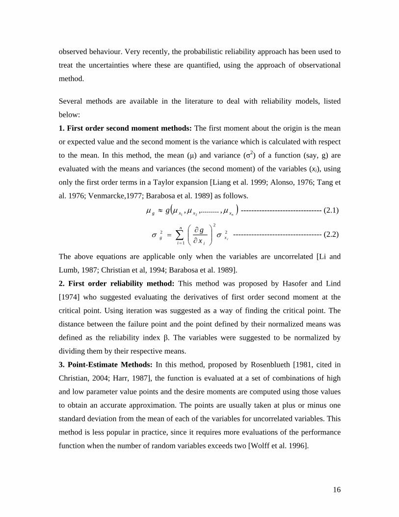
1. First order second moment methods: The first moment about the origin is the mean
or expected value and the second moment is the variance which is calculated with respect
to the mean. In this method, the mean (μ) and variance (σ2) of a function (say, g) are
evaluated with the means and variances (the second moment) of the variables (xi), using
only the first order terms in a Taylor expansion [Liang et al. 1999; Alonso, 1976; Tang et
al. 1976; Venmarcke,1977; Barabosa et al. 1989] as follows.
( )nxxxg g μμμμ ,,.........,
21≈ ------------------------------- (2.1)
22
1
2ix
n
i ig x
g σσ ∑=
⎟⎟⎠
⎞⎜⎜⎝
⎛∂∂
= ---------------------------------- (2.2)
The above equations are applicable only when the variables are uncorrelated [Li and
Lumb, 1987; Christian et al, 1994; Barabosa et al. 1989].
2. First order reliability method: This method was proposed by Hasofer and Lind
[1974] who suggested evaluating the derivatives of first order second moment at the
critical point. Using iteration was suggested as a way of finding the critical point. The
distance between the failure point and the point defined by their normalized means was
defined as the reliability index β. The variables were suggested to be normalized by
dividing them by their respective means.
3. Point-Estimate Methods: In this method, proposed by Rosenblueth [1981, cited in
Christian, 2004; Harr, 1987], the function is evaluated at a set of combinations of high
and low parameter value points and the desire moments are computed using those values
to obtain an accurate approximation. The points are usually taken at plus or minus one
standard deviation from the mean of each of the variables for uncorrelated variables. This
method is less popular in practice, since it requires more evaluations of the performance
function when the number of random variables exceeds two [Wolff et al. 1996].
16
4. Monte Carlo Simulation: In this method, a large number of discrete values are
generated from the underlying distribution to replace each continuous variable and used
to compute a large number of values of performance function and its distribution
[Chowdhury and Xu, 1995; Wong 1985; Cho, 2007]. A factor of safety corresponding to
each set is then calculated and plotted on a probability paper to determine their
distribution. The reliability index (β) and the probability of failure (Pf) are calculated
using the probability distribution of the factor of safety. The method can easily be
programmed for explicit performance function with simulation software such as the
Excel add-in @ RISK [EI-Ramly, 2002; Duncan, 2003], but for implicit functions (such
as slope stability analysis) an additional special program is required. The accuracy of this
method increases with the number of iterations, but not proportionally.
5. Other methods: Some other methods exist in the literature, such as second order
second moment or the second order reliability method, where higher order
approximations are considered [Christian, 2004].
2.7 Developed methods for pavement risk analysis
Some methods have been developed in the last few decades to incorporate reliability in
pavement design when there is uncertainty in the design data. Some research work in this
area is also available in the literature. The available methods and research studies are
reviewed and briefly described below.
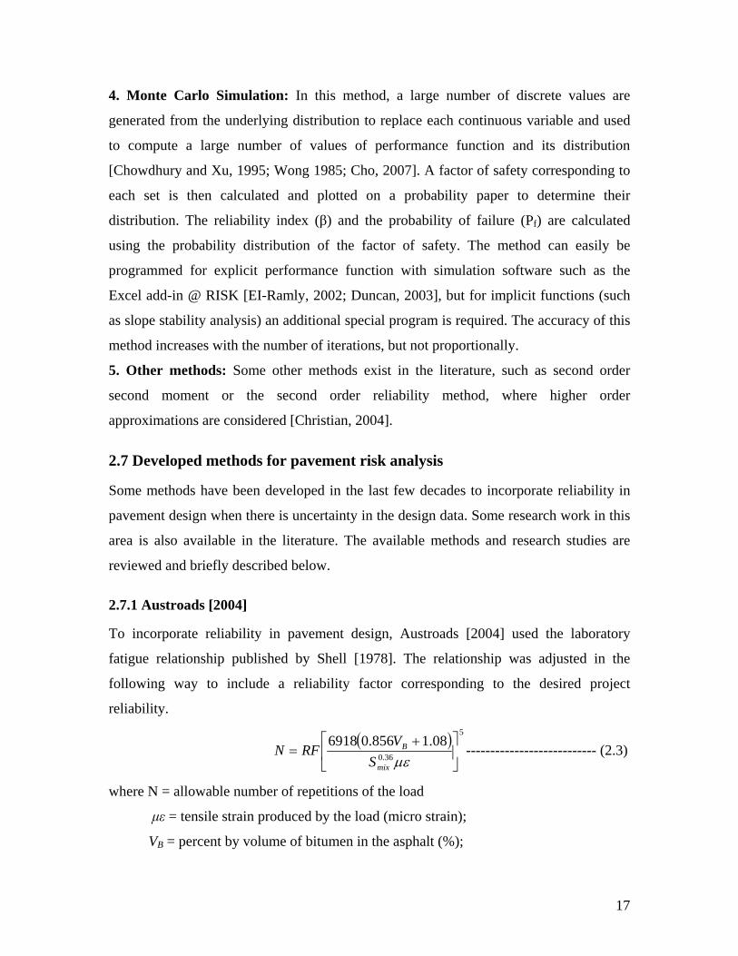
2.7.1 Austroads [2004]
To incorporate reliability in pavement design, Austroads [2004] used the laboratory
fatigue relationship published by Shell [1978]. The relationship was adjusted in the
following way to include a reliability factor corresponding to the desired project
reliability.
( ) 5
36.0
08.1856.06918⎥⎦
⎤⎢⎣
⎡ +=
μεmix
B
SVRFN --------------------------- (2.3)
where N = allowable number of repetitions of the load
με = tensile strain produced by the load (micro strain);
VB = percent by volume of bitumen in the asphalt (%);
17
Smix = asphalt modulus (MPa); and
RF = reliability factor for asphalt fatigue
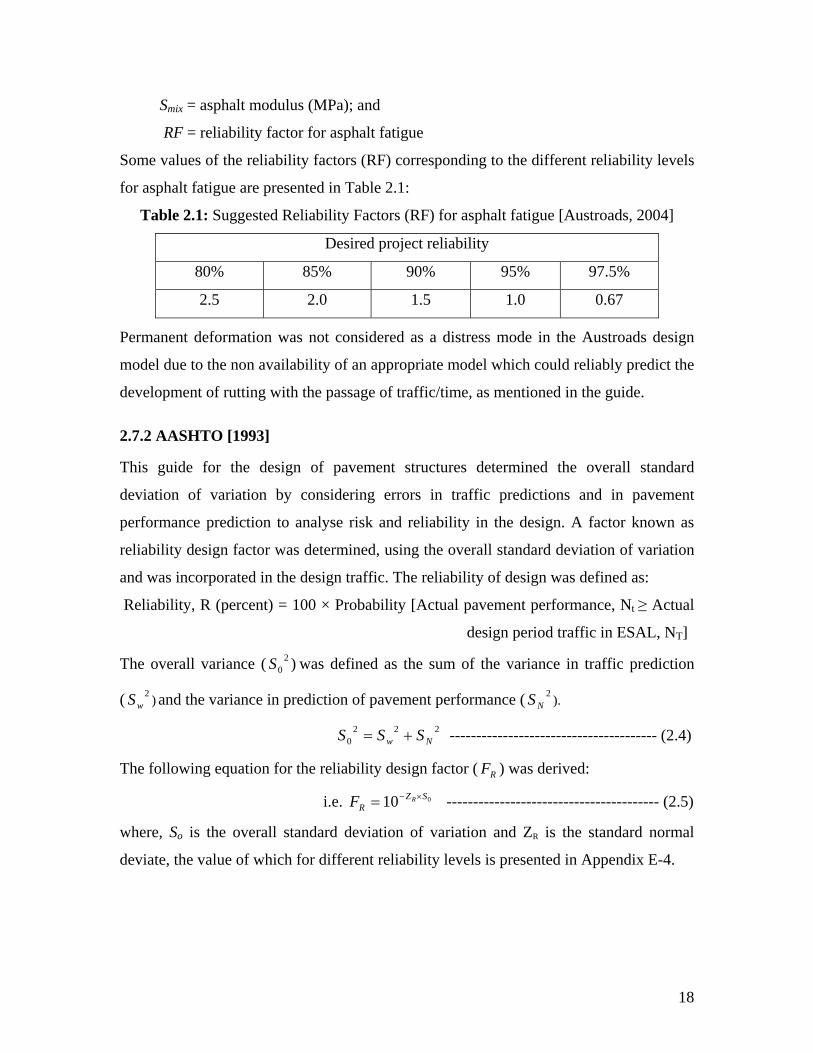
Some values of the reliability factors (RF) corresponding to the different reliability levels
for asphalt fatigue are presented in Table 2.1:
Table 2.1: Suggested Reliability Factors (RF) for asphalt fatigue [Austroads, 2004]
Desired project reliability
80% 85% 90% 95% 97.5%
2.5 2.0 1.5 1.0 0.67
Permanent deformation was not considered as a distress mode in the Austroads design
model due to the non availability of an appropriate model which could reliably predict the
development of rutting with the passage of traffic/time, as mentioned in the guide.
2.7.2 AASHTO [1993]
This guide for the design of pavement structures determined the overall standard
deviation of variation by considering errors in traffic predictions and in pavement
performance prediction to analyse risk and reliability in the design. A factor known as
reliability design factor was determined, using the overall standard deviation of variation
and was incorporated in the design traffic. The reliability of design was defined as:
Reliability, R (percent) = 100 × Probability [Actual pavement performance, Nt ≥ Actual
design period traffic in ESAL, NT]
The overall variance ( was defined as the sum of the variance in traffic prediction
( ) and the variance in prediction of pavement performance ( ).
)20S
2wS 2
NS
--------------------------------------- (2.4) 2220 Nw SSS +=
The following equation for the reliability design factor ( ) was derived: RF
i.e. ---------------------------------------- (2.5) 010 SZR
RF ×−=
where, So is the overall standard deviation of variation and ZR is the standard normal
deviate, the value of which for different reliability levels is presented in Appendix E-4.
18
To estimate the variance in traffic prediction ( ) and the variance in pavement
performance prediction ( ) the following approach was proposed by Noureldin et al.
[1994, 1996] and Huang [1993].
2wS
2NS
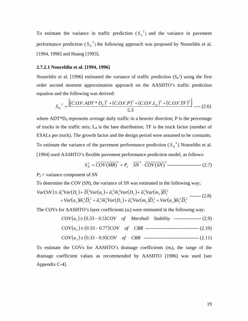
2.7.2.1 Noureldin et al. [1994, 1996]
Noureldin et al. [1996] estimated the variance of traffic prediction (SW2) using the first
order second moment approximation approach on the AASHTO’s traffic prediction
equation and the following was derived:
( ) ( ) ( ) ( )[ ]
3.5.........*... 2222
2 TFVOCLVOCPVOCDADTVOCS dd
W+++
= ---- (2.6)
where ADT*Dd represents average daily traffic in a heavier direction; P is the percentage
of trucks in the traffic mix; Ld is the lane distribution; TF is the truck factor (number of
ESALs per truck). The growth factor and the design period were assumed to be constants.
To estimate the variance of the pavement performance prediction ( ) Noureldin et al.
[1994] used AASHTO’s flexible pavement performance prediction model, as follows:
2NS
22
2
22 )()( SNCOVSNPMRCOVS N ⋅+= --------------------- (2.7)
P2 = variance component of SN
To determine the COV (SN), the variance of SN was estimated in the following way;
( ) ( ) ( ) ( ) ( )( ) ( ) ( ) ( ) 2
32
332
33233
23
23
22
222
222
222
22
221
211
21
DmaVarDmVaraDVarmaDmaVar
DmVaraDVarmaaVarDDVaraSNVar
++++
+++≅ ------- (2.8)
The COVs for AASHTO’s layer coefficients (ai) were estimated in the following way:
----------------- (2.9)
( ) ( ) StabilityMarshallofCOVaCOV 5.033.01 −≅
--------------------------------- (2.10)
the COVs for AASHTO’s drainage
( ) ( ) CBRofCOVaCOV 77.033.02 −≅
---------------------------------- (2.11) ( ) ( ) CBRofCOVaCOV 9.033.03 −≅
To estimate coefficients (mi), the range of the
drainage coefficient values as recommended by AASHTO [1986] was used [see
Appendix C-4].
19
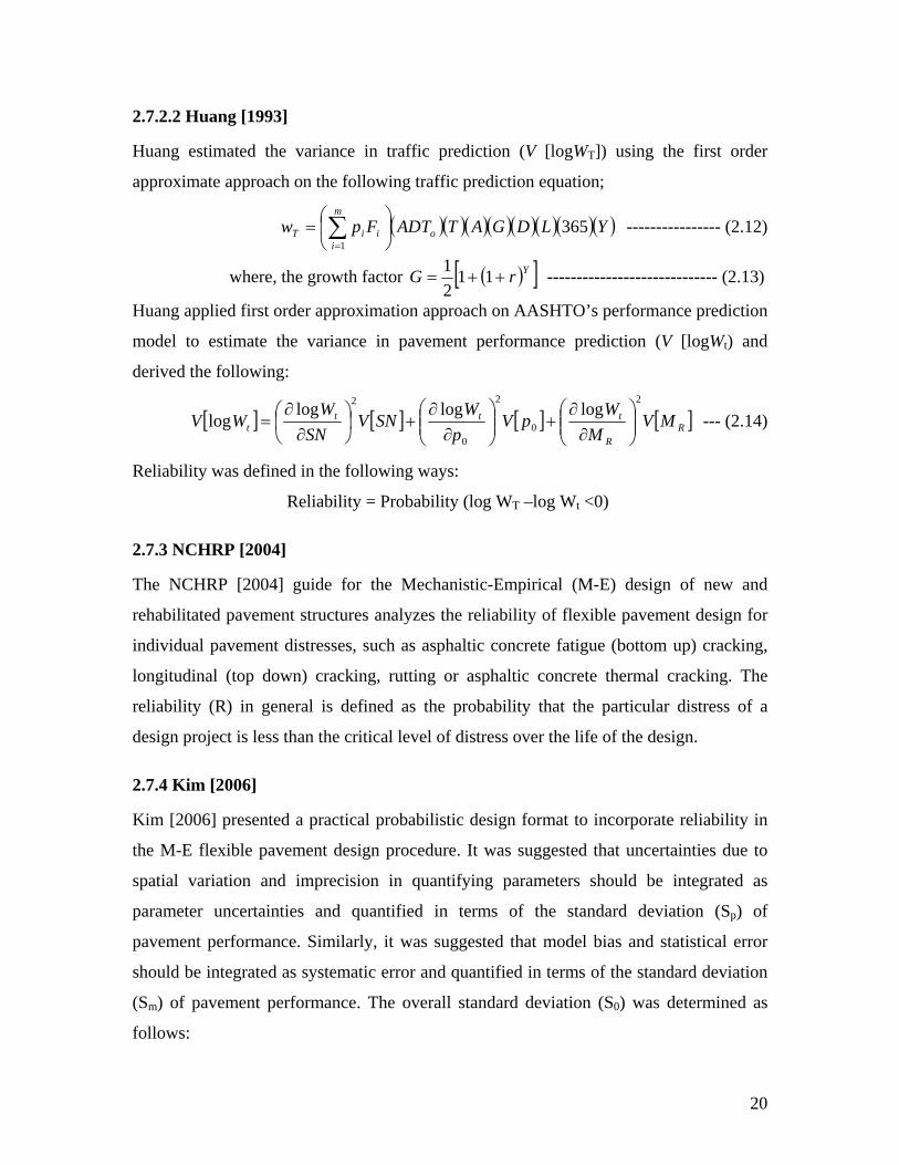
2.7.2.2 Huang [1993]
Huang estimated the variance in traffic prediction (V [logWT]) using the first order
approximate approach on the following traffic prediction equation;
---------------- (2.12) ( )( )( )( )( )( )( )( )YLDGATADTFpw o
m
iiiT 365
1⎟⎠
⎞⎜⎝
⎛= ∑
=
where, the growth factor ( )[ ]YrG ++= 1121 ----------------------------- (2.13)
Huang applied first order approximation approach on AASHTO’s performance prediction
model to estimate the variance in pavement performance prediction (V [logWt) and
derived the following:
[ ] [ ] [ ] [ RR
tttt MV
MW
pVp
WSNV
SNW
WV2
0
2
0
2 loglogloglog ⎟⎟
⎠
⎞⎜⎜⎝
⎛∂
∂+⎟⎟
⎠
⎞⎜⎜⎝
⎛∂
∂+⎟
⎠⎞
⎜⎝⎛
∂∂
= ] --- (2.14)
Reliability was defined in the following ways:
Reliability = Probability (log WT –log Wt <0)
2.7.3 NCHRP [2004]
The NCHRP [2004] guide for the Mechanistic-Empirical (M-E) design of new and
rehabilitated pavement structures analyzes the reliability of flexible pavement design for
individual pavement distresses, such as asphaltic concrete fatigue (bottom up) cracking,
longitudinal (top down) cracking, rutting or asphaltic concrete thermal cracking. The
reliability (R) in general is defined as the probability that the particular distress of a
design project is less than the critical level of distress over the life of the design.
2.7.4 Kim [2006]
Kim [2006] presented a practical probabilistic design format to incorporate reliability in
the M-E flexible pavement design procedure. It was suggested that uncertainties due to
spatial variation and imprecision in quantifying parameters should be integrated as
parameter uncertainties and quantified in terms of the standard deviation (Sp) of
pavement performance. Similarly, it was suggested that model bias and statistical error
should be integrated as systematic error and quantified in terms of the standard deviation
(Sm) of pavement performance. The overall standard deviation (S0) was determined as
follows:
20
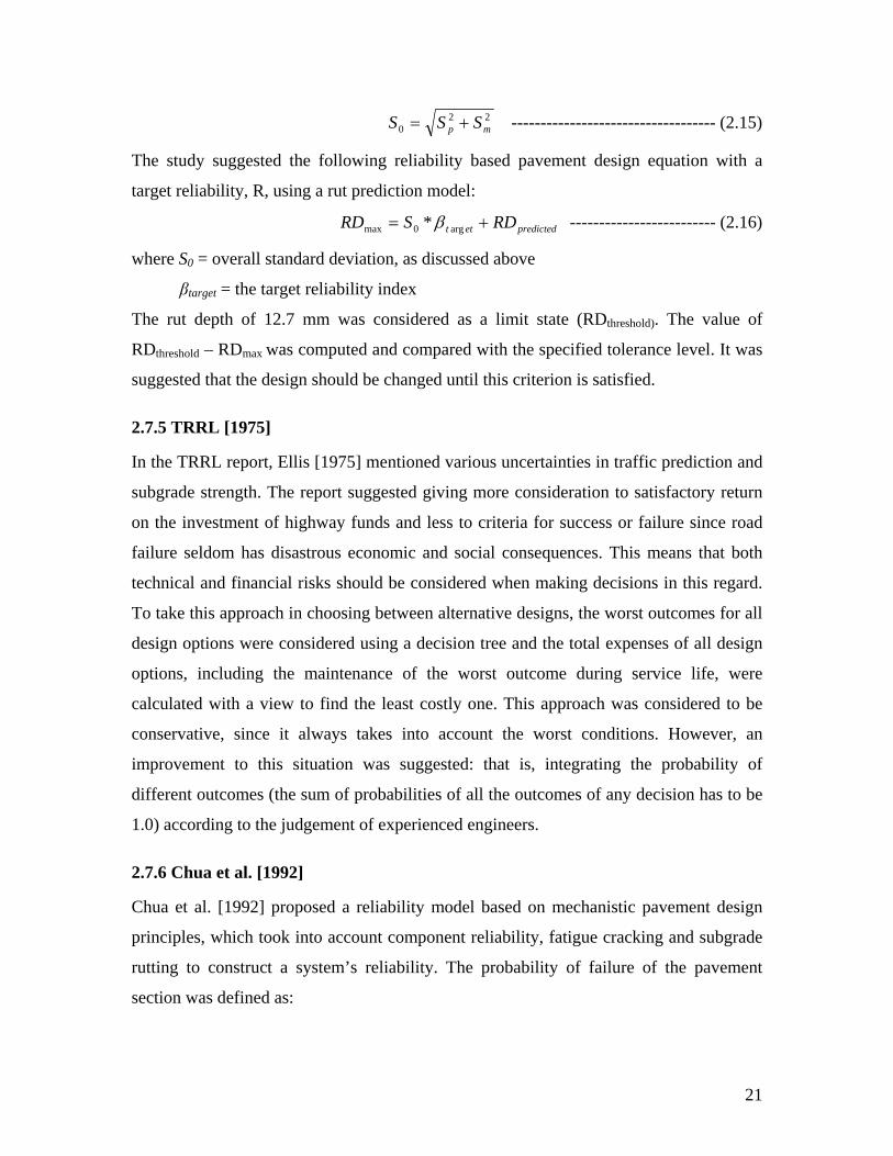
220 mp SSS += ----------------------------------- (2.15)
The study suggested the following reliability based pavement design equation with a
target reliability, R, using a rut prediction model:
ettSRD predictedRD+= arg0max *β ------------------------- (2.16)
where S viation, as discussed above
ed as a limit state (RDthreshold). The value of
2.7.5 TRRL [1975]
Ellis [1975] mentioned various uncertainties in traffic prediction and
2.7.6 Chua et al. [1992]
sed a reliability model based on mechanistic pavement design
0 = overall standard de
βtarget = the target reliability index
The rut depth of 12.7 mm was consider
RDthreshold – RDmax was computed and compared with the specified tolerance level. It was
suggested that the design should be changed until this criterion is satisfied.
In the TRRL report,
subgrade strength. The report suggested giving more consideration to satisfactory return
on the investment of highway funds and less to criteria for success or failure since road
failure seldom has disastrous economic and social consequences. This means that both
technical and financial risks should be considered when making decisions in this regard.
To take this approach in choosing between alternative designs, the worst outcomes for all
design options were considered using a decision tree and the total expenses of all design
options, including the maintenance of the worst outcome during service life, were
calculated with a view to find the least costly one. This approach was considered to be
conservative, since it always takes into account the worst conditions. However, an
improvement to this situation was suggested: that is, integrating the probability of
different outcomes (the sum of probabilities of all the outcomes of any decision has to be
1.0) according to the judgement of experienced engineers.
Chua et al. [1992] propo
principles, which took into account component reliability, fatigue cracking and subgrade
rutting to construct a system’s reliability. The probability of failure of the pavement
section was defined as:
21
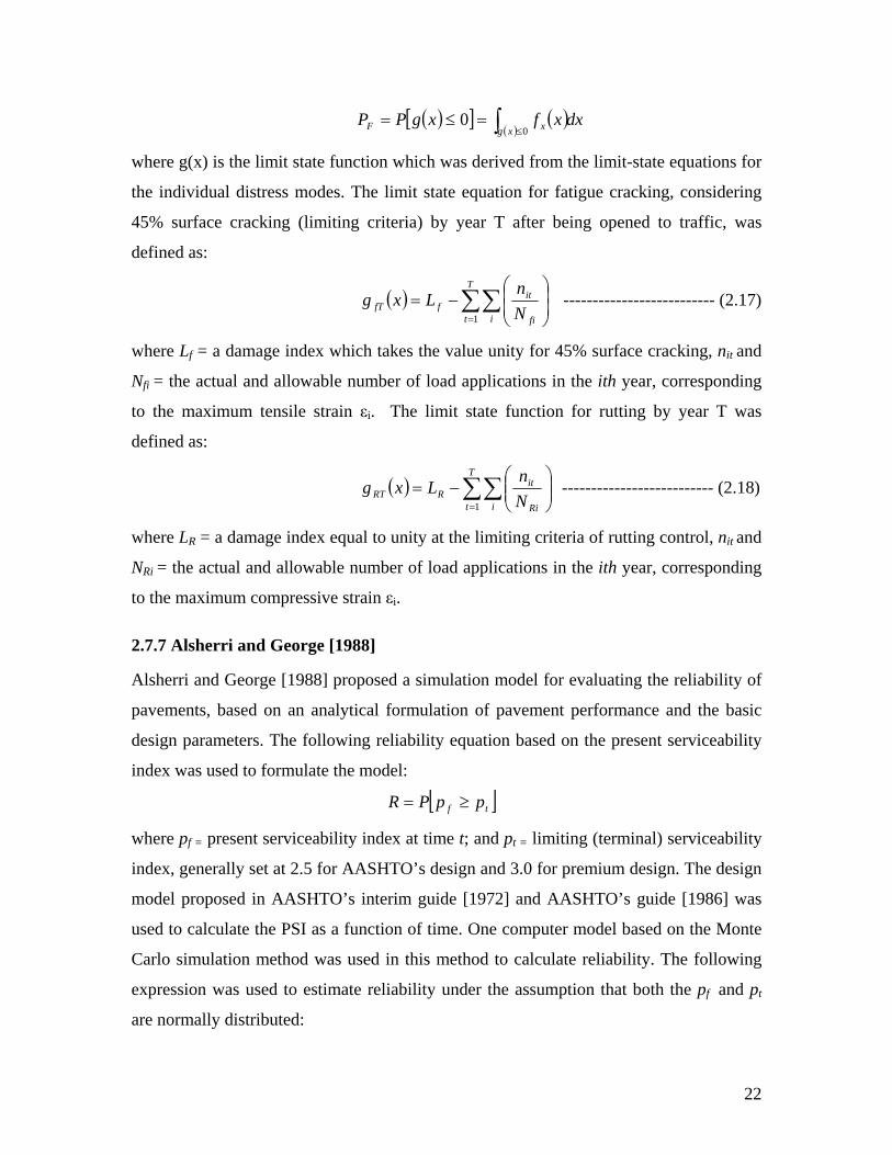
( )[ ] ( )( )
dxxfxgPPxg xF ∫ ≤
=≤=0
0
where g(x) is the limit state function which was derived from the limit-state equations for
the individual distress modes. The limit state equation for fatigue cracking, considering
45% surface cracking (limiting criteria) by year T after being opened to traffic, was
defined as:
( ) ∑∑=
⎟⎟⎠
⎞⎜⎜⎝
⎛−=
T
t i fi
itffT N
nLxg
1 -------------------------- (2.17)
where Lf = a damage index which takes the value unity for 45% surface cracking, nit and
Nfi = the actual and allowable number of load applications in the ith year, corresponding
to the maximum tensile strain εi. The limit state function for rutting by year T was
defined as:
( ) ∑∑=
⎟⎟⎠
⎞⎜⎜⎝
⎛−=
T
t i Ri
itRRT N
nLxg
1
-------------------------- (2.18)
where LR = a damage index equal to unity at the limiting criteria of rutting control, nit and
2.7.7 Alsherri and George [1988]
d a simulation model for evaluating the reliability of
NRi = the actual and allowable number of load applications in the ith year, corresponding
to the maximum compressive strain εi.
Alsherri and George [1988] propose
pavements, based on an analytical formulation of pavement performance and the basic
design parameters. The following reliability equation based on the present serviceability
index was used to formulate the model:
[ ]tf ppP ≥R =
x at time t; and limiting (terminal) serviceability
are normally distributed:
where pf = present serviceability inde pt =
index, generally set at 2.5 for AASHTO’s design and 3.0 for premium design. The design
model proposed in AASHTO’s interim guide [1972] and AASHTO’s guide [1986] was
used to calculate the PSI as a function of time. One computer model based on the Monte
Carlo simulation method was used in this method to calculate reliability. The following
expression was used to estimate reliability under the assumption that both the pf and pt
22
( ) ( )02/122zR
ptpf
ptpf φσσ
μμ ⎤⎡ −φ =
⎥⎥
⎦⎢⎢
⎣ +=
distribution; μpf, μpt = mean value of pf and pt; σpf, σpt =
standard deviations of pf and pt; and z0 = standard normal deviate.
where Ф = standard normal
The following formulation was suggested to calculate the reliability defined above.
dzzz⎟⎞
⎜⎛ −01 2
R ∫ ∞− ⎟⎠
⎜⎝Π
=2
exp2
--------------------------- (2.19 )
Kulkarni [1994] presented a methodology which chose traffic as a design element for
in evaluating the reliability of alternate pavement designs with
-
eviation (SD) of
2.7.8 Kulkarni [1994]
incorporating reliability
different types of pavements. The reliability R of a pavement design was defined as:
R = probability [actual traffic load capacity, N > actual cumulative traffic, n], or
R = probability [ln N > ln n] = probability [ln N – ln n > 0]
ln N and ln n, it was suggested, would follow normal distribution since N and n are log
normally distributed. The safety margin (SM) of design was defined as:
SM = ln N- ln n ----------------------------------- (2.20)
The reliability index (β), defined as the ratio of mean (E) and standard d
safety margin (SM), was then used as a suitable measure for design reliability.
[ ][ ]SMSDSME
=β [ ] [ ][ ] [ ]nN
nENElnvarlnvar
lnln+−
= ----------------------- (2.21)
2.7.9 Zhang [2006]
Zhang [2006] investigated the applicability of the method of moments as a technique for
ability of failure in order to develop a reliability function for
(X, t) = time dependent limit state function for n basic random variables X =
tress as accumulated
estimating the prob
pavement infrastructure. A limit state function, where the functional forms of strength
and stress were defined separately, was considered in the investigation, which was as
follows:
G (X, t) = strength – stress (t)
where G
[x1... xn]T. Strength was defined as allowable use before failure and s
23
use at time t. The failure event was defined as {G(X, t) ≤ 0} and the probability of failure
pF (t) was expressed as a time-dependent multidimensional failure state integral for the
failure event as follows:
( ) ( )[ ] ( )dXtXftXGobtpF ∫=≤= ,0,Pr XG ≤0)(
where f (X, t) was defined as a time dependent joint probability density function of the
X. The method of moments (first four moments) was used to
Lua et al. [1996] investigated the effects of spatial variability on finite-element pavement
the predicted service life, for airfield pavements in particular.
Brown [1994] reviewed the advantages and disadvantages of the reliability methodology.
gy was defined as the process of estimating and correctly
basic random variables
evaluate the above integral.
2.7.10 Lua et al. [1996]
response analysis and on
Theories of statistics and structural reliability were combined in the investigation and it
was termed probabilistic finite element analysis. Random spatial variability in the layered
material properties was characterized by multiple random fields and random variables
were used to characterize the uncertainties in external loads and in pavement geometry.
2.7.11 Brown [1994]
Reliability methodolo
combining all the uncertainties associated with a particular design model into an overall
variance. It was suggested that the overall uncertainty in the mathematical system could
be determined if the uncertainty in each portion could be estimated. In this procedure, the
sensitivity of the output to each input variable (considering other uncertainties also) was
compared by means of a sensitivity analysis. It was also suggested that a safety factor
should be applied as convenient. The process required only information on the number of
deviations away from the mean that the design should consider. For this purpose,
consulting the opinions of expert designers was suggested. The mean plus two standard
deviations was suggested as the best design option for rural secondary roads and mean
plus four standard deviations for urban freeways [Brown et al., 1970; cited in Brown,
1994].
24
2.8 Developed methods for embankment risk analysis
Geotechnical engineers are now recognizing the fact that some significant uncertainties
able investigation effort or
expenditure [Chowdhury and Xu, 1995]. Hence, some methods of risk analysis have been
l engineering was conventionally a matter of applying
enting local experience and
engineering judgment. But the safety factor is not a consistent measure of risk. Historical
ires more data, time and
ature demonstrating the merits and use of
mance is not well defined and there is
the probabilistic theory started to be used in the 1970s
atic
inherent in embankment design cannot be removed by reason
developed in the last few decades with regard to embankment slope stability and
settlement. The present study reviewed the existing risk analysis methods and presents a
brief summary of them below.
2.8.1 Developed methods of slope stability risk analysis
The uncertainty in geotechnica
factors of safety (deterministic analysis) or of implem
analysis shows that such apparently conservative design is not proof against failure. In
particular when proper consideration is not given to uncertainty, considering the safety
factor alone gives a misleading sense of safety [Li and Lumb, 1987]. Probabilistic
concepts and methods are excellent tools to quantify uncertainty and incorporate it in the
design process. Although the benefits of probabilities analysis were identified long ago,
few designers have implemented it. EI-Ramly [2002] identified the following reasons for
designers to choose deterministic analysis over probabilistic:
1) Designers do not usually feel confident in dealing with probabilities, due to their
lack of sufficient statistical knowledge.
2) It is wrongly assumed that probabilistic analysis requ
effort than deterministic.
3) Lack of sufficient documents in the liter
probabilistic analysis.
4) The tolerable range of unsatisfactory perfor
no link between deterministic and probabilistic assessment.
In geotechnical engineering,
[Juang et al., 1998]. Since then, numerous studies of probabilistic slope stability analysis
have been undertaken to deal with the uncertainties of soil properties in a system
manner. They include work by Alonso [1976], Li and Lumb [1987], Tang et al. [1976],
25
Barabosa et al. [1989], Chowdhury and Xu [1995], Wong [1985], Juang et al. [1998] and
Xu and Low [2006] etc. In probabilistic slope stability analysis, the factor of safety,
defined as the ratio of resistance to driving forces on a potential sliding surface, is
determined deterministically and probabilistic reliability analysis is used to assess the
uncertainties in the factor of safety [Bhattacharya et al., 2003]. The factor of safety is
expressed in terms of its mean and variance [Malkawi et al., 2000]. The degree of
uncertainty in the calculated factor of safety is usually expressed with the reliability index
(β). A number of approaches is available in the literature for performing probabilistic risk
analysis, as discussed in section 2.6. The existing methods of probabilistic slope stability
risk analysis as found in the literature are briefly described below.
2.8.1.1 First-order second moment method
The first-order second moment method is mostly used for probabilistic slope stability
g et al. [1976], Venmarcke [1977], Li and
analysis. It includes Wu and Kraft [1970], Tan
Lumb [1987], Barabosa et al. [1989], Christian et al. [1994], Liang et al. [1999] and
many others. In the first order second moment reliability method, the expected value of
the performance function is calculated by evaluating the performance function using the
expected values of the parameters. The variance of the performance function is computed
by summing the products of the partial derivatives of the performance function at the
mean parameter values and the variance of the corresponding parameters. In slope
stability risk analysis with this method, the slope geometry and the probability
distribution of soil properties (Ф, c and γ) are specified first. Then the critical slip surface
and its associated factor of safety are determined, using limit equilibrium methods
[Bishop, 1955; Janbu, 1968 and Spencer, 1967]. The partial derivatives of the factor of
safety with respect to each of the soil properties are then evaluated. Next, the mean and
variance of the factor of safety are calculated. Finally, the reliability index (β) and the
probability of failure (Pf) of the slope are calculated. The Reliability index is defined as
[ ][ ]F
FEσ
β 0.1−= OR [ ]
[ ] [ ]FCovFEFE.
0.1−=β ---------------------- (2.22)
where β is reliability in puted factor of safety. The Reliability index dex and F is com
normalizes the factor of safety with respect to its standard deviation. It defines the
26
number of standard deviations F (safety) is away from its failure value of 1.0. A higher
value of β means lower probability of failure.
2.8.1.2 Point estimation method
The point estimation method developed by Rosenblueth [in Harr, 1987] could be used as
n [Liang et al., 1999; Li and Lumb 1987; Barabosa et
Chowdhury and Xu [1995], Cho [2007] and some others have recently used the Monte
lope stability analysis. In the Monte Carlo simulation
probabilistic slope stability risk analysis also available in
t order second moment method is used in a different way; or
an alternative to Taylor’s expansio
al., 1989] where the moments of the performance function are determined by evaluating
it as a set of combinations of high and low parameter values and weighting the results by
factors. Although this method better captures the behaviour of the nonlinear functions, it
is not popular in practice since many evaluations of the performance are required for
more than two random variables. In addition, both Taylor’s series and the point estimate
method are not invariance for nonlinear performance functions and yield different values
for the reliability index when the performance function and limit state can be expressed in
different equivalent ways (say, force/resistance=1 or force-resistance=0). Hasofer and
Lind [1974] developed an invariant reliability index determination procedure, where
Taylor’s series was expanded about an unknown point termed the failure point and an
iterative process was used to solve it. However, many researchers were unwilling to use
it, probably due to its complexity [Tang et al., 1976; Christian, 1994; Venmarcke, 1977].
2.8.1.3 Monte Carlo simulation
Carlo simulation in probabilistic s
method, the slope geometry and the probability distribution of soil properties (Ф, c and γ)
are specified first. Then independent sets of soil properties (Ф, c and γ) are generated
from their assigned probability distributions. The Limit equilibrium method [Bishop,
1955; Janbu, 1968; or Spencer, 1967] is used to calculate the factor of safety for each set,
after which the mean, the standard deviation and associated probability distribution of the
factor of safety are determined. Accordingly, the Reliability index (β) and the probability
of failure (Pf) are evaluated.
Some other research work on
the literature; in this the firs
27
the Monte Carlo simulation method is used with the finite element method; or fuzzy sets
are used to address the uncertainties. Such as Christian et al. [1994], Liang et al. [1999],
Griffiths and Fenton [2004], Juang et al. [1998], and Xu and Low [2006]. A brief
summary of these methods is presented below.
2.8.1.4 Mean first order reliability method
Christian et al. [1994] simplified the general first order reliability method by proposing
ethod, the derivatives of the first order
iability is averaged over the failure surface in case of a
mited number of tests. Larger numbers of
rce of uncertainty or error could result from the
, for example, the use of two-
Liang et al. [1999] proposed a reliability-based algorithm for calculating the risk in slope
proach was
the mean first order reliability method. In this m
second moment method are evaluated at the mean value of variables. To apply this
method, Christian et al. [1994] divided the uncertainties which affect the stability of slope
into the two following categories:
1) Data scatter: uncertainties due to real spatial variation and random testing error were
termed data scatter. The spatial var
long failure surface and creates less uncertainty. Hence a reduction factor f was suggested
by many researchers [EI-Ramly et al., 2002].
2) Systematic error: two types of systematic error were identified:
a) Statistical error in the mean due to a li
tests yield different results.
b) Bias due to the experimental procedure itself.
It was suggested that another sou
simplification and assumptions made in the design
dimensional analyses instead of three-dimensional, failure to find the most critical failure
surface and error associated with numerical and rounding. An investigation carried out by
Azzouz et al. [1983] showed that all these factors increased the mean factor of safety by
5% and impart a variation which could be estimated as COV of 0.07.
2.8.1.5 Risk analysis algorithm with Fellenius limit equilibrium method
design where the first order second moment (FOSM) probabilistic ap
implemented into the Fellenius limit equilibrium method so as to derive the performance
function and reliability index. The probability of failure was defined as:
28
( ){ }0<= XgPPf
The performance function g(X) was formulated using the modified Fellenius method in
the following way;
( ) 0.1−= FXg
Then the reliability index, β was defined taking into account the performance function
and all the random variables normally distributed as:
g
g
σμ
β =
where μg and σg are the mean and standa atird devi on of the performance function, g(X).
The corresponding probability of failure was then described by:
( )βφ −=fP
where Ф (.) was the standard normal cumulative probability. The following equation of β
roposed: based on log normal distribution was p
( )( )2
2
1ln
1/ln
F
FF
V
V
+
+=
μβ ---------------------------------- (2.23)
respectively.
inistic approach using fuzzy set
Juang et al. [1998] proposed an easy deterministic approach to incorporate uncertainty in
: that of expressing the uncertainty
where μF and VF are the mean and co-efficient of variation of the factor of safety
2.8.1.6 Determ
soil parameters in the slope stability analysis
parameters as a fuzzy set. The fuzzy set was defined as pair values [x, μ(x)] where a
member x belongs to the set in a degree of μ(x), ranging from 0 to 1. A sub set of a fuzzy
set called a fuzzy number was used for routine geotechnical uncertainty modelling. Since,
in routine geotechnical practice, a statistical significant database is rarely available or too
costly to obtain, a fuzzy number, it was suggested, could be used to reflect the
uncertainty. The uncertainty could be incorporated in a fuzzy number by means of
engineering judgment based on available information.
29
2.8.1.7 Random finite element method
Griffiths and Fenton [2004] combined a nonlinear finite element analysis with random
field generation techniques for the reliability analysis of simple homogeneous slopes and
termed the method the random finite element method. The method fully accounts for
spatial correlation and averaging and a powerful slope stability analysis tool which does
not require previous assumptions about the shape or location of the failure surface. The
Monte Carlo simulation was used to calculate the failure probability.
Wong [1985] also used the Monte Carlo simulation together with a finite-element method
to calculate the probability of failure of a homogeneous slope. However, the computation
of the failure probability was reported as costly when there are many input variables.
2.8.1.8 Finite-element method with the first-order reliability method
Xu and Low [2006] proposed a procedure for probabilistic slope stability analysis for
embankments by integrating a finite-element method and first-order reliability method
(FORM), which is not restricted to any specific stability analysis method.
2.8.2 Developed methods of settlement risk analysis
Very few methods have been developed for the risk analysis of embankment settlement.
A brief summary of a developed method as found in the literature for the risk analysis of
soil settlement is presented below.
2.8.2.1 Fenton and Griffiths [2002]
Fenton and Griffiths [2002] proposed a probabilistic approach to a settlement risk
analysis where the reliability of the foundation was assessed against the probability of
excessive settlement for a single spread footing and the probabilities of excessive
differential settlement for a paired spread footing. The elastic modulus of soil was
considered as the main variable in soil properties. In this approach, the deterministic
settlement (δdet) was determined first, by using a finite element analysis including an
invariant soil modulus. Then the variance of log-elastic soil modulus ( ) was
determined. Next, using these values and the variance function of width (Wf) and depth
2ln Eσ
30
(H) of foundation [γ(Wf, H)], the mean ( δμ ln ) and the variance of log-settlement ( δσ ln )
were determined as follows:
( ) 2lndetln 2
1 --------------------------- (2.24) ln δ= Eσμ δ +
( ) 2lnln , Ef HWand σγσ δ = -------------------------- (2.25)
They used a computer program to estimate the covariance between local averages of log-
Risk of settlement failure = P [|Δ| > limiting value] -------------- (2.
2.9 Quality control and quality assurance
ess which is undertaken to ensure that a
conditions in Bangladesh.
elastic modulus (Clnδ). Then the mean, standard deviation and correlation coefficient of
actual settlement under each footing was calculated and, using these values, the mean and
variance of differential settlement (Δ) were calculated. Finally, the mean absolute
settlement (|Δ|) was predicted and the risk of structure failure for settlement was
described as the probability of mean absolute settlement greater than the limiting value.
That is,
26)
Quality Control in highway construction is a proc
highway pavement or embankment is constructed according to the specifications given in
the design. In quality control, the degree of compliance with the standard specifications
of the completed works is also assessed, providing a means by which the work can be
accepted or rejected in accordance with the prescribed standards. Not all materials and
construction are exactly the same and they are always subject to some variation, which
may or may not be acceptable. Therefore, this variability should be taken into account in
formulating the methodology of quality control procedure so that a high level of
confidence can be assumed so long as sampling and testing have been carried out
properly. Consequently, the highway quality assurance methods based on mathematical
models and statistical concepts have progressed from the early materials-and-methods
specifications through statistical end-result specifications to the current trend towards
performance-related specifications (PRS) [Weed, 2006]. A number of such methods for
highway pavement are described in more detail in Chapter 8 and for highway
embankment in Chapter 9 with a view to developing methodology suitable for the
31
In many cases, the data from quality-control tests are not used to correct deficiencies if
they are present during construction. As mentioned previously, quality control enables
ses where the specified level of quality has not been achieved
ed by a large number of individual values,
the specification compliance of the pavement being constructed to be determined. This
quality check should be made continuously during the construction stage. It enables
modifications to be made to the original design to ensure that the pavement will perform
its intended function without reaching the terminal serviceability level before the end of
the design period.
Statistical end-result specifications usually suggest some sort of pay adjustments as
recompense in ca
[Pathomvanich, 2000; Douglas et al., 1999; Dobrowolski and Bressette, 1998]. In such
cases a contractor’s pay may be adjusted according to the level of quality actually
achieved in relation to what was specified. The objective of such schemes is to cover the
extra cost expected to remedy work which is initially deficient in quality by withholding
sufficient payment at the time of construction. For example, if the construction work is
below an acceptable standard a pavement may not be capable of carrying the design
loading and thus has more chance of failing before the end of the design period. The
resulting unplanned maintenance activities result in an additional expense to the highway
agency and society as a whole because such repairs generally occur some time after the
contractual obligations, if any, have expired.
Since no materials and construction processes are entirely homogeneous, any particular
property of a material or work can be describ
which will vary according to some type of distribution. Usually, these individual values
can be represented by a population with a normal distribution, having a mean value and a
standard deviation, with sufficient practical accuracy. The acceptance decision is based
on a small number of tests made on samples or made at selected locations, since no
highway agency can test the entire material or construction. The true mean of the results
of all possible tests that could be made on an entire material or construction will seldom,
or never, coincide with the computed average of test results from the small number of test
samples. Further, there is a possibility that the test may belong to a population which is
either acceptable or unacceptable in terms of specification. The probability of rejecting
acceptable work based on a small number of tests is known as Type I error and
32
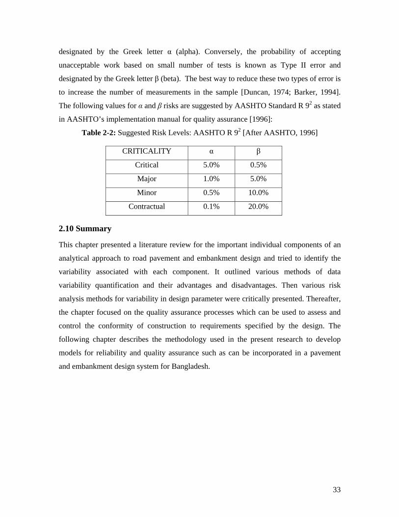
designated by the Greek letter α (alpha). Conversely, the probability of accepting
unacceptable work based on small number of tests is known as Type II error and
designated by the Greek letter β (beta). The best way to reduce these two types of error is
to increase the number of measurements in the sample [Duncan, 1974; Barker, 1994].
The following values for α and β risks are suggested by AASHTO Standard R 92 as stated
in AASHTO’s implementation manual for quality assurance [1996]:
Table 2-2: Suggested Risk Levels: AASHTO R 92 [After AASHTO, 1996]
CRITICALITY α β
Critical 5.0% 0.5%
Major 1 5.0% .0%
Minor 0.5% 10.0%
Co al ntractu 0.1% 20.0%
2.10 Summary
This chapter presented a literature review for the important individual components of an
h to road pavement and embankment design and tried to identify the
analytical approac
variability associated with each component. It outlined various methods of data
variability quantification and their advantages and disadvantages. Then various risk
analysis methods for variability in design parameter were critically presented. Thereafter,
the chapter focused on the quality assurance processes which can be used to assess and
control the conformity of construction to requirements specified by the design. The
following chapter describes the methodology used in the present research to develop
models for reliability and quality assurance such as can be incorporated in a pavement
and embankment design system for Bangladesh.
33
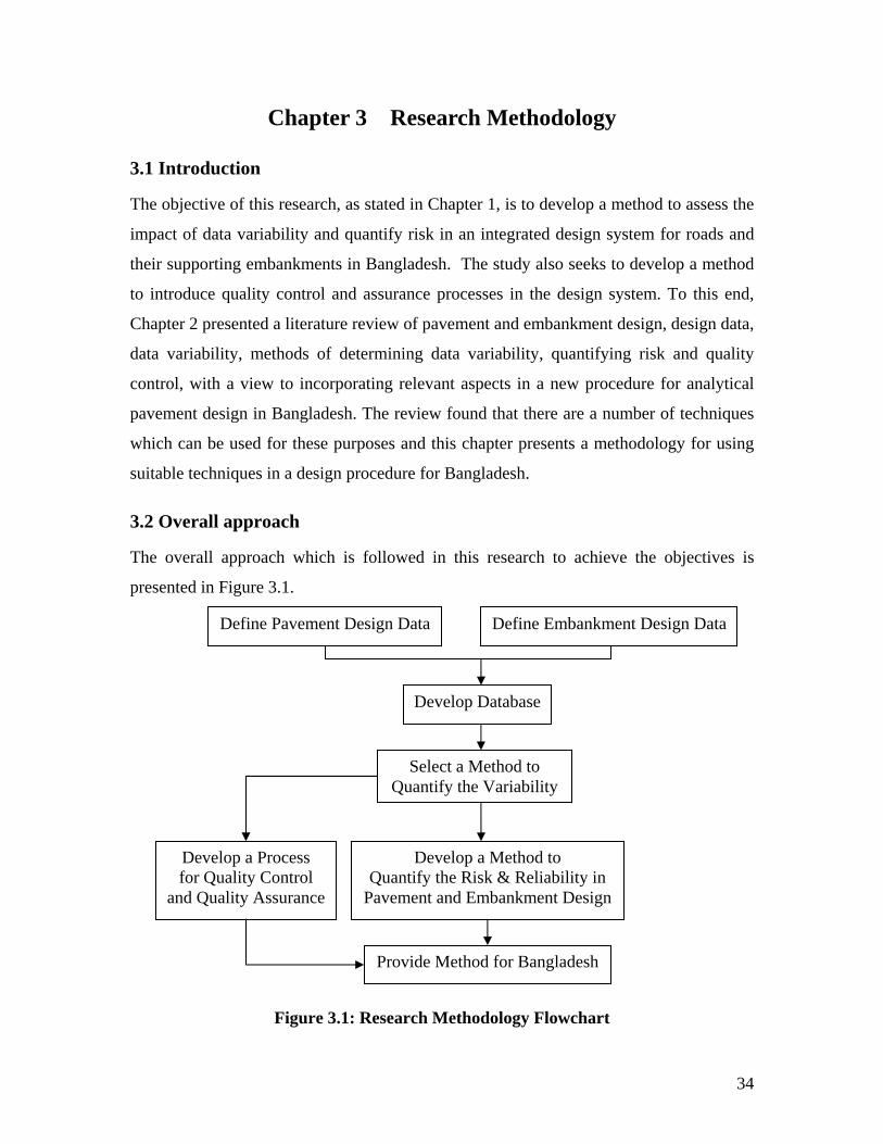
Chapter 3 Research Methodology
3.1 Introduction
The objective of this research, as stated in Chapter 1, is to develop a method to assess the
bility and quantify risk in an integrated design system for roads and
The overall approach which is followed in this research to achieve the objectives is
Figure 3.1: Research Methodology Flowchart
impact of data varia
their supporting embankments in Bangladesh. The study also seeks to develop a method
to introduce quality control and assurance processes in the design system. To this end,
Chapter 2 presented a literature review of pavement and embankment design, design data,
data variability, methods of determining data variability, quantifying risk and quality
control, with a view to incorporating relevant aspects in a new procedure for analytical
pavement design in Bangladesh. The review found that there are a number of techniques
which can be used for these purposes and this chapter presents a methodology for using
suitable techniques in a design procedure for Bangladesh.
3.2 Overall approach
presented in Figure 3.1.
Define Pavement Design Data Define Embankment Design Data
Develop Database
Select a Method to Quantify the Variability
Develop a Process for Quality Control
and Quality Assurance
Develop a Method to Quantify the Risk & Reliability in
Pavement and Embankment Design
Provide Method for Bangladesh
34
In this proc ment design data are identified first and a
database is developed with field evaluation. Then a method is selected to quantify the
variability in the design data. To quantify the risk in pavement and embankment design
due to variability in the design dat ethods and techniques are
investigated and a suitable method is identified and developed for Bangladesh. Similarly,
a suitable quality control process avement and embankment
construction in Bangladesh by invest ds and techniques. Finally,
the selected or developed methods are recommended for Bangladesh by presenting them
before ladeshi road their acceptability. The
detai oces
3.3 Database development
The quantification of design risk control process are
based on the variability of the design data. Hence, a database was required and was
on result from variations in: the average daily traffic in
heavier direction; the percentage of trucks in the traffic mix; the percentage of trucks in
in heavier direction
The traffic volume and load travelling on a road in either direction varies with the time of
day and season and this can have an impact on the load for which the design is calculated.
ess the pavement and embank
a, the available m
is developed for p
igating the existing metho
representative Bang engineers, to ensure
led description of this pr s is presented below.
and the requirements of a quality
subsequently developed in this research.
3.4 Pavement design data variability analysis
As described in Section 2.4 the major uncertainties associated with an analytical design
process for road pavements concern traffic, material characterisation and pavement
performance prediction. Uncertainty in pavement performance prediction results from
variability in climate, material properties, pavement layer thickness, pavement surface
condition evaluation and sub-grade stiffness. Detailed descriptions of these factors and
techniques which may be used to quantify them are summarised below.
3.4.1 Traffic prediction variation analysis
Uncertainties in traffic predicti
the design lane; and the number of ESALs per truck [Huang, 1993].
3.4.1.1 Variation in average daily traffic
35
Traffic growth rates also vary from year to year. For an accurate characterization of the
Sadeghi and Fathali, 2007]. The AASHTO road tests conducted in the 1950s [AASHTO,
proportional to the axle load raised to the
ing countries, where an
raffic composition may be distributed differently across
has suggested
use in Bangladesh. These may be used to determine the
traffic potential, the variations should be quantified. However, this may be problematic in
Bangladesh where traffic data for both directions are not usually available and it is usual
to assume that equally heavy traffic travels in both directions.
3.4.1.2 Axle load composition
Heavy loaded axles are the main contributor to pavement damage [AASHTO, 1993;
1986] suggested that pavement damage is
fourth power. Consequently, it is very important to be able to determine and quantify any
potential variation in the composition of the traffic in terms of axle loads.
The problem of over-loaded vehicles causing road pavements to deteriorate faster than
they were designed to is particularly apparent in many develop
increasing number of heavy and over-loaded axles move on national and regional
highways. Investigation by Maheri and Akbari [1993] indicates that this problem causes a
great deal of damage to road networks and results in noticeable unplanned maintenance
and repair costs [cited in Sadeghi and Fathali, 2007]. Therefore, the variation in axle load
should be quantified in the design risk analysis process.
3.4.1.3 Variation in percent of trucks in design lane
As mentioned previously, the t
the lanes on a multi-lane road, such as a motorway. Usually, the nearside lane is most
heavily loaded over the life of a pavement as it tends to carry most of the heavily laden
trucks. Where it is not possible to measure the distribution of traffic across a multi-lane
road, a variety of methods has been suggested for estimating the traffic using each lane
from the traffic data from one or more lanes. For example, Khan [2005]
lane distribution factors for
traffic in each lane from traffic surveys and are presented in Table 3.1 below. However,
in practice it is unlikely that these figures are an exact representation of reality and it may
be expected that there will be some variation in the traffic distribution. Such variations
36
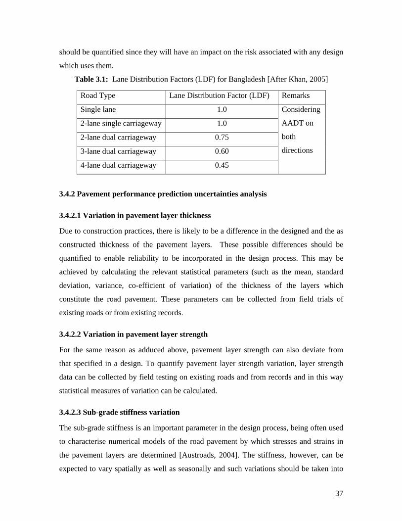
should be quantified since they will have an impact on the risk associated with any design
which uses them.
Table 3.1: Lane Distribution Factors (LDF) for Bangladesh [After Khan, 2005]
ctor (LDF) Remarks Road Type Lane Distribution Fa
Single lane 1.0
2-lane single carriageway 1.0
2-lane dual carriageway 0.75
3-lane dual carriageway 0.60
4-lane dual carriageway 0.45
Considering
AADT on
both
directions
3.4.2 Pavement performance prediction uncertainties analysis
3.4.2.1 Variation in pavement layer thickness
Due to construction practices, there is likely to be a difference in the designed and the as
constructed thickness of the pavement layers. These possible differences should be
quantified to enable reliability to be incorporated in the design process. This may be
achieved by calculating the relevant statistical parameters (such as the mean, standard
deviation, varian hich
constitute the road pavement. Th d trials of
existing roads or from existing records.
3.4.2.2 Variation in pavement layer strength
For the same reason as adduced above, paveme er strength can ate from
that specified in a design. To quantify pavemen r strength variation, layer strength
field testing on existing roads and from records and in this way
expected to vary spatially as well as seasonally and such variations should be taken into
ce, co-efficient of variation) of the thickness of the layers w
ese parameters can be collecte from field
nt lay also devi
t laye
data can be collected by
statistical measures of variation can be calculated.
3.4.2.3 Sub-grade stiffness variation
The sub-grade stiffness is an important parameter in the design process, being often used
to characterise numerical models of the road pavement by which stresses and strains in
the pavement layers are determined [Austroads, 2004]. The stiffness, however, can be
37
account in any reliability-based approach to pavement design. Usually this may be
achieved by determining statistical parameters such as the co-efficient of variation of sub-
grade stiffness for the length of the new road and, if possible, the associated seasonal
variation.
3.5 Embankment design data variability analysis
similar to that for determining the
reliability of road pavement design, as discussed above. Namely, the potential variability
ing standard statistical techniques and these
risk and reliability due to data uncertainty in other branches of engineering.
ber of criteria
were used, as follows:
method for its conditions is also an important criterion which includes the
following:
Uncertainty in the embankment design system, as identified in section 2.4, generally
results from variability in geometry, load, soil strength parameters, sub-soil properties
and consolidation factors. To quantify the risk and reliability, these uncertainties must be
evaluated. The procedure for achieving this is
of each of the parameters can be calculated us
measures of variability can then be used in an appropriate method to determine reliability.
3.6 Design risk quantification and reliability integration
To quantify the risk associated with design data variability and to incorporate reliability
in a design system for Bangladesh, the research investigates the various methods of risk
quantification and the processes available in the literature of incorporating reliability in
pavement and embankment design. In addition, the research also studies the process of
determining
To identify or to develop the most suitable methods for Bangladesh, a num
1. Accuracy: Any method selected must accurately determine risk and reliability.
2. Suitability for use in the proposed design system: The main goal of the research
project is to develop a comprehensive design system for Bangladesh.
Consequently, it is important that any method chosen should be suitable for the
design process being developed for the country.
3. Appropriateness for the conditions in Bangladesh: As the pavement design
system being developed will be used in Bangladesh, the appropriateness of the
38

a) Suitability for use with the data available in Bangladesh: that is, the methods
le computational procedure: Given the socio-economic conditions
.
pectively. The most appropriate techniques identified are used in the
logic
discu are used to validate the
su
3.7 O
Given the ultim
procedure to com the reliability of
em
3.8 Q
consistent.
3. It should be convenient to measure and quantify.
should make use of the data available in Bangladesh.
b) In accordance with the prevailing distress mode in Bangladesh: Reliability is
closely related to the predominant pavement distress modes. Thus a method
incorporating reliability should be selected such that it addresses the prevailing
pavement distress modes found in Bangladesh. For example, wheel track rutting is
not seen in Bangladesh, but cracking is common.
c) Requiring simp
in Bangladesh, procedures which are less rigorous will suit the country better.
4. Consider all the uncertainties in pavement design: The area of uncertainties in
pavement and embankment design was identified in section 2.4. A proper method
of incorporating reliability in the pavement and embankment design system of
Bangladesh should address all these uncertainties
A detailed description of the various methods of incorporating reliability found in the
literature is presented in the literature review chapter and a discussion of their relative
merits with respect to the above criteria is given in Chapters 5 and 6 for pavements and
embankments res
al design of a system to determine design reliability for Bangladesh and this is also
ssed in these two chapters. Finally, field testing data
ggested or developed method; these are presented in Chapter 7.
verall risk and reliability
ate objective of this research project, the study seeks to develop a
bine the reliability of pavement design and
bankment design. The way in which this was achieved is presented in Chapter 6.
uality control and quality assurance
Weed [2006] suggests that a criterion which can be used to measure the quality of
construction should meet the three following requirements:
1. It should be clearly related to performance.
2. Its performance relationship should be
39

In addition to these, a quality control process for the design system of Bangladesh must
satisfy the following:
1. It should be suitable for the design system of Bangladesh
2. It should be easy to understand and implement.
3. It should be convenient to measure and quantify
Different organizations and manufacturers follow different approaches for the quality
control of their materials and products. The prevailing quality control processes in
pavement and embankment construction, as found in the literature, are studied in this
ding their suitability and adaptability for Bangladesh
l parameters to quantify the
variab nts and embankments in
Bangladesh ncorporated in risk
assessm , respectively. The
arison of a number of techniques which may be used to construct
these t ntified for a
procedur purposes. A suitable
method for m d fully in Chapters 8
research and briefly discussed, inclu
in Chapters 8 and 9 respectively. The most appropriate techniques identified are used in
the logical design of a system for the quality control of pavement and embankment
construction in Bangladesh; this is also discussed in these chapters respectively.
3.9 Summary
The methods of analyzing data variability used in the present research have been
discussed in this chapter. The most appropriate statistica
ility of data used for the design of road paveme
were identified from the literature. These are to be i
ent tools for analytical pavement and embankment design
components and requirements for such tools were identified and described in this chapter,
whilst a detailed comp
ools is given in Chapters 5 and 6. Finally, the requirements were ide
e which can be used for quality control and assurance
eeting these requirements for Bangladesh is describe
and 9 with reference to pavements and embankments, respectively.
40
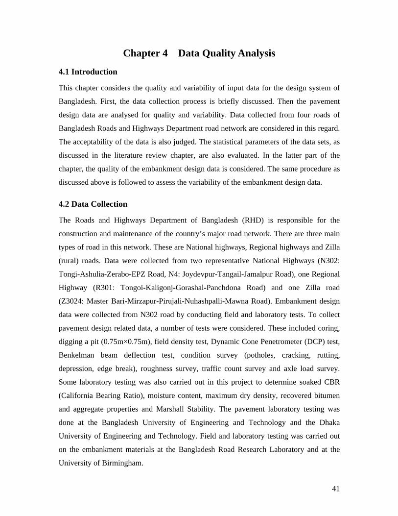
Chapter 4 Data Quality Analysis
he Roads and Highways Department of Bangladesh (RHD) is responsible for the
onstruction and maintenance of the country’s major road network. There are three main
types of road in this highways and Zilla
(rural) roads. Data were co ighways (N302:
o-EPZ Road, N4: Joydevpur-Tangail-Jamalpur Road), one Regional
BR
(California Bearing Ratio), moisture content, maximum dry density, recovered bitumen
es and Marshall Stability. The pavement laboratory testing was
4.1 Introduction
This chapter considers the quality and variability of input data for the design system of
Bangladesh. First, the data collection process is briefly discussed. Then the pavement
design data are analysed for quality and variability. Data collected from four roads of
Bangladesh Roads and Highways Department road network are considered in this regard.
The acceptability of the data is also judged. The statistical parameters of the data sets, as
discussed in the literature review chapter, are also evaluated. In the latter part of the
chapter, the quality of the embankment design data is considered. The same procedure as
discussed above is followed to assess the variability of the embankment design data.
4.2 Data Collection
T
c
network. These are National highways, Regional
llected from two representative National H
Tongi-Ashulia-Zerab
Highway (R301: Tongoi-Kaligonj-Gorashal-Panchdona Road) and one Zilla road
(Z3024: Master Bari-Mirzapur-Pirujali-Nuhashpalli-Mawna Road). Embankment design
data were collected from N302 road by conducting field and laboratory tests. To collect
pavement design related data, a number of tests were considered. These included coring,
digging a pit (0.75m×0.75m), field density test, Dynamic Cone Penetrometer (DCP) test,
Benkelman beam deflection test, condition survey (potholes, cracking, rutting,
depression, edge break), roughness survey, traffic count survey and axle load survey.
Some laboratory testing was also carried out in this project to determine soaked C
and aggregate properti
done at the Bangladesh University of Engineering and Technology and the Dhaka
University of Engineering and Technology. Field and laboratory testing was carried out
on the embankment materials at the Bangladesh Road Research Laboratory and at the
University of Birmingham.
41
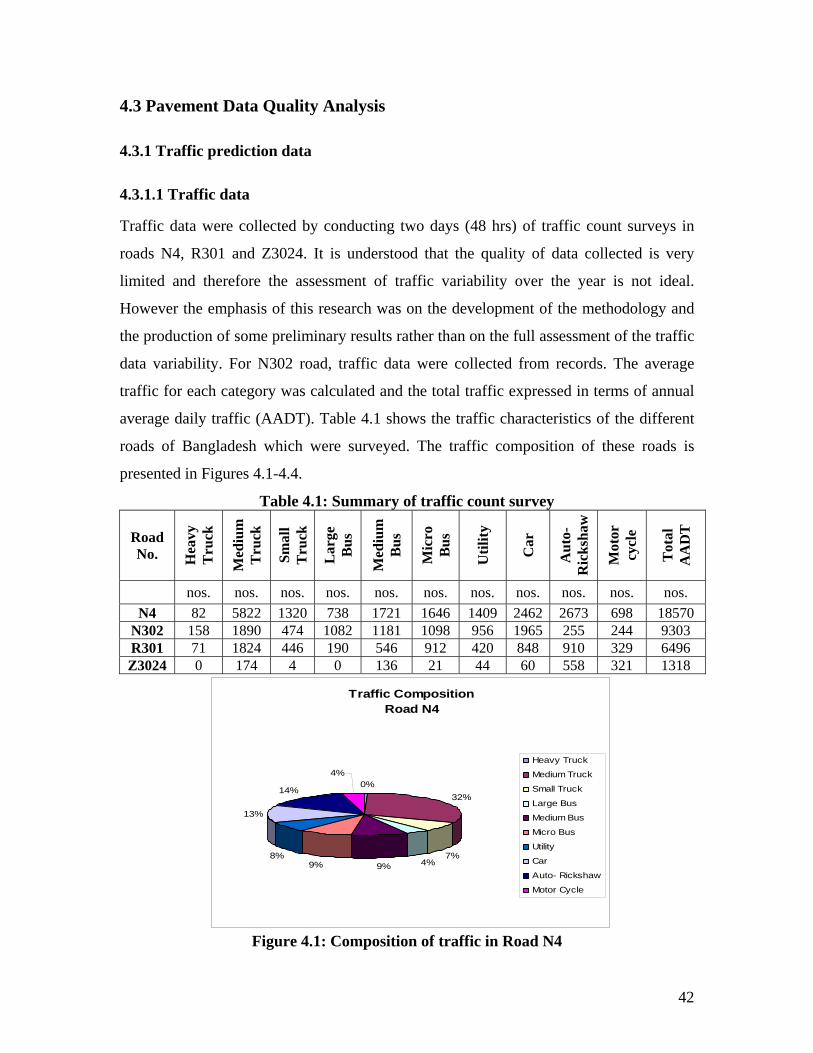
4.3 Pavement Data Quality Analysis
4.3.1 Traffic prediction data
4.3.1.1 Traffic data
Traffic data were collected by conducting two days (48 hrs) of traffic count surveys in
roads N4, R301 and Z3024. It is understood that the quality of data collected is very
limited and therefore the assessment of traffic variability over the year is not ideal.
However the emphasis of this research was on the development of the methodology and
the production of some preliminary results rather than on the full assessment of the traffic
data variability. For N302 road, traffic data were collected from records. The average
traffic for each category was calculated and the total traffic expressed in terms of annual
average daily traffic (AADT). Table 4.1 shows the traffic characteristics of the different
roads of Bangladesh which were surveyed. The traffic composition of these roads is
presented in Figures 4.1-4.4.
Table 4.1: Summary of traffic count survey
No. B Mic
ro
Bus
Util
ity
Car
Aut
o-
Ric
ksha
w
Mot
or
cy
cle
Tot
al
AA
DT
Road
Hea
vy
Tru
ck
Med
ium
T
ruck
Smal
l T
ruck
Lar
ge
Bus
Med
ium
us
nos. nos. nos. nos. nos. nos. nos. nos. nos. nos. nos. N4 82 5822 1320 738 1721 1646 1409 2462 2673 698 18570
N302 158 1890 474 1082 1181 1098 956 1965 255 244 9303 R301 71 1824 446 190 546 912 420 848 910 329 6496 Z3024 0 174 4 0 136 21 44 60 558 321 1318
Traffic CompositionRoad N4
0%32%
7%4%9%9%
8%
13%
14%
4%Heavy Truck
Medium Truck
Small Truck
Large Bus
Medium Bus
Micro Bus
Utility
Car
Auto- Rickshaw
Motor Cycle
F igure 4.1: Composition of traffic in Road N4
42
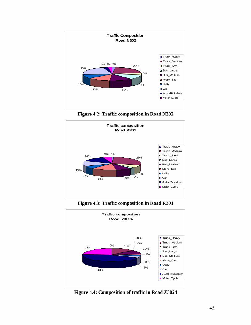
Tra m nN
2
5
12%
13%12%
10%
%
fficR
Cooad
po30
sitio2
% 20%
%
203% 3%
Truck_Heavy
Truck_Medium
Truck_Small
Bus_Large
Bus_Medium
Micro_Bus
Utility
Car
Auto-Rickshaw
Motor Cycle
Figure 4.2: Traffic composition in Road N302
Traffic compositionRoad R301
1%29%
7%3%8%14%
6%
13%
14%5%
Truck_Heavy
Truck_Medium
Truck_Small
Bus_Large
Bus_Medium
Micro_Bus
Utility
Car
Auto-Rickshaw
Motor Cycle
Figure 4.3: Traffic composition in Road R301
Traffic compositionRoad Z3024
0% 13%
0%
0%
Truck_Heavy
Truck_Medium
Truck_Small
Bus_Larg10%24%
e2%
3%
5%43%
Bus_Medium
Micro_Bus
Utility
Car
Auto-Rickshaw
Motor Cycle
Figure 4.4: Composition of traffic in Road Z3024
43
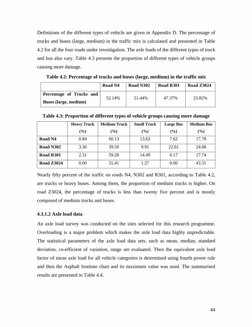
Definitions of the different types of vehicle are given in Appendix D. The percentage of
trucks and buses (large, medium) in the traffic mix is calculated and presented in Table
4.2 for all the four roads under investigation. The axle loads of the different types of truck
and bus also vary. Table 4.3 presents the proportion of different types of vehicle groups
causing more damage.
Table 4.2: Percentage of trucks and buses (large, medium) in the traffic mix
Road N4 Road N302 Road R301 Road Z3024
Percentage of Trucks and
Buses (large, medium) 52.14% 51.44% 47.37% 23.82%
Table 4.3: Propo g more damage
Heavy Truck
(%)
Medium Truck
(%)
Small Truck
(%)
Large Bus
(%)
Medium Bus
(%)
rtion of different types of vehicle groups causin
Road N4 0.84 60.13 13.63 7.62 17.78
Road N302 3.30 39.50 9.91 22.61 24.68
Road R301 2.31 59.28 14.49 6.17 17.74
Road Z3024 0.00 55.41 1.27 0.00 43.31
Nearly fifty percent of the traffic on roads N4, N302 and R301, according to Table 4.2,
are trucks or heavy buses. Among them, the proportion of medium trucks is higher. On
road Z3024, the percentage of trucks is less than twenty five percent and is mostly
composed of medi
the axle load data sets, such as mean, median, standard
evia
factor of mean axle load for all vehicle categories is determ
and then t and its maximum value was used. The summarised
results are p
um trucks and buses.
4.3.1.2 Axle load data
An axle load survey was conducted on the sites selected for this research programme.
Overloading is a major problem which makes the axle load data highly unpredictable.
The statistical parameters of
d tion, co-efficient of variation, range are evaluated. Then the equivalent axle load
ined using fourth power rule
the Asphalt Institute char
resented in Table 4.4.
44
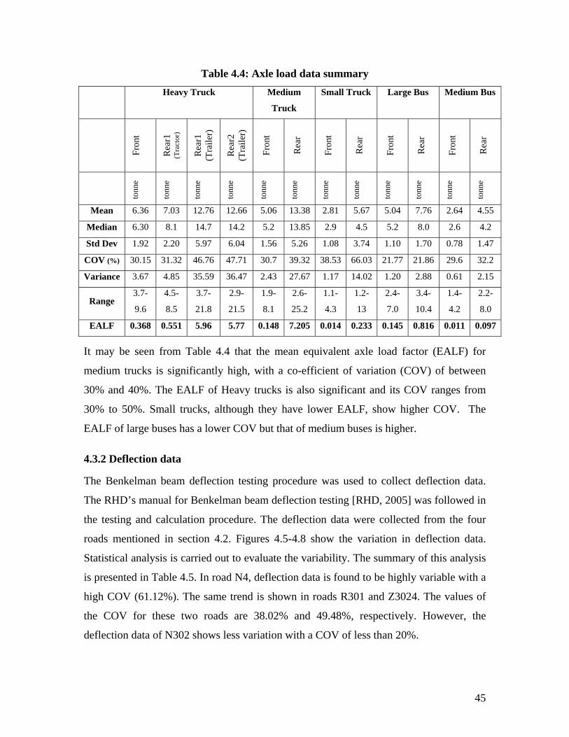
Table d ry
Heavy Truck l Truck e Bus m Bus
4.4: Axle loadMedium
ata summaSmal
Larg
Truck
Mediu
Rea
r1
(Tra
ctor
)
(Tra
iler)
Rea
r2
(Tra
iler)
Rea
r
Rea
r
Rea
r
Rea
r
Fron
t
Rea
r1
Fron
t
Fron
t
Fron
t
Fron
t
tonn
e
tonn
e
tonn
e
tonn
e
tonn
e
tonn
e
tonn
e
tonn
e
tonn
e
tonn
e
tonn
e
tonn
e
Mean 6.36 7.03 12.76 12.66 5.06 13.38 2.81 5.67 5.04 7.76 2.64 4.55
Median 6.30 8.1 14.7 14.2 5.2 13.85 2.9 4.5 5.2 8.0 2.6 4.2
Std Dev 1.92 2.20 5.97 6.04 1.56 5.26 1.08 3.74 1.10 1.70 0.78 1.47
COV (%) 30.15 31.32 46.76 47.71 30.7 39.32 38.53 66.03 21.77 21.86 29.6 32.2
Variance 3.67 4.85 35.59 36.47 2.43 27.67 1.17 14.02 1.20 2.88 0.61 2.15
Range 3.7-
9.6
4.5-
8.5
3.7-
21.8
2.9-
21.5
1.9-
8.1
2.6-
25.2
1.1-
4.3
1.2-
13
2.4-
7.0
3.4-
10.4
1.4-
4.2
2.2-
8.0
EALF 0.368 0.551 5.96 5.77 0.148 7.205 0.014 0.233 0.145 0.816 0.011 0.097
It may be seen from Table 4.4 that the mean equivalent axle load factor (EALF) for
medium trucks is significantly high, with a co-efficient of variation (COV) of between
30% and 40%. The EALF of Heavy trucks is also significant and its COV ranges from
30% to 50%. Small trucks, although they have lower EALF, show higher COV. The
ALF of large buses has a lower COV but that of medium buses is higher.
.3.2 Deflection data
an bea ure was used to coll
The RHD’s manual for Benkelman beam ion testing [RHD, 2005] was followed in
e testing and calculation procedure. The deflection data were collected from the four
roads mentioned in section 4.2. Figures 4.5- sh the riat in lec da
Statistical analysis is carried out to evaluate the variability. The summary of this analysis
presente n T 4 ro 4, ect dat fou o b gh ria wi
high COV 1.1 . T am nd how n ro s R an 302 he ues
the COV for these two roads are 38.02%
w C f th %
E
4
The Benkelm m deflection testing proced ect deflection data.
deflect
th
4.8 ow va ion def tion ta.
is d i
(6
able
2%)
.5. In
he s
ad N
e tre
defl
is s
ion
n i
a is
ad
nd t
301
e hi
d Z
ly va
4. T
ble
val
th a
of
and 49.48%, respectively. However, the
deflection data of N302 shows less variation ith a OV o less an 20 .
45
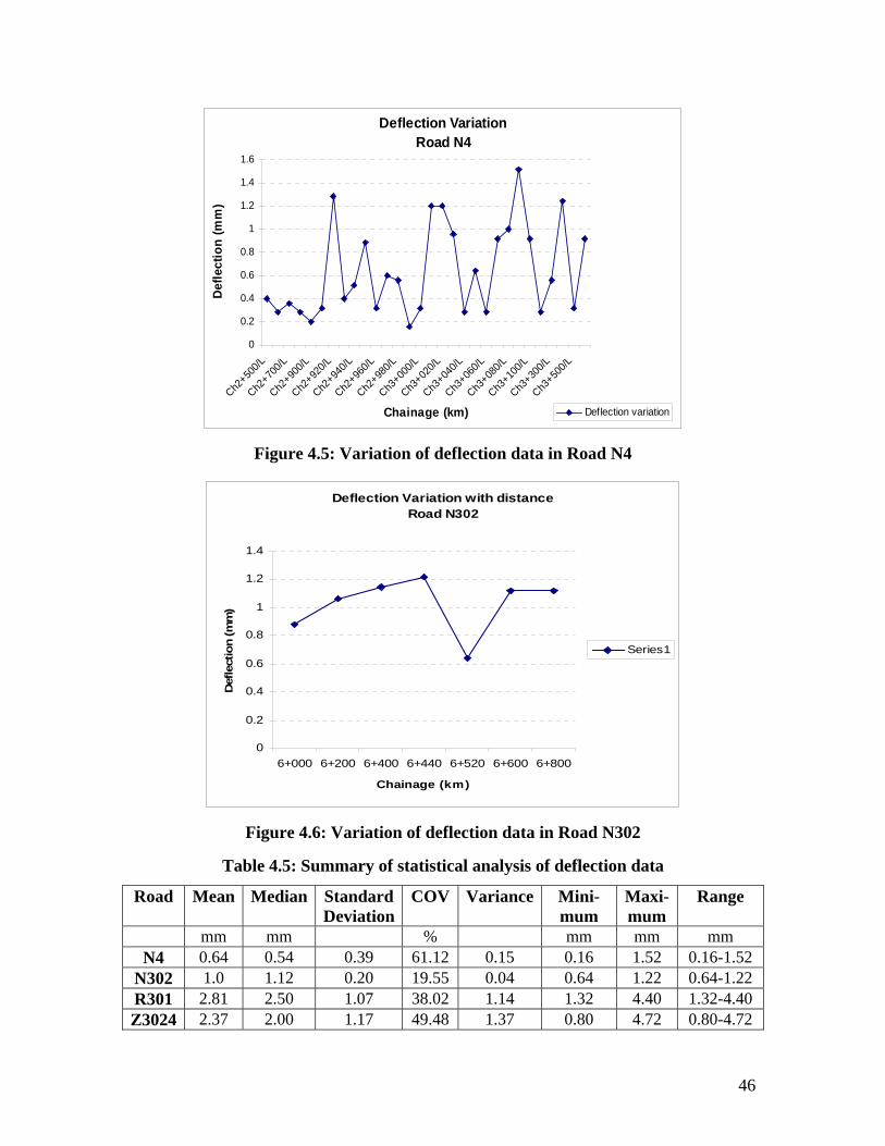
Deflection VariationRoad
1.2
1.
1.6
500/L
700/L
900/L
h2+92
0/L
Ch2+94
0/L
Ch2+96
0/L
Ch2+98
0/L
Ch3+00
0/L
Ch3+02
0/L
Ch3+04
0/L
Ch3+06
0/L
Ch3+08
0/L
Ch3+10
0/L
Ch3+30
0/L
Ch3+50
0/L
Chainage (km)
)
N4
4
0
0.2
0.4
0.6
0.8
1De
flect
ion
(mm
Ch2+
Ch2+
Ch2+
C
Deflection variation
Figure 4.5: Variation of deflection data in Road N4
Deflection Variation with distance Road N302
0.6
0.8
1
1.2
1.4
efle
ctio
n (m
m)
0
0.2
0.4
6+000 6+200 6+400 6+440 6+520 6+600 6+800
Chainage (km)
D
Series1
Figure 4.6: Variation of deflection data in Road N302
Table 4.5: Summary of statistical analysis of deflection data
Road Mean Median Standard Deviation
COV Variance Mini-mum
Maxi-mum
Range
mm mm % mm mm mm N4 0.64 0.54 0.39 61.12 0.15 0.16 1.52 0.16-1.52
N302 1.0 1.12 0.20 19.55 0.04 0.64 1.22 0.64-1.22 R301 2.81 2.50 1.07 38.02 1.14 1.32 4.40 1.32-4.40 Z3024 2.37 2.00 1.17 49.48 1.37 0.80 4.72 0.80-4.72
46
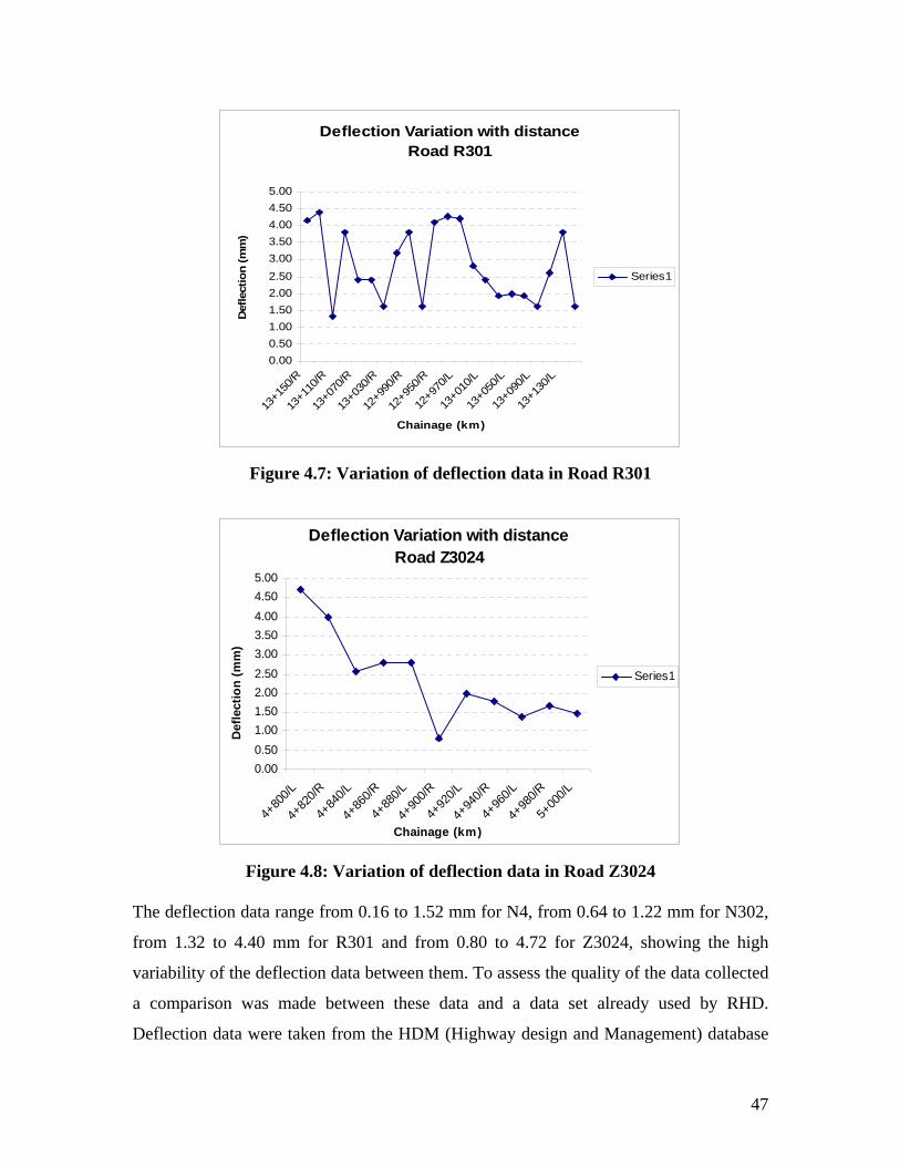
Deflection Variation with distance Road R301
0.000.501.001.502.002.503.003.504.004.505.00
13+15
0/R
13+11
0/R
13+07
0/R
13+03
0/R
12+99
0/R
12+95
0/R
12+97
0/L
13+01
0/L
13+05
0/L
13+09
0/L
13+13
0/L
Chainage (km)
Def
lect
ion
(mm
)
Series1
F
igure 4.7: Variation of de lection data in Road R301f
Deflection Variation with distance Road Z3024
0.000.501.001.502.002.503.003.504.004.505.00
4+80
0/L
4+82
0/R
4+84
0/L
4+86
0/R
4+88
0/L
4+90
0/R
4+92
0/L
4+94
0/R
4+96
0/L
4+98
0/R
5+00
0/L
Chainage (km)
Def
lect
ion
(mm
)
Series1
Figure 4.8: Variation of deflection data in Road Z3024
The defl a m om o for N302,
from 1.32 .40 for fr 80 to 4.72 for Z3024, showing the high
variability of the deflection da wee e y of ata
ar was e bet the and a data set alread d
o we en fro HD ghw esign ana nt) database
ection d ta range from 0.16 to
R30 and
1.52 m for N4, fr 0.64 t 1.22 mm
to 4 mm 1 om 0.
ta bet n them. To assess th qualit the d collected
a comp ison mad ween se data y use by RHD.
Deflecti n data re tak m the M (Hi ay d and M geme
47
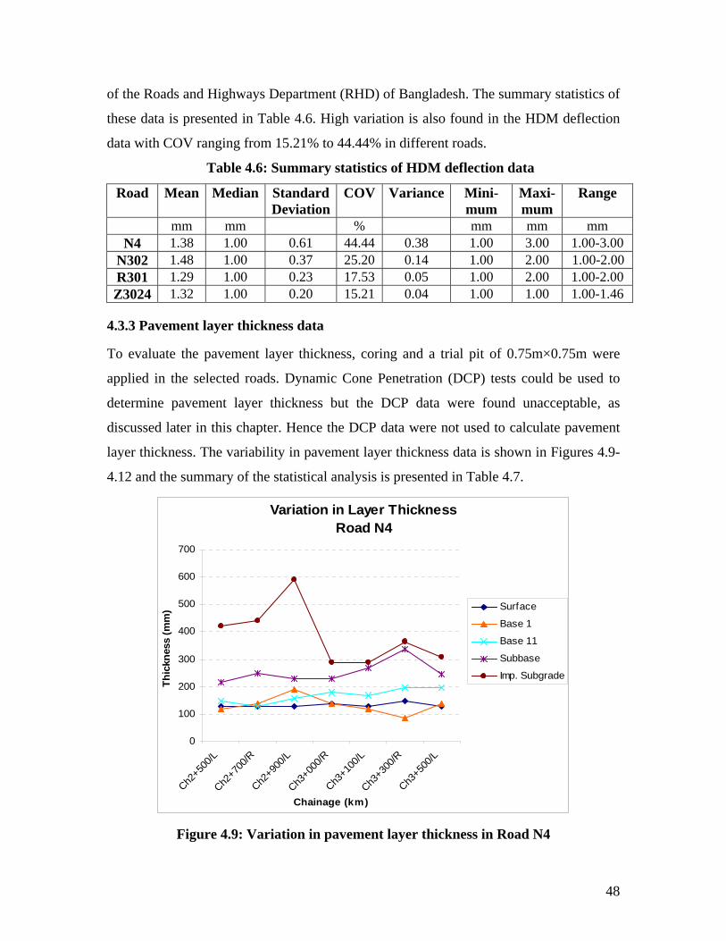
of the Roads and Highways Department (RHD) of Bangladesh. The summary statistics of
these data is presented in Table 4.6. High variation is also found in the HDM deflection
data with COV ranging from 15.21% to 44.44% in different roads.
Table 4.6: Summary statistics of HDM deflection data
Road Mean Median Standard Deviation
COV Variance Mini-mum
Maxi-mum
Range
mm mm % mm mm mm N4 1.38 1.00 0.61 44.44 0.38 1.00 3.00 1.00-3.00
N302 1.48 1.00 0.37 25.20 0.14 1.00 2.00 1.00-2.00 R301 1.29 1.00 0.23 17.53 0.05 1.00 2.00 1.00-2.00 Z3024 1.32 1.00 0.20 15.21 0.04 1.00 1.00 1.00-1.46
4.3.3 Pavement layer thickness data
To evaluate the pavement layer thickness, coring and a trial pit of 0.75m× were
applied in the s uld be used to
determine pavement layer thickness but t e DCP data were found unacceptable, as
discussed later in this chapter. Hence the DCP data were not used to calculate pavement
layer thickness. The variability in pavement layer thickness data is shown in Figures 4.9-
4.12 and the summary of the statistical analysis is presented in Table 4.7.
0.75m
elected roads. Dynamic Cone Penetration (DCP) tests co
h
Variation in Layer ThicknessRoad N4
100
200
300
400
500
600
700
Thic
knes
s (m
m) Surface
Base 1
Base 11
Subbase
Imp. Subgrade
0
Ch2+50
0/L
Ch2+70
0/R
Ch2+90
0/L
Ch3+00
0/R
Ch3+10
0/L
Ch3+30
0/R
Ch3+50
0/L
Chainage (km)
Figure 4.9: Variation in pavement layer thickness in Road N4
48
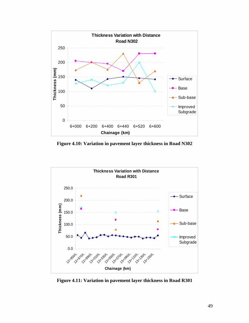
Thickness Variation with Distance Road N302
250
50
ess
(mm
100
150
200
Thic
kn)
S eurfac
Base
S seub-ba
ImprovedSubgrade
06+000 6+200 6+400 6+440 6+520 6+600
Chainage (km)
Figure 4.10: Variation in pavement layer thickness in Road N302
Thickness Variation with DistanceRoad R301
0.0
50.0
100.0
150.0
200.0
250.0
12+95
0/L
12+97
0/L
12+99
0/L
13+01
0/L
13+03
0/L
13+05
0/L
13+07
0/L
13+09
0/L
13+11
0/L
13+13
0/L
13+15
0/L
Chainage (km)
Thic
knes
s (m
m)
Surface
Base
Sub-base
ImprovedSubgrade
Figure 4.11: Variation in pavement layer thickness in Road R301
49
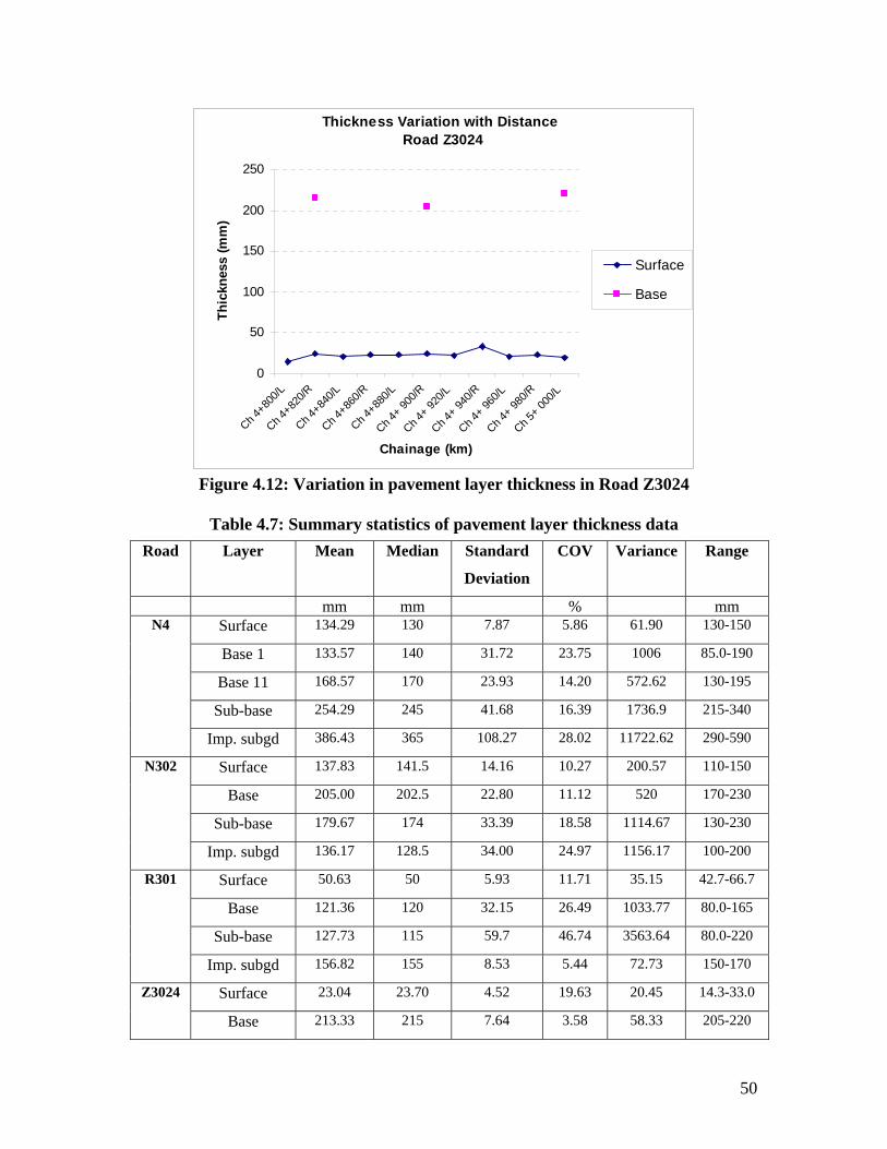
Thickness Variation with Distance Road Z3024
0
50
100
150
200
250
Ch 4+80
0/L
Ch 4+82
0/R
Ch 4+84
0/L
Ch 4+86
0/R
Ch 4+88
0/L
Ch 4+ 90
0/R
Ch 4+ 92
0/L
Ch 4+ 94
0/R
Ch 4+ 96
0/L
Ch 4+ 98
0/R
Ch 5+ 00
0/L
Chainage (km)
Thic
knes
s (m
m)
Surface
Base
Figure 4.12: Variation in pavement layer thickness in Road Z3024
Road Layer Mean Median Standard
Deviation
COV Variance Range Table 4.7: Summary statistics of pavement layer thickness data
mm mm % mm Surface 134.29 130 7.87 5.86 61.90 130-150
Base 1 133.57 140 31.72 23.75 1006 85.0-190
Base 11 168.57 170 23.93 14.20 572.62 130-195
Sub-base 254.29 245 41.68 16.39 1736.9 215-340
N4
Imp. subgd 386.43 365 108.27 28.02 11722.62 290-590
Surface 137.83 141.5 14.16 10.27 200.57 110-150
Base 205.00 202.5 22.80 11.12 520 170-230
Sub-base 179.67 174 33.39 18.58 1114.67 130-230
N302
Imp. subgd 136.17 128.5 34.00 24.97 1156.17 100-200
Surface 50.63 50 5.93 11.71 35.15 42.7-66.7
Base 121.36 120 32.15 26.49 1033.77 80.0-165
Sub-base 127.73 115 59.7 46.74 3563.64 80.0-220
R301
Imp. subgd 156.82 155 8.53 5.44 72.73 1 -170 50
Surface 23.04 23.70 4.52 19.63 20.45 14.3-33.0 Z3024
Base 213.33 215 7.64 3.58 58.33 205-220
50
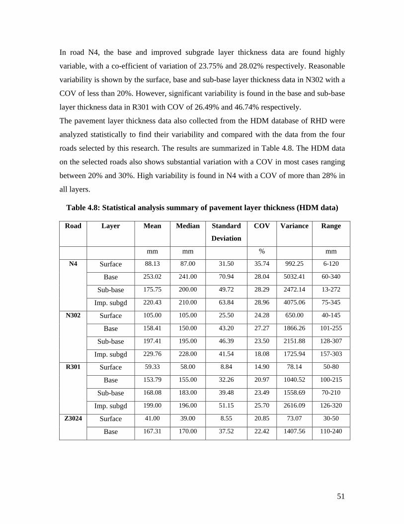
In road N4, the base and improved subgrade layer thickness data are found highly
variable, with a co-efficient of variation of 23.75% and 28.02% respectively. Reasonable
variability is shown by the surface, base and sub-base layer thickness data in N302 with a
COV of less than 20%. However, significant variability is found in the base and sub-base
layer thickness data in R301 with COV of 26.49% and 46.74% respectively.
The pavement layer thickness data also collected from the HDM database of RHD were
analyzed statistically to find their variability and compared with the data from the four
roads selected by this research. The results are summarized in Table 4.8. The HDM data
on the selected roads also shows substantial variation with a COV in most cases ranging
between 20% and 30%. High variability is found in N4 with a COV of more than 28% in
all layers.
Table 4.8: Statistical analysis summary of pavement layer thickness (HDM data)
Road Range
Layer Mean Median Standard COV Variance
Deviation
mm mm % mm
Surface 88.13 87.00 35.74 992.25 6-120 31.50
Base 2 2 70 4 2 503 41 6 53.02 41.00 .9 8.04 2. 0-340
Sub-base 175.75 200.00 49 28 24.72 .29 72.14 13-272
N4
Im 2 4
p. subgd 220.43 10.00 63.84 28.96 075.06 75-345
Surface 105.00 105.00 25.50 24.28 650.00 40-145
Base 158.41 1 50.00 43.20 27.27 1866.26 101-255
Sub-base 197.41 195.00 46.39 23.50 2151.88 128-307
N302
Im p. subgd 229.76 228.00 41.54 18.08 1725.94 157-303
Surface 7859.33 58.00 8.84 14.90 .14 50-80
Base 153.79 155.00 32.26 20.97 1040.52 100-215
Sub-base 168.08 183.00 39.48 23.49 1558.69 70-210
R301
Im 19 19 0 51 26p. subgd 9.00 6.0 .15 25.70 16.09 126-320
41.00 39.00 8.55 20.85 73.07 30-50 Surface Z3024
37Base 167.31 170.00 .52 22.42 1407.56 110-240
51
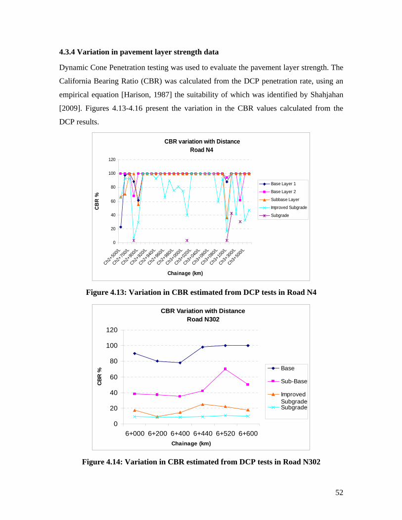
4.3.4 Variation in pavement layer strength data
Dynamic Cone Penetration testing was used to evaluate the pavement layer strength. The
California Bearing Ratio (CBR) was calculated from the DCP penetration rate, using an
empirical equation [Harison, 1987] the suitability of which was identified by Shahjahan
[2009]. Figures 4.13-4.16 present the variation in the CBR values calculated from the
DCP results.
CBR variation with DistanceRoad N4
100
120
Base Layer 1
0
40
80
/L70
0/L
+900/L
Ch2+92
0/L
Ch298
0/L
Ch3+00
0/L
Ch306
0/L
Ch3+08
0/L
Ch3+10
0/L 0/L 00/L
Cha )
R %
Base Layer 2
Subbase Layer
Improved Subgrade60
CB
Subgrade
20
Ch2+
Ch2+
Ch250
0+
Ch2+9
Ch2+94
0/L 60/L
+Ch3
+0Ch3
+020/L 40
/L
Ch3+3
Ch3+50
inage (km
Figure 4.13: Variation in CBR estimated from DCP tests in Road N4
CBR n with ceRoad N302
6+000 6+200 6+400 6+440 6+520 6+600Chainage (km)
CBR
%
Variatio Distan
0
20
40
60
80
100
120
Base
Sub-Base
ImprovedSubgradeSubgrade
Figure 4.14: Variation in CBR estimated from DCP tests in Road N302
52
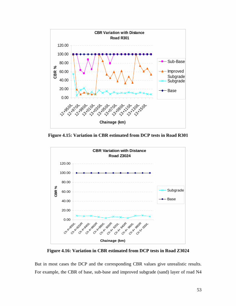
CBR Variation with Distance
0.00
20.00
40.00
0.00
12+9
50/L
12+9
70/L
12+9
90/L
13+0
10/L
13+0
30/L
13+0
50/L
13+0
70/L
13+0
90/L
13+1
10/L
13+1
30/L
13+1
50/L
Chainage (km)
CB
Road R301
6
80.00
100.00
120.00
R %
Sub-Base
ImprovedSubgradeSubgrade
Base
Figure 4.15: Variation in CBR estimated from DCP tests in Road R301
CBR Variation with DistanceRoad Z3024
0.00
20.00
40.00
60.00
80.00
100.00
120.00
Ch 4+80
0/L
Ch 4+82
0/R
Ch 4+84
0/L
Ch 4+86
0/R
Ch 4+88
0/L
Ch 4+ 90
0/R
Ch 4+ 92
0/L
Ch 4+ 94
0/R
Ch 4+ 96
0/L
Ch 4+ 98
0/R
Ch 5+ 00
0/L
Chainage (km)
CBR
% Subgrade
Base
Figure 4.16: Variation in CBR estimated from DCP tests in Road Z3024
But in most cases the DCP and the corresponding CBR values give unrealistic results.
For ex ad N4 ample, the CBR of base, sub-base and improved subgrade (sand) layer of ro
53
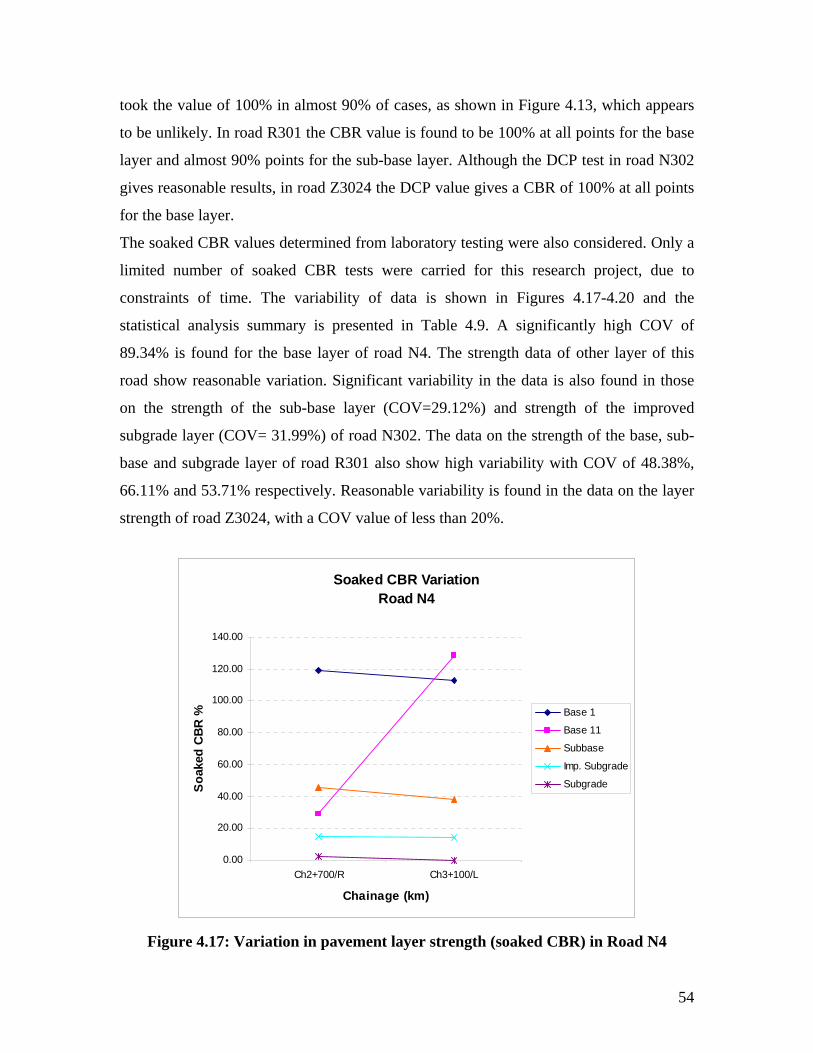
took the value of 100% in almost 90% of cases, as shown in Figure 4.13, which appears
to be unlikely. In road R301 the CBR value is found to be 100% at all points for the base
layer and almost 90% points for the sub-base layer. Although the DCP test in road N302
gives reasonable results, in road Z3024 the DCP value gives a CBR of 100% at all points
for the base layer.
The soaked CBR values determined from laboratory testing were also considered. Only a
limited number of soaked CBR tests were carried for this research project, due to
constraints of time. The variability of data is shown in Figures 4.17-4.20 and the
statistical analysis summary is presented in Table 4.9. A significantly high COV of
89.34% is found for the base layer of road N4. The strength data of other layer of this
road show reasonable variation. Significant variability in the data is also found in those
on the strength of the sub-base layer (COV=29.12%) and strength of the improved
subgrade layer (COV= 31.99%) of road N302. The data on the strength of the base, sub-
base an .38%,
66.11% and 53.71% respectively. Reasonable variability is found in the data on the layer
strength of road Z3024, with a COV value of less than 20%.
d subgrade layer of road R301 also show high variability with COV of 48
Soaked CBR VariationRoad N4
20.00
40.00
60.00
80.00
100.00
120.00
140.00
Soa
ked
CBR
% Base 1
Base 11
Subbase
Imp. Subgrade
Subgrade
0.00Ch2+700/R Ch3+100/L
Chainage ( m)k
Figure 4.17: Variation in pavement layer strength (soaked CBR) in Road N4
54
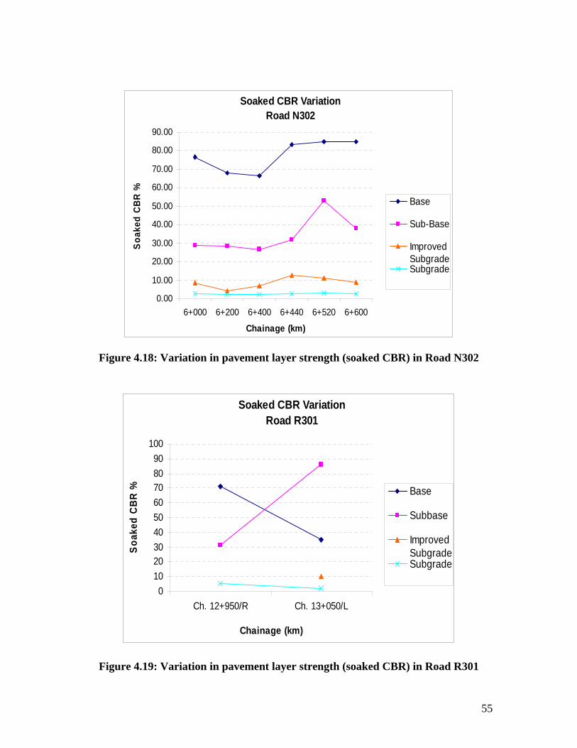
Soaked CBR Variation Road N302
80.00
90.00
0.00
10.00
20.00
30.00
40.00
50.00
60.00
70.00
6+000 6+200 6+400 6+440 6+520 6+600
Chainage (km)
Soa
ked
CBR
%
Base
Sub-Base
ImprovedSubgradeSubgrade
Figure 4.18: Variation in pavement layer strength (soaked CBR) in Road N302
Soaked CBR Variation Road R301
0102030405060708090
100
Ch. 12+950/R Ch. 13+050/L
Chainage (km)
Soa
ked
CBR
% Base
Subbase
ImprovedSubgradeSubgrade
F igure 4.19: Variation in pavement layer strength (soaked CBR) in Road R301
55
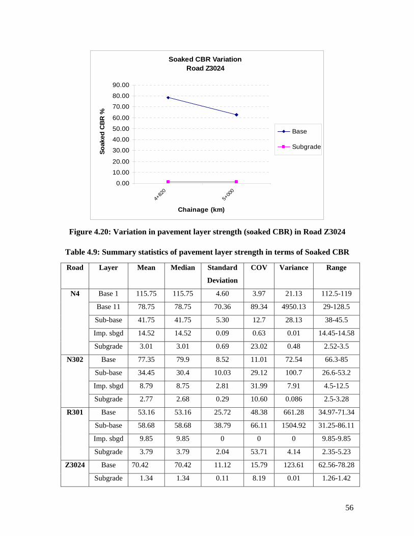
Soaked CBR Variation Road Z3024
0.00
10.00
20.00
30.00
40.00
50.00
60.00
70.00
80.00
90.00
4+82
05+
000
Chainage (km)
Soak
ed C
BR
%
Base
Subgrade
Figure 4.20: Variation in pavement layer strength (soaked CBR) in Road Z3024
T
Road Layer Mean Median tandard
Deviation
COV Variance Range
able 4.9: Summary statistics of pavement layer strength in terms of Soaked CBR
S
Base 1 115.75 115.75 4.60 3.97 21.13 112.5-119
Base 11 78.75 78.75 70.36 89.34 4950.13 29-128.5
Sub-base 41.75 41.75 5.30 12.7 28.13 38-45.5
Imp. sbgd 14.52 14.52 0.09 0.63 0.01 14.45-14.58
N4
Subgrade 3.01 3.01 0.69 23.02 0.48 2.52-3.5
Base 77.35 79.9 8.52 11.01 72.54 66.3-85
Sub-base 34.45 30.4 10.03 29.12 100.7 26.6-53.2
Imp. sbgd 8.79 8.75 2.81 31.99 7.91 4.5-12.5
N302
Subgrade 2.77 2.68 0.29 10.60 0.086 2.5-3.28
Base 53.16 53.16 25.72 48.38 661.28 34.97-71.34
Sub-base 58.68 58.68 38.79 66.11 1504.92 31.25-86.11
Imp. sbgd 9.85 9.85 0 0 0 9.85-9.85
R301
Subgrade 3.79 3.79 2.04 53.71 4.14 2.35-5.23
Base 70.42 70.42 11.12 15.79 123.61 62.56-78.28 Z3024
2 Subgrade 1.34 1.34 0.11 8.19 0.01 1.26-1.4
56
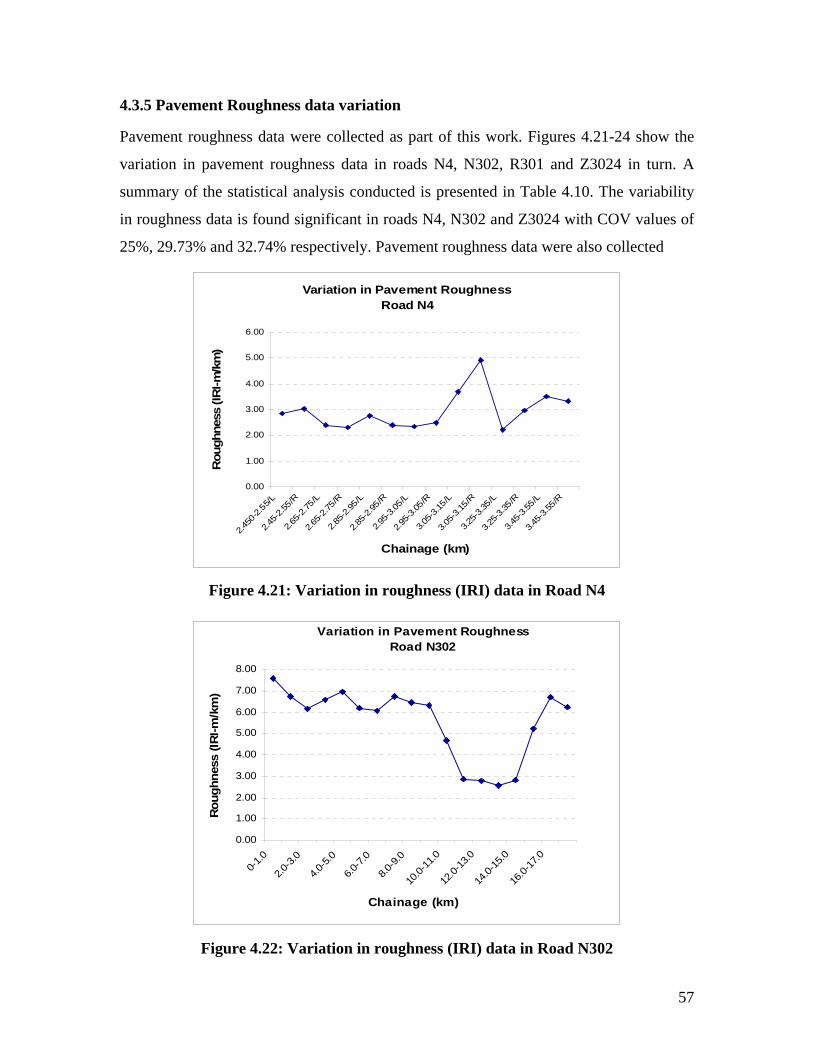
4.3.5 Pavement Roughness data variation
Pavement roughness data were collected as part of this work. Figures 4.21-24 show the
variation in pavement roughness data in roads N4, N302, R301 and Z3024 in turn. A
summary of the statistical analysis conducted is presented in Table 4.10. The variability
in roughness data is found significant in roads N4, N302 and Z3024 with COV values of
25%, 29.73% and 32.74% respectively. Pavement roughness data were also collected
Variation in Pavement RoughnessRoad N4
1.00Rou
0.00
55/L 5
2.00
3.00
4.00
5.00
6.00
450-
2.
2.4.
2.5-
22.6
5-2
2.65
5 .-2
.
2.
. . .
2.95
3. . . .
3.25
. .-3
./R
75/L
75/R
95/L
95/R
05/L
05/R
15/L
15/R
35/L
35/R
55/L
585
-2
2.85-
22.9
5-3 -
3.05-
3
3.05-
33.2
5-3 -3
3.45-
3
3.45
5
Cha
ghne
ss (I
RI-m
/km
)
/R
inage (km)
Figure 4.21: Variation in roughness (IRI) data in Road N4
Variation in Pave Roug Road
1.00
2.00
0
6.00
00
00
1.0
2 4.0-5
.0
6. 8.0-9
.0
10.0-
11.
.0-13
.0
14.0-
15.0
-17.0
ainage
ment hness N302
0.00
3.00
ghn
4.0
ess
(I
5.00
RI-m
7.
8.
0- .0-3.0
0-7.0
0
12 16.0
Ch (km)
Rou
/km
)
Figure 4.22 riatio oughn RI) d Roa 02 : Va n in r ess (I ata in d N3
57
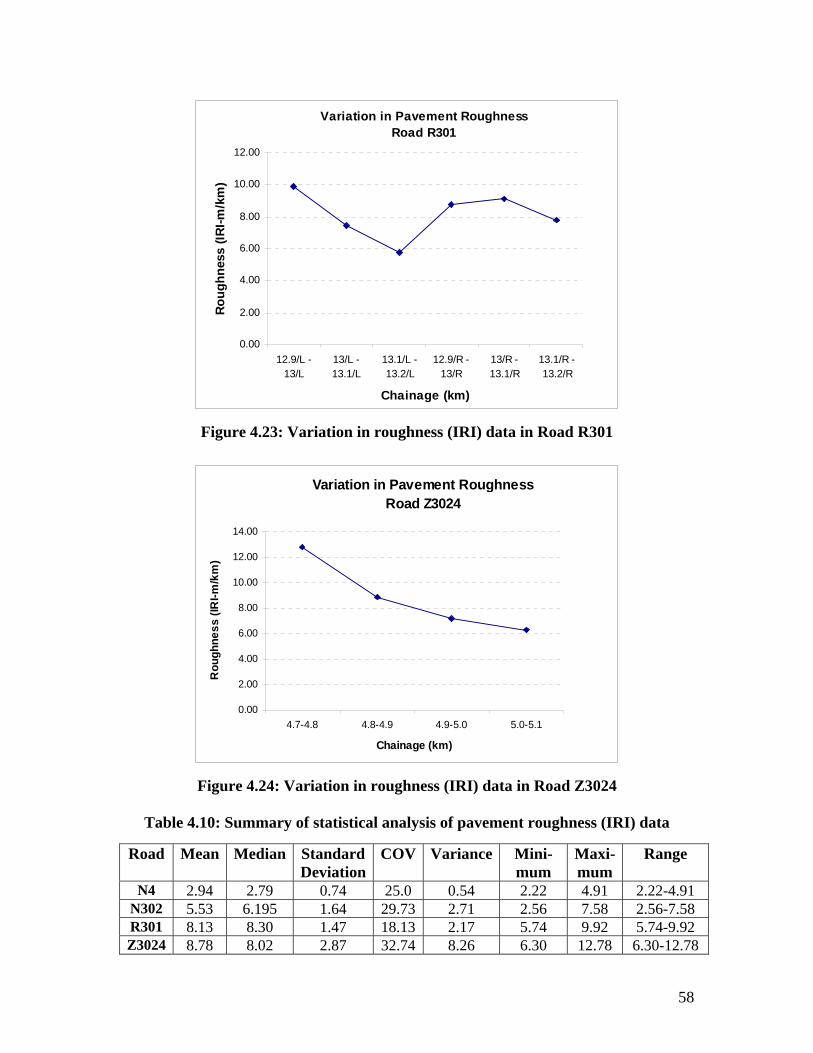
Variation in Pavement Roughness Road R301
6.00
8.00
10.00
12.00
ss (I
RI-m
/km
)
0.00
2.00
4.00
12.9/L -13/L
13/L -13.1/L
13.1/L -13.2/L
12.9/R -13/R
13/R -13.1/R
13.1/R -13.2/R
Chainage (km)
Roug
hne
Figure 4.23: Variation in roughness (IRI) data in Road R301
Variation in Pavement Roughness Road Z3024
0.00
2.00
4.00
6.00
8.00
10.00
I-m/k
12.00
14.00
4.7-4.8 4.8-4.9 4.9-5.0 5.0-5.1
Chainage (km)
Rou
ghne
ss (I
Rm
)
Figure 4.24: Variation in roughness (IRI) data in Road Z3024
Table 4.10: Summary of statistical analysis of pavement roughness (IRI) data
Road Mean Median Standard Deviation
COV Variance Mini-mum
Maxi-mum
Range
N4 2.94 2.79 0.74 25.0 0.54 2.22 4.91 2.22-4.91 N302 5.53 6.195 1.64 29.73 2.71 2.56 7.58 2.56-7.58 R301 8.13 8.30 1.47 18.13 2.17 5.74 9.92 5.74-9.92 Z3024 8. 6.30-12.78 78 8.02 2.87 32.74 8.26 6.30 12.78
58
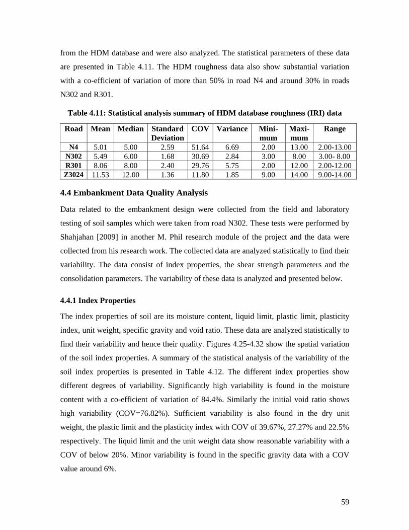
from the HDM database and were also analyzed. The statistical parameters of these data
are presented in Table 4.11. The HDM roughness data also show substantial variation
with a co-efficient of variation of more than 50% in road N4 and around 30% in roads
N302 and R301.
Table 4.11: Statistical analysis summary of HDM database roughness (IRI) data
Road Mean Median Standard Deviation
COV Variance Mini-mum
Maxi-mum
Range
N4 5.01 5.00 2.59 51.64 6.69 2.00 13.00 2.00-13.00 N302 5.49 6.00 1.68 30.69 2.84 3.00 8.00 3.00- 8.00 R301 8.06 8.00 2.40 29.76 5.75 2.00 12.00 2.00-12.00 Z3024 11.53 12.00 1.36 11.80 1.85 9.00 14.00 9.00-14.00
4.4 Embankment Data Quality Analysis
Data related to the embankment design were collected from the field and laboratory
testing of soil sam ed by
Shahjahan [2009] in another M. Phil research module of the project and the data were
collected from his research work. The collected data are analyzed statistically to find their
variability. The data consist of index properties, the shear strength parameters and the
consolidation parameters. The variability of these data is analyzed and presented below.
4.4.1 Index Properties
The index properties of soil are its moisture content, liquid limit, plastic limit, plasticity
index, unit weight, specific gravity and void ratio. These data are analyzed statistically to
find their variability and hence their quality. Figures 4.25-4.32 show the spatial variation
of the soil index properties. A summary of the statistical analysis of the variability of the
soil index properties is presented in Table 4.12. The different index properties show
different degrees of variability. Significantly high variability is found in the moisture
content wit atio shows
hig nit
w t i ty of , an
respectively. The liquid lim nit weight data show reasonabl ility with a
C b 20% or va ity d in pecifi ity wit
value around 6%.
ples which were taken from road N302. These tests were perform
h a co-efficient of variation of 84.4%. Similarly the initial void r
h variability (COV=76.82%). Sufficient variability is also found in the dry u
eight, he plast c limit and the plastici
it and the u
index with COV 39.67% 27.27%
e variab
d 22.5%
OV of elow . Min riabil is foun the s c grav data h a COV
59
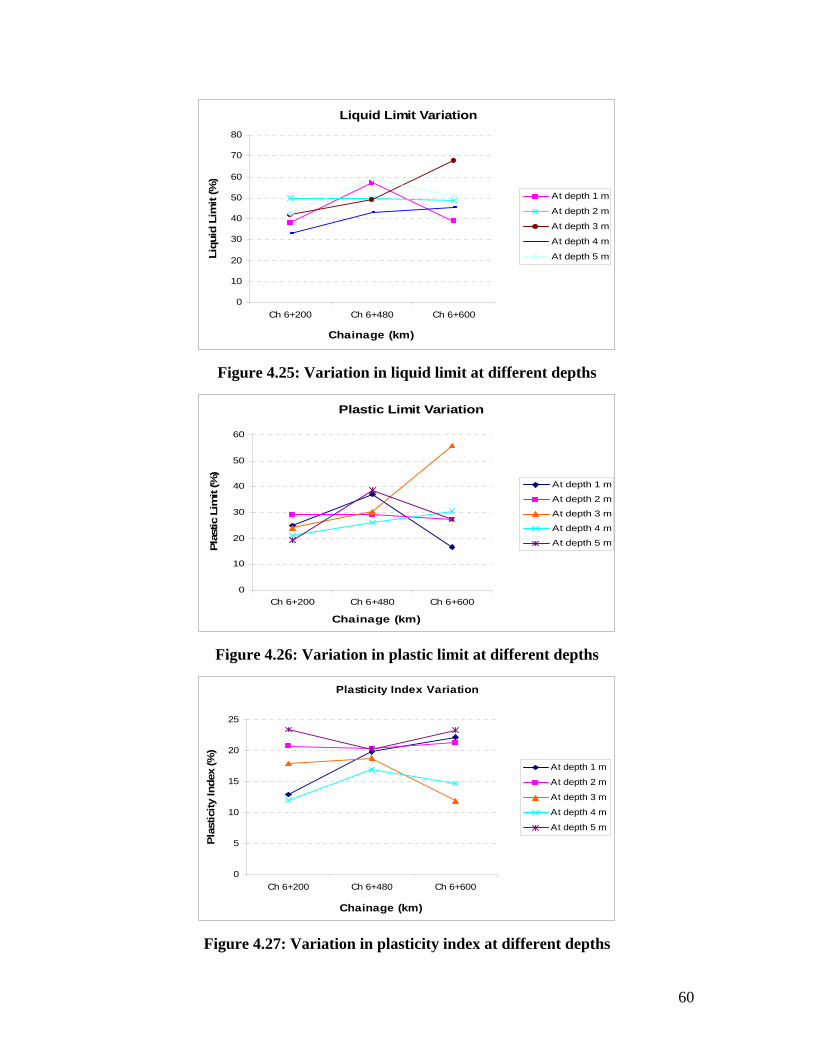
Liquid Limit Variation
0
10
20
30
50
60
70
80
t (%
)At depth 1 m
40d
Li
Ch 6+200 h 6+ Ch
nag
qui
mi
C 480 6+600
Chai e (km)
LiAt depth 2 m
At depth 3 m
At depth 4 m
At depth 5 m
d limit at different depths Figure 4.25: Variation in liqui
Plastic Limit Variation
10
20
30
40
50
60
Plas
tic L
imit
(%)
At depth 1 m
At depth 2 m
At depth 3 m
At depth 4 m
At depth 5 m
0Ch 6+200 Ch 6+480 Ch 6+600
Chainage (km)
Figure 4.26: Variation in plastic limit at different depths
Plasticity Index Variation
0
5
10
15
20
25
Ch 6+200 Ch 6+480 Ch 6+600
Chainage (km)
Plas
ticity
Inde
x (%
)
At depth 1 m
At depth 2 m
At depth 3 m
At depth 4 m
At depth 5 m
: Variation in plasticity index at different depths Figure 4.27
60
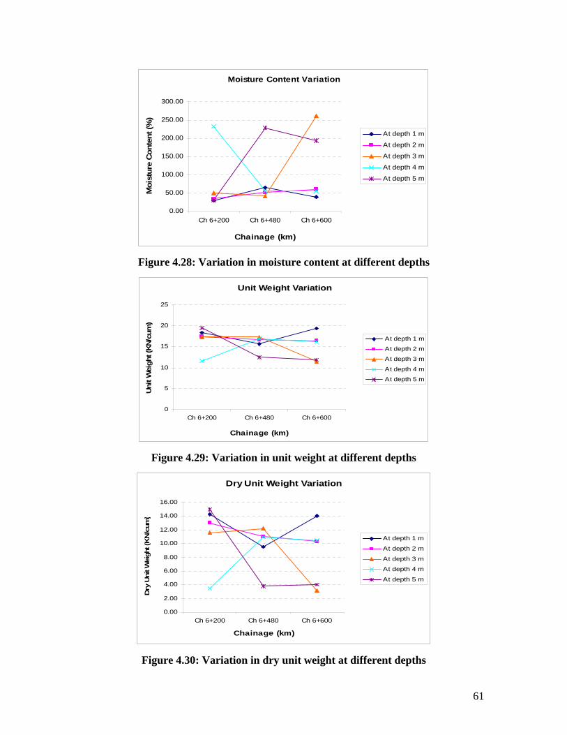
Moisture Content Variation
0.00
50.00
100.00
150.00
200.00
250.00
300.00
Ch 6+200 Ch 6+480 Ch 6+600
Chainage (km)
Moi
stur
e Co
nten
t (%
)
At depth 1 m
At depth 2 m
At depth 3 m
At depth 4 m
At depth 5 m
Figure 4.28: Variation in moisture content at different depths
Unit Weight Variation
0
5
10
15
20
25
Ch 6+200 Ch 6+480 Ch 6+600
Chainage (km)
Unit
Wei
ght (
KN/c
um)
At depth 1 m
At depth 2 m
At depth 3 m
At depth 4 m
At depth 5 m
Figure 4.29: Variation in unit weight at different depths
Dry Unit Weight Variation
0.00
2.00
4.00
6.00
8.00
10.00
12.00
14.00
16.00
Ch 6+200 Ch 6+480 Ch 6+600
Chainage (km)
Dry
Uni
t Wei
ght (
KN
/cum
)
At depth 1 m
At depth 2 m
At depth 3 m
At depth 4 m
At depth 5 m
Figure 4.30: Variation in dry unit weight at different depths
61
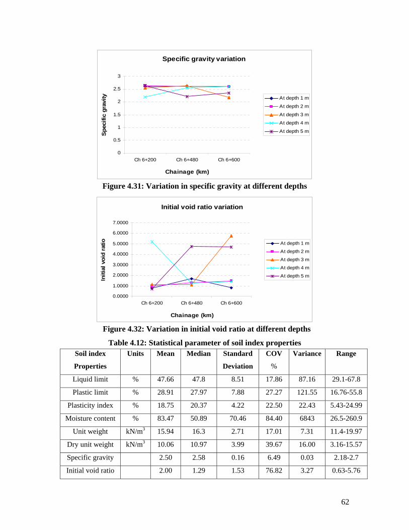
Specific gravity variation
0
0.5
1
1.5
2
2.5
3
Ch 6+200 Ch 6+480 Ch 6+600
Chainage (km)
Spec
ific
grav
ity At depth 1 m
At depth 2 m
At depth 3 m
At depth 4 m
At depth 5 m
Figure 4.31: Variation in specific gravity at different depths
Initial void ratio variation
0.0000
1.0000
2.0000
3.0000
4.0000
5.0000
6.0000
7.0000
Ch 6+200 Ch 6+480 Ch 6+600
Chainage (km)
Initi
al v
oid
ratio At depth 1 m
At depth 2 m
At depth 3 m
At depth 4 m
At depth 5 m
F s
Table 4.12: Statistical parameter of soil index properties
Soil index
Properties
Units Mean Median Standard
Deviation
COV
%
Variance Range
igure 4.32: Variation in initial void ratio at different depth
Liquid limit % 47.66 47.8 8.51 17.86 87.16 29.1-67.8
Plastic limit % 28.91 27.97 7.88 27.27 121.55 16.76-55.8
Plasticity index % 18.75 20.37 4.22 22.50 22.43 5.43-24.99
Moisture content % 83.47 50.89 70.46 84.40 6843 26.5-260.9
Unit weight kN/m3 15.94 16.3 2.71 17.01 7.31 11.4-19.97
Dry unit weight kN/m3 10.06 10.97 3.99 39.67 16.00 3.16-15.57
Specific gravity 2.50 2.58 0.16 6.49 0.03 2.18-2.7
Initial void 0.63-5.76 ratio 2.00 1.29 1.53 76.82 3.27
62
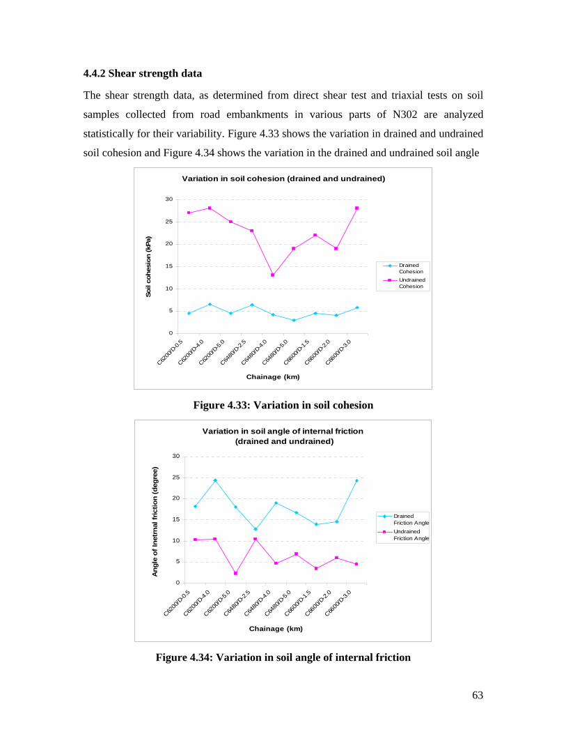
4.4.2 Shear strength data
The shear strength data, as determined from direct shear test and triaxial tests on soil
samples collected from road embankments in various parts of N302 are analyzed
statistically for their variability. Figure 4.33 shows the variation in drained and undrained
soil cohesion and Figure 4.34 shows the variation in the drained and undrained soil angle
Variation in soil cohesion (drained and undrained)
0
5
10
15
20
25
30
C6200
/D-0
.5
C6200
/D-4
.0
C6200
/D-5
.0
C6480
/D-2
.5
C6480
/D-4
.0
C6480
/D-5
.0
C6600
/D-1
.5
C6600
/D-2
.0
C6600
/D-3
.0
Chainage (km)
Soil
cohe
sion
(kPa
)
DrainedCohesionUndrainedCohesion
Figure 4.33: Variation in soil cohesion
Variation in soil angle of internal friction (drained and undrained)
0
5
10
15
20
30
25gree
)
C6200
6200
/48
0/D-4
/D-1
.5
C6600
//D-0
.5/D
-4.0
C6200
C
D-5.0
80/D
-2.5
C64 C6
.0
/D-5
.0
C6480
C6600
D-2.0
00/D
-3
C66
.0
Cha km)
on (d
e
inage (
Ang
le o
f Ine
trna
l fric
ti
Drained rictionF Angle
Undrairictio
nedF n Angle
Figure .34: V tion l angle of internal friction 4 aria in soi
63
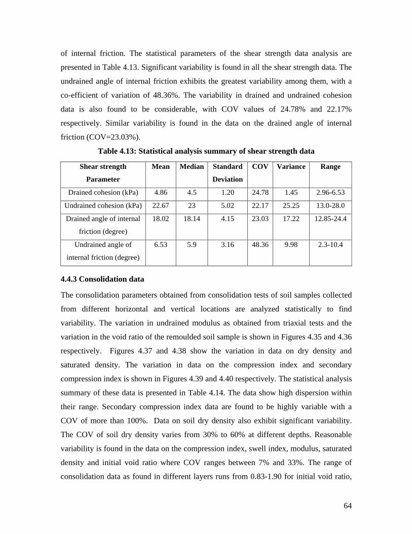
of internal friction. The statistical parameters of the shear strength data analysis are
respectively. Similar variability is found in the data on the drained angle of internal
friction (COV=23.03%).
Table 4.13: Statistical analysis summary of shear strength data
Shear strength
Parameter
Mean Median Standard
Deviation
COV Variance Range
presented in Table 4.13. Significant variability is found in all the shear strength data. The
undrained angle of internal friction exhibits the greatest variability among them, with a
co-efficient of variation of 48.36%. The variability in drained and undrained cohesion
data is also found to be considerable, with COV values of 24.78% and 22.17%
Drained cohesion (kPa) 4.86 4.5 1.20 24.78 1.45 2.96-6.53
Undrained cohesion (kPa) 22.67 23 5.02 22.17 25.25 13.0-28.0
Drained angle of internal
friction (degree)
18.02 18.14 4.15 23.03 17.22 12.85-24.4
Undrained angle of
internal friction (degree)
6.53 5.9 3.16 48.36 9.98 2.3-10.4
4.4.3 Consolidation data
The consolidation param f soil samples collected
from different horizontal and vertical locations are analyzed statistically to find
variability. The variation in undrained modulus as obtained from triaxial tests and the
variation in the void ratio of the remoulded soil sample is shown in Figures 4.35 and 4.36
respectively. Figures 4.37 and 4.38 show the variation in data on dry density and
saturated density. The variation in data on the compression index and secondary
compression index is shown in Figures 4.39 and 4.40 respectively. The statistical analysis
summary of these data is presented in Table 4.14. The data show high dispersion within
their range. Secondary compression index data are found to be highly variable with a
COV of more than 100%. Data on soil dry density also exhibit significant variability.
The COV of soil dry density varies from 30% to 60% at different depths. Reasonable
variability is found in the data on the compression index, swell index, modulus, saturated
density and initial void ratio where COV ranges between 7% and 33%. The range of
consolidation da itial void ratio,
eters obtained from consolidation tests o
ta as found in different layers runs from 0.83-1.90 for in
64
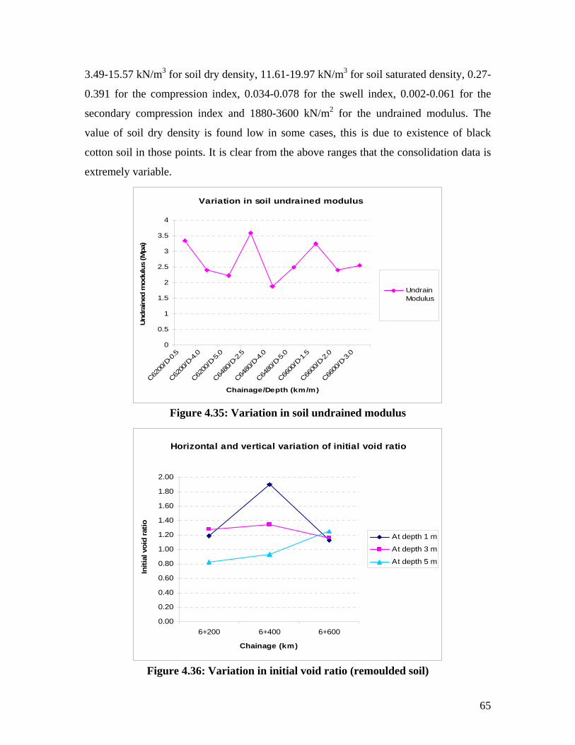
3.49-15.57 kN/m3 for soil dry density, 11.61-19.97 kN/m3 for soil saturated density, 0.27-
0.391 for the compression index, 0.034-0.078 for the swell index, 0.002-0.061 for the
secondary compression index and 1880-3600 kN/m2 for the undrained modulus. The
value of soil dry density is found low in some cases, this is due to existence of black
cotton soil in those points. It is clear from the above ranges that the consolidation data is
extremely variable.
Variation in soil undrained modulus
4
0
D-0.5
D-4.0
0.5
1
1.5
Und
rain
e
2
d m
od
2.5
ulus
(
3
3.5
Mpa
)
Undrainlus Modu
C6200
/
C6200
/
C6200
/D-5
.0
C6480
/D-2
.5
C6480
/D-4
.0
C6480
/D-5
.0
C6600
/D-1
.5
C6600
/D-2
.0
C6600
/D-3
.0
Chainage/Depth (km/m)
Figure 4.35: Variation in soil undrained modulus
Horizontal and vertical variation of initial void ratio
0.00
0.20
0.40
0.60
0.80
1.00
1.20
1.40
1.60
1.80
2.00
6+200 6+400 6+600
Chainage (km)
Initi
al v
oid
ratio
At depth 1 m
At depth 3 m
At depth 5 m
Figure 4.36: Variation in initial void ratio (remoulded soil)
65
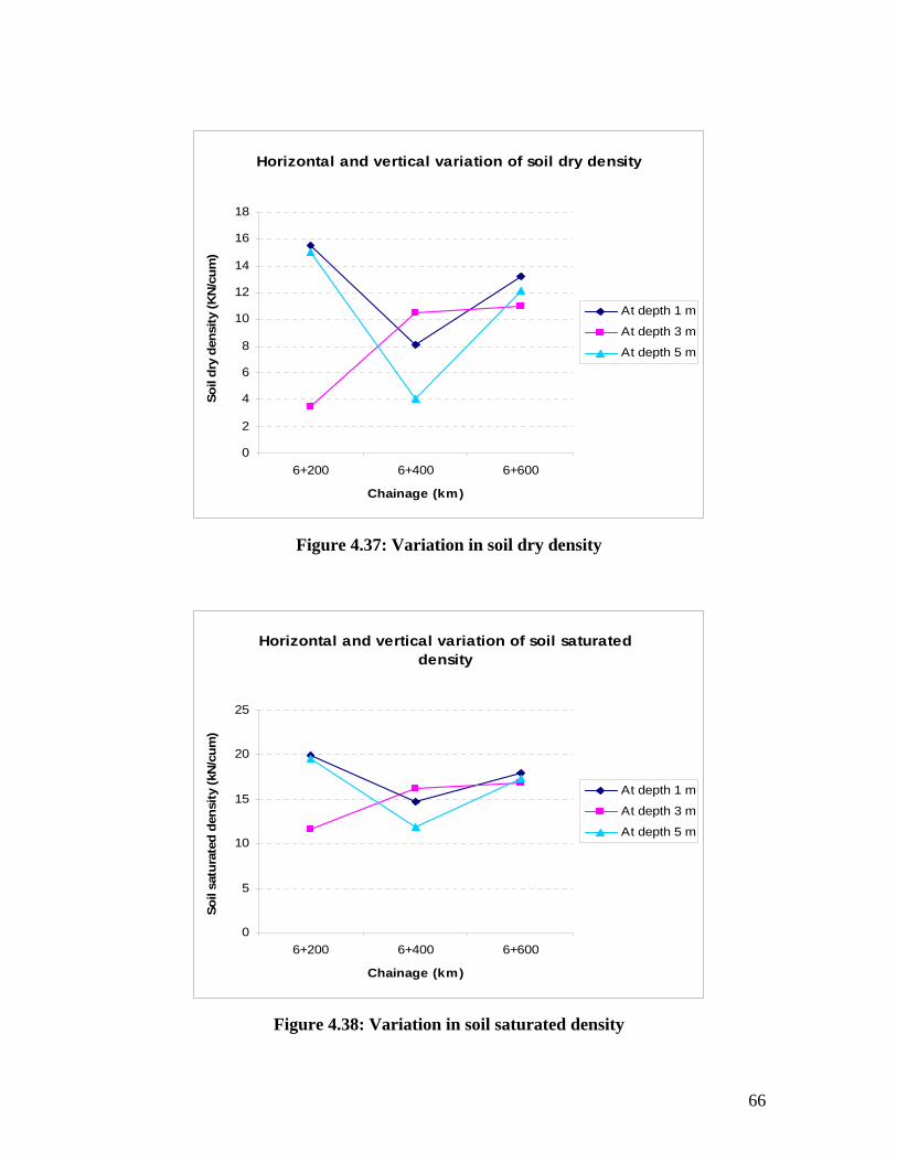
Horizontal and vertical variation of soil dry density
14
16
18cu
m)
0
2
4
6
8
10
12
6+200 6+400 6+600
Chainage (km)
Soil
dry
dens
ity (K
N/
At depth 1 m
At depth 3 m
At depth 5 m
Figure 4.37: Variation in soil dry density
Horizontal and vertical variation of soil saturated density
0
5
10
15
20
25
6+200 6+400 6+600
Chainage (km)
Soil
satu
rate
d de
nsity
(kN
/cum
)
At depth 1 m
At depth 3 m
At depth 5 m
Figure 4.38: Variation in soil saturated density
66
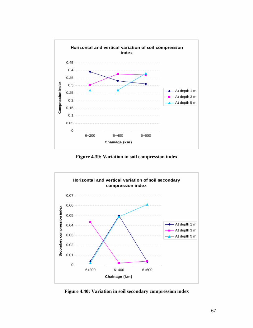
Horizontal and vertical variation of soil compression index
0
0.05
0.1
0.15
0.2
0.25
0.3
0.35
0.4
0.45
6+200 6+400 6+600
Chainage (km)
Com
pres
sion
inde
x
At depth 1 m
At depth 3 m
At depth 5 m
Fig ex ure 4.39: Variation in soil compression ind
Horizontal and vertical variation of soil secondary compression index
0
0.01
0.02
0.03
0.04
0.05
0.06
0.07
6+200 6+400 6+600
Chainage (km)
Seco
ndar
y co
mpr
essi
on in
dex
At depth 1 m
At depth 3 m
At depth 5 m
Figur ndex e 4.40: Variation in soil secondary compression i
67
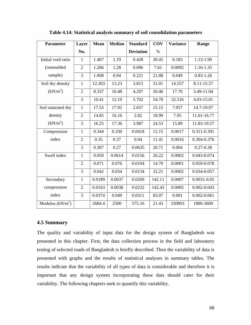
Table 4.14: Statistical analysis summary of soil consolidation parameters
Parameter Layer
No.
Mean Median Standard
Deviation
COV
%
Variance Range
1 1.407 1.19 0.428 30.45 0.183 1.13-1.90
2 1.266 1.28 0.096 7.61 0.0092 1.16-1.35
Initial void ratio
(remoulded
sample) 3 1.008 0.94 0.221 21.88 0.049 0.83-1.26
1 12.303 13.23 3.815 31.01 14.557 8.11-15.57
2 8.337 10.48 4.207 50.46 17.70 3.49-11.04
Soil dry density
(kN/m3)
3 10.41 12.19 5.702 54.78 32.516 4.03-15.01
1 17.53 17.92 2.657 15.15 7.057 14.7-19.97
2 14.85 16.16 2.82 18.99 7.95 11.61-16.77
Soil saturated dry
density
(kN/m3) 3 16.25 17.36 3.987 24.53 15.89 11.83-19.57
1 0.344 0.330 0.0418 12.15 0.0017 0.311-0.391
2 0.35 0.37 0.04 11.41 0.0016 0.304-0.376
Compression
index
3 0.307 0.27 0.0635 20.71 0.004 0.27-0.38
1 0.059 0.0614 0.0156 26.22 0.0002 0.043-0.074
2 0.071 0.076 0.0104 14.70 0.0001 0.059-0.078
Swell index
3 0.042 0.034 0.0134 32.21 0.0002 0.034-0.057
1 0.0189 0.0037 0.0269 142.11 0.0007 0.0031-0.05
2 0.0163 0.0038 0.0232 142.43 0.0005 0.002-0.043
Secondary
compression
index 3 0.0374 0.049 0.0311 83.07 0.001 0.002-0.061
Modulus (kN/m2) 2684.4 2500 575.16 21.43 330803 1880-3600
4.5 Summary
The quality and variability of input data for the design system of Bangladesh was
presented in this chapter. First, the data collection process in the field and laboratory
testing of selected roads of Bangladesh is briefly described. Then the variability of data is
presented with graphs and the results of statistical analyses in summary tables. The
results indicate that the variability of all types of data is considerable and therefore it is
important that any design system incorporating these data should cater for their
variability. The following chapters seek to quantify this variability.
68
Chapter 5 Pavement Design Risk and Reliability
5.1 Introduction
This chapter describes the com ent process of the m
the pavem The available m
quantifying pavement design ri are assessed with regard to their suitability and
appli n the de n s esh. Then the logical development leading
to the design of a s able od ang is ted lly
description of the proposed is ed.
5.2 Assessment of th methods
A k and liab eth ave ee lop ass
these f .
Austroads [2004]: e A ds 4] c red diffe
labo onditi s an rv diti el d in
predicted service lif due ari in ct vi t and traffic.
However, the in-service conditions in Bangla e di fro
Aus e the nvi t ngl s totally different. The traffic
cha nd th har c pa co ion gla
signifi those in Australia. Hence, th ent lop Aus
section 2.7.1) seem no o b b he d yst a .
AASHTO [1993]: The risk analysis technique of this guide is simple, but considers an
mance prediction model to estimate the variance in pavement
sh.
plete developm ethod of quantifying
ent design risk for Bangladesh. ethods for the process of
sk
cability i sig ystem of Banglad
uit meth for B ladesh presen . Fina a detailed
method provid
e available
number of ris
ollows
re ility m ods h so far b n deve ed. An essment of
Th ustroa [200 method onside the rences in
ratory test c on d in-se ice con ons as w l as the ifference actual and
e to v ability constru ion, en ronmen
desh ar totally fferent m those in
tralia, sinc
racteristics a
cantly from
e ronmen of Ba adesh i
e c acteristi s of the vement nstruct in Ban desh differ
e elem s deve ed by troads (see
t t e applica le for t esign s em of B ngladesh
empirical perfor
performance. The proposed design method for Bangladesh is analytical and considers
only those design data which apply to analytical pavement design. Consequently, this
method is not entirely suitable for the design system of Bangladesh.
The methods of both Noureldin et al. [1994, 1996] and Huang [1993] are variants of the
AASHTO method.
NCHRP [2004]: The method proposed in this M-E design guide incorporates long term
pavement distress data which are not currently available in Banglade
69
Kim [20 model.
ent failure due to rutting is not predominant in Bangladesh.
method did not consider the risk associated with the variability in the
factors affecting pavement design. Hence, the method is not suitable for developing a
ethod uses the present serviceability index
mulation. But the design system of Bangladesh requires a tool which is
imple and suitable for analytical pavement design system. A
rocedure did not
completely fulfil the task in hand.
06]: The technique proposed in this method considers a rut prediction
However, pavem
TRRL [1975]: The
system which could analyse the variability in the pavement design data and associated
risk.
Chua et al. [1992]: The proposed method is also not suitable for the design system of
Bangladesh, since it involves computational difficulties to perform multi-fold integration
for a high number of variables. The method requires a computer program to perform the
analysis.
Alsherri and George [1988]: The suggested m
to formulate a reliability model using the AASHTO [1972, 1986] design model and the
Monte Carlo si
simple and suitable for analytical pavement design.
Kulkarni [1994]: The method is based on historical pavement performance data which
are not available in Bangladesh and no arrangement has been made yet for the future
collection of long term pavement performance data. Thus this method is not suitable for
Bangladesh.
Zhang [2006]: The method proposed by Zhang [2006] requires time series data which
are not available in Bangladesh. Hence, the method cannot be applied in the design
system of Bangladesh.
Lua et al. [1996]: This reliability analysis method is based on a finite element pavement
response model. But the pavement design method which is proposed for Bangladesh
considers the method of using the equivalent thickness design model for the structural
analysis of pavement. As a result, this reliability analysis method is not suitable for the
pavement design system of Bangladesh.
Brown [1994]: The uncertainty estimation technique of this method, performing a
sensitivity analysis, is s
safety factor also was suggested to apply in a convenient manner. But the safety factor
determination and application procedure is not well defined. Hence the p
70

The above points are summarised in Table 5.1.
Table 5.1: The summary of the suitability of the available methods
reliability analytical (available data design
onal
re
Available
Methods
Accurately
determine
risk and
Suitable for
use in the
proposed
Suitable for
the conditions
in Bangladesh
Consider all
the variables
in pavement
Easy
Computati
procedu
due to data
variability
pavement
design
system
and failure
mode)
Austroads [2004] Yes Yes No Yes Yes
AASHTO [1993] Yes No No Yes Yes
Noureldin et al.
[1994, 1996]
Yes No No Yes Yes
Huang [1993] Yes No No Yes Yes
NCHRP [2004] Yes Yes No Yes Yes
Kim [2006] Yes Yes No Yes No
TRRL [1975] No No No No Yes
Chua et al. [1992] Yes Yes No Yes No
Alsherri and
George [1988]
Yes No No Yes Yes
Kulkarni [1994] Yes Yes No Yes Yes
Zhang [2006] Yes Yes No Yes No
Lua et al. [1996] Yes No Yes Yes No
Brown [1994] No Yes Yes Yes Yes
71
5.3 Proposed Approach
5.3.1 Development of the proposed method
Comp ria as
methodology chapter shows that no m
design system of Bangladesh. Therefore this research develops a
pavement design data variabil ining re or such tem. The
reliability determination ure of AASHTO
[1993], but a different approach is developed to com ent
performance since the empirical p performance equation which is used to
construct the variance of pavement performance in AASHTO’s me
s al p ent design. The analytical pavement design system be
p glades dicts pav nt perform using a p ent structu
a l based on layered elastic theory in association with the method of
equivalent thickness. Thus, this research develops a procedure to dete e the varia
o icting ent per nce, due to the variability in the design d
The theory of the first order approxim approach sed in this To determ
t traffic prediction, this research uses the first or approximat
a s als d by No in et al. [1996] and Huang [1993]. Then
overall variance and reliability design factor are calcu using the ions propo
by AASHTO [1993] as discussed in section 2.7.2. A detailed description of this proposed
m ed in n 5.3.2. proposed m od is suita r designin
p e desired ree of reliability. However, it is some necessary
d bility existing pavement. To nd an alter e procedure
proposed in this research. In the alternative approach, the safety factor of the pavem
ructure is determined first as a ratio of pavement capacity (predicted performance) and
emand (predicted traffic). The same pavement structural analysis model as discussed
efore is used to evaluate pavement capacity. Then a risk analysis of the safety factor for
ifferent traffic and pavement performance prediction parameters is conducted. The
eory of mean first order second moment method, which was used by many researchers
aring the available methods with respect to the
ity a
concept of this m
crite
be found com
defined in the
pletely suitable for the
method of quantifying
a sys
ethod can
nd determ
ethod is sim
avement
liability f
ilar to the proced
pute the variance in pavem
thod [1993] is not
uitable for analytic avem ing
roposed for Ban
nalysis mode
h pre eme ance avem ral
rmin nce
f this model pred pavem forma ata.
ation is u task. ine
he variance in der ion
pproach which wa o use ureld the
lated equat sed
ethod is present sectio The eth ble fo g a
avement of th deg times to
etermine the relia of an this e nativ is
ent
st
d
b
d
th
72
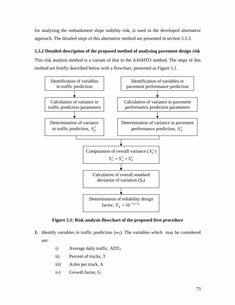
for analysing the embankment slope stability risk, is used in the developed alternative
approach. The detailed steps of this alternative method are presented in section 5.3.3.
iv) Growth factor, G
5.3.2 Detailed description of the proposed method of analysing pavement design risk
This risk analysis method is a variant of that in the AASHTO method. The steps of this
method are briefly described below with a flowchart, presented as Figure 5.1.
Figure 5.1: Risk analysis flowchart of the proposed first procedure 1. Identify variables in traffic prediction (wT). The variables which may be considered
are:
i) Average daily traffic, ADT0
ii) Percent of trucks, T
iii) Axles per truck, A
Identification of variables in traffic prediction
Calculation of variance in traffic prediction parameters
Identification of variables in pavement performance prediction
Calculation of variance in pavement performance prediction parameters
Computation of overall variance ( 20S )
2220 Nw SSS +=
Determination of variance in traffic prediction, 2
wS Determination of variance in pavement
performance prediction, 2NS
Calculation of overall standard deviation of variation (S0)
Determination of reliability design factor, 010 SZ
RRF ×−=
73
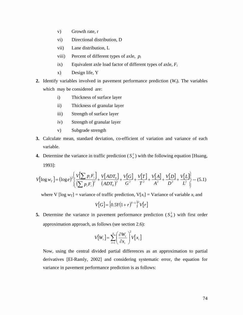
v) Growth rate, r
vi) Directional distribution, D
vii) Lane distribution, L
i
2. Iden ent perfor ariables
which e:
i) Thickness of surface layer
ular layer
layer
iv) Strength of granular layer
n h
3. Calculate mean, standard deviation, co-efficient of variation and variance of each
variable.
4. Determine the variance fol wing equation [Huang,
1993]:
viii) Percent of different types of axle, p
ix) Equivalent axle load factor of different types of axle, Fi
x) Design life, Y
mance prediction (Wt). The vtify variables involved in pavem
may be considered ar
ii) Thickness of gran
iii) Strength of surface
v) Subgrade stre gt
in traffic prediction ( 2wS ) with the lo
[ ] ( ) [ ]( )
[ ]( )
[ ] [ ] [ ] [ ] [ ]⎪⎭
⎪⎬⎫
⎪⎩
⎪⎨⎧
++=∑∑
22222loglog
LLV
DDVAADTV
Fp
FpVewV
ii
iiT -- (5.1)
where V [log wT] = variance of traffic prediction, V[xi] = Variance of variable xi and
++++ 2220
0
AV
TTV
GGV
ADT
[ ] ( ){ } [ ]rVrYGV Y 2115.0 −+=
ment p5. Determine the variance in pave erformance prediction ( ) with first order
appro
2NS
ximation approach, as follows (see section 2.6):
[ ] [ ]ii i
tt xV
xWV
1∑=
⎟⎟⎠
⎜⎜⎝ ∂
=
Now,
n W2⎞⎛ ∂
using the central divided partial differences as an approximation to partial
ring systematic error, the equation for
rediction is as follows:
derivatives [EI-Ramly, 2002] and conside
variance in pavement performance p
74

n
[ ] [ ]systematici
n
i i
ti[ ]
i i
t xVxWW
2
1
2
∑=
⎟⎟⎠
⎞⎜⎜⎝
⎛ΔΔ
+⎞⎛ Δ
------------- (5.2)
ance prediction.
rediction parameters xi
hich could be
d as V[xi]/n [Freund, 1979] where n = sample size.
ed to evaluate the changes in pavement performance
i). A structural analysis model based on the
ed in the present research for this purpose.
6. llows [AASHTO, 1993]:
Overall V rediction ( + Variance in Pavement
the overall standard deviation of variation ( as follows:
e the reliability design factor for a desired reliability level as follows
[AASHTO, 1993]:
--------------------------------------- (5.4)
x
E-4] for a given reliability level, R.
9. Incorporate reliability in design by multiplying the predicted traffic with the reliability
5.3.3 Proposed alternative approach of analysing pavement design risk (FOSM)
ernative method is presented in Figure 5.2 and the detailed
1.
ion 5.3.2.
2. Calculate the mean, standard deviation, co-efficient of variation and variance of each
variable. Also calculate the variance of mean due to systematic error (see sec. 5.3.2).
t xVx
WV1∑=
⎟⎟⎠
⎜⎜⎝ Δ
=
where V [Wt] = Variance in pavement perform
V[xi] = Variance of pavement performance p
V[xi]systematic = Variance of variables xi due to systematic error w
estimate
Δ Wt = Change in pavement performance due to change of variable xi
A sensitivity analysis is perform
(Δ Wt) due to changes in each variable (Δx
method of equivalent thickness (MET) is us
Calculate the overall variance ( 2S ) as fo0
2 2wS )ariance ( 0S ) = Variance in Traffic P
Performance Prediction ( 2NS ) …………..……………….. (5.3)
7. Determine 0S )
Overall Standard Deviation of Variation ( 0S ) = √ Overall Variance
8. Calculat
010 SZR
RF ×−=
where the value ZR can be found from standard normal curve area tables [Appendi
design factor to estimate the design traffic
A flowchart of the proposed alt
steps of this method are described below:
Identify variables in traffic prediction (wT) and pavement performance prediction (Wt).
The variables which may be considered are described in sect
75
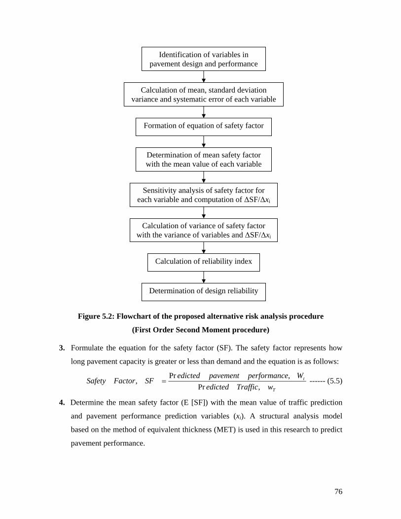
Identification of variables in pavement design and performance
Calculation of mean, standard deviation variance and systematic error of each variable
Formation of equation of safety factor
Determination of mean safety factor with the mean value of each variable
Sensitivi analysis of safety factor for ty each variable and computation of ΔSF/Δxi
Calculation of variance of safety factor with the variance of variables and Δxi
ond Moment procedure)
n demand and the equation is as follows:
Figure 5.2: Flowchart of the proposed alternative risk analysis procedure
(First Order Sec
3. Formulate the equation for the safety factor (SF). The safety factor represents how
long pavement capacity is greater or less tha
T
4. Determine the mean safety factor (E [SF]
tWeperformancpavementedictedSFFactorSafety
,Pr, = ------ (
wTrafficedicted ,Pr5.5)
) with the mean value of traffic prediction
and pavement performance prediction variables (xi). A structural analysis model
based on the method of equivalent thickness (MET) is used in this research to predict
pavement performance.
ΔSF/
Calculation of reliabilit index y
Determination of design reliability
76
5. Perform a sensitivity analys e safety factor (ΔSF) due to
changes in each variable
6. Determine the variance of the safety factor (V [SF]) with the first order approximation
approach (see section
is to evaluate the changes in th
(Δ xi).
2.6) as follows:
[ ]i
n
i ix1= ⎠⎝ ∂xVSFSFV ][ ∑ ⎟⎟
⎞⎜⎜⎛ ∂
=
Now, using divided differences as an approximation to partial derivative [EI-Ramly,
2002] and considering ariance of safety factor
takes the following form
2
systematic error, the equation for v
:
[ ] [ ] errorsystematicii i
spatialii i
xVx
xVx 11
∑∑==
⎟⎟⎠
⎜⎜⎝ Δ
+⎟⎟⎠
⎜⎜⎝ Δ
nn SFSFSFV22
][⎞⎛ Δ⎞⎛ Δ
= -------- (5.6)
where V[xi]spatial = Variance of traffic and performance prediction variables xi
V[xi]systematic = c error.
7. Calculate the standar s:
Variance of variables xi due to systemati
d deviation of safety factor (σ [SF]) as follow
][,][ SFVfactorsafetyofVarianceSF =σ
8. Calculate the reliability i e value of 1 at limit state.
Hence, the equation for reliability index could be written as;
ndex. The safety factor takes th
[ ][ ]SF
SFE 0.1σ
β −= ---------------------------------------- (5.7)
9. D
the corresponding v
5.4 Su
The chapter presented the complete development process of the proposed method of
analyzing the pavement design risk for Bangladesh. First, a comparison of
met
the
Fin ethods were presented in detail.
etermine the reliability of pavement from the standard normal curve area Table for
alue of the reliability index (Appendix E-1).
mmary
the existing
method of analyzing pavement design risk with respect to the criteria as defined in the
hodology chapter was briefly presented. Then the theory and concept used to develop
proposed risk analysis method for the pavement design of Bangladesh was discussed.
ally the procedures of two alternative proposed m
77
Chapter 6 Embankment Design Risk and Reliability
A prime objective of this research project as described in Chapter 1 was to quantify the
risk in embankment design due to the variability in data. To this end, the literature review
chapter reviewed the embankment design procedures and design data, variability in
des
the
the light of slope stability and settlement so as to incorporate the findings in the design
system of Bangladesh. Accordingly, the chapter first briefly compares the e
stability risk analysis methods considering the criteria as mentioned in methodology
cha tly, the
sug of this chapter
settlement risk.
re which is proposed in this research for analyzing the embankment
6.2 Embankment slope st
6.2.1 Assessment of the available methods
emb
nd moment method: the first order second moment method requires
fewer calculations and less computing time than other methods do. This method is widely
powerful and offers a practical tool for more detailed analysis of slope stability when
6.1 Introduction
ign data, variability quantification and risk analysis methods. This chapter considers
development of a suitable procedure for quantifying the embankment design risk in
xisting slope
pter to judge their suitability for the design system of Bangladesh. Subsequen
gested method for Bangladesh is presented in detail. The later part
presents a similar comparison of the methods developed for analyzing
Finally, the procedu
settlement risk in Bangladesh is discussed in detail.
ability risk analysis
A number of methods have been developed for analysing the stability risk of
ankment slopes. An assessment of these follows.
First order seco
used and well recognized. It is easy to implement and requires no computer program. It
can consider the variability of all slope stability design parameters and can be applied
using the data available in Bangladesh.
Point estimation method: the point estimation method is complex and hence not popular
in practice.
Monte Carlo simulation method: the Monte Carlo simulation method has been proved
78
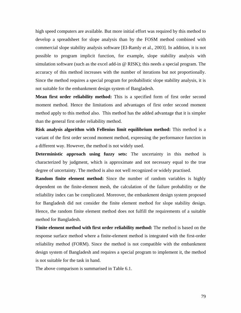
high s od to
than by the FOSM method combined with
ability analysis software [EI-Ramly et al., 2003]. In addition, it is not
possible to program implicit function, for example, slope stability analysis with
t necessary equal to the true
cognized or widely practised.
Random finite element method: Since the number of random variables is highly
alculation of the failure probability or the
method for slope stability design.
method is not compatible with the embankment
for the task in hand.
peed computers are available. But more initial effort was required by this meth
develop a spreadsheet for slope analysis
commercial slope st
simulation software (such as the excel add-in @ RISK); this needs a special program. The
accuracy of this method increases with the number of iterations but not proportionally.
Since the method requires a special program for probabilistic slope stability analysis, it is
not suitable for the embankment design system of Bangladesh.
Mean first order reliability method: This is a specified form of first order second
moment method. Hence the limitations and advantages of first order second moment
method apply to this method also. This method has the added advantage that it is simpler
than the general first order reliability method.
Risk analysis algorithm with Fellenius limit equilibrium method: This method is a
variant of the first order second moment method, expressing the performance function in
a different way. However, the method is not widely used.
Deterministic approach using fuzzy sets: The uncertainty in this method is
characterized by judgment, which is approximate and no
degree of uncertainty. The method is also not well re
dependent on the finite-element mesh, the c
reliability index can be complicated. Moreover, the embankment design system proposed
for Bangladesh did not consider the finite element
Hence, the random finite element method does not fulfill the requirements of a suitable
method for Bangladesh.
Finite element method with first order reliability method: The method is based on the
response surface method where a finite-element method is integrated with the first-order
reliability method (FORM). Since the
design system of Bangladesh and requires a special program to implement it, the method
is not suitable
The above comparison is summarised in Table 6.1.
79
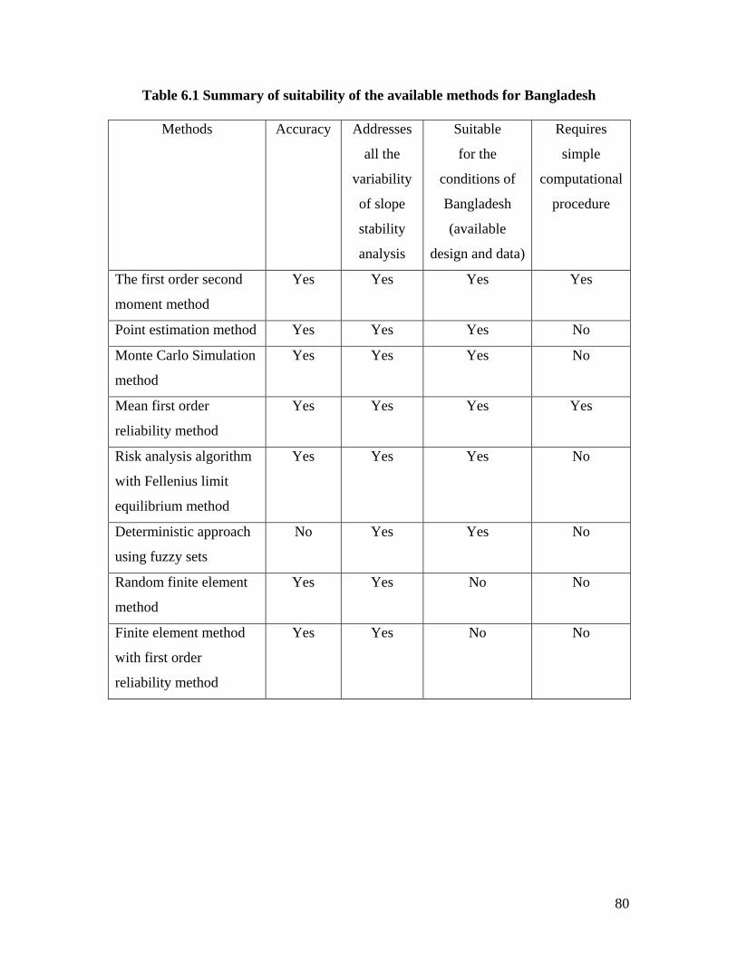
Table 6.1 Summary of suitability of the available methods for Bangladesh
Methods Accuracy Addresses
all the
variability
of slope
stability
analysis
Suitable
for the
conditions of
Bangladesh
(available
design and data)
Requires
simple
computational
procedure
The first order second Yes Yes Ye
moment method
s Yes
Point estimation method Yes Yes Yes No
Monte Carlo Simulation
method
Yes Yes Yes No
Mean first order
reliability method
Yes Yes Yes Yes
Risk analysis algorithm Yes Yes Yes No
with Fellenius limit
equilibrium method
Deterministic approach
using fuzzy sets
No Yes Yes No
Random finite element
method
Yes Yes No No
Finite element method
with first order
Yes Yes No No
reliability method
80
6.2.2
From the on shown .1 that sec nt
method is widely used, easily implemen requires puter program and
performs its function reasonably accurate on, n
with the data available in Bangladesh. Hen ethod ded n
system of Bangladesh.
To perform risk analysis with the first on d, a method of
analysing slope stability is required. Analysis methods of tw ds, simplifie thods
a methods, are commonly used to analyze slope stability. Although the
f bee reasingl d in recen rs [Griffiths lane,
1 ffiths Fenton, , the simplified methods which rely on
s g the assumptions on the location of the slip surface, rigid body displacements,
s . have been ely prac and are w recognized for slope
stability analysis [Tang et al., 1976, Christian, 1994; EI-Ramly, 2002; Venmarcke, 1977;
L bosa , 1989]. ral simplified methods are available in
t ased on different assumptions. Among them, Spencer’s method
[ re accurate but rigorous. The simplified Bishop method [Bishop,
1 widely d althou atisfies on overall moment and is
applicable to a circular slip surface. The investigation carried out by Malkawi et al.
[ iscrep s betwe results of other methods and those of
the Spencer method range from 0.04 to 0.1. Since the Bishop method is simple, well
r ciated s which ot too larg e present rese uses
t robabilistic risk assessment.
The steps of the suggested risk analysis method are briefly described below and a
Identify the variables which affect the stability of the embankment slope. The
variables which may be considered are:
i) Cohesion, c´
ii) Angle of internal friction, Ф´
iii) Unit weight, γ
Suggested Approach
comparis in Table 6 , it appears
table,
ly. In additi
ce this m
order sec
the first order
no com
the method ca
is recommen
ond mome
be implemented
for the desig
d moment metho
o kin d me
nd finite element
inite element method has n inc y use t yea and
999; Zou et al. 1995; Gri
implifyin
and 2004]
oil properties etc wid tised idely
i and Lumb, 1987; Bara
he literature, each b
Spencer, 1967] is mo
et al. Seve
955] is very simple and use gh it s ly the
2000] showed that the d ancie en the
ecognized and has asso
his method for p
error are n e, th arch
flowchart is presented as Figure 6.1.
1.
81
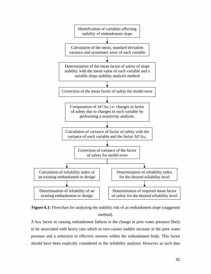
Identification of variables affecting stability of embankment slope
Calculation of the mean, standard deviation variance and systematic error of each variable
Determination of the mean factor of safety of slope stability with the mean value of each variable and a
suitable slope stability analysis method
Computation of ΔF/Δxi i.e. changes in factor of safety due to changes in each variable by
performing a sensitivity analysis.
Calculation of variance of factor of safety with the variance of each variable and the factor ΔF/Δxi.
Calculation of reliability index of an existing embankment or design
od).
A ankment failures is the change in pore water pressure likely
to rn causes sudden increase in the pore water
ithin the embankment body. This factor
should have been explicitly considered in the reliability analysis. However as such data
Correction of variance of the factor of safety for model error
Correction of the mean factor of safety for model error
Determination of reliability index for the desired reliability level
Figure 6.1: Flowchart for analyzing the stability risk of an embankment slope (suggested
meth
key factor in causing emb
be associated with heavy rain which in tu
pressure and a reduction in effective stresses w
Determination of reliability of an existing embankment or design
Determination of required mean factor of safety for the desired reliability level
82
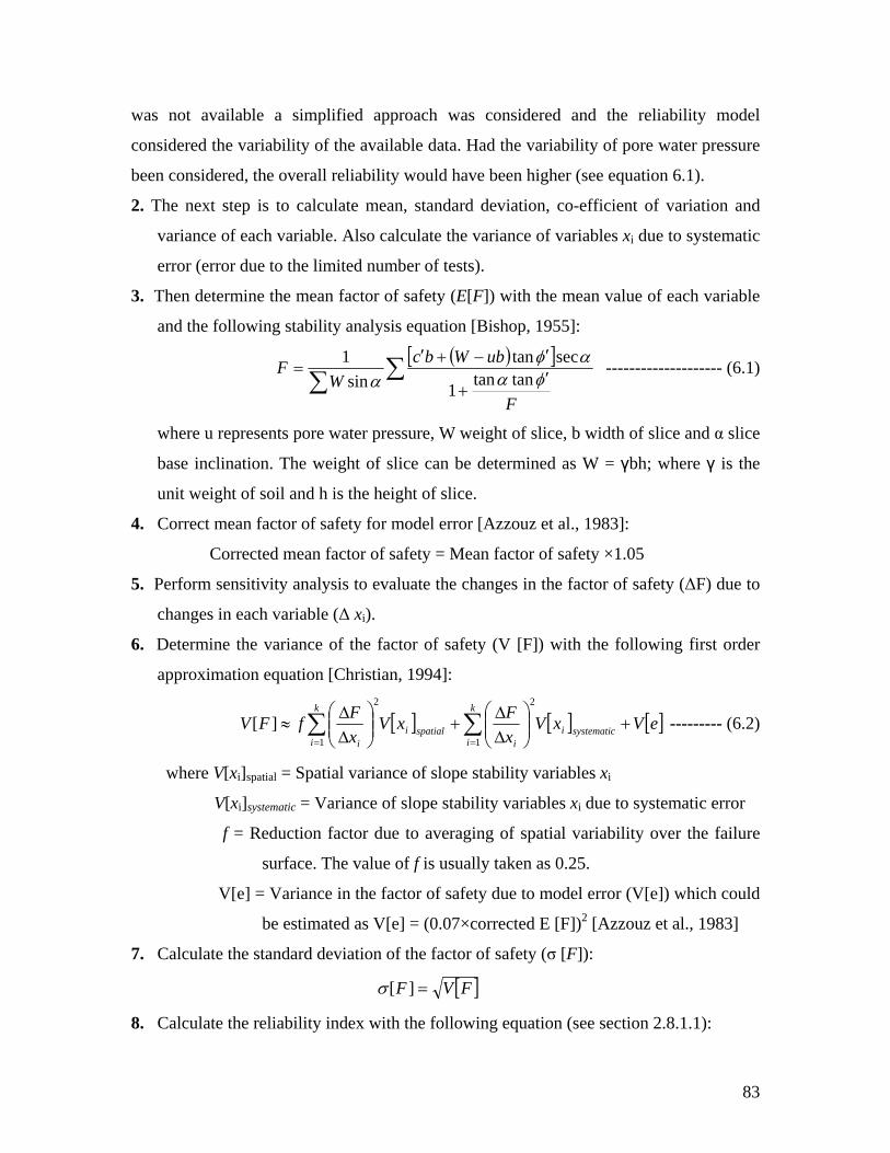
was not available a simp d the reliability model
considered the variability of th of pore water pressure
been considered, the overall reliability would have been higher (see equation 6.1).
2. The next step is to ent of variation and
variance of each variab xi due to systematic
error (error due to the li
3. Then determine of each variable
and the following stab
lified approach was considered an
e available data. Had the variability
calculate mean, standard deviation, co-effici
le. Also calculate the variance of variables
mited number of tests).
the mean factor of safety (E[F]) with the mean value
ility analysis equation [Bishop, 1955]:
( )[ ]∑∑ ′+
′ ′+ −=
F
ubWbcFW φα
φα tantan1sin
αsectan1 -------------------- (6.1)
where u represents pore water pressure, W weight of slice, b width of slice and α slice
base inclination. Th γbh; where γ is the
unit weight of soil and h
4. Correct mean factor of safety for model error [Azzouz et al., 1983]:
Corrected 5
5. Perform sensitivity safety (ΔF) due to
changes in each variable (Δ x ).
6. Determine the variance the following first order
approximation equation [Christian, 1994]:
e weight of slice can be determined as W =
is the height of slice.
mean factor of safety = Mean factor of safety ×1.0
analysis to evaluate the changes in the factor of
i
of the factor of safety (V [F]) with
[xVxFfFV i
i i⎟⎟⎠
⎞⎜⎜⎝
⎛ΔΔ
≈ ∑=1
][ ] [ ] [ ]eVxVxF
systematicii
+⎟⎟⎠
⎞ΔΔ --------- (6
k
ispatial
k
⎜⎜⎝
⎛+∑
=
2
1
2
.2)
where V[xi]spatial = Spatial variance of slope stability variables xi
lope stab
to averag
V[e] = Variance in the factor of safety due to model error (V[e]) which could 2
ility variables xi due to systematic error
ing of spatial variability over the failure
V[xi]systematic = Variance of s
f = Reduction factor due
surface. The value of f is usually taken as 0.25.
be estimated as V[e] = (0.07×corrected E [F]) [Azzouz et al., 1983]
7. Calculate the standard deviation of the factor of safety (σ [F]):
[ ]FVF =][σ
8. Calculate the reliability index with the following equation (see section 2.8.1.1):
83
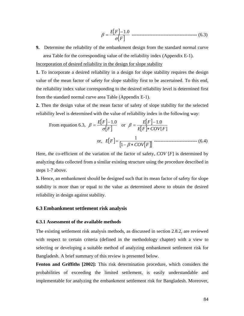
[ ][ ]F
FEσ
β 0.1−= ----------------------------------------- (6.3)
9. Determine the reliability of the embankment design from the standard normal curve
Inc
area Table for the corresponding value of the reliability index (Appendix E-1).
orporation of desired reliability in the design for slope stability
o incorporate a desired reliability in a design f1. T or slope stability requires the design
the level is determined first
from the standard normal curve area Table (Appendix E-1).
2. Then the design value of the mean factor of safety of slope stability for the selected
reliability level is determined with the value of reliability index in the following way:
value of the mean factor of safety for slope stability first to be ascertained. To this end,
reliability index value corresponding to the desired reliability
From equation 6.3, [ ][ ]F
FEσ
β 0.1−= or [ ]
[ ] ][0.1
FCOVFEFE∗
−=β
or, [ ] [ ][ ]FCOVFE
∗−=
β1 -------------1 -------------- (6.4)
determined by
step
stab s determined above to obtain the desired
reliability in design against stability.
6.3 Em
6.3
with respect to c apter) with a view to
Bangladesh. A brie
, which considers the
limited settlement, is easily understandable and
over,
Here, the co-efficient of the variation of the factor of safety, COV [F] is
analyzing data collected from a similar existing structure using the procedure described in
s 1-7 above.
3. Hence, an embankment should be designed such that its mean factor of safety for slope
ility is more than or equal to the value a
bankment settlement risk analysis
.1 Assessment of the available methods
The existing settlement risk analysis methods, as discussed in section 2.8.2, are reviewed
ertain criteria (defined in the methodology ch
selecting or developing a suitable method of analyzing embankment settlement risk for
f summary of this review is presented below.
Fenton and Griffiths [2002]: This risk determination procedure
probabilities of exceeding the
implementable for analyzing the embankment settlement risk for Bangladesh. More
84
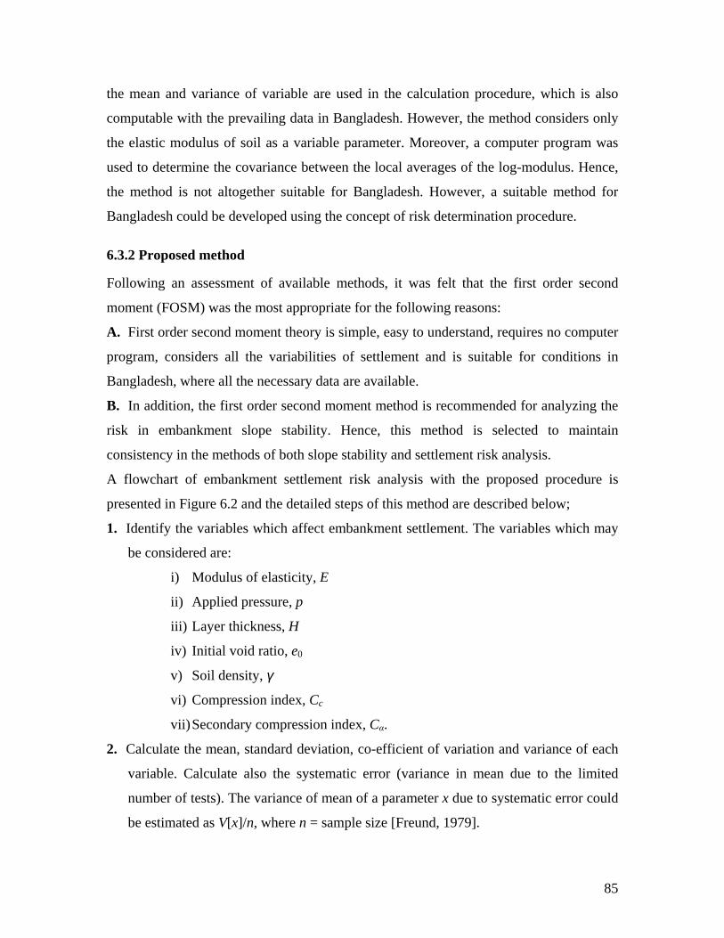
the mean and variance of variabl the calculation procedure, which is also e are used in
computable with the prevailing data in Bangladesh. However, the method considers only
use ence,
a suitable method for
that the first order second
ter
program, considers all the variabilities of settlement and is suitable for conditions in
ary data are available.
oment method is recommended for analyzing the
ence, this method is selec
re 6.2 and the detailed steps of this method are described below;
ii) Applied pressure, p
each
the elastic modulus of soil as a variable parameter. Moreover, a computer program was
d to determine the covariance between the local averages of the log-modulus. H
the method is not altogether suitable for Bangladesh. However,
Bangladesh could be developed using the concept of risk determination procedure.
6.3.2 Proposed method
Following an assessment of available methods, it was felt
moment (FOSM) was the most appropriate for the following reasons:
A. First order second moment theory is simple, easy to understand, requires no compu
Bangladesh, where all the necess
B. In addition, the first order second m
risk in embankment slope stability. H ted to maintain
consistency in the methods of both slope stability and settlement risk analysis.
A flowchart of embankment settlement risk analysis with the proposed procedure is
presented in Figu
1. Identify the variables which affect embankment settlement. The variables which may
be considered are:
i) Modulus of elasticity, E
iii) Layer thickness, H
iv) Initial void ratio, e0
v) Soil density, γ
vi) Compression index, Cc
vii) Secondary compression index, Cα.
2. Calculate the mean, standard deviation, co-efficient of variation and variance of
variable. Calculate also the systematic error (variance in mean due to the limited
number of tests). The variance of mean of a parameter x due to systematic error could
be estimated as V[x]/n, where n = sample size [Freund, 1979].
85
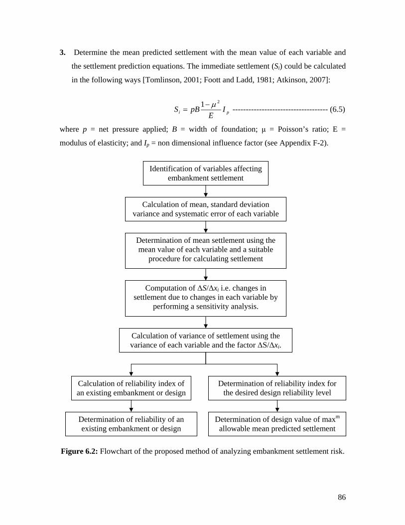
3. Determine the mean predicted settlement with the mean value of each variable and
the settlement prediction equations. The immediate settlement (Si) could be calculated
in the following ways [Tomlinson, 2001; Foott and Ladd, 1981; Atkinson, 2007]:
pi IE
pBS21 μ−
= ------------------------------------ (6.5)
where p = net pressure applied; B = width of foundation; μ = Poisson’s ratio; E =
Ip = non dimensional influence factor (see Appendix F-2).
Fig
modulus of elasticity; and
Identification of variables affecting embankment settlement
Calculation of mean, standard deviation variance and systematic error of ea
ure 6.2: Flowchart of the proposed method of analyzing embankment settlement risk.
ch variable
Determination of mean settlement using the mean value of each variable and a suitable
procedure for calculating settlement
Computation of ΔS/Δx i.e. changes in isettlement due to changes in each variable by
performing a sensitivity analysis.
Calculation of variance of settlement using the ach variable and the factor ΔS/Δxi. variance of e
Calculation of reliability index of an existing embankment or design
Determination of reliability index for the desired design reliability level
Determination of reliability of an existing embankment or design
Determination of design value of maxm allowable mean predicted settlement
86
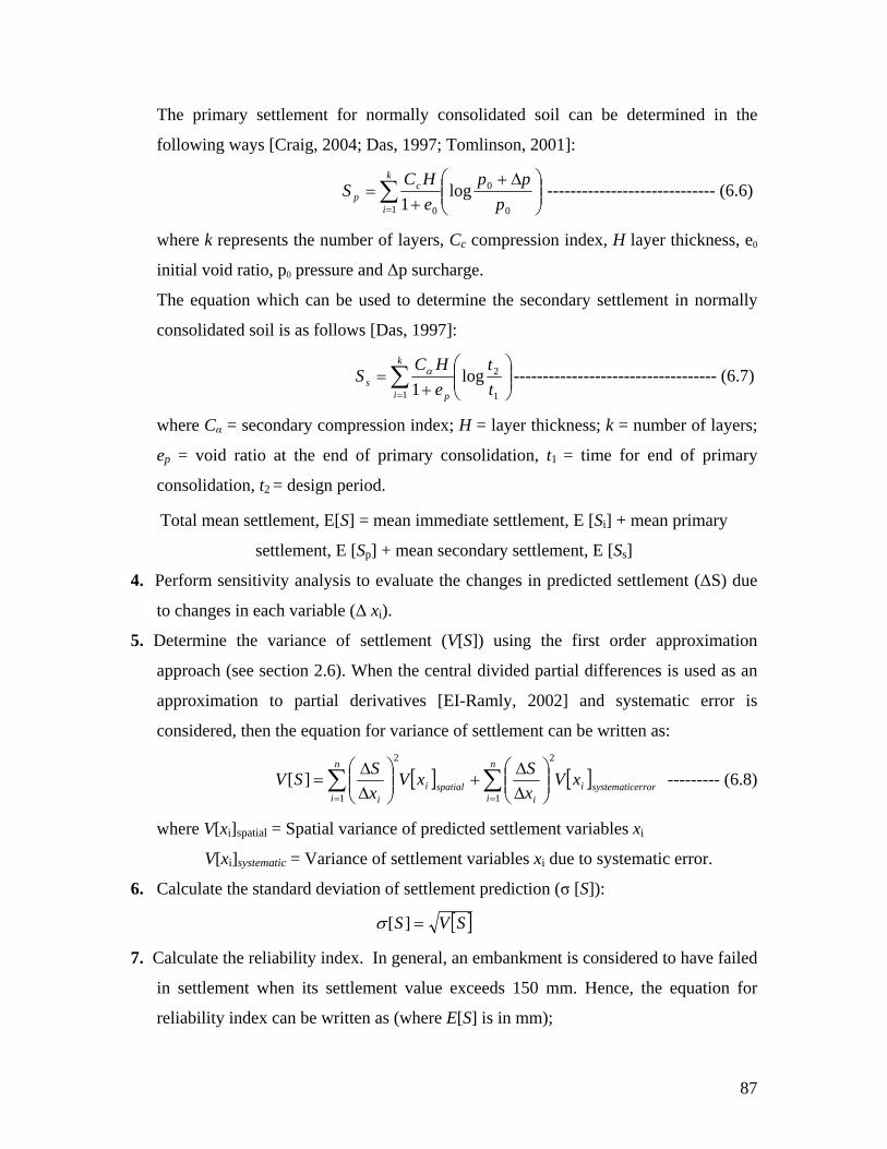
The primary settlement for normally consolidated soil can be determined in the
following ways [Craig, 2004; Das, 1997; Tomlinson, 2001]:
⎟⎟⎠
⎞⎜⎛ Δ+
= 0 ppHCkc ⎜
⎝+∑= 01 0
log1 pe
Si
p ----------------------------- (6.6)
f layers, Cc com
ally
follows [Das, 1997]:
where k represents the number o pression index, H layer thickness, e0
initial void ratio, p0 pressure and Δp surcharge.
The equation which can be used to determine the secondary settlement in norm
consolidated soil is as
⎟⎟⎠
⎞⎜⎜⎝
⎛+
= ∑= 1
2
1log
1 tt
eHC
Sk
i ps
α ----------------------------------- (6.7)
where Cα = secondary compression index; H = layer thickness; k = number of layers;
ep = void ratio at ary
consolidation, t2 = design period.
Total mean settlem ean primary
settlem [Ss]
4. Perform sensitivity analysis to evalua ted settlement (ΔS) due
to changes in each variable (Δ xi).
5. Determine the var rder approximation
approach (see section 2.6 l differences is used as an
approximation to partial derivatives [EI-Ramly, 2002] and systematic error is
considered, then th tten as:
the end of primary consolidation, t1 = time for end of prim
ent, E[S] = mean immediate settlement, E [Si] + m
ent, E [Sp] + mean secondary settlement, E
te the changes in predic
iance of settlement (V[S]) using the first o
). When the central divided partia
e equation for variance of settlement can be wri
[ ] [ ] errorsystematici
nn SS22⎞⎛ Δ⎞⎛ Δ
i ispatiali
i i
xVx
xVx
SV11
][ ∑∑==
⎟⎟⎠
⎜⎜⎝ Δ
+⎟⎟⎠
⎜⎜⎝ Δ
= --------- (6.8)
w predicte
lement var
6. Calculate the standard deviation of settlement prediction (σ [S]):
here V[xi]spatial = Spatial variance of
V[xi]systematic = Variance of sett
d settlement variables xi
iables xi due to systematic error.
[ ]SVS][σ =
7. Calculate the reliability index. In general, an embankment is considered to have failed
reliability index can be written as (where E[S] is in mm);
in settlement when its settlement value exceeds 150 mm. Hence, the equation for
87
[ ][ ]S
SEσ
β −=
150 ----------------------------------------- (6. 9)
8. Determine the reliability of the embankment from the standard normal curve area
value of the reliability index
Inc
table for the corresponding (see Appendix E-1).
orporation of desired reliability in the design for settlement
To incorporate a desired reliability in the de1. sign against settlement requires the
desired reliability level is determined
from the standard normal curve area Table (Appendix E-1).
mean predicted settle
limiting value of the mean predicted settlement to be determined first. To this end, the
reliability index value corresponding to the
2. Then the limiting value of the ment for a desired reliability level
is determined with the reliability index value in the following ways:
From equation 6.9, [ ][ ]S
SEσ
β −=
150 or [ ][ ] ][150
SCOVSESE
∗−
=β
or, [ ] [ ][ ]SCOVSE
∗+=
β1 -----------------------------(6.1
efficient of the variation of settlement, COV [S] is
150 0)
Here, the co- determined by
It should be appreciated that the method proposed for calculating settlement of
embankment is based on various parameters derived from laboratory test
the calculation based on the proposed method is likely to be conservative compared to in-
situ ement tends to
take ded
h is based on in-situ
analyzing the data collected from a similar existing structure, using the procedure
described in steps 1-6 above.
3. Hence, an embankment should be designed such that its mean predicted settlement is
less than or equal to the maximum allowable value of mean predicted settlement as
determined above to obtain the desired reliability in the design against settlement.
ing. Therefore
settlement. In addition a significant percentage of embankment settl
place during construction. Taking these factors into account it could be conclu
that the reliability calculated should be normally lower than that whic
testing data.
88
6.4 Embankment risk for both slope stabil
If the reliability of embankment design against slope stability is found to be 80%, it
cha ned for
ents built with this design
emb
obt
Sin nt for slope stability or
and of probabilities.
o independent eve will both occur is
simply the product of their probabilities. Now, applying this rule, the overall probability
of success of an embankment design (embankment desi
chance of success in both slope stability and settlement can be calculated as follows:
embankm
settlement ------------------------------------------ (7.1)
P (A∩B) = P (A). P (B)
ere are three possible outcomes which could occur when pavement and embankment
risks are considered together, since each event is independent. These are:
1. Risk of pavement failure and failure in embankment stability
ity and settlement
means that if 100 embankments are built with this design then 80 of them will have the
nce of not experiencing slope failure. Similarly, if the embankment is desig
60% reliability against settlement, then 60 out of 100 embankm
will have the chance of not failing in settlement. So, the probability of obtaining an
ankment with no slope failure in its design life is 0.8 (80/100) and the probability of
aining an embankment with no settlement failure in its design life is 0.6 (60/100).
ce the probabilities of successful performance of embankme
settlement are independent events, the general risk of embankment for both slope stability
settlement can be calculated using special multiplication rules
According to this rule, the probability that tw nts
gn reliability) considering the
The probability of overall success of embankment design = Probability of success of
ent design for slope stability × Probability of success of embankment design for
Hence, the general risk of embankment design = (1- the overall probability of success of
embankment design) × 100%
6.5 Overall risk of pavement-embankment design system
As pavement performance is linked to embankment performance a simple approach is
needed to reflect this in computing the joint probability of failure and risk. According to
the theory of probabilities, if P(A) is the probability of event A and P(B) is the
probability of event B, then the joint probability of events A and B may be determined in
the following way:
Th
89
2. Risk of pavement failure and failure in embankment settlement
3. Risk of pavement failure, failure in embankment stability and failure in
embankment settlement.
For example, if the reliability of pavement design is 70%, the reliability of embankment
design against slope stability is 80% and the reliability of embankment design against
settlement is 60%, then the overall risk of the design system can be calculated in the
following way:
Overall design risk (3 cases)
1. Risk of pavement failure and failure in embankment stability
= [1- (0.7×0.8)] = 0.44 or 44%
2. Risk of pavement failure and failure in embankment settlement
= [1- (0.7×0.6)] = 0.58 or 58%
3. Risk of pavement failure and failure in embankment stability and settlement
= [1- (0.7×0.8×0.6)] = 0.664 or 66.4%
6.6 Summary
embankment design risk considering both slope stab
system
of analyzing slope stability r redefined criteria. The first
order second moment method satisfied all requirements as a suitable method for
method. The detailed
e chapter presented a methodology using special multiplication rules
design and the overall risk of
of the roads in
Ba
This chapter presented the development of a suitable process for quantifying
ility and settlement for the design
of Bangladesh. To this end, it considered first a comparison of existing methods
isk with respect to the some p
Bangladesh. Moreover, this is a widely used and well recognized
procedure involved in this method was also presented. Similarly a suitable method was
developed in this research to quantify the embankment settlement risk by reviewing the
existing literature. The first order second moment theory was used in developing the
method of settlement risk analysis. The detailed procedure for this method was also
described. Finally, th
of probabilities to quantify the overall risk of embankment
a pavement-embankment design system. The next chapter will consider an integrated
example of an overall risk quantification process with field test data of one
ngladesh.
90

Chapter 7 An Integrated Example
7.1 Intr
ied first and then the embankment design risk for slope
ent design risk is
ent design system is
7.2.1 Application example o
Quantification of variance in traffic prediction
oduction
This chapter considers an integrated example of the quantification of risk in the pavement
and embankment design system for Bangladesh, based on the concepts presented in
Chapters 5 and 6. The data collected from road N302 are chosen for this example. The
pavement design risk is quantif
stability and settlement is determined. Next, the overall embankm
calculated. Finally, the overall risk of a pavement embankm
determined.
7.2 Pavement design risk quantification
f proposed method
iction data of road N302 is summarized as follows: 1. The traffic pred
Annual Average Daily Traffic (AADT) = 9303
Percentage of heavy vehicles (trucks, buses) in the traffic mix = 51.44%
The proportion of different types of heavy vehicle with their equivalent axle load factors
as found by the traffic and axle load survey is shown below: Parameter Heavy Truck Medium
Truck Small Truck Large Bus Medium Bus
Front Rear1 Rear2 Front Rear Front Rear Front Rear Front Rear Percent of Axles, pi
1.62 1.62 1.62 19.43 19.43 4.87 4.87 11.12 11.12 12.14 12.14
EALF, Fi 0.368 5.960 5.775 0.148 7.205 0.014 0.233 0.145 0.816 0.011 0.097
2. The AADT considers the traffic in both directions. To estimate the traffic in the design
direction, the direction distribution was taken as 50%. There is only one lane in the
design direction. Hence, the lane distribution is 100%. The variance in directional
distribution and lane distribution can be ignored. Traffic growth rate (r) data were taken
from a previous research report [khan, 2005]. The data for the co-efficient of variation of
ADT, growth rate, percentage of trucks, axles per truck are assumed in this example since
91
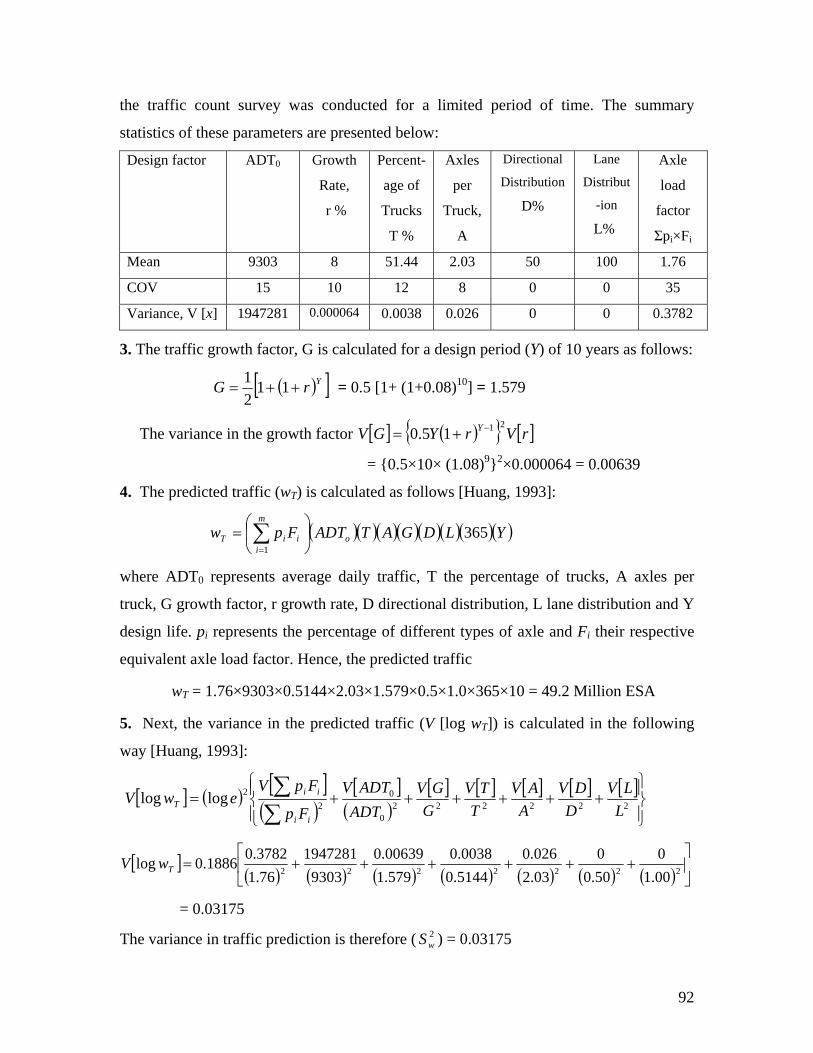
the traffic count s e. The summary
atistics of these parameters are presented below:
0 Growth
Rate,
Percent-
age of
Axles
per
Directional
Distribution Lane
DistributAxle
load
urvey was conducted for a limited period of tim
st
Design factor ADT
r % Trucks
T %
Truck,
A
D% -ion
L% factor
Σpi×Fi
Mean 9303 8 51.44 2.03 50 100 1.76
COV 15 10 12 8 0 0 35
Variance, V [x] 1947281 0.000064 0.0038 0.026 0 0 0.3782
3. The traffic growth factor, G is calculated for a design period (Y) of 10 years as follows:
( )[ ]YrG ++= 11 21 = 0.5 [1+ (1+0.08)10] = 1.579
The variance in the growth factor [ ] ( ){ } [ ]rVrYGV Y 2115.0 −+=
= {0.5×10× (1.08)9}2×0.000064 = 0.00639
lows [Huang, 1993]:
ks, A axles per
axle and Fi their respective
e axle l ence, th ed tr
wT = 1.76×9303×0.5144×2.03×1.579×0.5×1.0×365×10 = 49.2 Million ES
5 he an th V wT ca ed e w
w ng ]
4. The predicted traffic (wT) is calculated as fol
( )( )( )( )(DGATADTFpw oi
iiT1
⎟⎠
⎜⎝
= ∑=
m ⎞⎛ )( )( )( )YL 365
where ADT0 represents average daily traffic, T the percentage of truc
truck, G growth factor, r growth rate, D directional distribution, L lane distribution and Y
design life. pi represents the percentage of different types of
quivalent oad factor. H e ct predi affic
A
. Next, t vari ce in e predicted traffic ( [log ]) is lculat in th follo ing
ay [Hua , 1993 :
[ ] ( ) [ ]( )
[ ]( )
[ ] [ ] [ ] [ ] [ ]⎪⎭
⎪⎬⎫
⎪⎩
⎪⎨⎧
++++++=∑∑
2222220
02
2loglogL
LVD
DVA
AVT
TVG
GVADT
ADTVFp
FpVewV
ii
iiT
[ ]( ) ( ) ( ) ( ) ( ) ( ) ( ) ⎥
⎦
⎤⎢⎣
⎡++++++= 2222222 00.1
050.00
03.2026.0
5144.00038.0
579.100639.0
93031947281
76.13782.01886.0log TwV
= 0.03175
The variance in traffic prediction is therefore ( ) = 0.03175 2wS
92
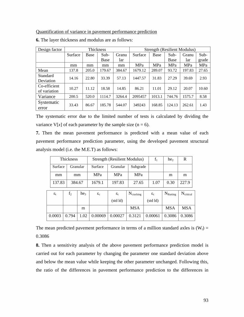
Quantification of variance in pavement performance prediction
6. The layer thickness and modulus are as follows:
Th tre ient lus) Design factor ickness S ngth (Resil Modu Surface Base - S e b
Base u
r Sub
Base Granu
lar urfac Base Su - Gran
laSub-grade
mm mm MPa MPa mm mm MPa MPa MPa Mean 137.8 205.0 179.67 16 289.07 93.72 7.83 384.67 79.12 19 27.65 Standard Deviation 14 22.80 .39 1 31. 27.29 .69 .16 33 57.13 447.57 83 39 2.93
Co-efficient 10.2 11.12 .58 1 8 1 11. 29.12 0.07 of variation 7 18 4.85 6.2 01 2 10.60
Variance 2 0. 2 101 744.76 75.7 00.5 52 0 1114.7 3264.4 095457 3.1 15 8.58 Systematic error 33.43 86.67 185.78 544.07 349243 168.85 124.13 262.61 1.43
error due to the ulated by dividing the
variance V[x] of each parameter by the sample size (n = 6).
rmance is predicted with a mean value of each
uctural
ickness Strength (Resilient Modulus) he2 R
The systematic limited number of tests is calc
7. Then the mean pavement perfo
pavement performance prediction parameter, using the developed pavement str
analysis model (i.e. the M.E.T) as follows:
Th f1
Surface Granular Surface Granular Subgrade
mm mm MPa MPa MPa m m
137.83 384.67 1679.1 197.83 27.65 1.07 0.30 227.9
εt f2 he3 εc εt (std ld)
Ncracking ε N N c
(std ld) Rutting critical
m MSA MSA MSA
0.0003 0.794 1.02 0.00069 0.00027 0.3121 0.00061 0.3086 0.3086
The mean predicted pavement performance in terms of a million standard axles is (Wt) =
8. Then a sensitivity analysis of the above pavement performance prediction model is
carried out for each parameter by changing the parameter one standard deviation above
and below the mean value while keeping the other parameter unchanged. Following this
the ratio erences in pavement performance prediction to the differences in
0.3086
,
of the diff
93
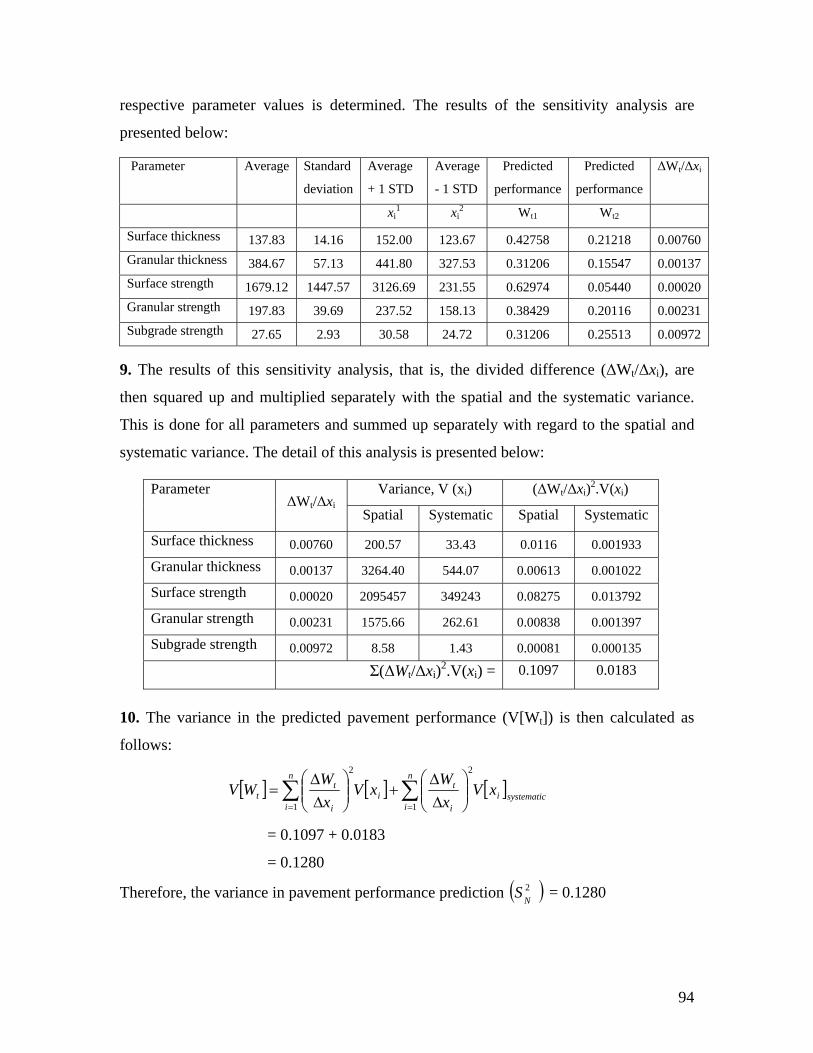
respective parameter values is determined. The results of the sensitivity analysis are
Average
iat
Average
1
Average
- pe nce fo
ΔW /Δxi
presented below:
Parameter Standard
dev ion + STD
Predicted Predicted
1 STD rforma per rmance t
x Wi1 xi
2 Wt1 t2
Surface thickness .83 . 1 2 137 14 16 52.00 123.67 0.42758 0. 1218 0.00760Granular thickness .67 .1 44 6 15 0 7 384 57 3 1.80 327.53 0.3120 0. 547 .0013Surface strength .1 7 31 2 4 05 1679 2 144 .57 26.69 31.55 0.6297 0. 440 0.00020Granular strength 83 .6 23 20 0.197. 39 9 7.52 158.13 0.38429 0. 116 00231 Subgrade strength 27.65 2.93 30.58 24.72 0.31206 0.25513 0.00972
sensitivity analysis, that is, the divided difference (ΔW /Δx ), are
ith regard to the spatial and
iance, V (xi) (ΔWt/Δxi)2.V(xi)
9. The results of this t i
then squared up and multiplied separately with the spatial and the systematic variance.
This is done for all parameters and summed up separately w
systematic variance. The detail of this analysis is presented below:
VarParameter ΔWt/Δxi
Spatial Systematic Spatial Systematic
Surface thickness 0.0 0.0116 0.00 33 0760 200.57 33.43 19
Granular thickness 0.0 326 5 00613 0.0 22 0137 4.40 44.07 0. 010
Surface strength 0.0 20 27 0 0020 95457 349243 0.08 5 .013792
Granular strength 0.00231 1575.66 262.61 0.00838 0.001397
Subgrade strength 009 5 00. 72 8. 8 1.43 0.00 81 0.000135
Δxi)2.V(xi) 097 0.0183 Σ(ΔWt/ = 0.1
10. Th n th a e t] n ated as
e varia ce in e predicted p vement p rformance (V[W ) is the calcul
follows:
[ ] [ ] [ ]systematici
n
i ii i xx 11 == ⎠⎝ Δ⎠⎝ Δ
= 0.1097 + 0.0183
= 0.1280
Therefore, the variance in pavement performance prediction
ti
nt
t xVW
xVW
WV ∑∑ ⎟⎟⎞
⎜⎜⎛ Δ
+⎟⎟⎞
⎜⎜⎛ Δ
= 22
( )2N
S = 0.1280
94
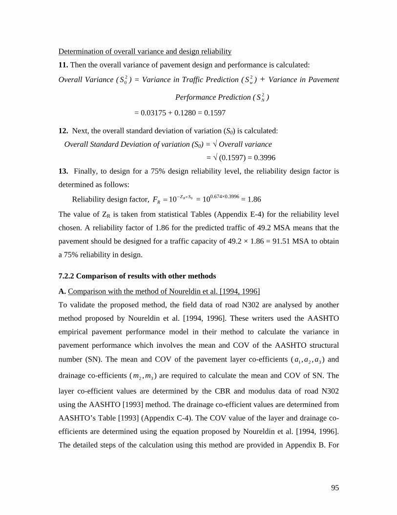
Determination of overall variance and design reliability
11. Then the overall variance of pavement design and performance is calculated:
Overall Variance ( n P aria av
Performance Prediction (
.03 0.1 0.1
1 ra ard tion ati is c d:
ard n at ll v
= √
Finally, to design for a 75% design reliability level, the reliability design factor is
eans that the
pave ld be desig traff .2 × 1.8 to obtain
a 75% reliability in design.
7.2.2 esu ot hods
A. C the m N et a , 199
20S ) = Variance i Traffic rediction ( 2
wS ) + V2S )
nce in P ement
N
= 0 175 + 280 = 597
2. Next, the ove ll stand devia of vari on (S0) alculate
Overall Stand Deviatio of vari ion (S0) = √ Overa ariance
(0.1597) = 0.3996
13.
determined as follows:
Reliability design factor, 010 SZR
RF ×−= = 100.674×0.3996 = 1.86
The value of ZR is taken from statistical Tables (Appendix E-4) for the reliability level
chosen. A reliability factor of 1.86 for the predicted traffic of 49.2 MSA m
ment shou ned for a ic capacity of 49 6 = 91.51 MSA
Comparison of r lts with her met
omparison with ethod of oureldin l. [1994 6]
To v sed , th ata of road N302 are analysed by another
method proposed by Noureldin et al. [1994, 1996]. These writers used the AASHTO
empirical pavement performance mo to ate ance in
SN). The mean and COV of the pavement layer co-efficients ( ) and
drainage co-efficients ( ) are required to calculate the m
values are determined by the CBR and modulus data of road N302
ainage co-efficient values are determined from
dix C-4). The COV value of the layer and drainage co-
ourel 994, 1996].
The detailed steps of the calculation using this method are provided in Appendix B. For
alidate the propo method e field d
del in their method calcul the vari
pavement performance which involves the mean and COV of the AASHTO structural
number ( 321 ,, aaa
ean and COV of SN. The 32 ,mm
layer co-efficient
using the AASHTO [1993] method. The dr
AASHTO’s Table [1993] (Appen
efficients are determined using the equation proposed by N din et al. [1
95
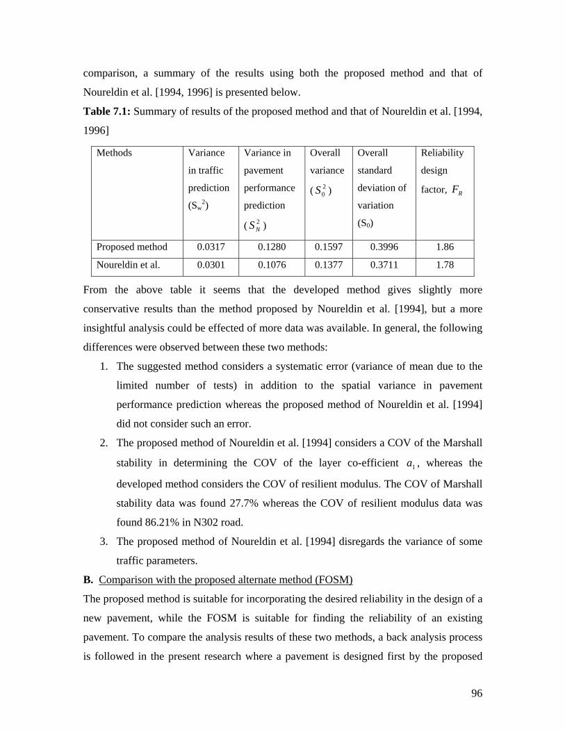
comparison, a summary of the results using both the proposed method and that of
1996]
in traffic pavement
rall
variance
Overall
standard
f
Reliability
design
factor,
Noureldin et al. [1994, 1996] is presented below.
Table 7.1: Summary of results of the proposed method and that of Noureldin et al. [1994,
Methods Variance Variance in Ove
prediction performance ( 20S ) deviation o
RF (Sw
2) prediction variation
( 2NS ) (S0)
Proposed method 0.0317 0.1280 0.1597 0.3996 1.86
Noureldin et al. 0.0301 0.1076 0.1377 0.3711 1.78
From the above table it s he developed methodeems that t gives slightly more
considers a systematic error (variance of mean due to the
the spatial variance in pavement
Noureldin et al. [1994]
found 86.21% in N302 road.
ethod of Nourel
conservative results than the method proposed by Noureldin et al. [1994], but a more
insightful analysis could be effected of more data was available. In general, the following
differences were observed between these two methods:
1. The suggested method
limited number of tests) in addition to
performance prediction whereas the proposed method of
did not consider such an error.
2. The proposed method of Noureldin et al. [1994] considers a COV of the Marshall
stability in determining the COV of the layer co-efficient 1a , whereas the
developed method considers the COV of resilient modulus. The COV of Marshall
stability data was found 27.7% whereas the COV of resilient modulus data was
3. The proposed m din et al. [1994] disregards the variance of some
traffic parameters.
B. Comparison with the proposed alternate method (FOSM)
The proposed method is suitable for incorporating the desired reliability in the design of a
new pavement, while the FOSM is suitable for finding the reliability of an existing
pavement. To compare the analysis results of these two methods, a back analysis process
is followed in the present research where a pavement is designed first by the proposed
96
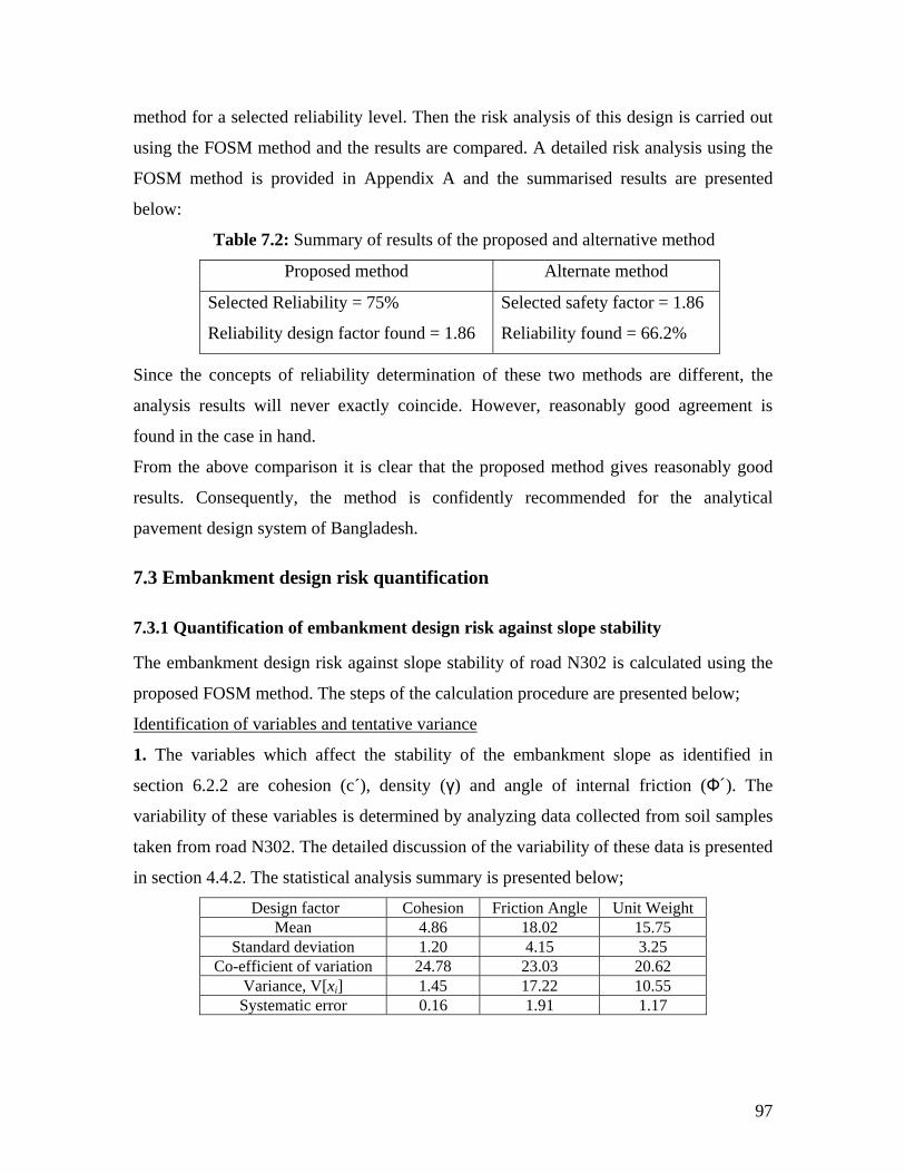
method for a selected reliability level. Then the risk analysis of this design is carried out
using the FOSM method and the results are compared. A detailed risk analysis using the
S of pr an tive m
Pr eth te thod
FOSM method is provided in Appendix A and the summarised results are presented
below:
Table 7.2: ummary
oposed m
results of the
od
oposed
Al
d alterna
rnate me
ethod
Selected Reliability = 75%
Reliability design factor found = 1.86
el ted s =
Reliability found = 66.2%
S ec afety factor 1.86
Since the concepts of reliability determ tion of these two methods are different, the
an l nev tly co How ason od ag
found in the case in hand.
ility of road N302 is calculated using the
culation procedure are presented below;
ina
alysis results wil er exac incide. ever, re ably go reement is
From the above comparison it is clear that the proposed method gives reasonably good
results. Consequently, the method is confidently recommended for the analytical
pavement design system of Bangladesh.
7.3 Embankment design risk quantification
7.3.1 Quantification of embankment design risk against slope stability
The embankment design risk against slope stab
proposed FOSM method. The steps of the cal
Identification of variables and tentative variance
1. The variables which affect the stability of the embankment slope as identified in
section 6.2.2 are cohesion (c´), density (γ) and angle of internal friction (Ф´). The
variability of these variables is determined by analyzing data collected from soil samples
taken from road N302. The detailed discussion of the variability of these data is presented
r Cohesion Friction Angle Unit Weight
in section 4.4.2. The statistical analysis summary is presented below;
Design factoMean 4.86 18.02 15.75
Standard deviation 1.20 4.15 3.25 Co-efficient of variation 24.78 23.03 20.62
Variance, V[xi] 1.45 17.22 10.55 Systematic error 0.16 1.91 1.17
97
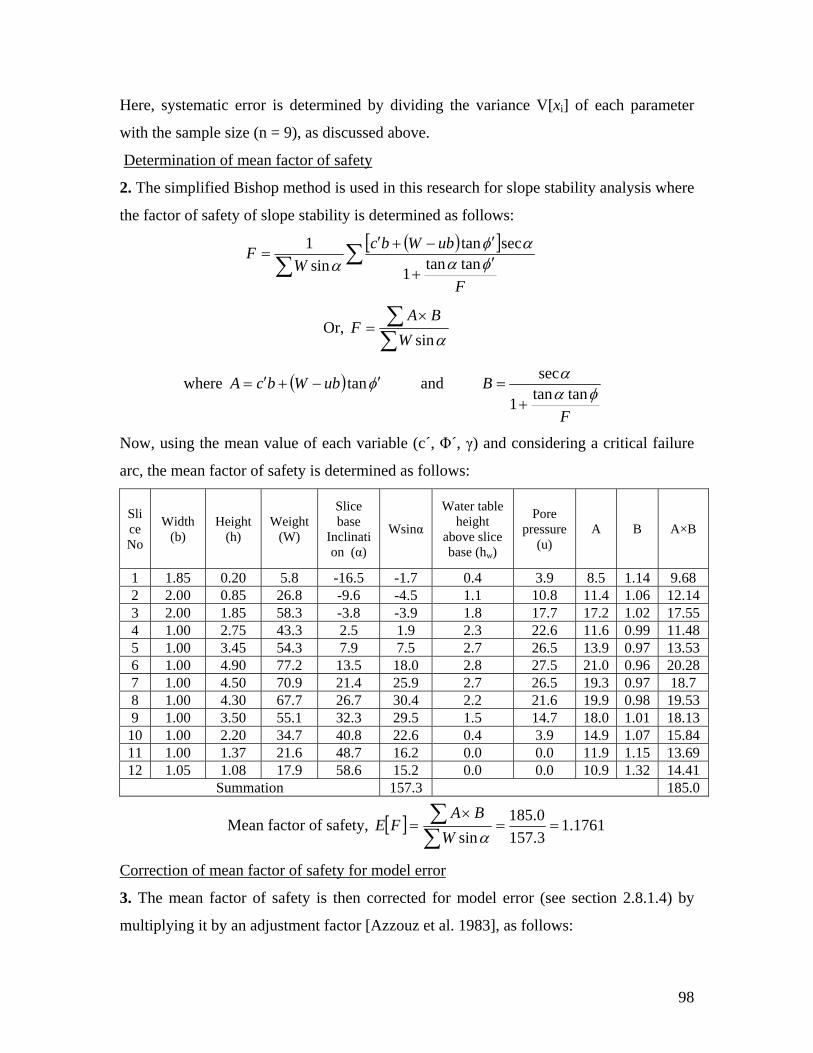
Here, systematic error is determined by dividing the variance V[xi] of each parameter
with the sample size (n = 9), as discussed above.
Determination of mean factor of safety
2. The simplified Bishop method is used in this research for slope stability analysis where
the factor of safety of slope stability is determined as follows:
( )[ ]∑∑ ′+
′+ −′=
c
F
ubWbFW φα
αφαsin tantan1
tan sec 1
Or, ∑∑ × BA
=αsinW
F
where ( ) φ ′−+′= tanubWbcA and Bφα
α
Ftantan1+
=
d as follows:
No (b) (h) (W)
sec
Now, using the mean value of each variable (c´, Φ´, γ) and considering a critical failure
arc, the mean factor of safety is determine
Slice Width Height Weight
Slice base Wsinα
Water ta
Inclinati
ble height
above slice
Pore pressure
(u) A B A×B
on (α) base (hw)
1 1.85 0.20 5.8 -16.5 -1.7 0.4 3.9 8.5 1.14 9.68 2 2.00 0.85 26.8 -9.6 -4.5 1.1 10.8 11.4 1.06 12.14 3 2.00 1.85 58.3 -3.8 -3.9 1.8 17.7 17.2 1.02 17.55 4 1.00 2.75 43.3 2.5 1.9 2.3 22.6 11.6 0.99 11.48 5 1.00 3.45 54.3 7.9 7.5 2.7 26.5 13.9 0.97 13.53 6 1.00 4.90 77.2 13.5 18.0 2.8 27.5 21.0 0.96 20.28 7 1.00 4.50 70.9 21.4 25.9 2.7 26.5 19.3 0.97 18.7 8 1.00 4.30 67.7 26.7 30.4 2.2 21.6 19.9 0.98 19.53 9 1.00 3.50 55.1 32.3 29.5 1.5 14.7 18.0 1.01 18.13
10 1.00 2.20 34.7 40.8 22.6 0.4 3.9 14.9 1.07 15.84 11 1.00 1.37 21.6 48.7 16.2 0.0 0.0 11.9 1.15 13.69 12 1.05 1.08 17.9 58.6 15.2 0.0 0.0 10.9 1.32 14.41
Summation 157.3 185.0
[ ] 1761.1=3.1570
s.185×
in== Mean factor of safety,
∑∑
αW
Correction for error
BAFE
of mean factor of safety model
3. The mean factor of safety is then corrected for m rror (see n 2.8.1.4) by
multiplying it by an adjustment factor [Azzouz et al. 1983], as follows:
odel e sectio
98
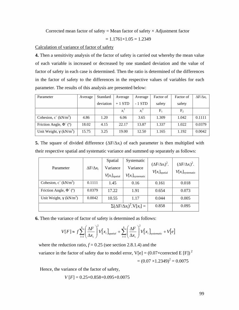
Corrected mean factor of safety = Mean factor of safety × Adjustment factor
= 1.1761×1.
05 = 1.2349
yCalculation of variance of factor of safet
eviation and the value of
ch case is determined. Then the ratio is determined of the differences
in the factor of safety to the differences in the respective values of variables for each
parameter. The results of this analysis are presented below:
dard
deviation
Average
+ 1 STD
Average
- 1 STD
Factor of
safety
Factor of
safety
ΔF/Δxi
4. Then a sensitivity analysis of the factor of safety is carried out whereby the mean value
of each variable is increased or decreased by one standard d
factor of safety in ea
Parameter Average Stan
xi1 xi 2 F1 F2
Cohesion, c´ (kN/m2) 4.86 1.20 6.06 3.65 1.309 1.042 0.1111
Friction Angle, Ф´ (º) 18.02 4.15 22.17 13.87 1.337 1.022 0.0379
Unit Weight, γ (kN/m3) 15.75 3.25 19.00 12.50 1.165 1.192 0.0042
5. The square of divided difference (ΔF/Δxi) of each parameter is then multiplied with
t r v l tem iance an p tely as follows:
ame Δx
atial
rian
[xi]sp
Sy
Vari
V[xi]sy c
(ΔF/Δxi)2.
V[ al (ΔF/Δxi)2.
i ic
heir especti e spatia and sys atic var
Sp
d summed u
stematic
separa
Par ter ΔF/ i Va ce
V atial ance
stematix ]i spati V[x ]systemat
Coh ´ (k 11 1.45 0.16 0esion, c N/m )2 0.11 0.161 .018
Frict gle 79 17.22 1. 0ion An , Ф´ (º) 0.03 91 0.654 .073
Unit Weight, γ 3) 42 1. 0 (kN/m 0.00 10.55 17 0.044 .005
Σ( xi)2.V 0ΔF/Δ [xi] = 0.858 .095
6 en ar of f of s is d ined llows:
. Th the v iance actor afety eterm as fo
[ ] [ ] [ ]eVxVxFxV
xFfF ≈ ∑][V systemai
i ispatii
i i
+⎟⎟⎠
⎜⎜⎝
⎛ΔΔ
⎟⎟⎠
⎞⎜⎜⎝ Δ == 1
2
1
section 2.8.1.4) and the 2
2
V [F] = 0.25×0.858+0.095+0.0075
tic
k
al +∑k ⎛ Δ ⎞
2
where the reduction ratio, f = 0.25 (see
variance in the factor of safety due to model error, V[e] = (0.07×corrected E [F])
= (0.07 ×1.2349) = 0.0075
Hence, the variance of the factor of safety,
99
= 0.3175
Determination of reliability index
7. The reliability index (β) is then calculated using the following equation:
[ ][ ]F
FEσ
β 0.1−=
where the mean factor of safety, E [F] = 1.1761
The standard deviation of factor of safety, σ [F] = √ V [F] = √0.3175 = 0.5634, hence
Rel n iability i dex,5634.0
11761. 0.1 −=β
= 0.31
D sk of 2 roa bank agai ope y
3
etermination of Ri N30 d em ment nst sl stabilit
8 rd l curve area [A x E e rel y o
e in the spon alu e re y ind
Incorporation of the desired reliability gn ability
. From the standa norma Table ppendi -1], th iabilit f the
mbankment is determ ed for corre ding v e of th liabilit ex.
The reliability of N302 road embankment is found to be 63%
Hence, the risk of embankment failure in slope stability = 1 - 63% = 37%
in desi for slope st
9. The required value of th fa fety to achieve eli l in
design against slope stability is deter n .4 llow
e mean ctor of sa
mined usi
a desired r
in the fo
ability leve
ing way: g Equation 6
[ ] [ ]][ FVCOF
∗=
1
wh ete fro ana results n exis imilar
embankment. The COV [F] for N302 ro follo
E− β1
ere COV [F] is d rmined m the lysis of a ting s
ad is determined as ws:
[ ] [ ] [ ] 9.471001761.15634.0100 =×=×=
FEFFCOV σ %
index, β is determined from the standard normal curve area Table
[Appendix E-1]. For the desired reliability level of 80%, the value of reliability index, β =
The reliability
0.842
Hence, the required value of the mean factor of safety,
[ ][ ][ ] [ ] 675.1479.0841.01
111 ∗−
=FCOV
FEβ
=×−
=
100
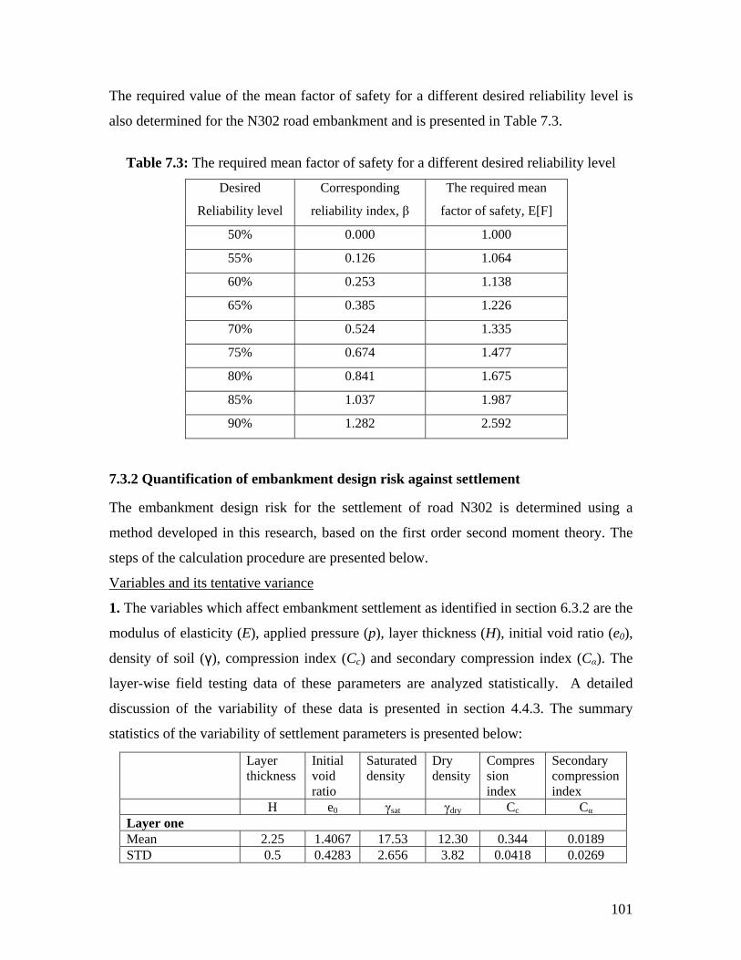
The required value of the mean factor of safety for a different desired reliability level is
lso determined for the N302 road embankment and is presented in Table 7.3.
bility level
Desired Corresponding
eliability index,
The required mean
factor of safety, E[F]
a
Table 7.3: The required mean factor of safety for a different desired relia
Reliability level r β
50% 0.000 1.000
55% 0.126 1.064
60% 0.253 1.138
65% 0.385 1.226
70% 0.524 1.335
75% 0.674 1.477
80% 0.841 1.675
85% 1.037 1.987
90% 1.282 2.592
7.3.2 Quantification of embankment design risk against settlement
The
steps of the calculation procedure are presented below.
ce
The embankment design risk for the settlement of road N302 is determined using a
method developed in this research, based on the first order second moment theory.
Variables and its tentative varian
itial void ratio (e0),
density of soil (γ), compression index (Cc) and secondary compression index (Cα). The
data of these parameters are analyzed statistically. A detailed
Layer thickness
Initial void
Saturated density
Dry density
Compression index
Secondary compression index
1. The variables which affect embankment settlement as identified in section 6.3.2 are the
modulus of elasticity (E), applied pressure (p), layer thickness (H), in
layer-wise field testing
discussion of the variability of these data is presented in section 4.4.3. The summary
statistics of the variability of settlement parameters is presented below:
ratio H e0 γsat γdry Cc Cα Layer one Mean 2.25 1.4067 17.53 12.30 0.344 0.0189 STD 0.5 0.4283 2.656 3.82 0.0418 0.0269
101
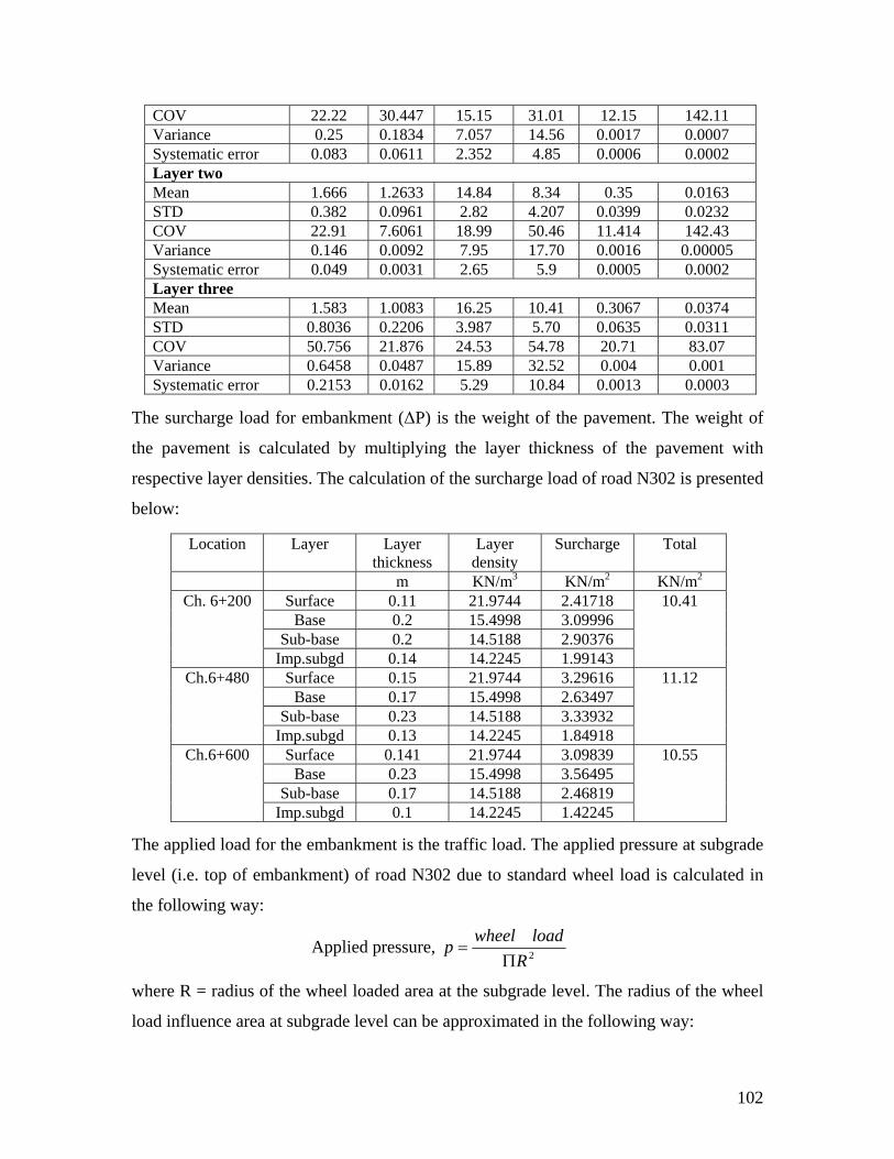
COV 22.22 30.447 15.15 31.01 12.15 142.11 Variance 0.25 0.1834 7.057 14.56 0.0017 0.0007 Systematic error 0.083 0.0611 2.352 4.85 0.0006 0.0002 Layer two Mean 1.666 1.2633 14.84 8.34 0.35 0.0163 STD 0.382 0.0961 2.82 4.207 0.0399 0.0232 COV 22.91 7 5 142.43 .6061 18.99 0.46 11.414 Variance 0.00005 0.146 0.0092 7.95 17.70 0.0016 Systematic error 0.049 0.0031 2.65 5.9 05 0.0002 0.00Layer three Mean 1.583 1.0083 5 10.41 67 0.0374 16.2 0.30STD 0.8036 0.2206 7 5.70 35 0.0311 3.98 0.06COV 50.756 21.876 3 54.78 1 83.07 24.5 20.7Variance 0.6458 0.0487 9 32.52 4 0.001 15.8 0.00Systematic error 53 0.0162 5.29 10.84 13 0.0003 0.21 0.00
The surcharge load bankment (Δ he weight of the ent. The weight of
the pavement is ca ed by multiplying the layer thickne the pavement with
respective layer den The calculatio e surcharge load of road N302 is presented
below:
Location Layer Layer thickness
Layer density
Surcharge Total
for em P) is t pavem
lculat ss of
sities. n of th
m KN/m3 KN/m2 KN/m2 Surface 0.11 21.9744 2.41718
Base 0.2 15.4998 3.09996 Sub-base 0.2 14.5188 2.90376
Ch. 6+200
Imp.subgd 0.14 14.2245 1.99143
10.41
Surface 0.15 21.9744 3.29616 Base 0.17 15.4998 2.63497
Sub-base 0.23
Ch.6+480
14.5188 3.33932 Imp.subgd 0.13 14.2245 1.84918
11.12
Surface 0.141 21.9744 3.09839 Base 0.23 15.4998 3.56495
Sub-base 0.17 14.5188 2.46819
Ch.6+600
Imp.subgd 0.1 14.2245 1.42245
10.55
The applied load for the embankment is the traffic load. The applied pressure at subgrade
level (i.e. top of embankment) of road N302 due to standard wheel load is calculated in
ollowing way:
Applied pressure,
the f
2Rloadwhp eel
Π=
where R = radius of the wheel loaded area at the subgrade level. The radius of the wheel
load influence area at subgrade level can be approximate e f g wad in th ollowin y:
102
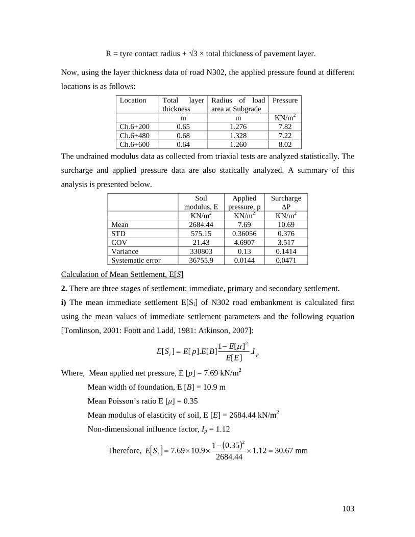
R = tyre co to kne ave ayer.
Now, using the layer thickness data of road N e a pre und rent
locations is as follows:
Locatio ota r hick Sub
P
ntact radius + √3 × tal thic ss of p ment l
302, th pplied ssure fo at diffe
n T l layet ness
Radius of load area at grade
ressure
m m KN/m2 Ch.6+2 1.276 00 0.65 7.82 Ch.6+480 0.68 1.328 7.22 Ch.6+6 0 00 0.64 1.26 8.02
The undrained modulus data as col rom al te
sur d applied d als call yze ummary of this
lected f triaxi sts are analyzed statistically. The
charge an pressure ata are o stati y anal d. A s
analysis is presented below.
Soil modulus, E
Applied pressure, p
Surcharge ΔP
KN/m2 KN/m2 KN/m2 Mean 2684.44 7.69 10.69 STD 575.15 0.36056 0.376 COV 21.43 4.6907 3.517 Varianc 803 .13 e 330 0 0.1414 Systematic error 5.9 44 0.0471 3675 0.01
Calcula an S nt, E[Stion of Me ettleme ]
2. There are three stage ettlement: immedia ry a ary set ment.
i) The mean immediate settlement of N em
using t alue mediate settlemen ters and the following equation
[Tomlinson, 2001: Foott and Ladd, 1981: Atkinson, 2007]:
s of s te, prima nd second tle
E[Si] 302 road bankment is calculated first
he mean v s of im t parame
pi IEE ][
E ][1 μ−BES .][][2
Where, Mean appli ure, = 7.69
s of elasticity of soil, E [E] = 2684.44 kN/m
Non-dimensional influence factor, Ip = 1.12
Therefore,
pE ].[=E
ed net press E [p] kN/m 2
Mean width of foundation, E [B] = 10.9 m
Mean Poisson’s ratio E [μ] = 0.35
Mean modulu 2
[ ] ( )=×
−××= 12.1
44.2684i35.019.1069.7
2
SE 30.67 mm
103
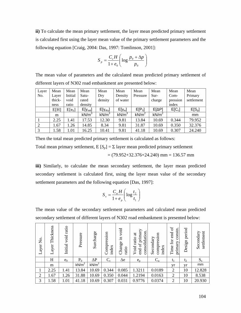
ii) To calculate the mean primary settlement, the layer mean predicted primary settlement
ig, 2004: Das, 1997: Tomlinson, 2001]:
is calculated first using the layer mean value of the primary settlement parameters and the
following equation [Cra
⎟⎟⎠
⎞Δ+0ogp
pp ⎜⎜
⎛+
= l1
HCS c
p⎝0e
The mean value ted redicted ary settlement of
different layers of N302 road emba nt are presented below:
index
0
of parameters and the calcula mean p prim
nkmeLayer No.
Mean Layer thick-ness
Mean Initial void ratio
Mean Satu-rated density
Mean Dry density
Mean Density of water
Mean Pressure
Mean Sur-charge
Mean Com-pression
Mean Primary settlement
E[H] E[e0] E[γsat] E[γdry] E[γw] E[P0] E[ΔP] E[Cc] E[Sp] m kN/m3 kN/m3 kN/m3 kN mm kN/m2 /m2
1 2.25 1.41 17.53 12.3 10.69 0.344 79.952 0 9.81 13.84 2 1.67 1.26 14.85 8.34 10. 350 32.376 9.81 31.87 69 0.3 1.58 16.25 10.41 4 10.6 .307 24.240 1.01 9.81 1.18 9 0
Then the total m redicted primary s nt is d as f :
Total mean prim ement, E [Sp] = mean cted p ettlement
= +32.3 .240) 36.57 mm
ed
ean p e ettlem c ealculat ollows
ary settl Σ layer predi rimary s
(79.952 76+24 mm = 1
iii) Similarly, to calculate the mean secondary settlement, the layer mean predict
secondary settlement is calculated first, using the layer mean value of the secondary
settlement parameters and the following equation [Das, 1997]:
⎟⎟⎞
⎜⎜⎛
= 2log tHCSs
α ⎠⎝+ 11 tep
The mean value of the secondary settlement parameters and calculated mean predicted
bankment is presented below:
inde
x
Tim
e fo
r end
of
prim
ary
cons
tn.
Des
ign
perio
d
Seco
ndar
y se
ttlem
ent
secondary settlement of different layers of N302 road em
Laye
r No.
Laye
r Thi
ckne
ss
Initi
al v
oid
ratio
Pres
sure
Surc
harg
e
Com
pres
sion
Cha
nge
in v
o
Voi
d ra
tio a
t en
d of
prim
ary
cons
olid
atio
n.
Seco
ndar
y co
mpr
essi
on id
inde
x
ratio
H ΔP Cc Δe ep Cα t2 Ss e0 P0 t1 m kN/m2 yr mm kN/m2 yr 1 2.25 1.41 13.84 10.69 0.344 0.085 1.3211 0.0189 2 10 12.828 2 1.67 1.26 31.88 10.69 0.350 0.044 1.2194 0.0163 2 10 8.538 3 1.58 1.01 41.18 10.69 0.307 0.031 0.9776 0.0374 2 10 20.930
104
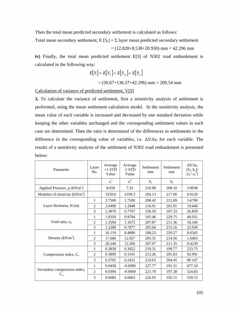
Then the total mean predicted secondary settlement is calculated as follows:
Total mean secondary settlement, E [Ss] = Σ layer mean predicted secondary settlement
= (12.828+8.538+20.930) mm = 42.296 mm
dicted settlement E[S] of N302 road embankment is
calculated in the following way:
iv) Finally, the total mean pre
[ ] [ ] [ ] [ ]spi SESESESE ++=
= (30.67+136.57+42.296) mm = 209.54 mm
C t v e dic ttle V[Salcula ion of arianc of pre ted se ment, ]
3. To c te va of e a sensitiv ly t
performe n tle alc m In ns anal e
m a re o da iati le
k ping he iab cha and or ding settlem lue h
e are ined. Then the rat eter d o iffe in me
variable. The
nted
alcula the riance settlem nt, first ity ana sis of se
i
tlement is
d, usi g the mean set ment c ulation odel. the se tivity ysis, th
ean value of each variable is increased nd dec ased by ne stan rd ev d o in wh
ee the ot r var les un nged the c respon ent va s in eac
cas determ io is d mine f the d rences settle nts to the
difference in the corresponding value of variables, i.e. ΔS/Δxi for each
results of a sensitivity analysis of the settlement of N302 road embankment is prese
below:
Parameter Layer No.
Average +1 STD Value
Average -1 STD Value
Settlement mm
Settlement mm
ΔS/Δxi [S1-S2]/ [xi
1-xi2]
xi1 xi
2 S1 S2 Applied Pressure, p (kN/m2) 8.050 7.33 210.98 208.10 3.9938
Modulus of elasticity (kN/m2) 3259.6 2109.3 204.13 217.90 0.0120 1 2.7500 1.7500 208.42 212.09 3.6700 2 2.0490 1.2848 216.91 201.91 19.640 Layer thickness, H (m) 3 2.3870 0.7797 230.50 187.33 26.859 1 1.8350 0.9784 195.46 229.75 40.031 2 1.3594 1.1672 207.87 211.36 18.160 Void ratio e0
2289 0.7877 05.04 22.,
3 1. 2 215.16 939 1 16.119 8.4 8.6 880 184.23 250.27 545 2 17.666 12. 1.6 027 205.31 214.56 403 Density ( m3)
0 . 0.4kN/
3 20.24 12 266 207.97 211.35 239 1 8 3 233.75 0.385 0. 022 219.31 199.77 2 0.3899 3101 213. 20 3 92.990. 26 5.8 1 Com ssion ex, C
02 2 2 2 6 2 5 80.1pre ind c
3 0.37 0. 43 14. 3 04.4 47 1 0.0458 .0 22 19 1 67 -0 080 7.77 1.3 7.54 2 0.0394 .0 22 19 8 524. -0 069 1.70 7.3 83 Secon om on
C5 00 22 19 5 55
dary c pressi
index, α
3 0.068 0. 63 6.93 2.1 9.72
105
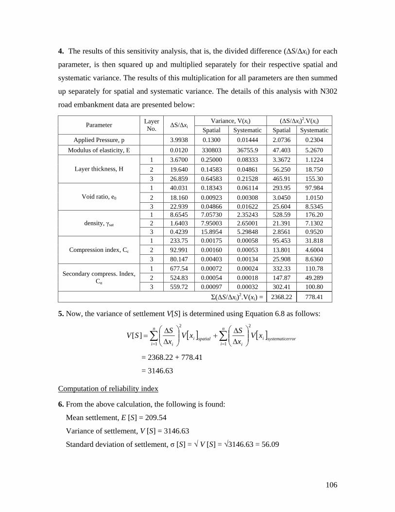
4. The results of this sensitivity analysis, that is, the divided difference (ΔS/Δxi) for each
ed
ed below:
Variance, V(xi) (ΔS/Δxi)2.V(xi)
parameter, is then squared up and multiplied separately for their respective spatial and
systematic variance. The results of this multiplication for all parameters are then summ
up separately for spatial and systematic variance. The details of this analysis with N302
road embankment data are present
Parameter LaNo
yer . ΔS/Δxi Spatial Systematic Spatial Systematic
Applied Pressure, p 3.9938 0.1300 0.01444 2.0736 0.2304 Modulus of elasticity, E 0.0120 330803 36755.9 47.403 5.2670
1 3.6700 0.25000 0.08333 3.3672 1.1224 2 19.640 0.14583 0.04861 56.250 18.750 Layer thickness, H 3 26.859 0.64583 0.21528 465.91 155.30 1 40.031 0.18343 0.06114 293.95 97.984 2 18.160 0.00923 0.00308 3.0450 1.0150 Void ratio, e0 3 22.939 0.04866 0.01622 25.604 8.5345 1 8.6545 7.05730 2.35243 528.59 176.20 2 1.6403 7.95003 2.65001 21.391 7.1302 density, γsat 3 0.4239 15.8954 5.29848 2.8561 0.9520 1 233.75 0.00175 0.00058 95.453 31.818 2 92.991 0.00160 0.00053 13.801 4.6004 Compression index, Cc 3 80.147 0.00403 0.00134 25.908 8.6360 1 677.54 0.00072 0.00024 332.33 110.78 2 5 0 424.83 .00054 0.00018 147.87 9.289 Secondary compress. Index,
5 0. 0.0 30 1Cα
3 59.72 00097 0032 2.41 00.80 Σ S/Δxi)2.V(x ) = 2368 22 778.41 (Δ i .
5. tlem V[ eterm usin ion ollo
Now, the variance of set ent S] is d ined g Equat 6.8 as f ws:
] [xV⎟⎟⎞[ ]systispat
n
i i xS
xSSV ][ ∑
=⎜⎜⎝
⎛ΔΔ
ΔΔ
=
= 2368.22 + 778.41
= 3146.63
Computation of reliability inde
errorematic
n
i 1= i ⎠ial ∑+ixV⎟⎟
⎞22
1 ⎝ ⎠⎜⎜⎛
x
6. From the above calculation, the following is found:
Mean settlement, E [S] = 209.54
Variance of settlement, V [S] 314
lem σ V 314 56.0
= 6.63
Standard deviation of sett ent, [S] = √ [S] = √ 6.63 = 9
106
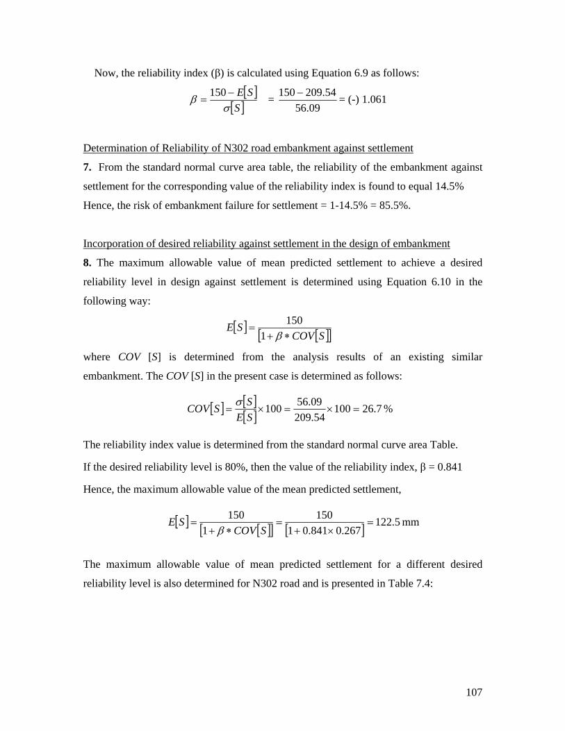
Now, the reliability index (β ca us atio s fo) is lculated ing Equ n 6.9 a llows:
[ ][ ]S
SEσ
β −=
150 = 09.56
54.209150 − = (-) 1.061
Determination of Reliability of N302 road embankment against settlement
7. From the standard normal curve area table, the reliability of the embankment against
settlemen correspon
Hence, the risk of embankme ailure for sett = 1 85
Incorporation of desired relia ity a set n t n of km
t for the ding value of the reliability index is found to equal 14.5%
nt f lement -14.5% = .5%.
bil gainst tlement i he desig emban ent
8. The m e an d nt to achieve a desired
reliability level in design against ent is determi g E n 6
followi
]
aximum allowable valu of me predicte settleme
settlem ned usin quatio .10 in the
ng way:
[ ]] [[ SCOV∗SE
β
where COV [S] is determ ed he s of stin ilar
em [S] in the present case min llow
+1=
150
in from t analysi results an exi g sim
bankment. The COV is deter ed as fo s:
[ ][ ][ ] 7.2600 =10 ×==
EV
54.20909.5610×
SSSCO σ %
ined from th c a T
llowable value of the mean predicted settlement,
e standard normal urve are able. The reliability index value is determ
If the desired reliability level is 80%, then the value of the reliability index, β = 0.841
Hence, the maximum a
[ ] [ ][ ] [ ] 5.122267.0841.0
150150=
×+mm
of mean predicted settlement for a different desired
le 7.4:
11=
∗+=
SCOVSE
β
The maximum allowable value
reliability level is also determined for N302 road and is presented in Tab
107
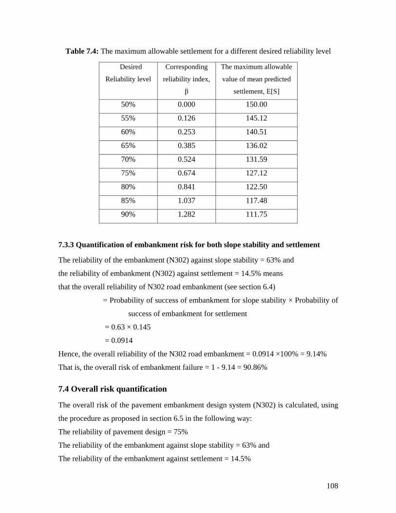
Table 7.4: The maximum allowable settlement for a different desired reliability level
level reliabi dex,
β
value icted
settlement, E[S]
Desired Corresponding The maximum allowable
Reliability lity in of mean pred
50% 0.000 150.00
55% 0.126 145.12
60% 0.253 140.51
65% 0.385 136.02
70% 0.524 131.59
75% 0.674 127.12
80% 0.841 122.50
85% 1.037 117.48
90% 1.282 111.75
ment risk for both slo ty and settlement
road embankment (see section 6.4)
ility of success of embankment for slope st ity × Probability of
success of embankment for settlement
0% = 9.14%
hat is, the overall risk of embankment failure = 1 - 9.14 = 90.86%
7.4 Overall risk quantification
he reliability of pavement design = 75%
he reliability of the embankment against slope stability = 63% and
The reliability of the embankment against settlement = 14.5%
7.3.3 Quantification of embank pe stabili
The reliability of the embankment (N302) against slope stability = 63% and
the reliability of embankment (N302) against settlement = 14.5% means
that the overall reliability of N302
= Probab abil
= 0.63 × 0.145
= 0.0914
Hence, the overall reliability of the N302 road embankment = 0.0914 ×10
T
The overall risk of the pavement embankment design system (N302) is calculated, using
the procedure as proposed in section 6.5 in the following way:
T
T
108

Overall design risk (3 cases)
1.
= [1- (0.75×0.63)] ×100% = 52.75%
2. Risk of pave f e
= [1- (0.75×0.145)] ×100% = 89.13%
3. Risk of pavemen e, failure in ment stability and settlement,
= [1- (0.75×0.63×0.145)] ×100% = 93.15%
7.5 Summary
This chapter provided an integrated e to quantify the overall risk of a pavement
embankment design system for Bangladesh, considering the d laboratory test data
of road N302. The risk in pavement design was found to be 25%, the risk in embankment
design for slope stability was found to and for settle risk was found to be
85.5%. The overall nkment risk was found to be 90.86%. The overall risk of the
pavement-embankment design system considering all possible combinations of failure
was also quantified and for the worst combination was found to be 93.15%. The next
ment
esign data.
Risk of pavement failure and failure in embankment stability,
ment failure and ailure in embankm nt settlement,
t failur embank
xample
field an
be 37% ment the
emba
chapters will consider the development of a process for the quality control of pave
and embankment construction in Bangladesh to reduce the variability in the d
109
Chapter 8 Pavement Construction Quality Control
iability of
entioned in Chapter
cess
lete
cess of a quality control system for Bangladesh. With this in mind, the
pleted quality control procedures in pavement construction are available
arch work is found on the different components
a quality control process, including quality control tests, quality measures, testing
pling and performance relationships. A brief summary of them is
.2.1 Quality control tests
he commonly used quality control measures for pavement construction are density,
moisture content, gradation and layer thickness. These parameters are not consistent with
the performance based construction criterion where evaluating the strength and stiffness
of material is important. More importantly, the stiffness values are used as an input in the
design of pavement systems. A design directly connected with the construction method is
8.1 Introduction
A quality control and assurance system is essential to reduce the var
construction related data. One of the objectives of this research, as m
1, is to develop a quality control and assurance process for the pavement design system of
Bangladesh. The concepts and fundamentals of quality control and assurance pro
were discussed in the literature review chapter. This chapter presents the comp
development pro
review of developed methods and techniques for the quality control of pavement
construction and the comparison of them with respect to the criteria as defined in the
methodology chapter in presented first with a view to identifying a suitable method or
technique for Bangladesh. Next, the logical development leading to the proposed method
is discussed, followed by detailed steps for the proposed procedure. The chapter
concludes by presenting the step-by-step quality control process during construction; this
process was also developed in the present research to make the quality control process
smooth.
8.2 Developed methods
A very few com
in the literature. However, significant rese
of
frequency and sam
presented below.
8
T
110
a prere e for
measuring in situ stiffness is required.
is one of the most critical parameters in pavement design procedures
g the performance of a pavement. Burati and Weed [2006] also suggested
viation jointly to determine specification compliance in the
quality control process of pavement construction. Schmitt et al. [1998] proposed five
pare the mean constructed thickness and the
and McCullough [1991] also suggested using the student’s
quisite for balancing cost effectiveness with quality criteria. Hence, a techniqu
Pavement thickness
but is significantly affected by poor construction practices. Hence, pavement layer
thickness tests are an important part of any quality control process. The direct way to
evaluate pavement layer thickness is by digging a core. But this process is destructive,
time consuming and is not suitable for large-scale evaluation. There are other ways of
evaluating pavement layer thickness, such as using the Dynamic Cone Penetrometer
[Chen et al., 2001] or Ground-Penetrating Radar [Al-Qadi et al., 2003: Saarenketo and
Scullion, 2000].
8.2.2 Quality measures and conformance
Livneh [2002] mentioned that highway agencies in many countries adopt a statistical
approach to evaluate the quality characteristics of pavement construction. Some
advantages of this approach were also reported, such as greater production flexibility, no
need for engineering judgment, decreased disputes over marginal quality work, etc. Weed
[1999] recommended mean and standard deviation as a suitable quality measure in
determinin
using mean and standard de
different measures: average, moving average, average absolute deviation (AAD), range
and quality level analysis for the same purpose. Dobrowolski and Bressette [1998]
reported that the t-test for sample means with a confidence interval of 99 percent should
be used for comparing quality control test results. One-sided and two-sided t-tests were
used by Mladenovic et al. [2003] to com
design values. Torres-Verdin
t-distribution in establishing confidence interval of the mean for quality control
parameters.
111
8.2.3 Performance relationship
A) S shaped performance model
Weed [2006] proposed a multi-characteristic performance relationship for use in quality
control processes. Since, most quality characteristics had points of diminishing returns
(points beyond which little additional performance could gain from still higher levels of
quality), a more appropriate model with an S shape was suggested. An exponential
expression given by the following equation was recommended as a suitable mathematical
form, which could produce an S shape.
CBxAey −= --------------------------------- (8.1)
The equation was recommended when zero took the best possible level of the
roughness or percentage defective, PD). independent variable (x) (say, pavement
However, when zero took the worst possible value (say, pavement thickness or
percentage within limit, PWL) the following equation best represented the model form:
( )CBxeAy −−= 1 ------------------------------- (8.2)
The two equations above were based on a single quality characteristic which was not in
accordance with reality. Weed [2003] extended Equation 8.1 in the following way which
could consider any reasonable number (k) of quality characteristics:
Kko PDBPDBPDBBeEXPLIF ++++= L2211 ------------ (8.3)
where EXPLIF (expected life in years) took the place of dependent variable (y) and PD
took the place of independent variable (x). A performance matrix was suggested for use
in evaluating the co-efficient of the above equation.
B) Simulation method
Patel and Thomson [1998] investigated the effect of variability on system performance by
performing a sensitivity analysis of the quality characteristics with the simulation method
and showed that deviation from the target mean value significantly affected the fatigue
life and there was varied influence on the fatigue life due to deviations from the target
standard deviation.
.2.4 Pay adjustment
Highway agencies throughout the world are now increasingly using adjusted payment
provision for work which fails to meet the desired quality level but is not deficient
8
112
enough to warrant removal and replacement. More recently, many agencies have started
the form of bonuses for work which substantially
ic methods for pay adjustment: a factor (or
r was mentioned a
y
consequently suggested the f
to calculate the future cost:
INF
lated as:
W0 = Cn (1+RINT)n ----------------------
d
]
characteristic by statistical quality
composite pay factor by using weighted individual pay factors.
1] performed a life-cycle cost analysis to develop the link between
onomic gain or loss to the highway agency and suggested the
following equation:
to provide monetary incentives in
exceeds the desired level of quality. Research undertaken by the California Department
of Transportation found that incentives provided by the pay factor encouraged a better
product [Douglas et al., 1999]. However, there are no well-established methods to
determine the magnitude of pay adjustment appropriate for varying levels of as built
quality. Schmitt et al. [1998] investigated the pay adjustment attributes of different
agencies’ specifications and found two bas
multiplier) and a fixed rate. The facto s the more common; it involves a
predetermined pay percentage for measured test results. In contrast, an example of fixed
rate adjustment was given as a $1 per ton pay reduction for a certain level of quality
regardless of bid price. Weed [1998] reviewed earlier work and mentioned that many pay
schedules currently in use may not fully reflect the real costs incurred by highwa
agencies as a result of defective work and ollowing equation
Cn = C0 (1+RINF/100)n ------------------------------- (8.4)
where Cn stands for future cost after n years, C0 for present cost and R for annual
inflation rate (percent). Then the present worth of future cost was calcu
------------- (8.5)
where W0 represents present worth, Cn represents the cost n years in the future an
RINT represents annual interest rate (percent). Dobrowolski and Bressette [1998
suggested determining a pay factor for each quality
analysis and calculating a
Individual and composite pay factors were then suggested for use as a basis for decisions
whether to accept or reject work and also over paying the contractor. Weed [1999]
suggested that pay equations based on the mean and standard deviation derived from the
sample closely correspond the value of the as-built work determined by the life-cycle cost
analysis. Weed [200
quality received and ec
( ) ( )OVLIFEXPLIFDESLIF RRRCPAYADJ −−= 1/ ----------------- (8.6)
113
where PAYADJ = appropriate pay adjustment for pavement or overlay (same unit as C)
C = Present total cost of resurfacing (typical value = $20/yd2 or $23.92/m2)
DESLIF = design life of pavement or overlay (typical 20 years for new pavement,
10 years for overlay)
EXPLIF = expected life of pavement or overlay (independent variable)
OVLIF = expected life of successive overlays (typically 10 years) and
R = (1+INF) / (1+INT) [INF is the long-term annual inflation rate and INT
is the long-term annual interest rate, both in decimal form]
Zaghloul et al. [1998] quantified the payment adjustment factors (PAFs) by performing a
life cycle analysis considering the long-term effects of the initial roughness; they strongly
advised every highway agency to conduct this type of analysis for their local conditions
in order to develop their own PAF.
8.3 Comparison of the de
veloped methods and techniques
A brief
The available methods and techniques are compared with respect to the criteria as
determined in section 3.8 of the methodology chapter with a view to developing a
suitable method of quality control in pavement construction for Bangladesh.
summary of this comparison is presented below.
Quality control tests:
Strength and stiffness tests: The Dynamic Cone Penetrometer (DCP) test is cost effective,
simple to use and easy to maintain [Abu-Farsakh et al., 2005]. There are some verified
correlations in the literature to calculate pavement strength and stiffness from the DCP
test results [Powell et al., 1984; Abu-Farsakh et al. 2005; Chen et al. 2001]. But these
correlations are site specific and no correlation has so far been developed for Bangladesh.
Besides, DCP data collected from road testing in Bangladesh shows unrealistic results, as
discussed in section 4.3.4. Hence, DCP is not suitable for evaluating the strength of
pavement construction in Bangladesh. Falling weight deflectometer (FWD) tests are well
recognized and widely used [Damnjanovic and Zhang, 2006: Noureldin et al., 2003]. The
moduli of pavement layer are easily evaluated using a back calculation process with data
and Roque, 2003]. The moduli thus evaluated are of higher from FWD tests [Mehta
114
quality and more cost effective than lab-measured moduli [Houston et al., 1992; Kim et
d
2006]. Hence FWD could be used in the country’s quality control of pavement
high, the
al., 2007]. This method of calculating pavement strength is consistent with the propose
analytical pavement design system of Bangladesh. In addition, FWD data is clearly
related to pavement performance [Chen and Scullion, 2006; Damnjanovic and Zhang,
construction. However, as the cost of acquisition and maintenance of an FWD is
Benkelman Beam could be used as a much cheaper substitute.
Thickness tests: Although coring is the easiest and most straightforward way of
ent layer thickness, it is destructive and not suitable for evaluating pavem large-scale
data analysis technique used [Al-Qadi et al., 2005].
Besides, GPR is sophisticated and costly, requiring skilled manpower to implement and
. DCP, in contrast, is
l process.
onformance:
evaluations. Ground-Penetrating Radar (GPR) technology has not been used widely for
quality control or pavement assessment purposes, due to reliability issues with the
technique. Various GPR performances were reported by different investigators,
depending on the site surveyed and
thus is not suitable for a developing country such as Bangladesh
simple to understand and easy to implement. Moreover, the changing slope of the depth
versus profile of the accumulated blows of DCP tests corresponds well with the thickness
obtained in the test pits [Chen et al., 2001]. Hence, DCP could be used to assess the
thickness of pavement layers in the quality contro
Quality measures and c
The statistical approach of evaluating the quality characteristics of pavement
construction, as proposed by Livneh [2002], is suitable for Bangladesh since it is well
recognized, widely used and a scientific way of deriving a universal property from a
sample property. Weed [1999] and Burati [2006] suggested mean and standard deviation
is the best measure to determine the population mean of quality characteristics from a
sample mean and hence one which could well be used in the quality control system of
Bangladesh. Dobrowolski and Bressette [1998], Torres-Verdin and McCullough [1991]
and Mladenovic [2003] proposed a t-test to establish a confidence interval of sample
mean which is suitable for any quality control system; this is because a t-test is applicable
for a small number of tests and in the quality control process of construction usually a
small number of tests is performed to make decisions about a large project.
115

Performance relationship:
S shaped performance model: The equation proposed in this method to evaluate
pavement performance for a higher number of quality characteristics involves a number
of co-efficients and it was suggested that these should be used to evaluate by means of a
performance matrix. But a performance matrix is not available in Bangladesh. Besides,
this performance evaluation procedure is not compatible with the proposed design system
of Bangladesh.
Simulation method: The simulation method of evaluating pavement performance by
performing a sensitivity analysis of quality characteristics is not suitable for Bangladesh
since a computer model is required to perform the simulation.
Pay adjustment:
Adjusted payment provision could be used in Bangladesh’s quality control system since
many highway agencies in the world are now increasingly using it and it encourages a
better product, as many researchers have noted. Pay adjustment in the form of a pay
factor would be suitable for Bangladesh, since, as Schmitt et al. report [1998], it is widely
used. The pay adjustment equation proposed by Weed [2001] would be best for
Bangladesh, since it is based on the pavement life cycle cost and compatible with the
proposed design system of Bangladesh.
8.4 Logical development of the proposed method
Performance based quality control
A suitable quality control system for Bangladesh, as defined in the methodology chapter,
should be clearly related to performance; the performance must be consistent, convenient
to measure and quantify and suitable for the country’s pavement design system. The
proposed pavement design system of Bangladesh is an analytical design system where
pavement performance is measured by the critical number of load repetitions that a
pavement can sustain before failure. Considering the criteria of the required quality
control system and the performance measure of analytical pavement design, the critical
number of road repetitions that a pavement can sustain before failure (Ncritical) is selected
as the quality control parameter for the proposed quality control system.
116
To quantify the parameter Ncritical, a pavement structural analysis model based on elastic
d as a suitable method for evaluating pavement layer strength and the
om sampling follows to
each stratum) is identified as a suitable method of sampling for the
discussed in section 8.3. If the population mean
deviates slightly from the design value then provision is also made in the proposed
discussed in section 8.3. The
provided in section 8.5.1.
layered theory is used. The input of this analysis model is determined by testing, which
involves evaluating the strength and thickness of the pavement layer. Some criteria for
suitable quality control tests were defined in the methodology chapter. Investigating the
existing quality control tests with respect to these criteria identifies suitable methods for
Bangladesh, as discussed in section 8.3. The Falling Weight Deflectometer or Benkelman
Beam is identifie
Dynamic Cone Penetrometer is identified as suitable method for evaluating thickness.
Stratified random sampling (where the population is divided into a number of non-
overlapping sub-populations, or strata and then a simple rand
select samples from
quality control of pavement construction since it better represents the actual field than
simple random sampling. In addition, the problem of clustering (clogging of samples
close to each other) in simple random sampling is reduced to some extent in stratified
random sampling. Now, data from the quality tests helps to evaluate the pavement
capacity. To find the population mean of pavement capacity, the mean and standard
deviation of the sample mean is used, as identified in section 8.3. The t test is used to
establish confidence interval of mean as
system to accept the work with adjusted payment, as
detailed procedure for this method is
Step-by-step performance evaluation
In case of performance-based quality control, the road section is tested for acceptance
after the completion of the work. When a completed road section is rejected due to
improper quality it means a loss of resources and time. In most cases, there is a dispute
between the contractor and the road agency which sometimes ends in court. To avoid
these, it will be better to have a system of quality control after the construction of every
layer of pavement, such as a step-by-step method of quality control. Torres-Verdin and
McCullough [1991] proposed a methodology of evaluating pavement performance after
the completion of every layer using the AASHTO structural number parameter
value for the completed layer. However, this method is not compatible with the iii mDa∑
117
proposed analytical pavement design system for Bangladesh. Hence, a methodology for
quality control during construction is proposed in the present research which uses the
critical number of load repetitions that a pavement can sustain before failure (Ncritical) as a
control parameter for pavement performance in order to be compatible with the
analytical design system. The detailed procedure in this method is presented in section
8.5.2
8.5 Proposed Methods
8.5.1 Performance based quality control
In this method the performance of the pavement is considered the main criterion for
acceptance. Pavement performance is measured by evaluating the pavement’s load
carrying capacity. A structural analysis model together with pavement surface deflection
and layer thickness data is used to evaluate pavement capacity in terms of the critical
number of load repetitions before failure (Ncritical). The non-destructive Falling Weight
Deflectometer (FWD) or Benkelman Beam testing is used to measure surface deflection.
A Dynamic Cone Penetration (DCP) test is conducted to evaluate the thickness of the
pavement layers. The evaluated pavement capacity is compared with the required one. If
it is satisfactory then the pavement section being tested is accepted. Since the pavement
performance is selected as the parameter for quality control, the method is named the
‘performance based quality control method of pavement construction’.
flowchart of this method is presented in Figure 8.1 and tA he detailed steps of this
method are described below:
1. The required capacity of the pavement needs to be specified first, so that the evaluated
pavement performance can be judged. A small amount of deviation is acceptable in every
design. Hence, the level of tolerance should also be specified. The road agency usually
specifies the level of tolerance.
2. Then the length of the road to be tested needs to be divided into a number of sections
to carry out the stratified random sampling.
3. Then quality control tests are performed in each section using random sampling which
involves FWD or the Benkelman beam test for surface deflection and DCP or coring for
the layer thickness. The soaked CBR test is also suggested, to better represent the layer
118
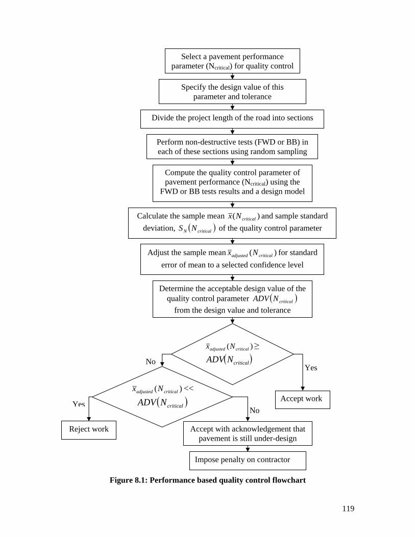
Select a pavement performance parameter (Ncritical) for quality control
Figure 8.1: Performance based quality control flowchart
Accept with acknowledgement that pavement is still under-design
Reject work
Accept work
Perform non-destructive tests (FWD or BB) in each of these sections using random sampling
)(Nx ≥criticaladjusted
( )NADV critical
)( criticaladjusted Nx <<( )NADV critical
Divide the project length of the road into sections
Calculate the sample mean )( criticalNx and sample standard deviation, ( )criticalN NS of the quality control parameter
Specify the design value of this parameter and tolerance
Compute the quality control parameter of pavement performance (Ncritical) using the
FWD or BB tests results and a design model
Adjust the sample mean )( criticaladjusted Nx for standard error of mean to a selected confidence level
Determine the acceptable design value of the quality control parameter ( )criticalNADV
from the design value and tolerance
Yes No
YesNo
Impose penalty on contractor
119
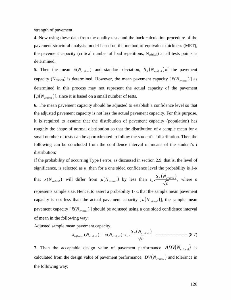
strength of pavement.
4. Now using these data from the rocedure of the
pavement structural analysis model nt thickness (MET),
the pavement capacity (critical number al) at all tests points is
determined.
5. Then the mean
quality tests and the back calculation p
based on the method of equivale
of load repetitions, Ncritic
and standard deviation, ( )of the pavem)( criticalNx criticalN NS ent
capacity (Ncritical) is determin )( criticalNed. However, the mean pavement capacity [ x
ay not represent the actual capacity of the pavem
] as
determined in this process m ent
[ ( )criticalNμ ], since it is based o
6. The mean pavement capaci e level so that
the adjusted pavement capacity is not less the actual pavement capacity. For this purpose,
it is required to assu pavement capacity (population) has
roughly the shape of no
small number of tests can be approximated to follow the student’s t distribution. Then the
following can be concluded from t’s t
distribution:
If the probability of occurring s, the level of
significance, is selected as α, th nce level the obability is 1-α
that
n a small number of tests.
ty should be adjusted to establish a confidenc
me that the distribution of
rmal distribution so that the distribution of a sample mean for a
the confidence interval of means of the studen
Type I error, as discussed in section 2.9, that i
en for a one sided confide pr
( )n
NS will differ from ( )criticalNμ)( criticalNx by less than t criticalN.α , where n
represents sample size. Hence, to as ability 1- α t t the sample mean pavement
capacity is not less than the actua nt capacity [
sert a prob
l paveme
ha
( )criticalNμ ], the sample mean
pavement capacity [ )( criticalNx ] should be adjusted using a one sided confidence interval
of mean in the following way:
Adjusted sample mean pavement capacity,
= )( criticalNx -( )N
)( criticaladjusted Nxnα
of pavement performance A
St criticalN. --------------------- (8.7)
7. Then the acceptable design value is
calculated from the design value of pave
( )criticalNDV
ment performance, ( ) and toleranccriticalNDV e in
the following way:
120
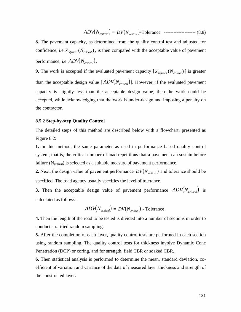
= ( )criticalNADV ( )criticalNDV -Tolerance -------------------- (8.8)
8. The pavement capacity, as determined from the quality control test and adjusted for
confidence, i.e. )( criticaladjusted Nx , is then compared with the acceptable value of pavement
performance, i.e
ed if the [
. ( )criticalNADV .
9. The work is accept evaluated pavement capacity )critical ] is greater
than the acceptable design value [
(adjusted Nx
( )criticalNADV ]. However, if the evaluated pavement
capacity is slightly less than the acceptable design value, then the work could be
accepted, while acknowledging that the work is under-design and imposing a penalty on
ritical number of load repetitions that a pavement can sustain before
the contractor.
8.5.2 Step-by-step Quality Control
The detailed steps of this method are described below with a flowchart, presented as
Figure 8.2:
1. In this method, the same parameter as used in performance based quality control
system, that is, the c
failure (Ncritical) is selected as a suitable measure of pavement performance.
2. Next, the design value of pavement performance ( )criticalNDV and tolerance should be
3. Then the acceptable design v ent perform is
calculated as follows:
( )criticalNADV =
specified. The road agency usually specifies the level of tolerance.
alue of pavem ance ( )criticalNADV
( )criticalNDV - T
4. Then the length of the road to be tested is divided into a number of sections in order to
conduct stratified random sampli
olerance
ng.
ty control tests are performed in each section
using random sampling. The qualit ontrol tes for thickness
Penetration (DCP) or coring, and for strength, field CBR or soaked CBR.
r.
5. After the completion of each layer, quali
y c ts involve Dynamic Cone
6. Then statistical analysis is performed to determine the mean, standard deviation, co-
efficient of variation and variance of the data of measured layer thickness and strength of
the constructed laye
121
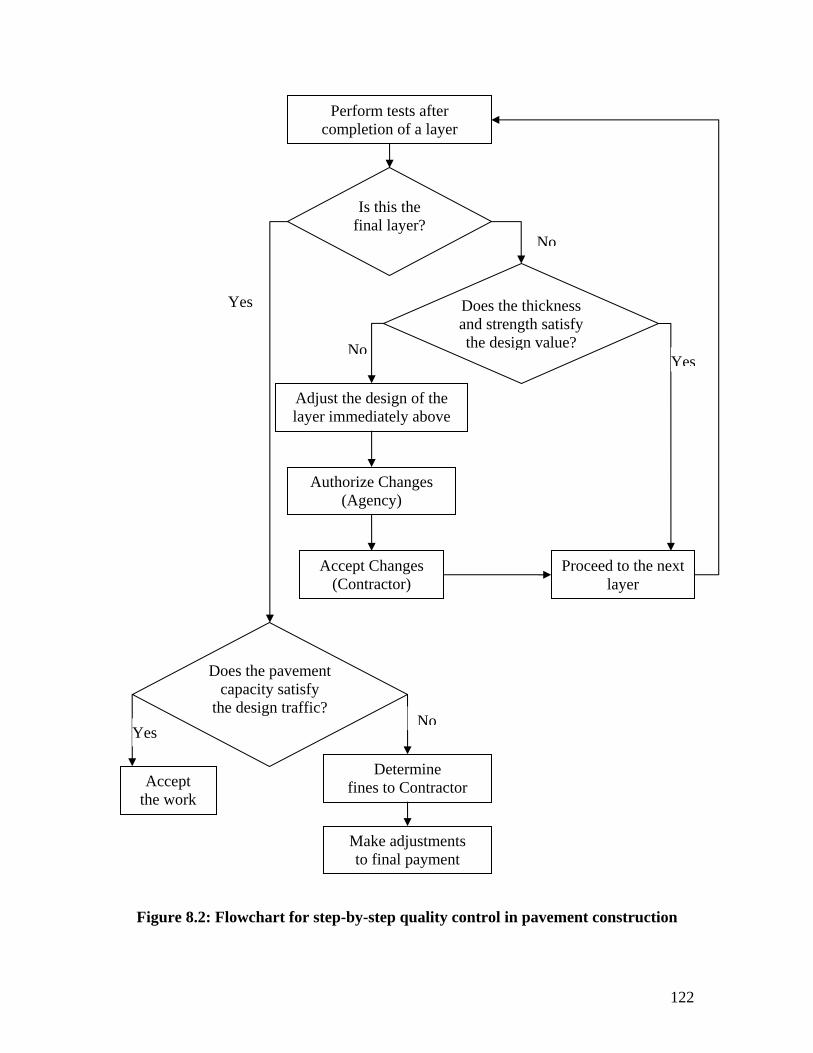
Perfor sts after m tecompletion of a layer
Is this the final layer?
lity control in pavement construction Figure 8.2: Flowchart for step-by-step qua
Accept Changes (Contractor)
Proceed to the next layer
Authorize Changes (Agency)
Accept the work
Make adjustments to final payment
Determine fines to Contractor
Adjust thelayer imme
design of the diately above
Does the thickness and strength satisfy the design value?
Does the pavement capacity satisfy
affic? the design tr
No
Yes
YesNo
NoYes
122
7. The mean thickness and stren mined from a small number of tests.
Hence, the mean value should a confidence level, as discussed in
section 8.5.1. If the level of significance i.e. the probability of occurring Type I error is
selected as α and hence wants to assert a probability 1- α that the adjusted value is not
less than the actual value, then th ean value is adjusted for a one sided
confidence interval of mean in the following way:
gth are usually deter
be adjusted to establish
e sample m
= x - adjustedxn
nt for the selected si
St N.α --------------------------------- (8.9)
where tα represents the normal distribution co-efficie gnificance level
and n represents the sample size.
8. Then the adjusted mean layer thickness and strength are compared with the design
requirements. If satisfacto layer is approved and clearance is
given to start the construction of the next layer.
9. However, if design value is not satisfied then this means that there is a deficiency in
the completed layer. Then th ate above layer should be modified in
such a way that the overall pavement capacity remains the same. The layer thickness or
layer strength of the layer immediately above could be modified in this regard. However,
modifying the design by chang ness only should be
difficult to increase the strength of a layer in the field. The design is modified
considering the requirements of the pavement in the following ways.
10. The pavement capacity (critical number of load repetitions before failure, Ncritical) is
evaluated by t structural analysis with the adjusted data on the mean
layer thicknes e completed layers and the modified design data of the
above unconstructed layer. To this end, a pavement structural analysis model based on
the method of equivalent thickness design is used in this research. However, any other
str odel can be us he evaluated pavement capacity is
compared with the design value [
ry, then the constructed
e design of immedi
ing the layer thick tried first, since it is
pe enrforming pavem
s and strength of th
uctural analysis m ed in this context. T
( )criticalNDV
be
ance [
]. If it is not satisfactory the design of
above unconstructed layer should This process is continued until the
design value of the pavement perform
further modified.
( )criticalN ]DV is satisfied.
11 e
lso the adjusted mean layer thickness and strength are evaluated and compared with the
. The same procedure is followed after the construction of the next layer. In this cas
a
123
design requirements. If a deficiency is found in this layer too then the design of the
unconstructed layer immediately above also needs to be modified. This process is
continued until the construction of the final layer.
12. After final layer is completed, the same procedure as proposed in the performance
based quality control method (section 8.5.1) is followed, to evaluate the quality of the
overall construction. The quality control tests are performed in the different locations and
the adjusted mean pavement capacity [ )( crited s evaluated. ticaladjus Nx ] i
13. The adjusted mean pavement capacity [ )( criticaladjusted Nx ] is then compared with the
ment’s performance [ ( )criticalNADVacceptable design value of the pave ].
14. If it is not satisfied then the work is rejected. However, if the evaluated pavement
capacity [ )( criticaladjusted Nx ] is slightly short of the acceptable design capacity
[ ( )criticalNADV ], then the work is accepted while acknowledging that the pavement is
Benkelman beam
ency and th
in application are
still under-design and a penalty is imposed on the contractor.
8.6 Summary
The chapter presented the complete development procedure of a quality control system
for pavement construction in Bangladesh. In order to do so, the chapter first reviewed the
existing methods and techniques and compared them with respect to some predefined
criteria to identify a suitable technique for Bangladesh. The FWD or
was identified as a suitable test for evaluating pavement strength and the DCP for
evaluating thickness. Stratified random sampling, a t-test, was also identified as suitable
for Bangladesh. Then the detailed procedure was set out of the method which was
developed in this research, with these identified components, taking pavement
performance as the acceptance criterion. In the end the chapter presented the step-by-step
quality control process during construction, which was also developed in this research to
avoid disputes between the road ag e contractor. The next chapter considers
the development of a quality control procedure for embankment construction in
Bangladesh, while examples of the above quality control processes
presented in Chapter 10.
124
Chapter 9 Embankment Construction Quality Control
9.1 Introduction
Embankment construction quality control is an important part of the overall success of
the pavement embankment design system of Bangladesh. This is also an important
objective of this paper. The basic concept, history and statistical measures of quality
control were discussed in the literature rev is chapter begins by reviewing iew chapter. Th
bankment con
ed in methodology chapter with
method is described in detail.
A very few methods are described in the literature for the quality control of embankment
rief summary of them is presented below.
the available methods of quality control in em struction in the literature and
then compares them with respect to some criteria as defin
a view to developing a suitable method for Bangladesh. Then the logical development
leading to the proposed method is presented. Finally the procedure of the proposed
9.2 Developed Methods
construction. A b
9.2.1 Quality control of embankment constructed with soft sedimentary rock
Nakamura et al. [1998] reported that soft rocks tend to exhibit slaking and weathering
when they are excavated from an in-situ high confining pressure state to open-air stress-
free conditions and this weathering weakens them and causes changes in compressibility
in soft sedimentary earth fills which often lead to slope failure and/or extensive
settlement. They proposed the following Talbot equation to express the grain size
distribution of soft rock materials:
( ) %100/ ×= nDdP ------------------------------------- (9.1)
where P is the percentage of materials finer than grain size d, D = maximum grain size: n
= power number. Nakamura et al. [1998] conducted laboratory experiments to investigate
the influence of these factors on soft rock material and proposed a practical and useful
method of quality control for embankments constructed with soft rock materials by using
the degree of compaction (Dn) defined as the ratio of a compacted dry density (ρd) to the
dry density of the intact rock particle (ρt). That is,
125
( ) %100/ ×= tdnD ρρ ------------------------------------ (9.2)
maximum compacted dry density (ρdmax) itself in soft
ed greatly as construction progressed, due to particle breakage and
confining pressure. Then the test results were redrawn for
a relationship between n and Pv for different representative combinations of R and Dn (see
a et al. [1998] used the second graph to calculate the
determined values of n and
Dn.
construction. Moisture content, lift thickness, density,
cted as the key crit
They reported that the value of
rock material chang
was not a good reference for comparison. For this reason compacted dry density (ρd) was
used in the above equation instead of the generally used ρdmax. They plotted their test
results summary in the following way: first, the strength reduction due to weathering
(expressed as the strength ratio of the deviator stresses after weathering process to that
before them, R%) was plotted against parameter n for different combinations of degrees
of compaction (Dn) and confining pressure (Pv) value (see Appendix F-1a). It was
reported in interpreting this graph that the strength reduction could be restrained by
increasing the finer content (decreasing n value), by compacting in higher density and by
increasing overburden vertical
Appendix F-1b). Nakamur
equivalent thickness of the overburden soil layer necessary to avoid strength reduction
(R=100%) by reading the corresponding value of Pv for the
9.2.2 End-result based embankment construction quality control procedure
The Iowa Department of Transportation (Iowa DOT) proposed an end-result based
procedure for embankment construction quality control and assurance, using a Dynamic
Cone Penetrometer (DCP) and moisture and density tests [Larsen et al. 2007]. Their
embankment quality control policy had three main components: personnel training,
quality control testing and test strip
stability and uniformity were sele eria to evaluate embankment quality.
Control limits were set for moisture content at +/-2.0% of standard proctor optimum
moisture content and for density not less than 95% of standard proctor maximum dry
density. To check the embankment construction quality with regard to stability and
uniformity, a new parameter termed the average DCP index and variations in the DCP
index were used. The weighted average method was used to calculate the average DCP
index yielding the following equation:
126
2n d ---------------------------- (9.3) Average DCP Index 1=iH
where n represents the total number of blows, di represents penetration distance for the ith
blow and H represents the depth of the desired test layer. The typical value of the DCP
index was suggested for stiff soils 25mm/blow and for soft soils 100mm/blow.
The variation in the DCP index was calculated using the following equation:
Variation in DCP Index =
1 ∑= i
12 1 .1−= −∑ − i
n
i ii dddH
-------------------- (9.4)
where n represents the total number of blows, di penetration distance for the ith blow and
H depth of the desired test length. It was reported that, for well-compacted fill, a value of
variation in the DCP index of around 5-20mm/blow is reasonable, although ideally it
should be zero. It was suggested for constructing a test strip to establish proper rolling
patterns, the number of roller passes and lift thickness (thickness of a stage of
construction in a vertical direction) required to attain acceptable compaction. Random
testing was suggested for moisture content, density, DCP index and variation in DCP
index. Construction of a new test section was recommended if the type of soil or
compaction methods/equipment needed to change.
9.2.3 AASHTO [1996] Guideline
ines for The AASHTO [1996] quality assurance guide specification provided some guidel
quality control and acceptance decisions in embankment construction. The guide
suggested that the contractor is responsible for quality control and should submit a
quality control plan for approval before work started. It was also suggested that all
required field inspections, sampling and testing to determine the various properties as
specified in the specification should be directed by the certified technician. Quality
control tests were suggested to be statistically random and testing should be in
accordance with the specification. The acceptance limits which were suggested for the
evaluation of earthwork in an embankment are presented in Table 9.1.
127
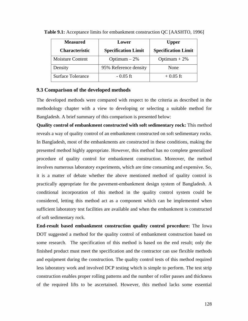
Table 9.1: A ent constructcceptance limits for embankm ion QC [AASHTO, 1996]
Measured
Characteristic
Lower
Specification Limit
Upper
Specification Limit
Moisture Content Optimum – 2% Optimum + 2%
Density 95% Reference density None
Surface Tolerance - 0.05 ft + 0.05 ft
9.3 Comparison of the developed methods
The developed methods were compared with respect to the criteria as described in the
methodology chapter with a view to developing or selecting a suitable method for
Bangladesh. A brief summary of this comparison is presented below:
Quality control of embankment constructed with soft sedimentary rock: This method
reveals a way of quality control of an embankment constructed on soft sedimentary rocks.
In Bangladesh, most of the embankments are constructed in these conditions, making the
presented method highly appropriate. However, this method has no complete generalized
procedure of quality control for embankment construction. Moreover, the method
involves numerous laboratory experiments, which are time consuming and expensive. So,
the above mentioned method of quality control is
e flexible methods
nd equipment during the construction. The quality control tests of this method required
ss laboratory work and involved DCP testing which is simple to perform. The test strip
onstruction enables proper rolling patterns and the number of roller passes and thickness
f the required lifts to be ascertained. However, this method lacks some essential
it is a matter of debate whether
practically appropriate for the pavement-embankment design system of Bangladesh. A
conditional incorporation of this method in the quality control system could be
considered, letting this method act as a component which can be implemented when
sufficient laboratory test facilities are available and when the embankment is constructed
of soft sedimentary rock.
End-result based embankment construction quality control procedure: The Iowa
DOT suggested a method for the quality control of embankment construction based on
some research. The specification of this method is based on the end result; only the
finished product must meet the specification and the contractor can us
a
le
c
o
128
com ity
measures, esta f a confidence test results and a decision procedure
regarding s work. ion for the
quality c ents cons sedimen
AASHTO [1996] Guidelines: guide specification gives some
suggestions and guidelines for quality control in embankment construction. However, the
specification guide does not provide any quality control method or procedure for this
guide could be used at times in the
y and uniformity of embankments. The Iowa
ponents of a complete quality control procedure, such as the appropriate qual
blishment o
lightly deficient
interval of
Moreover, no provis exists in this method
ontrol of embankm tructed with soft tary rock.
This quality assurance
purpose. Nevertheless, the suggestions of this
proposed quality control system for embankment construction in Bangladesh.
9.4 Logical development of the proposed method
According to the criteria defined in the methodology chapter, this method of quality
control must be in accordance with the embankment design system, convenient to
measure and quantify and easy to understand and implement. The existing literature with
respect to these criteria provides no method perfectly suitable for Bangladesh, as
discussed in section 9.3. However, some elements mentioned in the literature were
identified as suitable (see section 9.3) and used in developing the proposed quality
control system of Bangladesh. Nakamura et al. [1998] proposed a quality control
procedure which is used as a component of the proposed quality control process and it is
suggested that these should be implement when the embankment is constructed with soft
sedimentary rock and sufficient laboratory test facilities exist. The Iowa DOT proposed
an average DCP index and variation in DCP index, which are also used in the proposed
procedure as a suitable measure of stabilit
DOT’s recommended provision of test strip construction is also incorporated in the
proposed procedure for Bangladesh. The AASHTO guide specifications as presented in
Table 9.1 are suggested as useful in determining the quality of conformance for
acceptance decisions. Stratified random sampling identified as suitable for highway
construction (see section 8.3) is also used in tests sampling for embankment quality
control. To find the population mean of quality characteristics, the mean and standard
deviation of the sample mean are used since it was identified as a suitable quality
measure in section 8.3. The t- test is used to establish the confidence interval of the mean.
129
Provision is also made for adjusting payment in the proposed procedure for reasonable
deviation from the acceptance specification. A detailed description of the proposed
method is presented in section 9.5.
9.5 Detailed description of the proposed method
The detailed description of the proposed method is given below with a flowchart, as
presented in Figure 9.1.
Step 1: First it must be ascertained whether sufficient laboratory facilities exist, since the
quality control of embankments constructed with soft sedimentary rock particle requires
significant laboratory experiment. Sufficient laboratory facilities are usually provided in
to step-4. every large project. If they are, go to step 2; otherwise, go
Step 2: The next step is to determine the characteristics of the fill material. If the
embankment is to be constructed with soft sedimentary rock materials then a
supplementary quality control programme should be incorporated in the overall quality
control method of embankment construction. If embankment construction material is soft
sedimentary rock, go to step 3; if not, go to step 4.
Step 3: The steps of the supplementary quality control programme are set out below:
i) First the degree of compaction (Dn), defined as the ratio of a compacted dry
density (ρd) to the dry density of the intact rock particle (ρt), should be
determined. Here compacted dry density is used instead of maximum compacted
dry density, since for soft sedimentary rock the value of maximum compacted dry
density changes as the construction proceeds, as mentioned above.
ii) Then laboratory tests must be conducted to determine the relation between initial
gradations, field density and confining pressure with strength reduction. To this
end, a cylindrical specimen of rock material is taken from the field and passed
through five cycles of a wetting and drying weathering process under a specified
constant vertical pressure which is then loaded vertically in a triaxial cell with a
lateral confining pressure of 100~300kpa, as recommended by Nakamura et al
[1998], to obtain the after weathering shear strength. The tests are to be performed
for different test conditions (i.e., for various vertical loads, n-values and degrees
of compaction). Then the tests results must be plotted as in Appendix F-1a with
130
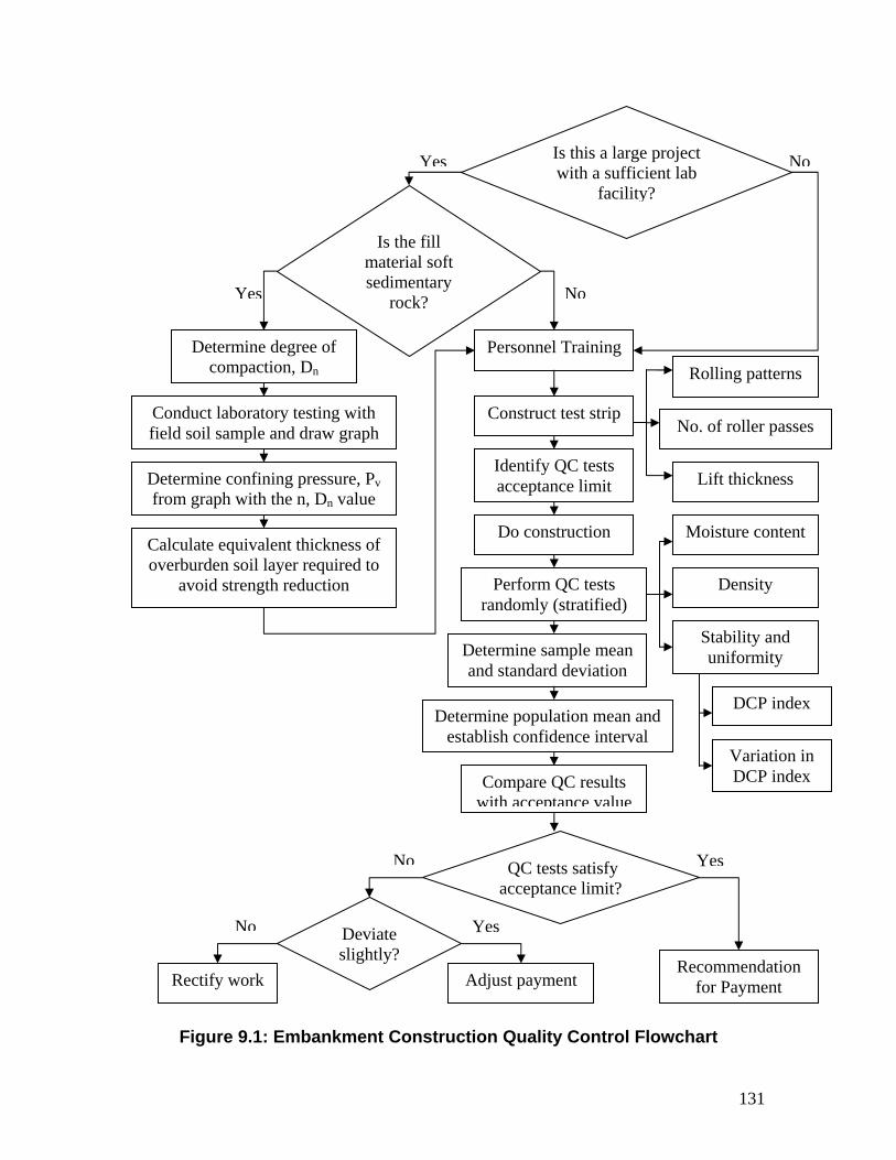
Is this a large project
Figure 9.1: Embankment Construction Quality Control Flowchart
with a sufficient lab facility?
Personnel Training
Calculate equivalent thickness of overburden soil layer required to
avoid strength reduction
Determine confining pressure, Pv from graph with the n, Dn value
Compare QC results with acceptance value
Construct test strip
Perform QC tests randomly (stratified)
Determine degree of compaction, Dn
Is the fill material soft sedimentary
rock?
Yes No
Yes No
Stability anuniformity
d
Moisture content
DCP index
Variation in ndex DCP i
Density
Lift thickness
No. of roller passes
Rolling patterns
QC tests satisfy acceptance limit?
Recommendafor Paymen
Y
tion t
esNo
Conduct laboratory testing with field soil sample and draw graph
Identify QC tests acceptance limit
Do construction
Determine sample mean and standard deviation
Determine population mean and establish confidence interval
Deviate slightly?
Adjust payment Rectify work
YesNo
131
the strength ratio (the strength after weathering process to that before) on
ordinates for every combination o testing condit
iii) Then the tests results should be redrawn as in Appendix F-1b to establish the
relationship between the n-value and confining pressure for different
representative values of the strength ratio R (80%, 90% and 100%).
iv) Then t lue of the con e, pv, necessary to avoid strength reduction
for specified conditions of field grain gradation (n) and degree of compaction (Dn)
s rom the graph.
v) Then the thickness of the surface soil layer which should be overlaid
to be determi
the overburden load is limited then a sligh
provided mater n is kept
n at 85-90%.
Step-4: oce t constru
tra supervision. Personnel training is the most important
steps i ess since all field nd testing
carried out by these personnel.
Step-5: Then a test strip is constructed to d lling pa
required number of roller passes and the requi ieving acceptable
compaction.
Step-6: Then the acceptance limit of quali he AAS
quality assurance guide specification [1996] sug ceptance limi
moisture content and density is recommended for this purpose. For DCP index typical
value of 25mm/blow for stiff soil and 100mm/blow for soft soils could be used for the
acceptance decision. For variation in DCP index, th aken
as reasonably accurate for an acceptance decision.
Step-7: The quality control performe mpletion of construction of
the specified sections using random sampling. These tests inclu
content, density, stability and uniformity. The ex and variatio
index are evaluated to test the stability and uniformity of the constructed embankment.
f the ions.
he va fining pressur
hould be determined f
to achieve
ned. the confining pressure needs
vi) If sufficient soil material for t strength
reduction could be allowed,
and the degree of compactio
ials after excavatio at n ≤ 0.6
The next step in the quality control pr
ining of personnel involved in the
n the quality control proc
ss of embankmen ction is the
inspection, sampling a will be
etermine the required ro
red lift thickness for ach
ttern, the
ty control tests is identified. T HTO
t for gested (Table 9.1) ac
e value 5-20mm/blow could be t
tests are
stratified
d after the co
de moisture
n in DCP average DCP ind
132
Step-8: Then the mean and standard deviation of quality control tests results are
determ
process embankment since it is
not less than
ined. However, the mean value of the quality characteristics as determined in this
does not represent the actual quality characteristics of the
based on a small number of tests.
Step-9: Hence, the mean value of the quality characteristics is adjusted to establish a
confidence level so that the adjusted value of the quality characteristics is
the actual value. This is done in the following ways for a one sided confidence interval of
mean (as discussed in section 8.5.1).
Adjusted sample mean pavement capacity,
S )( sticscharacterixadjusted = )(charactx sticseri -
nt N.α
For a two sided confidence interval (moisture content), the value of confidence limits are
determined by adjusting the sample mean in the following way:
)( sticscharacterixadjusted = x - n
t N.2/α and S
)( sticscharacterixadjusted = x + n
t N.2/α
Step-10: The adjusted mean values of quality characteristics are then compared with
acceptance limit.
Step-11: If the quality control t
S
ests results (adjusted mean) satisfy the acceptance limit
work could be accepted while adjusting the payment of contractor.
, the comprehensive quality control
g
then the work is recommended for payment; otherwise the work is rejected and
rectification suggested. However, if the tests results deviate slightly from the acceptance
limit then the
9.6 Summary
The chapter briefly reviewed first the different embankment quality control methods and
guidelines available in the literature. Then it critically compared the existing methods to
select or develop a suitable method for Bangladesh. Thereafter the logical development
of the proposed method was discussed. Finally
procedure which is proposed for embankment construction in Bangladesh was presented
in detail with a flowchart. In the proposed procedure, provision is made for the quality
control of embankment constructed of soft sedimentary rock material. Provision is also
made for personnel training and test strip construction. The typical value and limitin
133

value of quality control tests results are also specified in the proposed procedure. The
adjusted payment provision is made in the proposed procedure to ease the acceptance
decision when the work slightly deviates from specification. The next chapter will
provide an example of applying the proposed quality control procedure of pavement
construction using field data from Bangladesh.
134
Chapter 10 An example applying the quality control process
10.1 Introduction
This chapter considers an example of the proposed quality control procedure in practice,
sing the field testing data from one of the national highways (N302) of Bangladesh. To
egin with, the performance based quality control process is explained with field data and
ext an example of step-by-step quality control process is presented.
0.2 Application example of the proposed method with field data
ethod is illustrated with the field testing data collected from road N302.
ent capacity is evaluated with field testing data. In the illustrative examples a
ent structural analysis model based on the method of equivalent thickness design is
ent performance. The field testing data of the same road is
trate the step-by-step quality control procedure.
0.2.1 Performance based quality control example
performance based quality control, pavement performance is measured after
onstruction is completed. The detailed steps of this method with field data are described
elow:
. The design value of pavement capacity, that is, the critical numbers of load repetitions
efore failure, is selected as 0.25 million standard axles and tolerance is set as 10% of
esign value.
. Then the project length of the road is divided into sections. Random testing data of
nly one section (the 7th km.) of road N302 is considered in this example.
. Six series of quality control tests were performed in the selected section. As an FWD is
ot available in Bangladesh, the Benkelman beam was used to measure the surface
eflection. Pavement granular layer (base and sub-base) thickness is calculated from DCP
sts data. Coring was done to measure the surface layer thickness. Pavement granular
yer strength (CBR) and stiffness (resilient modulus, Mr) values are estimated from the
DCP test data. Empirical correlations from the literature are used in this regard [Harison,
1987: Rada and Witczak, 1981]. The subgrade resilient moduli are determined from the
u
b
n
1
The proposed m
The pavem
pavem
considered to evaluate pavem
also used to illus
1
In
c
b
1
b
d
2
o
3
n
d
te
la
135
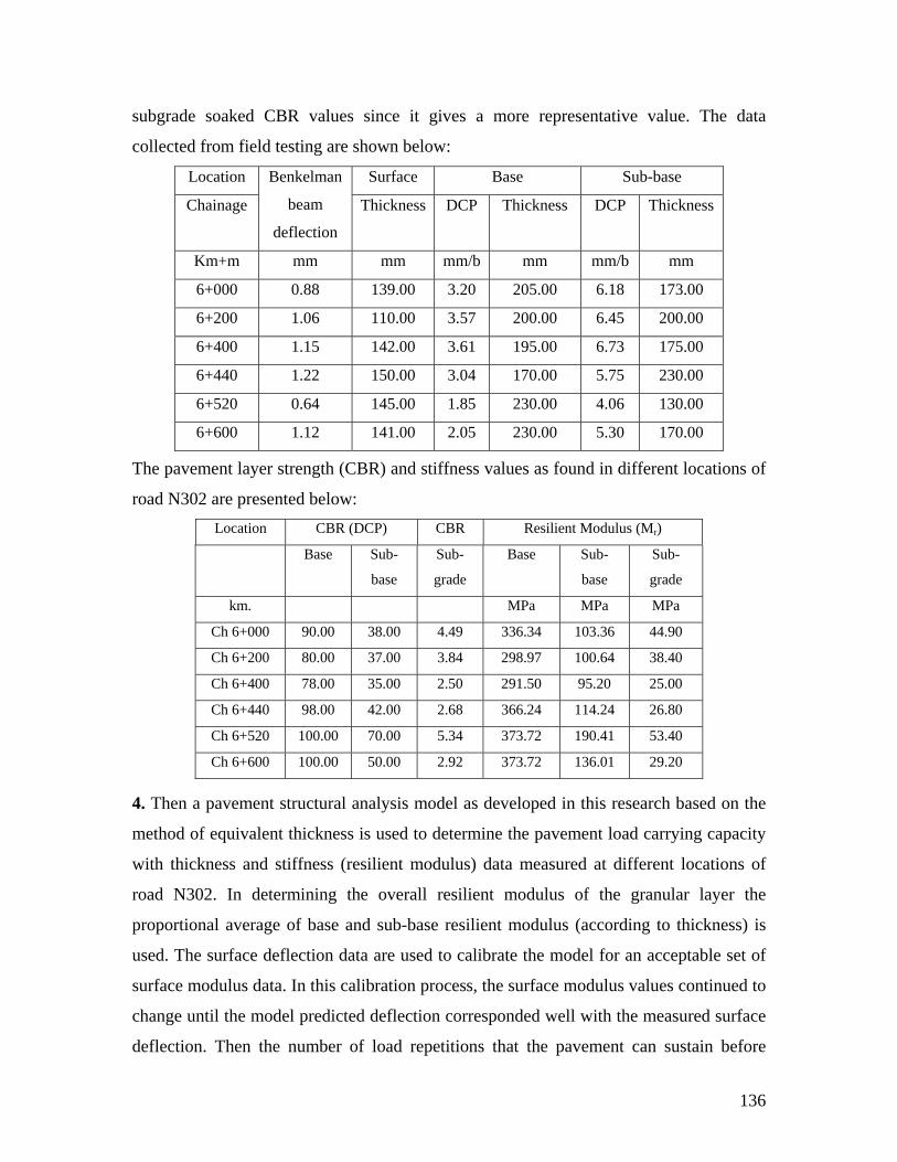
s
collected from field testing are shown below:
Base Sub-base
ubgrade soaked CBR values since it gives a more representative value. The data
Location Surface
Chainage
Benkelman
beam Thickness DCP Thickness DCP Thickness
deflection
Km+m mm mm mm/b mm mm/b mm
6+000 0.88 139.00 3.20 205.00 6.18 173.00
6+200 1.06 110.00 3.57 200.00 6.45 200.00
6+400 1.15 142.00 3.61 195.00 6.73 175.00
6+440 1.22 150.00 3.04 170.00 5.75 230.00
6+520 0.64 145.00 1.85 230.00 4.06 130.00
6+600 1.12 141.00 2.05 230.00 5.30 170.00
The pavement layer strength (CBR) and stiffness values as found in different locations of
road N302 are presented below: Location CBR (DCP) CBR Resilient Modulus (Mr)
Base Sub- Sub- Base Sub-
base
Sub-
grade base grade
km. MPa MPa MPa
Ch 6+000 90.00 38.00 4.49 336.34 103.36 44.90
Ch 6+200 80.00 37.00 3.84 298.97 100.64 38.40
Ch 6+400 78.00 35.00 2.50 291.50 95.20 25.00
Ch 6+440 98.00 42.00 2.68 366.24 114.24 26.80
Ch 6+520 100.00 70.00 5.34 373.72 190.41 53.40
Ch 6+600 100.00 50.00 2.92 373.72 136.01 29.20 4. Then a pavement structural analysis model as developed in this research based on the
method of equivalent thickness is used to determine the pavement load carrying capacity
with thickness and stiffness (resilient modulus) data measured at different locations of
road N302. In determining the overall resilient modulus of the granular layer the
proportional average of base and sub-base resilient modulus (according to thickness) is
used. The surface deflection data are used to calibrate the model for an acceptable set of
surface modulus data. In this calibration process, the surface modulus values continued to
change until the model predicted deflection corresponded well with the measured surface
deflection. Then the number of load repetitions that the pavement can sustain before
136
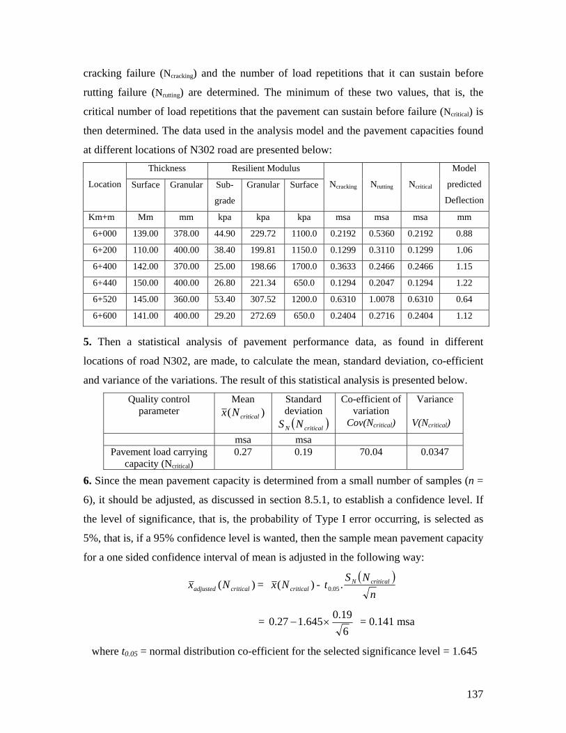
cracking failure (Ncracking) and the number of load repetitions that it can sustain before
rutting failure (Nrutting) are determined. The minimum of these two values, that is, the
critical f on e paveme sustain before failure (Ncritical) is
then de The sed ly d pa
at different location road are presented below: ickness Resilient Mo
number o load repetiti
data u
s of N302
s that th nt can
termined. in the ana sis mo el and the vement capacities found
Th dulus
Location e Gra Sub-
grad
lar ace N N
Model
redicted
eflection
Surfac nular Granu
e
Surf Ncracking rutting critical p
D
Km+m m kpa a mm Mm m kpa kp msa msa msa
6+000 37 44.9 72 0.0 0. 0. 0.88 139.00 8.00 0 229. 110 0.2192 5360 2192
6+200 40 38.4 81 0.0 0. 0. 1.06 110.00 0.00 0 199. 115 0.1299 3110 1299
6+400 37 25.0 66 0.0 0. 0. 1.15 142.00 0.00 0 198. 170 0.3633 2466 2466
6+440 150.00 400.00 26.80 221.34 650.0 0.1294 0.2047 0.1294 1.22
6+520 145.00 360.00 53.40 307.52 1200.0 0.6310 1.0078 0.6310 0.64
6+600 141.00 400.00 29.20 272.69 650.0 0.2404 0.2716 0.2404 1.12 5. Then a statistical analysis of pavem
locations of road N302, are made alc he mean, standard deviation, co-efficient
and variance of the variations. The result of this statistical analysis is pres below.
Q tror
ent performance data, as found in different
, to c ulate t
ented
uality con l paramete
Mean )( criticalNx
ndaiatio
Sta rd dev n ( )critiNS calN
Co-e of va
Cov(N )
ance
tical)
fficient riation
critical
Vari V(Ncri
msa msa Pave arr
ca.19 47 ment load c ying
pacity (Ncritical) 0.27 0 70.04 0.03
6. Since th ve apa de ned sm ber of samples (n = e mean pa ment c city is termi from a all num
6), it should be adjusted, as discussed in section 8.5.1, to establish a confidence level. If
the level of significance, that is, the probability of Type I error occurring, is selected as
5%, that is, if a 95% confidence level is wanted, then the sample mean pavement capacity
for a one sided confidence interval of mean is adjusted in the following way:
)( criticaladjusted Nx = )( criticalNx - ( )
nNS
t criticalN.05.0
= 619.0645.127.0 ×− = 0.141 msa
where t0.05 = normal distribution co-efficient for the selected significance level = 1.645
137
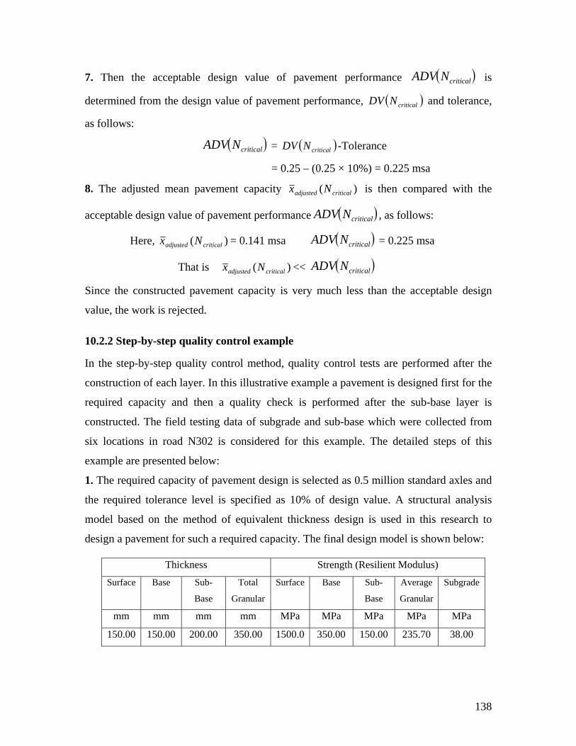
7. Then the acceptable design value of pavement performance ( )criticalNADV is
determined from the design value of pavement performance, ( )criticalNDV and tolerance,
as follows:
( )criticalNADV = ( )criticalNDV -Tolerance
= 0.25 – (0.25 × 10%) = 0.225 msa
8 em c. The adjusted mean pav ent apacity )critical i(adjusted Nx s o
acceptable d val pav nt performan
then c mpared with the
esign ue of eme ce ( )icalNADV ,crit as follo
H
ws:
ere, ) = 0( criticalNadjusted .1 x 41 msa ( )criticalV NAD = 0.225
msa
That is )( criticalNadjustx ed << ( )lV criticaNAD
Si e ct m p v uch less than the acceptable n
value, the work is re
e
required en a q chec u er is
constructed. The field testing data of subgra b-ba er llect from
six locations in road N302 is considered for this example. The detailed steps of this
example are presented below:
nce th constru ed pave ent ca acity is ery m desig
jected.
10.2.2 Step-by-step quality control example
In the step-by-step quality control method, quality control tests are performed after the
construction of each layer. In this illustrative example a pavement is designed first for th
capacity and th uality k is perform
de and su
ed after the s
e which w
b-base lay
s e co ed
1. The required capacity of pavement design is selected as 0.5 million standard axles and
the required tolerance level is specified as 10% of design value. A structural analysis
model based on the method of equivalent thickness design is used in this research to
design a pavement for such a required capacity. The final design model is shown below:
Thickness Strength (Resilient Modulus)
Surface Base Sub-
Base
Total
Granula
Surface Base Sub-
Base
Average
Granular
Subgrade
r
mm mm mm mm MPa MPa MPa MPa MPa
150.00 150.00 200.00 350.00 150.00 235.70 1500.0 350.00 38.00
138
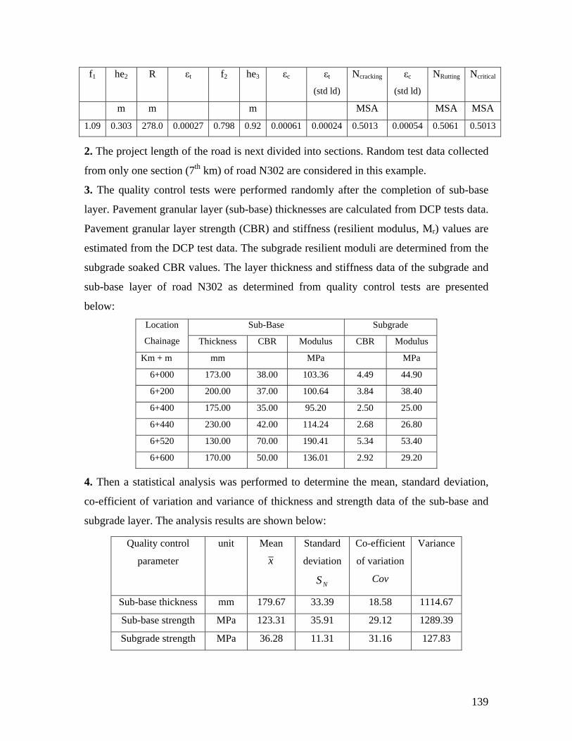
f1 he2 R εt f2 he3 εc εt (std ld)
Ncracking ε
criticalc (std ld)
NRutting N
m m m MSA MSA MSA
1.09 0.303 278.0 0.00027 0.798 0.92 0.00061 0.00024 0.5013 0.00054 0.5061 0.5013
e road is next ided into sections. Random test data collected
randomly afte
ses are calcula tests data.
Pavement granular layer strength (CBR) and stiffness (resilient modulus, M ) values are
oduli are
The layer thick s and stiffness ata of the subgrade and
Sub-Base Subgrade
2. The project length of th div
from only one section (7th km) of road N302 are considered in this example.
3. The quality control tests were performed r the completion of sub-base
layer. Pavement granular layer (sub-base) thicknes ted from DCP
r
estimated from the DCP test data. The subgrade resilient m determined from the
subgrade soaked CBR values. nes d
sub-base layer of road N302 as determined from quality control tests are presented
below: Location
Modulus CBR Modulus Chainage Thickness CBR
Km + m mm MPa MPa
6+000 173.00 38.00 103.36 4.49 44.90
6+200 200.00 37.00 100.64 3.84 38.40
6+400 175.00 35.00 95.20 2.50 25.00
6+440 230.00 42.00 114.24 2.68 26.80
6+520 130.00 70.00 190.41 5.34 53.40
6+600 170.00 50.00 136.01 2.92 29.20
4. Then a statistical analysis was performed to determine the mean, standard deviation,
co-efficient of variation and variance of thickness and strength data of the sub-base and
subgrade layer. The analysis results are shown below:
Quality control unit Mean Standard Co-efficient Variance
x de
v
viation of variation
N
parameter
CoS
Sub-base thickness mm 33.39 179.67 18.58 1114.67
Sub-base strength MPa 123.31 35.91 29.12 1289.39
Subgrade strength MPa 36.28 11.3 83 1 31.16 127.
139
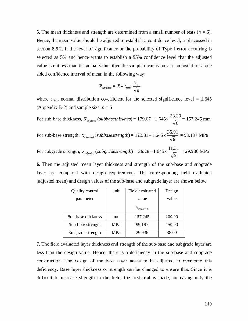
5 he n t knes d str th dete ined f a umb =
Hence, the mean value should be adjusted to establish a confidence level, as discussed in
ection .2. the le el of s nifi ce or I rror in
t d w t a 9 f le u
. T mea hic s an eng are rm rom small n er of tests (n 6).
s 8.5 If v ig can the probability of Type e occurr g is
selec ed as 5% an hence ants o est blish a 5% con idence vel that the adj sted
value is not less than the actual value, then the sample mean values are adjusted for a one
sided confidence interval of mean in the following way:
x adjustedx = - n
St N.05.0
where t0.05, normal distribution co-efficient for the selected significance level = 1.645
(Appendix B-2) and sample size, n = 6
For sub-base thickness, )( cknessubbasethixadjusted = 639.33645.167.179 ×− = 157.245 mm
For sub-base strength, )( engthsubbasestrxadjusted = 691.35645.131.123 ×− = 99.197 MPa
For subgrade strength, )( rengthsubgradestxadjusted = 631.111 ×−
6. Then the adjusted mean layer thickness and strength of the sub-base and subgrade
layer are com ments. The corresponding field evaluated
(adjusted mean desig of -ba ubgr ayer own below.
lity c
arame
F luate
e
645.28.36 = 29.936 MPa
pared with design require
) and n values the sub se and s ade l are sh
Qua ontrol
p ter
unit ield eva d
valu
Desi
valu
gn
e
adjustedx
Sub-base thickness mm 157.245 200.00
Sub-base strength MPa 99.197 150.00
Subgrade strength MPa 29.936 38.00
7. The field layer thickness and reng u u grade layer are
less than the design value. Hence, there is a deficiency in the sub-base and subgrade
constru of ba e be a to e this
deficiency. Base layer thickness or strength can to ensure this. Since it is
difficult e f f al is m incre nly the
evaluated st th of the s b-base and s b
ction. The design the se layer n eds to djusted overcom
be changed
to increase strength in th ield, the irst tri ade, asing o
140
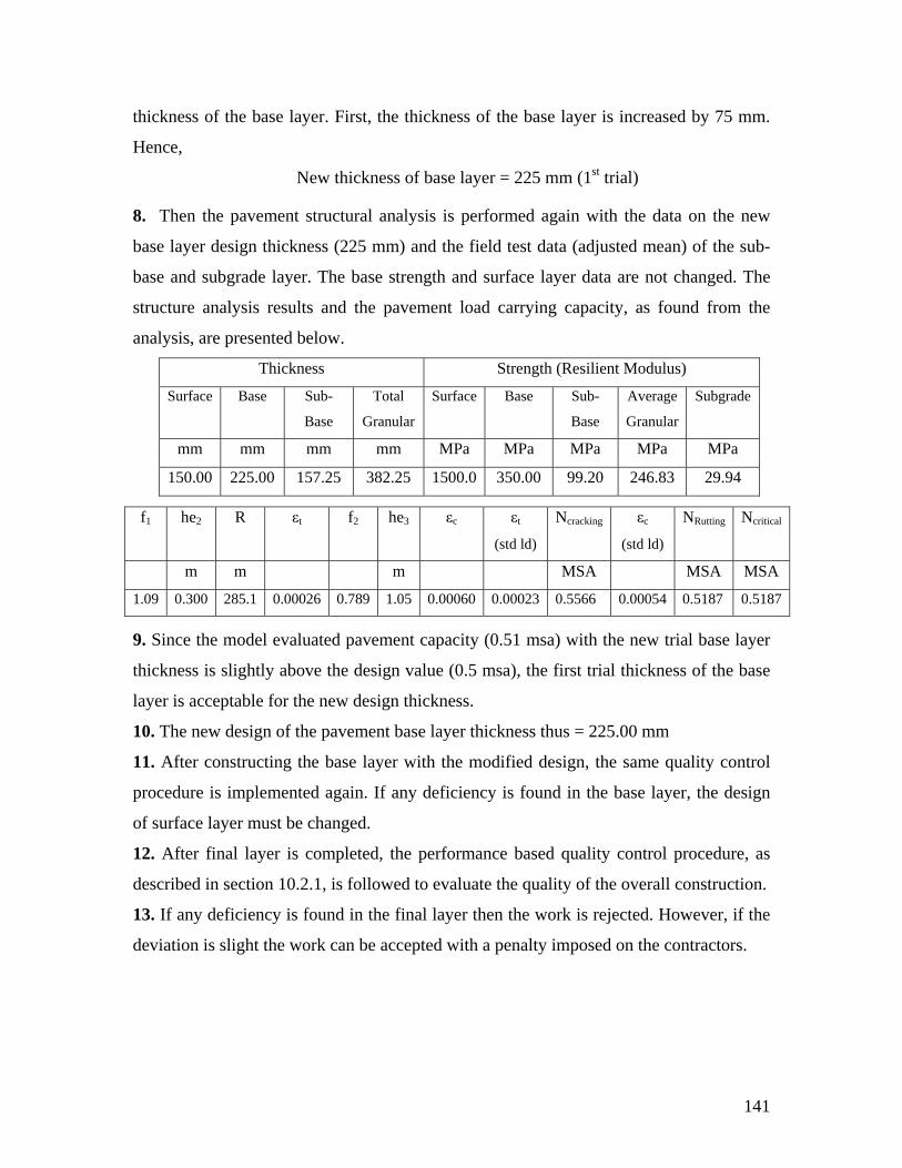
thickness of the base layer. First, the thickness of the base layer is increased by 75 mm.
Hence,
New thickness of base layer = 225 mm (1st trial)
8. Then the pavement structural analysis is performed again with the data on the new
base layer design thickness (225 mm) and the field test data (adjusted mean) of the sub-
base and subgrade layer. The base strength and surface layer data are not changed. The
e pav e load ca ying capacity, as found from the
analysis, are presented below.
structure analysis results and th em nt rr
Thickness Strength (Resilient Modulus)
Surface Base Sub- Total
Base lar Granular
Surface Base Sub-
Base
Average
Granu
Subgrade
mm mm mm mm MPa MPa MPa MPa MPa
150.00 225.00 83 29.94 157.25 382.25 1500.0 350.00 99.20 246.
f1 he2 R εt f2 he3 εc εt td ld)
Ncracking εc (std l
NRutting Ncritical
(s d)
m m m MSA MSA MSA
1.09 0.300 285.1 0.00026 0.789 1.05 0.00060 0.00023 0.5566 0.00054 0.5187 0.5187
9. Since the model evaluated pavement capacity (0.51 msa) with the new trial base layer
thickness is slightly above the design value (0.5 msa), the first trial thickness of the base
layer is acceptabl sign thicknes
10. The new design of the pavement base layer thickness thus = 225.00 mm
11. After constructing the base layer with the modified design, the same quality control
procedure is im f an iciency is found in the base layer, the design
of surface layer
12. After final , th ormance based quality control procedure, as
e for the new de s.
plemented again. I y def
must be changed.
layer is completed e perf
described in section 10.2.1, is followed to evaluate the quality of the overall construction.
13. If any deficiency is found in the final layer then the work is rejected. However, if the
deviation is slight the work can be accepted with a penalty imposed on the contractors.
141

10.3 Summary
The chapter presented an example of applying the quality control process of Bangladesh
onsidered in this
for pavement construction. The field testing data of road N302 was c
regard. Both the performance based quality control process and the step-by-step quality
control process were explained with data from the field. The next chapter will consider
the overall discussion of this research, following which Chapter 12 will conclude this
study.
142

Chapter 11 Discussion
ate a quality control system in this system, with a view to reducing the variability
ent and embankment design parameters were
llected for these parameters from field and laboratory
ferent locations on some of the country’s representative roads. The data were
s developed for Bangladesh to quantify the
ent and embankment design associated with variability in data. Since the
ent and embankment will act as an integral system, an overall risk quantification
ethodology was also developed. Then the overall risk of one of the roads of
was quantified according to the proposed method. A methodology for
ent and embankment construction quality control was also developed in this
ethods were presented to some representative engineers of
ent of Bangladesh and their opinion was studied, since
ately use these developed methods. Some
endations were also identified which would reduce the risk in design and
ance of pavement and embankment. This chapter discusses the research progress
Variability in design data
Quantification of pavement design risk
Quantification of embankment design risk
Quality control process for pavement and embankment construction
Applicability of the proposed procedures
Recommendations to reduce the risk in design and performance
Further research recommendations
11.1 Introduction
The aim of this research was to quantify the variability in design data and associated risk
in the pavement embankment design system of Bangladesh. The study also aimed to
incorpor
in the design data. To this end, pavem
identified first and data were co
testing at dif
found to be greatly variable. A procedure wa
risk in pavem
pavem
m
Bangladesh
pavem
research. All the developed m
the roads and highways departm
they are the ones who will ultim
recomm
perform
and findings so far under the following headings:
143
11.2 Variability in desig
o find the variability in design parameters, data were collected from different locations
roads of Bangladesh. A database was developed with the collected
data and statistical analysis was performed. The statistical parameter mean, median,
sk
nt risk in pavement design had to be
available in
adesh on account of the design methods
able data and the
chapter 5. As a result, the present research
developed a method of quantifying pavement risk more suitable for the design system of
Bangladesh. Since the analytical design method was being proposed for Bangladesh, the
n data
T
on four representative
standard deviation, co-efficient of variation, variance and range were considered in this
regard. In traffic data, around 50% of annual daily traffic was found in the traffic
category of trucks, of which 40%-60% are medium trucks. The axle load of the medium
trucks was also found to play the greatest part in all traffic (average EALF = 7.205). The
co-efficient of variation (COV) of axle load for large and medium trucks varied from
30% to 50%. Average variability was found in the pavement layer thickness data, with
the COV of most layers ranging between 10% and 30%. However, significant variation
was found in the pavement layer strength data with COV ranging from 0.63% to 89.34%.
For the road section at hand the Dynamic Cone Penetration data were highly variable and
it was felt necessary to consider the soaked CBR data to determine the pavement layer
strength. The COV of the embankment slope stability design data varied from 20% to
50%. The embankment settlement data were found to be much too variable. The COV of
the secondary compression index in most cases exceeded 100% and the COV of soil dry
density in many layers exceeded 50%. The compression index, swell index, modulus,
saturated density and initial void ratio data were also found highly variable with COV
ranges between 30% and 50%. Since the variability in design data was found significant,
a methodology was required for the design system of Bangladesh to quantify the risk
associated with it.
11.3 Quantification of pavement design ri
Given this considerable variability, the conseque
quantified. Some methods of risk quantification for pavement design were
the literature but they were not suitable for Bangl
being proposed for the country and its prevailing conditions (the avail
prevailing failure mode), as discussed in
144
variance in pavement performance was calculated using a pavement structural analysis
variation of resilient modulus was considered in the present proposed
method to determine the variation in surface layer strength. This was discussed more
model. Such a model was developed under a separate component of the Bangladesh
Pavement Design Project. In determining the variance in pavement performance
prediction a sensitivity analysis of the performance prediction model was performed for
all performance prediction parameters and then the first order second moment theory was
applied. The pavement design risk of road N302 was determined using the proposed
method on the basis of field test data, as presented in Chapter 7. The reliability design
factor for 75% design reliability level was found to be 1.86. This means that to get 75%
reliability in the design, the pavement should be designed for a capacity of 1.86 times the
predicted traffic. The results of the proposed method were compared with those of
Noureldin et al. [1994] (a detailed calculation is given in Appendix B), which is based on
AASHTO’s empirical pavement performance model. To calculate the risk with this
method, the pavement layer strength data were required to convert to a pavement layer
co-efficient using AASHTO’s presented graph and chart [1993] (see Appendix C-1 to C-
3). The reliability design factor for a 75% design reliability level with Noureldin et al.’s
proposed method [1994] was found to yield 1.78, which is slightly less than the value
(1.86) found with the proposed method. The reason for this is the non consideration of
systematic error (variance of mean due to the limited number of tests) and variance of
some traffic parameters (such as axle per truck and growth rate) in the latter method.
Moreover, Noureldin et al. [1994] considered the co-efficient of variation of Marshall
Stability in determining the co-efficient of variation of the layer co-efficient 1a , whereas
the co-efficient of
detailed in section 7.2.2.
The proposed method is suitable for incorporating desired reliability in a design. But it is
sometimes necessary to determine the reliability of an existing pavement or a predesigned
pavement. For this purpose, an alternate method was developed in the present research
based on first order second moment theory, as presented in section 5.3.3. To compare the
alternative method of this research with the proposed method a back analysis process was
followed, where a pavement was designed for a capacity of 1.86 times the predicted
traffic (i.e. a 75% reliability level) and then a risk analysis was performed with the
145
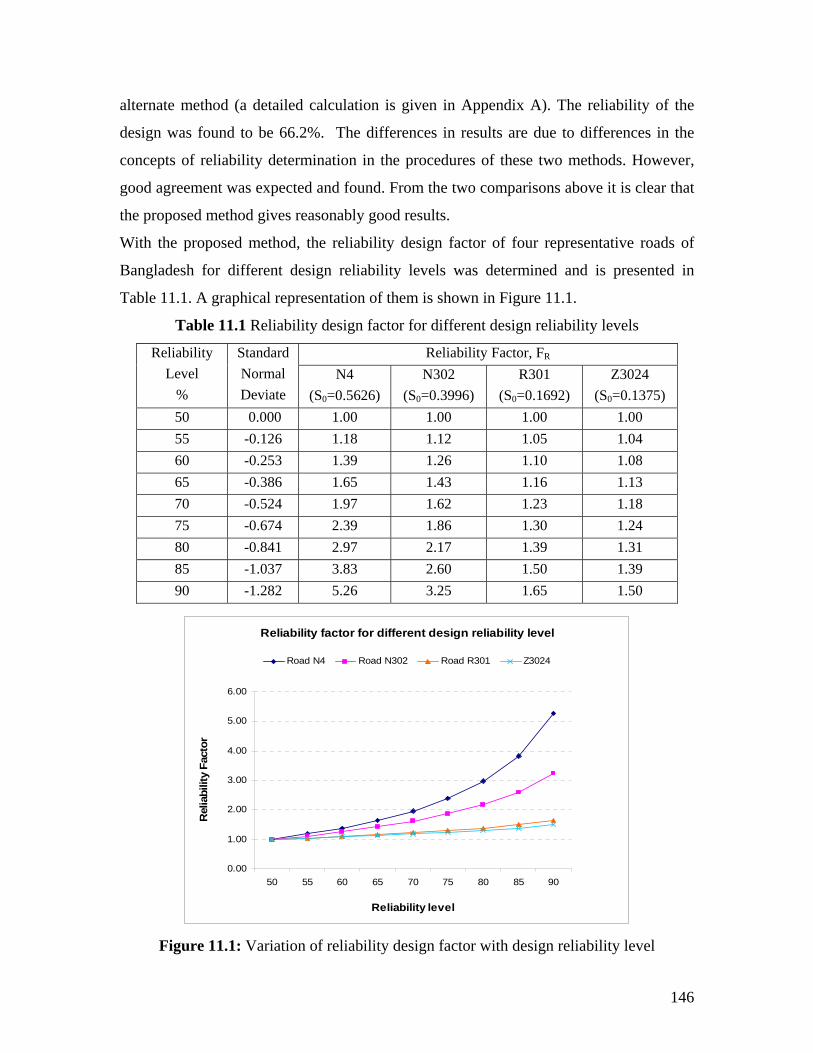
alternate method (a detailed calculation is given in Appendix A). The reliability of the
design was found to be 66.2%. The differences in results are due to differences in the
concepts of reliability determination in the procedures of these two methods. However,
good agreement was expected and found. From the two comparisons above it is clear that
the proposed method gives reasonably good results.
With the proposed method, the reliability design factor of four representative roads of
Bangladesh for different design reliability levels was determined and is presented in
Table 11.1. A graphical representation of them is shown in Figure 11.1.
Table 11.1 Reliability design factor for different design reliability levels
Reliability Factor, FR Reliability Level
%
Standard Normal Deviate
N4 (S0=0.5626)
N302 (S0=0.3996)
R301 (S0=0.1692)
Z3024 (S0=0.1375)
50 0.000 1.00 1.00 1.00 1.00 55 -0.126 1.18 1.12 1.05 1.04 60 -0.253 1.39 1.26 1.10 1.08 65 -0.386 1.65 1.43 1.16 1.13 70 -0.524 1.97 1.62 1.23 1.18 75 -0.674 2.39 1.86 1.30 1.24 80 -0.841 2.97 2.17 1.39 1.31 85 -1.037 3.83 2.60 1.50 1.39 90 -1.282 5.26 3.25 1.65 1.50
Reliability factor for different design reliability level
4.00
5.00
6.00
ctor
Road N4 Road N302 Road R301 Z3024
0.00
1.00
2.00
3.00
50 55 60 65 70 75 80 85 90
Reliability level
Rel
iabi
lity
Fa
Figure 11.1: Variation of reliability design factor with design reliability level
146
The reliability factor as shown in Table 11.1 in different roads for different reliability
level is significantly different from each other. This is because the pavement layer
configuration in different types of road is different. Hence, the sensitivity of pavement
performance in different roads is found different. In high standard roads such as N4 and
N302 roads the overall variance is mostly influenced by variation in surface strength,
value of overall
variance r value
of re to at the pavement should be designed for more traffic capacity
than pr sinc traffi eliability × predic ffic.
11.4 Qu tificati mban nt design risk
Significant variability was also found in the embankment design data. Hence a
methodology was required to ify the n emban t design to the
variability in design data which took account of both slope stability and settlement. A
number of method found e literatu analysin bankment design risk
against slope stability and these were compar th respect to some criteria, such as
accuracy mple c tional dure, cap to addre the varia of the
design data and suitability for the conditions in Bangladesh, so as to select or develop the
most suitable method (discussed in some detail in Chapter 6). The first order second
moment method was found to satisfy all the required criteria and the method was held to
be widely used and well recognized. The detailed procedure for this method was
discussed in section 6.2.2. The risk of N302 road embankment of Bangladesh was
analyzed with this method, on the basis of field and laboratory test data, as presented in
Chapter 7. The reliability of the N302 road embankment against slope stability was found
to be 63%. A procedure was also suggested to incorporate the desired reliability in design
against slope stability failure. The required value of the mean factor of safety for different
desired reliability levels against slope stability was also determined for the N302 road
embankment and presented in Table 7.3.
base strength and surface thickness and the value of overall variance consequently the
reliability factor is significant whereas in case of R301 and Z3024 roads the overall
variance is mostly influenced by variation in traffic parameters and the
and reliability factor is not so significant as high standard road. The highe
liability fac
edicted
r means th
e, design c = r factor ted tra
an on of e kme
quant risk i kmen due
s were in th re for g em
ed wi
, si omputa proce acity ss all bility
147
To find a way to quantify the embankment design risk against settlement the existing
literature was reviewed, but no method was found to be perfectly suitable for Bangladesh.
Hence, a method was developed in this research based on first order second moment
theory to quantify the embankment design risk against settlement. The first order second
moment theory was considered because it is simple, easy to understand, requires no
computer program, capable of accommodating all the variability of settlement and
suitable for the conditions in Bangladesh, not least because it uses data which are
available there. This theory is widely used and well recognized. Moreover, the same
theory is used for analyzing the risk in embankment slope stability. Hence, to maintain
consistency the theory was also selected for settlement risk analysis. The detailed
procedure of embankment settlement risk analysis with the proposed first order second
moment theory was presented in section 6.3.2. The risk of N302 road embankment
od and was found to be 85.5%. A
ssible outcomes which could occur when the
pavement and embankment performance were assessed together. The overall risk of the
against settlement was analyzed according to this meth
procedure was also suggested for incorporating the desired reliability in design against
settlement failure. The maximum allowable mean predicted settlement for various desired
reliability levels against settlement was also determined for the N302 road embankment
and presented in Table 7.4.
11.5 Quantification of overall design risk
In Bangladesh, pavements are usually built on embankments. The embankment acts as an
integral part of the pavement. The unsatisfactory performance of embankment as a result
of the variability in design data also influences the performance of pavement. Hence, the
overall risk of pavement embankment design system of Bangladesh associated with data
variability had to be quantified. A methodology was developed in this research to
quantify the overall risk based on the special multiplication rules of probabilities, as
discussed in some detail in Chapter 6. In the proposed methodology, the overall risk of
embankment design was first quantified by multiplying the probabilities of failure of
embankment design against slope stability by the probabilities of failure of embankment
design against settlement. Then the overall risk of the pavement embankment design
system was quantified, considering all po
148
design system of road N302 was quantified with this proposed procedure. The overall
risk of N302 road embankment was found to be 90.86% having a 37% risk against slope
stability and a 85.5% risk against settlement. Then, considering the risk of the pavement
design (25%) and the risk of the embankment (90.86%), the overall risk of a pavement
embankment design system for the worst possible outcome was found to be 93.15%.
11.6 Quality control process for Pavement and embankment construction
One of the objectives of this research is to incorporate a quality control system in the
design system of Bangladesh to reduce the variability in design data. To this end, a
quality control system for pavement design and a quality control procedure for
embankment design were developed in this research.
11.6.1 Quality control system for pavement
To develop a suitable quality control procedure for the proposed design system of
Bangladesh, the available methods and techniques were first investigated, but no
complete procedure was found in the literature. However, significant research work was
found on different components of quality control procedure, such as quality control tests,
test frequency and sampling, quality measures and performance relationship, which were
ts for Bangladesh. The Falling Weight
Bangladesh which made provision for a quality check after the construction of every
then compared to identify suitable componen
Deflectometer (FWD) or Benkelman Beam was identified as suitable methods for
evaluating pavement layer strength. Stratified random sampling, it was found, better
represents the pavement data. Mean and standard deviation was identified as a suitable
measure in determining the population mean of quality characteristics from the sample
mean. The t-test was also identified as a suitable means for establishing a confidence
interval of the sample mean. Since the proposed design for Bangladesh is an analytical
pavement design, the evaluation of a critical number of load repetitions before failure by
structural analysis was identified as the best measure of pavement performance. Having
identified the suitable components, the study developed a complete performance based
quality control procedure for Bangladesh; it is presented in section 8.5.1. The proposed
procedure included provision for pay adjustment if the work slightly deviated from
specification. The study also proposed a step-by-step quality control process for
149
layer to avoid disputes between the road agency and the contractor. The procedure was
presented in section 8.5.2. All the developed procedures were verified with field data.
11.6.2 Quality control system for Embankments
The pavement in Bangladesh is usually constructed out of soft sedimentary rock. Hence a
special provision was made in the proposed quality control procedure in this regard. The
tain
.
ure
Dynamic Cone Penetrometer (DCP) was identified as simple, easy to use and main
and cost effective. Consequently, it was suggested that the stability and uniformity of
embankment be checked with DCP tests. Personnel training and test strip construction
were identified as important components of embankment construction quality control and
provision was made for them in the proposed procedure
11.7 Applicability of the proposed proced
All the proposed procedures are simple to use, data demanding, applicable with the
proposed design system of Bangladesh and, most importantly, suitable for the prevailing
conditions in Bangladesh; for instance they use the available data and distress mode.
However, to judge the applicability of the proposed procedure, the developed methods
were presented in a workshop which twenty-seven representative engineers (different
ranks from different regions of Bangladesh) of the roads and highways department
(RHD) of Bangladesh attended. After the presentation a questionnaire survey was
conducted among them about the suitability and applicability of the proposed method
since it is they who will ultimately use it. More than 80% of them responded that the
procedure was clear and one which they liked. No one disliked the procedure. A good
proportion (75%) of them agreed that the procedure covers all the fundamental design
issues and 63% responded that the procedure is simple. Around 70% of the respondents
agreed that the procedure is appropriate for Bangladesh and more than 50% disagreed
with the view that the procedure is too theoretical. However, a considerable proportion of
them (15%-26%) responded ‘neither agree nor disagree’ to some of the questions. This
may be due to their not understanding the procedure since the reliability method is not
used before in the design system of Bangladesh. After proper training, however, they will
understand the procedure and it is hoped that they will respond positively. A summary of
the survey results is presented in Table 11.2.
150
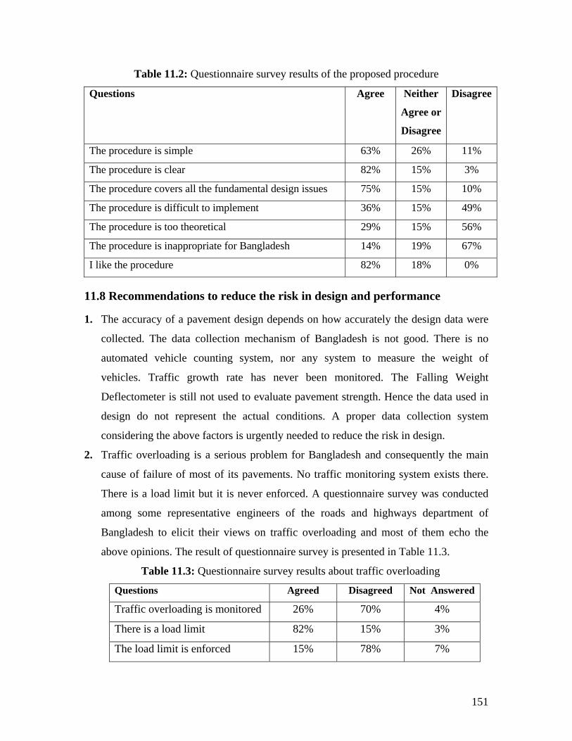
Table 11.2: Questionnaire survey results of the proposed procedure
Questions Agree Neither Disag
Agree or
Disagree
ree
The procedure is simple 63% 26% 11%
The procedure is clear 82% 15% 3%
The procedure covers all the fundamental design issues 75% 15% 10%
The procedure is difficult to implement 36% 15% 49%
The procedure is too theoretical 29% 15% 56%
The procedure is inappropriate for Bangladesh 14% 19% 67%
I like the procedure 82% 18% 0%
11.8 Recommendations to reduce the risk in design and performance
1. The accuracy of a pavement design depends on how accurately the design data were
collected. The data collection mechanism of Bangladesh is not good. There is no
automated vehicle counting system, nor any system to measure the weight of
vehicles. Traffic growth rate has never been monitored. The Falling Weight
Deflectometer is still not used to evaluate pavement strength. Hence the data used in
design do not represent the actual conditions. A proper data collection system
considering the above factors is urgently needed to reduce the risk in design.
2. Traffic overloading is a serious problem for Bangladesh and consequently the main
cause of failure of most of its pavements. No traffic monitoring system exists there.
There is a load limit but it is never enforced. A questionnaire survey was conducted
among some representative engineers of the roads and highways department of
Bangladesh to elicit their views on traffic overloading and most of them echo the
above opinions. The result of questionnaire survey is presented in Table 11.3.
Table 11.3: Questionnaire survey results about traffic overloading
Questions Agreed Disagreed Not Answered
Traffic overloading is monitored 26% 70% 4%
There is a load limit 82% 15% 3%
The load limit is enforced 15% 78% 7%
151
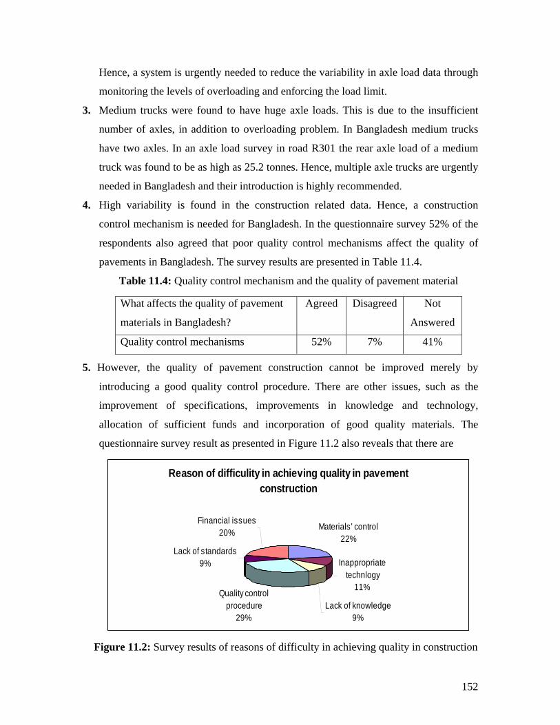
Hence, a through
ng the levels of overloading and enforcing the lo
3. Medium trucks were found to have huge axle loads. This is due to the insufficient
number of axles, in addition to overloading problem. In Banglad m trucks
axle load survey in road R301 the axle l f a m
e as high as 25.2 tonnes. Hence, mul xle tr re urg y
ly rec nded.
4 onstruction related data. Hence, a construction
for Bangladesh. In the ques aire survey 52% of the
control mechanisms affect the quality of
gladesh. The survey results are presented in Table 11.4.
terial
a system is urgently needed to reduce the variability in axle load dat
monitori ad limit.
esh mediu
have two axles. In an rear oad o edium
truck was found to b tiple a ucks a entl
needed in Bangladesh and their introduction is high omme
. High variability is found in the c
control mechanism is needed tionn
respondents also agreed that poor quality
pavements in Ban
Table 11.4: Quality control mechanism and the quality of pavement ma
What affects the quality of pavement
materials in Bangladesh?
Agreed Disagreed Not
Answered
Quality control mechanisms 52% 7% 41%
5. However, the quality of pavement construction cannot be improved merely by
introducing a good quality control procedure. There are other issues, such as the
improvement of specifications, improvements in knowledge and technology,
allocation of sufficient funds and incorporation of good quality materials. The
questionnaire survey result as presented in Figure 11.2 also reveals that there are
Reason of difficulity in achieving quality in pavement construction
Materials' control22%
Financial issues20%
Inappropriate Lack of standards
9%technlogy
11%
Lack of k dgeol
procedure29%
nowle9%
Quality contr
Figure 11.2: Survey results of reasons of difficulty in achieving quality in construction
152
other issues in addition to the quality control procedures which affect the quality of
pavement construction of Bangladesh.
6. A database of all design parameters is needed. It will enhance the variability
quantification and risk assessment system of Bangladesh.
7. The country requires a proper risk quantification methodology. The methodology
which is developed in this research is strongly recommended for it.
8. The study recommended the training of field staff to obtain a good data.
develop a
da isk
ba ta.
• De ce model for Bangladesh by performi tri-
ax ferences bet test c ions an ervice
conditions
•
The study makes the following recommendations for further research on quality control
procedures:
• Development of a complete specification and implementation guide for the quality
control of pavement and embankment construction in Bangladesh.
• A complete life cycle cost analysis of some of the country’s representative
pavements and embankments to allow it to develop its own pay adjustment factors.
11.10 Summary
The chapter has discussed the overall variability of the data found in Bangladesh, the
11.9 Recommendations for further research
The study makes the following recommendations for further research into risk analysis:
• A long term performance study of representative roads of Bangladesh to
tabase on long term performance and then work to determine the design r
sed on those long term performance da
velopment of a performan ng repeated
ial tests considering the dif ween ondit d in-s
• A comparative study of as build pavement thickness with as designed of some
representative roads of Bangladesh to determine the variability in the construction
related data.
A detailed questionnaire survey to assess the training needs of the personnel
involved in the process of data collection and risk analysis.
procedure for quantifying pavement and embankment design risk and a procedure of
153

con
Ban ound in a typical road in Bangladesh and the
pro d out in this study and the
reli investigation is
ality control
procedures.
struction quality control. These were developed or identified in this research for
gladesh. It has also outlined the risk f
general findings of the study. The acceptability of the proposed method among the
spective users was also discussed. The investigation carrie
consequent findings identified the topics which should be implemented to improve the
ability of design. Some areas were also identified where further
needed to refine the risk quantification process of the design system and qu
154
Chapter 12 Conclusions This thesis presented a comprehensive methodology to quantify the pavement and
embankment design risk associated with variability in data and a procedure for pavement
and embankment construction quality control. The proposed methodology and procedures
were developed with particular reference to the conditions in Bangladesh. The risk
analysis methodology and quality control procedure will enable the design system of
Bangladesh to incorporate reliability in design and to improve performance. The
following conclusions may be drawn from this study:
Variability of Data
1. No comprehensive database was avai ble in Bangladesh.
2. A database of pavement and embankment design parameter was established by
means of results from field and laboratory tests.
3. The data were found to be extremely variable. The data on the COV of pavement
layer thickness varied from 30%-50% and the COV of pavement layer strength
data varied from 0.63%-89.34%. Significant variability was found in the data on
embankment slope stability with COV ranging from 20% to 50%. At the same
time, embankment settlement data showed tremendous variability with COV in
some cases exceeding 100%.
4. Insufficient axle and overloading problems were found in the traffic data
5. Medium trucks were identified as contributing maximum damage with EALF =
7.205
6. DCP tests data were found to give highly variable results and are not suitable for
pavement layer strength evaluation.
Quantification of pavement design risk
1. The investigation of available methods revealed that no method was completely
suitable for the pavement design system of Bangladesh to quantify the risk
associated with the variability in design data.
2. A risk quantification method suitable for pavement design system of Bangladesh
was developed.
la
155
3. In calculating the prediction, a pavement
structural analysis model based on the method of equivalent thickness was
g with it other methods.
ocedure was also proposed to determine the risk of an existing
d methods that the first order
bankment of Bangladesh (N302) was found to be
kment design for both slope stability and settlement.
calculate the overall risk of a pavement
special multiplication rules of probabilities.
s found to be 93.15%.
t Deflectometer was identified as suitable for evaluating the
strength of pavement layers in Bangladesh.
variance in pavement performance
developed and used in the proposed procedure to make it compatible with the
proposed pavement design system of Bangladesh.
4. The risk of a typical pavement in Bangladesh was quantified with the proposed
method and the reliability factor was found to be 1.86 for a 75% reliability level,
which means the pavement should be designed for a capacity of 1.86 times the
predicted traffic to achieve 75% reliability in design.
5. The proposed method was verified by comparin
6. An alternative pr
structure.
Quantification of embankment design risk
1. It was identified by investigating the develope
second moment method is suitable for Bangladesh in calculating the embankment
design risk against slope stability.
2. A method of analysing embankment settlement risk was also proposed in this
research, using first order second moment theory, having investigated the
available methods.
3. The risk of a typical road em
37% for slope stability and 85.5% for settlement.
4. A procedure was also presented to incorporate the desired reliability in
emban
Quantification of overall risk
1. A methodology was developed to
embankment design system using the
2. The overall risk of embankment design of a typical road N302 of Bangladesh was
found to be 90.86% and the overall risk of a pavement embankment design
system for the worst combination of failure wa
Quality control of pavement construction
1. A Falling Weigh
156
2. To evaluate the pavement layer thickness on a mass scale, DCP tests were also
identified as suitable.
3. Stratified random sampling was identified as suitable for the quality control tests
of pavement construction in Bangladesh.
4. Mean and standard deviation was identified as a suitable measure in determining
the population mean of quality characteristics from the sample mean.
5. The t-test was selected as suitable for the quality control system of Bangladesh, to
establish a confidence interval of the sample mean.
6. The evaluation of pavement capacity in terms of the critical number of load
identified as the best way to establish performance relationship in the
onents of a quality control process for the
gladesh to avoid disputes between the road agency and
n the DCP index were selected as suitable measures for
e quality
t encourages a better product and helps in
repetitions that a pavement can sustain before failure with the quality control test
results was
country’s quality control process.
7. Pay adjustment provision was found to be suitable for Bangladesh
8. A performance based quality control process was developed in this research,
using the identified suitable comp
country, as mentioned above.
9. A quality control process after the completion of every layer was also identified
as suitable for Ban
contractors.
Quality control of embankment construction
1. Moisture content, density, stability and uniformity tests were identified as suitable
quality control tests for an embankment.
2. DCP index and variation i
the stability and uniformity of an embankment
3. The provision of test strip construction to determine the required rolling patterns,
number of roller passes and lift thickness was identified as suitable for
embankment construction quality control
4. A form of pay adjustment provision was identified as suitable for th
control system of Bangladesh, since i
resolving disputes.
157

Applicability of the proposed procedures
1. All the proposed procedures are simple, data demanding, suitable for the
he prospective users of these procedures
procedures
ife cycle cost analysis of different representative roads to develop
agencies, in order to develop a good
conditions in Bangladesh and applicable to the proposed design system.
2. The proposed procures was also liked by t
since almost 70%-80% of them responded positively in a questionnaire survey.
3. A training programme will increase the applicability of the proposed
since a reasonable proportion (15%-26%) of the respondents avoided giving exact
answers.
Need for improvement in the following areas to reduce the risk
1. Control mechanism for data collection
2. Control mechanism for traffic
3. Construction control mechanism
4. Database and specifications
5. Strategy for managing road maintenance
6. Technology and skills in terms of training
Need for work on the following projects:
1. A long term pavement performance study of representative roads of Bangladesh.
2. A detailed questionnaire survey to assess the training needs
3. A complete l
Bangladesh’s own pay adjustment factors.
4. A comparative study of the specification guide and implementation manuals for
quality control from different highway
standard for Bangladesh.
158
REFERENCES
merican
n
mplementation Manual for Quality Assurance - A Report of the
ssociation of State
gton, D.C.
Guide Specification - A Report of the AASHTO
, American Association of State Highway and
, D.C.
HIBLI, K. AND. SEYMAN, E. [2005].
n Pavement Construction Control.”
ransportation Research Board, National
ournal of Geotechnical Engineering,
ol. 26, Issue.3, pp.453-72.
L-QADI, I. L., LAHOUAR, S. AND. LOULIZI, AMARA. [2003]. “Successful
pplication of Ground-Penetrating Radar for Quality Assurance-Quality Control of New
avements.” Transportation Research Record 1861, Transportation Research Board,
ational Research Council, Washington, D.C., pp. 86-97.
L-QADI, I. L., LAHOUAR, S., JIANG, K., MCGHEE, K. K. AND. MOKAREM, D.
005]. “Accuracy of Ground-Penetrating Radar for Estimating Rigid and Flexible
AASHTO. [1993]. AASHTO Guide for Design of Pavement Structures. A
Association of State Highway and Transportation Officials, Washington, D.C.
AASHTO. [1986]. AASHTO Guide for Design of Pavement Structures. America
Association of State Highway and Transportation Officials, Volume-2, Washington, D.C.
AASHTO. [1996]. I
AASHTO Highway Subcommittee on Construction, American A
Highway and Transportation Officials, Washin
AASHTO. [1996]. Quality Assurance
Highway Subcommittee on Construction
Transportation Officials, Washington
ABU-FARSAKH, M. Y., NAZZAL, M. D., ALS
“Application of Dynamic Cone Penetrometer i
Transportation Research Record 1913, T
Research Council, Washington, D.C., pp. 53-61.
AGRAWAL, G. AND. ALTSCHAEFFL, A.G. [1991]. “Effect of Water-Content
Variability in Design of Clay Embankments.” J
Vol.117, N0.4, April, 1991, American Society of Civil Engineers, pp 673-683.
ALONSO, E. [1976]. “Risk Analysis of Slopes and Its Application to Slopes in Canadian
Sensitive Clays.” Geotechnique, V
A
A
P
N
A
[2
159

Pavement Layer Thicknesses.” h Record 1940, Transportation
esearch Board, National Research Council, Washington, D.C., pp. 69-78.
ay, 1988,
.
Transportation Research Board, National
GH, M. M. AND. LADD, C. C. [1983]. “Corrected Field Vane
SARMA, S. [1989] “Factor of Safety and Probability
y Experimental Design, 2nd Edition. Marcel Dekker,
Geotechnics, Vol.30, pp 455-462.
Transportation Researc
R
ALSHERRI, A. AND. GEORGE, K. P. [1988]. “Reliability Model for Pavement
Performance.” Journal of Transportation Engineering, Vol.114, No.2, M
American Society of Civil Engineers, pp 294-307.
ASPHALT INSTITUTE [1981]. Thickness Design - Asphalt Pavements for Highways
and Streets. Manual Series No. 1 (MS-1), The Asphalt Institute.
ATKINSON, J. [2007]. The Mechanics of Soils and Foundations, 2nd edition, Taylor &
Francis, 2 Park Square, Milton Park, Abingdon, Oxon, UK
ATTOH-OKINE, N. O. AND RODDIS, W. M. K. [1994]. “Pavement Thickness
Variability and its Effect on Determination of Moduli and Remaining Life.”
Transportation Research Record 1449,
Research Council, Washington, D.C., pp 39-45.
AUSTROADS. [2004]. Pavement Design-A Guide to the Structural Design of Road
Pavements. ARRB Transport Research, Austroads Incorporated, Sydney, Australia.
AZZOUS, A. S., BALI
Strength for Embankment Design.” Journal of Geotechnical Engineering, Vol.109, No. 5,
American Society of Civil Engineers, pp 730-734.
BARABOSA, M., MORRIS, D.,
of Failure of Rockfill Embankments.” Geotechnique, Vol. 39, Issue3, pp 471-483.
BARKER, T. B. [1994]. Quality b
Inc., New York.
BARNES, G. E. [1995]. Soil Mechanics-Principles and Practice. MacMillan Press Ltd,
Houndmills, Basingstoke, Hampshire.
BHATTACHARYA, G., JANA, D., OJHA, S. AND. CHAKRABORTY, S [2003].
“Direct Search for Minimum Reliability Index of Earth Slopes.” Computers and
160
BISHOP, A. W. [1955]. “The Use of the Slip Circle in the Stability Analysis of Slopes.”
Geotechnique, London, 5(1), pp 7-17.
BROWN, J. L. [1994]. “Reliability in Pavement Design? Who’s Kidding Whom?”
Transportation Research Record 1449, Transportation Research Board, National
Research Council, Washington, D.C., pp 26-29.
BROWN, J. L. AND. BUTTLER, L. J. [1970]. “A Recommended Texas Highway
Department Pavement Design System User’s Manual.” Texas Highway Department
elopment to the th
6] “Accuracy and Precision of Typical
ion Engineering, Vol. 125, No. 2,
esting
and Evaluation, Vol. 35, No. 2.
and Subgrade layers” Transportation Research
National Research Council, Washington,
ial Variability of Soil Properties on Slope Stability.”
Research Report 123-2, Texas Highway Department.
BRUNTON, J. M., BROWN, S.F. AND. PELL, P.S. [1987]. “Dev
Nottingham Analytical Design Method for Asphalt Pavements.” Proceeding of the 6
International Conference on Structural Design of Asphalt Pavements, Vol. 1, ISAP, 366-
377.
BURATI J. L., JR., AND WEED R. M. [200
Quality Measures.” Transportation Research Record 1946, Transportation Research
Board, National Research Council, Washington, D.C., pp 82-91.
BURR, I. W. [1976]. Statistical Quality Methods. Marcel Dekker, Inc., New York.
CASTELL, M.A. AND. PINTADO, P. [1999]. “Sensitivity Analysis for Estimation of
Pavement Fatigue Life.” Journal of Transportat
March/April 1999, American Society of Civil Engineers, pp 114-122.
CHEN, D. H. AND. SCULLION, T. [2006]. “Using Nondestructive T
Technologies to Assist in Selecting the Optimal Pavement Rehabilitation Strategy.”
Journal of Testing
CHEN, D. -H., WANG, J. -N. AND. BILYEU, J. [2001]. “Application of Dynamic Cone
Penetrometer in Evaluation of Base
Record 1764, Transportation Research Board,
D.C., pp. 1-10.
CHO, S. E. [2007]. “Effects of Spat
Engineering Geology, Vol. 92, pp 97-109.
161
CHOWDHURY, R. N. AND. XU, D.W. [1995]. “Geotechnical System Reliability of
Slopes.” Reliability Engineering and System Safety, Issue 47, pp 141-151.
ineers, Geotechnical Special Publication
l Engineering, Vol.120, No. 12,
eering, Vol.130, No. 10, October, 2004, American Society of Civil Engineers, pp
eering, Vol.118, No.6,
Required Falling
7]. Principles of Geotechnical Engineering, 4th Edition, PWS Publishing
CHRISTIAN, J. T. [1996]. “Reliability Methods for Stability of Existing Slopes.” In
Uncertainty in the Geological Environment: From Theory to Practice, Proceedings of
Uncertainty’96, American Society of Civil Eng
No. 58, C.D. Shackelford, P.P Nelson, and M.J.S. Roth, eds., pp. 409-418.
CHRISTIAN, J. T., LADD, C. C.AND. BAECHER, G. B. [1994]. “Reliability Applied to
Slope Stability Analysis.” Journal of Geotechnica
December, 1994, American Society of Civil Engineers, pp 2180-2207.
CHRISTIAN, J. T. [2004]. “Geotechnical Engineering Reliability: How well do We
Know What We Are Doing?” Journal of Geotechnical and Geoenvironmental
Engin
985-1003.
CHUA, K. H., KIUREGHIAN, A. D. AND. MONISMITH, C. L [1992]. “Stochastic
Model for Pavement Design.” Journal of Transportation Engin
November/December, 1992, American Society of Civil Engineers, pp 769-785.
CRAIG, R. F. [2004]. Craig’s Soil Mechanics. Spon Press, Taylor & Francis Group,
London and New York.
DAMNJANOVIC, I. AND. ZHANG, Z. [2006]. “Determination of
Weight Deflectometer Testing Frequency for Pavement Structural Evaluation at the
Network Level.” Journal of Transportation Engineering, Vol.132, No.1, January, 2006,
American Society of Civil Engineers, pp 76-85.
DAS, A. AND. PANDEY, B. B. [1999] “Mechanistic-Empirical Design of Bituminous
Roads: An Indian Perspective.” Journal of Transportation Engineering, Vol.125, No.5,
September/October 1999, American Society of Civil Engineers, pp 463-471.
DAS, B. M. [199
Company, 20 Park Plaza, Boston.
162
D’ Andrea, R. [2001]. Discussion of “Search Algorithm for Minimum Reliability Index
of Earth Slopes.” By Hassan and Wolff, Journal of Geotechnical and Geoenvironmental
D.C., pp 111-
rance for Asphalt
, K. D., COPLANTZ, J., LEHMANN, R. AND. BRESSETTE, T. [1999]
. CRUDEN, D. M. [2003]. Reply to the
robabilistic
Engineering, Vol.127, No. 2, American Society of Civil Engineers, pp 195-197.
DEMPSEY, B. J., HERLACHE, W. A., AND PATEL, A. J. [2006]. “Climate-Materials-
Structural Pavement Analysis Program.” Transportation Research Record 1095,
Transportation Research Board, National Research Council, Washington,
118.
DOBROWOLSKI, J. AND. BRESSETTE, T. [1998]. “Development of Quality Control/
Quality Assurance Specifications by Using Statistical Quality Assu
Concrete Pavements in California.” Transportation Research Record 1632,
Transportation Research Board, National Research Council, Washington, D.C., pp. 13-
21.
DOUGLAS
“Evaluation of Quality Control / Quality Assurance Implementation for Asphalt Concrete
Specification in California.” Transportation Research Record 1654, Transportation
Research Board, National Research Council, Washington, D.C., pp. 95-101.
DUNCAN, A. J. [1974]. Quality Control and Industrial Statistics. 4th Edition. Richard D.
Irwin, Inc., Homewood, IL.
DUNCAN, J. M., NAVIN, M. AND. WOLFF, T. F. [2003]. “Discussion of Probabilistic
Slope Stability Analysis for Practice” Canadian Geotechnical Journal, Vol.40 pp 848-
850.
EI-RAMLY, H., MORGENSTERN, N. R. AND
Discussion by J.M. Duncan, M. Navin, and T.F. Wolff on ‘Probabilistic Slope Stability
Analysis for Practice’ Canadian Geotechnical Journal, Vol.40 pp 851-855.
EI-RAMLY, H., MORGENSTERN, N. R. AND. CRUDEN, D. M. [2002]. “P
Slope Stability analysis for Practice.” Canadian geotechnical Journal, Vol. 39, pp 665-
683.
163
ELLIS, C. I. [1975]. “Risk and the Pavement Design Decision in Developing Countries.”
TRRL Laboratory Report 667, Department of the Environment, Transport and Road
Research Laboratory, Crowthorne, Berkshire.
EVDORIDES, H. [2007]. “Notes on Pavement Analysis and Evaluation.” Lecture Note,
School of Engineering, University of Birmingham, March 2007.
FENTON, G. A. AND. GRIFFITHS, D. V. [2002]. “Probabilistic Foundation Settlement
on a Spatially Random Soil.” Journal of Geotechnical and Geo-environmental
entary Statistics. Fifth Edition, Prentice-Hall, INC.,
al of Geotechnical and Geo-environmental Engineering,
erican Society of Civil Engineers, pp 507-518.
ents.” Geotechnique, Vol. 48, No.3, pp 387-403.
FER, A. M. AND. LIND, N. [1974]. “Exact and Invariant Second-Moment Code
at.” Journal of Engineering Mechanics, Vol. 100, No.1, pp 111-121.
Engineering, Vol.128, No. 5, American Society of Civil Engineers, pp 381-390.
FOOTT, R. AND. LADD, C. C. [1981]. “Undrained Settlement of Plastic and Organic
Clays.” Journal of the Geotechnical Engineering Division, Proceedings of the American
Society of Civil Engineers, ASCE, Vol. 107, No. GT8, August 1981.
FREUND, J. E. [1979]. Modern Elem
Englewood Cliffs, New Jersey.
GRANT, E. L., AND LEAVENWORTH R. S. [1980]. Statistical Quality Control. 5th
Edition. McGraw-Hill, Inc., New York.
GRIFFITHS, D. V. AND. FENTON, G.A. [2004]. “Probabilistic Slope Stability Analysis
by Finite Elements.” Journ
Vol.130, No. 5, Am
GRIFFITHS, D. V. AND. LANE, P.A. [1999]. “Slope Stability Analysis by Finite
Elem
HARISON, J. A. [1987]. “Correlation between California Bearing Ratio and Dynamic
Cone Penetrometer Strength Measurement of Soils.” In Proceedings of Institution of
Civil Engineers, Part 2, 1987, 83, Dec., 833-844, Technical note 463.
HARR, M. E. [1987]. Reliability-Based Design in Civil Engineering, McGraw-Hill, New
York.
HASO
Form
164
HOUSTON, W. N., MAMLOUCK, M. S. AND. PERERA, R. W.S. [1992]. “Laboratory
versus Nondestructive Testing for Pavement Design.” Journal of Transportation
Engineering, Vol.118, No.2, March/April, 1992, American Society of Civil Engineers, pp
Hall, Englewood Cliffs,
ighway
ent Layer Thickness Variability for Reliability-Based
156-165.
ethod for Bangladesh.
robabilistic Concepts and Their
tivity Analysis of
ransportation Research Board, National Research Council, Washington, D.C., pp
207-222.
HUANG, Y. H. [1993]. Pavement Analysis and Design. Prentice-
N.J.
HUDSON, S. B. [1971]. Handbook of Applications of Statistical Concepts to the
Highway Industry, Part I – Initial Computations and Applications. Federal H
Administration, Washington, D.C.
JAMBU, N. [1968]. “Slope Stability Computations.” Soil Mechanics and Foundation
Engineering Report, The Technical University of Norway, Trondheim, Norway.
JIANG, Y. J., SELEZNEVA, O., MLADENOVIC, G., AREF, S. AND. DARTER, M.
[2003]. “Estimation of Pavem
Design.” Transportation Research Record 1849, Transportation Research Board, National
Research Council, Washington, D.C., pp
JUANG, C. H., JHI, Y. –Y.AND. LEE, D.-H [1998]. “Stability Analysis of Existing
Slopes Considering Uncertainty.” Engineering Geology, Vol. 49, pp 111-122.
KHAN, H. R. [2005]. A Prototype Analytical Pavement Design M
M. Phil dissertation, School of Engineering, University of Birmingham.
KHER, R. K. AND. DARTER, M. I. [1973]. “P
Applications to AASHO Interim Guide for Design of Rigid Pavements.” Highway
Research Record No. 466, Highway Research Board.
KILLINGSWORTH, B. M. AND ZOLLINGER D. G. [1995] “Sensi
Input Parameters for Pavement Design and Reliability.” Transportation Research Record
1482, T
111-122.
165
KIM, H. B. [2006]. “Practical Probabilistic Design Format for Flexible Pavements.”
Transportation Research Record 1947, Transportation Research Board, National
Research Council, Washington, D.C., pp185-192.
KIM, J.R.
, KANG, H. B., KIM, D., PARK, D. S.AND KIM, W. J.[2007]. “Evaluation of
late-Bearing Load Test” Journal of the Materials in Civil Engineering, Vol. 19,
ion and Utilization.” Transportation Research Record
ncertainties in Characterizing Soil
nsuitable Soils”.
of the 2007 Mid-Continent Transportation Research Symposium, Ames,
ents.” Highway Research Record No. 362, Highway Research Board.
olume 54, Issue 3-4, October 1999, pp 271-285.
LI, K.AND. LUMB, P. [1987]. “Probabilistic Design of Slopes.” Canadian Geotechnical
Journal, Vol.24, pp 520-535.
In Situ Modulus of Compacted Subgrades Using Portable Falling Weight Deflectometer
and P
No.6, June, 2007, American Society of Civil Engineers, pp 492-499.
KSAIBATI, K., McNAMARA, R., MILEY, W. AND ARMAGHANI, J. [1999].
“Pavement Roughness Data Collect
1655, Transportation Research Board, National Research Council, Washington, D.C., pp
86-92.
KULKARNI, R. B. [1994]. “Rational Approach in Applying Reliability Theory to
Pavement Structural Design.” Transportation Research Record 1449, Transportation
Research Board, National Research Council, Washington, D.C., pp 13-17.
LACASSE, S. AND. NADIM, F. [1996]. “U
Properties.” In proceedings of Uncertainty ‘96. Geotechnical Special Publication 58, Vol.
1, pp. 49–75.
LARSEN, B.W., WHITE, D.J. AND. JAHREN, C.T. [2007]. “Embankment Construction
QC/QA using DCP and Moisture Control: Iowa Case History for U
Proceedings
Iowa, August 2007.
LEMER, A. C. AND. NOAVENZADEH, F. [1971]. “Reliability of Highway
Pavem
LIANG, R. Y., NUSIER, O. K. AND. MALKAWI, A. H. [1999]. “A Reliability Based
Approach for Evaluating the Slope Stability of Embankment Dams.” Engineering
Geology, V
166
LUA, Y. J. AND. SUES, R. H. [1996]. “Probabilistic Finite-Element Analysis of Airfield
Pavements.” Transportation Research Record 1540, Transportation Research Board,
National Research Council, Washington, D.C., pp 29-38.
Iran and AASHTO
ity Analysis Applied to Slope Stability.” Structural Safety, Vol. 22, pp 161-187.
D.C., pp. 89-
of Pavements.” Journal of Materials in Civil Engineering, Vol. 15, No.1,
ANG, Y. J., SELEZNEVA, O., AREF, S. AND. DARTER, M.
rch Board,
.” International Symposium
LIVNEH, M. [2002]. “On the Acceptance Criteria for Statistical Quality Control in
Pavement Construction.” Presented for the 2002 Federal Aviation Administration Airport
Technology Transfer Conference.
MAHERI, M. AND AKBARI, R. [1993]. “Comparison Between
Codes with Considering Overloaded Trucks.” Proceedings 6th International Conference
of Civil Engineering, Vol.1, Isfehan University of Technology, Isfehan, Iran.
MALKAWI, A. I. H., HASSAN, W.F., ABDULLA, F.A. [2000]. “Uncertainty and
Reliabil
MARSHALL, C., MEIER, R. AND. WELCH, M. [2001]. “Seasonal Temperature Effects
on Flexible Pavements in Tennessee.” Transportation Research Record 1764,
Transportation Research Board, National Research Council, Washington,
96.
MEHTA, Y. AND. ROQUE, R. [2003]. “Evaluation of FWD Data for Determination of
Layer Moduli
February, 2003, American Society of Civil Engineers, pp 25-31.
MCELVANEY, J.AND. SNAITH, M. S. [2002]. Analytical Design of Flexible
Pavement. Butterworth-Heinemann, Linacre House, Jordan Hill, Oxford.
MLADENOVIC, G., JI
[2003]. “Comparison of As-Constructed and As-Designed Flexible Pavement Layer
Thicknesses.” Transportation Research Record 1853, Transportation Resea
National Research Council, Washington, D.C., pp. 165-175.
NAKAMURA, Y., KOJIMA, J., NARITA, K. AND. OHNE, Y. [1998]. “Quality Control
of High Embankments Constructed of Soft Sedimentary Rock
on Problematic Soils, 1998, Sendai, Japan, Problematic Soil, Vol 1, pp 701-704.
167
NATIONAL CO-OPERATIVE HIGHWAY RESEARCH PROJECT (NCHRP). [2004].
Guide for Mechanistic-Empirical Design of New and Rehabilitated Pavement Structures.
Final Report, Project 1-37A. TRB, National Research Council, Washington, D.C., March
2004 [e] http//trb.org/mepdg/guide.htm. Last accessed june15, 2009.
NOURELDIN, A. S., ZHU, K., LI, S., HARRIS, D. [2003]. “Network Pavement
Evaluation with Failing-Weight Deflectometer and Ground-Penetrating Radar.”
F. [1996].
ashington, D.C., pp 39-47.
g AASHTO Model.” Transportation Research Record 1449, Transportation Research
Washington, D.C., pp 46-56.
nd Soil Characteristics.”
ansportation Research Board, National
A. AND HONG, F. [2006]. “Seasonal Time Series Models to Support Traffic
CHER, M. AND. JACKSON, N.C [2006]. “Utilizing
Transportation Research Record 1860, Transportation Research Board, National
Research Council, Washington, D.C., pp. 90-99.
NOURELDIN, A. S., SHARAF, E., ARAFAH, A. AND. AL-SUGAIR,
“Rational Selection of Factors of Safety in Reliability-Based Design of Flexible
Pavements in Saudi Arabia.” Transportation Research Record 1540, Transportation
Research Board, National Research Council, W
NOURELDIN, A. S., SHARAF, E., ARAFAH, A. AND. AL-SUGAIR, F. [1994].
“Estimation of Standard Deviation of Predicted Performance of Flexible Pavements
Usin
Board, National Research Council,
OH, J., RYU, D., FERNANDO, E. G. AND LYTTON, R. L. [2006]. “Estimation of
Expected Moisture Contents for Pavements by Environmental a
Transportation Research Record 1967, Tr
Research Council, Washington, D.C., pp 135-147.
PROZZI, J.
Input Data for Mechanistic-Empirical Design Guide.” Transportation Research Record
1947, Transportation Research Board, National Research Council, Washington, D.C.,
pp175-184.
PAPAGIANNAKIS, A. T., BRA
Clustering Techniques in Estimating Traffic Data Input for Pavement Design.” Journal of
Transportation Engineering, Vol.132, No.11, November 2006, American Society of Civil
Engineers, pp 872-879.
168
PATEL, A. AND. THOMPSON, M. [1998]. “Consideration and Characterization of
Pavement Construction Variability.” Transportation Research Record 1632,
Transportation Research Board, National Research Council, Washington, D.C., pp. 40-
50.
PATHOMVANICH, S. [2000]. Assessment of the Effectiveness of Quality Assurance
Construction Specifications for Asphaltic Concrete Pavement. Ph.D. dissertation.
University of Florida.
RADA, G. AND. WITCZAK, M.W. [1981]. “Comprehensive Evaluation of Laboratory
robabilities.” Applied
atical Model, 5(2), pp329-335.
“Deterioration Analysis of Flexible
g –Term Pavement Performance Data to Predict Seasonal Variation in
rrent Quality Control/ Quality Assurance Practices for Hot-Mix
Resilient Moduli Results for Granular Material.” Transportation Research Record 810, pp
23-33.
RHD [2005]. Benkelman Beam Deflection Survey Manual, Roads and Highways
Department, Dhaka, Bangladesh, May 2005, pp 1-8.
RHD [2001]. Manual Classified Traffic Counts Instruction Guide, Roads and Highways
Department, Dhaka, Bangladesh, October 2001, pp 14.
ROSENBLUETH, E. [1981]. “Two-Point Estimates in P
Mathem
SAARENKETO, T.AND. SCULLION, T. [2000]. “Road Evaluation with Ground
Penetrating Radar.” Journal of Applied Geophysics, Issue 43, pp119–138
SADEGHI, J.M. AND FATHALI, M. [2007].
Pavements Under Overweight Vehicles.” Journal of Transportation Engineering,
Vol.133, No.11, November 2007, American Society of Civil Engineers, pp 625-633.
SALEM, H. M., BAYOMY, F. M., AL-TAHER, M. G. AND. GENC, I. H. [2004].
“Using Lon
Asphalt Concrete Modulus.” Transportation Research Record No. 1896, Transportation
Research Board, National Research Council, Washington, D.C., pp. 119-128.
SCHMITT, R. L., RUSSELL J. S., HANNA A. S., BAHIA H. U. AND JUNG G. A.
[1998]. “Summary of Cu
169
Asphalt Construction.” Transportation Research Record No. 1632, Transportation
Research Board, National Research Council, Washington, D.C., pp. 22-31.
SCHWARTZ C. W. [2007] “Implementation of the NCHRP 1-37A Design Guide.” Final
Report, Vol-1, Summary of Findings and Implementation Plan, Maryland State Highway
e University of Birmingham for the degree of M. Phil.
, FREER-HEWISH, R. J.AND. SHEIN, A. [1980].
om.
don, 17(1), pp 11-26
al Journal, Vol.13, Issue.3, pp 201-215.
Statistical Quality Assurance Methods
Administration, 2007. [e]
SHAHJAHAN, M. [2009]. Materials Considered for Pavement and Embankment Design.
A thesis submitted to th
SHELL PAVEMENT DESIGN MANUAL - ASPHALT PAVEMENTS AND
OVERLAYS FOR ROAD TRAFFIC [1978]. Shell International Petroleum Ltd., London.
SNAITH, M.S., McMULLEN, D.
“Flexible Pavement Analysis.” Final Technical Report, U.S. Army Research,
Development & Standardization Group, United Kingd
SPENCER, E. [1967]. “A Method of Analysis of the Stability of Embankments
Assuming Parallel Interslice Forces.” Geotechnique, Lon
TANG, W., YUCEMEN, M. AND. ANG A.-S. [1976]. “Probability-Based Short Term
Design of Slopes.” Canadian Geotechnic
TOMLINSON, M. J. [2001]. Foundation Design and Construction. Pearson Education
Limited, Edinburgh Gate, Harlow, Essex, England.
TORRES-VERDIN, V. AND McCULLOUGH, B. F. [1991]. “Dynamic Quality Control
of Flexible Pavement.” Journal of the Transportation Engineering, Volume 117,
American Society of Civil Engineers, pp 23-33.
TRL [1993]. A Guide to the Structural Design of Bitumen-surfaced Roads in Tropical
and Sub-tropical Countries, Overseas Centre, Transport Research Laboratory,
Crowthorne, Berkshire, United Kingdom.
VARDEMAN, S. B., AND JOBE, J. M. [1999].
for Engineers. John Wiley & Sons, Inc., New York.
170
VENMARCKE, E. [1977]. “Reliability of Earth Slopes.” Journal of Geotechnical
Engineering Division, American Society of Civil Engineers, Vol.103, Issue 11, pp 1247-
ol and Improvement. John Wiley & Sons, Inc., New York.
ch Board,
ashington, D.C., pp 63-70.
ent: Complete Development Process.” Transportation Research
Derivation of Equation for Cost of Premature Pavement Failure.”
National
lating As-Built Quality to Pavement
. AND. PERRY, E. [1996]. “Reliability
pecial Publication No. 58, C.D. Shackelford,
ponse Surface Method.” Journal of
erican Society of Civil Engineers, pp 32-
53.
1265.
WADSWORTH, H. M., KENNETH, S. S., AND GODFREY, A. B. [1986]. Modern
Methods for Quality Contr
WEED, R. M. [2006]. “Mathematical Modelling Procedures for Performance- Related
Specifications.” Transportation Research Record 1946, Transportation Resear
National Research Council, W
WEED, R. M. [2003]. “Multicharacteristic Performance-Related Specification for Hot-
Mix Asphalt Pavem
Record 1861, Transportation Research Board, National Research Council, Washington,
D.C., pp. 53-59.
WEED, R. M. [2001]. “
Transportation Research Record 1761, Transportation Research Board, National
Research Council, Washington, D.C., pp. 93-96.
WEED, R. M. [1999]. “Practical Framework for Performance-Related Specification.”
Transportation Research Record 1654, Transportation Research Board,
Research Council, Washington, D.C., pp. 81-87.
WEED, R. M. [1998]. “A Rational Method for Re
Performance and Value.” Transportation Research Record 1632, Transportation Research
Board, National Research Council, Washington, D.C., pp. 32-39.
WOLFF, T. F., DEMSKY, E. C., SCHAUER, J
Assessment of Dam and Levee Embankments.” In Uncertainty in the Geologic
Environment: From Theory to Practice, Proceedings of Uncertainty ’96, American
Society of Civil Engineers Geotechnical S
P.P Nelson, and M.J.S. Roth, eds., pp. 636-650.
WONG, F. S. [1985]. “Slope Reliability and Res
Geotechnical Engineering, Vol.111, No. 1, Am
171
WU, T. AND. KRAFT, L. [1970]. “Safety Analysis of Slopes.” Journal of Soil
Mechanics and Foundation Division, American Society of Civil Engineers, Vol.96, Issue
2, pp 609 -630.
tal
ples of Pavement Design. 2nd
search Board, National Research Council, Washington, D.C., pp. 1-12.
ivil Engineers, pp 416-424.
eers, pp 47-56.
XU, B. AND. LOW, B. K. [2006]. “Probabilistic Stability Analyses of Embankments
ased on Finite-Element Method.” Journal of Geotechnical and Geo-environmenB
Engineering, Vol.132, No. 11, November, 2006, American Society of Civil Engineers, pp
1444-1454.
YODER, E. J. AND. WITCZAK, M.W. [1975]. Princi
Edition, John Wiley & Sons, Inc., New York.
ZAGHLOUL, S., SAEEED, N.A., JASSIM, A.A. AND. RAFI, A. M. [1998]. “End-result
Specifications for Warranted Asphalt Pavements.” Transportation Research Record 1632,
Transportation Re
ZHANG, Z. AND. DAMNJANOVIC, I. [2006]. “Applying Method of Moments to
Model Reliability of Pavements Infrastructure.” Journal of Transportation Engineering,
Vol.132, No.5, May/2006, American Society of C
ZOU, J. –Z., WILLIAMS, D. J. AND. XIONG, W.-L.[1995]. “Search for Critical Slip
Surfaces Based on Finite Element Method.” Canadian Geotechnical Journal, Vol.32,
o.2 pp 233-246. N
ZUO, G., DRUMM, E. C. AND MEIER, R. W. [2007]. “Environmental Effects on the
Predicted Service Life of Flexible Pavements.” Journal of the Transportation
Engineering, Volume 133, No. 1, American Society of Civil Engin
172
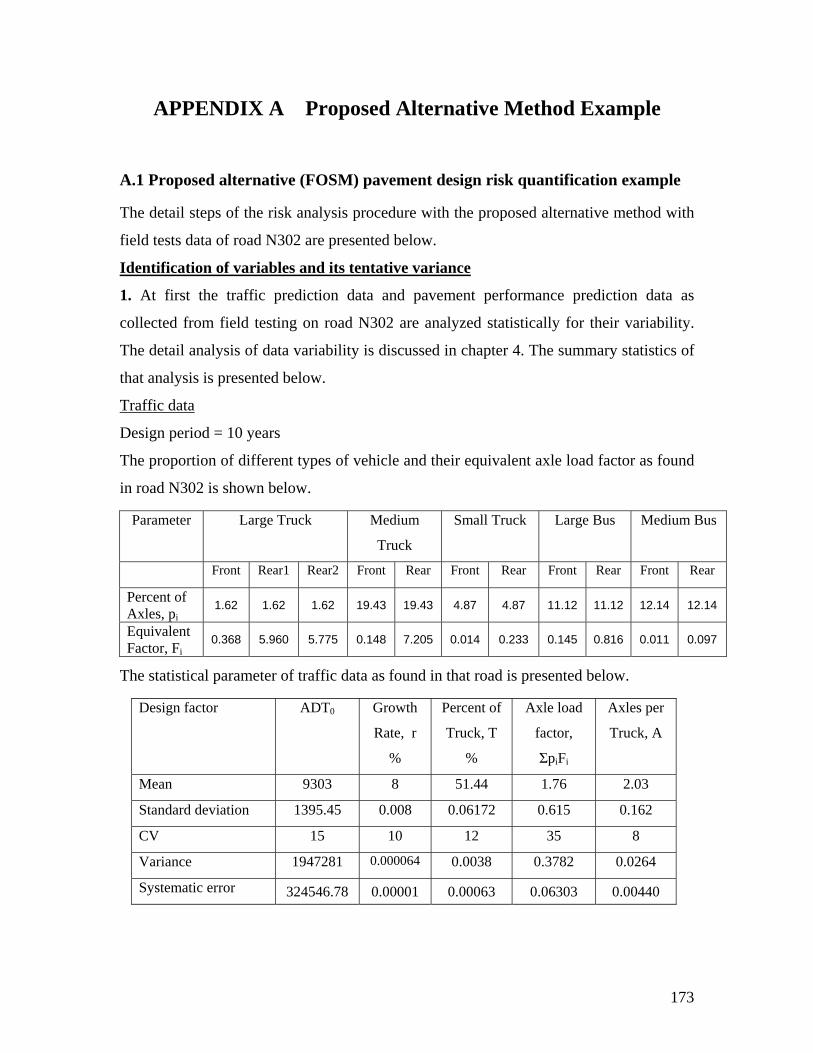
APPENDIX A Proposed Alternative Method Example
A.1 Proposed alternative (FOSM) pavement design risk quantification example
and its tentative variance
The detail steps of the risk analysis procedure with the proposed alternative method with
field tests data of road N302 are presented below.
Identification of variables
At first the traffic prediction data and pavement performance prediction data as
ed in chapter 4. The summary statistics of
1.
collected from field testing on road N302 are analyzed statistically for their variability.
The detail analysis of data variability is discuss
that analysis is presented below.
Traffic data
Design period = 10 years
The proportion of different types of vehicle and their equivalent axle load factor as found
in road N302 is shown below.
Parameter Large Truck Medium Small Truck Large Bus
Truck
Medium Bus
Front Rear1 Rear2 Front Rear Front Rear Front Rear Front Rear
Percent of Axles, pi
1.62 1.62 1.62 19.43 19.43 4.87 4.87 11.12 11.12 12.14 12.14
Equivalent Factor, Fi
0.368 5.960 5.775 0.148 7.205 0.014 0.233 0.145 0.816 0.011 0.097
The statistical parameter of traffic data as found in that road is presented below.
Design factor ADT0 Growth Percent of Axle load Axles p
Rate, r
%
Truck, T
%
factor,
ΣpiFi
er
Truck, A
Mean 9303 8 51.44 1.76 2.03
Standard deviation 1395.45 0.008 0.06172 0.615 0.162
CV 15 10 12 35 8
Variance 1947281 0.000064 0.0038 0.3782 0.0264
Systematic error 324546.78 0.00001 0.00063 0.06303 0.00440
173
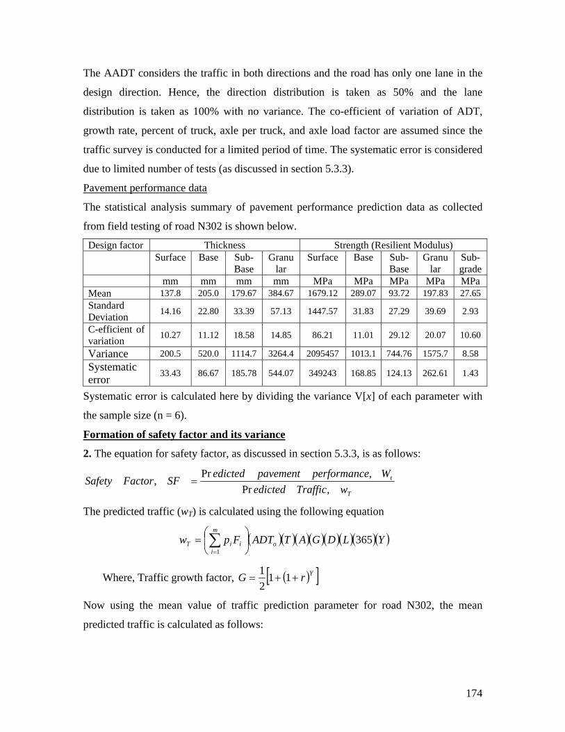
The the
design direction. Hence, the direction di tribution is taken as 50% and the lane
ce. The co-efficient of variation of ADT,
e
on 5.3.3).
AADT considers the traffic in both directions and the road has only one lane in
s
distribution is taken as 100% with no varian
growth rate, percent of truck, axle per truck, and axle load factor are assumed since th
traffic survey is conducted for a limited period of time. The systematic error is considered
due to limited number of tests (as discussed in secti
Pavement performance data
The statistical analysis summary of pavement performance prediction data as collected
from field testing of road N302 is shown below.
Design factor Thickness Strength (Resilient Modulus) Surface Base Sub-
Base Granu
lar Surface Base Sub-
Base Granu
lar Sub-grade
mm mm mm mm MPa MPa MPa MPa MPa Mean 137.8 205.0 179.67 384.67 1679.12 289.07 93.72 197.83 27.65 Standard Deviation 14.16 22.80 33.39 57.13 1447.57 31.83 27.29 39.69 2.93
C-efficient of variation 10.27 11.12 18.58 14.85 86.21 11.01 29.12 20.07 10.60
Variance 20 1114.7 20 .1 75.70.5 520.0 3264.4 95457 1013 744.76 15 8.58 S error 33.43 86.67 185.78 349243 168.85 124.13 262.61 1.43 ystematic 544.07
System tic err c e b d e c ] of each param it
t ize 6)
Formation of safety factor and its variance
a or is alculat d here y divi ing th varian e V[x eter w h
he sample s (n = .
2 ation for safety factor, as discussed in section 5.3.3, is as follows: . The equ
Twaffic,
llowing e
tWeperformancpavementedicted ,PrTre
SFFactorSafetyPr
, =
The predicted traffic (wT) is calculated using the fo quat
ere, Traffic growth factor,
dicted
ion
( )( )( )( )( )( )( )( )LGATADTFwm
iT 365⎟⎠
⎞⎜⎝
⎛= Y Dp
ii
1∑=
o
Wh ( )[ ]YrG ++1= 121
Now using the mean value of traffic predic ion ter for road N302, the mean
predicted traffic is calculated as follow
t parame
s:
174
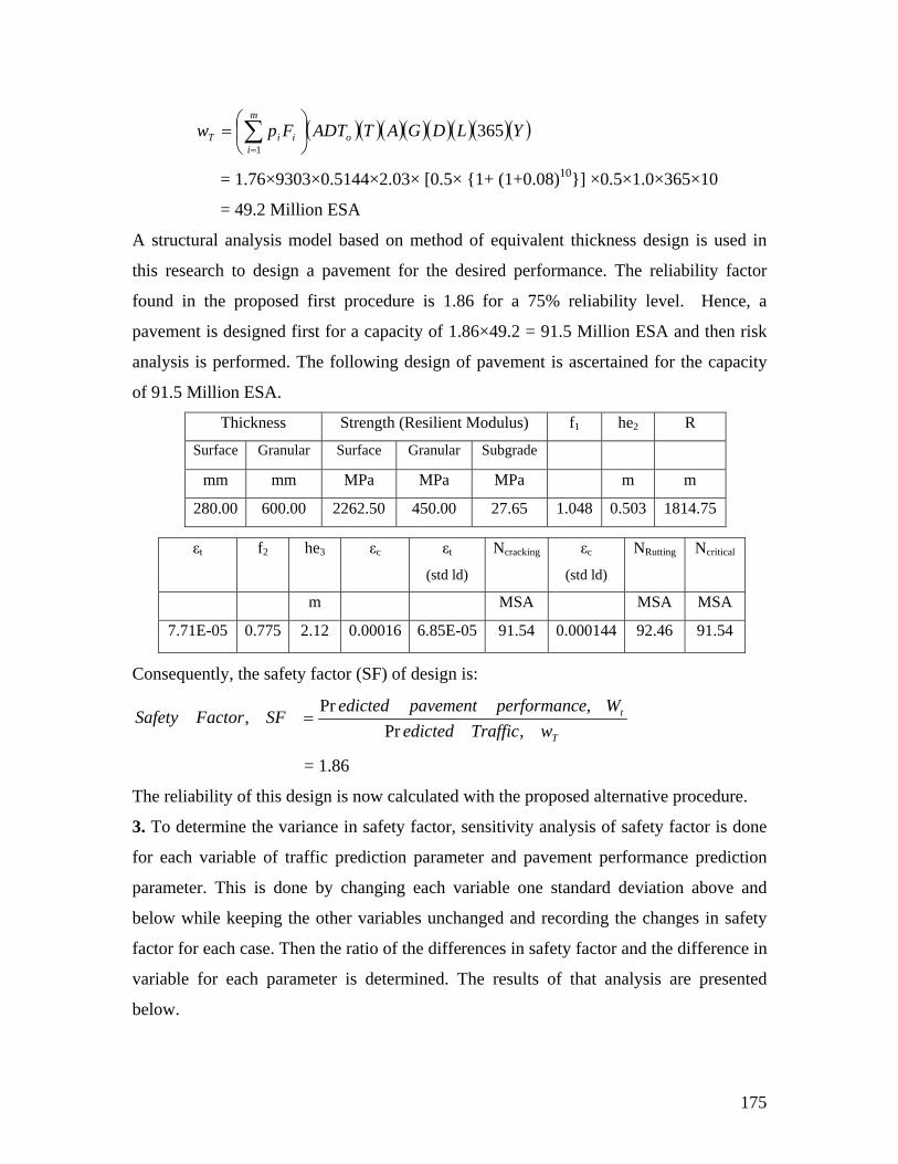
( )( )( )( )( )( )( )( )YLDGATADTFpw o
m
iiiT 365
1⎟⎠
⎞⎜⎝
⎛= ∑
=
= 1.76×9303×0.5144×2.03× [0.5× {1+ (1+0.08)10}] ×0.5×1.0×365×10
= 49.2 Million ESA
A structural analysis model based on method of equivalent thickness design is used in
this research to design a pavement for the desired performance. The reliability factor
procedure is 1.86 for a 75% reliability level. Hence, a
avement is ascertained for the capacity
o ESA.
Thickness 1
found in the proposed first
pavement is designed first for a capacity of 1.86×49.2 = 91.5 Million ESA and then risk
analysis is performed. The following design of p
f 91.5 Million
Strength (Resilient Modulus) f he2 R
Surface Su Granular Surface Granular bgrade
mm mm MPa MPa MPa m m
280.00 600. .50 450. 1.04 181400 2262 00 27.65 8 0.503 .75
he ε ε N ε )
N in N ica ε ft 2 3 c t
(std ld) cracking c
(std ld
Rutt g crit l
m A MSA MSA MS
7.71E-05 0.775 2.12 0.00016 6.85E-05 91.54 0.000144 92.46 91.54
Consequently, the safety factor (SF) of design is:
T
t
wTrafficedictedSFFactorSafety
,Pr, =
Weperformanc ,
= 1.86
The reliability of this design is now calculated with the proposed alternative procedure.
raffic prediction parameter and pavement performance prediction
parameter. This is done by changing each variable one standard deviation above and
iables unchanged and recording the changes in safety
e results of that analysis are presented
below.
pavementedictedPr
3. To determine the variance in safety factor, sensitivity analysis of safety factor is done
for each variable of t
below while keeping the other var
factor for each case. Then the ratio of the differences in safety factor and the difference in
variable for each parameter is determined. Th
175
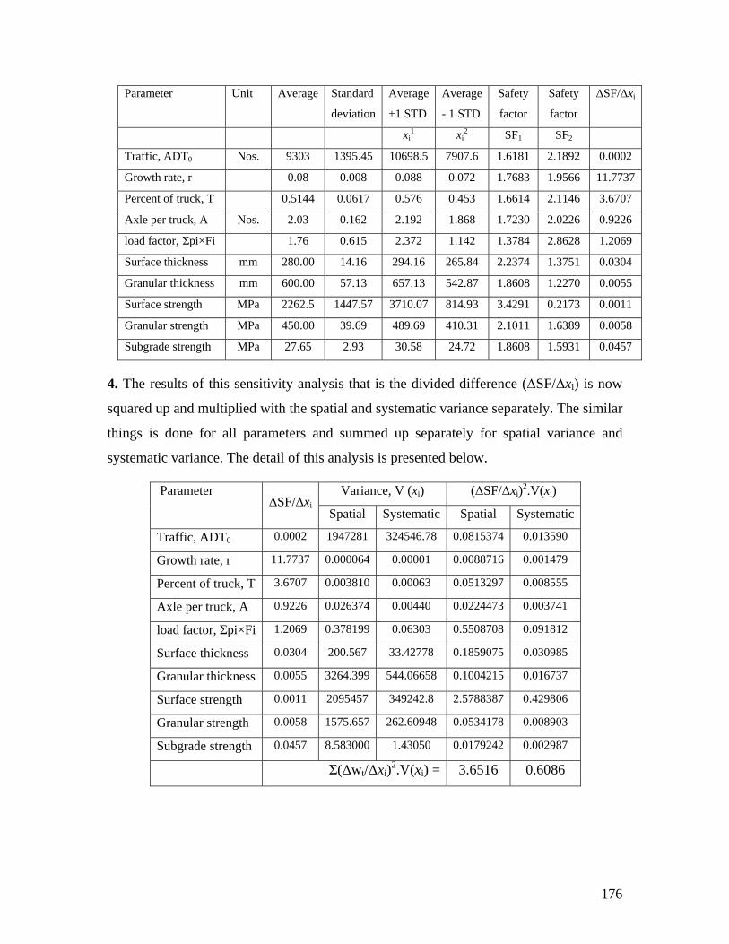
ter Unit Average Standard
deviation
Average
+1 STD
Average
- 1 STD
Safety
factor
Safety
factor
ΔSF/Δxi
Parame
xi xi SF1 SF2 1 2
Traffic, ADT Nos. 9303 1395.45 10698.5 7907.6 1.6181 2.1892 0 0.0002
Growth rate, r 0.08 0.008 0.088 0.072 1.7683 1.9566 11.7737
Percent of truck, T 0.5144 0.0617 0.576 0.453 1.6614 2.1146 3.6707
Axle per truck, A Nos. 2.03 0.162 2.192 1.868 1.7230 2.0226 0.9226
load factor, Σpi×Fi 1.76 0.615 2.372 1.142 1.3784 2.8628 1.2069
Surface thickness mm 280.00 14.16 294.16 265.84 2.2374 1.3751 0.0304
Granular thickness mm 600.00 57.13 657.13 542.87 1.8608 1.2270 0.0055
Surface strength MPa 2262.5 1447.57 3710.07 814.93 3.4291 0.2173 0.0011
Granular strength MPa 450.00 39.69 489.69 410.31 2.1011 1.6389 0.0058
Subgrade st Pa 24 1 8 1. 1 0.0457 rength M 27.65 2.93 30.58 .72 .860 593
4. The re of th nsitiv alysi is th ded difference (ΔSF/ i) is now
squared w at st va e imilar
hings is one fo all p ameters and summ
systematic variance. The detail of this analys
Variance, V ( SF/Δx )
sults is se ity an s that e divi Δx
up and multiplied ith the sp ial and sy ematic riance separat ly. The s
t d r ar ed up separately for spatial variance and
is is presented below.
(xi) Δ i)2.V(xi ParameteSF/
Spatial Sys at
r Δ Δxi
tematic Spatial System ic
Traffic, ADT0 0.0002 1947281 324546.78 0.0815374 0.013590
Growth rate, r 11.7737 0.000064 0.00001 0.0088716 0.001479
Percent of truck, T 3.6707 0.003810 0.00063 0.0513297 0.008555
Axle per truck, A 0.9226 0.026374 0.00440 0.0224473 0.003741
load factor, Σpi×Fi 1.2069 0.378199 0.06303 0.5508708 0.091812
Surface thickness 0.0304 200.567 33.42778 0.1859075 0.030985
Granular thickness 0.0055 3264.399 544.06658 0.1004215 0.016737
Surface strength 0.0011 2095457 349242.8 2.5788387 0.429806
Granular strength 0.0058 1575.657 262.60948 0.0534178 0.008903
Subgrade strength 0.0457 8.583000 1.43050 0.0179242 0.002987
Σ(Δwt/Δxi)2.V(xi) = 3.6516 0.6086
176

5. ce in saf ct c l w
The varian ety fa or (V [SF]) is now alculated in the fo lowing ay:
[ ] [ ] [xV ]systeiatiali
n
xSFxV
xSFSFV
2
1∑∑ ⎟⎟Δ
+⎟⎟⎞
⎜⎜⎝
⎛ΔΔ
=
= .6516 608
= .260
So, the variance in safety factor V [SF] = 4.2602
De liab lity in and n re ity
matic n ⎛
i i1= ⎝sp
i=
i ⎠
2⎞
⎠⎜⎜Δ
3 + 0. 6
4 2
termination of re i dex desig liabil
From
Me r, E 1
Va fact [S 260
Sta of fa [SF V [ √4. =
the above calculation, the following is found:
an safety facto [SF] = .86
riance in safety or, V F] = 4. 2
ndard deviation safety ctor, σ ] = √ SF] = 2602 2.064
Now, the reliability index (β) is calculated using the equation 5.7 as follows:
[ ][ ]SF
SFEσ
β 0.1−=
= 064.2
0.186.1 −
= 0.4
Design Reliability
17
The des is dete f a c he value
of reliab
In this c f is 66
ign reliability rmined rom stand rd normal urve area tables for t
ility index.
ase, the reliability o design found = .2%
177
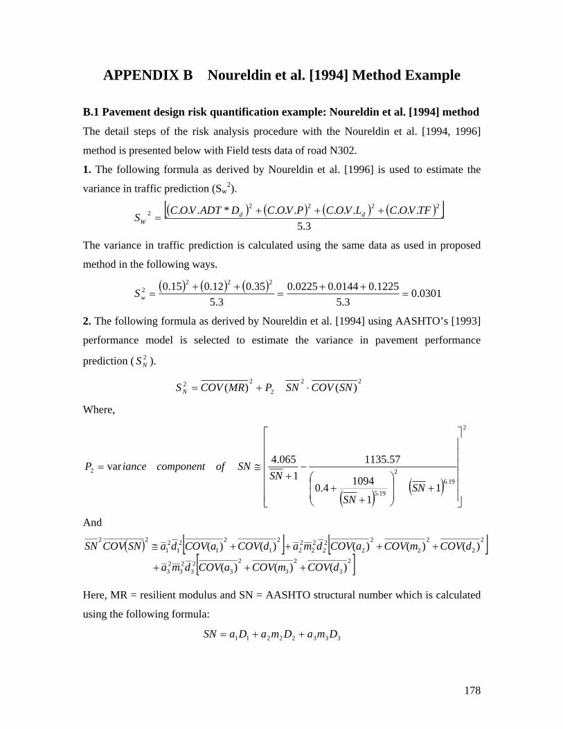
APPENDIX B Noureldin et al. [1994] Method Example
example: Noureldin et al. [1994] method
edure with the Noureldin et al. [1994, 1996]
ield tests data of road N302.
in et al. [1996] is used to estimate the
B.1 Pavement design risk quantification
The detail steps of the risk analysis proc
method is presented below with F
1. The following formula as derived by Noureld
variance in traffic prediction (Sw2).
( ) ( )[ ( ) ( ) ]
3.5.........*... 22
2 PVOCDADTVOCS d ++
=22 TFVOCLVOC d +
ated using the same data as used in proposed
W
The variance in traffic prediction is calcul
method in the following ways.
( ) ( ) ( ) 03.01225.00144.00225.035.012.015.0 2222 =
++=
++=S 01
3.53.5w
ed by Noureldin et al. [1994] using AASHTO’s [1993]
performance model is selected to estimate the variance in pavement performance
prediction ( ).
2. The following formula as deriv
2NS
22
2
22 )()( SNCOVSNPMRCOVS N ⋅+=
Where,
( ) ( )
2
19.62
19.5
2
11
10944.0
57.11351
065.4⎢var
⎥⎥⎥⎥⎥⎥
⎦
⎤
⎢⎢⎢⎢
⎢
⎣
⎡
+⎟⎟
⎠
⎞
⎜⎜
⎝
⎛
++
−+
≅=
SNSN
SNSNofcomponentiance
nd
P
A
( ) [ ] [ ][ ]2
3
2
3
2
32
323
23
2
2
2
2
2
222
22
22
2
1
2
12
12
1
22
)()()(
)()()()()(
dCOVmCOVaCOVdma
dCOVmCOVaCOVdmadCOVaCOVdaSNCOVSN
+++
++++≅
Here, MR = resilient modulus and SN = AASHTO structural number which is calculated
using the following formula:
33322211 DmaDmaDaSN ++=
178
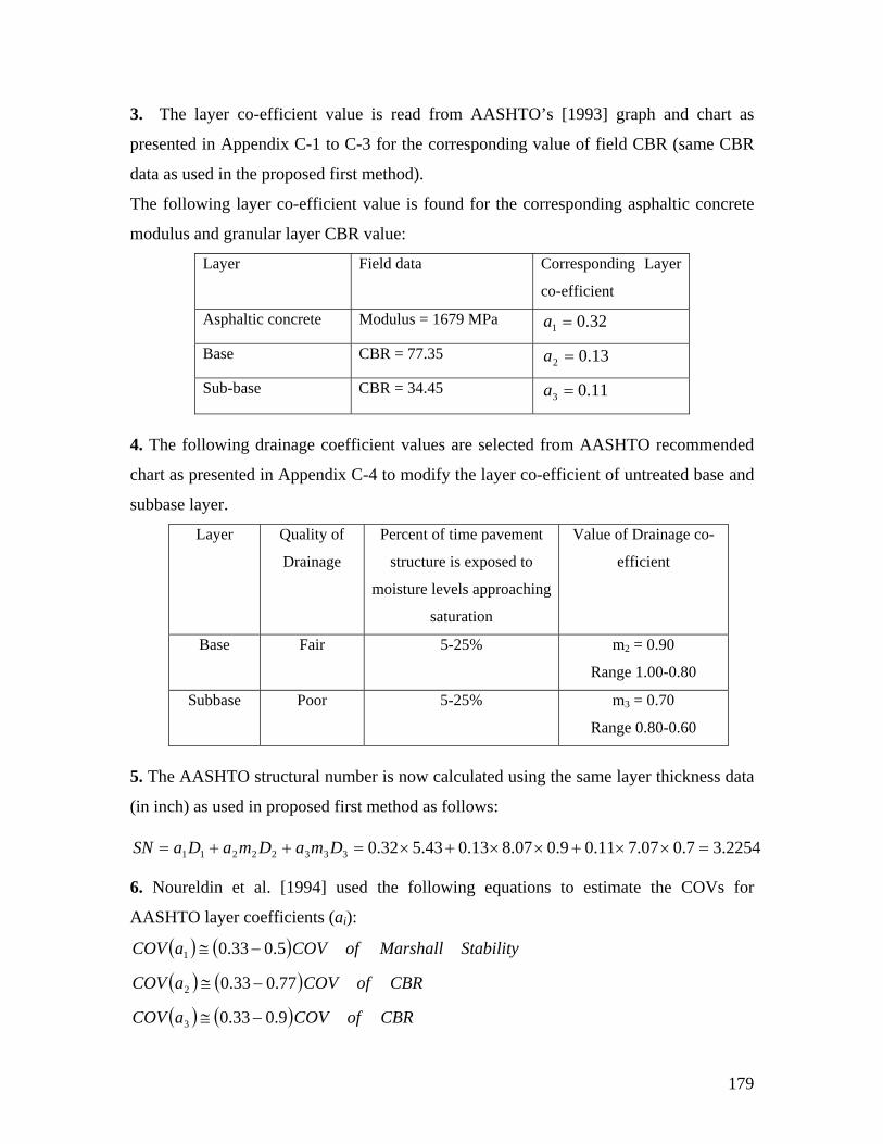
3. as
presented in Appendix C-1 to C-3 for the corresponding value of field CBR (same CBR
co-efficient
The layer co-efficient value is read from AASHTO’s [1993] graph and chart
data as used in the proposed first method).
The following layer co-efficient value is found for the corresponding asphaltic concrete
modulus and granular layer CBR value:
Layer Field data Corresponding Layer
Asphaltic concrete Modulus = 1679 MPa 32.01 =a
Base CBR = 77.35 13.02 =a
Sub-base CBR = 34.45 11.03 =a
4. The following drainage coefficient values are selected from AASHTO recommended
chart as presented in Appendix C-4 to modify the layer co-efficient of untreated base and
Drainage structure is exposed to
moisture levels approaching
saturation
efficient
subbase layer.
Layer Quality of Percent of time pavement Value of Drainage co-
Base Fair 5-25% m2 = 0.90
Range 1.00-0.80
Subbase Poor 5-25% m3 = 0.70
Range 0.80-0.60
5. The AASHTO structural number is now calculated using the same layer thickness data
ed first method as follows: (in inch) as used in propos
2254.37.007.711.09.007.813.043.532.033322211 =××+××+×=++= DmaDmaDaSN
6. Noureldin et al. [1994] used the following equations to estimate the COVs for
ASHTO layer coefficients (a ): A i
( ) ( )1 −≅ StabilityMarshallofCOVaCOV 5.033.0
( ) ( )COaCOV 77.033.02 −≅ CBRofV
( ) ( ) CBRofCOVaCOV 9.033.03 −≅
179
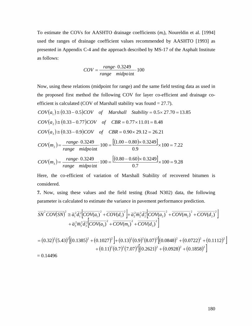
To estimate the COVs for AASHTO drainage coefficients (mi), Noureldin et al. [1994]
used the ranges of drainage coefficient values recommended by AASHTO [1993] as
presented in Appendix C-4 and the approach described by MS-17 of the Asphalt Institute
as follows:
100int
3249.0⋅
⋅=
rangeCOVmidange por
Now, using these relations (midpoint for range) and the sam
the proposed first m
efficient is lated (COV of M ity was found = 27.7).
e field testing data as used in
ethod the following COV for layer co-efficient and drainage co-
calcu arshall stabil
( ) ) 85.1370.275.05.1 ( 033.0 =×=−≅ StabilityofCOVaCOV Marshall
( ) ( ) 48.801.1177.077.033.02 =×=−≅ CBRofCOVaCOV
( ) ( ) 21.2612.2990.09.033.03 =×=−≅ CBRofCOVaCOV
( ) ( )[ ] 22.71009.0
3249.080.000.1100int
3249.0 − ×=×2 =⋅
⋅midpo
ange =rmCOV
range
( )[ ] 28.( ) 91009100int3 =×
7.0324.060.080.03249.0 ×−
=⋅
=midporange
rangemCOV
Here, the co-efficient of variation of Stability of recovered bitumen is
considere
7. Now, using these values and the field testing (Road N302) data, the following
paramet ulated to estimate the variance in pavement perform tion.
⋅
Marshall
d.
er is calc ance predic
( ) [ ] [ ][ ]22
3
2
32
323
23 )()()( dCOVmCOVaCOVdma +++
3
2
22
2
222
22
22
2
1
2
12
12
1
22)()()()()( dCOVmCOVaCOVdmadCOVaCOVdaSNCOV ++++≅
2SN
( ) ( ) ( ) ( )[ ] ( ) ( ) ( ) ( ) ( ) ( )[ ]( ) ( ) ( ) ( ) ( ) ( )[ ]222222
2222222222
1858.00928.02621.007.77.011.0
1112.00722.00848.007.89.013.01027.01385.043.532.0
+++
++++=
= 0.14496
180
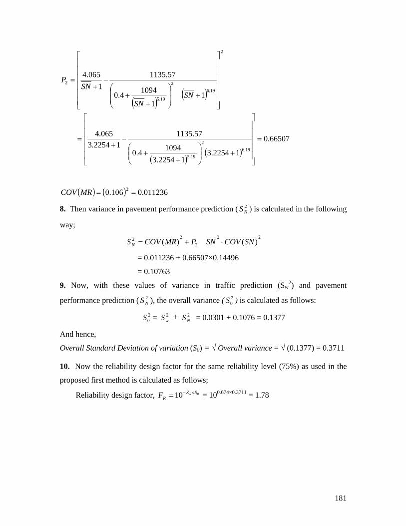
( ) ( )
( )( )
66507.0
12254.312254.3
10944.0
57.113512254.3
065.4
19.62
19.5
=
⎥⎥⎥⎥
⎦⎢⎢⎢⎢
⎣+⎟⎟
⎠
⎞⎜⎜⎝
⎛
++
−+
=
11
10944.019.6
19.5
⎥⎤
⎢
⎥⎥⎦⎢
+⎟⎟
⎠
⎞
⎜⎜
⎝
⎛
++ SN
SN
8. Then variance in pavement performance prediction ( ) is c lculated in the following
way;
57.11351
065.4
2
22 ⎥⎥⎥⎥⎤
⎢⎢⎢⎢⎢⎡
−+
=SN
P
⎡⎣
( ) ( ) 011236.0106.0 2 ==MRCOV 2NS a
22
2
22 )()( SNCOVSNPMRCOVS N ⋅+=
= 0.011236 + 0.66507×0.14496
= 0.10763
prediction ), the overall variance ( is calculated as follows:
Overall Standard Deviation of variation (S0) = √ Overall variance = √ (0.1377) = 0.3711
0. Now the reliability design factor for the same reliability level (75%) as used in the
proposed first method is calculated as follows;
Reliability design factor, = 100.674×0.3711 = 1.78
9. Now, with these values of variance in traffic prediction (Sw2) and pavement
performance ( 2NS 2
0S )
20S = 2
wS + 2NS = 0.0301 + 0.1076 = 0.1377
And hence,
1
010 SZR
RF ×−=
181
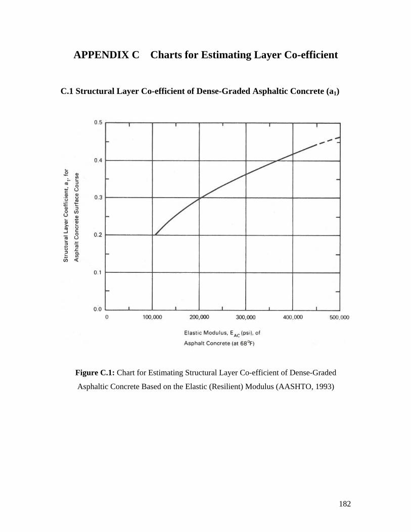
APPENDIX C Charts for Estimating Layer Co-efficient
C.1 Structural Layer Co-efficient of Dense-Graded Asphaltic Concrete (a1)
Figure C.1: Chart for Estimating Structural Layer Co-efficient of Dense-Graded
Asphaltic Concrete Based on the Elastic (Resilient) Modulus (AASHTO, 1993)
182
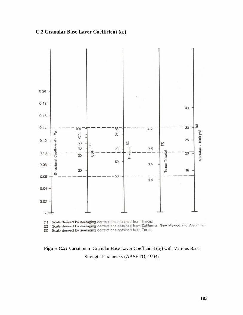
C.2
Granular Base Layer Coefficient (a2)
Figure C.2: Variation in Granular Base Layer Coefficient (a2) with Various Base
Strength Parameter AASHTO, 1993) s (
183
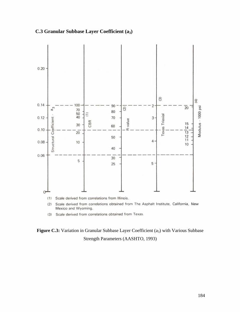
C.3 Granular Subbase Layer Coefficient (a3)
Figure C.3: Variation in Granular Subbase Layer Coefficient (a3) with Various Subbase
Strength Parameter AASHTO, 1993)
s (
184
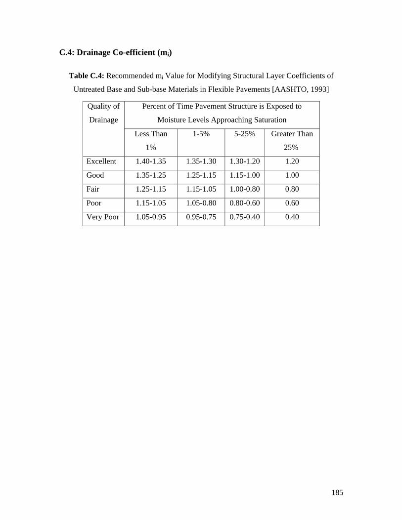
C.4: Drainage Co-efficient (mi)
Table C.4: Recommended mi Value for Modifying Structural Layer Coefficients of
Untreated Base and Sub-base Materials in Flexible Pavements [AASHTO, 1993]
Percent of Time Pavement Structure is Exposed to
Moisture Levels Approaching Saturation
Quality of
Drainage
Less Than
1%
1-5% 5-25% Greater Than
25%
Excellent 1.40-1.35 1.35-1.30 1.30-1.20 1.20
Good 1.35-1.25 1.25-1.15 1.15-1.00 1.00
Fair 1.25-1.15 1.15-1.05 1.00-0.80 0.80
Poor 1.15-1.05 1.05-0.80 0.80-0.60 0.60
Very Poor 1.05-0.95 0.95-0.75 0.75-0.40 0.40
185

APPENDIX D Definition of Different Types of Vehicle
Vehicle Type
Definition of different types of Vehicle [RHD, 2001]
Definition
Heavy T dem trucks,
the ate
Truck hree or more axles. Includes multi-axle tan
container carriers and o r articul d vehicles.
Medium Truck l 2-axle rigid trucks over three tones payload. Includes
ltura nd
Al
agricu l tractors a trailers.
Light Truck Truc neSmall k up to 3 to s payload.
Large Bus than 36 ger ch Double
r bu lud ategor
More 40 seats on foot or lon assis.
Decke ses also inc ed in this c y.
Medi nib en 1 atsum Bus (Mi us) Betwe 6 and 39 se .
Microbus Up to 16 seats.
Utility Pick-ups, jeeps and four wheels drive vehicles, such as
Pajero’s and LandRover’s.
Car/Taxi All types of car used either for personal or taxi services.
Auto Rickshaw All three wheeled motorized vehicles. Includes Babytaxi,
Mishuks, Auto-Tempo and Auto-Vans.
Motor Cycle All two wheeled motorized vehicles.
186
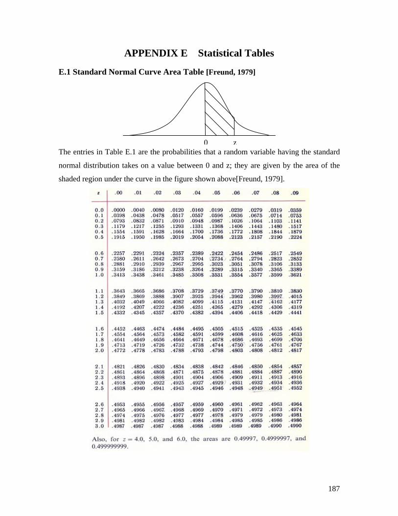
APPENDIX E Statistical Tables
E
.1 Standard Normal Curve Area Table [Freund, 1979]
The entries in Table E.1 are ariable having the standard
norm y the area of the
shaded region under the curve in
the probabilities that a random v
al distribution takes on a value between 0 and z; they are given b
the figure shown above[Freund, 1979].
0 z
187
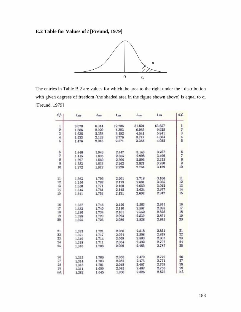
E.2 Table for Valu
es of t [Freund, 1979]
α
tα 0
The entries in Table B.2 are values for which the area to the right under the t distribution
with given degrees of freedom (the shaded area in the figure shown above) is equal to α.
[Freund, 1979]
188
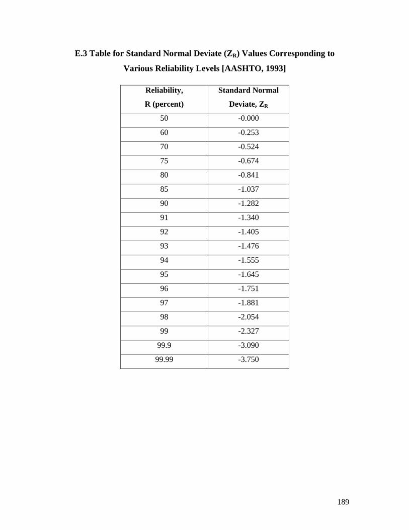
E.3 Table for Standard Normal Deviate (ZR) Values Corresponding to
Various Reliability Levels [AASHTO, 1993]
Reliability,
R (percent)
Standard Normal
Deviate, ZR
50 -0.000
60 -0.253
70 -0.524
75 -0.674
80 -0.841
85 -1.037
90 -1.282
91 -1.340
92 -1.405
93 -1.476
94 -1.555
95 -1.645
96 -1.751
97 -1.881
98 -2.054
99 -2.327
99.9 -3.090
99.99 -3.750
189

E.4
Number of Observation i
Table of Factors for Estimating Universe Standard Deviations
(After Burr, 1976)
n Subgroup C4
2 0.7979 3 0.8862 4 0.9213 5 0.9400 6 0.9515 7 0.9594 8 0.9650 9 0.9693 10 0.9727 11 0.9754 12 0.9776 13 0.9794 14 0.9810 15 0.9823 16 0.9835 17 0.9845 18 0.9854 19 0.9862 20 0.9869 21 0.9876 22 0.9882 23 0.9887 24 0.9892 25 0.9896 26 0.9901 27 0.9904 28 0.9908 29 0.9911 30 0.9914
Note: c4 is the ratio of the mean of standard deviation to universe standard deviation
190

APPENDIX F Other Tables and Graphs F.1 Strength Red g and Det ination of Design Values
uction due to Weatherin erm
Figure F.1: (a) Strength Reduction due to Weathering (b) Determination of Design Values
er Nakamura et al. 1
[Aft 998]
191
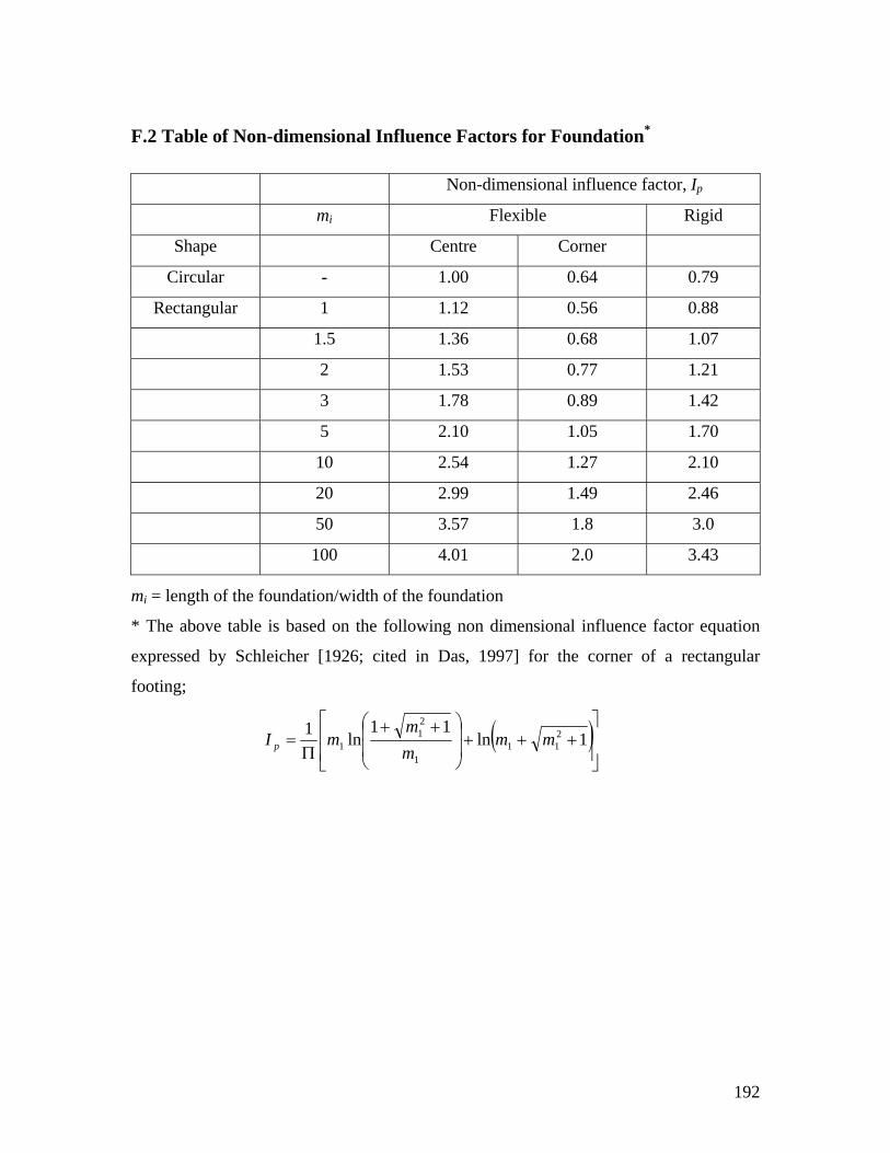
192
.2 Table of Non-dimensional Influence Factors for Foundation* F
Non-dimensional influence factor, Ip
mi Flexible Rigid
Shape Centre Corner
Circular - 1.00 0.64 0.79
Rectangular 1 1.12 0.56 0.88
1.5 1.36 0.68 1.07
2 1.53 0.77 1.21
3 1.78 0.89 1.42
5 2.10 1.05 1.70
10 2.54 1.27 2.10
20 2.99 1.49 2.46
50 3.57 1.8 3.0
100 4.01 2.0 3.43
mi = length of the foundation/width of the foundation
* The above table is based o al influence factor equation
xpressed by Schleicher [1926; cited in Das, 1997] for the corner of a rectangular
n the following non dimension
e
footing;
( )⎥⎥
⎦
⎤
⎢⎢
⎣
⎡+++⎟
⎟
⎠
⎞
⎜⎜
⎝
⎛ ++Π
= 1ln11
ln1 211
1
21
1 mmmm
mI p